ANOVA with more experimental designs

Xuhua Xia

xxia@uottawa.ca

http://dambe.bio.uottawa.ca

Xuhua Xia

Testing the effect of food (HF: high-fat) and LF: low-fat) and sex (M and F) on rabbit weight gain (WG)

Two-way experimental design

HF LF

Male 71.1 60.6

67.9 53.8

69.9 47.6

Female 65.7 50.8

59.4 50.5

67.7 53.9

WG Food Sex71.1 HF M60.6 LF M67.9 HF M53.8 LF M69.9 HF M47.6 LF M65.7 HF F50.8 LF F59.4 HF F50.5 LF F67.7 HF F53.9 LF F

Full model:fit <- aov(WG ~ Food*Sex)summary(fit) print(model.tables(fit,"means"),digits=3)boxplot(WG~Food)boxplot(WG~Sex)boxplot(WG~Food+Sex)

Save data to TwoWayANOVA.txt and retrieve into R to do analysis

Xuhua Xia

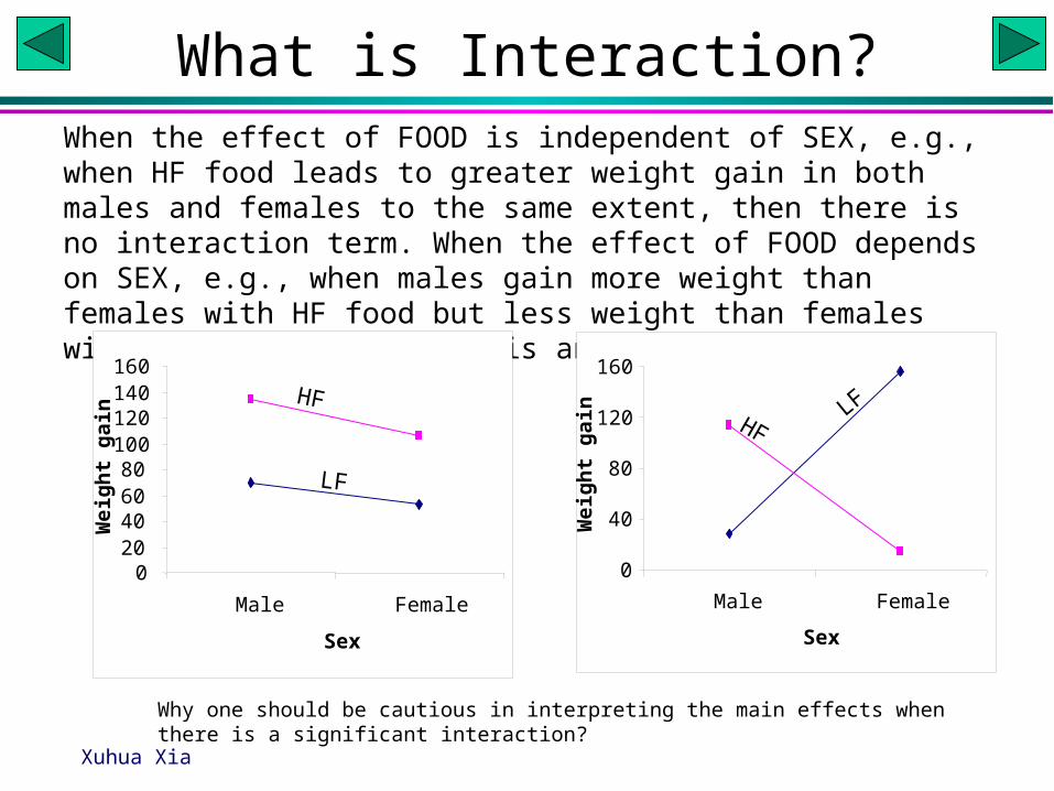
What is Interaction?When the effect of FOOD is independent of SEX, e.g., when HF food leads to greater weight gain in both males and females to the same extent, then there is no interaction term. When the effect of FOOD depends on SEX, e.g., when males gain more weight than females with HF food but less weight than females with LF food, then there is an interaction effect.

020406080

100120140160

Male Female

Sex

Wei

gh

t g

ain

0

40

80

120

160

Male Female

Sex

Wei

gh

t g

ain

HF

LF

HFLF

Why one should be cautious in interpreting the main effects when there is a significant interaction?

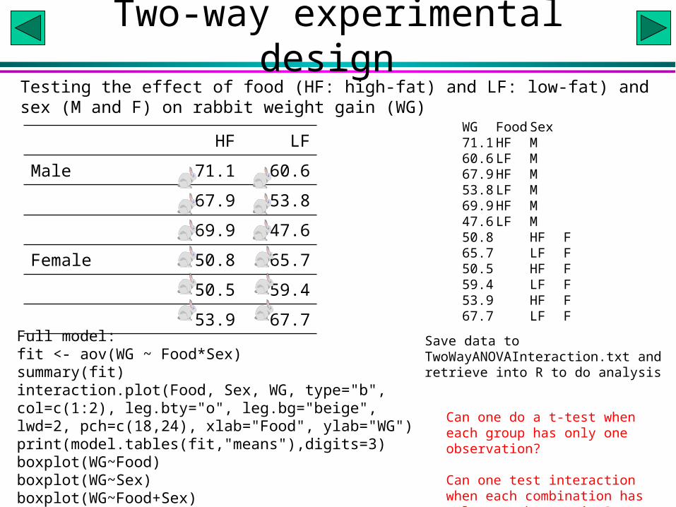
Testing the effect of food (HF: high-fat) and LF: low-fat) and sex (M and F) on rabbit weight gain (WG)

Two-way experimental design

HF LF

Male 71.1 60.6

67.9 53.8

69.9 47.6

Female 50.8 65.7

50.5 59.4

53.9 67.7

WG Food Sex71.1 HF M60.6 LF M67.9 HF M53.8 LF M69.9 HF M47.6 LF M50.8 HF F65.7 LF F50.5 HF F59.4 LF F53.9 HF F67.7 LF F

Full model:fit <- aov(WG ~ Food*Sex)summary(fit) interaction.plot(Food, Sex, WG, type="b", col=c(1:2), leg.bty="o", leg.bg="beige", lwd=2, pch=c(18,24), xlab="Food", ylab="WG")print(model.tables(fit,"means"),digits=3)boxplot(WG~Food)boxplot(WG~Sex)boxplot(WG~Food+Sex)

Save data to TwoWayANOVAInteraction.txt and retrieve into R to do analysis

Can one do a t-test when each group has only one observation?

Can one test interaction when each combination has only one observation?

Xuhua Xia

Race Sex HF LF

Short-ear Male

Female

Long-ear Male

Female

Short-ear Male 65.2, 64.5 51.1, 52.0Female 61.0, 61.2 50.0, 50.1

Long-ear Male 70.0, 71.2 60.1, 58.8Female 65.0, 65.5 55.0, 54.6

Three-way ANOVA

Organize data into four columns (WtGain, Sex, Food and Race), save to file ThreeWayANOVA.txt, retrieve into R and do data analysis.

Xuhua Xia

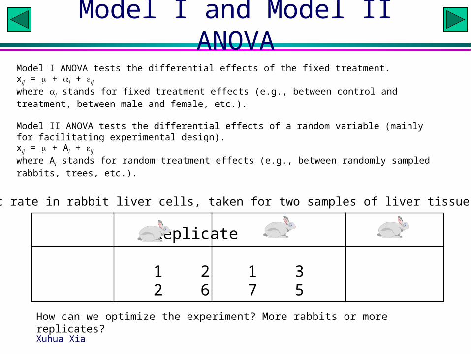
Replicate

1 2 1 32 6 7 5

Metabolic rate in rabbit liver cells, taken for two samples of liver tissue

Model I and Model II ANOVA

How can we optimize the experiment? More rabbits or more replicates?

Model I ANOVA tests the differential effects of the fixed treatment.xij = + i + ijwhere i stands for fixed treatment effects (e.g., between control and treatment, between male and female, etc.).

Model II ANOVA tests the differential effects of a random variable (mainly for facilitating experimental design).xij = + Ai + ijwhere Ai stands for random treatment effects (e.g., between randomly sampled rabbits, trees, etc.).

Xuhua Xia

Fixed and random effects• An example from a previous lecture:• Fixed effect: Difference among drugs• Random effect: Difference among subjects• Mixed ANOVA.• Using test subjects as blocks is equivalent in

design to repeated measures ANOVA or within-subject ANOVA (the last two being synonymous)

• When analyzing the data using repeated measures ANOVA, one explicitly states that one is NOT interested in the random effects. That is, one is interested only in the fixed effect, i.e., the drug effect.

• When analyzing the data using randomized complete block ANOVA, one's main interest is in the fixed effect, but one also wishes to know variations from the random effect, i.e., variation among the subjects.

• The p value for the fixed effect is the same using either repeated measures ANOVA or randomized complete block ANOVA.

Subject Drug 1 Drug 2 Drug 3

1 164 152 178

2 202 181 222

3 143 136 156

4 210 194 216

5 228 219 245

6 173 159 182

7 161 157 165

Subject Week1 Week 2 Week 3

1 Drug2 Drug1 Drug3

2 Drug1 Drug3 Drug2

3 Drug2 Drug3 Drug1

4 Drug3 Drug1 Drug2

5 Drug1 Drug2 Drug3

6 Drug3 Drug2 Drug1

7 Drug2 Drug1 Drug3

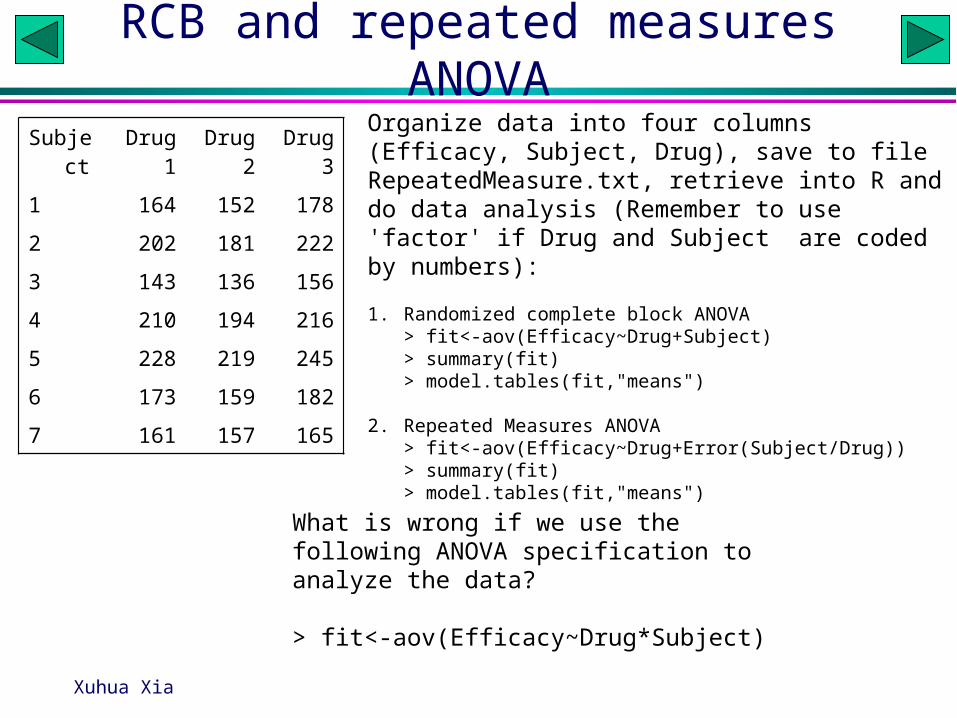
RCB and repeated measures ANOVA

Xuhua Xia

Subject Drug1 Drug2 Drug3

1 164 152 178

2 202 181 222

3 143 136 156

4 210 194 216

5 228 219 245

6 173 159 182

7 161 157 165

Organize data into four columns (Efficacy, Subject, Drug), save to file RepeatedMeasure.txt, retrieve into R and do data analysis (Remember to use 'factor' if Drug and Subject are coded by numbers):

1. Randomized complete block ANOVA> fit<-aov(Efficacy~Drug+Subject)> summary(fit)> model.tables(fit,"means")

2. Repeated Measures ANOVA> fit<-aov(Efficacy~Drug+Error(Subject/Drug))> summary(fit)> model.tables(fit,"means")

What is wrong if we use the following ANOVA specification to analyze the data?

> fit<-aov(Efficacy~Drug*Subject)

Confusing terminology in ANOVA

• Within-subject ANOVA and repeated measure ANOVA are synonymous.

• Randomized complete block design is equivalent in computation to one-way within-subject ANOVA

• When the fixed effect has only two levels, RCB, one-way within-subject ANOVA and paired-sample t-test are all equivalent and will produce the same p value given the null hypothesis of equal means.

• Ex: – Testing differences in the abundance of algal biomass between the

northern and southern sides of lakes. Fifteen lakes were used and algal biomass is measured for the northern and southern sides in each lake

– Testing differences in the expression of a gene between different organs, e.g., brain, liver, kidney. Ten female fish were used, and gene expression is measured for different tissues in each fish

Xuhua Xia

Lake Biomass at North and South Sides

Xuhua Xia

Lake North SouthL1 10 20L2 12 24L3 13 25L4 12 30L5 15 21L6 20 24L7 17 21L8 11 21L9 19 25

L10 17 30L11 14 24L12 16 29L13 19 22L14 12 29L15 10 23

Fixed effect: Difference between North and SouthRandom effect: Differences among lakes.

Null hypothesis: No difference between North and South.

Save the data to file LakeBiomass.txt and analyze the data in R.

> myDat <- read.table("LakeBiomass.txt",header=TRUE)> attach(myDat)If you use numeric value for lake, then Lake <- factor(Lake)> fit <- aov(Biomass~Site+Error(Lake/Site))> summary(fit)> model.tables(fit,"means")

In-classroom exercise:

1. Do a randomized complete block ANOVA with Lake as blocks

2. Do a paired sample t-test by either creating a data file, or by extracting data from myDat, e.g.,

> N<-subset(Biomass,Site=="North")> S<-subset(Biomass,Site=="South")> t.test(N,S,paired=T)

Compare the p value from the three significance tests.

Typical Data

> myDat <- read.table("OrganGeneExpression.txt",header=TRUE)> attach(myDat)If you use numeric value for lake, then Fish <- factor(Fish)> fit <- aov(Expr~Tissue+Error(Fish/Tissue))> summary(fit)> model.tables(fit,"means")

Fish Brain Liver Kidney

F1 33 10 50

F2 39 10 51

F3 40 10 54

F4 35 12 51

F5 38 14 51

F6 33 10 53

F7 37 12 52

F8 41 13 54

F9 37 10 55

F10 40 14 51

What are the fixed effect and random effect?

Save the data in file OrganGeneExpression.txt and analyze in R.

Twoway within-subject ANOVA

Xuhua Xia

DV: BiomassIV: Iron application (Iron): fixed effectIV: Site (North and South): fixed effectIV: Lake: random effectReorganize the data into four columns (Biomass, Lake, Iron, and Site with North and South) and save the data in file LakeIronBiomass.txt and analyze in R:

md<-read.table("LakeIronBiomass.txt",header=T)fit<-aov(Biomass~Iron*Site+Error(Lake/(Iron*Site)),md)

Lake Iron North SouthL1 Before 10 20L2 Before 12 24L3 Before 13 25L4 Before 12 30L5 Before 15 21L6 Before 20 24L7 Before 17 21L8 Before 11 21L9 Before 19 25

L10 Before 17 30L1 After 17 23L2 After 14 31L3 After 19 28L4 After 14 32L5 After 21 23L6 After 24 25L7 After 22 28L8 After 17 26L9 After 25 26

L10 After 23 37

Interpretation of results:

1. Check if there is significant interaction between Iron and Site. 2. If yes, interpret the effect of Iron at each level of Site (or the effect of Site at each

level of iron)3. If no, then interpret significant main effects (Iron and Site).

Xuhua Xia

Bartlett’s TestCtrl Treat1 Treat2 Treat3

60.8 68.7 102.6 87.957 67.7 102.1 84.265 74 100.2 83.1

58.6 66.3 96.5 85.761.7 69.8 90.3

k 4 <==Number of groups SUMn 5 5 4 5 19SS 37.568 34.26 22.97 33.552 128.35v 4 4 3 4 15Inversev 0.25 0.25 0.333333 0.25 1.083333Var 9.392 8.565 7.656667 8.388lnVar 2.239858 2.147684 2.035577 2.126802v*lnVar 8.959433 8.590737 6.10673 8.507208 32.16411PooledVar 8.556667lnPooledVar 2.146711B 0.036552 <==More accurate than that in Zar (1996)C 1.112963Bc 0.032842P 0.998433

The null hypothesis for the F-test (or variance ratio test):

H0: v1 = v2.

The null hypothesis for Bartlett’s or Levene test:

H0: v1 = v2 = ... = vn.

Save the data to a file, say, BartlettTest.txt, using "." for the missing value under Treat2.

Read the data into R by using md<-read.table(…,na.strings=".")

>bartlett.test(md)

"Bc" in the table is "K-squared" in the output of bartlett.test.

You may also organize the data into two columns, i.e., DV and IV, and then use

>bartlett.test(DV~IV)

Xuhua Xia

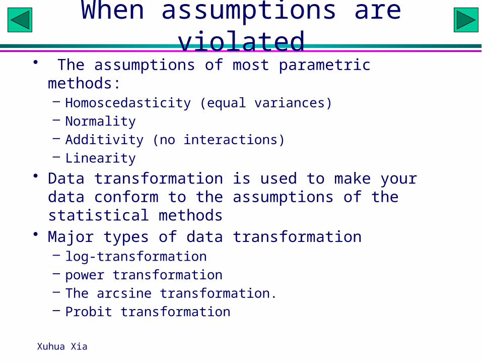
When assumptions are violated• The assumptions of most parametric methods:

– Homoscedasticity (equal variances)– Normality– Additivity (no interactions)– Linearity

• Data transformation is used to make your data conform to the assumptions of the statistical methods

• Major types of data transformation– log-transformation– power transformation– The arcsine transformation.– Probit transformation

Xuhua Xia

HomoscedasticityID Group 1 Group 21 2.72 20.092 7.39 54.603 7.39 54.604 20.09 148.415 20.09 148.416 20.09 148.417 54.60 403.438 54.60 403.439 148.41 1096.63

n 9 9Mean 37.26 275.33Var 2102.35 114784.50t -2.09df 16P 0.0530Equal Var.? P= 0.0000Kurtosis 4.89 4.89Skewness 2.12 2.12P(Zg1) 0.0046 0.0046P(Zg2) 0.0144 0.0144

• The two groups of data seem to differ greatly in means, but a t-test shows that the means do not differ significantly from each other - a surprising result.

• The two groups of data differ greatly in variance, and both deviate significantly from normality. These results invalidate the t-test.

• We calculate two ratios: var/mean ratio and Std/mean ratio (i.e., coefficient of variation).

• Group1 Group2Var/mean 56.420 416.891C.V. 1.230 1.230

• Log-transformation

Xuhua Xia

Log-Transformed DataID Group 1 Group 21 2.72 20.092 7.39 54.603 7.39 54.604 20.09 148.415 20.09 148.416 20.09 148.417 54.60 403.438 54.60 403.439 148.41 1096.63

NewX = ln(X+c), where c is a small constant, e.g., min(X)/2 or just 1 if Xmin > 2. c = 1 is used in the transformation to the left.

1.312.13

ID Group 1 Group 21 1.31 3.052 2.13 4.023 2.13 4.024 3.05 5.015 3.05 5.016 3.05 5.017 4.02 6.008 4.02 6.009 5.01 7.00

n 9 9Mean 3.08 5.01Var 1.30 1.47t -3.48df 16P 0.0031Equal Var.? P= 0.8687Kurtosis -0.35 -0.30Skewness 0.16 0.02P(Zg1) 0.82 0.97P(Zg2) 0.659393 0.684475

Indication of a successful transformation:• The variances become similar • Deviation from normality is reduced• The t-test or ANOVA reveals a highly

significant difference in means between the two groups

Xuhua Xia

ID Group 1 Group 21 1.31 3.052 2.13 4.023 2.13 4.024 3.05 5.015 3.05 5.016 3.05 5.017 4.02 6.008 4.02 6.009 5.01 7.00

n 9 9Mean 3.08 5.01Var 1.30 1.47t -3.48df 16P 0.0031Equal Var.? P= 0.8687Kurtosis -0.35 -0.30Skewness 0.16 0.02P(Zg1) 0.82 0.97P(Zg2) 0.659393 0.684475

Log-Transformed DataNewX = ln(X+1)

1 NewXeX

Transform back:

Compare this mean with the original mean. Which one is more preferable?

Calculate the standard error, the degree of freedom, and 95% CL (t0.05, 8 = 2.306).

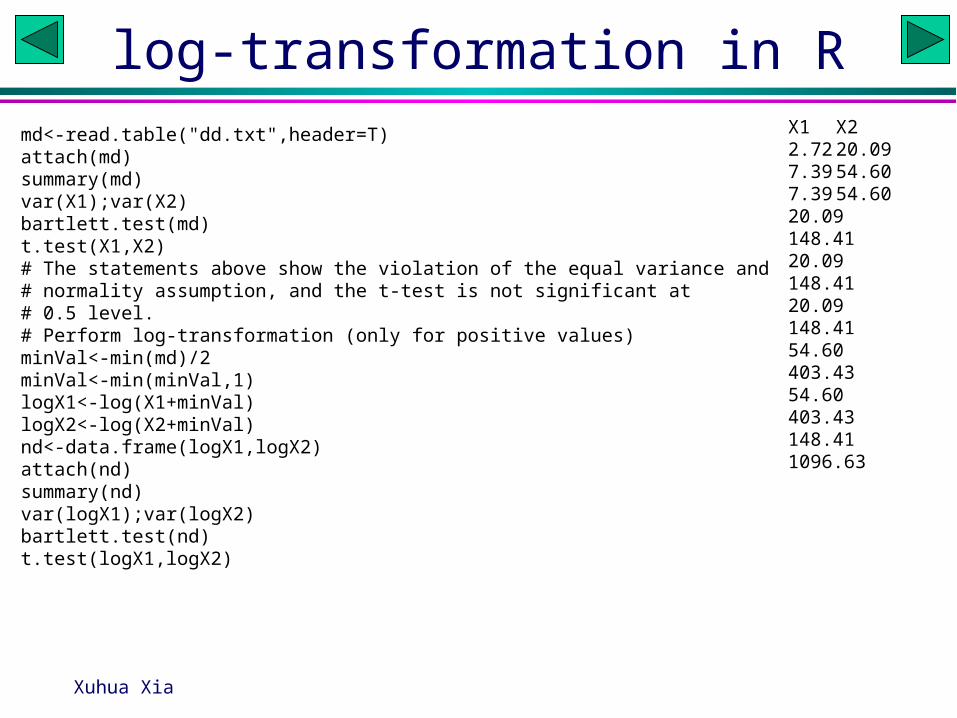
log-transformation in R

Xuhua Xia

X1 X22.72 20.097.39 54.607.39 54.6020.09 148.4120.09 148.4120.09 148.4154.60 403.4354.60 403.43148.41 1096.63

md<-read.table("dd.txt",header=T)attach(md)summary(md)var(X1);var(X2)bartlett.test(md)t.test(X1,X2)# The statements above show the violation of the equal variance and# normality assumption, and the t-test is not significant at # 0.5 level.# Perform log-transformation (only for positive values)minVal<-min(md)/2minVal<-min(minVal,1)logX1<-log(X1+minVal)logX2<-log(X2+minVal)nd<-data.frame(logX1,logX2)attach(nd)summary(nd)var(logX1);var(logX2)bartlett.test(nd)t.test(logX1,logX2)

Xuhua Xia

AdditivityFactor B Level 1 Level 2

1.313 2.4502.127 3.2402.127 3.3433.049 3.9763.049 3.5783.049 4.5074.018 4.6664.018 5.3245.007 6.060

Mean 3.084 4.1272.030 2.9272.805 3.5992.751 3.8373.968 4.9333.766 4.5763.589 4.7814.570 5.7194.562 5.9835.956 6.868

Mean 3.778 4.803

Level 1

Level 2

Factor A

• What experimental design is this?

• Compare the group means. Is there an interaction effect?

Additivity means that the difference between levels of one factor is consistent for different levels of another factor.

Xuhua Xia

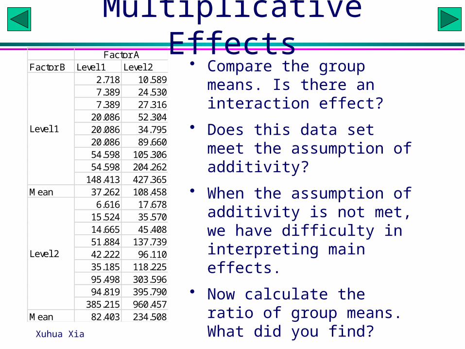
Multiplicative EffectsFactor B Level 1 Level 2

2.718 10.5897.389 24.5307.389 27.316

20.086 52.30420.086 34.79520.086 89.66054.598 105.30654.598 204.262

148.413 427.365Mean 37.262 108.458

6.616 17.67815.524 35.57014.665 45.40851.884 137.73942.222 96.11035.185 118.22595.498 303.59694.819 395.790

385.215 960.457Mean 82.403 234.508

Level 1

Level 2

Factor A• Compare the group means. Is

there an interaction effect?

• Does this data set meet the assumption of additivity?

• When the assumption of additivity is not met, we have difficulty in interpreting main effects.

• Now calculate the ratio of group means. What did you find?

Xuhua Xia

Factor B Level 1 Level 22.718 10.5897.389 24.5307.389 27.316

20.086 52.30420.086 34.79520.086 89.66054.598 105.30654.598 204.262

148.413 427.365Mean 37.262 108.458

6.616 17.67815.524 35.57014.665 45.40851.884 137.73942.222 96.11035.185 118.22595.498 303.59694.819 395.790

385.215 960.457Mean 82.403 234.508

Level 1

Level 2

Factor A

Multiplicative EffectsFor Factor A, we see that Level 2 has a mean about 2.88 times as large as that for Level 1. For factor B, Level 2 has a mean about 2.18 times as large as that for Level 1).

If you know the value for Level 1 of Factor A, you can obtain the value for Level 2 of Factor A by multiplying the known value by 2.88. Similarly, you can do the same for Factor B.

We say that the effect of Factors A and B are multiplicative, not additive.

If Y = cX, then ln(Y) = ln(c) + ln(X)

Xuhua Xia

Factor B Level 1 Level 22.718 10.5897.389 24.5307.389 27.316

20.086 52.30420.086 34.79520.086 89.66054.598 105.30654.598 204.262

148.413 427.365Mean 37.262 108.458

6.616 17.67815.524 35.57014.665 45.40851.884 137.73942.222 96.11035.185 118.22595.498 303.59694.819 395.790

385.215 960.457Mean 82.403 234.508

Level 1

Level 2

Factor A

1.312.13

Factor B Level 1 Level 21.313 2.4502.127 3.2402.127 3.3433.049 3.9763.049 3.5783.049 4.5074.018 4.6664.018 5.3245.007 6.060

Mean 3.084 4.1272.030 2.9272.805 3.5992.751 3.8373.968 4.9333.766 4.5763.589 4.7814.570 5.7194.562 5.9835.956 6.868

Mean 3.778 4.803

Level 1

Level 2

Factor A

Log-transformationNow log-transform the data. Compare the means. Is the assumption of additivity met now?

Original Data

37.262 108.4582102.351 17878.648

82.403 234.50812400.091 80241.944

3.084 4.1271.302 1.268

3.778 4.8031.235 1.385

Transformed data

Mean

Variance

log-transformation in R# first recode the data as "X FacA FacB" and save to # DataTransformTwoWayANOVA.txtmd<-read.table("DataTransformTwoWayANOVA.txt",header=T)attach(md)# Get variance for each combination of FacA and FacBlibrary(Hmisc)summary(X~interaction(FacA,FacB),data=md,method="response", fun=function(X) c(mean.X=mean(X),var.X=var(X)))bartlett.test(md)fit<-aov(X~FacA+FacB)anova(fit)# The statements above show the violation of the equal variance and normality# assumption, and the t-test is not significant at 0.5 level.# Perform log-transformation (only for positive values)minVal<-min(X)/2minVal<-min(minVal,1)lnX<-log(X+minVal)library(Hmisc)summary(lnX~interaction(FacA,FacB),data=md,method="response", fun=function(lnX) c(mean.X=mean(lnX),var.X=var(lnX)))fit<-aov(lnX~FacA+FacB)anova(fit)

Xuhua Xia

Square-Root TransformationID Group 1 Group 21 1 92 4 163 4 164 9 255 9 256 9 257 16 368 16 369 25 49

Mean 10.333 26.333Var 56.500 152.500Var/Mean 5.468 5.791Std/Mean 0.727 0.469

• The two groups of data differ much in variance.

• Calculate two ratios: var/mean ratio and Std/mean ratio (i.e., coefficient of variation).

• Does your calculation suggest log-transformation? When is log-transformation appropriate?

• Use square-root transformation when different groups have similar Variance/Mean ratios

Notice the means, which do not coincide with the most frequent observations

Xuhua Xia

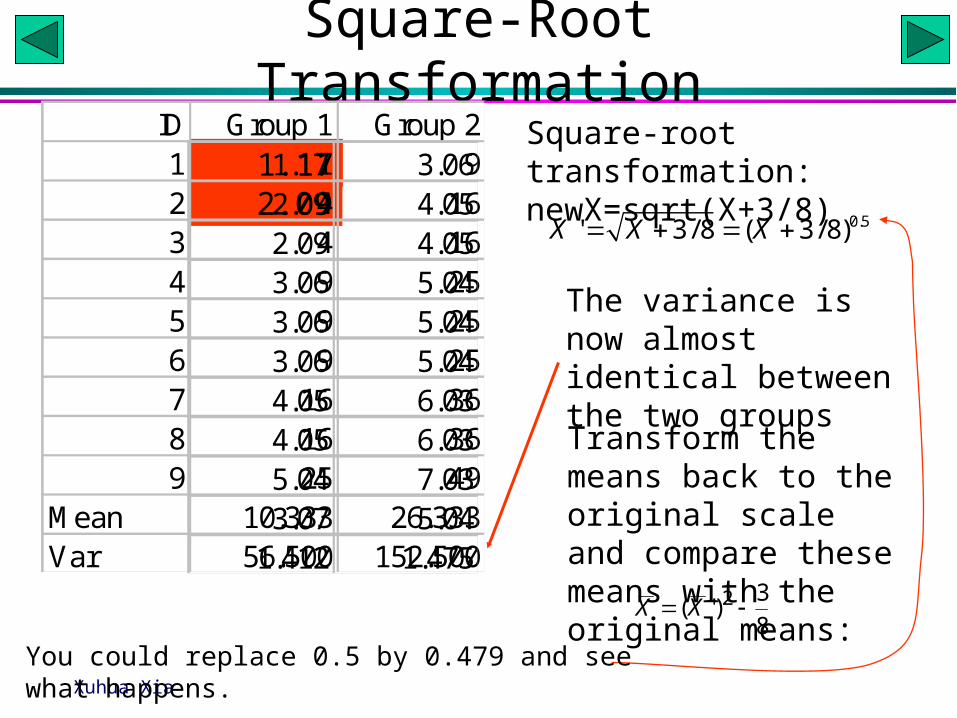
Square-Root TransformationID Group 1 Group 21 1 92 4 163 4 164 9 255 9 256 9 257 16 368 16 369 25 49

Mean 10.333 26.333Var 56.500 152.500

1.172.091.17 3.062.09 4.052.09 4.053.06 5.043.06 5.043.06 5.044.05 6.034.05 6.035.04 7.033.07 5.04

1.412 1.475

0.5' 3 / 8 ( 3 / 8)X X X

Square-root transformation:newX=sqrt(X+3/8)

The variance is now almost identical between the two groups

8

3)'( 2 XX

Transform the means back to the original scale and compare these means with the original means:

You could replace 0.5 by 0.479 and see what happens.

Xuhua Xia

Assignment: Data Transformation

1 2 3 42 6 9 20 4 5 42 8 6 13 2 5 00 4 11 2

n 5 5 5 5Mean 1.4 4.8 7.2 1.8Var 1.8 5.2 7.2 2.2SE 0.600 1.020 1.200 0.663T 2.776 2.776 2.776 2.776LowerL -0.266 1.969 3.868 -0.042UpperL 3.066 7.631 10.532 3.642

GroupThe data set is right-skewed for each group.

Calculate the variance/mean ratio and C.V. for each group, and decide what transformation you should use.

Do the transformation and convert the means back to the original scale.

Xuhua Xia

With Multiple Groups

When you have multiple groups, a “Variance vs Mean” or a “Std vs Mean” plot can help you to decide which data transformation to use. The graph on the left shows that the Var/Mean ratio is almost constant. What transformation should you use?

0

2

4

6

8

0 2 4 6 8

Mean

Var

ianc

e

Xuhua Xia

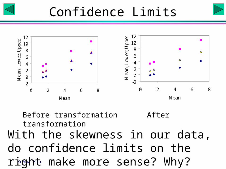
Confidence Limits

-2

0

2

4

6

8

10

12

0 2 4 6 8

Mean

Mea

n, L

ower

, Upp

er

-202468

1012

0 2 4 6 8

Mean

Mea

n, L

ower

, Upp

er

Before transformation After transformation

With the skewness in our data, do confidence limits on the right make more sense? Why?

Xuhua Xia

Arcsine Transformation

• Used for proportions• Compare the variances

before and after transformation

• Do you know how to transform the means and C.L. back to the original scale?

Group1 Group2 Group1 Group284.20 92.30 66.579 73.89088.90 95.10 70.539 77.21189.20 90.30 70.814 71.85483.40 88.60 65.957 70.26780.10 92.60 63.507 74.21581.30 96.00 64.378 78.46385.80 93.70 67.863 75.463

Mean 84.70 92.66 67.091 74.480Var 12.29 6.73 8.017 8.226SE 1.325 0.980 1.070 1.084LowerL 81.457 90.258 64.472 71.828UpperL 87.943 95.056 69.709 77.133Transform backNewMean 84.847 92.841LowerL 81.428 90.273UpperL 87.974 95.041

newX <- asin(sqrt(X))

Convert back:X <- sin(newX)^2