Embed Size (px)
Citation preview

Word Sense Disambiguation
2014.05.10
Minho Kim([email protected])
Foundation of Statistical Natural Language Processing

Motivation
• Computationally determining which sense of a word is activated by its use in a particular context.
– E.g. I am going to withdraw money from the bank.
• One of the central challenges in NLP.• Needed in:
– Machine Translation: For correct lexical choice.
– Information Retrieval: Resolving ambiguity in queries.
– Information Extraction: For accurate analysis of text.
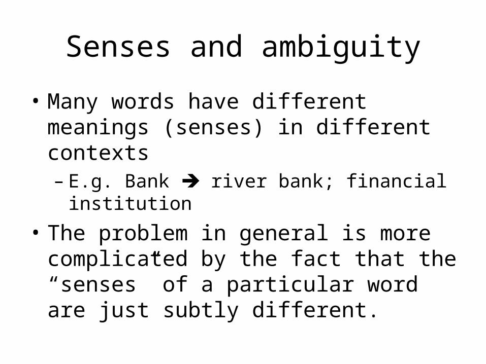
Senses and ambiguity
• Many words have different meanings (senses) in different contexts– E.g. Bank river bank; financial institution
• The problem in general is more complicated by the fact that the “senses” of a particular word are just subtly different.

Homonym and Polysemy

POS Tagging
• Some words are used in different parts of speech– “They're waiting in line at the ticket office.” Noun– “You should line a coat with fur” Verb
• The techniques used for tagging and senses disambiguation are bit different. – For tagging the local context is heavily used – looking
at the use of determiners and predicates and the like. – For word sense disambiguation the techniques look at
a broader context of the word. Tagging is explored in Chapter 10.
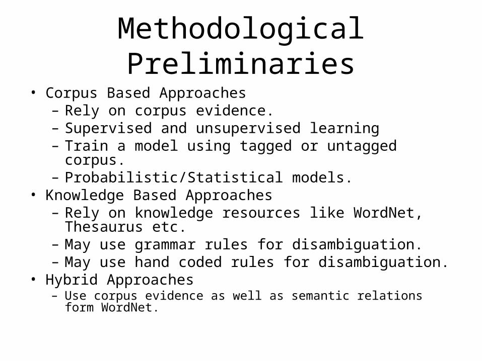
Methodological Preliminaries
• Corpus Based Approaches– Rely on corpus evidence.– Supervised and unsupervised learning– Train a model using tagged or untagged corpus.– Probabilistic/Statistical models.
• Knowledge Based Approaches– Rely on knowledge resources like WordNet,
Thesaurus etc.– May use grammar rules for disambiguation.– May use hand coded rules for disambiguation.
• Hybrid Approaches– Use corpus evidence as well as semantic relations form
WordNet.

Corpus Based Approaches
• Supervised and unsupervised learning– In supervised learning, we know the actual
“sense” of a word which is labeled – Supervised learning tends to be a classification
task– Unsupervised tends to be a clustering task
• Providing labeled corpora is expensive• Knowledge sources to help with task– Dictionaries, thesaurus, aligned bilingual texts
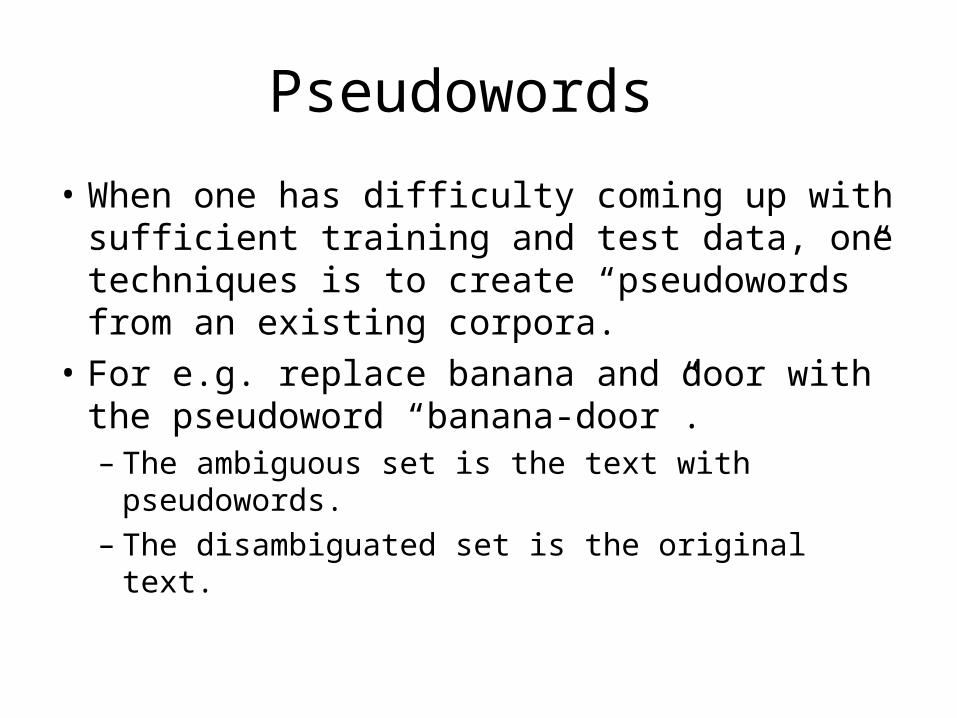
Pseudowords
• When one has difficulty coming up with sufficient training and test data, one techniques is to create “pseudowords” from an existing corpora.
• For e.g. replace banana and door with the pseudoword “banana-door”. – The ambiguous set is the text with
pseudowords. – The disambiguated set is the original text.

Upper and lower bounds
• Upper and lower bounds on performance– Upper bound is usually defined as human
performance– Lower bound is given by the simplest possible
algorithm• Most Frequent Class• Naïve Bayes
• Evaluation measure– Precision, Recall, F-measure

Supervised Disambiguation

Classification and ClusteringClass A
Class B
Class C
ModelA
B
C

Sense Tagged Corpus<p>BSAA0011-00018403 서양에만 서양 /NNG + 에 /JKB + 만 /JXBSAA0011-00018404 젤리가 젤리 /NNG + 가 /JKSBSAA0011-00018405 있는 있 /VV + 는 /ETMBSAA0011-00018406 것이 것 /NNB + 이 /JKCBSAA0011-00018407 아니라 아니 /VCN + 라 /ECBSAA0011-00018408 우리 우리 /NPBSAA0011-00018409 나라에서도 나라 /NNG + 에서 /JKB + 도 /JXBSAA0011-00018410 앵두 앵두 /NNGBSAA0011-00018411 사과 사과 __05/NNGBSAA0011-00018412 모과 모과 __02/NNGBSAA0011-00018413 살구 살구 /NNGBSAA0011-00018414 같은 같 /VA + 은 /ETMBSAA0011-00018415 과일로 과일 __01/NNG + 로 /JKBBSAA0011-00018416 '과편 '을 '/SS + 과편 /NNG + '/SS + 을 /JKOBSAA0011-00018417 만들어 만들 /VV + 어 /ECBSAA0011-00018418 먹었지만 먹 __02/VV + 었 /EP + 지만 /ECBSAA0011-00018419 수박은 수박 __01/NNG + 은 /JXBSAA0011-00018420 물기가 물기 /NNG + 가 /JKSBSAA0011-00018421 너무 너무 /MAGBSAA0011-00018422 많고 많 /VA + 고 /ECBSAA0011-00018423 펙틴질이 펙틴질 /NNG + 이 /JKSBSAA0011-00018424 없어 없 /VA + 어 /ECBSAA0011-00018425 가공해 가공 __01/NNG + 하 /XSV + 아 /ECBSAA0011-00018426 먹지 먹 __02/VV + 지 /ECBSAA0011-00018427 못했다 . 못하 /VX + 았 /EP + 다 /EF + ./SF</p>

Notational Conventions

Supervised task
• The idea here is that there is a training set of exemplars which tags each word that needs to be disambiguated with the correct “sense” of the word.
• The task is to correctly classify the word sense in the testing set using the statistical properties gleaned from the training set for the occurrence of the word in a particular context
• This chapter explores two approaches to this problem– Bayesian approach and information theoretic
approach
Bayesian Classification
16
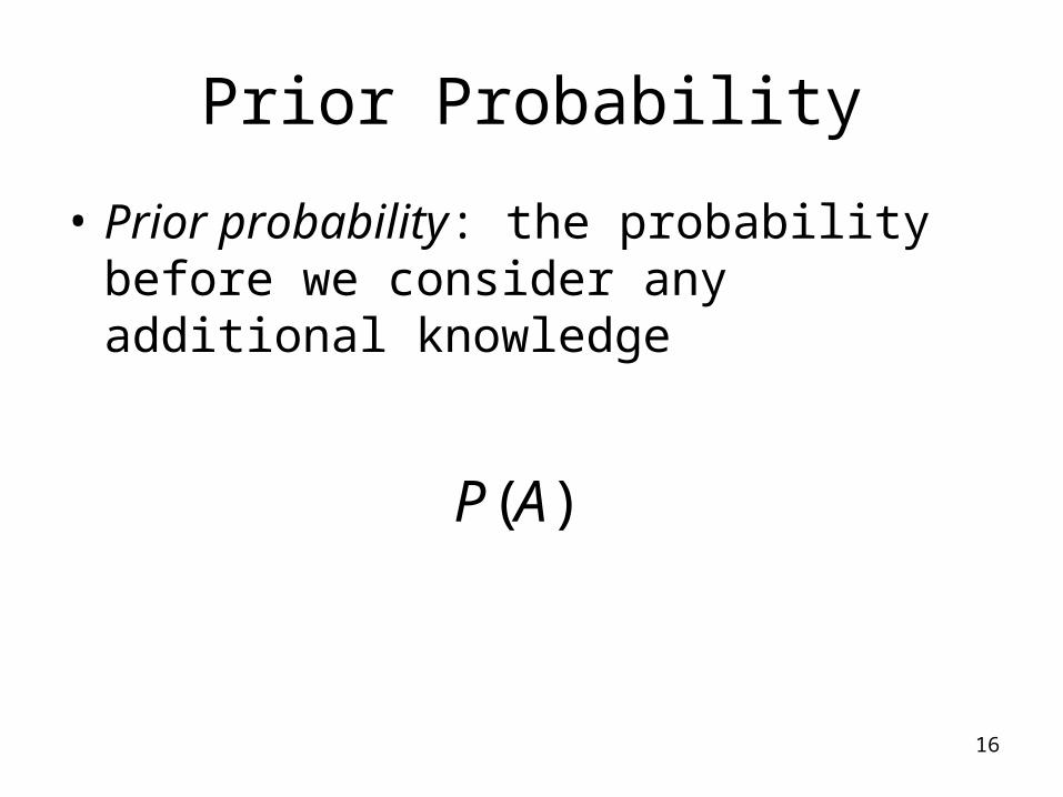
Prior Probability
• Prior probability: the probability before we consider any additional knowledge
)(AP

17
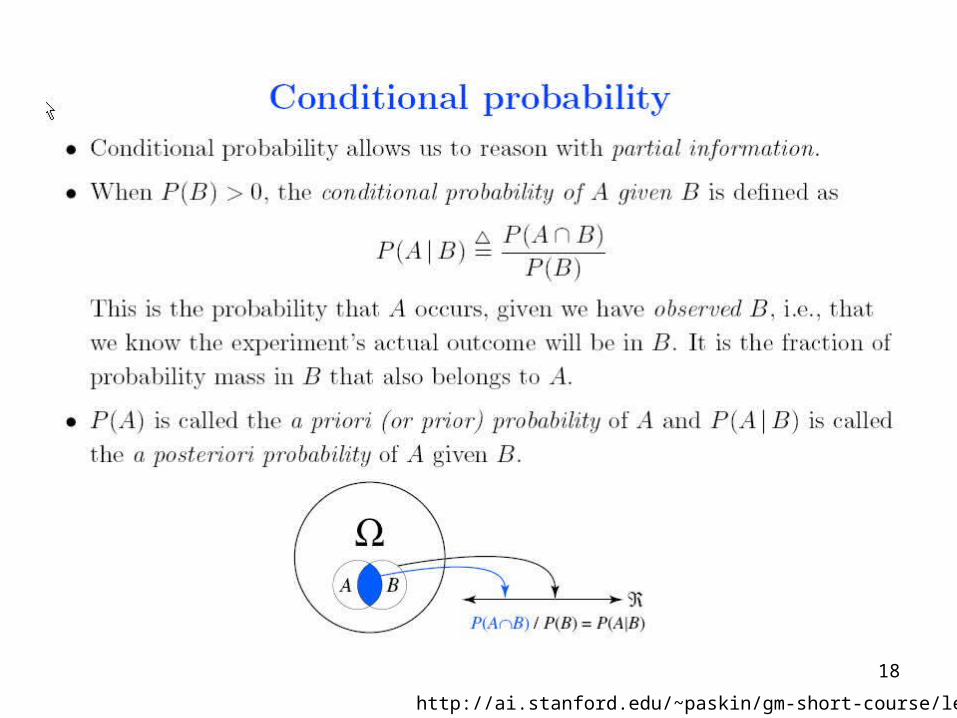
Conditional probability
• Sometimes we have partial knowledge about the outcome of an experiment
• Conditional (or Posterior) Probability
• Suppose we know that event B is true
• The probability that A is true given the knowledge about B is expressed by
)|( BAP
P(B)
P(A,B)P(A|B)
18
http://ai.stanford.edu/~paskin/gm-short-course/lec1.pdf

19
Conditional probability (cont)
)()|(
)()|(),(
APABP
BPBAPBAP
• Note: P(A,B) = P(A ∩ B) • Chain Rule• P(A, B) = P(A|B) P(B) = The probability that A and B both happen is the
probability that B happens times the probability that A happens, given B has occurred.
• P(A, B) = P(B|A) P(A) = The probability that A and B both happen is the probability that A happens times the probability that B happens, given A has occurred.
• Multi-dimensional table with a value in every cell giving the probability of that specific state occurring

20
Chain Rule
P(A,B) = P(A|B)P(B)
= P(B|A)P(A)
P(A,B,C,D…) = P(A)P(B|A)P(C|A,B)P(D|A,B,C..)

21
Chain Rule Bayes' rule
P(A,B) = P(A|B)P(B)
= P(B|A)P(A)
P(B)
P(B|A)P(A)P(A|B)
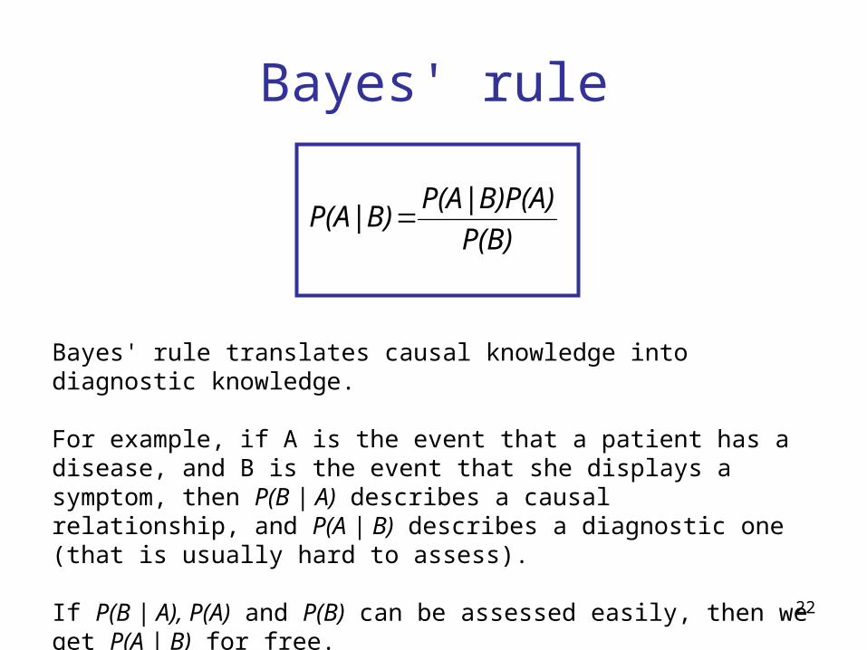
Bayes' rule
Useful when one quantity is more easy to calculate; trivial consequence of the definitions we saw but it’ s extremely useful
22
Bayes' rule
P(B)
P(A|B)P(A)P(A|B)
Bayes' rule translates causal knowledge into diagnostic knowledge.
For example, if A is the event that a patient has a disease, and B is the event that she displays a symptom, then P(B | A) describes a causal relationship, and P(A | B) describes a diagnostic one (that is usually hard to assess).
If P(B | A), P(A) and P(B) can be assessed easily, then we get P(A | B) for free.

23
Example
• S:stiff neck, M: meningitis
• P(S|M) =0.5, P(M) = 1/50,000 P(S)=1/20
• I have stiff neck, should I worry?
0002.020/1
000,50/15.0
)(
)()|()|(
SP
MPMSPSMP

24
(Conditional) independence
• Two events A e B are independent of each other if
P(A) = P(A|B)
• Two events A and B are conditionally independent of each other given C if
P(A|C) = P(A|B,C)

25
Back to language
• Statistical NLP aims to do statistical inference for the field of NLP– Topic classification
• P( topic | document ) – Language models
• P (word | previous word(s) )– WSD
• P( sense | word)
• Two main problems– Estimation: P in unknown: estimate P – Inference: We estimated P; now we want to find
(infer) the topic of a document, o the sense of a word

26
Language Models (Estimation)
• In general, for language events, P is unknown
• We need to estimate P, (or model M of the language)
• We’ll do this by looking at evidence about what P must be based on a sample of data
27
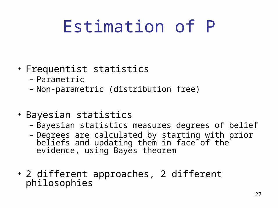
Estimation of P
• Frequentist statistics– Parametric– Non-parametric (distribution free)
• Bayesian statistics– Bayesian statistics measures degrees of belief– Degrees are calculated by starting with prior beliefs
and updating them in face of the evidence, using Bayes theorem
• 2 different approaches, 2 different philosophies

28
Inference
• The central problem of computational Probability Theory is the inference problem:
• Given a set of random variables X1, … , Xk and their joint density P(X1, … , Xk), compute one or more conditional densities given observations.– Compute
• P(X1 | X2 … , Xk)• P(X3 | X1 )• P(X1 , X2 | X3, X4,) • Etc …
• Many problems can be formulated in these terms.

29
Bayes decision rule
• w: ambiguous word• S = {s1, s2, …, sn } senses for w • C = {c1, c2, …, cn } context of w in a corpus• V = {v1, v2, …, vj } words used as contextual features for
disambiguation
• Bayes decision rule– Decide sj if P(sj | c) > P(sk | c) for sj ≠ sk
• We want to assign w to the sense s’ where
s’ = argmaxsk P(sk | c)
30
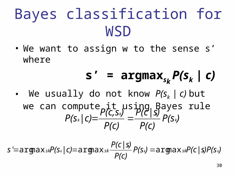
Bayes classification for WSD
• We want to assign w to the sense s’ where
s’ = argmaxsk P(sk | c)
• We usually do not know P(sk | c) but we can compute it using Bayes rule
)P(sP(c)
)P(c|s
P(c)
)P(c,s|c)P(s k
kk
k
))P(sP(c|s)P(sP(c)
)P(c|s|c)P(ss kkk
k
k sksksk maxargmaxargmaxarg'

31
Naïve Bayes classifier
))P(sP(c|ss kk
ksmaxarg'
• Naïve Bayes classifier widely used in machine learning
• Estimate P(c | sk) and P(sk)

32
Naïve Bayes classifier))P(sP(c|s
ss kk
kmaxarg'
cvj
jjj )sP(v)sc|vvP()P(c|s kkk
in
||}in {
• Estimate P(c | sk) and P(sk)• w: ambiguous word
• S = {s1, s2, …, sn } senses for w
• C = {c1, c2, …, cn } context of w in a corpus
• V = {v1, v2, …, vj } words used as contextual features for disambiguation
• Naïve Bayes assumption:

33
Naïve Bayes classifier
cvj
jjj )sP(v)sc|vvP()P(c|s kkk
in
||}in {
• Naïve Bayes assumption:
– Two consequences
– All the structure and linear ordering of words within the context is ignored bags of words model
– The presence of one word in the model is independent of the others• Not true but model “easier” and very “efficient”• “easier” “efficient” mean something specific in the probabilistic framework
– We’ll see later (but easier to estimate parameters and more efficient inference)
– Naïve Bayes assumption is inappropriate if there are strong dependencies, but often it does very well (partly because the decision may be optimal even if the assumption is not correct)

34
Naïve Bayes for WSD
)P(s)sP(vs kk
k cvj
js
in
|maxarg'
))P(sP(c|ss kk
ksmaxarg' Bayes decision rule
cvj
jjj )sP(v)sc|vvP()P(c|s kkk
in
||}in { Naïve Bayes assumption
)sC
)svC)sP(v
k
k
k
jj
(
(|
, Count of vj when sk
w)C
)sC)P(s
k
k
(
( Prior probability of sk
Estimation
35
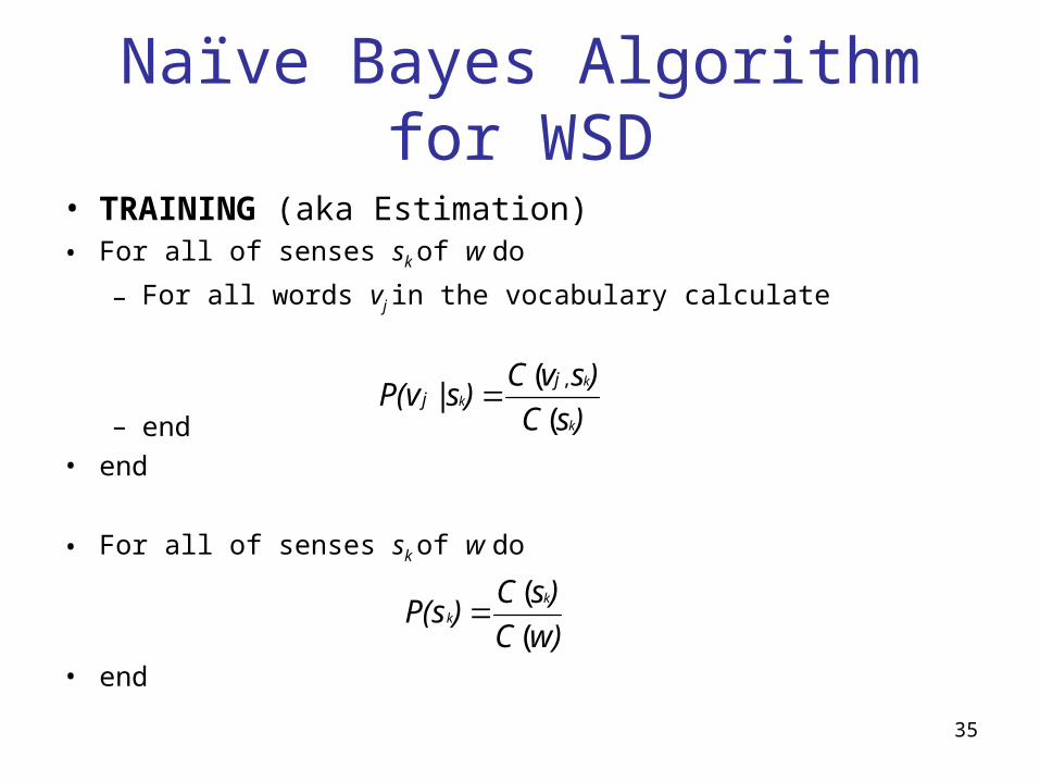
Naïve Bayes Algorithm for WSD
• TRAINING (aka Estimation)• For all of senses sk of w do
– For all words vj in the vocabulary calculate
– end• end
• For all of senses sk of w do
• end
)sC
)svC)sP(v
k
k
k
jj
(
(|
,
w)C
)sC)P(s
k
k
(
(

36
Naïve Bayes Algorithm for WSD
• TESTING (aka Inference or Disambiguation)• For all of senses sk of w do
– For all words vj in the context window c calculate
– end• end
• Choose s= sk of w do
))P(sP(c|s|c)P(s)sscore kkkk (
)sscores k
sk(maxarg'
An information-theoretic approach

Information theoretic approach
• Look for key words (informant) that disambiguates the sense of the word.

Flip-Flop Algorithm
t translations for the ambiguous wordx possible values for indicators
The algorithm works by searching for a partition of senses that maximizes the mutual information. The algorithm stops when the increase becomes insignificant.

Stepping through flip-flop algorithm for the French word: prendre

Disambiguation process
• Once the partition set for P& Q (indicator words determined), then disambiguation is simple:
1. For every occurrence of the ambiguous word, determine the value of xi – the indicator word.
2. If xi is in Q1, assign it to sense 1; if not assign it to sense 2.

Decision Lists
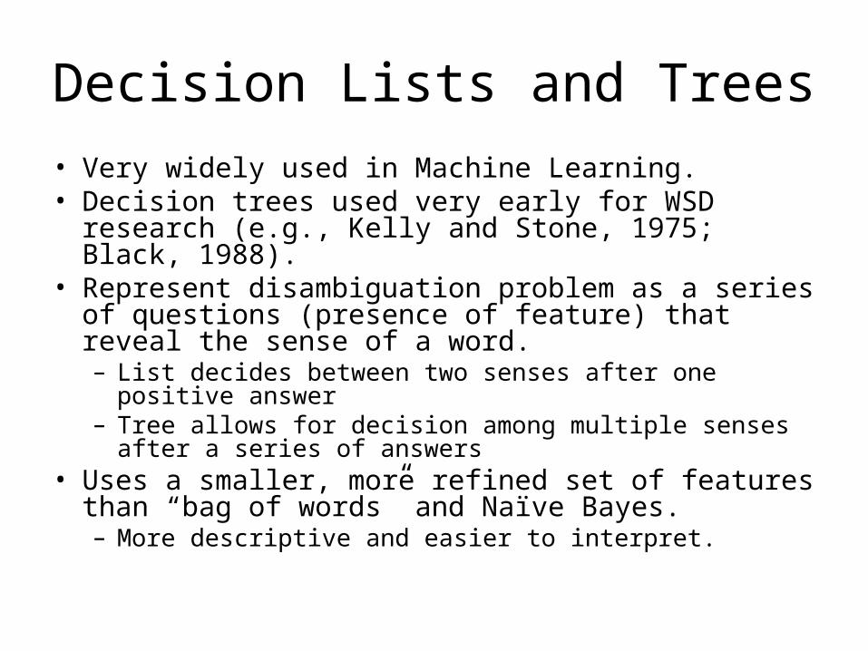
Decision Lists and Trees
• Very widely used in Machine Learning. • Decision trees used very early for WSD research (e.g.,
Kelly and Stone, 1975; Black, 1988). • Represent disambiguation problem as a series of
questions (presence of feature) that reveal the sense of a word.– List decides between two senses after one positive answer– Tree allows for decision among multiple senses after a
series of answers• Uses a smaller, more refined set of features than “bag
of words” and Naïve Bayes.– More descriptive and easier to interpret.

Decision List for WSD (Yarowsky, 1994)
• Identify collocational features from sense tagged data. • Word immediately to the left or right of target :
– I have my bank/1 statement.– The river bank/2 is muddy.
• Pair of words to immediate left or right of target :– The world’s richest bank/1 is here in New York.– The river bank/2 is muddy.
• Words found within k positions to left or right of target, where k is often 10-50 :– My credit is just horrible because my bank/1 has made
several mistakes with my account and the balance is very low.

Building the Decision List
•Sort order of collocation tests using log of conditional probabilities. •Words most indicative of one sense (and not the other) will be ranked highly.
))|2(
)|1((log
inCollocatioiFSpinCollocatioiFSp
Abs

Computing DL score– Given 2,000 instances of “bank”, 1,500 for bank/1 (financial
sense) and 500 for bank/2 (river sense)• P(S=1) = 1,500/2,000 = .75• P(S=2) = 500/2,000 = .25
– Given “credit” occurs 200 times with bank/1 and 4 times with bank/2.
• P(F1=“credit”) = 204/2,000 = .102• P(F1=“credit”|S=1) = 200/1,500 = .133• P(F1=“credit”|S=2) = 4/500 = .008
– From Bayes Rule… • P(S=1|F1=“credit”) = .133*.75/.102 = .978• P(S=2|F1=“credit”) = .008*.25/.102 = .020
– DL Score = abs (log (.978/.020)) = 3.89
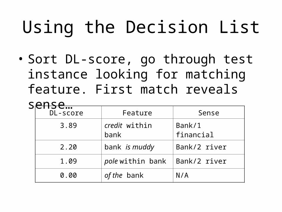
Using the Decision List
• Sort DL-score, go through test instance looking for matching feature. First match reveals sense…
DL-score Feature Sense
3.89 credit within bank Bank/1 financial
2.20 bank is muddy Bank/2 river
1.09 pole within bank Bank/2 river
0.00 of the bank N/A

Using the Decision List
CREDIT?
BANK/1 FINANCIAL IS MUDDY?
POLE? BANK/2 RIVER
BANK/2 RIVER

Support Vector Machine(SVM)

50
Linear classifiers: Which Hyperplane?
• Lots of possible solutions for a, b, c.• Some methods find a separating
hyperplane, but not the optimal one [according to some criterion of expected goodness]
– E.g., perceptron
• Support Vector Machine (SVM) finds an optimal* solution.– Maximizes the distance between the
hyperplane and the “difficult points” close to decision boundary
– One intuition: if there are no points near the decision surface, then there are no very uncertain classification decisions
This line represents the
decision boundary:
ax + by − c = 0
Ch. 15

51
Another intuition
• If you have to place a fat separator between classes, you have less choices, and so the capacity of the model has been decreased
Sec. 15.1

52
Support Vector Machine (SVM)Support vectors
Maximizesmargin
• SVMs maximize the margin around the separating hyperplane.
• A.k.a. large margin classifiers
• The decision function is fully specified by a subset of training samples, the support vectors.
• Solving SVMs is a quadratic programming problem
• Seen by many as the most successful current text classification method* *but other discriminative
methods often perform very similarly
Sec. 15.1
Narrowermargin

From Text to Feature Vectors
• My/pronoun grandfather/noun used/verb to/prep fish/verb along/adv the/det banks/SHORE of/prep the/det Mississippi/noun River/noun. (S1)
• The/det bank/FINANCE issued/verb a/det check/noun for/prep the/det amount/noun of/prep interest/noun. (S2)
P-2 P-1 P+1 P+2
fish check
river
interest
SENSE TAG
S1 adv det prep
det Y N Y N SHORE
S2 det verb
det N Y N Y FINANCE

K-NN
+
+
+
+
+
++ +
o
o
o o
o
o
oo
o
o
o
oo
o
o
o
o
o?

Supervised Approaches – Comparisons
55
Approach Average Precision
Average Recall Corpus Average Baseline Accuracy
Naïve Bayes 64.13% Not reported Senseval3 – All Words Task
60.90%
Decision Lists 96% Not applicable Tested on a set of 12 highly polysemous English words
63.9%
Exemplar Based disambiguation (k-NN)
68.6% Not reported WSJ6 containing 191 content words
63.7%
SVM 72.4% 72.4% Senseval 3 – Lexical sample task (Used for disambiguation of 57 words)
55.2%
Perceptron trained HMM
67.60 73.74% Senseval3 – All Words Task
60.90%
Dictionary-Based Discrimination

Overview
• In this section use of Dictionaries and Thesauri for the purposes of word sense disambiguation is explored.
• Lesk (1986) explores use of dictionary• Yarowsky (1992) explores use of Roget’s thesaurus.• Dagan & Itai(1994) explore the use of a bilingual
dictionary.• Also, a careful examination of the distribution properties
of words may provide additional cues. Commonly ambiguous word may not appear with more than one meaning in any given text.

Disambiguation based on sense definitions

Thesaurus-based disambiguation
• Algorithm proposed by Walker (1987)1. Comment: Given: context c
2. for all senses sk of w do
3. score(sk) = 4. end
5. choose s’ s.t. s’ = argmaxsk score(sk)
Where t(sk) is the subject code of sense sk, and
= 1; iff t(sk) is one of the subject codes of vj and 0 otherwise.
cvj jk vst )),((
)),(( jk vst

Yarowski’s adaptation
• Context is simply a 100-word window centered around the word to be disambiguated
• Algorithm adds words to the thesaurus category if it happens more often than chance in the context of that category. For instance “Navratilova” occurs more often than not only in a “sports” context if you are analyzing news articles.
• One can look at this as key markers in the context to guide the disambiguation process.

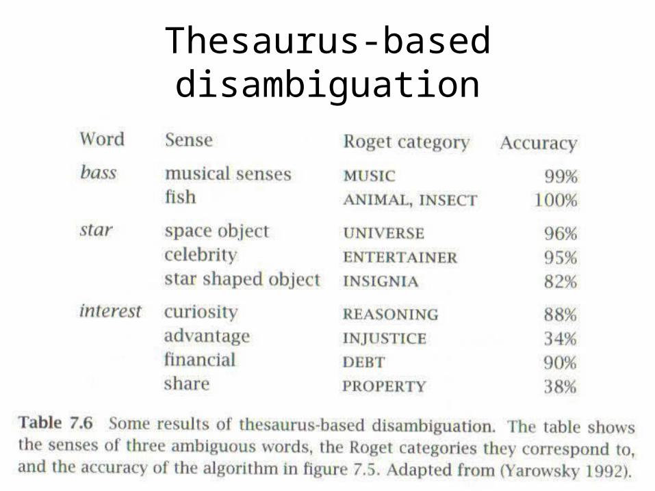
Thesaurus-based disambiguation

Disambiguation based on translations in a second-language corpus
• The insight to this methodology is that words that may have multiple senses in English tend to manifest themselves as different words in other languages. And if you have a body of translations available that you can draw upon, you can use it for disambiguation purposes.

Using Second language corpus

One sense per discourse, one sense per collocation
• One sense per discourse – the sense of a target word is highly consistent within any given document
• One sense per collocation. Nearby words provide strong and consistent clues to the sense of the word.

Example of one sense per discourse

Yarowski’s Algorithm
Unsupervised disambiguation
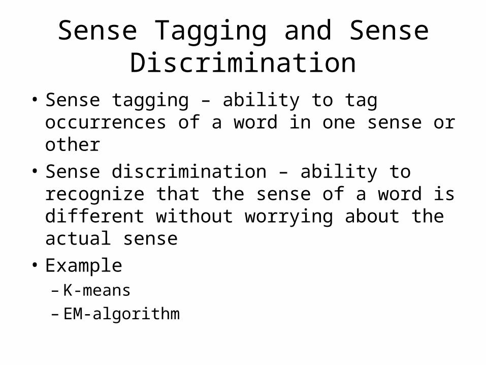
Sense Tagging and Sense Discrimination
• Sense tagging – ability to tag occurrences of a word in one sense or other
• Sense discrimination – ability to recognize that the sense of a word is different without worrying about the actual sense
• Example– K-means– EM-algorithm

70
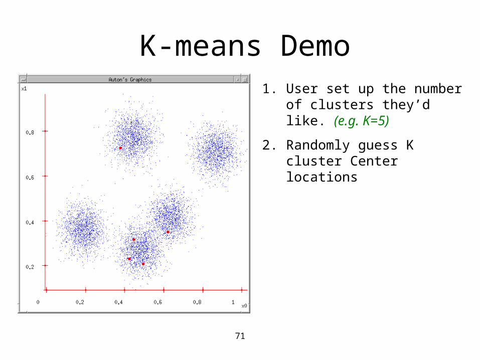
K-means Demo1. User set up the number of
clusters they’d like. (e.g. k=5)
71
K-means Demo 1. User set up the number of
clusters they’d like. (e.g. K=5)
2. Randomly guess K cluster Center locations

72
K-means Demo 1. User set up the number of
clusters they’d like. (e.g. K=5)
2. Randomly guess K cluster Center locations
3. Each data point finds out which Center it’s closest to. (Thus each Center “owns” a set of data points)
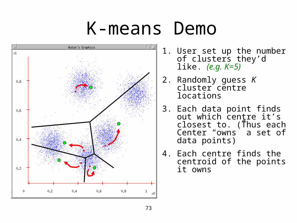
73
K-means Demo 1. User set up the number of
clusters they’d like. (e.g. K=5)
2. Randomly guess K cluster centre locations
3. Each data point finds out which centre it’s closest to. (Thus each Center “owns” a set of data points)
4. Each centre finds the centroid of the points it owns

74
K-means Demo 1. User set up the number of
clusters they’d like. (e.g. K=5)
2. Randomly guess K cluster centre locations
3. Each data point finds out which centre it’s closest to. (Thus each centre “owns” a set of data points)
4. Each centre finds the centroid of the points it owns
5. …and jumps there

75
K-means Demo 1. User set up the number of
clusters they’d like. (e.g. K=5)
2. Randomly guess K cluster centre locations
3. Each data point finds out which centre it’s closest to. (Thus each centre “owns” a set of data points)
4. Each centre finds the centroid of the points it owns
5. …and jumps there
6. …Repeat until terminated!


Disambiguation using clustering
cv
kjks
jk
svPsPs )]|(log)([logmaxarg'
Decide s’ where,
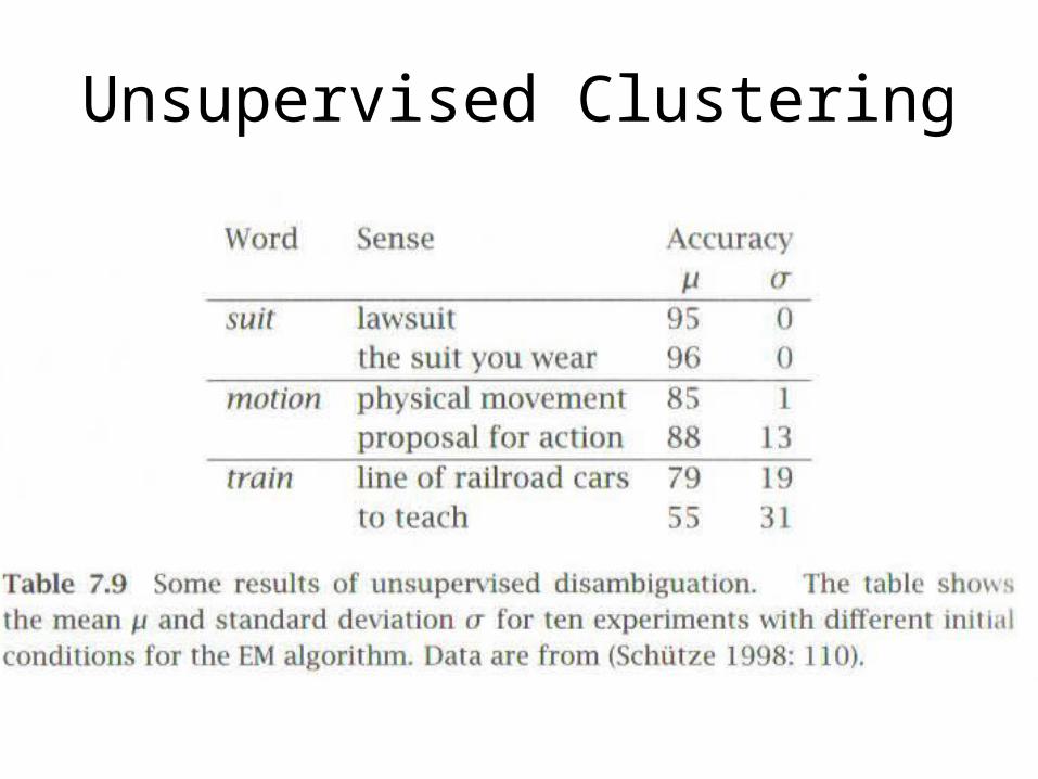
Unsupervised Clustering