Word Sense Disambiguation NPFL054/2012-2013

Introduction to Machine Learning (in NLP)

Franky

1 Project Description

A word may have more than one meaning or sense (polysemous). For instance, the word

“light” may have a meaning of “a source of lighting or illumination” as in “Turn off the light”.

It can also have a meaning of “not heavy” as in “My new phone is small and light”. The

meaning can usually be differentiated or disambiguated by observing the context where the

word is used. In a written text or sentence, the context can be described in the simplest case

as the information of the surrounding words. In a more complex case, as in the use of word

bank in “I’ll meet you at the bank”, the disambiguation requires more than just the

information from the surrounding words. Since, the bank may have a meaning of “a financial

institution (a building)” but can also have a meaning of “river bank”. Both meanings are

possible and the correct meaning will depend on the shared knowledge between the speakers.

Word sense disambiguation is the task to decide, given a text or sentence, the correct

meaning of a certain word inside the text. In this project, we experimented in disambiguating

the word senses of three different words: hard, line, and serve. We use the data developed by

(Leacock). The data contains sentences with the target word (word to be disambiguated)

tagged and disambiguated using the senses from WordNet (Fellbaum). There will be one

word that we need to disambiguate in each sentence and hence, the meaning of the word will

be disambiguated using this one sentence context.

We will use three different machine learning methods to do the classification of the word

into their respective sense. The performance of each method will be measured by its accuracy,

i.e. the number of sentences with correct prediction divided by the total number of sentences

predicted.

We will describe the data and the features we use in Section 2. Section 3 will provide

theoretical background on the selected machine learning methods. In Section 4, we will

describe our experiments and our analysis of the results. The conclusions of the work will be

given in Section 5.

2 Data and Features Description

In this section, we describe the data that we used and the features extracted from each

sentence in the data.

2.1 Development Data

The data consists of 3,833 sentences for the word “hard”, 3,646 sentences for the word “line”,

and 3,848 sentences for the word “serve”. There are 3 different senses for “hard”, 6 senses for

“line”, and 4 senses for “serve”. The sentences was further processed and enriched with

morphological (part-of-speech and lemma) and dependency information. The tokens in the

sentence are separated by space and the word to be disambiguated is enclosed in “< word >"

tag. Below is the excerpt from the data for the word “hard”:

ID: "hard-a.sjm-082_3:"

SENSE: HARD1

SENTENCE: `` it 's <hard> to explain .

MORPH: ``/`` it/PRP 's/VBZ hard/JJ to/TO explain/VB ./.

WLT: ``|``|``it|it|PRP 's|be|VBZ hard|hard|JJ to|to|TO

explain|explain|VB .|.|.

PARSE: nsubj(hard-4, it-2);cop(hard-4, 's-3);root(ROOT-0, hard-

4);aux(explain-6, to-5);xcomp(hard-4, explain-6)

Table 1 shows the description of each line in the data.

Table 1 Description of the Data

Name Description

ID Identification number of the sentence

SENSE The correct sense of the word

SENTENCE The sentence where the word is used

MORPH Morphological tag of each word (Penn Treebank Tag Set)

WLT Morphological tag with lemma of each word

PARSE Syntactic dependency of each word (Stanford Dependency Parser)

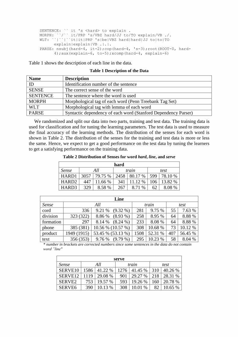
We randomized and split our data into two parts, training and test data. The training data is

used for classification and for tuning the learning parameters. The test data is used to measure

the final accuracy of the learning methods. The distribution of the senses for each word is

shown in Table 2. The distribution of the senses for the training and test data is more or less

the same. Hence, we expect to get a good performance on the test data by tuning the learners

to get a satisfying performance on the training data.

Table 2 Distribution of Senses for word hard, line, and serve

hard

Sense All train test

HARD1 3057 79.75 % 2458 80.17 % 599 78.10 %

HARD2 447 11.66 % 341 11.12 % 106 13.82 %

HARD3 329 8.58 % 267 8.71 % 62 8.08 %

Line

Sense All train test

cord 336 9.21 % (9.32 %) 281 9.75 % 55 7.63 %

division 323 (322) 8.86 % (8.93 %) 258 8.95 % 64 8.88 %

formation 297 8.14 % (8.24 %) 233 8.08 % 64 8.88 %

phone 385 (381) 10.56 % (10.57 %) 308 10.68 % 73 10.12 %

product 1949 (1915) 53.45 % (53.13 %) 1508 52.31 % 407 56.45 %

text 356 (353) 9.76 % (9.79 %) 295 10.23 % 58 8.04 % * number in brackets are corrected numbers since some sentences in the data do not contain

word ”line"

serve

Sense All train test

SERVE10 1586 41.22 % 1276 41.45 % 310 40.26 %

SERVE12 1119 29.08 % 901 29.27 % 218 28.31 %

SERVE2 753 19.57 % 593 19.26 % 160 20.78 %

SERVE6 390 10.13 % 308 10.01 % 82 10.65 %

2.2 Features Set

The features used in word sense disambiguation can be differentiated into features that use

surrounding surface words as information, such as bag of words or collocations information,

and features that use syntactic or dependency information, e.g. tense of the word, presence of

adjective at previous one position, and many others. In our work, we defined features that are

more heavily incline to the later. This is because we consider that the use of plain words will

not generalize enough for different words. Although, it might be possible that the use of

simple plain surrounding words might produce better results.

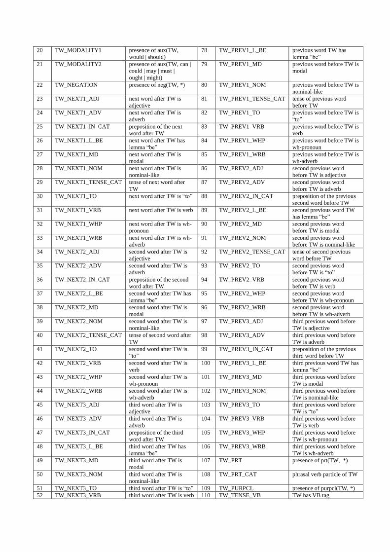
We defined 116 features that consist of binary and categorical features extracted from the

information available in the data. The features were defined based on the observation of the

sentences inside the data. In the experiment, all the features will be converted into binary

features. The complete list of features and their definitions are listed in Table 3.

As can be seen from the table, the feature such as TW_PHONE_BEFORE (63) is a feature that

depends on the information of the surface (plain) words, i.e. whether the plain word “phone”

occurs before the target word. In the other hand, the feature TW_NN_DEP_N (56) is a feature that

uses dependency information of whether the target word has a dependency nn (noun

compound modifier) with a noun word.

Table 3 Features Description

* TW: target word (word to be disambiguated)

No. Feature Name Description No. Feature Name Description

1 TW_ACOMP presence of acomp(*, TW) 59 TW_NSUBJ_DEP_N nsubject of target word is

NN|NNS

2 TW_ADVCL presence of advcl(TW, *) 60 TW_NSUBJ_DEP_P nsubject of target word is

NNP|NNPS|PRP

3 TW_ADVMOD presence of advmod(TW,

*)

61 TW_NUM presence of num(TW, *)

4 TW_AMOD presence of amod(*, TW) 62 TW_OBJECT presence of any object

5 TW_AMOD_DEP_JJ amod of target word is JJ 63 TW_PHONE_BEFORE presence of cue words

(.*phone.*|direct|subscribe.

*|toll-.*) before the TW

6 TW_APOSS_BEFORE presence of "'s" before TW 64 TW_PLURAL_OB presence of any object in

the plural form

7 TW_APOSS_DEP_N aposs of target word is

NN|NNS

65 TW_PLURAL_SB presence of any subject in

the plural form

8 TW_AUXPASS presence of auxpass(TW,

*)

66 TW_POSS_DEP_NP poss of target word is

NNP|NNPS

9 TW_CCOMP presence of ccomp(TW, *) 67 TW_POSS_DEP_P poss of target word is

PRP|PRP$

10 TW_COLON_AFTER presence of ":" after TW 68 TW_PREPC_P_CAT prepositional clausal

modifier of TW

11 TW_COMPLM presence of complm(TW,

*)

69 TW_PREP_AS_DEP_N prep_as of target word is

NN|NNS

12 TW_CONJ_AND_NN presence of and(TW, NN)

or and(NN, TW)

70 TW_PREP_BETWEEN presence of

prep_between(TW, *)

13 TW_CSUBJ presence of csubj(TW, *) 71 TW_PREP_CAT prepositional modifier of

TW

14 TW_CSUBJPASS presence of csubjpass(TW,

*)

72 TW_PREP_INCL_N prep_including of target

word is NN|NNS

15 TW_DET_CAT determiner of the target

word

73 TW_PREP_OF presence of prep_of(TW, *)

16 TW_DOBJ presence of dobj(TW, *) 74 TW_PREP_OF_DEP_N prep_of of target word is

NN|NNS

17 TW_DOBJ_OF TW is dobj 75 TW_PREV1_ADJ previous word before TW is

adjective

18 TW_IOBJ presence of iobj(TW, *) 76 TW_PREV1_ADV previous word before TW is

adverb

19 TW_MARK_CAT marker of TW 77 TW_PREV1_IN_CAT preposition of the previous

word before TW

20 TW_MODALITY1 presence of aux(TW,

would | should)

78 TW_PREV1_L_BE previous word TW has

lemma “be”

21 TW_MODALITY2 presence of aux(TW, can |

could | may | must |

ought | might)

79 TW_PREV1_MD previous word before TW is

modal

22 TW_NEGATION presence of neg(TW, *) 80 TW_PREV1_NOM previous word before TW is

nominal-like

23 TW_NEXT1_ADJ next word after TW is

adjective

81 TW_PREV1_TENSE_CAT tense of previous word

before TW

24 TW_NEXT1_ADV next word after TW is

adverb

82 TW_PREV1_TO previous word before TW is

“to”

25 TW_NEXT1_IN_CAT preposition of the next

word after TW

83 TW_PREV1_VRB previous word before TW is

verb

26 TW_NEXT1_L_BE next word after TW has

lemma “be”

84 TW_PREV1_WHP previous word before TW is

wh-pronoun

27 TW_NEXT1_MD next word after TW is

modal

85 TW_PREV1_WRB previous word before TW is

wh-adverb

28 TW_NEXT1_NOM next word after TW is

nominal-like

86 TW_PREV2_ADJ second previous word

before TW is adjective

29 TW_NEXT1_TENSE_CAT tense of next word after

TW

87 TW_PREV2_ADV second previous word

before TW is adverb

30 TW_NEXT1_TO next word after TW is “to” 88 TW_PREV2_IN_CAT preposition of the previous

second word before TW

31 TW_NEXT1_VRB next word after TW is verb 89 TW_PREV2_L_BE second previous word TW

has lemma “be”

32 TW_NEXT1_WHP next word after TW is wh-

pronoun

90 TW_PREV2_MD second previous word

before TW is modal

33 TW_NEXT1_WRB next word after TW is wh-

adverb

91 TW_PREV2_NOM second previous word

before TW is nominal-like

34 TW_NEXT2_ADJ second word after TW is

adjective

92 TW_PREV2_TENSE_CAT tense of second previous

word before TW

35 TW_NEXT2_ADV second word after TW is

adverb

93 TW_PREV2_TO second previous word

before TW is “to”

36 TW_NEXT2_IN_CAT preposition of the second

word after TW

94 TW_PREV2_VRB second previous word

before TW is verb

37 TW_NEXT2_L_BE second word after TW has

lemma “be”

95 TW_PREV2_WHP second previous word

before TW is wh-pronoun

38 TW_NEXT2_MD second word after TW is

modal

96 TW_PREV2_WRB second previous word

before TW is wh-adverb

39 TW_NEXT2_NOM second word after TW is

nominal-like

97 TW_PREV3_ADJ third previous word before

TW is adjective

40 TW_NEXT2_TENSE_CAT tense of second word after

TW

98 TW_PREV3_ADV third previous word before

TW is adverb

41 TW_NEXT2_TO second word after TW is

“to”

99 TW_PREV3_IN_CAT preposition of the previous

third word before TW

42 TW_NEXT2_VRB second word after TW is

verb

100 TW_PREV3_L_BE third previous word TW has

lemma “be”

43 TW_NEXT2_WHP second word after TW is

wh-pronoun

101 TW_PREV3_MD third previous word before

TW is modal

44 TW_NEXT2_WRB second word after TW is

wh-adverb

102 TW_PREV3_NOM third previous word before

TW is nominal-like

45 TW_NEXT3_ADJ third word after TW is

adjective

103 TW_PREV3_TO third previous word before

TW is “to”

46 TW_NEXT3_ADV third word after TW is

adverb

104 TW_PREV3_VRB third previous word before

TW is verb

47 TW_NEXT3_IN_CAT preposition of the third

word after TW

105 TW_PREV3_WHP third previous word before

TW is wh-pronoun

48 TW_NEXT3_L_BE third word after TW has

lemma “be”

106 TW_PREV3_WRB third previous word before

TW is wh-adverb

49 TW_NEXT3_MD third word after TW is

modal

107 TW_PRT presence of prt(TW, *)

50 TW_NEXT3_NOM third word after TW is

nominal-like

108 TW_PRT_CAT phrasal verb particle of TW

51 TW_NEXT3_TO third word after TW is “to” 109 TW_PURPCL presence of purpcl(TW, *)

52 TW_NEXT3_VRB third word after TW is verb 110 TW_TENSE_VB TW has VB tag

53 TW_NEXT3_WHP third word after TW is wh-

pronoun

111 TW_TENSE_VBD TW has VBD tag

54 TW_NEXT3_WRB third word after TW is wh-

adverb

112 TW_TENSE_VBG TW has VBG tag

55 TW_NN presence of nn(TW, *) 113 TW_TENSE_VBN TW has VBN tag

56 TW_NN_DEP_N nn of target word is

NN|NNS

114 TW_TENSE_VBP TW has VBP tag

57 TW_NSUBJ presence of nsubj(TW,*) 115 TW_TMOD presence of tmod(TW, *)

58 TW_NSUBJPASS presence of nsubjpass(TW,

*)

116 TW_XCOMP presence of xcomp(*,TW)

3 Machine Learning Methods

We present in this section the overview of the machine learning methods that we used in our

current work.

3.1 Selecting Machine Learning Methods

Selecting the appropriate machine learning methods might not be easy and depends on

several factors. One possibility in selecting the learners might be to try all possible learners to

get the best ones. Although, some more data-oriented criteria might also be used for the

selection, some of them are:

Linear separability of the data

Linearity of the data should be considered when selecting the learners since not all

learners can produce a non-linear boundary. A linear method might produce a high bias

for non-linear problems (Manning, chap. 14.6). However, it might not be easy to

visualize the data with high dimensions to see whether the data is linearly separable or

not.

Features dependency

A learner like Naïve Bayes use independence assumption for its features. If our defined

features are not independent, the resulting classification performance might be low. We

observed that most of our features are not independent, as in the use of _NEXT1_ADJ

and _NEXT1_TO. The occurrence of a class “adjective” in the next position after the

target word is surely to produce the non-occurrence of word “to”.

Size of the data

In we only have small amount of data, the guideline is to use the classifier with high bias,

such as Naïve Bayes. If the data is big enough, the classifier with low bias, such as k-NN,

might be used. (Manning, chap. 15.3.1)

In this work, we selected three machine learning methods to be used in our experiments.

Other than Naïve Bayes that depends on the features dependency and data size criteria, the

other machine learning methods seems to be good candidates for the task. In order to decide,

we added some additional selection criteria that are quite simple, which are based on:

The known performance (popularity) of the method: to ensure that we can get the best

results by building classifiers from learners that are known to produce good

performances in other classification tasks.

Representativeness of the learner’s class (e.g. tree-based, instance-based): to roughly

compare the different approaches.

SVM and Random Forests were selected as our first two learners because both are known

to have good performances. Since Random Forests is in its core a collection of decision trees,

we decided to omit the Decision Tree learner from the selection. The last method that we

chose was k-NN as the representative of instance-based learner. At first, we also considered

to use Naïve Bayes in our experiment. However, our preliminary experiments with Naïve

Bayes produced unsatisfying results. We think that this was probably caused by the features

that we used in this experiment which are not completely independent.

3.2 Support Vector Machine (SVM)

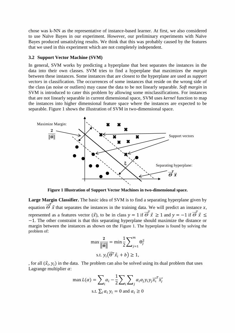
In general, SVM works by predicting a hyperplane that best separates the instances in the

data into their own classes. SVM tries to find a hyperplane that maximizes the margin

between these instances. Some instances that are closest to the hyperplane are used as support

vectors in classification. The occurrences of some instances that reside on the wrong side of

the class (as noise or outliers) may cause the data to be not linearly separable. Soft margin in

SVM is introduced to cater this problem by allowing some misclassifications. For instances

that are not linearly separable in current dimensional space, SVM uses kernel function to map

the instances into higher dimensional feature space where the instances are expected to be

separable. Figure 1 shows the illustration of SVM in two-dimensional space.

Figure 1 Illustration of Support Vector Machines in two-dimensional space.

Large Margin Classifier. The basic idea of SVM is to find a separating hyperplane given by

equation that separates the instances in the training data. We will predict an instance ,

represented as a features vector ( ), to be in class if and if

. The other constraint is that this separating hyperplane should maximize the distance or

margin between the instances as shown on the Figure 1. The hyperplane is found by solving the

problem of:

‖ ‖

∑

s.t. ( ) ,

, for all ( in the data. The problem can also be solved using its dual problem that uses

Lagrange multiplier :

∑

∑ ∑

s.t. ∑ and 0

Support vectors

Separating hyperplane:

𝑻��

𝟐

‖�� ‖

Maximize Margin:

, with 0 for instances that are used as support vectors. Hence, we can consider it as the

problem of finding the support vectors and their weights. The solutions are in the form:

∑

, for any such that . The classification of an instance x is performed by using the

formula:

∑

Soft Margin. Some noises or outliers may exist in the data, making the data not separable.

SVM handles this problem by allowing some misclassification of instances. A slack variable

is introduced to control the cost of this misclassification. The optimization problem of SVM

becomes:

∑

∑

s.t. ( )

and the dual problem is:

∑

∑ ∑

s.t. ∑ and

, where C is the regularization term to control overfitting.

Kernel. The usage of kernel is to map the instances to the higher dimensional feature space

where the instances that might not be linearly separable in current dimension can be separated

in this higher dimension. Incorporating the kernel inside the basic formula of SVM is simply

performed by replacing the dot product of to , so that the formula for the dual

problem and the classification become:

∑

∑ ∑

∑

The common kernel functions used in SVM are:

Linear:

Polynomial:

Radial basis function

Sigmoid:

Multiclass classification. SVM is originally two-class classifier. In order to support

multiclass classification, an approach such as one-vs-all method can be used. In this method,

there will be n classifiers for n classes. Each classifier will be trained to differentiate between

one selected class versus all other remaining classes. The other method is one-vs-one where

we train classifier to differentiate two classes out of n classes. We build classifiers for all all

possible combinations. Hence, in the end, we will have n(n-1)/2 classifiers. The class of an

instance will be decided by majority votes.

3.3 Random Forests

Random Forests is a learning algorithm that use decision tree algorithm (classification tree)

as its basis. It builds many classification trees by sampling the data and the features used. The

classification is performed by putting the instance into these trees. The class of the instance is

based on the majority vote across all the trees.

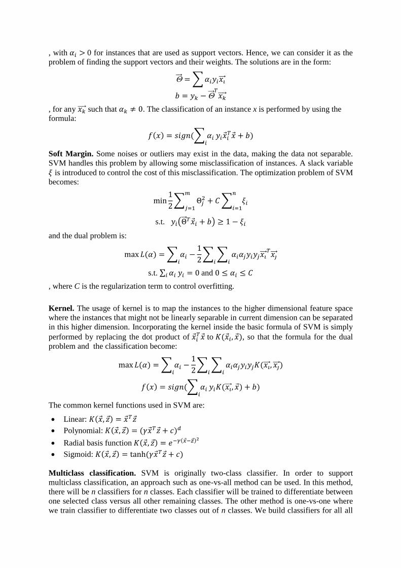
Decision Tree. A decision tree algorithm builds a single classification tree with each node

contains a question to decide of how to classify a given instance (Figure 2).

Figure 2 Illustration of Decision Tree. Instance x represented with two numerical features (x1, x2)

is classified as c1 or c2 based on the values of the features it has.

In building the tree, we first start with a single node. A node in the tree contains the

collection of instances from our training data. Node has a measure of impurity that intuitively

says that a node that contains high number of instances of the same classes (homogeneous)

has lower impurity compared to the node with instances of many different classes

(heterogeneous). Some formulas that are used to measure the degree of impurity in a node

are:

Misclassification error

Information gain (entropy)

∑ ( | )

Gini index

∑ ( | )

, where is the set of possible classes and ( | ) is a probability of class

given node . In ID3 algorithm, the instances in a node will be split into two different sets

(nodes) iteratively based on a single feature each time. The feature is selected so that the

decrease in impurity from parent to the children nodes is maximized.

𝑥

𝑥 class c1

class c1 class c2

x

, where and are left and right children nodes, and are the proportion of the

instances that go to the left and right nodes, and represents all possible splits. Hence, the

selected feature on each split will later be used as the question, to decide where an instance x

should go when performing classification. The split will continue until no more features to be

selected or if only one instance is left in the node. If necessary, a pruning can be performed to

stop the growth of the tree at certain stage to prevent overfitting.

Random Forests. As mentioned in the beginning of this section, Random Forests works by

constructing many classification trees. The class for an instance will be determined by

selecting class with majority votes. Each classification tree is build using the data sampled

from the training data with replacement. The size of sampled data can be less, as big as the

training data, or bigger. Using the total of M features, each tree will be constructed using

only m << M (far smaller) features, that are selected randomly. Tree will be grown without

pruning.

The basic idea in Random Forests that makes it a good classifier is that it is a collection of

the so-called weak learners, learning algorithms with low bias and high variance. The trees in

Random Forests are built to their maximum depth to produce low bias learners. The sampling

of data is performed to ensure the trees built have low correlation with each other. Using high

number of trees, the algorithm is claimed to not overfit.

The other important notion in Random Forests is out-of-bag data. The out-of-bag data is a

collection of instances that are not selected for building current classification tree. The

Random Forests calculate the out-of-bag error estimate from this data, i.e. out-of-bag data

acts as test data. The error estimate represents the overall averaged error estimate of the

classification. This value can be used to tune some parameters, e.g. choosing the m for the

features. It can also be used to rank variable importance by permuting the values of the

features in a single tree and calculating the increase in the misclassification rate averaged

over all the trees.

3.4 k-NN

The k-NN (k-nearest neighbor) algorithm is a member of instance-based learning algorithm.

Instance-based learning algorithm is a type of learners that is also called lazy learner. Given

training data, the instance-based learning algorithm will store the data and only use it when it

is needed to do the classification or regression. In the case of classification, the task is

performed by comparing the given test instance from test data with the instances from the

stored training data.

In k-NN method, the comparison is performed with the closest k neighbors in the training

data. The measure of distance used for finding the closest k neighbors might be varied.

Among them, the most commonly used is Euclidean distance. The Euclidean distance

between two instances x and y, where each instance is represented as a features vector of m

numerical features, is given by:

√∑

For classification, the label of the test instance will be labeled according to the majority class

of its k nearest neighbor.

∑

, where C is the set of all possible labels, is the label of the i-th neighbor of x, and

is 1 when c = ci and 0 otherwise. Finding which k nearest neighbor to be included can be

performed randomly. The other option is to include all the instances that have the same

distance with the k-th nearest vector.

4 Experiments and Results

We implemented our features extraction in Perl v5.14.2. The selection of features and

machine learning experiments was performed in R v2.15.1 and will be explained in Section

4.1. We will describe our experiment for each method that we chose in the following sections,

together with the tuning processes and the evaluation results. The overall process of our

experiments is depicted in Figure 3.

Figure 3 Overview of the experiments

We built features representation of all sentences using our 116 defined features. The

features were then converted into binary features. We split the data into two parts, training

and test data. The training data was used to perform two main steps, features selection and

parameters tuning. The final prediction was performed on the test data using the selected

features and parameters from the tuning process.

4.1 Feature Selection

The features were scored using FSelector package v0.18 in R that calculates the weight or

importance of each feature using Random Forests variable importance score. We show the

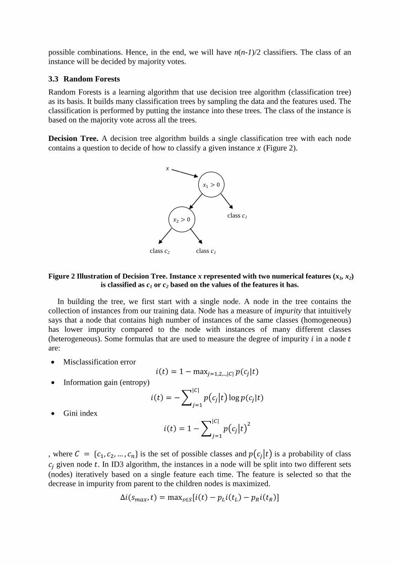
top 20 features for each word in Table 4.

Table 4 Top 20 features based on Random Forests variable importance measure

hard line serve

Feature Imp Feature Imp Feature Imp

TW_NEXT2_IN_at 34.13 TW_PHONE_BEFORE 54.33 TW_NSUBJ_DEP_P 42.24

All Data Training Data Testing Data

Features

Extraction

Features

Selection

Parameter

Tuning

(10 CV)

Prediction

(Final

accuracy)

Weight feature importance (Random

Forests)

Decide the number of

features to use (top N features) for each

method using 10 CV

SVM: cost, degree,

gamma

Random Forests:

number of trees, number of variable

sampling, node size

k-NN: number of neighbors

Prediction using the

best parameters for

each method

Extract 116 features (binary

and categorical)

Convert all

features to binary

features

TW_PREV1_NOM 32.36 TW_POSS_DEP_P 39.45 TW_PREP_AS_DEP_N 41.49

TW_ADVMOD 26.28 TW_DET_the 38.81 TW_NSUBJ 40.89

TW_PREV3_NOM 24.79 TW_COLON_AFTER 38.19 TW_TENSE_VBD 38.23

TW_PREV1_L_BE 23.88 TW_PREV1_NOM 35.74 TW_NEXT1_IN_as 37.66

TW_AMOD 23.57 TW_NN 33.82 TW_PREV1_WHP 37.04

TW_NEXT1_NOM 22.37 TW_PREV2_IN_NONE 32.13 TW_TENSE_VB 37.04

TW_PREV2_IN_on 19.92 TW_DET_NONE 31.63 TW_PREV1_NOM 36.65

TW_PREV2_TENSE_NONE 19.62 TW_PREV1_IN_in 31.55 TW_NEXT1_ADV 34.01

TW_NEXT2_VRB 19.35 TW_PREV2_ADV 30.51 TW_NSUBJ_DEP_N 33.49

TW_PREV2_VRB 19.34 TW_DET_a 30.33 TW_TENSE_VBG 32.90

TW_PREV1_ADV 18.79 TW_NEXT1_IN_between 29.83 TW_NEXT1_IN_by 32.73

TW_NEXT1_IN_for 18.76 TW_PREV2_IN_on 29.74 TW_NEXT2_NOM 32.49

TW_PREV1_IN_NONE 18.42 TW_NEXT1_IN_of 29.58 TW_NEXT1_IN_with 29.58

TW_NEXT2_ADV 18.41 TW_PREV1_ADJ 29.00 TW_DOBJ 29.26

TW_PREV3_VRB 18.25 TW_PREV2_IN_along 28.39 TW_PLURAL_OB 29.19

TW_NEXT2_TENSE_NONE 18.01 TW_PREP_BETWEEN 27.40 TW_OBJECT 28.13

TW_PREV2_L_BE 17.84 TW_PREV3_VRB 27.18 TW_PREV1_IN_NONE 26.93

TW_NEXT2_IN_NONE 17.81 TW_DOBJ_OF 26.90 TW_NEXT1_IN_NONE 26.90

TW_NEXT2_NOM 17.65 TW_PREV2_NOM 26.42 TW_PREV1_ADV 26.71

We can observe from the word “hard” that the important features are most likely in the

class of nominal (NOM), verb (VRB), adverb (ADV), and preposition or subordinating

conjunction (IN). As the word “hard” itself is an adjective, we can see that the presence of

feature related to the adjective class is not in the top 20 of the features. The presence of verb

and nominal is probably because an adjective usually describe word in verb and nominal

class, e.g. uses of “hard” as adverbial modifier or adjectival modifier. Some prepositions or

subordinating conjunction around the word “hard” like “at”, “on”, “for” seem to be important

in disambiguating the sense. The presence of lemma “be” (*_L_BE) is important probably

because we usually use the word “is”, “are” before an adjective. The non-occurrence of some

classes (*_NONE) is also important, especially for non-occurrence of preposition and word

with certain tenses.

For the word “line”, some of the features are quite specific. For example, the presence of

word related to phone as the top feature. This is probably due to the use of the cue words

listed in the feature TW_PHONE_BEFORE strongly disambiguate the sense of the word “line” as

“communication line (phone line)”. The presence of some specific determiners, prepositions,

and subordinating conjunction is also important in disambiguating the senses. The other

interesting things to see are the use of possessive dependency (TW_POSS_DEP_P) and the use of

colon “:”. Looking into the training data, these two features seem to relate to the use of word

“line” which has the sense of “text” or “quote” from someone.

In word “serve” the number of features related to the prepositions or subordinating

conjunction seems to be smaller compared to the word “hard” and “line”. Some important

words based on the feature’s score are “as”, “by”, “with”. These words when combined with

the word “serve” will be something like “serve by”, “serve as”, “serve with”, which help in

disambiguating the sense of the word “serve”. The prominent features are features that relate

to the subject, object, or the tense of the word “serve”. This is probably due to the nature of

the word “serve” as a verb.

Comparing these three top 20 features, we can get some rough conclusions of the

importance of features related to the class of word: “hard” as adjective, “line” as noun, and

“serve” as verb. For adjective, the presence of nominal and prepositions seem to have

important roles. For noun, some specific features are necessary to disambiguate its sense. As

for the verb, features related to function of words as subject or object are more important.

The feature selection was performed for each learning method. We selected top N best

features based on 10-fold cross validation and the average accuracy. We did not do cross

validation for Random Forests method, since the overall error estimate from out-of-bag data

should be representative enough in measuring the performance of the classifier. We used the

out-of-bag error estimation and selected the N that produces the lowest error estimation. For

each method, we set the N from 50 to 150 and increase it by 10 in each iteration. The N that

produces the highest average accuracy (or lowest error estimate for Random Forests) was

selected. The selected N for each learning method will be shown on the following sections as

“# Features”.

4.2 SVM

SVM is available in R under the library e1071 with the function named svm. The function

provides multliclass classification using one-against-one method. In SVM experiments, we

used all the kernels provided to compare the performance of different kernels to solve the

disambiguation problem. For each kernel, we tuned the related parameters using 10-fold cross

validation, performed by setting the parameter cross=10. We only tuned the parameters Cost,

Gamma, and Degree. All other parameters were not changed. We decided not to use

exhaustive search in tuning the parameters due to the time needed to do the exhaustive search.

We tuned the parameters by the order of: cost > gamma > degree. Cost will be the first to

tune. Afterwards, we set the cost for the SVM using the best cost obtained to search for the

best gamma. Degree will be searched the last using the best cost and the best gamma. The

possible values for each parameter are:

Cost: 1, 10, 100

Gamma: 0.01, 0.1, 1, 10, 100

Degree: 1, 2, 3, 4, 5

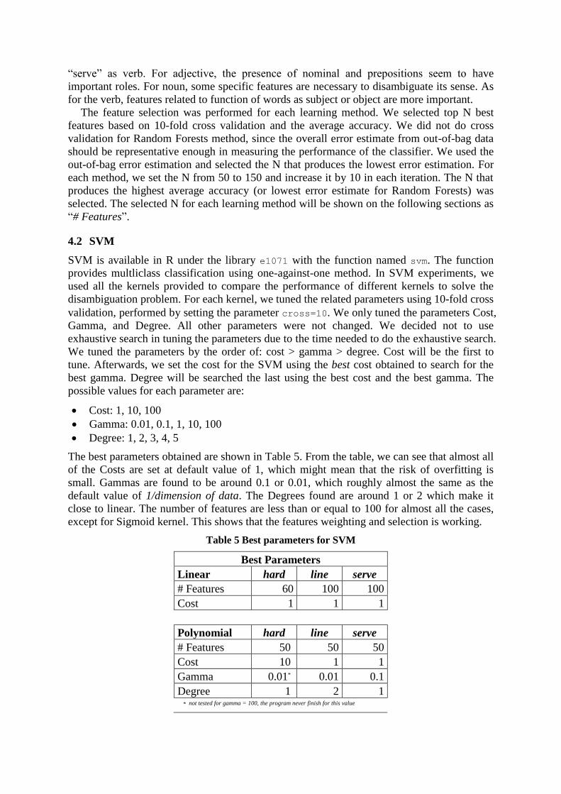
The best parameters obtained are shown in Table 5. From the table, we can see that almost all

of the Costs are set at default value of 1, which might mean that the risk of overfitting is

small. Gammas are found to be around 0.1 or 0.01, which roughly almost the same as the

default value of 1/dimension of data. The Degrees found are around 1 or 2 which make it

close to linear. The number of features are less than or equal to 100 for almost all the cases,

except for Sigmoid kernel. This shows that the features weighting and selection is working.

Table 5 Best parameters for SVM

Best Parameters

Linear hard line serve

# Features 60 100 100

Cost 1 1 1

Polynomial hard line serve

# Features 50 50 50

Cost 10 1 1

Gamma 0.01* 0.01 0.1

Degree 1 2 1

* not tested for gamma = 100, the program never finish for this value

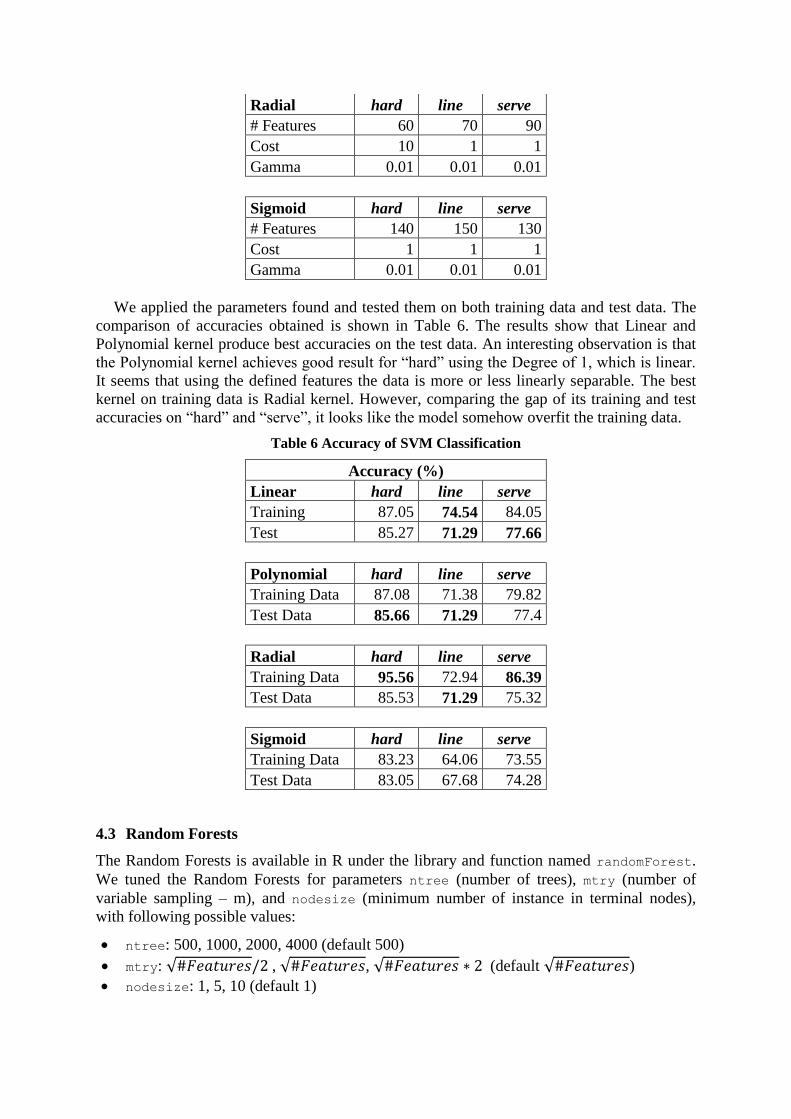
Radial hard line serve

# Features 60 70 90

Cost 10 1 1

Gamma 0.01 0.01 0.01

Sigmoid hard line serve

# Features 140 150 130

Cost 1 1 1

Gamma 0.01 0.01 0.01

We applied the parameters found and tested them on both training data and test data. The

comparison of accuracies obtained is shown in Table 6. The results show that Linear and

Polynomial kernel produce best accuracies on the test data. An interesting observation is that

the Polynomial kernel achieves good result for “hard” using the Degree of 1, which is linear.

It seems that using the defined features the data is more or less linearly separable. The best

kernel on training data is Radial kernel. However, comparing the gap of its training and test

accuracies on “hard” and “serve”, it looks like the model somehow overfit the training data.

Table 6 Accuracy of SVM Classification

Accuracy (%)

Linear hard line serve

Training 87.05 74.54 84.05

Test 85.27 71.29 77.66

Polynomial hard line serve

Training Data 87.08 71.38 79.82

Test Data 85.66 71.29 77.4

Radial hard line serve

Training Data 95.56 72.94 86.39

Test Data 85.53 71.29 75.32

Sigmoid hard line serve

Training Data 83.23 64.06 73.55

Test Data 83.05 67.68 74.28

4.3 Random Forests

The Random Forests is available in R under the library and function named randomForest.

We tuned the Random Forests for parameters ntree (number of trees), mtry (number of

variable sampling – m), and nodesize (minimum number of instance in terminal nodes),

with following possible values:

ntree: 500, 1000, 2000, 4000 (default 500)

mtry: √ , √ , √ (default √ )

nodesize: 1, 5, 10 (default 1)

All other parameters were not changed. The selection of best parameter was performed by

selecting the parameter that produces lowest error estimate of out-of-bag data over all the

trees, taken from the last index of err.rate value returned by the randomForest model. The

tuning is performed in the similar way as SVM with the order of search: ntree > mtry >

nodesize. The best parameters that we obtained are shown in Table 7.

From the table, we can see that the best node size is 1, which mean the trees can be grown

to the maximum depth. The numbers of features are varied with “serve” having the highest

number of features. Small number of features is apparently enough for word “hard”. The

number of trees, however, is the largest for word “hard”, set at the maximum of possible

values. The forest for “hard” takes small number of variable sampling but uses many trees to

achieve good performance. For “serve”, the number of variable sampling is higher but with

smaller number of trees. The word “line” use small number of trees (default) with small

number of variable sampling.

Table 7 Best parameters for Random Forests

Best Parameters

Random Forests hard line serve

# Features 50 100 140

Number of trees 4000 500 1000

Variable sampling 7 10 24

Node size 1 1 1

Accuracies for each word are shown in Table 8. The results show a big discrepancy

between the accuracy on training data and on the testing data. The accuracy on the training

data is on average around 90% or higher. However, the accuracy on the test data only lies

around 70%-80%. Observing the discrepancy, we see that the gaps are large for word “line”

and “serve”. This might be related to the smaller number of trees used compared to “hard”.

Increasing the number of trees might be able to decrease the discrepancy, but probably will

not produce better accuracy.

Table 8 Accuracy of Random Forests Classification

Accuracy (%)

Random Forests hard line serve

Training Data 90.41 89.04 97.89

Test Data 84.35 73.23 79.87

4.4 k-NN

Implementation of k-NN method is available in R under library e1071 with the function

named knn. We only tuned for one parameter k (number of neighbor), as this is the only one

that we think is important to tune. The tuning was based on the average accuracy of 10-fold

cross validation on the training data. For k-NN, the values for # Features is set higher to be

from 100 to 190. Smaller number of features might not generalize enough and using higher

number might better distinguish one instance from the others. The results are shown in

TABLE 9.

We see from the results that using 100 features is enough for “hard”, but for “line” and

“serve” higher number of features is preferred. Setting the k to be 1 and 2 seems to be enough

for “hard” and “serve”. The instances in these two words might be distinguishable enough, so

that one neighbor is sufficient to achieve best accuracy. For word “line”, higher number of

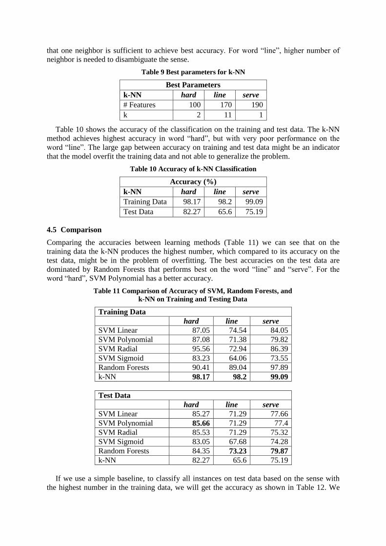
neighbor is needed to disambiguate the sense.

Table 9 Best parameters for k-NN

Best Parameters

k-NN hard line serve

# Features 100 170 190

k 2 11 1

Table 10 shows the accuracy of the classification on the training and test data. The k-NN

method achieves highest accuracy in word “hard”, but with very poor performance on the

word “line”. The large gap between accuracy on training and test data might be an indicator

that the model overfit the training data and not able to generalize the problem.

Table 10 Accuracy of k-NN Classification

Accuracy (%)

k-NN hard line serve

Training Data 98.17 98.2 99.09

Test Data 82.27 65.6 75.19

4.5 Comparison

Comparing the accuracies between learning methods (Table 11) we can see that on the

training data the k-NN produces the highest number, which compared to its accuracy on the

test data, might be in the problem of overfitting. The best accuracies on the test data are

dominated by Random Forests that performs best on the word “line” and “serve”. For the

word “hard”, SVM Polynomial has a better accuracy.

Table 11 Comparison of Accuracy of SVM, Random Forests, and

k-NN on Training and Testing Data

Training Data

hard line serve

SVM Linear 87.05 74.54 84.05

SVM Polynomial 87.08 71.38 79.82

SVM Radial 95.56 72.94 86.39

SVM Sigmoid 83.23 64.06 73.55

Random Forests 90.41 89.04 97.89

k-NN 98.17 98.2 99.09

Test Data

hard line serve

SVM Linear 85.27 71.29 77.66

SVM Polynomial 85.66 71.29 77.4

SVM Radial 85.53 71.29 75.32

SVM Sigmoid 83.05 67.68 74.28

Random Forests 84.35 73.23 79.87

k-NN 82.27 65.6 75.19

If we use a simple baseline, to classify all instances on test data based on the sense with

the highest number in the training data, we will get the accuracy as shown in Table 12. We

can see that for the word “hard”, the baseline accuracy is already high. However, all of the

learning methods that we used have higher accuracies compared to the baseline.

Table 12 Baseline accuracy using majority class in training data

to classify test data

Accuracy (%)

Baseline hard line serve

SVM Linear 78.10 56.45 40.26

We performed paired student’s t-test to see whether one method is hypothetically better

than the other. We compared four methods: SVM Polynomial, Random Forests, k-NN, and

the baseline. SVM with polynomial kernel is chosen as representative of the SVM method

since it produces better accuracies compared to the other methods, although, linear kernel is

also possible. The paired t-test was performed on each word separately. The accuracy for

each method and word was calculated on 10-fold data taken from test data. The results are

shown in Table 13.

Table 13 Accuracy of each method on 10-fold data

Accuracy (%)

hard line serve

No SVM RFS KNN BAS SVM RFS KNN BAS SVM RFS KNN BAS

1 85.71 83.12 77.92 76.62 62.50 65.28 55.56 54.17 75.32 75.32 70.13 37.66

2 83.12 77.92 75.32 83.12 65.28 68.06 61.11 47.22 81.82 84.42 68.83 49.35

3 87.01 90.91 83.12 84.42 75.00 70.83 65.28 65.28 72.73 79.22 70.13 32.47

4 87.01 85.71 80.52 77.92 70.83 65.28 61.11 62.50 63.64 64.94 55.84 38.96

5 80.52 81.82 79.22 79.22 61.11 72.22 68.06 61.11 74.03 75.32 67.53 36.36

6 76.62 81.82 71.43 68.83 62.50 66.67 56.94 48.61 76.62 81.82 71.43 51.95

7 76.62 75.32 74.03 68.83 62.50 69.44 61.11 56.94 66.23 68.83 59.74 36.36

8 81.82 80.52 72.73 74.03 69.44 66.67 62.50 58.33 74.03 70.13 63.64 33.77

9 85.71 87.01 80.52 80.52 58.33 56.94 51.39 48.61 80.52 76.62 76.62 42.86

10 82.43 87.84 77.03 87.84 82.19 83.56 71.23 61.64 77.92 75.32 71.43 42.86

* RFS: Random Forests, BAS: baseline

We use function t.test in R with the parameter paired set to True. The significance

level is set to 0.05. The H0 for the test is: the true difference in means between the two

methods is 0. If the p-value from the test is greater than , we will reject the null hypothesis.

The results are shown in Table 14.

Table 14 The p-values for paired student’s t-test

Comparison p-value

hard line serve

SVM-BAS 0.01544 0.00032 0.00000

RFS-BAS 0.00986 0.00021 0.00000

KNN-BAS 0.55268 (r) 0.00861 0.00000

SVM-RFS 0.63753 (r) 0.37538 (r) 0.44172 (r)

SVM-KNN 0.00006 0.00844 0.00006

RFS-KNN 0.00025 0.00003 0.00026 *(r): reject H0

We can see that for the word ”hard”, we cannot reject H0 that the mean accuracies of k-NN

is equal to the mean accuracy of the baseline. Hence, for this word, k-NN does not perform

better than baseline. Another interesting thing is that we accept the H0 that the mean

difference in accuracy for SVM Polynomial and Random Forests is equal to 0, i.e. SVM

Polynomial and Random Forests has same performance over all the words. For other cases,

we can see that SVM, Random Forests, and k-NN are better than baseline, with k-NN

concluded to be the lowest.

5 Conclusions

We compared three machine learning methods, SVM, Random Forests, and k-NN, to perform

word sense disambiguation task on word “hard”, “line”, and “serve”. We performed the

feature scoring and selection to rank the features by their importance. The top 20 features

show interesting outlook that each word has different kind of features that best suit them.

Comparing all the methods, we concluded that Random Forests and SVM has the best

accuracy with more or less the same performance. The k-NN method performs lower than the

other two methods and only better than baseline on the word “line” and “serve”.

References

Cutler, Leo Breiman and Adele. Random Forests. n.d. 16 February 2013.

<http://www.stat.berkeley.edu/~breiman/RandomForests/cc_home.htm>.

—. Visualizing Random Forests. n.d. 2013 February 16.

<http://www.stat.berkeley.edu/~breiman/RandomForests/ENAR_files/frame.htm>.

Fellbaum, Christiane. "WordNet: An Electronic Lexical Database." (1998).

k-Nearest Neighbour Classification. n.d. 11 February 2013. <http://stat.ethz.ch/R-manual/R-

patched/library/class/html/knn.html>.

Leacock, C. and Miller, G.A. and Chodorow, M. "Using corpus statistics and WordNet

relations for sense identification." Computational Linguistics 24 (1998): 147-165.

Manning, C.D. and Raghavan, P. and Schutze, H. Introduction to information retrieval. Vol.

1. Cambridge University Press Cambridge, 2008.