Within subjects t testsWithin subjects t tests

• Related samplesRelated samples

• Difference scoresDifference scores

• tt tests on difference scores tests on difference scores

• Advantages and disadvantagesAdvantages and disadvantages

Related SamplesRelated Samples

• The same participants give us data on The same participants give us data on two measurestwo measures e. g. Before and After treatmente. g. Before and After treatment

Usability problems before training on PP and Usability problems before training on PP and after trainingafter training

• With related samples, someone high on With related samples, someone high on one measure probably high on one measure probably high on other(individual variability).other(individual variability).

Cont.

Related Samples--cont.Related Samples--cont.

• Correlation between before and Correlation between before and after scoresafter scores Causes a change in the statistic we can Causes a change in the statistic we can

useuse

• Sometimes called matched samples Sometimes called matched samples or repeated measuresor repeated measures

Difference ScoresDifference Scores

• Calculate difference between first Calculate difference between first and second scoreand second score e. g. Difference = Before - Aftere. g. Difference = Before - After

• Base subsequent analysis on Base subsequent analysis on difference scoresdifference scores Ignoring Before and After dataIgnoring Before and After data

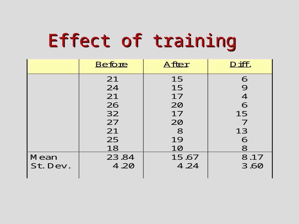
Effect of training Effect of training Before After Diff.

21 24 21 26 32 27 21 25 18

15 15 17 20 17 20 8

19 10

6 9 4 6

15 7

13 6 8

Mean St. Dev.

23.84 4.20

15.67 4.24

8.17 3.60

ResultsResults

• The training decreased the number of The training decreased the number of problems with Powerpointproblems with Powerpoint

• Was this enough of a change to be Was this enough of a change to be significant?significant?

• Before and After scores are not Before and After scores are not independent.independent. See raw dataSee raw data

rr = .64 = .64

Cont.

Results--cont.Results--cont.

• If no change, mean of differences If no change, mean of differences should be zeroshould be zero So, test the obtained mean of So, test the obtained mean of

difference scores against difference scores against = 0. = 0.

Use same test as in one sample testUse same test as in one sample test

tt test test

85.62.1

22.8

9

6.322.8

n

sD

tD

D and sD = mean and standard deviation of differences.

df = n - 1 = 9 - 1 = 8

Cont.

tt test--cont. test--cont.

• With 8 With 8 dfdf, , tt.025.025 = = ++2.306 (Table E.6)2.306 (Table E.6)

• We calculated We calculated tt = 6.85 = 6.85

• Since 6.85 > 2.306, reject Since 6.85 > 2.306, reject HH00

• Conclude that the mean number of Conclude that the mean number of problems after training was less problems after training was less than mean number before trainingthan mean number before training

Advantages of Related Advantages of Related SamplesSamples

• Eliminate subject-to-subject Eliminate subject-to-subject variabilityvariability

• Control for extraneous variablesControl for extraneous variables

• Need fewer subjectsNeed fewer subjects

Disadvantages of Related Disadvantages of Related SamplesSamples

• Order effectsOrder effects

• Carry-over effectsCarry-over effects

• Subjects no longer naïveSubjects no longer naïve

• Change may just be a function of timeChange may just be a function of time

• Sometimes not logically possibleSometimes not logically possible

Between subjects t testBetween subjects t test

• Distribution of differences between Distribution of differences between meansmeans

• Heterogeneity of VarianceHeterogeneity of Variance

• NonnormalityNonnormality

Powerpoint training againPowerpoint training again

• Effect of training on problems using Effect of training on problems using PowerpointPowerpoint Same study as before --almostSame study as before --almost

• Now we have two independent Now we have two independent groupsgroups Trained versus untrained usersTrained versus untrained users We want to compare mean number of We want to compare mean number of

problems between groupsproblems between groups

Effect of training Effect of training Before After Diff.

21 24 21 26 32 27 21 25 18

15 15 17 20 17 20 8

19 10

6 9 4 6

15 7

13 6 8

Mean St. Dev.

23.84 4.20

15.67 4.24

8.17 3.60

Differences from within Differences from within subjects testsubjects test

Cannot compute pairwise differences, since we cannot compare two random people

We want to test differences between the two sample means (not between a sample and population)

AnalysisAnalysis

• How are sample means distributed How are sample means distributed if if HH00 is true? is true?

• Need sampling distribution of Need sampling distribution of differences between meansdifferences between means Same idea as before, except statistic is Same idea as before, except statistic is

(X(X11 - X - X22) (mean 1 – mean2)) (mean 1 – mean2)

Sampling Distribution of Sampling Distribution of Mean DifferencesMean Differences

• Mean of sampling distribution = Mean of sampling distribution = 11 - - 22

• Standard deviation of sampling Standard deviation of sampling distribution (standard error of mean distribution (standard error of mean differences) = differences) =

2

2

2

1

2

121 n

sns

sXX

Cont.

Sampling Distribution--Sampling Distribution--cont.cont.

• Distribution approaches normal as Distribution approaches normal as nn increases.increases.

• Later we will modify this to “pool” Later we will modify this to “pool” variances.variances.

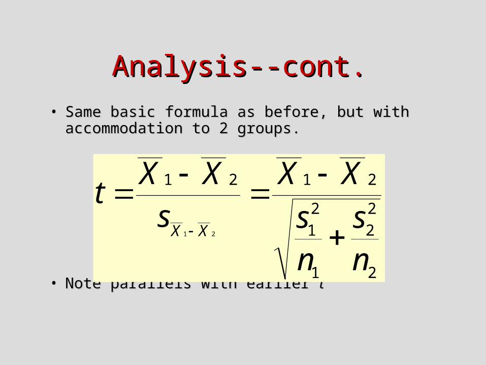
Analysis--cont.Analysis--cont.

• Same basic formula as before, but with Same basic formula as before, but with accommodation to 2 groups.accommodation to 2 groups.

• Note parallels with earlier Note parallels with earlier tt2

2

2

1

2

1

2121

21

ns

ns

XXsXX

tXX

Degrees of FreedomDegrees of Freedom

• Each group has 6 subjects. Each group has 6 subjects.

• Each group has Each group has nn - 1 = 9 - 1 = 8 - 1 = 9 - 1 = 8 dfdf

• Total Total dfdf = = nn11 - 1 + - 1 + nn22 - 1 = - 1 = nn11 + + nn22 - 2 - 2

9 + 9 - 2 = 16 9 + 9 - 2 = 16 dfdf

• tt.025.025(16) = (16) = ++2.12 (approx.)2.12 (approx.)

ConclusionsConclusions

• T = 4.13T = 4.13

• Critical t = 2.12Critical t = 2.12

• Since 4.13 > 2.12, reject Since 4.13 > 2.12, reject HH00..

• Conclude that those who get Conclude that those who get training have less problems than training have less problems than those without training those without training

AssumptionsAssumptions

• Two major assumptionsTwo major assumptions Both groups are sampled from Both groups are sampled from

populations with the same variancepopulations with the same variance• ““homogeneity of variance”homogeneity of variance”

Both groups are sampled from normal Both groups are sampled from normal populationspopulations• Assumption of normalityAssumption of normality

Frequently violated with little harm.Frequently violated with little harm.

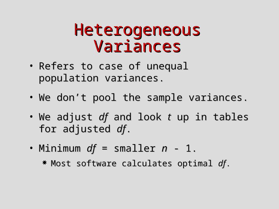
Heterogeneous VariancesHeterogeneous Variances

• Refers to case of unequal population Refers to case of unequal population variances.variances.

• We don’t pool the sample variances.We don’t pool the sample variances.

• We adjust We adjust dfdf and look and look tt up in tables for up in tables for adjusted adjusted dfdf..

• Minimum Minimum dfdf = smaller = smaller nn - 1. - 1. Most software calculates optimal Most software calculates optimal dfdf..