Proceedings of the Turin Royal Academy of Science

Vol. 79, 1944

WIRE ROPE BENDING

STIFFNESS FACTORS By Modesto Panetti Introduction and translation from Italian

by Alain Cardou, Ph.D.

i

WIRE ROPE BENDING

STIFFNESS FACTORS

By

Modesto Panetti

Translated from Italian

by Alain Cardou, Ph.D.

2015

ii

MODESTO PANETTI (1875-1957)

An Italian engineer, he became Applied Mechanics professor in Genoa and, later, in Torino. Member

of the Turin Academy of Science, of the Papal Academy of Science, and corresponding member of the

“Accademia dei Lincei” (of which Academy Galileo Galilei was an early member). A Senator and also

Minister of Postal Service and Telephone after World War II

FOREWORD

Helical strand mechanics may apply to such practical systems as cables and overhead electrical

conductors. In a 1997 review paper, Cardou and Jolicoeur summarized current available models1 . In

2006, this review has been updated by Cardou, at least for the bending stiffness problem2.

In the latter, several early contributions were mentioned, which had been “forgotten” in the 1997

review. Among them, a paper by Panetti (1944), published in Italian and, probably for that reason,

completely ignored in the later technical literature. The translation given below strives to redress as

much as possible this “injustice”.

Of course, one may wonder if Panetti’s results are still relevant. In recent years, several studies have

been published which were based on the Finite Element method. In general, they deal with the

relatively simple axial load problem. A multilayer strand in bending is much more complex a problem,

involving multiple contact points (at least for cross-lay strand), friction, partial slip etc. Thus, a

numerical treatment will obviously necessitate a number of simplifying assumptions. For that reason,

an analytical approach is still of interest.

Analytical models also require a number of assumptions, and Panetti’s are not immune to criticism,

such as his hypothesis of “circumferential” or same layer contact between wires. However, his uniform

curvature bending stiffness theory yields, at least qualitatively, similar results to more recent models.

Panetti’s paper can therefore be read with interest by anyone working on a new model of helical strand

mechanics. In any case, it should deserve proper credit through its inclusion in relevant lists of

references.

A.C.

1 Cardou, A., and Jolicoeur, C., Mechanical models of helical strands, Applied Mechanics Reviews, Vol. 50, No 1, pp. 1-14.

2 Cardou, A., Taut helical strand bending stiffness, available on line at www.umformtechnik.net. 9 pages

- 1 -

WIRE ROPE BENDING STIFFNESS FACTORS

A presentation3 by Modesto Panetti

(Member of the Academy)

Presented at the 23 February 1944 Meeting

ABSTRACT

First, cable geometry is presented. Then, interwire pressure arising from the applied axial load is

derived. It is based on the “circumferential contact” assumption, as opposed to the more widely used

“radial contact” assumption, which was used even by the Author himself in a previous paper on the

same subject.

This assumption yields a simpler calculation of friction work occurring in a taut cable in bending,

where the limit case of inextensible wire is made, and also that of bending tensile forces, whose

determination is based on the theoretical case of a uniform curvature.

This approach allows a separate study of the stiffness factors and of bent cable debonding from the

cable bending details, such as its deformed curve geometry, as they appear in previous papers by

Findeis and Hellmut Ernst.

This presentation concludes by deriving a relationship between curvature and resisting internal

moments. The corresponding equation might be of some practical interest in applications.

INTRODUCTION

If curvature is imposed onto a wire rope under axial load, supplementary forces are generated in

individual wires. Depending on the location of a wire section with respect to the cable neutral axis, they

add up or subtract from the initial wire tensile force.

At the same time, tangential forces are generated between contacting wires. They arise from two

separate phenomena.

Firstly, they will come from the variation of cable curvature along its axis. It is equivalent to shear

stress generation in a solid beam in bending.

Secondly, they arise from the helical winding of wires, even under uniform curvature. For a taut cable,

such a uniform curvature may be achieved only by supporting the cable onto a rigid saddle. This

hypothesis will be made, thus eliminating the first effect from the problem.

3 M. Panetti, I fattori della rigidezza delle funi metalliche , Atti dalla Reale Accademia delle Scienze di Torino, Cl. di

Scienze fisiche, Vol. 79, 1944, pp. 1-37

- 2 -

There is an upper limit on tangential forces since slip may occur once that limit is reached. For a given

wire, slip occurs within the cable in the same direction as if it were inextensible.

For a given wire element, slip direction is such that, because of symmetry, wire sections located at

extreme positions, that is, inside (concave side) and outside (convex side) of a torus, should not slip.

Tangential force directions are directly related to these displacements, and they act opposite to slip

direction.

Besides, tangential forces are made possible because of interwire pressure. Two limit cases are to be

considered: either purely radial pressure transmission from one layer to the next; or purely

circumferential (lateral) transmission between same layer wires.

In fact, in practical cases, these two modes probably coexist, one of them prevailing over the other,

depending on cable geometrical parameters.

However, using one or the other of these limit hypotheses leads to opposite conclusions on tangential

force distribution.

Indeed, between two wires belonging to adjacent layers or, more exactly, between the outer and inner

layer, their relative slip motion is in the direction away from the neutral axis; thus, the tangential force

on the outer wire is directed towards the neutral axis.

As the tensile force increments acting at both ends of the wire element are in opposite directions,

tangential forces must decrease further away from the neutral axis, as in solid beams in bending.

If, on the contrary, one considers wires belonging to the same layer, displacement of an element further

away from the neutral axis slips with respect to the element closest to the neutral axis in such a way as

to get closer to the neutral axis. As in the previous case, a wire element is subjected to a force

increment away from the neutral axis. Equilibrium of the element requires that tangential forces will

also increase in that direction, which is the opposite of what happens in solid beams in bending.

Slip leads to some wire debonding within the cable. According to hypothesis No 1, debonding occurs

from outer to inner layers; and, in a given layer, from wires closest to the neutral axis to those further

away, With hypothesis No 2, slip occurs first between wires further away and extends progressively to

wires closer to neutral axis.

This process corresponds to a loss in mechanical energy, and, correspondingly, to the work of a friction

internal moment. Besides, when debonding is complete, elastic cable resistance to bending is a

minimum corresponding to the bending stiffness of wires acting independently.

This work begins with a study of cable geometry. It leads to a relationship between interwire pressure

and applied axial load. Here, it is assumed, and is considered as most probable, that contact mode is

circumferential rather than radial. The latter assumption has been widely used in earlier works,

including by the Author in a paper on the same topic which has been published in 1909 in this

Academy’s Transactions under the title “Wire rope elastic modulus under axial load.”

This contact mode assumption makes it simpler the evaluation of friction work occurring in cable

bending, using the limit case of inextensible wires, as well as the calculation of wire tensile forces

- 3 -

resulting from the curvature (called bending forces). Besides, uniform curvature is assumed, which

leads to a simple relationship between curvature and bending moment.

This approach makes it possible to separate stiffness modulus evaluation and cable debonding process

from the details of cable bending, i.e. from its deformed curve particular geometry, such as the one in

Hellmut Ernst’s work4. Consequently, his results are rather different from those reported in the present

paper.

1. Wire geometry

In preparation for the subsequent analysis, the basic equations of a circular helix are recalled. Calling α

the lay angle with respect to the cable axis and r the radius of the lay cylinder, helix pitch p, or lay

length, is given by:

p 2 r cot= π α (1)

Given α, pitch increases with each layer mean radius.

Going from one layer to the next, with radius increasing, the number of wires increases by 6, while that

layer mean radius r increment is practically equal to wire diameter δ. Indeed, perimeters of two

adjacent layers mean circles differ by:

2 12 (r r ) 2- =π πδ (2)

Assuming that on the inner layer, wires are in contact, there will be some gap between those of the

outer layer, that gap resulting from the difference between 2π and 6.

However, considering a cable cross-section, wire cross-sections are practically ellipses having a semi-

major axis / cosδ α . Such axis is tangent to the layer mean circle, which goes through wire section

center points. Assume now that the mean circle perimeter is practically equal to the circumscribed

polygon perimeter; calling z the number of wire in each layer, one gets:

1 1 2 22 r z / cos 2 r z / cos= =π δ α π δ α

Letting 2 1z z 6- = , Eq. (2) yields :

6 2 cos= π α (3)

yielding 17= °α (approximately).

Thus, a lay angle of 17° is such that, in a given layer, wires are tightly wound. Such a lay is called

“normal”.

4 Beitrag zur Beurteilung der behördlichen Vorschriften für die Seilen von Personenschwebebahnen, in Fördertechnik und

Frachtverkehr, 1933, No 19 to 26 and 1934, No 3 to 7.

- 4 -

When laid at a smaller angle, there will be a gap between outer layer wires. If the angle is larger than

17° , there should be a gap between layers, which is prevented by wire deformation at points of

contact.

It has been shown that helical pitch differs in adjacent layers. This precludes the possibility that outer

wires fall in the troughs corresponding to contacting inner wires, even as the outer wires tend to align

themselves with the inner ones. Thus, the outer wires will cross over the inner ones like small bridges

and, for a constant curvature, they should keep their regular setting.

Frequency of these cross-over is easily derived. Indeed, distance between two same layer neighbouring

wires is / sinδ α when projected onto cable axis direction. Using Eqs (1) and (2), it is found that this

distance is related to the pitch difference between adjacent layers by:

2 1(p p ) 2 cossin

- ¸ =δ

π αα

From Eq. (3), for a normal lay, there must be 6 cross-over for a complete wire loop. Distance between

two cross-over is thus given by :

1 p

6 cosα

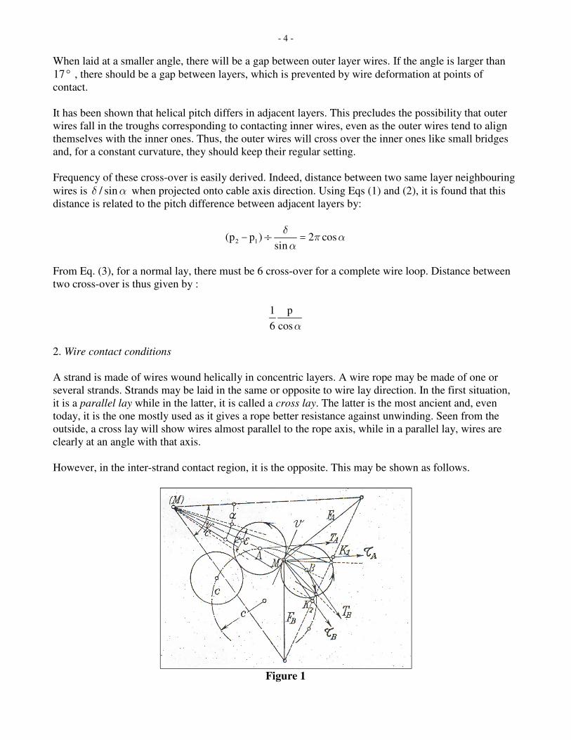
2. Wire contact conditions

A strand is made of wires wound helically in concentric layers. A wire rope may be made of one or

several strands. Strands may be laid in the same or opposite to wire lay direction. In the first situation,

it is a parallel lay while in the latter, it is called a cross lay. The latter is the most ancient and, even

today, it is the one mostly used as it gives a rope better resistance against unwinding. Seen from the

outside, a cross lay will show wires almost parallel to the rope axis, while in a parallel lay, wires are

clearly at an angle with that axis.

However, in the inter-strand contact region, it is the opposite. This may be shown as follows.

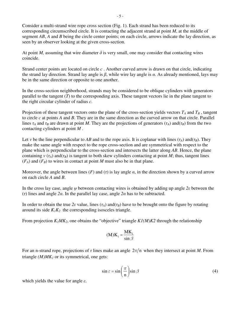
Figure 1

- 5 -

Consider a multi-strand wire rope cross section (Fig. 1). Each strand has been reduced to its

corresponding circumscribed circle. It is contacting the adjacent strand at point M, at the middle of

segment AB, A and B being the circle center points; on each circle, arrows indicate the lay direction, as

seen by an observer looking at the given cross-section.

At point M, assuming that wire diameter δ is very small, one may consider that contacting wires

coincide.

Strand center points are located on circle c . Another curved arrow is drawn on that circle, indicating

the strand lay direction. Strand lay angle is β, while wire lay angle is α. As already mentioned, lays may

be in the same direction or opposite to one another.

In the cross-section neighborhood, strands may be considered to be oblique cylinders with generators

parallel to the tangent (T) to the corresponding axis. These tangent vectors lie in the plane tangent to

the right circular cylinder of radius c.

Projection of these tangent vectors onto the plane of the cross-section yields vectors TA and TB , tangent

to circle c at points A and B. They are in the same direction as the curved arrow on that circle. Parallel

lines τA and τB are drawn at point M. They are the projections of generators (τA) and(τB) from the two

contacting cylinders at point M .

Let v be the line perpendicular to AB and to the rope axis. It is coplanar with lines (τA) and(τB). They

make the same angle with respect to the rope cross-section and are symmetrical with respect to the

plane which is perpendicular to the cross-section and intersects the latter along AB. Hence, the plane

containing v (τA) and(τB) is tangent to both skew cylinders contacting at point M; thus, tangent lines

(FA) and (FB) to wires in contact at point M must also be in that plane.

Moreover, the angle between lines (F) and (τ) is lay angle α, in the direction shown by a curved arrow

on each circle A and B.

In the cross lay case, angle ψ between contacting wires is obtained by adding up angle 2ε between the

(τ) lines and angle 2α. In the parallel lay case, angle 2α has to be subtracted.

In order to obtain the true 2ε value, lines (τA) and(τB) have to be brought onto the figure by rotating

around its side K1K2 the corresponding isosceles triangle.

From projection K1MK2, one obtains the “objective” triangle K1(M)K2 through the relationship

11

MK(M)K

sin=

β

For an n-strand rope, projections of τ lines make an angle 2 nπ when they intersect at point M. From

triangle (M)MK1 or its symmetrical, one gets:

sin sin sinn

æ öç ÷= ç ÷è ø

πε β (4)

which yields the value for angle ε.

- 6 -

Depending on the type of lay, cross or parallel lay, angle between contacting wires is given by:

c p2( ) 2( )ψ ε α ψ ε α= + = - (5)

For example, for a 6-strand rope, with a 17° lay angle, these equations yield:

c p30 8 25 50 50 (17 10 )n

πε ψ ψ¢ ¢ ¢= = - = - = - -� � � �

These results show clearly the difference between both types of lay and they also show why parallel lay

is preferred when a rope is under cyclic bending.

In fact, the larger angle between contacting wires in cross-lay rope will indeed increase their wear rate.

3. Compact and hollow strands

Strand structure also depends on wire distribution within the cross-section. In the compact case, total

number of wires is Z, giving a strand diameter d. Usually, Z is the sum of the base-6 series:

z 6 2 6 3 6 i 6= ´ ´ ´

and the corresponding radius of each layer is :

r 2 3 i= ´δ δ δ δ

Last term i is such that :

(2i 1) d+ =δ (6)

Hence :

2 2

2

d 3 dZ 6(1 2 3 )

2 4…

- -= + + + + =

δ δ

δ δ (7)

Adding up the strand core wire, a very good approximate value for Z is given by:

2

2

3 dZ

4=δ

(8)

Instead, for a hollow strand, that is, a strand with a textile or hemp core of diameter d1, wire number Z

is given by:

2 2

1

2

d d3Z

4

-=

δ (9)

Define now an “average” strand radius rm as follows:

- 7 -

m 1 1 2 2 3 3Zr z r z r z r …= + + + (10)

where z1, z2 etc. are the number of wires in layers of radius r1, r2 etc.

With the above values for z and r, they yield:

2

mZr 6 (1 4 9 i ) i(i 1)(2i 1)…= + + + + = + +δ δ (11)

As for a hollow strand, from Eq. (6):

11

ddi i

2 2

--= =

δδ

δ δ

Hence :

11

d di i

2

-- =

δ

Finally, using the Z value given either by Eq. (7) (compact strand), or Eq. (9) (hollow strand), the

respective average radius value follows:

3 3

1 1m m 2 2

1

d dd 1r r

3 3 d d

-= =

- (12)

In the second equation, a δ2.term has been neglected.

4. Strand “self-equilibrium” condition

A basic strand characteristic is the interwire pressure, which results from their helical shape and from

the tensile force t acting on each one of them.

An helical wire, curvature 2sin / rα , under tensile force t, must undergo a distributed normal force n,

per unit length, given by:

2 2t 2 1n sin t sin

r z= =

πα α

δ (13)

In a given layer, consider the product:

22zn t sin=

πα

δ (14)

Assuming the same lay angle, this product is the same for all layers. It is the strand “self-equilibrium”

condition.

- 8 -

Two limit cases may be considered regarding the way the normal force n is applied: it may result from

lateral contact between same layer wires, or else, it is applied radially, from one layer to the next, down

to the core wire.

Figure 2

With the first hypothesis, force n is the sum of two normal forces N (Fig. 2), coming from neighboring

wires. In that direction, radius of curvature of trajectory e, normal to wire axis, is 2r / cos α . Hence,

angle between lines through adjacent wire centers, that is, angle between forces N, is 2cos / r×δ α .This

yields :

2 2cos tan

2Nsin n that is : N t2r

δ α α

δ

æ ö×ç ÷ = = ×ç ÷è ø

(15)

where it is assumed that the sine value is equivalent to the angle.

Force N is independent of wire location within the strand, and the number of forces N to be considered

is equal to the number Z of wires within the strand.

With the second hypothesis, and numbering the layers from the outer one, it will be noticed that,

passing from layer 1 to layer 2, one should consider globally the zn forces given by Eq. (14), whose

total value, from Eq. (15), is 2πN, that is 6N approximately, letting cos 1α@ .

Layer 2 is also under a radial pressure equal to 6N to which must be added a pressure exerted on it by

layer 1. Thus, total pressure exerted by layer 2 is 12N.

The same approach being used from one layer to the next, radial pressure between layers is given by

the following series:

- 9 -

st nd nd rd rd th th th1 2 2 3 3 4 (i 1) i

6N 12N 18N (i 1)6N

® ® ® - ®

-

…

If the innermost layer (number i) is a 6-wire layer wound on a core wire, pressure between layer i and

core is iN, as for a 6-wire layer, n and N are equal, since r δ= .

Total is still ZN. Indeed, ( )6 1 2 3 i 3i(i 1) Z+ + + + = + =… , total number of wires in strand.

However, one gets the same result, even if the calculation stops at any inner layer i . Such layer

comprises ( )Z 6 i 1- - wires. It is acted on by radial load i× n and, according to Eq. (15), this is

transformed to i× N through tangential forces from the last layer.

In fact, taking the sum yields:

[ ] [ ] [ ]6N 1 2 3 (i 1) Z 6(i 1) iN iZ 3i(i 1) N…+ + + + - + - - = - -

where force N is still multiplied by total number Z.

Hence, taking either hypothesis, radial or lateral wire contact, total pressure between wires in a strand

is given by the same value ZN.

In practice, pressure transmission will follow an intermediate pattern, between radial and lateral,

depending on the degree of compactness of same layer wires. This depends on the layer lay angle: an

angle greater than the normal angle leading to more lateral contact, while a lay angle smaller than the

normal angle leads to more radial contact.

In fact, contact forces determination is a statically undetermined problem. A solution would require

calculation of contact deformations, assuming elastic behaviour; because interlayer contacts are point

contacts (Section 1) radial compliance is obviously greater than lateral compliance. It is thus logical to

assume that lateral contact is the prevailing mode.

This contact mode is such that outer layer wires are locked in place which is advantageous in the case

of a wire break.

Besides, in the radial contact mode, wires are subjected to bending between supporting contact points

(distance between neighboring contacts has already been given), thus increasing metal fatigue

problems.

It will be assumed that, even for a mixed contact mode, resultant of internal forces is the same as the

one found in the limit cases. Hence:

2 2tan T tan

ZN Ztcos

= =α α

δ α δ (16)

in which T is the total traction force on the cable. This so-called “self-locking” condition depends

directly on T through a constant factor. Assuming that cos 1α@ , this factor is practically 2sin /α δ , as

with a single wire.

- 10 -

However, even if the self-locking condition is the same, the contact mode, either lateral or radial, is not

without consequence on bending stiffness. This is shown in the sequel.

Actually, in the lateral mode, contact pressure is uniformly distributed within the cross-section, while

in the radial mode, they add up when getting closer to the core.

Thus, a larger bending stiffness is to be expected in the lateral mode.

Finally, consider the self-locking effect due to the cable helical strand laying. Here, one has only one

layer, without a core. In Eq. (15), the second equation still applies, with the following substitutions: T

instead of t; β instead of α; and d instead of δ. Thus, the force per unit length between strands is given

by:

2tan

H Td

=β

(17)

That force will be transmitted to individual wires, taking into account their angle ψ (Section 2).

5. Bending induced slip within a strand

Assume now that a rectilinear strand is given a uniform curvature R, taking a circular shape. First, it is

assumed that its axial length is kept constant and also that plane cross-sections remain plane; however,

as the strand passes from a cylindrical to a toroidal shape, individual wires have to slip, keeping the

same length, as if inextensible.

Such system is of course theoretical, defined purely in geometrical terms, without material properties,

while at the same time deformable. Such model is useful to study wire slip and, first of all, to show that

the assumed wire inextensibility is compatible with the assumed deformation.

Figure 3

Such deformation has the same geometrical characteristics as in the pure bending of a cylindrical

elastic solid: i.e. there is a neutral layer, of radius R, boundary between two regions of the solid, one

- 11 -

being in tension and the other in compression. Stresses are obtained from the strains: in a given cross-

section, a point at a distance y from the neutral layer is under a strain y/R (Fig. 3).

Before deformation, a wire on cylinder of radius r is defined by the circular helix equation:

xy r sin

p 2= =ϕ

ϕπ

(18)

In this equation, coordinate x is measured on the strand axis and its origin corresponds to 0ϕ = on the

given wire. It is the point C at which wire axis intersects a plane which will become, after bending, the

neutral layer of this fictitious body.

Helix element d� taken on a given wire centerline is given by:

dx p r

d d dcos 2 cos sin

� = = =ϕ ϕα π α α

(19)

After bending, it undergoes an elongation which may be derived from the axial element dx, which is

ydx

R. Its projection onto direction � is

2 2y r p r cos

(d ) dx cos sin cos d sin dR R 2 R sin

∆ � = = =α

α ϕ α ϕ ϕ ϕπ α

(20)

Consider a strand element between two cross-sections whose distance is half the lay length p. It is

bounded by cross-section A0 corresponding to x = -p/4 and ϕ = -π/2, and cross-section B0

corresponding to x = +p/4 and ϕ = +π/2. There must be no length variation of half-loop ACB (Fig.3).

Indeed, it is obvious that integration of Eq. (20) on this interval does vanish.

Hence, length of deformed curve ACB is equal to that of the corresponding helix half-loop. Arc AC

contracts, while arc CB stretches, assuming that B is on the torus convex side and A on the concave

side. It is thus possible that end points A and B of the inextensible wire which corresponds to the half-

loop stay in place (do not move) while any other point P of the half-loop will slip with respect to the

rest of the strand.

Thus, if P is located on arc AC, on the compression side, the corresponding theoretical fiber is

shortened and the end P of arc AP sticks out of the normal cross-section by an amount PP1 which is

equal and opposite to variation (d )∆ � , that quantity being calculated from A to P.

Local slip of wire with respect to the rest of the strand is:

( )2 2 2 2

P

A /2

r cos r coss d sin d cos

R sin R sin∆ �

-= - = - =ò ò

ϕ

π

α αϕ ϕ ϕ

α α (21)

Such slip is a function of φ and r. Its maximum value is reached for 0ϕ = . That value is given by:

- 12 -

2 2r cos

SR sin

=α

α (21’)

Work of friction forces, which result from inter-wire pressure, does not depend on displacement s but,

rather, on its relative value (s) for the contacting wires.

For same layer wires, calculation of (s) depends on parameter φ. Indeed, passing from one wire to the

next, for a given abscissa x, the corresponding jump on angle φ is:

cosr

∆ =δ

ϕ α

Displacement variation is obtained by multiplying ∆ϕ by s¶

¶ϕ. Yielding:

2

1

r(s) cot cos sin

R= - α α δ ϕ (22)

It can be seen on Fig. 3 that relative displacement (s)1 results from the fact that points P and P’, which

correspond to wire centerline intersecting with given strand cross-section, undergo slip amplitudes s

which are 1

PP and 1

¢ ¢P P respectively. Such slip amplitudes are not equal because distance of P and P’

from the corresponding wire fixed point is different.

Now, if contacting wires belong to adjacent layers, consider contacting elements that is, those which

correspond for a given strand curvature. For such elements, angle φ is the same. However, their radius r

differs by an increment δ. Relative slip between wires is given by:

2

2

r cos(s) 2 cos

R sin=

αδ ϕ

α (23)

In this case, relative slip is a cosine function of φ. There is a 90° phase lag between (s)1 (same layer

contact) and (s)2 (inter-layer contact). Noting that cosα is close to unity, amplitude of the latter is

approximately twice that of the former.

Friction between contacting wires tends to decrease slip. Indeed, as strand curvature increases, wire

stress increase corresponds to elastic strain, thus leading to slip decrease.

Such effect is small and, at this stage, it will be neglected.

6. Friction work

Friction work is a result of friction forces arising from contact pressure (determined in Section 4) doing

work because of slip displacements.

Friction forces fNd� correspond to displacements (s)1; friction forces fnd� correspond to displacements

(s)2 . Recall that N and n are lateral and radial pressures, respectively.

- 13 -

Along a given wire or, better, for same layer wires, both of these pressures take on a constant value,

while displacements (s) show a periodic variation. Elementary works are:

1 2fN(s) d fn(s) d� � (24)

Their average value over a period, that is a lay length, may be obtained.

However, as friction work is always negative, integration interval may be taken as p/4, where ϕ varies

from zero to π/2.

Thus, average friction works are:

/2 /2

1 1 2 20 0

4 4X fN(s) d X fn(s) d

p p� �= =ò ò

π π (25)

corresponding respectively to lateral pressure between same layer wires and radial pressure between

adjacent layer wires.

Works X1 and X2 are works per unit wire length in projection onto strand axis, corresponding to

friction forces projected onto strand axis. Hence, they should be multiplied by the length of the strand

segment which passes from the rectilinear state to the curved one. However, as these are mean values

taken over a period, calculation should be made taking a strand length being a multiple of lay length.

But, taking the sum over all wires in the strand:

1 1 2 2X X= =å åX X (26)

one gets the same result as the one obtained summing elementary work (24) over all wires in an

elementary strand segment, and then dividing by dx; indeed, taking the entire set of wire elements at a

given cross-section, one has the values of the periodic function whose mean value is being calculated.

Thus, the X are equivalent friction forces reduced to the strand axis. They may be considered as a

strand anelastic stiffness. Similarly,

wM R= X

is the corresponding reduced moment. Assuming a relative rotation dx

dR

=ϕ of the strand element

bounding faces, work of Mw in that rotation is the same as the corresponding reduced force work dxX .

Reduced forces X are determined from Eqs (25), substituting functions n, N, (s)1 , (s)2 , d� with

corresponding values obtained from Eqs (13), (15), (22), (23) and (19).

For each of the contact hypotheses, lateral and radial, friction work is:

- 14 -

1 22

2 sin 1 4X ft X ft sin cos

cos R R= =

α δα α

π α π

One can see that X1 is a function of curvature, while X2 is independent of that quantity (?)

Multiplying X2 by the number of wires, and letting T Zt cos= α , it yields :

w 22

M4fT sin

R R

δα

π= =X (27)

In order to get 1X , sum must be performed layer per layer. Using the average radius rm given by Eq.

(10), one gets:

w1m1 3

Mr2 sinfT

cos R R

α

π α= =X (28)

Both anelastic stiffnesses 1X and

2X are of the same order of magnitude in the case of compact

structures, which corresponds to the first of Eqs (12), with d 6δ= , that is for intermediate structures,

between 18 and 36 wires.

In textile core strands, which are generally made of two layers, radial contact is possible between these

layers only and the inner layer must undergo the lateral contact mode. The corresponding anelastic

stiffness given by Eq. (28) may be used in which the average radius is taken as:

m

1r (d 2 )

2= - δ

7. Multistrand cable stiffness

Consider an n-strand cable in bending, radius of curvature R. Each strand initial curvature is 2sin / cβ .

After bending, it becomes 1/ρ, varying from one point to the other. It may be estimated, assuming that

the strand axis intersects the great circles on the torus surface under a constant winding angle β (Fig.4).

Consider points E and J, at which strand axis intersects the external circle (e), radius R+c (convex side)

and internal circle (j), radius R-c (concave side), on the toroidal surface. Corresponding curvatures are:

2 2

E

2 2

J

1 cos sin

R c c

1 cos sin

R c c

= ++

= --

β β

ρ

β β

ρ

Subtracting the initial curvature 2sin / c± β , one gets the local curvature increase: 2 2cos cos

andR c R c

β β

+ -

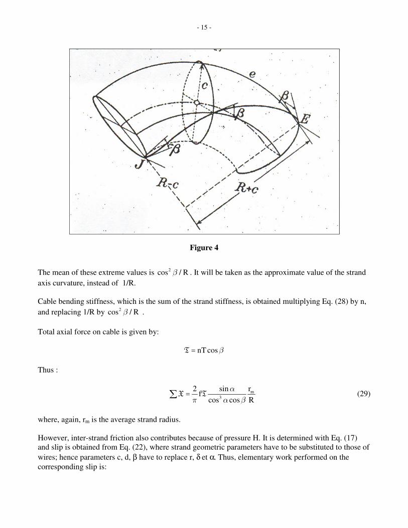
- 15 -

Figure 4

The mean of these extreme values is 2cos / Rβ . It will be taken as the approximate value of the strand

axis curvature, instead of 1/R.

Cable bending stiffness, which is the sum of the strand stiffness, is obtained multiplying Eq. (28) by n,

and replacing 1/R by 2cos / Rβ .

Total axial force on cable is given by:

nT cosβ=T

Thus :

m

3

r2 sinf

cos cos R

α

π α β=åX T (29)

where, again, rm is the average strand radius.

However, inter-strand friction also contributes because of pressure H. It is determined with Eq. (17)

and slip is obtained from Eq. (22), where strand geometric parameters have to be substituted to those of

wires; hence parameters c, d, β have to replace r, δ et α. Thus, elementary work performed on the

corresponding slip is:

- 16 -

1

c d cf H sin d

R sin cos sinϕ ϕ

β β β

This yields the average value for a given strand :

1 2

2 c sinf T

R cos

β

π β

This value, multiplied by the number of strands n has to be added to Eq. (29).

Thus, cable stiffness is given by:

( ) m 13 3

2 sin sinfr f c

R cos cos cos

α β

π α β β

æ öç ÷= +ç ÷è ø

TX (30)

Inter-strand friction coefficient f1 may be different from inter-wire coefficient f. This because of the

differing contacting surfaces, but also, it will depend on angle ψ between wires of adjacent strands,

which itself depends on the type of cable lay, parallel or cross lay (Section 2).

8. Bending tensile forces

It has been assumed that slip due to bending was a result of wire inextensibility. This hypothesis is not

sufficient to explain the actual cable behavior. It is indeed more logical to assume that, as curvature is

increased, wire tensile forces increase up to a point at which friction force reaches a limit value. At that

point, there is impending slip.

These tension increments, noted ∆t, which differ in each wire, will be called bending tensions.

In the classical solid beam theory, bending tensions are parallel to the beam axis. If beam curvature and

tension are given, these bending tensions are constant.

Thus, for a solid prismatic beam, it is only in the case of a variable curvature that internal equilibrium

requires non-zero forces parallel to beam axis between parallel layers.

In a strand, on the contrary, bending tensions are parallel to each wire axis. Even when curvature is

uniform, they vary along each wire from one point to the other. They depend on distance y from neutral

axis, which itself is a function of angle φ.

Hence, there must be a tangential force V acting on a wire surface.

It is assumed that ∆t is a force acting on a square cross-section, δ by δ, within which the round wire

section is inscribed.

In the same fashion, tangential force V is assumed to act on a band, width δ, length δ.

Hence, a given wire is acted upon by a tangential force per unit length V/δ.

- 17 -

Assuming that lateral mode of contact prevails, limit value on force V is given by:

VfN£

δ (31)

where N is given by Eq. (15) . It is a force per unit length and it corresponds to a band, width δ, as

defined for each wire.

As with slip displacements in Section 5, with uniform strand curvature, it is logical to assume that

bending tension ∆t, as well as tangential force V, take the same value for a given distance y from the

neutral axis. That is, for any wire, they will depend only on r sinϕ .

Figure 5

Consider two same-layer adjacent wires (Fig. 5). Their respective axes a and b are at a distance δ and

make an angle α with respect to strand axis. Take points A’ and B on a straight line parallel to direction

x. Bending forces ∆t on corresponding sections must take the same value.

Consider now transverse direction h, from B to A, taken, as point A’, on axis a. Bending force ∆t must

vary in the same fashion, going either from A to A’, or from A to B.

This condition yields:

( t) ( t)AA

h

∆ ∆

�

¶ ¶¢ =¶ ¶

δ (32)

where :

AA tan¢=δ α (33)

- 18 -

Besides, equilibrium of wire element d� requires that tension variation ∆t has to be balanced by the

differential on tangential force Vd /� δ acting on its side, which is:

dV dh

h

�æ ö¶ç ÷ç ÷¶ è øδ

Noting that dh = δ, such differential becomes: V

dh�

¶

¶

Thus, the equilibrium condition yields:

( t) V0

h

∆

�

¶ ¶+ =

¶ ¶ (34)

Using Eqs (32) and (33), it yields :

( t) Vtan 0

h h

∆¶ ¶+ =

¶ ¶α (35)

Thus :

t tan V cst∆ + =α

However, near the section neutral axis, ∆t = 0, and relative slip (s)1 between adjacent same layer wires

also vanishes, as seen from Eq. (22), Thus the integration constant in the above equation must vanish.

Hence:

V t tan∆= - α (36)

This implies that, on the strand cross-section, axial and tangential bending forces are proportional.

Compared to the solid beam case, this is a distinctly different behaviour.

In boundary condition Eq. (31), V is a strictly positive quantity. Force N being given by Eq. (15) and

letting:

0t t t∆= ±

limit value (∆t)0 of bending forces due to friction is:

( ) 0

0

t f tant

1 f tan∆∓ =

±

α

α (37)

In Eq. (37), the upper sign applies in the compression side, where t < t0 ; slip limit is smaller, and slip

will initiate in that region. The lower sign applies in the tension side.

9. Strain and slip

- 19 -

It is first assumed that wires behave as in a solid beam, and that the plane cross-section hypothesis is

valid. Stretch of wire element d� , on layer of radius r, is given by Eq. (20).

Corresponding strain is:

2(d ) ycos

d R

∆ �

�= =ε α (38)

Figure 6

Also, displacement in direction x of the end point A of element OA d�= is y

dxR

. Taking its

projection onto the normal direction to � and dividing by d� (Fig. 6), one gets the rotation u of

element d� :

dx(y / R)sin ysin cos

dx / cos R=α

α αα

(39)

This is of course assuming that transverse contraction of strand resulting from axial strain is neglected.

In a direction normal to wire axis, and in plane tangent to cylinder of radius r, line element dh OB=

projects onto strand axis as 1

dx dh sin= α . Displacement of point B with respect to O has a component

parallel to the x direction :

1

yBB dx

R¢ =

Projection of BB’ onto the normal direction to h, divided by dh, yields its angle of rotation and it is

equal, in absolute value and opposite direction, to Eq. (39).

Shear strain is the algebraic difference between the two rotations, and is equal to twice Eq. (38), that is

y2sin cos

R= -γ α α (40)

It is negative when y > 0, as the angle between initially orthogonal elements d and dh� is now larger

than 90°.

- 20 -

Letting a be the wire cross-section, relationship between bending forces ∆t, tangential forces V, and

corresponding strains are:

2yt Ea Ea cos

R

yV KEa 2KEa sin cos

R

∆ = =

= = -

ε α

γ α α

(41)

where K is a factor such that, when multiplied by the wire axial elastic modulus, one gets the ratio

between tangential forces and shear strain.

Combining Eqs. (40), (41) and Eq. (36) found in the preceding section from the condition of internal

equilibrium, yields

1K

2=

Correlation factor between tangential force and strain appears to be independent on strand internal

structure. According to this approach, it is obtained arbitrarily from an equivalent solid body.

10. A direct calculation of factor K

Another approach is tried, based on the following remark. Assume that tangential force per unit length

V/δ , acting parallel to wire generator g , is uniformly distributed over chord 2c, drawn at distance h

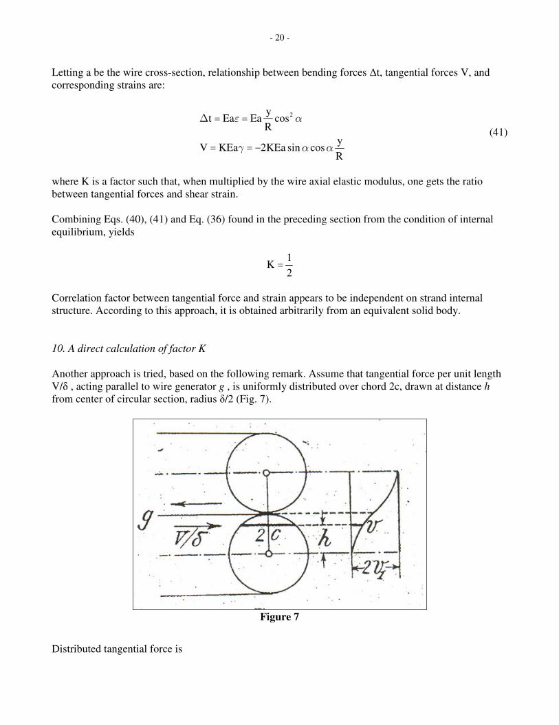
from center of circular section, radius δ/2 (Fig. 7).

Figure 7

Distributed tangential force is

- 21 -

22

V KEa

2c2 h

4

= =

-

γτ

δ δδ

It acts on the circular section chords, starting from that point at which the given wire is in contact with

adjacent wire, up to the diameter normal to the loading plane. It corresponds to warping of wire cross-

section.

Consider the radial line, belonging to the loading plane, along which distance h is measured. It

undergoes a displacement v such that, at any point:

1

2 2

2

dv E 4hK 1

dh G 4 G

-æ öç ÷= = -ç ÷è ø

τ πγ

δ

Integrating from h = 0 to h = δ/2, one gets the displacement at the contact point:

2

1

Ev K

16 G=πγ δ (42)

Relative displacement of corresponding points on same layer adjacent wires is twice this value.

Letting 12v= γ

δ, this yields

2

8 GK

E=π

(43)

Using typical values for the ratio of elastic moduli ratio, this yields a factor K of about 1/3.

Whatever the validity of this approach, as well as the interpretation that can be given to the diverging K

values of 1/2 , given by Eq. (41), and 1/3 found above, it looks obvious that the plane section

hypothesis (that a strand plane cross-section remains plane after bending), does not yield enough

parameters in order to satisfy system deformation conditions.

11. Bending forces taking into account cross-section warping

Thanks to Prof. Placido Cicala’s kind suggestion, it can be shown that a more general approach of this

problem can be obtained by dropping the plane section hypothesis. This means that a point on a wire

axis is allowed to undergo a displacement u with respect to the strand cross-section on which it is

located before bending, without loss of solidarity between wires in contact. Such displacement u is a

function of parameters φ and r only.

Function u has the same geometrical properties as slip s found in Section 5, where wires were supposed

to be inextensible; here, however, it is a displacement arising from wire elasticity.

- 22 -

Variation of element d� elastic elongation arising from displacement u is given by

ud��

¶

¶ (44)

Dividing by d� yields its value per unit length. It provides a term to be added to the expression for

strain ε found in Eq. (38):

u u u sin

r� �

¶ ¶ ¶ ¶= =

¶ ¶ ¶ ¶

ϕ α

ϕ ϕ (45)

Similarly (Fig. 5), consider a displacement in direction h, perpendicular to wire axis on a given layer.

For shear strain γ, the corresponding term to be added to the one given by Eq. (40) is

u u u 1

h h r cos

¶ ¶ ¶ ¶= =

¶ ¶ ¶ ¶

ϕ

ϕ ϕ α (46)

With y r sin= ϕ , normal and tangential bending forces are given by

2r u sint Ea cos sin

R r

u 1 rV KEa 2 sin cos sin

r cos R

∆æ ö¶ç ÷= +ç ÷¶è øæ ö¶ç ÷= -ç ÷¶è ø

αα ϕ

ϕ

α α ϕϕ α

(47)

Using Eq. (36), these equations yield :

2

2 2u r(K sin ) sin cos (2K 1)sin

R

¶+ = -

¶α α α ϕ

ϕ (48)

Integration with respect to variable φ yields :

2

2

2

ru k cos

R

sin cos (1 2K)with k

K sin

ϕ

α α

α

=

-=

+

(49)

As previously, the hypothesis according to which function u, as does function s, vanishes at the upper

and lower points of a given wire loop, has been taken into account in the integration.

Eq. (48) does not impose a specific value on parameter K. However, it leads to new equations for the

bending forces:

- 23 -

2

22

2

y yt Ea(cos k sin ) Ea with :

R R

1 2sinK cos

K sin

α α ξ

αξ α

α

∆ = - =

+=

+

(50)

If, for example : K = 1/3 and α = 17°,

It yields : k = 0.213 and ξ = 0.85

while the plane section hypothesis yields ξ = 0.914.

12. Bending tension diagram

In both cases, Eqs (41) and (50) only apply as long as tangential force is not greater than friction limit,

i.e. as long as Eq. (31) holds. Thus, they apply as long as bending tensions are smaller than limit value

(∆t)0 given by Eq. (37).

Ordinates of a wire stick and slip regions boundary points are given by:

0 01 2t ty yf tan f tan

R Ea (1 f tan ) R Ea (1 f tan )= - =

- +

α α

ξ α ξ α (51)

Letting for example f = 0.15 and Ea = 500t0 :

4 41 2y y1.15 10 1.05 10

R R

- -= ´ - = ´

yielding an average value of 1.1× 10-4

.

Outside the slip region, (∆t) keeps its constant value (∆t)0 , and its variation can be shown as in Fig. (8).

Figure 8

In Eq. (51) denominator, neglecting f tanα compared to unity, y1 and y2 absolute values, as well as

that of (∆t)0 in Eq. (37), simplify to:

- 24 -

010 0

ty tanf ( t) f tan t

R Ea∆= =

αα

ξ (52)

Thus, as strand curvature increases (or else, as radius of curvature R decreases), wire stick zone, of

amplitude 2y1 , decreases.

In practical cable machines, it is possible to consider that, at cable/pulley contact, R ≤ 50d, yielding:

1y0.0055

d£

which means that the stick zone extends above and below the neutral axis at a distance smaller than

1/100 of strand diameter d.

Thus, one may assume that (∆t)0 applies over the whole section, with a plus sign in the extension and a

minus sign in the compression region.

The absolute value of the corresponding elastic strain is:

0 0( t) f tan t

Ea Ea

∆=

α

It corresponds to a slip s’ which has to be subtracted from slip s obtained with the inextensible wire

hypothesis.

Recalling that the upper (convex side) and lower (concave side) sections of a wire undergo no

displacement, one gets:

0tan ts f

Ea�

×¢ =α

where � is a wire length measured from the closest fixed section.

Maximum value of s’ is noted S’ occurring at section neutral axis. At that point, r 2sinπ α=� (a

quarter of a wire loop). Hence:

0trS f

2cos Ea¢ =

π

α

which increases with ratio t0/Ea.

On the contrary, from Eq. (21’), maximum S of slip function s increases with ratio r/R. Taking the

usual values for f and α, both displacements may be compared:

0t rS 0.245r S 3.13r

Ea R¢ = =

- 25 -

With the selected conditions, S’ is quite small compared with S. This confirms the validity of the

inextensible wire hypothesis, used in Section 6, where only slip s was used in the friction work

computation.

13. Reacting bending moments

Reacting elastic bending moment has two components:

1. A component arising from wire bending stiffness acting independently. For a simple strand, it is

given by the equation:

2 3

1

cosM ZEa

4 R

æ öç ÷= ç ÷è ø

δ α (53)

Indeed, 2cos / Rα is the average wire curvature increase. Besides, individual wire bending moments

are vectors making an angle α with the resulting moment. It is the sum of their projections onto the

strand cross-section.

2. A component arising from bending tensions. Within the stick region, they are proportional to

distance from neutral axis. In the slip region, they have the constant value (∆t)0 .

Hence, using Eqs (50) and (52):

1

1

y y2

2 00 y

EaM 2 y 2f tan t y

R

¢

= +å åξ α (54)

where y’ is the ordinate of wire section center most distant from neutral axis.

In Eq. (54), discrete sums Σ can be replaced by integrals over the strand cross-section.

This is done by multiplying and dividing by 2 dx.dy=δ , as in the summation, each wire is replaced by

a circumscribed square.

Thus, assuming a strand compact structure:

2 2 2 2 2

2 2

1 2y y dxdy r y y dy= = -òò òåδ δ

in which the x integration has been performed over a cord of circle, radius r. Then, a second integration

must be performed: 4 2 2

2 2 2 2 2 2 2 1

2

1 r (r 2y )r y y dy y(r 2y ) r y sin

8 16 r

- -- = - - - -ò

- 26 -

At the lower boundary y=0, this expression yields 4

r

32-π

. Thus, in Eq. (54), first term becomes:

( )4 2 2

1 2 2 2 20 0 12 1 0 1 0 12 2

0

r r 2yEaM cos y r 2y r y

2R 2 r

-é ù-¢ ê ú= - - -ê úë û

ξ

δ

Letting 1 0

y r cos= λ , it yields :

4

02

Er sin 4M 2

16 R 2

é ù¢ = - +ê ú

ê úë û

ξπ λπ λ (55)

where 0

r d 2= is radius of strand circumscribed circle.

Similarly:

( )3 2

2 2 2 2 2

2 2 2

1 1 2y ydxdy r y dy r y

3= = - = - -ò òåδ δ δ

Considering the second sum boundaries, y and r become, with r = r0

( )3

3 22 2 300 12 2

2r2r y sin

3 3- = λ

δ δ

Hence, using Eq. (52) to get y1 in terms of R :

( )2 2

3 22 20 1

2 0 1 02 2

t r sin4 4M f tan r y f tan t

3 3¢¢ = - =

λα αδ δ

(56)

First term has limit value ¢W . It corresponds to the solid section hypothesis which applies up to

minimum radius of curvature R’. This can be checked from Eq. (52) and letting 0

y r= . This limit case

shall be referred to as the critical curvature.

Thus

0 0r tf tan

R ' Ea=

α

ξ

And, consequently :

3

0 0r tf tan

Ea 4 Ea

πα

δ δ

¢ æ öç ÷= ç ÷è ø

W (57)

In this case, the moment second term vanishes.

- 27 -

Beyond that point, wires are in the slip regime. When slip is complete, wires being completely

independent, bending moment reaches a limit value ¢¢W . Such limit state is an asymptotic value.

Bending moment tends towards that value as radius R decreases, indicating a decreasing strand

incremental resistance to bending.

That limit value is obtained from Eq. (56), by letting 1

y 0= . Thus:

3

0 0r t4f tan

Ea 3 Eaα

δ δ

¢¢ æ öç ÷= ç ÷è ø

W (58)

Ratio of these limit values is a constant :

0.58¢=

¢¢W

W

Finally, one should note that moment ¢¢W is in fact friction moment Mw, which was obtained in

Section 6, calculating work dissipation from wire slip. This may be checked by comparing Eqs. (28)

and (58), which can be rewritten under the form

3

0w m3 2 2

r2 sin 4 sin TM fT r f

cos 3 cos Z

α α

π α α δ¢¢= =W (59)

Using Eqs (8) and (12) for compact systems :

2 2om 0

2rr Z 3r

3= =δ

they are found to have a quite close value.

14. Moment-curvature relationship

As seen, a strand reaction bending moment is dependent on three terms. Variation of these terms has

been calculated in the following particular case: a four layer, compact structure, simple strand, made of

6 + 12 + 18 + 24 = 60 wires. Outer radius is r0 = 4.5 δ. Using typical values f = 0.15 and α = 17°, slip

starts at 4R (4.5 10 /1.1)¢ = ´ δ , and it may be considered as complete at R / 1000=δ .

Taking Ea = 500 t0 , the following table shows intermediate values.

Radius R’, which corresponds to critical bending curvature, is slightly above 40000δ. The 2

M¢ and 2

M¢¢

values appearing in the first column correspond respectively neither to ¢W nor to zero; albeit differing

little from them.

R /1000δ 40 30 20 10 1

- 28 -

1 0y / (r / ) cos=δ δ λ 4.4 3.3 2.2 1.1 0.11

11000M / Eaδ 0.08 0.11 0.16 0.33 3.28

21000M / Ea¢ δ 6.97 4.93 2.52 0.67 0

21000M / Ea¢¢ δ 0.09 3.56 7.52 10.34 11.2

1000M / Eaδ 7.14 8.60 10.20 11.34 14.48 2MR / Ea=θ δ 285.6 258 204 113.4 14.5

Second row from bottom is the sum of the three preceding rows, yielding the resulting bending moment

M, which corresponds to the strand bending resistance.

Last row is the product of that second row from bottom, by the top row, that is:

2

MR

Ea= θ

δ

θ is a factor such that aδ2θ is the strand equivalent moment of inertia for the corresponding imposed

curvature.

It should be compared to its lower and upper values. The former corresponds to the complete slip

hypothesis, where bending inertia is the sum of individual wire inertia (θ =Z/16). The latter , which

corresponds to a solid section, is obtained by adding a term 21a zr

2å . In this case, the θ factor is

increased by a term

21 r

a z2

æ öç ÷ç ÷è ø

åδ

.

With the above example numerical values, the θ lower and upper bounds are:

3.75 3.75 300¢ ¢¢= = +θ θ

θ¢¢ differs slightly from the value shown in the first column. This may result from the fact that radius R

is slightly smaller than limit radius R’. Or else, it results from the error made by substituting integrals

to finite sums in the M calculation.

θ¢ is also much smaller than the value shown in the last column. This results from the fact that the

latter takes into account the contribution of limit bending tensions ( )0t∆ arising from tangential

friction forces.

The above numerical values are shown graphically in Fig. 9. There, curves 1 2 2

M M M¢ ¢¢ as well as

resultant M are shown vs curvature 1/R.

These curves show the stages of the bending process.

- 29 -

Figure 9

At first, when radius of curvature is large, strand behaves as a solid elastic beam, wires being perfectly

bound to one another. There is a linear moment-curvature relationship (straight line AB).

When reaching critical curvature, there is impending slip and bending tension diagram (Fig. 8) shows a

slope discontinuity: the center part is still a straight line, corresponding to a linear variation with

respect to distance from neutral axis; while upper and lower parts of diagram are vertical lines,

corresponding to a constant ordinate. These constant tension regions increase as curvature increases.

During this process, the elastic bending moment may be considered as the sum of two separate

components, which correspond to both regions of the bending tension diagram: first term, 2

M¢ ,

decreases rapidly as curvature increases, while second term , 2

M¢¢ , increases rapidly. The sum increases

with curvature, though more slowly (curve BC).

In the meantime, moment component which arises from independent wire bending (the M1 term)

increases linearly with curvature 1/R. Thus, its diagram is a straight line through the origin. As

curvature increases, it becomes more important with respect to the other components. At some point,

2M¢ is practically zero while

2M¢¢ is almost constant. This explains why curve DE (drawn at a different

curvature scale in order to extend diagram) corresponds to an M curve which is almost identical to the

M1 curve.

Beyond critical curvature, slip corresponds to some energy dissipation. It is due to friction forces work

which has been found in Section 7, where X is an equivalent friction force per unit length of strand.

- 30 -

The calculation was based on the inextensible wire hypothesis, which tends to overestimate the friction

work as displacements s’ from Section 12, should be subtracted from slip s.

This friction work is the main component of the process. In fact, in most of the diagram (in the case of

Fig. 9), 9/10 of its span, corresponding to 510 / Rδ between 10 and 100), variable moment 2

M¢¢ differs

very little from its limit value ¢¢M . Recall from Eq. (59) that it is the so-called friction moment.

In the strand bending process, only a small part of the total work (the area under the curve M vs 1/R)

corresponds to the increase in the elastic potential, arising from wire axial and bending deformation.

With the elastic moment component M1 it is easily determined through the formula 1M1

2 R.

Increase of elastic potential due to M2 is the sum of deformation work from wire bending tensions, that

is:

( ) ( )22

0t dt d

2Ea 2Ea

∆∆ ��

They correspond respectively to these parts of the cross-section in which ∆t varies linearly, and in

which 0

t t cst∆ ∆= =

With dx d cos�= α , and using the corresponding ∆t value, it yields:

1

1

2 2y r2 22 2

020 y

dL dLEa f sin tany t y

dx cos R dx Ea

¢ ¢¢= =å åξ α α

α

The first summation has already been determined in the calculation of 2

M¢ . It is given by the

expression between parentheses in Eq. (55) divided by 4δ2. Hence:

2 2dL M1

dx 2 cos R

¢ ¢=

ξ

α (60)

which confirms the interpretation given for parameter ξ as a warping correction parameter.

Besides, one has the following relationship:

1

2r0

2y

ry ( sin cos )= -å λ λ λδ

Indeed, right-hand member is the area of a circular segment, radius 0

r , and central angle

1 1

0

y2 2cos

r

-æ öç ÷= ç ÷è ø

λ divided by δ2. Thus, using Eq. (56):

- 31 -

2 2dL M3

cosdx 4 R

¢¢ ¢¢= ξµ α (61)

in which parameter µ is defined as :

3

cos ( sin cos )

sin

-=

λ λ λ λµ

λ

Using the same data as in the example given at the beginning of this section, typical values of µ are

shown in the following table.

R /1000δ 40 30 20 10 1

µ 0.61 0.755 0.464 0.289 0.037

Increase of the elastic potential due to tensions (∆t)0 may thus be considered as the work contribution

from their bending moment 2

M¢¢ . Its contribution decreases rapidly as curvature increases, precisely

because energy dissipation increases correspondingly.