Embed Size (px)
Citation preview

Standard Method of Test for Determining the Flexural Creep Stiffness of Asphalt Mixtures Using the Bending Beam Rheometer (BBR) AASHTO Designation: T xxx-xx PROVIDED AS AN EXAMPLE ONLY - NOT FOR DISTRIBUTION

Standard Method of Test for Determining the Flexural Creep Stiffness of Asphalt Mixtures Using the Bending Beam Rheometer (BBR) AASHTO Designation: T xxx-xx 1. SCOPE
1.1. This test method covers the determination of the flexural creep stiffness or compliance of asphalt
mixtures by means of a bending beam rheometer. It is applicable to material having a flexural stiffness value from 2 GPa to 20 GPa (creep compliance values in the range of 0.5 nPa–1 to 0.05 nPa–1). The test apparatus is designed for testing within the temperature range from –36 to 0°C.
1.2. Test results are valid for beams of asphalt mixtures that deflect more than 15 µm and less than
150µm (550 microstrains), when tested in accordance with this method. 1.3. This standard may involve hazardous materials, operations, and equipment. This standard does
not purport to address all of the safety concerns associated with its use. It is the responsibility of the user of this procedure to establish appropriate safety and health practices and to determine the applicability of regulatory limitations prior to use.
2. REFERENCED DOCUMENTS
2.1. AASHTO Standards: AASHTO M 320, Performance-Graded Asphalt Binder AASHTO T 166, Bulk Specific Gravity of Compacted Hot-Mix Asphalt Using Saturated
Surface-Dry Specimens AASHTO T 269, Percent Air Voids in compacted Dense and Open Asphalt Mixtures AASHTO T 312, Preparing and Determining the Density of Hot Mix Asphalt (HMA)
Specimens by Means of the Superpave Gyratory Compactor AASHTO T322 Standard Method of Test for Determining the Creep Compliance and
Strength of Hot Mix Asphalt (HMA) Using the Indirect Tensile Test Device 2.2. ASTM Standards:
C 670, Practice for Preparing Precision and Bias Statements for Test Methods for Construction Materials
C 802, Conducting an Interlaboratory Test Program to Determine the Precision of Test Methods for Construction Materials
D 4123, Indirect Tension Test for Resilient Modulus of Bituminous Mixtures D 5361, Sampling Compacted Bituminous Mixtures for Laboratory Testing E 77, Standard Test Method for Inspection and Verification of Liquid-in-Glass Thermometers E 220, Method for Calibration of Thermocouples by Comparison Techniques
2.3. Deutche Industrie Norm (DIN) Standards:
43760, Platinum Resistance Thermometer

3. TERMINOLOGY 3.1. Definitions: 3.1.1. asphalt mixture—an asphalt-based composite material that consists of asphalt cement, coarse and
fine aggregates, filler, and air voids. 3.2. Descriptions of Terms Specific to This Standard: 3.2.1. flexural creep—a test in which a simply-supported asphalt mixture prismatic beam is loaded with
a constant load at its midpoint and the deflection of the beam is measured with respect to loading time.
3.2.2. flexural creep compliance, D(t)—ratio obtained by dividing the time-dependent maximum
bending strain in the beam by the time-independent maximum bending stress.
3.2.3. measured flexural creep stiffness, Sm(t)—ratio obtained by dividing the maximum bending stress in the beam by the maximum bending strain. S(t) is the inverse of D(t). S(t) has been used historically in asphalt technology while D(t) is commonly used in studies of viscoelasticity.
3.2.4. estimated flexural creep stiffness, S(t)—the creep stiffness obtained by fitting a second order
polynomial to the logarithm of the measured stiffness, from 8.0 to 1000 seconds, as a function of the logarithm of time.
3.2.5. m-value—absolute value of the slope of the logarithm of the estimated stiffness curves versus the
logarithm of the time. Note that m-value estimation for any time during the test is based on the creep test results for the entire duration of the test.
3.2.6. contact load—load required to maintain positive contact between the beam and the loading shaft,
and equal to 35 ±10 mN. 3.2.7. seating load—load of 1-s duration required to seat the beam, and equal to 4000 ±100 mN. 3.2.8. test load—load of 1000-s duration required to determine the stiffness of the material being tested,
and equal to 4000 ±100 mN. 3.2.9. testing zero time, s—time at which the signal is sent to the solenoid valve to switch from zero load
regulator (contact load) to the testing load regulator (test load).
4. SUMMARY OF TEST METHOD 4.1. The bending beam rheometer measures the mid-point deflection of a simply supported beam of
asphalt mixtures subjected to a constant load applied to the mid-point of the beam. The device operates only in the loading mode; recovery measurements are not obtained.
4.2. A test beam is placed in the controlled temperature fluid bath and loaded with a constant load for
240-s. The test load (4000 ±100 mN) and the midpoint of deflection of the beam are monitored versus time using a computerized data acquisition system.

4.3. The maximum bending stress at the midpoint of the beam is calculated from the dimensions of the beam, the span length, and the load applied to the beam. The maximum bending strain in the beam is calculated for the same loading times from the dimensions of the beam and the deflection of the beam. The stiffness of the beam is calculated by dividing the maximum stress by the maximum strain.
4.4. The load and deflection at 0.0 and 0.5 s are reported to verify that the full-testing load (4000
±100 mN) during the test is applied within the first 0.5 s. They are not used in the calculation of stiffness and m-value and should not be considered to represent material properties. The rise time of the load (time to apply full load) can be affected by improper operation of the pressure regulators, improper air bearing pressure, malfunctioning air bearing (friction), and other factors. By reporting the 0.0 and the 0.5 s signals, the user of the test results can determine the conditions of the loading.
5. SIGNIFICANCE AND USE 5.1. The test temperature for this test is related to the temperature experienced by the pavement in the
geographical area for which the asphalt binder is intended. 5.2. The flexural creep stiffness or flexural creep compliance, determined from this test, describes the
low-temperature, stress-strain-time response of asphalt mixtures at the test temperature within the linear viscoelastic response range.
5.3. The low-temperature thermal cracking performance of paving mixtures is related to the creep
stiffness and the slope of the logarithm of the creep stiffness versus the logarithm of the time curve of the asphalt mixture.
5.4. The creep compliance is used in the low temperature algorithm of the AASHTO Mechanistic
Empirical Pavement Design Guide to calculate thermal stresses used in predicting pavement performance.
6. APPARATUS 6.1. Bending Beam Rheometer (BBR) Test System—A bending beam rheometer (BBR) test system
consisting of (1) a loading frame which permits the test beam, supports, and the lower part of the test frame to be submerged in a constant temperature fluid bath, (2) a controlled temperature liquid bath which maintains the test beam at the test temperature, and (3) a computer-controlled automated data acquisition component, (4) specimen molds, and (5) items needed to calibrate and/or verify the BBR.
Note 1—The buoyant force in the liquid of the bath provides partial counterbalance of the weight of the mixture beam. The remainder of the weight is approximately equal to 90 mN, which can be neglected for a testing load of 4000 mN.
6.1.1. Loading Frame—A frame consisting of a set of sample supports, a blunt-nosed shaft that applies
the load to the midpoint of the test specimen, a load cell mounted on the loading shaft, a means for zeroing the load on the test specimen, a means for applying a constant load to the loading shaft, and a deflection measuring transducer attached to the loading shaft. A schematic of the device is shown in Figure 1.

Figure 1—Schematic of the Bending Beam Rheometer 6.1.1.1. Loading System—A loading system that is capable of applying a contact load of 35 ± 10 mN to
the test specimen and maintaining a test load of 4000 ±100 mN. 6.1.1.2. Loading System Requirements—The rise time for the test load shall be less than 0.5 s. The rise
time is the time required for the load to rise from the 35 ±10 mN contact load to the 4000 ±100 mN test load. During the rise time, the system shall dampen the test load to 4000 ±100 mN. Between 0.5 and 5.0 s, the test load shall be within ±100 mN of the average test load, and thereafter shall be within ±50 mN of the average test load.
6.1.1.3. Sample Supports—Sample supports with specimen support strips 3.0 ±0.30 mm in top radius and
inclined at an angle of 45 degrees with the horizontal (see Figure 1). The supports, made of stainless steel (or other corrosion resistant metal), are spaced 102.0 ±1.0 mm apart. The width of the supporting area of the supporting strips shall be 9.5 ±0.25 mm. This is required to ensure that the edges of the specimen, resulting from the molding procedure, do not interfere with the mid-span deflection of the specimen measured during testing. The supports shall also include vertical alignment pins 2 to 4 mm in diameter placed at the back of each sample supports at 6.75 ±0.25 mm from the center of the supports. These pins should be placed on the back side of the support to align the specimen on the center of the supports. See Figure 1 for details.
6.1.1.4. Loading Shaft—A blunt-nosed loading shaft (with a spherical contact point 6.25 (±0.30) mm in
radius) continuous with a load cell and a deflection measuring transducer which is capable of

applying a contact load of 35 ±10 mN and maintaining a test load of 4000 ±100 mN. The rise time for the test load shall be less than 0.5 s where the rise time is the time required for the load to rise from the 35 ±10 mN preload to the 4000 ±100 mN test load. During the rise time the system shall dampen the test load after the first five seconds to a constant ±50 mN value.
6.1.1.5. Load Cell—A load cell with a minimum capacity of 9,806 mN and having a minimum resolution
of 2.5 mN mounted in-line with the loading shaft and above the fluid to measure the contact load and the test load.
6.1.1.6. Linear Variable Differential Transducer (LVDT)—A linear variable differential transducer or
other suitable mounted device mounted axially above the loading shaft capable of resolving a linear movement ≤0.15 µm with a range of at least 6 mm to measure the deflection of the test beam.
6.1.2. Controlled-Temperature Fluid Bath—A controlled temperature liquid bath capable of maintaining
the temperature at all points within the bath between –36 and 0°C within ±0.1°C. Placing a cold specimen in the bath may cause the bath temperature to fluctuate ±0.2°C from the target test temperature; consequently, bath fluctuations of 0.2°C during isothermal conditioning shall be allowed.
6.1.2.1. Bath Agitator—A bath agitator for maintaining the required temperature homogeneity with
agitator intensity such that the fluid current does not disturb the testing process and mechanical noise caused by vibrations is less than the resolution specified in Sections 6.1.3 and 6.1.3.1.
6.1.2.2. Circulating Bath (Optional)—A circulating bath unit separate from the test frame which pumps
the bath fluid through the test bath. If used, vibrations from the circulating system shall be isolated from the bath test chamber so that mechanical noise is less than the resolution specified in Sections 6.1.3 and 6.1.3.1.
6.1.3. Data Acquisition System—A data acquisition system that resolves loads to the nearest 2.5 mN,
beam deflection to the nearest 0.15 µm, and bath fluid temperature to the nearest 0.1°C. The system shall sense the point in time when the signal is sent to the solenoid valve(s) to switch from zero load regulator (contact load) to the testing load regulator (test load). This is zero time. Using this time as a reference, the system shall provide a record of load and deflection measurements relative to this time. The system shall record the load and deflection at the loading times of 0.0, 0.5, 8.0, 15.0, 30.0, 60.0, 120.0, and 240s. All readings shall be an average of three or more points within ±0.2 seconds from the loading time, e.g., for a loading time of 7.8, 7.9, 8.0, 8.1, and 8.2 seconds.
6.1.3.1. Signal Filtering—Digital or analog smoothing of the load and the deflection data may be
required to eliminate electronic noise that could otherwise affect the ability of the second order polynomial to fit the data with sufficient accuracy to provide a reliable estimate of m-value. The load and deflection signals may be filtered with a low pass analog or digital filter that removes signals of greater than 4 Hz frequency. The averaging shall be over a time period less or equal to ±0.2 s of the reporting time.
6.2. Temperature Measuring Equipment—A calibrated temperature transducer capable of measuring the temperature to 0.1°C over the range of –36 to 0°C mounted within 50 mm of the midpoint of the test specimen supports.
Note 2—Required temperature measurement can be accomplished with an appropriately calibrated platinum resistance thermometer (RTD) or a thermistor. Calibrations of an RTD or thermistor can be verified as per Section 6.6. An RTD meeting DIN Standard 43760 (Class A) is recommended for this purpose. The required precision and accuracy cannot be obtained unless each RTD is calibrated as a system with its respective meter or electronic circuitry.

6.3. Items for Calibration or Verification—The following items are required to verify and calibrate
the BBR. 6.3.1. Stainless Steel (Thick) Beam for Compliance Measurement and Load Cell Calibration—One
stainless steel beam, 6.4 ±0.1 mm thick by 12.7 0.25 mm wide by 127 ±5 mm long, for measuring system compliance and calibrating the load cell.
6.3.2. Stainless Steel (Thin) Beam for Overall System Check—One stainless steel beam, 1.3 ± 0.3 mm
thick by 12.7 ±0.1 mm wide by 127 ±5 mm long, with an elastic modulus reported to three significant figures by the manufacturer. The manufacturer shall measure and report the thickness of this beam to the nearest 0.01 mm and the width to the nearest 0.05 mm. The dimensions of the beam shall be used to calculate the modulus of the beam during the overall system check. See Section 10.1.2.1.
6.4. Standard Masses—One or more standard masses are required as follows: 6.4.1. Verification of Load Cell Calibration—One or more masses totaling 100 ±0.2 g and two masses
of 2 ±0.2 g each (see Note 3) for verifying the calibration of the load cell.
Note 3—A coin may be used if the mass is confirmed to be 2 ± 0.2 g. 6.4.2. Calibration of Load Cell—Four masses, each of known mass ±0.2 g, and equally spaced in
mass over the range of the load cell. 6.4.3. Daily Overall System Check—Two or more masses, each of known mass to 0.2 g, for conducting
overall system check as specified by the manufacturer. 6.4.4. Accuracy of Masses—Accuracy of the masses in Section 6.5 shall be verified at least once each
every three years.
6.5. Calibrated Thermometers—Calibrated liquid-in-glass thermometers for verification of the temperature transducer of suitable range with subdivisions of 0.1°C. These thermometers shall be partial immersion thermometers with an ice point and shall be calibrated in accordance with Test Method E 77 at least once per year. A suitable thermometer is designated 133C. An electronic thermometer of equal accuracy and resolution may be used.
6.6. Thickness Gauge—A stepped thickness gauge for verifying the calibrations of displacement
transducer as described in Figure 3. 7. MATERIALS 7.1. Bath Fluid—A bath fluid that is not absorbed by or does not affect the properties of the asphalt
mixture tested. The mass density of the fluid bath shall not exceed 1.05 kg/m3 at testing temperatures. The bath fluid shall be optically clear at all testing temperatures.. Silicone fluids or mixtures containing silicones shall not be used.
Note 4— Suitable bath fluids include ethanol, methanol, and glycol-methanol mixtures (e.g., 60 percent glycol, 15 percent methanol, 25 percent water).

8. HAZARDS 8.1. Observe standard laboratory safety procedures when handling hot asphalt binder and preparing
test specimens. 8.2. Alcohol baths are flammable and toxic. Locate the controlled temperature bath in a well ventilated
area away from sources of ignition. Avoid breathing alcohol vapors, and contact of the bath fluid with the skin.
8.3. Contact between the bath fluid and skin at the lower temperatures used in this test method can
cause frostbite.
9. PREPARATION OF APPARATUS 9.1. Clean the supports, loading head and bath fluid of any particulates and coatings as necessary.
Note 5—Because of the brittleness of asphalt mixtures at the specified test temperatures, small fragments of asphalt mixtures can be introduced into the bath fluid. If these fragments are present on the supports or the loading head, the measured deflection will be affected. The small fragments, because of their small size, will deform under load and add an apparent deflection of the beam. Filtration of the bath fluid will aid in preserving the required cleanliness.
9.2. Select the test temperature and adjust the bath fluid to the selected temperature. Wait until the temperature stabilizes and then allow the bath to equilibrate to the test temperature ±0.1°C prior to conducting a test.
9.3. Activate the data acquisition system and load the software as explained in the manufacturer’s
manual for the test system.

Figure 2—Typical Thickness Gauge Used to Calibrate Deflection Detector

10. STANDARDIZATION 10.1. Verify the calibration of the displacement transducer, load cell, and temperature transducer as
described in Sections 10.1.1 through 10.1.6. As a minimum, each of the verification steps and their frequency of performance shall be performed as described in this section. Additional verification steps may be performed at the recommendation of the manufacturer. Calibration procedures are described in the Annex. At the option of the manufacturer, the verification and calibration steps may be combined.
10.1.1. Verification of Temperature Transducer—On each day, before conducting tests, and whenever
the test temperature is changed, verify calibration of the temperature detector by using a calibrated thermometer as described in Section 6.5. With the loading frame placed in the liquid bath, immerse the thermometer in the liquid bath close to the temperature transducer, and compare the temperature indicated by the thermometer to the temperature displayed by the data acquisition system. If the temperature indicated by the data acquisition system does not agree with the thermometer within ± 0.1°C, calibration is required.
10.1.2. Verification of Freely Operating Air Bearing—On each day, before conducting tests, verify that
the air bearing is operating freely and is free of friction. Sections 10.1.2.1 and 10.1.2.2 shall be used to verify that the shaft is free of friction. If the requirements of Sections 10.1.2.1 and 10.1.2.2 are not satisfied, friction is present in the air bearing. Clean the shaft, and adjust the clearance of the displacement transducer as per the manufacturer’s instructions. If this does not eliminate the friction, discontinue use of the BBR, and consult the manufacturer.
Note 6—Friction may be caused by a poorly adjusted displacement transducer core that rubs against its housing, an accumulation of asphalt binder on the loading shaft, by oil or other particulates in the air supply, and other causes.
10.1.2.1. Place the thin steel beam (Section 6.3.2) on the sample supports, and apply a 35 ±10 mN load to
the beam using the zero load regulator. Observe the reading of the LVDT as indicated by the data acquisition system. Gently grasp the shaft, and lift it upwards approximately 5 mm by observing the reading of the LVDT. When the shaft is released, it shall immediately float downward and make contact with the beam.
10.1.2.2. Remove any beams from the supports. Use the zero load regulator to adjust the loading shaft so
that it is free floating at the approximate midpoint of its vertical travel. Gently add a 2 g mass to the loading shelf. The shaft shall slowly drop downward under the mass.
10.1.3. Verification of Displacement Transducer—On each day, before conducting tests, verify the
calibration of the displacement transducer using a stepped gauge block of known dimensions similar to the one shown in Figure 2. With the loading frame mounted in the bath at the test temperature, remove all beams from the supports, and place the gauge block on a reference platform underneath the loading shaft according to the instructions supplied by the instrument manufacturer. Apply a 100 g ± 0.2 g mass to the loading shaft, and measure the rise of the steps with the displacement transducer. Compare the measured values as indicated by the data acquisition system with the known dimensions of the gauge. If the known dimensions as
determined from the gauge block and the dimensions indicated by the data acquisition system differ by more than ±5 µm, calibration is required. Perform the calibration, and repeat Section 10.1.1. If the requirements of Section 10.1.1 cannot be met after calibration, discontinue use of the device, and consult the manufacturer.
10.1.4. Daily Overall System Check—On each day, before conducting tests and with the loading frame
mounted in the bath, perform a check on the overall operation of the system. Place the 1.3 ±0.3

mm thick stainless steel (thin) beam of known modulus as described in Section Section 6.3.2on the sample supports. Following the instructions supplied by the manufacturer, place the beam on the supports and apply a 50.0 or 100.0 ±0.2 g initial mass (491 or 981 mN ±2 mN) to the beam to ensure that the beam is seated and in full contact with the supports. Following the manufacturer’s instructions, apply a second additional load of 100.0 to 300.0±0.2 g to the beam. The software provided by the manufacturer shall use the change in load and associated change in deflection to calculate the modulus of the beam to three significant figures. The modulus reported by the software shall be within 10 percent of the modulus reported by the manufacturer of the beam; otherwise, the overall operation of the BBR shall be considered suspect and the manufacturer shall be consulted
10.1.5. Verification of Load Cell—Verify the calibration of the load cell as follows: 10.1.5.1. Contact Load—On each day, verify the calibration of the load cell in the range of the contact
load. Place the 6.3 mm thick stainless steel compliance beam (Section 6.3.1) on the supports. Apply a 20 ±10 mN load to the beam using the zero load pressure regulator. Add the 2.0±0.2g mass as specified in Section 6.5.1 to the loading platform. The increase in the load displayed by the data acquisition system shall be 20 ±5 mN. Add a second 2.0 ± 0.2 g mass to the loading platform. The increase in the load displayed by the data acquisition system shall be 20 ±5 mN. If the increases in displayed load are not 20 ±5 mN, calibration is required. Perform the calibration. If the requirements of Section 10.1.3.1 cannot be met after calibration, discontinue use of the device, and consult the manufacturer.
10.1.5.2. Test Load—On each day, before conducting tests, verify the calibration of the load cell in the
range of the test load. Place the 6.3 mm thick stainless steel compliance beam (Section 6.4.1) on the supports. Use the zero load regulator (contact load) to apply a 20 ±10 mN load to the beam. Add the 100 g mass to the loading platform. The increase in the load displayed by the data acquisition system shall be 981 ±5 mN. Otherwise, calibrate the load cell. If the requirements of Section 10.1.3.2 cannot be met after calibration, discontinue use of the device, and consult the manufacturer.
10.1.6. Verification of Front-to-Back Alignment of Loading Shaft—Every six months, check the
alignment of the loading shaft with the center of the sample supports with an alignment gauge supplied by the manufacturer or by measurement as follows: Cut a strip of white paper about 25 mm in length and slightly narrower than the width of the compliance beam. Stick the paper strip to the center of the compliance beam with tape. Move the frame out of the bath, place the compliance beam on the supports, and place a small section of carbon paper over the paper. With the air pressure applied to the air bearing, push the shaft downward causing the carbon paper to make an imprint on the white paper. Remove the beam, and measure the distance from the center of the imprint to each edge of the beam with a pair of vernier calipers. The difference between the two measurements shall be 1.0 mm or less. If this requirement is not met, contact the manufacturer of the device.
11. PREPARATION OF TEST SPECIMENS 11.1. Tall Gyratory Cylinder (170 ±2 mm height by 150 mm diameter) - Asphalt mixture BBR beams
are obtained from gyratory compacted specimens (11.2. and 11.3.) and from field cores (11.4.). See AASHTO T 312-09 for the preparation of cylindrical gyratory mixtures specimen.
11.1. 1 This method is used when other tests, such as IDT (AASHTO R 322-07) are performed and a comprehensive direct comparison of the BBR and IDT results is needed.

11.1.2. Step 1 - The top 15 mm and the bottom 15 mm of the gyratory specimen are removed using a typical laboratory saw for mixture specimen preparation to obtain smooth surfaces. The remaining cylinder is cut into three 40 mm-thick IDT specimens, which may be tested at three different temperatures (each at one temperature) to determine the mixture creep compliance (Figure 3).
11.1.3. Step 2 - One day after IDT creep testing is completed (if performed), the specimens are further cut to obtain BBR thin beams. First, a thin slice, approximately 5 mm thick, is cut from one face of the IDT specimen to ensure a smooth surface and to remove any glue remaining from IDT buttons. Next, a 12.5 mm thick slice is cut from the remaining part of the IDT specimen, see Figure 4. This slice is used in the next two steps to prepare the BBR beams. Note that the remaining 17-18 mm part at the bottom of the IDT specimen is necessary to hold the IDT specimen during saw cutting (see Figure 4) to remove the first thin layer and then accurately cut the next slice used for the BBR beams.
11.1.4. Step 3 - The 12.5 mm thick slice is further cut from three sides to obtain 122 mm wide irregular slice, as shown in Figure 5.
11.1.5. Step 4. The slice obtained in step 3 is further cut into approximately 11 beams depending on the saw blade thickness, as shown in Figure 6. Each beam should have a size of 6.35 ± 0.05-mm thick by 12.70 ±0.05-mm wide by 127 ±2.0-mm long. Thickness and width of each beam should be measured in three points by mean of a caliper and the average reported and input in the software of the machine. A simple tile saw can be used to produce BBR mixture beams with uniform dimension. The blade has to present a continuous rim. The direction used to cut the thin beams with respect to the IDT specimens loading direction is not significant.
11.2. Normal Gyratory Cylinder (115 ±5 mm height by 150 mm diameter) 11.2.1. If IDT samples are required, then step 11.1.2. is modified as follows: the top 10 mm and the
bottom 10 mm of the gyratory specimen are removed and the remaining cylinder is cut into two 40 mm-thick IDT specimens. The remaining steps do not change.
11.2.2. If other mechanical tests are not required, then step 11.1.2. is modified as follows: the top 45 mm of the gyratory is removed and a 12.5 mm thick slice is cut from the remaining cylinder; this slice represents the middle portion of the original gyratory specimen. The remaining steps do not change.
11.3. Field Cores - The cores should be cut into slices following the procedure previously described 11.1. and 11.2., taken into consideration that typical lift thickness is 50.8 mm (2 in.) Particular attention should be given to the core surface; for very rough surfaces, the top 5 mm may have to be removed; for reasonable smooth surfaces, the top can be kept since it represents the most aged portion of the asphalt pavement
12. PROCEDURE 12.1. Two test temperature levels can be used for testing with the following loads respectively:
1961 mN at high temperature level = low temperature grade of binder + 10˚C + 12˚C, and 4413 mN at intermediate temperature level = low temperature grade of binder + 10˚C. For the low temperature level = low temperature grade of binder + 10˚C - 12˚C, it is recommended to predict the stiffness curve by applying time-temperature superposition principle to the experimental data at the intermediate and high temperature levels.

Figure 3— Cutting BBR mixture beams: Step 1
Figure 4— Cutting BBR mixture beams: Step 2
Figure 5— Cutting BBR mixture beams: Step 3
Figure 6— BBR mixture beams: Step 4

12.1.1. Place the test specimen in the testing bath and condition it at the testing temperature for 60 ±5 minutes.
Note 7—Asphalt binders may harden rapidly when held at low temperatures. This effect, which is called physical hardening, is reversible when the asphalt binder is heated to room temperature or slightly above. Because of physical hardening, conditioning time must be carefully controlled if repeatable results are to be obtained.
12.2. Checking Contact Load and Test Load—Check the adjustment of the contact load and test load
prior to testing each set of test specimens. The 6.35-mm thick stainless steel beam shall be used for checking the contact load and test load.
Note 8—Do not perform these checks with the thin steel beam or an asphalt test specimen.
12.2.1. Place the thick steel beam in position on the beam supports. Using the test load regulator valve,
gently increase the force on the beam to 1961 ±50 mN or 4413 ±50 mN test load. 12.2.2. Switch from the test load to the contact load, and adjust the force on the beam to 35 ± 10 mN.
Switch between the test load and contact load four times. 12.2.3. When switching between the test load and contact load, watch the loading shaft and platform for
visible vertical movement. The loading shaft shall maintain contact with the steel beam when switching between the contact load and test load while maintaining these loads at 35 ± 10 mN and 1961 ±50 mN or 4413 ±50 mN test load, respectively.
12.2.4. Corrective Action—If the requirements of Sections 12.2.1 to 12.2.3 are not met, the device may
require calibration as per the manufacturer’s instructions or the loading shaft may be dirty or require alignment (see Section 10.1.2). If the requirements of Sections 12.2.1 to 12.2.3 cannot be met after calibration, cleaning, or other corrective action, discontinue use of the device and consult the equipment manufacturer.
12.3. Enter the specimen identification information, test load, test temperature, time the specimen is
placed in the bath at the test temperature, and other information as appropriate into the computer which controls the test system.
12.4. After conditioning, place the test beam on the test supports, and initiate the loading sequence of
the test. Maintain the bath at the test temperature ±0.1°C during testing; otherwise, the test shall be rejected.
12.5. Manually apply a 35 ± 10 mN contact load to the beam to ensure contact between the beam and
the loading head for no more than 10 s. The specified contact load is required to ensure continuous contact between the loading shaft and support, and the specimen. Failure to establish continuous contact within the required load range gives misleading results. The contact load shall be applied by gently increasing the load to 35 ± 10 mN. While applying the contact load, the load on the beam shall not exceed 45 mN, and the time to apply and adjust the contact load shall be no greater than 10 s.
12.6. Activate the automatic test system that is programmed to proceed as follows: 12.6.1. Immediately after the application of the 35 mN contact load, increase the load from 35 ± 10 mN
to the 1961 ±50 mN or 4413 ±50 mN seating load for 1.0 ±0.1 s for high and for intermediate and low temperature levels respectively seating load for 1.0 ±0.1 s.
Note 9—The seating loads described in Sections 12.6.1 and 12.6.2 are applied and removed

automatically by the computer-controlled loading system and are transparent to the operator. Data are not recorded during the initial loading.
12.6.2. Reduce the load to 35 ±10 mN and allow the beam to recover for 20.0 ±0.1 s. 12.6.3. Apply a test load ranging as specified in Section 6.1.1.2.
Note 10—The actual load on the beam as measured by the load cell is used in calculating the stress in the beam. The initial seating and test load includes the 35 ±10 mN preload.
Note 11—Modifications of the BBR software by the manufacturer increased the resolution of deflection measurements; the latest hardware and software can resolve deflections of 0.15 microns with an accuracy of less than 1 micron
12.6.4. Remove the test load and terminate the test. 12.6.5. At the end of the initial seating load, and at the end of the test, monitor the computer screen to
verify that the load on the beam returns to 35 ±10 mN in each case. If the beam does not return to 35 ±10 mN, the test is invalid and the rheometer should be calibrated.
12.7. Remove the specimen from the supports and proceed to the next test. 13. CALCULATION AND INTERPRETATION OF RESULTS 13.1. See Annex. 14. REPORT 14.1. Report data as shown in Figure 4 that describes individual test, including: 14.1.1. Maximum and minimum temperature of the test bath measured during the 240 seconds of testing
measured at 1.0 second interval to the nearest 0.1°C, 14.1.2. Date and time when test load is applied, 14.1.3. File name of test data, 14.1.4. Name of operator, 14.1.5. Sample identification number,

Figure 4—Typical Test Report 14.1.6. Time beam in bath, 14.1.7. Time test started, 14.1.8. Any flags issued by software during test, 14.1.9. Correlation coefficient, R2
for log stiffness versus log time, expressed to nearest 0.000001, 14.1.10. Anecdotal comments (maximum 256 characters), 14.1.11. Report constants A, B, and C to three significant figures, 14.1.12. Difference between measured and estimated stiffness calculated as:
(Estimated – Measured) ×100 percent/Measured. 14.2. Report load and deflection as for times 0.0 and 0.5 seconds. 14.3. Report data as shown in Figure 4 for time intervals of 8.0, 15.0, 30.0, 60.0, 120.0, and 240 seconds
including: 14.3.1. Loading time, nearest 0.1 second;
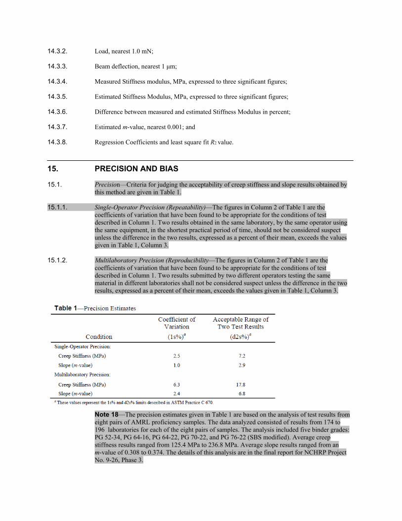
14.3.2. Load, nearest 1.0 mN; 14.3.3. Beam deflection, nearest 1 µm; 14.3.4. Measured Stiffness modulus, MPa, expressed to three significant figures; 14.3.5. Estimated Stiffness Modulus, MPa, expressed to three significant figures; 14.3.6. Difference between measured and estimated Stiffness Modulus in percent; 14.3.7. Estimated m-value, nearest 0.001; and 14.3.8. Regression Coefficients and least square fit R2 value. 15. PRECISION AND BIAS 15.1. Precision—Criteria for judging the acceptability of creep stiffness and slope results obtained by
this method are given in Table 1. 15.1.1. Single-Operator Precision (Repeatability)—The figures in Column 2 of Table 1 are the
coefficients of variation that have been found to be appropriate for the conditions of test described in Column 1. Two results obtained in the same laboratory, by the same operator using the same equipment, in the shortest practical period of time, should not be considered suspect unless the difference in the two results, expressed as a percent of their mean, exceeds the values given in Table 1, Column 3.
15.1.2. Multilaboratory Precision (Reproducibility—The figures in Column 2 of Table 1 are the
coefficients of variation that have been found to be appropriate for the conditions of test described in Column 1. Two results submitted by two different operators testing the same material in different laboratories shall not be considered suspect unless the difference in the two results, expressed as a percent of their mean, exceeds the values given in Table 1, Column 3.
Note 18—The precision estimates given in Table 1 are based on the analysis of test results from eight pairs of AMRL proficiency samples. The data analyzed consisted of results from 174 to 196 laboratories for each of the eight pairs of samples. The analysis included five binder grades: PG 52-34, PG 64-16, PG 64-22, PG 70-22, and PG 76-22 (SBS modified). Average creep stiffness results ranged from 125.4 MPa to 236.8 MPa. Average slope results ranged from an m-value of 0.308 to 0.374. The details of this analysis are in the final report for NCHRP Project No. 9-26, Phase 3.

Note 19—As an example, two tests conducted on the same material yield creep stiffness results of 190.3 MPa and 200.7 MPa, respectively. The average of these two measurements is 195.5 MPa. The acceptable range of results is then 7.2 percent of 195.5 MPa or 14.1 MPa. As the difference between 190.3 MPa and 200.7 MPa is less than 14.1 MPa, the results are within the acceptable range.
15.2. Bias—No information can be presented on the bias of the procedure because no material having
an accepted reference value is available. 16. KEYWORDS 16.1. Flexural; creep stiffness; flexural creep compliance; bending beam rheometer. ANNEX
(Mandatory Information)
A1.1 Calibration of Displacement Transducer—Calibrate the displacement transducer using a stepped
gauge block of known dimensions similar to the one shown in Figure 3. With the loading frame mounted in the bath at the test temperature, remove all beams from the supports, and place the stepped gauge block on a reference platform underneath the loading shaft according to the instructions supplied by the instrument manufacturer. Apply a 100-g mass on the loading shaft, and follow the manufacturer’s instructions to obtain a displacement transducer reading on each step. The software provided by the manufacturer shall convert the measurements to a calibration constant in terms of µm/bit to three significant figures and shall automatically enter the new constant into the software. The calibration constant should be repeatable within 10 percent from one calibration to another; otherwise, the operation of the system may be suspect.
A1.2 Calibration of Load Cell—Calibrate the load cell in accordance with the manufacturer’s
instructions using a minimum of four masses evenly distributed over the range of the load cell. The software provided by the manufacturer shall convert the measurements to a calibration constant in terms of mN/bit to three significant figures and shall automatically enter the new constant into the software. The calibration constants should be repeatable within 10 percent from one calibration to another; otherwise, the operation of the system may be suspect. Repeat the process for each test temperature.
A1.3 Calibration of Temperature Transducer—Calibrate the temperature detector by using a
calibrated thermometer of suitable range meeting the requirements of Section 10.1.5. Immerse the thermometer in the liquid bath close to the thermal detector, and compare the temperature indicated by the calibrated thermometer to the detector signal being displayed. If the temperature indicated by the thermal detector does not agree with the thermometer within ±0.1°C, follow the manufacturer’s instructions for correcting the displayed temperature to agree with the thermometer temperature.
A1.4 Determine the System Compliance—Determine the system compliance in accordance with the
manufacturer’s instructions using a minimum of four masses evenly distributed over the range of the load cell. The data acquisition software shall measure the position of the displacement transducer at each load. The compliance shall be calculated as the measured deflection per unit load. The software provided by the manufacturer shall convert the measurements to a compliance in terms of µm/N to three significant figures and shall automatically enter the compliance into the software. The compliance measurement may be performed as part of the

load cell calibration or as a separate operation. The compliance measurement shall be performed each time the load cell is calibrated. The compliance value should be repeatable within 10 percent from one determination to another; otherwise, the operation of the system may be suspect. Repeat the process for each test temperature.
A1.5 Typical Test Result—A typical test result is shown in Figure 4. Disregard measurements
obtained and the curves projected on the computer screen during the initial eight seconds of the application of the test load. Data from a creep test obtained immediately after the application of the test load may not be valid because of dynamic loading effects and the finite rise time. Use only the data obtained between 8 and 240s loading time for calculating S(t) and m.
A1.6 Deflection of an Elastic Beam—Using the elementary bending theory, the mid-span deflection of
an elastic prismatic beam of constant cross-section loaded in three-point loading can be obtained by applying Equations A1.1 and A1.2 as follows:
δ = PL3/48EI (A1.1) where: δ = deflection of beam at midspan, mm; P = load applied, N; L = span length, mm; E = modulus of elasticity, MPa; and I = moment of inertia, mm4. and: I = bh3/12 (A1.2) where: I = moment of inertia of cross-section of test beam, mm4; b = width of beam, mm; and h = thickness of beam, mm. Note A1—The test specimen has a span to depth ratio of 16:1 and the contribution of shear to deflection of the beam can be neglected.
A1.7 Elastic Flexural Modulus—According to elastic theory, calculate the flexural modulus of a
prismatic beam of constant cross-section loaded at its midspan using the following equation: E = PL3/4bh3δ (A1.3) where: E = time-dependent flexural creep stiffness, MPa; P = constant load, N; L = span length, mm; b = width of beam, mm; h = thickness of beam, mm; and δ = deflection of beam, mm.
A1.8 Maximum Bending Stress—The maximum bending stress in the beam occurs at the midspan at
the top and bottom of the beam. Calculate σ thus: σ = 3PL/2bh2
(A1.4) where: σ = maximum bending stress in beam, MPa; P = constant load, N; L = span length, mm;

b = width of beam, mm; and h = thickness of beam, mm.
A1.9 Maximum Bending Strain—The maximum bending strain in the beam occurs at the midspan at
the top and bottom of the beam. Calculate Є using the following equation: Є = 6δh/L2
mm/mm (A1.5) where: Є = maximum bending strain in beam, mm/mm; δ = deflection of beam, mm; h = thickness of beam, mm; and L = span length, mm.
A1.10 Linear Viscoelastic Stiffness Modulus—According to the elastic-viscoelastic correspondence
principle, it can be assumed that if a linear viscoelastic beam is subjected to a constant load applied at t = 0 and held constant, the stress distribution is the same as that in a linear elastic beam under the same load. Further, the strains and displacements depend on time and are derived from those of the elastic case by replacing E with 1/D(t). Since 1/D(t) is equivalent to S(t), rearranging the elastic solution results in the following relationship for the stiffness:
S(t) = PL3/4bh3δ(t) (A1.6) where: S(t) = time-dependent flexural creep stiffness, MPa; P = constant load, N; L = span length, mm; b = width of beam, mm; h = thickness of beam, mm; δ(t) = deflection of beam, mm; and δ(t) and S(t) indicate that the deflection and stiffness, respectively, are functions of time.
A1.11 Presentation of Data: A1.11.1 Plot the response of the test beam to the creep loading as the logarithm of stiffness with respect
to the logarithm of loading time. A typical representation of test data is shown in Figure 4. Over the limited testing time from 8 to 240 seconds, the plotted data shown in Figure A1.1 can be represented by a second order polynomial as follows:
log S´(t) = A + B[log(t)] + C[log(t)]2
(A1.7) and, the slope, m, of the logarithm of stiffness versus logarithm time curve is equal to (absolute value): |m(t)| = d[log S´(t)]/d[log(t)] = B + 2C[log(t)] (A1.8) where: S´(t) = time-dependent flexural creep stiffness estimated using Equation
A1.7, MPa; T = time in seconds; and A, B, and C = regression coefficients.

0
500
1000
1500
2000
2500
‐30 0 30 60 90 120 150 180 210 240 270
Load, mN
Loading Time, s
0
0.01
0.02
0.03
0.04
0.05
0.06
0.07
0.08
‐30 0 30 60 90 120 150 180 210 240 270
Def
lect
ion,
mm
Loading Time, s
Figure A1.1—Typical Load and Deflection Plots A1.11.2 Smoothing the data may be required to obtain smooth curves for the regression analysis as
required to determine an m-value. This procedure can be performed by averaging five readings taken at the reported time ± 0.1 and ±0.2 s.
A1.11.3 Obtain the constants A, B, and C from the least squares fit of Equation A1.7. Use data equally spaced with respect to the logarithm of time to determine the regression coefficients in Equations A1.7 and A1.8. Determine experimentally the stiffness values used for the regression to derive the coefficients A, B, and C and to, in turn, calculate values of m after loading times of 8, 15, 30, 60, 120, and 240 s.
A1.12 Calculation of regression coefficients, estimated stiffness values, and m:

A1.12.1 Calculate the regression coefficients A, B, and C in Equations A1.7 and A1.8 and the denominator D as follows:
A = Sy(Sx2Sx4 – Sx3
2) – Sxy(Sx1Sx4 – Sx2Sx3) + Sxxy(Sx1Sx3 – Sx22)]/D (A1.9)
B = [6(SxySx4 – SxxySx3) – Sx1(SySx4 – SxxySx2) + Sx2(SySx3 – SxySx2)]/D (A1.10)
C = [6(Sx2Sxxy – Sx3Sxy) – Sx1(Sx1Sxxy–Sx3Sy) + Sx2(Sx1Sxy – Sx2Sy)]/D (A1.11)
D = 6(Sx2Sx4 – Sx3
2) – Sx1(Sx1Sx4 – Sx2Sx3) + Sx2(Sx1Sx3 – Sx22) (A1.12)
where, for loading times of 8, 15, 30, 60, 120, and 240 seconds: Sx1 = log 8 + log 15 + ... log 240; Sx2 = (log 8) 2
+ (log 15) 2 + ... (log 240)2;
Sx3 = (log 8) 3 + (log 15) 3
+ ... (log 240)3; Sx4 = (log 8) 4
+ (log 15) 4 + ... (log 240)4;
Sy = log S(8) + log S(15) + ... log S (1000); Sxy = log S(8)(log (8)) + log S(15) log (15) + ... log S(240) log (240); and Sxxy = [log (8)] 2
log S(8) + [log (15)] 2 log S(15) + ... [log (240)] 2
log S(240). A1.12.2 Calculate the estimated stiffness S´(t) at 8, 15, 30, 60, 120, and 240 s as follows:
log S´(t) = A + B[log(t)] + C [log(t)]2 (A1.13)
A1.12.3 Calculate the estimated m-value at 8, 15, 30, 60, 120, and 240 s as the absolute value of
|m| = B + 2C [log(t)] (A1.14) A1.12.4 Calculate S the average of the stiffness values at 8, 15, 30, 60, 120, and 240 seconds as:
log S = [log S(8) + …log S(240)]/8 (A1.15) A1.12.5 Calculate the fraction of the variation in the stiffness explained by the quadratic model as:
[ ] [ ][ ] [ ]
−+−
−+−−= 22
2
)log()1000(log...)log()8(log)1000('log)1000(log...)8('log)8(log00.1
SSSSSSSSR (A1.16)
A1.12.6 Use the estimated values of the stiffness and m at 60 s for specification purposes. Measured and
estimated stiffness values should agree to within two percent. Otherwise, the test is considered suspect.