Wind-Tunnel Investigations of Blunt-Body Drag Reduction ... · the base area. Most importantly, the data show a drag reduction of approximately 15 percent when the drag optimum is

NASA/TM-2001-210390

Wind-Tunnel Investigations ofBlunt-Body Drag Reduction UsingForebody Surface Roughness

Stephen A. WhitmoreNASA Dryden Flight Research CenterEdwards, California

Stephanie SpragueUniversity of KansasLawrence, Kansas

Jonathan W. NaughtonUniversity of WyomingLaramie, Wyoming

January 2001

The NASA STI Program Office…in Profile

Since its founding, NASA has been dedicatedto the advancement of aeronautics and space science. The NASA Scientific and Technical Information (STI) Program Office plays a keypart in helping NASA maintain thisimportant role.

The NASA STI Program Office is operated byLangley Research Center, the lead center forNASA’s scientific and technical information.The NASA STI Program Office provides access to the NASA STI Database, the largest collectionof aeronautical and space science STI in theworld. The Program Office is also NASA’s institutional mechanism for disseminating theresults of its research and development activities. These results are published by NASA in theNASA STI Report Series, which includes the following report types:

• TECHNICAL PUBLICATION. Reports of completed research or a major significantphase of research that present the results of NASA programs and include extensive dataor theoretical analysis. Includes compilations of significant scientific and technical data and information deemed to be of continuing reference value. NASA’s counterpart of peer-reviewed formal professional papers but has less stringent limitations on manuscriptlength and extent of graphic presentations.

• TECHNICAL MEMORANDUM. Scientificand technical findings that are preliminary orof specialized interest, e.g., quick releasereports, working papers, and bibliographiesthat contain minimal annotation. Does notcontain extensive analysis.

• CONTRACTOR REPORT. Scientific and technical findings by NASA-sponsored contractors and grantees.

• CONFERENCE PUBLICATION. Collected papers from scientific andtechnical conferences, symposia, seminars,or other meetings sponsored or cosponsoredby NASA.

• SPECIAL PUBLICATION. Scientific,technical, or historical information fromNASA programs, projects, and mission,often concerned with subjects havingsubstantial public interest.

• TECHNICAL TRANSLATION. English- language translations of foreign scientific and technical material pertinent toNASA’s mission.

Specialized services that complement the STIProgram Office’s diverse offerings include creating custom thesauri, building customizeddatabases, organizing and publishing researchresults…even providing videos.

For more information about the NASA STIProgram Office, see the following:

• Access the NASA STI Program Home Pageat

http://www.sti.nasa.gov

• E-mail your question via the Internet to [email protected]

• Fax your question to the NASA Access HelpDesk at (301) 621-0134

• Telephone the NASA Access Help Desk at(301) 621-0390

• Write to:NASA Access Help DeskNASA Center for AeroSpace Information7121 Standard DriveHanover, MD 21076-1320

NASA/TM-2001-210390

Wind-Tunnel Investigations ofBlunt-Body Drag Reduction Using Forebody Surface Roughness

Stephen A. WhitmoreNASA Dryden Flight Research CenterEdwards, California

Stephanie SpragueUniversity of KansasLawrence, Kansas

Jonathan W. NaughtonUniversity of WyomingLaramie Wyoming

January 2001

National Aeronautics andSpace Administration

Dryden Flight Research CenterEdwards, California 93523-0273

NOTICE

Use of trade names or names of manufacturers in this document does not constitute an official endorsementof such products or manufacturers, either expressed or implied, by the National Aeronautics andSpace Administration.

Available from the following:

NASA Center for AeroSpace Information (CASI) National Technical Information Service (NTIS)7121 Standard Drive 5285 Port Royal RoadHanover, MD 21076-1320 Springfield, VA 22161-2171(301) 621-0390 (703) 487-4650

WIND-TUNNEL INVESTIGATIONS OF BLUNT-BODYDRAG REDUCTION USING FOREBODY SURFACE ROUGHNESS

Stephen A. Whitmore*NASA Dryden Flight Research Center

Edwards, California

Stephanie Sprague†

University of KansasLawrence, Kansas

Jonathan W. Naughton‡

University of WyomingLaramie, Wyoming

agleding

Abstract

This paper presents results of wind-tunnel tests tdemonstrate a novel drag reduction technique for blubased vehicles. For these tests, the forebody roughnof a blunt-based model was modified usinmicromachined surface overlays. As forebodroughness increases, boundary layer at the modelthickens and reduces the shearing effect of external flon the separated flow behind the base region, resulin reduced base drag. For vehicle configurations wlarge base drag, existing data predict that a smincrement in forebody friction drag will result in arelatively large decrease in base drag. If the addincrement in forebody skin drag is optimized witrespect to base drag, reducing the total drag of configuration is possible. The wind-tunnel tests resuconclusively demonstrate the existence of a forebodrag–base drag optimal point. The data demonstrate the base drag coefficient corresponding to the drminimum lies between 0.225 and 0.275, referencedthe base area. Most importantly, the data show a d

1American Institute of Ae

*Aerospace Engineer, Associate Fellow, AIAA.†Student Intern, Department of Aerospace Engineering, Stud

Member, AIAA.‡Professor, Department of Mechanical Engineering, Sen

Member, AIAA.Copyright 2001 by the American Institute of Aeronautics an

Astronautics, Inc. No copyright is asserted in the United States unTitle 17, U.S. Code. The U.S. Government has a royalty-free liceto exercise all rights under the copyright claimed herein fGovernmental purposes. All other rights are reserved by the copyrowner.

t

ent

ior

dder

nseoright

hatnt-essgy

aftowtingithall

edhtheltsdythatag torag

reduction of approximately 15 percent when the droptimum is reached. When this drag reduction is scato the X-33 base area, drag savings approach45,000 N (10,000 lbf) can be realized.

Nomenclature

Acronyms

CFD computational fluid dynamics

LASRE Linear Aerospike SR-71 Experiment

Symbols

slope parameter

forebody pressure distribution curve-fit coefficients

law-of-the-wake bias parameter

model span, cm

base pressure distribution curve-fit coefficients

intercept parameter

drag coefficient

base pressure drag coefficient

forebody pressure drag coefficient

zero-lift free-stream total drag coefficien

“viscous” forebody drag coefficient

local skin-friction coefficient

A

a0 a1 a2 a3, , ,

B

b

b0 b2 b4, ,

C

CD

CDbase

CDforebody

CD0

CF

cf x

ronautics and Astronautics

pressure coefficient

average base pressure coefficient

average forebody pressure coefficient

section drag, N/m

longitudinal pressure gradient onmodel, kPa/m

longitudinal gradient of the boundary-layer momentum thickness

expectation operator

wake or boundary-layer shape parameter,

base height, cm

measurement index

model length, cm

number of repeated pressure scans

number of data points

local static pressure, kPa

free-stream static pressure ratio in wind tunnel

free-stream static pressure ahead of wind-tunnel model, kPa

dynamic pressure, kPa

dynamic pressure ratio in wind tunnel

free-stream dynamic pressure ahead of wind-tunnel model, kPa

Reynolds number based on model length L

Reynolds number based on local axial coordinate x

leading-edge radius, cm

velocity at the edge of the wake or boundary layer, m/sec

free-stream velocity ahead of the wind-tunnel model, m/sec

minimum velocity in wake velocity profile, m/sec

local velocity distribution (in wake or boundary layer), m/sec

nondimensional boundary-layer velocity

independent variable vector

axial location within wind tunnel, cm

ith scalar component of independent variable vector

lateral coordinate (for wake, boundary layer, or base area), cm

nondimensional boundary-layer coordinate

output vector

measurement vector

ith scalar component of measurement vector

Clauser pressure gradient parameter

friction velocity

local curve-fit error for velocity distribution

first variation of momentumthickness, cm

gradient with respect to

wake half-width, local boundary-layer thickness, cm

initial estimate of wake half-width or boundary-layer thickness

boundary-layer displacementthickness, cm

wake displacement thickness, cm

dummy integration variable

forebody surface incidence angle, deg

wake momentum thickness, cm

free-stream momentum thickness, cm

law-of-the-wake slope parameter

equivalent sand-grain roughness of surface, cm

- energy dissipation

Dirac delta function

roughness overlay “land” thickness, cm

sample mean

dummy integration variable

wake parameter

air density, kg/cm3

Cp

Cpbase

Cpforebody

D'dPe

dx---------

dθdx------

E .[ ]

HH δ θ⁄=

hbase

i

L

Ntrials

n

p

psratiox( )

p∞

q

qratio x( )

q∞

ReL

Rex

r

Ue

U∞

umin

u y( )

u+

X

x

xi

y

y+

Z

Zmeas( )

zi

β

Γu y( )Ue

-----------∆

∆θ

∇ δ δ

δ

δ 0( )

δ∗

δ∗ w

ζ

θ

θw

θ∞

κ

κs

κ ε

Λ

λ

µ

ξ

Π

ρ

2American Institute of Aeronautics and Astronautics

less

e

)ily

baseeenries-f a

se

vilyand by

isllsel

ag.eus

mhelly

ision

sehiscts asted

thesof thew

ge,gse

usse

roughness overlay slot thickness, cm

curve-fit squared error for base ports

curve-fit squared error for side ports

sample variance for pressure port incidence angle

roughness overlay shim thickness, cm

mean-square error in base drag coefficient estimate

mean-square error in forebody pressure coefficient

mean-square error in viscous forebody drag coefficient estimate

mean-square error in viscous forebody drag coefficient estimate

mean-square error in momentum thickness estimate, cm2

mean-square error in velocity profile curve fit, cm2

Superscripts, Subscripts, and Mathematical Operators

measurement index

pressure port index

iteration index

estimated parameter

variational operator

T vector transpose

Introduction

Designs advocated for the current generation ofreusable launch or space-access vehicles are derivedfrom variations of the original lifting-body concept.1

For many reasons, these designs all have large baseareas compared with those of conventional aircraft. Forexample, the large base areas of the X-33 and VentureStar configurations are required to accommodate theaerospike rocket engines. The base area is highlyseparated, resulting in large negative base pressurecoefficients. Because of the large base-to-wetted-arearatios of these vehicles, the base drag comprises themajority of the overall vehicle drag. The resulting lowlift-to-drag ratios result in very steep approach glideslopes. These steep approach angles present difficultenergy management tasks for autonomous reentrysystems. Any decrease in base drag potentially cansignificantly improve the overall vehicle performance

and make the autonomous reentry and landing task difficult.

An early body of experimental work conducted in thlate 1950’s and early 1960’s by Hoerner2 offers apotential solution to the reusable launch vehicle (RLVbase drag problem. For blunt-based objects with heavseparated base areas, a correlation between the pressure drag and the “viscous” forebody drag has bdemonstrated. This paper presents the results of a seof wind-tunnel experiments that exploit this forebodyto-base drag relationship to reduce the overall drag osimple blunt-based configuration by adding precilevels of roughness to the forebody.

Background

For blunt-based objects whose base areas are heaseparated, a clear relationship between base drag the viscous forebody drag has been demonstratedHoerner.2 In this paper, the viscous forebody drag defined as the axial projection of the integral of aviscous forces acting on the vehicle forebody. Theviscous forces include surface skin friction, frictionaeffects of forebody flow separation, and parasite drAxial forces resulting from the forebody pressurdistribution are considered separately from the viscoforebody drag in this paper.

Figure 1 shows subsonic drag data taken froHoerner for two- and three-dimensional projectiles. Tthree-dimensional curve fit of the data was originapublished by Hoerner.2 The two-dimensional curve fit isa new fit of Hoerner’s original data. The authors of thpaper believe that this new fit is a better representatof the base drag data.

An important feature is the trend for decreasing badrag as the viscous forebody drag increases (fig. 1). Tbase drag reduction is a result of boundary-layer effeat the vehicle base. The surface boundary layer actsan insulator between the external flow and the separaair behind the base. As the forebody drag increases,boundary-layer thickness at the forebody aft alincreases. This increase reduces the effectiveness o“jet pump” caused by the shearing of the external floon the separated flow behind the base region.

Vehicle configurations with large base dracoefficients lie on the steep portion of Hoerner’s curvwhere a small increment in the forebody friction drashould result in a relatively large decrease in the badrag. Conceptually, if the added increment in viscoforebody drag is optimized with respect to the ba

Σ

σbase2

σside2

σθ2

θ

τ

Ψ2CDbase

Ψ2CD forebody

Ψ2CD0

Ψ2CF

Ψ2∆θ

Ψ2∆u Ue⁄

i

j

k( )ˆ

∆


n

ean31bytheadentortsrag

edragforreagw

eloredgel-ultslly In 3,reale-

ary

ssyg–

isng).

eellm

drag, then reducing the overall drag of the configurationmay be possible. Figure 2 shows this drag optimization,based on curve fits of Hoerner’s data. These data clearlyillustrate the concept of the “drag bucket.”

Another important feature of the data shown in figures1 and 2 is that for the same viscous forebody drag, two-dimensional objects tend to have a significantly largerbase drag than three-dimensional objects. These dragdifferences result from periodic shedding in the baseregion where a von Karman vortex street structure3, 4 ofevenly spaced vortices of alternating strengths sets upwithin the wake. In general, the base flow aroundthree-dimensional objects is characterized by very-broadband (frequency) flow disturbances; the periodicflow phenomenon is far less pronounced than for two-dimensional objects. The base pressure undernonperiodic (three-dimensional) flow conditions isconsiderably higher (equating to lower base drag) thanunder similar conditions in a periodic (two-dimensional)flow.

The ramifications of this two-dimensional–three-dimensional base drag difference becomeextremely important when one considers full-scale,high–Reynolds number flight vehicles. Saltzman, et al.5

have compiled subsonic drag data from vehiclesconfigured for hypersonic flight. This compendiumincludes flight data for the X-15, M2-F1, M2-F3,X-24A, and X-24B vehicles; the Space Shuttle; and theLinear Aerospike SR-71 Experiment (LASRE). Thesedata are compared to the two- and three-dimensionalmathematical models derived from Hoerner’s data(fig. 3). The full-scale flight data clearly agree moreclosely with the two-dimensional curve than the three-dimensional one. For full-scale configurations, the flowappears to be locally two-dimensional and allows thetrailing vortex street to become well-established.Figure 4 shows direct visual proof of this assertion, as aperiodic vortex structure is clearly visible trailingbehind the M2-F1 vehicle.

The data shown in figures 1–3 imply that large-scale,blunt-based vehicles are quasi-two-dimensional, andconfigurations with a base drag coefficient greater thanapproximately 0.30 (referenced to the base area) will lieon the left side of Hoerner’s curve. These configurationsmay be considered to be suboptimal with respect to theviscous forebody drag coefficient. Incrementallyincreasing the viscous forebody drag theoreticallyshould lower the overall drag of the configuration.

The Linear Aerospike SR-71 Experiment

Flight test results from the LASRE drag reductioexperiment6 provide some incomplete validation of thabove hypothesis. The LASRE was a flight test of approximately 20-percent half-span model of an X-3forebody model mounted on top of the NASA SR-7aircraft. The LASRE sought to reduce base drag adding a small amount of surface roughness to model forebody. The model was instrumented with locells that allowed a six-degree-of-freedom measuremof forces and moments, and with surface pressure pthat allowed the model forebody pressure and base dto be numerically integrated.

The LASRE verified that the base drag was reducby as much as 15 percent; unfortunately, the overall dof the configuration was not reduced. The methods applying the forebody sand-grain roughness webelieved to be too crude to achieve an overall drreduction. Further tests under a more controlled floenvironment were clearly required.

Wind-Tunnel Tests

A series of low-speed, two-dimensional, wind-tunntests was conducted to study the potential fminimizing the total configuration drag using surfacroughness increments. In these tests, a leading-ecylinder with a blunt afterbody was tested. The fulscale flight data (figs. 3–4) demonstrate that the resof the two-dimensional tests should be generaapplicable to large-scale, three-dimensional vehicles.fact, with regard to the comparisons shown in figuretests performed using two-dimensional models webelieved to be more representative of the large-scflight vehicles than those performed with threedimensional models. The series of tests had two primobjectives:

1. Test the hypothesis regarding forebody roughnein a systematic manner to conclusiveldemonstrate existence of a viscous forebody drabase drag optimum (the “drag bucket”).

2. Establish a criterion for when forebody drag suboptimal (that is, at what point does increasiforebody drag result in an overall drag reduction

Wind-Tunnel Model Description

Figure 5 shows a three-view drawing of thwind-tunnel model. The machined-aluminum modconsists of a 2.54-cm-diameter (1-in.) cylindricaleading edge with a flat-sided afterbody 11.43-c


thes a8reure

alydel

ldselysee

lyhe

lyret

sisd

thesedtheeddelel,ort

telydeleen

byot-ere cmtiprreg

ertheed

er.

(4.5-in.) long. Removable aluminum plates on the sidesof the model allow various levels of surface roughnessto be tested by interchanging the plates. The base-to-wetted area of the model is approximately 10.7 percent.Figure 6 shows the model mounted in the wind tunnel.

The forebody roughness of the model was increasedby bonding micromachined brass overlays to the sideplates. Figure 5 shows a sample of this roughness“screen” overlaid on the top view of the model. These“screens” consist of a series of transverse bars with theshim , slot , and “land” dimensionsdetermining the roughness of the surface. Figure 7shows the geometric layout for these bar grid overlays.A single overlay geometry using lands and slots alignedparallel to the direction of flow was also tested. Table 1shows the geometries tested, and the equivalent surfaceroughness derived from empirical-fit formulaepresented in Mills.7

Wind-Tunnel Description

The model was tested in a low-speed wind tunnel atthe NASA Dryden Flight Research Center (Edwards,California). The ambient, open-cycle tunnel has a testsection approximately 10 by 25 cm (4 by 10 in.). Analternating current (A/C) motor uses a squirrel-cage fanlocated at the downstream end to pull air through thetunnel. When the model was mounted in the tunnel testsection, the total blockage was 10 percent. This level ofblockage is considered high for traditional wind-tunneltesting.

The primary effect of the blockage was to acceleratethe flow around the model forebody, causing a rise in thedynamic pressure and a drop in the static pressure alongthe sides of the tunnel wall (outside of the tunnel wallboundary layer). The dynamic pressure rise (staticpressure drop) was taken into account by calibrating

local total and static pressure ratios—referenced to dynamic and static pressure ahead of the model—afunction of the axial position in the tunnel. Figure shows this calibration plot. At each pressumeasurement location, the derived dynamic presswas used to compute the local pressure coefficient.

(1)

With the model mounted in the wind tunnel, maximum free-stream airspeed of approximate28.0 m/sec (92 ft/sec) was achieved. Based on the molength, this free-stream velocity translates to a Reynonumber ( ) of approximately . Tests weralso performed at airspeeds of approximate14.6 m/sec (48 ft/sec). The corresponding for thelower-speed tests was approximately . Thwind-tunnel turbulence intensity levels were sufficientlarge that the model flow was turbulent beginning at tleading edge.

Instrumentation

All test measurements were performed using onpressure instrumentation. The methods used to interpthe measurements are presented in the “AnalyMethods” section. The tunnel itself was instrumentewith series of static pressure taps along the side of tunnel. Total (reference) pressure levels were senwith a pitot probe placed five model lengths ahead of model. A total of 16 pressure taps was distributaround the centerline of the model: 5 ports on the moforebody, 8 ports placed along the sides of the modand 3 ports placed on the model base. These plocations allowed body pressure forces to be accuraintegrated. Figure 5 shows the locations of the 16 mopressure ports. Several leading-edge ports can be son the model mounted in the tunnel (fig. 6).

The total model drag coefficient was measured wake velocity profiles sensed using a traversing pitstatic probe. Both local total and static pressures wsensed by this probe. The probe tip was placed 12.7(5 in.) aft of the model base area. The wake probe diameter was approximately 0.025 cm. Similamomentum-defect measurements for skin friction weperformed at the model aft using a traversinboundary-layer pitot probe. For the boundary-layprofiles, only local total pressure was measured by traversing probe. Local static pressure was assumconstant across the depth of the boundary lay

Table 1. Screen overlay roughness dimensions.

Configuration number , cm , cm , cm , cm

1 0.0000 0.0000 0.0000 0.0000*

2 0.0051 0.0051 0.0051 0.0163**

3 0.0254 0.0381 0.0254 0.1143

4 0.0508 0.1016 0.0508 0.2896

5 0.0508 0.2032 0.0508 0.4854

6 0.1016 0.2540 0.1016 0.6911

* Smooth model

** Parallel bars

τ( ) Σ( ) λ( )

κs( )

λ Σ τ κ s

Cp x( )p x( ) psratio

x( )p∞–

qratio x( )q∞-----------------------------------------------------=

ReL 2.25 105×

ReL1.25 10

5×


dataofereng

delureat

uretenwas tore ofce.chre

heard

wasy ofnd03

f angleef aall100 of To0

inesee-the

lesor oftheal.

thealfngshe

Free-stream static pressure at the model base was sensedby a side port on the tunnel wall. The boundary-layerprobe tip diameter was approximately 0.02 cm. Figure 6shows the wake and boundary-layer probes mounted inthe tunnel. The probe positions relative to the centerlineof the model were measured using a digital micrometer.The estimated accuracy of the digital positioning sensorwas approximately 0.0025 cm (0.001 in.).

All of the model, tunnel wall, and traversing probepressure data were sensed with a highly accurate set ofdigital (RS-422) scanning pressure modules. These datawere recorded by a laptop computer using the serial portto perform individual channel addressing. Full-scalespan of these differential pressure modules was±2.490 kPa (±52.0 lbf/ft2). The manufacturer’s accuracyspecifications for the differential pressure measurementsis ±0.05 percent of full scale, or approximately±0.00125 kPa (±0.026 lbf/ft2). The differential pressuretransducers were referenced to the pitot probe placedapproximately 64 cm (25 in.) ahead of the model. Thereference pitot pressure was sensed with a highlyaccurate absolute pressure manometer. The estimatedaccuracy for the absolute reference pressuremeasurement is approximately ±0.010 kPa(±0.16 lbf/ft2). The reference temperature was sensedexternally to the tunnel using a type “T” thermocouplewith an estimated accuracy of approximately±0.5 °C (±0.9 °F).

Test Procedures

The low dynamic pressure levels—less than0.4788 kPa (10 lbf/ft2)—during this series of wind-tunnel tests required that data be taken with greatconsistency to minimize the effects of experimentalprocedure on the overall errors. For all test conditionsand configurations, the transducers were zeroed prior totesting, and the model angle of attack was set to zero bycomparison of the left and right surface modelpressures. To set the zero angle-of-attack position, themodel position was perturbed until the left and rightsurface pressure curves lay directly on top of each other.

Transducer Zeroing

Although the electronically scanned pressuretransducers have a built-in feature that allows thetransducers to be zeroed on-line, experimentationdetermined that a superior level of bias correction wasachieved when the transducers were manually zeroedbefore each data run. Transducer biases were evaluatedby taking readings with the tunnel in the “off” position(zero airspeed). In this zeroing process, each pressure

port was addressed a total of 100 times and these samples were averaged to minimize the effects random sensor errors. The resulting zero readings wwritten to an archival file for later use by postprocessianalysis algorithms.

Surface Pressure Scans

The pressure scans read data from the 16 mopressure ports as well as the total and static presslevels in the tunnel. For each configuration tested—this, each different grid pattern or airspeed—the pressscans were repeated ten times. For each of the measurement sequences, the zeroing procedure performed and the tunnel was activated and allowedstabilize. Typically, 100 individual data samples weaveraged for each data run to minimize the effectsrandom measurement errors and tunnel turbulenAfter ten pressure scans were taken for eaconfiguration, the data were converted to pressucoefficients by postprocessing algorithms and tpressure coefficients data were averaged. The standdeviation of the ten measurement sequences data used as a representation of the end-to-end accuracthe measurement system. Typically the end-to-epressure coefficient error varied between ±0.0and ±0.005.

Wake and Boundary-Layer Surveys

For the wake surveys, each data point consists opitot and a static-pressure measurement taken at a silateral offset from the model centerline. For thboundary-layer surveys, each data point consists opitot measurement taken at a lateral offset and a wstatic pressure measurement. For each data point, data samples were averaged to minimize the effectsrandom measurement errors and tunnel turbulence.completely define the wake profile, approximately 20y-position data points were required. For early teststhe tunnel, the entire wake profile was measured. Thdata were so symmetrically distributed that as a timsaving measure, later tests only surveyed one-half of wake profile.

Because of the large number of data samp(approximately 20,000) required to define the wake feach measurement configuration, completing eachthe wake surveys ten times as was done with pressure survey data was considered impracticInstead, each wake survey was performed twice andresulting data were interleaved to form a single locvelocity distribution profile. At the beginning of each othe two wake surveys, the probe sensor zero readiwere taken and written to an archival file for use by t

y( )


yag

ta

tere,e toe

ion

or,

postprocessing routines. When computed, transducerbiases were assumed constant for the duration of eachwake survey.

Analysis Methods

This section derives the analysis methods used in thisseries of wind-tunnel tests. A baseline set of two-dimensional, incompressible, computational fluiddynamics (CFD) calculations will be presented first.Next, the viscous calculations used to convert themeasured wind-tunnel pressures data into the variouscomponents of the drag coefficient will be presented.For each analysis method presented in this section, anerror analysis is also presented in the appendix.

Computational Fluid Dynamics Analysis

The CFD calculations were performed to give pretestdrag predictions to verify that the smooth modelconfiguration lay on the suboptimal portion of Hoerner’sbase drag curve.

Only the CFD estimates of forebody pressure andbase drag coefficients were used for the pretest dragpredictions. Not enough computational cells wereembedded within the boundary layer to allow theskin-friction coefficient to be accurately computed.using the CFD data. The integrated skin drag coefficientwas predicted using the two-dimensional Hoerner dragmodel.

The CFD flow calculations were performed using acommercially available code.8 The core solver for thiscode features a finite-volume, cell-centereddiscretization, and uses a time-accurate, “PISO”(pressure-implicit with splitting of operators) solutionalgorithm to solve the integral form of theNavier-Stokes equations. Although the code hascompressibility and transient solution capabilities, onlythe incompressible steady-state solution was used in thisanalysis. The analysis was set up to force turbulence atthe leading edge of the model. For this analysis, asimple - (energy-dissipation) turbulence model wasused.

Figure 9 shows the predicted CFD model flow field.The CFD solutions clearly show a periodic vortexstructure trailing the model. When the pressure forcesare summed along the surface of the model andprojected perpendicular to the longitudinal axis, theintegrated forebody pressure coefficient isapproximately and the integrated base dragcoefficient is approximately 0.035. Based on data shownin figure 2, the smooth model should lie on the

suboptimal side of Hoerner’s drag curve. Thus, badding roughness to the forebody, the overall drcoefficient should be reduced.

Wake Profile Analysis

This analysis method fits the wind-tunnel wake dawith a symmetric “cosine law” velocity distributionprofile of the form

(2)

In equation (2), is the minimum velocity in thewake, y is the lateral distance outwards from the cenof the wake, is the velocity at the edge of the wak

is the local velocity within the wake, and is thwake half-width. A least-squares method was usedcurve-fit the measured velocity distribution data to thprofile assumed in equation (2). In this method, equat(2) is rewritten as a linear system of the form

(3)

where

and

A simple least-squirms method is used to solve festimates of the slope and intercept parametersAand C:

κ ε

0.018–

u y( )Ue

----------- 12---

umin

Ue---------- 1 πy

δ--

cos+ 1 πyδ--

cos–+=

umin

Ueu y( ) δ

Zmeas( )

AXk( )

C+=

Zmeas( )

u y1( )Ue

-------------

⋅⋅⋅

u yn( )Ue

-------------

Xk( )

πy1 δk( )

⁄( )cos

⋅⋅⋅

πyn δk( )

⁄( )cos

==

A12---

umin

Ue---------- 1– C

12---

umin

Ue---------- 1+= =


akece.

t,hend

nalmale-

dIn by

he

earis

(4)

Using a first-order perturbation, equation (4) can be“updated” using nonlinear regression to get a refinedvalue for :

(5)

where

(6)

After extensive algebra, the least-squares solution toequations (5) and (6) can be written as

(7)

Assuming that a starting value for the wake

half-width, , is known beforehand (from visual

inspection of the wake data), equations (4)–(7) are

solved iteratively until convergence. Convergence

typically takes less than ten iterations.

Figure 10 shows an example wake curve fit comparedwith the wind-tunnel data. These data were obtainedfrom the smooth model configuration tested at

The turbulent wake extends beyondthe lateral boundaries of the wind-tunnel model byapproximately 3 cm. The wake structure is symmetric

and the cosine velocity distribution law gives reasonable curve fit. Note that the center of the waappears to contain a significant amount of turbulenthat significantly decreases near the edge of the wake

When the velocity profile has been curve-fiequation (1) is substituted into the equations for twake displacement and momentum thickness aanalytically evaluated to give

(8)

and

(9)

In equations (8) and (9), is the local velocity ithe wake at lateral offset location , and is the locvelocity at the edge of the wake. The free-streamomentum thickness is calculated from the locmomentum thickness using the well-known SquirYoung formula:10

(10)

Equation (10) corrects for the effects of the wintunnel blockage described earlier in this paper. equation (10), is the wake shape parameter defined

(11)

The free-stream drag coefficient is computed from tnormalized section drag

(12)

An approximate accounting of overall error in thwake drag coefficient can be performed using a lineperturbation analysis. The appendix shows thlinearized error analysis.

uminˆ

Ue----------

k( )A

k( )C

k( )+=

δ

Zmeas( )

Zk( )

– Ak( )

∇ δXk( )

δk 1+( )

δk( )

–=

∇ δXk( )

πy1

δ k( )2

-----------------

πy1

δ k( )---------

sin

⋅⋅⋅

πyn

δ k( )2

-----------------

πyn

δ k( )---------

sin

=

δk 1+( )

δk( )

=

πyi

δk( )

2-----------------sin

πyi

δ-------- zi zi

k( )–

i 1=

n

∑

Ak( ) πyi

δk( )

2-----------------

πyi

δk( )---------sin

2

i 1=

n

∑

---------------------------------------------------------------------------------------+

δ 0( )

ReL 2.25 105.×=

δ∗ w 1 u y( )Ue

-----------– ydδ–

δ

∫ δ 1umin

Ue----------–= =

θwu y( )Ue

----------- 1 u y( )Ue

-----------–

yd

δ–δ∫

δ4--- 1 2

umin

Ue---------- 3

umin

Ue----------

2

–+

=

=

u y( )y Ue

θ∞ θw

Ue

U∞--------

12--- H 5+[ ]

=

H

Hδ∗ w

θw---------=

CD0

D'12---ρU∞

2hbase

------------------------------ 2θ∞

hbase------------= =


e ofng26. at

. A6) fornds

kear

eionres

,ion

Boundary-Layer Profile Analysis

The forebody skin friction coefficient is evaluatedusing the boundary-layer velocity profiles in a similarmanner as the wake analysis presented earlier. In thiscase, however, Coles’ “law of the wake,”

(13)

is curve-fit to the local velocity profile data. The law ofthe wake is a very general experimental correlation forturbulent boundary layers, and relates thenondimensional velocity

(14)

to the nondimensionalized boundary-layer coordinate

(15)

In equations (13)–(15), is local boundary-layerthickness, is the law-of-the-wake slope parameter, is the law-of-the-wake bias parameter, is the wakepressure gradient parameter, and is the localskin-friction coefficient. The accepted “best value” for

currently is 0.41.10 The bias parameter, B, varies withthe level of surface roughness and for a smooth plate hasa numerical value of approximately 5.0. is theReynolds number based on the local axial coordinate, x.

The roughness dependent bias term can be eliminatedfrom equation (13) by expressing the law of the wake interms of the local “velocity defect”:

(16)

The wake parameter, , is proportional to the locallongitudinal pressure gradient. Das10, 12 has establishedan empirical correlation that relates the wake parameterto the more familiar “Clauser parameter,”13 , where

(17)

In equation (17), is the local displacementthickness, is the local skin-friction coefficient, and

is the longitudinal pressure gradient at thedge of the boundary layer. Based on the correlationequation (17), the numerical value of correspondito a zero pressure gradient flow is approximately 0.4Earlier authors have placed this zero gradient valueapproximately 0.510 and 0.55.7 For this analysis, themore modern value recommended by Das is usedvalue for greater than the zero gradient value (0.42corresponds to an adverse pressure gradient. A value

less than the zero gradient value (0.426) correspoto a favorable pressure gradient.10

Following the procedure used earlier with the waintegral analysis, equation (16) is rewritten as a linesystem of the form

(18)

where

(19)

In equations (18)–(19), the subscript is thmeasurement, and the superscript is the iteratindex. After some extensive algebra, the least-squasolution to equation (19) can be written as

(20)

Using a first-order perturbation with respect to equation (20) can be updated using nonlinear regressto get a refined value for :

u+ 1

κ--- ln y

+[ ] 2Π sin2 π

2---y

δ--+ B+=

u+ u y( )

Ue12---cf x

----------------------------=

y+ y

x--Rex

12---cf x

=

δκ B

Πcf x

κ

Rex

1 u y( )Ue

-----------–12---cf x

1κ--- 2Π cos

2 π2---y

δ-- ln

yδ--–=

Π

β

0.42Π20.76Π 0.4–+ β=

2cf x

------- δ∗12---ρUe

2----------------

dPe

dx---------=

δ∗cf x

dPe dx⁄

Π

Π

Π

z1

⋅⋅⋅

zn

Γ

x1

⋅⋅⋅

xn

=

zi 1u yi( )Ue

------------– Γcf x

k( )

2--------= =

xik( ) 1

κ--- 2Π k( )

cos2 π

2---

yi

δk( )--------- ln

yi

δk( )---------–=

ik( )

c f x2 xi zi( )/ xi

2

i 0=

n

∑i 0=

n

∑2

=

2

1κ--- 2Πcos

2 π2---

yi

δk( )

----------- lnyi

δk( )

-----------– 1u

yiδ----

Ue-------------–

i 0=

n

∑

1κ--- 2Πcos

2 π2---

yi

δk( )--------- ln

yi

δk( )---------–

2

i 0=

n

∑----------------------------------------------------------------------------------------------------------------------------

2

=

δ

δ


rsetheiss

tont

the

nd

rldsingss

theben

rd toss,

-

(21)

where the ith component of the vector is

(22)

The resulting updated equation for is

(23)

When the variational algorithm of equations is modified to allow direct estimation of

along with and , the equations rapidly diverge. Tocircumvent this numerical problem, was selected forthis analysis to give the best overall fit consistency. Thisprocedure typically consisted of selecting a startingvalue for and then computing and byiteratively solving equations (21)–(23) untilconvergence. At this point, the value for was variedby a small amount and the iterative algorithm wasrepeated. If the total fit error improved, then wasagain varied in the same direction; if not, then the valuewas varied in the opposite direction. Using this ad hocprocedure, a minimum fit error is typically reached afterless than ten trials.

Figure 11 shows an example boundary-layer curve fitcompared with the wind-tunnel data. The normalizedvelocity distribution is plotted against the normalizedposition within the boundary layer. These data wereobtained from the smooth model configuration tested at

. Three fit curves are plotted here: alaw-of-the-wake curve fit with = 0.426 (zero pressuregradient); a law-of-the-wake curve fit with the wakeparameter adjusted to give the minimum fit error,

=1.032; and a 1/7th-power-curve exponential curvefit. Analysis of equation (17) presented in White10

shows that = 1.032 corresponds to a weak advepressure gradient. The model data presented in “Results and Discussion” section support thconclusion. Clearly, the curve fit using = 1.032 giveoverall fit consistency.

The estimated values for , , and are usedcalculate the local momentum and displacemethickness by integrating the law of the wake across depth of the boundary layer. As derived in White,10 theresulting expressions for the displacement amomentum thickness are

(24)

and

(25)

For simplicity, the effect of the local laminar sublayeis ignored in equations (24) and (25). For the Reynonumbers tested, earlier analysis estimates that ignorthe laminar sublayer introduces integral errors of lethan 0.2 percent.12 When the local momentum anddisplacement thickness have been evaluated, then integrated viscous forebody drag coefficient can evaluated using the “Clauser” form of the von Karmamomentum equation,10

(26)

In equation (26), is the boundary-layeshape parameter. The Clauser parameter, , is relatethe local pressure gradient, the displacement thickneand the local skin-friction coefficient as

(27)

Solving equations (26) and (27) for the local skinfriction coefficient gives

(28)

Zmeas( )

Zk( )

– Γ k( )∇ δXk( )

δk 1+( )

δk( )

–=

Z

zik( ) cf x

k( )

2--------

1κ--- 2Πcos

2 π2---

yi

δk( )--------- ln

yi

δk( )---------–=

δ

δk 1+( )

δk( )

∇ δXk( )

T

∇ δXk( )

+

=

∇ δXk( ) T

Zmeas( )

Zk( )

– ×

δk( )

=

1

δk( )

κ-------------- 1 πΠ

yi

δk( )

----------sin πyi

δk( )

----------+ zimeas( )

zik( )

–

i 1=

n

∑

1

δk( )

κ-------------- 1 πΠ

yi

δk( )

---------- sin πyi

δk( )

----------+2

i 1=

n

∑---------------------------------------------------------------------------------------------------------------------------------------------+

21( ) 23( )– Πδ cf x

Π

Π cf xδ

Π

Π

ReL 2.25 105×=

Π

Π

Π

Π

δ cf xΠ

δ∗δ-----

cf x

2-------

1 Π+κ

--------------=

θδ---

1κ---

c f x2

--------- 1 Π+( ) 1κ---

c f x

2-------– 2 3.2Π 1.5Π2

+ + =

dθdx------ 2 H+( ) β

H----

cf x

2-------–

cf x

2-------=

H δ∗ θ⁄=β

βcf x

2------- δ∗

12---ρUe

2----------------

dPe

dx---------=

cf x2

dθdx------ H

H 2 H+( )β+[ ]--------------------------------------=


s of11areaas ofed

en

tionothteh.

Dealingowstted

ns.orre

dsaveithceaseurece

atsrendedaglelthe ofhe

As demonstrated by Clauser,13 for small-to-moderatepressure gradients, the terms on the right side of

equation (28), , are approximately

constant. Integrating equation (28) along the forebodylength, , gives

(29)

As with the earlier wake analysis, an approximateaccounting of overall error in the wake drag coefficientcan be performed using a linear perturbation analysis.The appendix shows this linearized error analysis.

Forebody Pressure Analysis

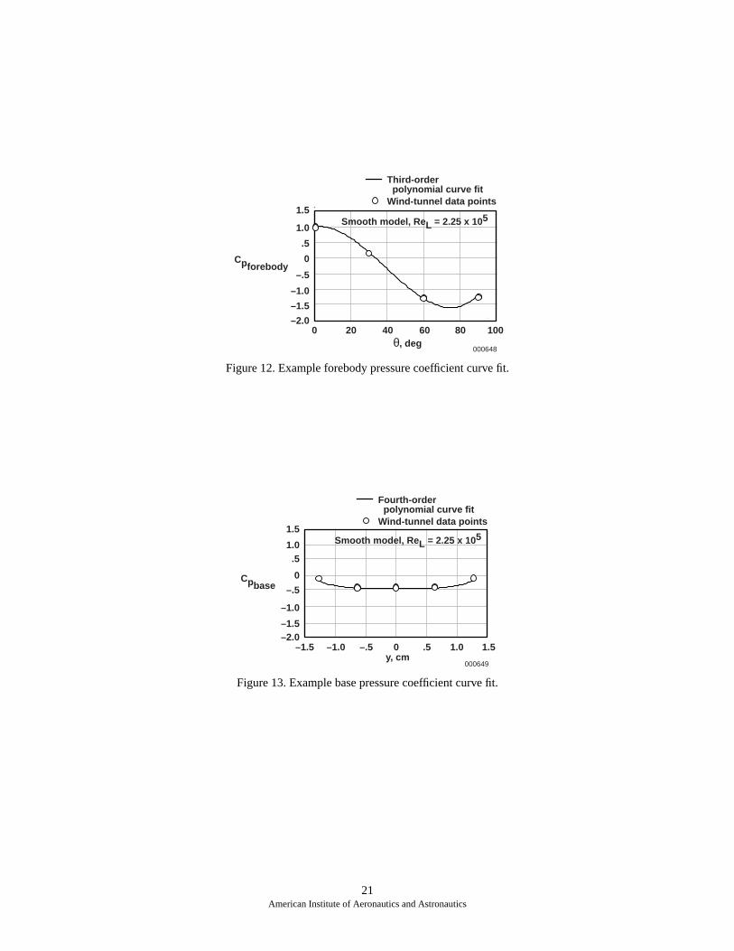
The forebody pressure coefficient was evaluated bycurve-fitting the pressure distributions as a function oflocal incidence angle, . For the forebody data, sevenforebody pressures—ports 1, 2, 3, 4, 14, 15, and 16(fig. 5)—are curve-fit with a third-order polynomial.The forebody pressure drag coefficient is analyticallygiven by the surface integral

(30)

Figure 12 shows a plot of a sample forebody curve fit.These smooth model data were measured with the windtunnel operating at . The forebodypressure coefficient data is plotted as a function of thelocal incidence angle. The upper and lower surfacepressure data lie nearly superimposed on each other, sonot surprisingly, the third-order curve-fit closelymatches the pressure coefficient data.

Base Pressure Analysis

The base pressure coefficient was evaluated bycurve-fitting the base pressure distributions as a functionof the lateral offset coordinate, . For the base pressuredata, five base area pressure ports—ports 7, 8, 9, 10, and11 (fig. 5)—were curve-fit with a fourth-orderpolynomial. The pressure ports on the sides of the model(ports 7 and 11) were included in the curve fit to account

for the taper of the base pressure near the outer edgethe model. In this curve-fitting scheme, ports 7 and were weighted one-half as much as the three base ports (ports 8, 9, and 10). This weighting scheme wselected to give a base drag taper correction factorapproximately 0.925. This correction factor is suggestby Saltzman, et al.5 for full-scale flight vehicles.

The base pressure drag coefficient is givanalytically by the evaluating the surface integral

(31)

Figure 13 shows a sample base pressure distribucurve fit. These data were measured on the smomodel with the wind tunnel operating at an approximaReynolds number of , based on model lengt

Results and Discussion

The wind-tunnel data clearly support the earlier CFpredictions that the smooth model will lie on thsuboptimal side of Hoerner’s curve. The suboptimhypothesis is most clearly demonstrated by examinthe base area pressure distributions. Figure 14 shthese results. The base pressure coefficients are plohere as a function of for various surface grid patterFigure 14(a) shows the pressure distributions f

and figure 14(b) shows the pressudistributions for . Interestingly, thesurface pattern with fine-mesh parallel slots and lancauses the base drag to dramatically rise (and hlower base pressure coefficients) when compared wthe smooth surface model. Conversely, the surfapattern with transverse slots and lands causes the bdrag to gradually lower (and have higher base presscoefficients) when compared to the smooth surfamodel.

A similar behavior was observed by Krishnan, et al.,14

when the authors added riblet15 structures to theforebody of an axisymmetric wind-tunnel model with blunt base. The authors’ intents were that the riblewould lower base drag; however, the results weopposite of expectations. When Krishnan’s results athe data presented in figure 14 are interpretconsidering Hoerner’s curve (fig. 3), the rising base dris completely reasonable. The grid pattern with paralslots and lands has the effect of acting like riblets on model forebody. The riblet structures have the effectlowering the forebody drag coefficient. Because t

HH 2 H+( )β+[ ]

--------------------------------------

L

CF1L--- 2

dθdx------ H

H 2 H+( )β+[ ]-------------------------------------- dx

0

L

∫=

2θL--- H

H 2 H+( )β+[ ]--------------------------------------≈

θ

CDforebodyCp θ[ ] cos θ[ ] θd

0

π 2⁄

∫=

aiθicos θ[ ]

i 0=

3

∑ θd0

π 2⁄

∫=

a0 0.5708 a1 0.4674a2 0.4510 a3++ +=

ReL 2.25 105×=

y

CDbaseCp y[ ] yd

0.5– ''

0.5''

∫ bi yi

0

4

∑ yd0.5– ''

0.5''

∫= =

b= 0 0.0833 b2 0.0125 b4+ +

2.25 105×

y

ReL 2.25 105× ,=ReL 1.25 10

5×=


ryhetoo,eagndge 2

nd-to-nalghlyurereacles

o-ach

actdyhese.eredhthe

ofseyry inte

onillg

othela

taing

enr

forebody skin drag coefficient is lowered, the base dragis expected to correspondingly increase. Clearly, ribletsshould not be used in conjunction with “suboptimal”configurations that have highly separated base regions;their effect will cause the base drag to rise.

Figure 15 shows results from the wind-tunnel teststhat further illustrate this concept. The measured basedrag coefficient is plotted with the viscous forebodydrag coefficient calculated from the boundary-layersurvey data. These data are compared to the curve fit ofHoerner’s two-dimensional data from figure 1. The opensymbols represent data for and theclosed symbols represent data for .The error bars show the expected “ ” standarddeviations based on the error analyses presented earlier.The agreement with the curve fit of Hoerner’s data isreasonably good.

Figure 16 shows the model total drag coefficient data(as calculated from the wake survey data) plotted withthe viscous forebody drag coefficient. The error barsshow the expected “ ” standard deviations based onthe error analyses presented earlier. Figure 16 alsoshows the predicted drag curve defined using Hoerner’stwo-dimensional curve from figure 1, the viscousforebody drag measurement, and the model forebodydrag coefficient predicted (–0.018) by the CFDsolutions. Note that, with the exception of the data forthe parallel grid (riblets) overlay, the agreement with thepredicted drag curve is very good.

The disagreement for the parallel grid test points is

caused by a sharp rise in the forebody pressure

coefficients. Figure 17 shows these data. The forebody

pressure distributions for all of the grids are plotted here

as a function of the local incidence angle. Figure 17(a)

shows the higher Reynolds number data

and figure 17(b) shows lower Reynolds number data

The transverse grid patterns do not

significantly alter the forebody pressure distribution;

however, the forebody pressure data are considerably

higher for the parallel grid pattern. The parallel grid data

are clearly an anomaly. The reasons for this pressure

anomaly are not clear at this point, but the parallel grid

possibly caused relaminarization of the flow and

induced a localized separation. This anomaly requires

further investigation.

Most importantly, the data shown in figure 16demonstrate the existence of a drag minimum withregard to the viscous forebody drag coefficient. The

elusive “drag bucket” is clearly defined and the primahypothesis of this paper is conclusively proven. Tdrag reduction from the smooth model configuration the optimum point is approximately 15 percent. Alscomparison of figure 15 with figure 16 shows that thbase drag coefficient corresponding to the total drcoefficient minimum lies somewhere between 0.225 a0.275. This value is a bit lower than the 0.25–0.30 ranpredicted by analysis of Hoerner’s original data (figs.and 3).

Summary and Concluding Remarks

Current designs of transatmospheric crew return areusable launch vehicles have extremely large basewetted area ratios when compared to conventiovehicle designs. These truncated base areas are hiseparated, resulting in large, negative, base presscoefficients. Because of the large base-to-wetted-aratio, base drag makes up the majority of overall vehidrag. Any reduction in base drag directly improvevehicle performance, resulting in an enhanced lift-tdrag ratio, extended range, and a less-severe approglide slope.

Early work performed on blunt-based bodies offerspotential solution. For blunt-based bodies, a direcorrelation exists between base and “viscous” forebodrag. As the forebody drag coefficient increases, tbase drag of the projectile generally tends to decreaThis base drag reduction results from boundary-layeffects at the vehicle base. Conceptually, if the addincrement in forebody skin drag is optimized witrespect to the base drag reduction, then reducing overall drag of the configuration may be possible.

In order to test the above concept, a series small-scale wind-tunnel tests was conducted. In thetests, a two-dimensional cylinder with a blunt afterbodwas tested. The series of tests had two primaobjectives: to test the forebody roughness hypothesisa systematic manner to conclusively demonstraexistence of a “drag bucket”; and to establish a criterifor when forebody drag is suboptimal (that is, when wincreasing forebody drag result in an overall drareduction).

This paper presents the wind-tunnel test results. Bprimary objectives were satisfied. These wind-tunnresults conclusively demonstrate existence of forebody drag optimum. Also, the wind-tunnel dademonstrate that the base drag coefficient correspondto the total drag minimum lies somewhere betwe0.225 and 0.275. This optimality point is slightly lowe

ReL 2.25 105×=

ReL 1.25 105×=

1-σ

1-σ

2.25 105×( ),

1.25 105×( ).


ehehe

isalnd

agedel

than the 0.25–0.30 range predicted by analysis ofHoerner’s original data. The use of parallel grid linesthat emulate the effects of riblet structures on bodieswith highly separated base regions will likely cause thetotal drag of the configuration to rise. Most importantly,the data show a peak drag reduction was approximately15 percent. When this 15-percent drag reduction isscaled to the size of the X-33 vehicle, the drag savingsapproaches approximately 45,000 N (10,000 lbf).

Clearly, this experiment should be repeated fordifferent ranges of Reynolds number and aspect ratios todetermine if the lower optimality point indicated by thedata is real. The methods should also be demonstrated asbeing effective in the presence of induced drag. Practical

implementation methods that allow for on-line adaptivmodification of the forebody drag coefficient to seek toptimal point should be explored and developed. Tlimits of practical applicability for this technology areunknown at this point. This drag reduction technologystill in its infancy; however, a wide spectra of potentiusers exist, including the aerospace, automotive, groutransport, and shipping industries. Use of this drreduction technique offers the potential for decreasoperating costs resulting from decreased overall fuconsumption.


Figure 1. The effect of the viscous forebody drag on the base drag of a blunt-based projectile.

CDbase

CF

.8

.7

.6

.5

.4

.3

.2

.1

Two-dimensional data (from Hoerner)Two-dimensional curve fitThree-dimensional data (from Hoerner)Three-dimensional curve fit

0 0.5 1.0 1.5 2.0

000636

CD base = 0.0974[CF]–0.4064

CD base = 0.029[CF]–0.5


Figure 2. Schematic depiction of the predicted “drag bucket.”

Figure 3. Comparison of flight data to two- and three-dimensional drag models.

CF

CF +

CDbase

0

.2

Drag bucket

.4

.6

.8

.2 .4 .6 .8 1.0

000637

Two-dimensional drag optimizationThree-dimensional drag optimization

X-15

M2-F3

X24-B

X24-B

Shuttle Enterprise

X-15X-33

X-33

CF

CD

0

.1

.2

.3

.4

.5

.6

.7

.8

.10.01 1.00

000638

HL-10

HL-10

M2-F1

M2-F1

X24-A

X24-A

M2-F3

Drag coefficientsBase (two-dimensional model)Total (two-dimensional model)Base (three-dimensional model)Total (three-dimensional model)Base (flight data)Total (flight data)

Shuttle Enterprise


Figure 4. Von Karman “vortex street” formation trailing the M2-F1 vehicle.


(a) Three-view drawing.

Figure 5. Schematic of wind-tunnel model.

Side view30°

60°

1.27 cm (0.5 in.) radius

2.54 cm(1.0 in.)

Bar gridroughness

overlay

yθ

Tunnel walls

Tunnel walls

Mount pin

x

0.635 cm

(0.25 in.)

Pivot pin

Top view

Front view10.033 cm(3.95 in.)

3.81 cm(1.50 in.)

7.62 cm(3.0 in.) 3.493 cm

(1.375 in.)1.905 cm(0.75 in.)

12.7 cm(5.0 in.)

000640

10.16 cm(4.0 in.)


(b) Pressure port numbering scheme.

Figure 5. Schematic of wind-tunnel model. Concluded.

Figure 6. Base drag model mounted in wind tunnel.

Model top view, looking down

1615 14 13 12 11

1098

765432

1

000641


Figure 7. Bar grid surface overlay screen pattern.

0.1 in.

0.75 in.

2.25 in.

4.0 in.

0.1 in.

4.5 in.

Centerline

1.375 in.

Etched surface

Inset of bar grid pattern

τ

Σλ

Direction of flow

0.25 in. diameter border around port

000643


Figure 8. Dynamic pressure calibration to account for tunnel blockage.

Figure 9. Two-dimensional, incompressible CFD solutions of wind-tunnel model flow field (smooth configuration).

Axial position in tunnel, cm

Boundary-layerprobe location

Wake probe location

1.0

1.1

1.2

1.3

12

43 5 6 78

910

111213141516 Model top view,

looking down

.9 .9988

.9990

.9992

.9994

.9996

.9998

1.0000

1.0002

0 10 20 30 40

000644

q/q∞ p/p∞Dynamic pressure ratioStatic pressure ratio ReL ~ 2.25 x 105

Static pressure ratio ReL ~ 1.25 x 105

000645

Cpforebody ~ –0.018, Cpbase

~ –0.350

Periodic vortex

Base separation

Forebody suction

36.732

–14.580


Figure 10. Example wind-tunnel wake data.

Figure 11. Example wind-tunnel boundary-layer curve fit.

y, cm

Smooth model, ReL = 2.25 x 1051.02

1.00

.98

.96

.94

.92

.90–5.0 –2.5 0 2.5 5.0 7.5–7.5

000646

u(y)

Ue

Cosine curve fitMeasured data

y/δ

1.1

1.0

.9

.8

.7

.6.001 .01 .10 1.00

000647

Smooth model, ReL = 2.25 x 105

u(y)

Ue

δ = 0.6401 cm

Curve fit, Π = 1.032Curve fit, Π = 0.4261/7th power law fitWind-tunnel test data


Figure 12. Example forebody pressure coefficient curve fit.

Figure 13. Example base pressure coefficient curve fit.

θ, deg

1.0

.5

0

–.5

–1.0

–1.5

–2.0

1.5

Third-order polynomial curve fitWind-tunnel data points

1000 20 40 60 80

000648

Cpforebody


y, cm

–2.0–1.5

–1.0

–.5

0

.51.0

1.5

Fourth-order polynomial curve fitWind-tunnel data points

–1.5 –1.0 –.5 0 .5 1.0 1.5

000649

Cpbase


(a)

(b)

Figure 14. Base pressure distributions for various grid patterns.

y, cm

–.55

–.50

–.45

–.40

–.35

–.30

–.25

–.20

–.15

–2.50 –1.25 0 1.25 2.50

Parallel grid

Increasing levels of roughness

000650

Cpbase

Smooth modelTransverse grid 2, κs ~ 0.1143 cmTransverse grid 4, κs ~ 0.4854 cmParallel grid 1, κs ~ 0.0163 cmTransverse grid 3, κs ~ 0.2896 cmTransverse grid 5, κs ~ 0.6911 cm

ReL 2.25 105.×=

y, cm

–.50

–.45

–.40

–.35

–.30

–.25

–.20

–.15

–2.50 –1.25 0 1.25 2.50

Parallel grid

Increasing levels of roughness

000651

Cpbase


ReL 1.25 105.×=


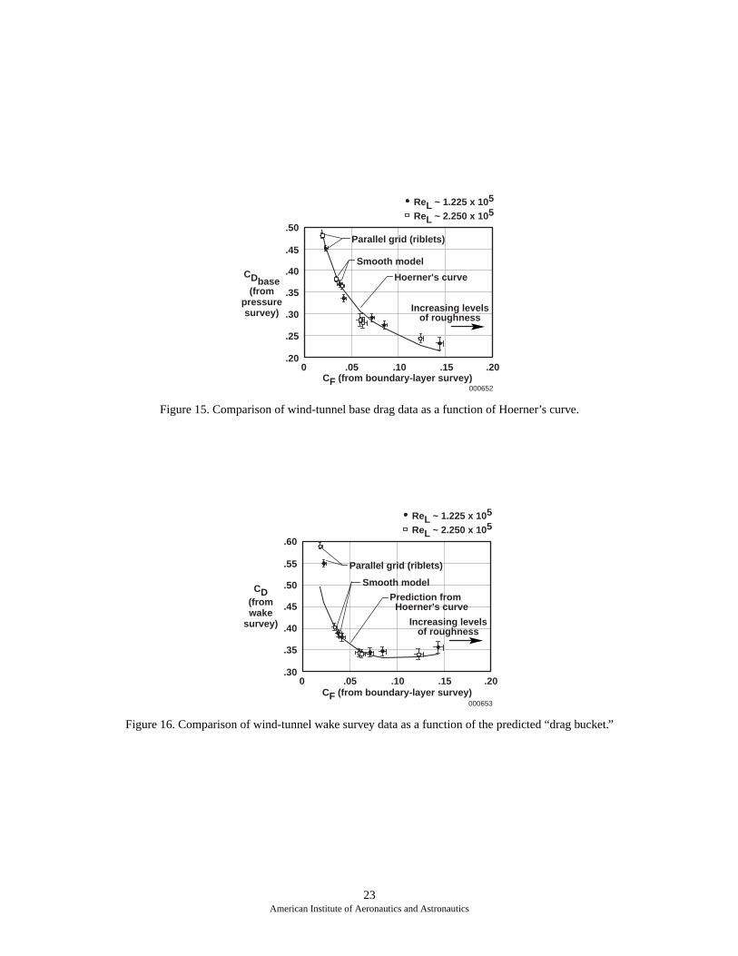
Figure 15. Comparison of wind-tunnel base drag data as a function of Hoerner’s curve.

Figure 16. Comparison of wind-tunnel wake survey data as a function of the predicted “drag bucket.”

Smooth model

Parallel grid (riblets)

Increasing levelsof roughness

Hoerner's curve

CF (from boundary-layer survey)

.50

.45

.40

.35

.30

.25

.20.20.15.10.050

000652

CDbase(from

pressuresurvey)

ReL ~ 1.225 x 105

ReL ~ 2.250 x 105

Smooth model

Parallel grid (riblets)

Increasing levelsof roughness

Prediction from Hoerner's curve

.60

.55

.50

.45

.40

.35

.30.20.15.10.050

000653

ReL ~ 1.225 x 105

ReL ~ 2.250 x 105

CF (from boundary-layer survey)

CD(fromwake

survey)



(a)

(b)

Figure 17. Forebody pressure distributions for various grid patterns.

θ, deg

–2

–1

0

1

2

0 20 40 60 80 100

Parallel grid

Smooth model and transverse grids

000654

Cpforebody


ReL 2.25 105.×=

θ, deg

–2

–1

0

1

2

0 20 40 60 80 100

Parallel grid

Smooth model and transverse grids

000655

Cpforebody


ReL 1.25 105× .=

tyn

ity

e

dter

APPENDIXERROR ANALYSIS METHODS

Introduction

An approximate accounting of overall error in thewind tunnel–derived drag coefficient estimates isderived herein. The wake error analysis is presentedfirst; the boundary-layer skin-friction error analysis ispresented next. The estimated errors in the forebody andbase pressure drag coefficients are presented last. Theerror equations derived in this appendix were used tocalculate the data point error bounds plotted in figures15 and 16.

Estimating the Wake Drag Coefficient Errors

An approximate accounting of overall error in thewake drag coefficient can be performed using a linearperturbation analysis. Using the fundamental definitionfor momentum thickness, linear perturbations can beexpressed in terms of the velocity profile curve-fit error

by taking the first variation of the forebody

surface incidence angle, , with respect to :

(A-1)

The mean-square error in momentum thickness isevaluated by taking the expectation of the square ofequation (A-1).

(A-2)

Assuming that random local errors in the velociprofile curve fit are uncorrelated, the expectatiooperation in equation (A-2) becomes

(A-3)

In equation (A-3), is the Dirac delta function16

and is the mean-square error in the veloc

distribution curve fit. Substituting equation (A-3) intoequation (A-2), the interior integral reduces to thfollowing:

(A-4)

Substituting equation (A-4) into equation (A-2), anusing the wake cosine law (eq. (2)) to evaluate the ou

u y( )Ue

-----------∆

θ u y( ) Ue⁄

∆θ ∆u y( ) Ue⁄u y( )Ue

----------- 1 u y( )Ue

-----------– ydδ–

δ

∫≈

δ ∆u ξ( )Ue

-----------1 2

u ξ( )Ue

-----------– ξd1–

1

∫=

Ψ2∆θw

E ∆θ2[ ]=

δ2E ∆ uξ

Ue------ 1 2

u ζ( )Ue

-----------–

1–1∫ dξ=

∆u ζ( )Ue

----------- 1 2u ζ( )Ue

-----------–

ζd1–

1

∫×

δ2E ∆u ξ( )

Ue-----------∆u ζ( )

Ue----------- 1 2

u ξ( )Ue

-----------–

1–

1

∫1–

1

∫×

1 2u ζ( )Ue

-----------–

ζd ξd×

E ∆u ξ( )Ue

-----------∆u ζ( )Ue

-----------

0 when ξ ζ≠

Ψ2∆u Ue⁄ when ξ ζ=

=

Ψ2∆u Ue⁄ Λξ ζ,=

Λξ ζ,

Ψ2∆u Ue⁄

E ∆u ξ( )Ue

-----------∆u ζ( )Ue

----------- 1 2u ξ( )Ue

-----------–

1–

1

∫

1 2u ζ( )Ue

-----------–

ζd

Ψ2∆u Ue⁄ 1 2

u ζ( )Ue

-----------–2

=


ror

ne

us

agurealnd

integral, the approximate mean-square error in themomentum thickness reduces to the following:

(A-5)

A first-order perturbation of equation (A-5) gives theerror equation for the free-stream momentum thicknessestimate (assuming that errors in the velocity ratio andshape parameter are negligible when compared to themomentum thickness errors):

(A-6)

Finally, the approximate mean square error in totaldrag coefficient is

(A-7)

In equation (20), is the shape parameter defined by

equation (10), is the boundary-layer thickness, and

is the mean-square error in the velocity

profile curve fit.

Estimating the Forebody Viscous Drag Coefficient Errors

The boundary-layer error analysis follows a nearlyidentical process when compared to the wake erroranalysis. The main exceptions are that the integrals areperformed from instead of , and thevelocity distribution is given by the law of the wakeinstead of the cosine law velocity distribution. Keeping

these differences in mind, the mean-squared erformula for the momentum thickness becomes

(A-8)

Substituting the law-of-the-wake velocity distributio(eq. (16)) into equation (A-8) and integrating gives thmean-square error in momentum thickness:

(A-9)

The corresponding mean-square error in the viscoforebody drag coefficient estimate is

(A-10)

Estimating the Forebody Drag Coefficient Errors

For each configuration, the forebody pressure drcoefficient errors are approximated using the presscoefficient standard deviations from the ten individutrials. For each pressure port location, , the mean avariance in pressure coefficients are computed as

Ψ2∆θw

δ2 Ψ2

∆u Ue⁄ 3umin

Ue----------

22

umin

Ue----------– 1+=

Ψ2∆θ∞

Ψ2∆θw

Ue

U∞--------

H 5+[ ]=

δ2 Ψ2

∆u Ue⁄Ue

U∞--------

H 5+[ ]=

3umin

Ue----------

22

umin

Ue----------– 1+×

Ψ2CD0

4Ψ2

∆θ∞

hbase2

----------------=

4δ2

Ψ2∆u Ue⁄

hbase2

-------------------------------Ue

U∞--------

H 5+[ ]=

3umin

Ue----------

22

umin

Ue----------– 1+×

H

δ

Ψ2∆u Ue⁄

0 δ,{ } δ δ,–{ }

Ψ2∆θw

E ∆θ2[ ]=

δ2=

E ∆ u ξ( )Ue

----------- 1 2u ξ( )Ue

-----------–

ξ ∆ u ζ( )Ue

----------- 1 2u ζ( )Ue

-----------–

ζd0

1

∫d0

1

∫δ2

Ψ2∆u Ue⁄ 1 2

u ξ( )Ue

-----------–2

ξd0

1

∫×

Ψ2∆θ

δ2Ψ2∆u Ue⁄

πκ2----------------------------------=

πκ22 2c f x

π 4Π+[ ]κ– 4c f x+ π 5.48304 Π πΠ2

+ +[ ]×

Ψ2CF

2L--- H

H 2 H+( )β+[ ]--------------------------------------

2=

δ2Ψ2∆u Ue⁄

πκ2----------------------------------×

πκ22 2c f x

π 4Π+[ ]κ– 4c f x+ π 5.48304 Π πΠ2

+ +×

θ j


ars.dereats asrts):

(A-11)

and

(A-12)

Based on equation (30), which is a pressure integralweighted by the cosine of the local incidence angle,mean-square error in forebody drag coefficient iscomputed as the sum-square of individual forebodypressure coefficient errors, weighted by the cosine of thelocal incidence angle.

(A-13)

Estimating the Base Drag Coefficient Errors

The base drag coefficient errors are computed insimilar manner as the forebody drag coefficient erroHowever, instead of weighting the standardeviations using , the weighting procedurfollows the scheme used to establish the base acurve fits (that is, the variances in the two poralong the sides of the model are weighted one-halfmuch as the variances in the three base-area po

(A-14)

µθ

Cpiθ( )

i 1=

Ntrials

∑Ntrials

----------------------------=

σθ2

Cpiθ( ) µθ–[ ] 2

i 1=

Ntrials

∑Ntrials 1–

------------------------------------------------=

Ψ2CD forebody

σθcosθ2[ ]i 1=

7

∑=

Cpcos θ[ ]

Cp

Cp

Ψ2CDbase

12---σ

sidei

2σbasei

2

i 1=

3

∑+i 1=

2

∑4

---------------------------------------------------------------------------=


ds,

e

ee

g

in

r,,”

g

References

1Wong, Thomas J., Charles A. Hermach, John O.Reller, Jr., and Bruce E. Tinling, “Preliminary Studies ofManned Satellites—Wingless Configurations: LiftingBody,” NACA Conference on High-SpeedAerodynamics: A Compilation of the Papers Presented,NASA TM-X-67369, 1958, pp. 35–44.

2Hoerner, Sighard F., Fluid-Dynamic Drag: PracticalInformation on Aerodynamic Drag and HydrodynamicResistance, Self-published work, Library of CongressCard Number 64-19666, Washington, D.C., 1965.

3Tanner, M., “Theories for Base Pressure inIncompressible Steady Base Flow,” Progress inAerospace Sciences, vol. 34, 1998, pp. 423–480.

4Rathakrishnan, E., “Effect of Splitter Plate on BluffBody Drag,” AIAA Journal, vol. 37, no. 9, Sept. 1999,pp. 1125–1126.

5Saltzman, Edwin J., K. Charles Wang, and KennethW. Iliff, “Flight-Determined Subsonic Lift and DragCharacteristics of Seven Lifting-Body and Wing-BodyReentry Vehicle Configurations With Truncated Bases,”AIAA-99-0383, Jan. 1999.

6Whitmore, Stephen A. and Timothy R. Moes, “ABase Drag Reduction Experiment on the X-33 LinearAerospike SR-71 Experiment (LASRE) FlightProgram,” AIAA-99-0277, Jan. 1999.

7Mills, Anthony F., Heat and Mass Transfer, IrwinPublishing Co., Burr Ridge, IL, 1995.

8Adaptive Research, CFD 2000: ComputationalFluid Dynamics System Version 2.2 User’s Manual,Pacific-Sierra Research Corporation, 1995.

9Rade, Lennart and Bertil Westergren, Beta

Mathematics Handbook: Concepts, Theorems, Metho

Algorithms, Formulas, Graphs, Tables, 2nd ed., CRCPress, Boca Raton, FL, 1990.

10White, Frank M, Viscous Fluid Flow, 2nd ed.,McGraw-Hill, New York, 1991.

11Coles, Donald, “The Law of the Wake in thTurbulent Boundary Layer,” Journal of Fluid

Mechanics, vol. 1, 1955, pp. 191–226.

12Whitmore, Stephen A., Marco Hurtado, JosRivera, and Jonathan W. Naughton, “A Real-TimMethod for Estimating Viscous Forebody DraCoefficients,” AIAA-2000-0781, Jan. 2000 (alsoavailable as NASA TM-2000-209015).

13Clauser, Francis H., “Turbulent Boundary Layers Adverse Pressure Gradients,” Journal of Aeronautical

Sciences, vol. 21, no. 2, Jan. 1954, pp. 91–108.

14Krishnan, V., P. R. Viswanath, and S. Rudrakuma“Effects of Riblets on Axisymmetric Base PressureJournal of Spacecraft and Rockets, vol. 34, no. 2,March–April 1997, pp. 256–258.

15Walsh, Michael J., “Riblets as a Viscous DraReduction Technique,” AIAA Journal, vol. 21, no. 4,Apr. 1983, pp. 485–486.

16Freiberger, W. F., ed., The International Dictionary

of Applied Mathematics, Van Nostrand Company, Inc.,Princeton, NJ, 1960.


REPORT DOCUMENTATION PAGE Form ApprovedOMB No. 0704-0188

Public reporting burden for this collection of information is estimated to average 1 hour per response, including the time for reviewing instructions, searching existing data sources, gathering andmaintaining the data needed, and completing and reviewing the collection of information. Send comments regarding this burden estimate or any other aspect of this collection of information,including suggestions for reducing this burden, to Washington Headquarters Services, Directorate for Information Operations and Reports, 1215 Jefferson Davis Highway, Suite 1204, Arlington,VA 22202-4302, and to the Office of Management and Budget, Paperwork Reduction Project (0704-0188), Washington, DC 20503.

1. AGENCY USE ONLY (Leave blank) 2. REPORT DATE 3. REPORT TYPE AND DATES COVERED

4. TITLE AND SUBTITLE 5. FUNDING NUMBERS

6. AUTHOR(S)

8. PERFORMING ORGANIZATION REPORT NUMBER

7. PERFORMING ORGANIZATION NAME(S) AND ADDRESS(ES)

9. SPONSORING/MONITORING AGENCY NAME(S) AND ADDRESS(ES) 10. SPONSORING/MONITORING AGENCY REPORT NUMBER

11. SUPPLEMENTARY NOTES

12a. DISTRIBUTION/AVAILABILITY STATEMENT 12b. DISTRIBUTION CODE

13. ABSTRACT (Maximum 200 words)

14. SUBJECT TERMS 15. NUMBER OF PAGES

16. PRICE CODE

17. SECURITY CLASSIFICATION OF REPORT

18. SECURITY CLASSIFICATION OF THIS PAGE

19. SECURITY CLASSIFICATION OF ABSTRACT

20. LIMITATION OF ABSTRACT

NSN 7540-01-280-5500 Standard Form 298 (Rev. 2-89)Prescribed by ANSI Std. Z39-18298-102

Wind-Tunnel Investigations of Blunt-Body Drag Reduction UsingForebody Surface Roughness

718-20-00-E8-53-00-b52

Stephen A. Whitmore, Stephanie Sprague, and Jonathan W. Naughton

NASA Dryden Flight Research CenterP.O. Box 273Edwards, California 93523-0273

H-2439

National Aeronautics and Space AdministrationWashington, DC 20546-0001 NASA/TM-2001-210390

This paper presents results of wind-tunnel tests that demonstrate a novel drag reduction technique for blunt-basedvehicles. For these tests, the forebody roughness of a blunt-based model was modified using micomachined surfaceoverlays. As forebody roughness increases, boundary layer at the model aft thickens and reduces the shearing effect ofexternal flow on the separated flow behind the base region, resulting in reduced base drag. For vehicle configurations withlarge base drag, existing data predict that a small increment in forebody friction drag will result in a relatively large decreasein base drag. If the added increment in forebody skin drag is optimized with respect to base drag, reducing the total dragof the configuration is possible. The wind-tunnel tests results conclusively demonstrate the existence of a forebody drag–base drag optimal point. The data demonstrate that the base drag coefficient corresponding to the drag minimum liesbetween 0.225 and 0.275, referenced to the base area. Most importantly, the data show a drag reduction of approximately15 percent when the drag optimum is reached. When this drag reduction is scaled to the X-33 base area, drag savingsapproaching 45,000 N (10,000 lbf) can be realized.

Base drag, Drag reduction, Reusable launch vehicle, Skin friction, Wind tunnel

A03

34

Unclassified Unclassified Unclassified Unlimited

January 2001 Technical Memorandum

Presented at 39th AIAA Aerospace Sciences Meeting and Exhibit, Reno, Nevada, January 8–11, 2001,AIAA-2001-0252. Stephanie Sprague, University of Kansas. Jonathan W. Naughton, University of Wyoming.

Unclassified—UnlimitedSubject Category 05

This report is available at http://www.dfrc.nasa.gov/DTRS/

Documents

Wind-Tunnel Investigations of Blunt-Body Drag Reduction ... · the base area. Most importantly, the data show a drag reduction of approximately 15 percent when the drag optimum is