Embed Size (px)
Citation preview
Loughborough UniversityInstitutional Repository
Novel methods of dragreduction for squareback
road vehicles
This item was submitted to Loughborough University's Institutional Repositoryby the/an author.
Additional Information:
• A Doctoral Thesis. Submitted in partial fulfilment of the requirementsfor the award of Doctor of Philosophy of Loughborough University.
Metadata Record: https://dspace.lboro.ac.uk/2134/12534
Publisher: c© Rob Littlewood
Please cite the published version.

This item was submitted to Loughborough University as a PhD thesis by the author and is made available in the Institutional Repository
(https://dspace.lboro.ac.uk/) under the following Creative Commons Licence conditions.
For the full text of this licence, please go to: http://creativecommons.org/licenses/by-nc-nd/2.5/
Novel Methods of Drag Reduction for Squareback Road Vehicles
Rob Littlewood Page i
NOVEL METHODS OF DRAG REDUCTION FOR
SQUAREBACK ROAD VEHICLES
BY ROB LITTLEWOOD
DOCTORAL THESIS
SUBMITTED IN PARTIAL FULFILLMENT OF THE REQUIREMENTS
FOR THE AWARD OF DOCTOR OF PHILOSOPHY OF
LOUGHBOROUGH UNIVERSITY
APRIL 2013
© R.P.LITTLEWOOD 2013
Novel Methods of Drag Reduction for Squareback Road Vehicles
Rob Littlewood Page ii
ABSTRACT
Road vehicles are still largely a ‘consumer product’ and as such the styling of a vehicle becomes a
significant factor in how commercially successful a vehicle will become. The influence of styling
combined with the numerous other factors to consider in a vehicle development programme means
that the optimum aerodynamic package is not possible in real world applications.
Aerodynamicists are continually looking for more discrete and innovative ways to reduce the drag of
a vehicle. The current thesis adds to this work by investigating the influence of active flow control
devices on the aerodynamic drag of square back style road vehicles. A number of different types of
flow control are reviewed and the performance of synthetic jets and pulsed jets are investigated on a
simple 2D cylinder flow case experimentally.
A simplified ¼ scale vehicle model is equipped with active flow control actuators and their effects on
the body drag investigated. The influence of the global wake size and the smaller scale in-wake
structures on vehicle drag is investigated and discussed. Modification of a large vortex structure in
the lower half of the wake is found to be a dominant mechanism by which model base pressure can be
influenced. The total gains in power available are calculated and the potential for incorporating active
flow control devices in current road vehicles is reviewed. Due to practicality limitations the active
flow control devices are currently ruled out for implementation on a road vehicle.
The knowledge gained about the vehicle model wake flow topology is later used to create drag
reductions using a simple and discrete passive device. The passive modifications act to support
claims made about the influence of in wake structures on the global base pressures and vehicle drag.
The devices are also tested at full scale where modifications to the vehicle body forces were also
observed.

Novel Methods of Drag Reduction for Squareback Road Vehicles
Rob Littlewood Page iii
ACKNOWLEDGEMENTS
I would like to thank my supervisor Martin Passmore for his continued support from when I was an
undergraduate student and throughout my postgraduate studies. I would also like to thank Rob Hunter
and Stacey Prentice for their work to keep the wind tunnel running and supply me with various
incarnations of wind tunnel models and components. Thanks also go to all my fellow PhD students,
undergraduate students and staff within the Aeronautical and Automotive Engineering Department at
Loughborough University who helped along the way.
I would also like to thank Jeff Howell for the wealth of advice he provided on automotive bluff body
testing, and Adrian Gaylard at Jaguar Land Rover for his continued interest and support of the work.
Finally thanks go to my fiancé, parents and whole family for their continued support and patience.

Novel Methods of Drag Reduction for Squareback Road Vehicles
Rob Littlewood Page iv
Nomenclature
A Frontal area (m2)
a Sensor temperature coefficient
a0 Overheat ratio
Ad Coefficient of tyre resistance (static)
APNET Net change in aerodynamic power (W)
ASC Acoustic streaming criterion
At Coefficient of transmission resistance (static)
Au Coefficient of undriven wheel resistance (static)
b Jet characteristic length (Hole: diameter, Slot: width) (m)
Bd Coefficient of tyre resistance (dynamic)
Bt, Ct Coefficients of transmission resistances (dynamic)
Bu Coefficient of undriven wheel resistance (dynamic)
Cµ Jet momentum coefficient
Cb Pressure contributions from base
Cd Coefficient of drag
CF Coefficient of force
Cf Pressure contributions from skin friction
CFD Computational fluid dynamics
Ck Pressure contributions from front of model
Cl Coefficient of lift
Clr Coefficient of rear lift
Cp Coefficient of pressure
Area weighted pressure coefficient
Cs Pressure contributions from slant
D Model characteristic length scale (m)
d Displacement (m)
E Blockage ratio
eµ Statistical accuracy
Ea Applied voltage
Ecorr Corrected applied voltage
f Frequency (Hz)
F+ Reduced actuation frequency, (usually a multiple of a characteristic
shedding frequency)

Novel Methods of Drag Reduction for Squareback Road Vehicles
Rob Littlewood Page v
FDRAG Drag force (N)
FoV Field of view
FTR Tractive resistance
g Gravity (9.81)
H Characteristic length/ height (m)
IO Jet momentum
L Characteristic length (m)
Ladvec Advection length (m)
LDA Laser doppler annemometry
Mass flow rate (kg/s)
M Vehicle mass (Kg)
MSBC Moving surface boundary layer control
N Number of samples
P Pressure (Pa)
p Pressure local to tapping measurement (Pa)
p∞ Reference pressure in freestream (Pa)
PAERO Aerodynamic power (W)
PIV Particle image velocimetry
q Freestream dynamic pressure (Pa)
R Specific gas constant for air (287)
Re Reynold's number
ReI0 Jet Reynold's number
RMS Root mean squared
sd Standard deviation of displacement (m)
SJ Synthetic jet
st Standard deviation of time (s)
St Strouhal number
Stact Actuation Strouhal number
STOL Short take off and landing
sv Standard deviation of velecity (m/s)
T Temperature (K)
t Time (s)
t* distribution factor for a given confidence level
T0 Ambient temperature at the time of setting the overheat

Novel Methods of Drag Reduction for Squareback Road Vehicles
Rob Littlewood Page vi
Ta Ambient temperature at the time of sampling
Tw Hot wire sensor operating voltage
U∞ Freestream velocity (m/s)
Uc Advection speed (m/s)
Uj Jet exit velocity (m/s)
V Velocity (m/s)
η Jet efficiency
μ Kinematic viscocity
Density (Kg/m3) (Air = 1.225)
j Jet fluid density (Kg/m3)
0 Freestream density (kg/m3)
Angle (degrees)
Novel Methods of Drag Reduction for Squareback Road Vehicles
Rob Littlewood Page vii
TABLE OF CONTENTS
Nomenclature ............................................................................................................... iv
1.0 Introduction ....................................................................................................... 2
1.1 Tractive Resistance ................................................................................................................ 3
1.2 Sources of Drag ..................................................................................................................... 4
1.2.1 Base Pressure and Vortex Drag ......................................................................................... 5
1.2.2 Rear edge conditioning...................................................................................................... 8
1.2.3 Drag Reduction Techniques .............................................................................................. 9
1.3 Drag Reduction Techniques; Passive .................................................................................... 9
1.3.1 Diffusers ............................................................................................................................ 9
1.3.2 Boat Tailing ..................................................................................................................... 10
1.3.3 Flaps and Plates ............................................................................................................... 12
1.4 Drag Reduction Techniques; Active .................................................................................... 14
1.4.1 Moving Surface Boundary Layer Control (MSBC) ........................................................ 14
1.4.2 Continuous Suction ......................................................................................................... 15
1.4.3 Continuous Blowing ........................................................................................................ 15
1.4.4 Synthetic Jet Actuators .................................................................................................... 18
1.5 Drag Reduction Techniques; Further Investigation ............................................................. 27
2.0 Experimental Method ..................................................................................... 30
2.1 Experimental Uncertainty .................................................................................................... 30
2.2 Wind Tunnel and Force Balance ......................................................................................... 31
2.3 Surface Pressure Measurement ............................................................................................ 33
Novel Methods of Drag Reduction for Squareback Road Vehicles
Rob Littlewood Page viii
2.4 Hot Wire Anemometry ........................................................................................................ 34
2.5 Particle Image Velocimetry ................................................................................................. 35
2.5.1 Seeding and Camera Field of View ................................................................................. 36
2.5.2 Image Acquisition ........................................................................................................... 37
2.5.3 Data Processing ............................................................................................................... 38
2.5.4 Post Processing ................................................................................................................ 39
2.5.5 PIV Resolution, Accuracy and Precision ........................................................................ 40
2.5.6 PIV Summary .................................................................................................................. 47
3.0 Baseline Vehicle Configuration and Passive Optimisation ......................... 49
3.1 Introduction ......................................................................................................................... 49
3.2 Force and Pressure Measurement Results ........................................................................... 52
3.3 PIV Results .......................................................................................................................... 58
3.4 Discussion and Implications for Further Work ................................................................... 65
4.0 Active Control Actuator Design and Testing ................................................ 68
4.1 Introduction ......................................................................................................................... 68
4.2 Initial Testing ....................................................................................................................... 70
4.2.1 Low Frequency Jet .......................................................................................................... 70
4.2.2 High Frequency Jet ......................................................................................................... 73
4.2.3 PIV and LDA Analysis of ‘Speaker Driven’ Synthetic Jet and Pneumatic Pulsed Jet ... 74
4.3 2D Cylinder Testing ............................................................................................................ 79
4.3.1 Experimental Setup ......................................................................................................... 79
4.3.2 Results; Pressure Measurements ..................................................................................... 81
Novel Methods of Drag Reduction for Squareback Road Vehicles
Rob Littlewood Page ix
4.4 Results; Balance Measurements .......................................................................................... 86
4.5 Discussion ............................................................................................................................ 88
5.0 Active Control Constant Blowing – Experiments, Results and Discussion 91
5.1 Model ................................................................................................................................... 91
5.2 Slot Exit Velocity Measurements ........................................................................................ 93
5.2.1 Jet Characterisation ......................................................................................................... 94
5.3 Force Measurements ............................................................................................................ 96
5.4 Pressure Measurements ....................................................................................................... 97
5.5 PIV ....................................................................................................................................... 97
5.6 Results – Balance Measurements ........................................................................................ 98
5.7 Results - Pressure Measurements ...................................................................................... 101
5.8 Results - PIV ...................................................................................................................... 103
5.9 Net Drag Changes .............................................................................................................. 109
5.10 Discussion .......................................................................................................................... 111
6.0 Active Control Pulsed Blowing – Experiments, Results and Discussion .. 114
6.1 Introduction ....................................................................................................................... 114
6.2 Model ................................................................................................................................. 114
6.3 Jet Characterisation............................................................................................................ 117
6.4 Balance Results ................................................................................................................. 120
6.5 PIV ..................................................................................................................................... 123
6.5.1 Configuration B ............................................................................................................. 124
6.5.2 Configuration C ............................................................................................................. 127
Novel Methods of Drag Reduction for Squareback Road Vehicles
Rob Littlewood Page x
6.5.3 Configuration D ............................................................................................................ 130
6.6 Discussion .......................................................................................................................... 132
7.0 Passive Control of In Wake Structures – Experiments, Results and
Discussion .................................................................................................................. 135
7.1 Introduction ....................................................................................................................... 135
7.2 Experimental Configurations ............................................................................................. 135
7.2.1 Model Scale ................................................................................................................... 135
7.2.2 Full Scale Vehicle Testing ............................................................................................ 136
7.3 Experimental Results ......................................................................................................... 139
7.3.1 Model Scale ................................................................................................................... 139
7.3.2 Full Scale ....................................................................................................................... 143
7.4 Discussion .......................................................................................................................... 145
8.0 Conclusions and Further Work ................................................................... 148
9.0 References ...................................................................................................... 151
Novel Methods of Drag Reduction for Squareback Road Vehicles
Rob Littlewood Page xi
Table of Figures
Figure 1.1 - Forces opposing the motion of a typical road vehicle (Ford Escort) ........................................... 2
Figure 1.2 - Percentage contributions of resistive forces contributing to Equation 1 (Ford Escort) ............. 3
Figure 1.3 Wake sizes of different vehicle shapes (Heisler, 2002)..................................................................... 5
Figure 1.4 - Effect of backlight angle on Cd (Barnard, 1996)............................................................................ 6
Figure 1.5 - Isosurfaces of zero total pressure on Ahmed car model for increasing back angle (Keating,
Shock and Chen, 2008) ............................................................................................................................... 7
Figure 1.6 - Variation of drag with base slant angle (Ahmed, Ramm and Faltin, 1984) ................................ 7
Figure 1.7 - Drag due to large trailing radii (Kee, Kim and Lee, 2001) ........................................................... 8
Figure 1.8 - Audi A2 rear spoiler configuration ................................................................................................. 9
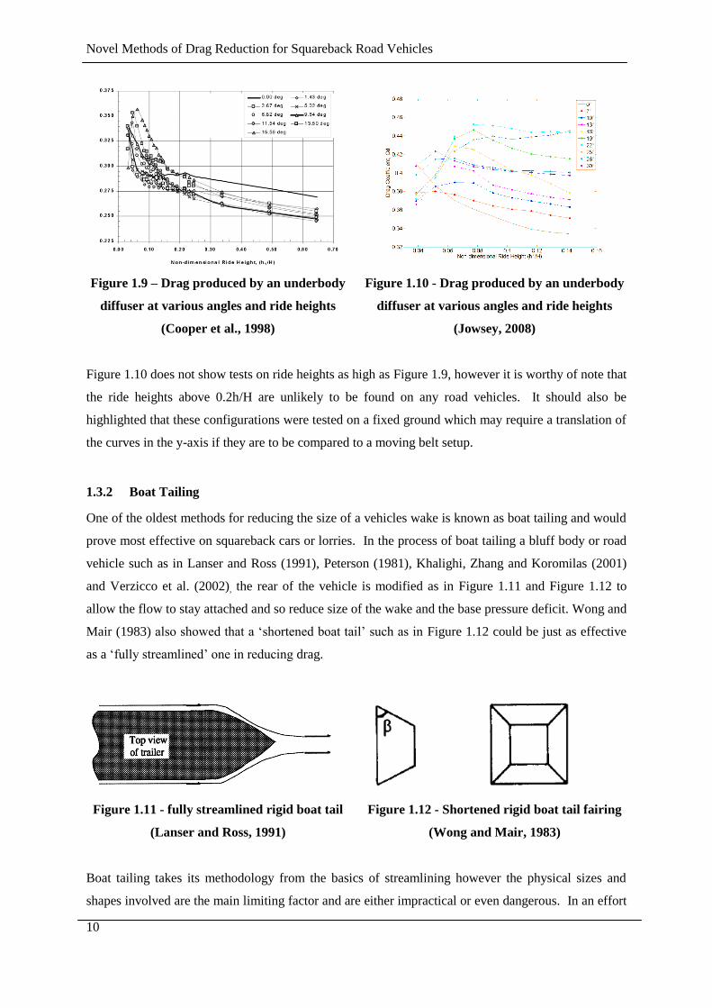
Figure 1.9 – Drag produced by an underbody diffuser at various angles and ride heights (Cooper et al.,
1998) ........................................................................................................................................................... 10
Figure 1.10 - Drag produced by an underbody diffuser at various angles and ride heights (Jowsey, 2008)
.................................................................................................................................................................... 10
Figure 1.11 - fully streamlined rigid boat tail (Lanser and Ross, 1991) ......................................................... 10
Figure 1.12 - Shortened rigid boat tail fairing (Wong and Mair, 1983) ......................................................... 10
Figure 1.13 - Boat tailing using extension plates (Khalighi, Zhang and Koromilas, 2001) .......................... 11
Figure 1.14 - Pressure coefficient at rear of bluff body left: standard setup right: with extension plates
(Khalighi, Zhang and Koromilas, 2001) .................................................................................................. 11
Figure 1.15 - 2D bluff body incorporating splitter plates of various lengths (Bearman, 1965).................... 12
Figure 1.16 - Spanwise base pressure distribution. x = without splitter plate and end plates, o = without
splitter plates but with end plates, □ = with splitter plate but without end plates (Bearman, 1965) . 12
Figure 1.17 - Rear Flap configuration for drag reduction (Kowata et al., 2008) .......................................... 13
Figure 1.18 - Flaps model (Beaudoin and Aider, 2008) ................................................................................... 13
Figure 1.19 - PIV vortex reduction (Beaudoin and Aider, 2008) .................................................................... 14
Figure 1.20 – Moving surface boundary layer control on a bluff body (Roumeas, 2006) ............................ 15
Figure 1.21 - Effect of continuous suction on Ahmed car (Roumeas, 2006) .................................................. 15
Figure 1.22 - Blowing technique on a wing (Englar, 2003).............................................................................. 16
Figure 1.23 – Continuous blowing at various angles into the wake of a bluff body (Rouméas, Gilliéron and
Kourta, 2006) ............................................................................................................................................. 17
Figure 1.24 - Synhetic Jet Illustration (Glezer and Amitay, 2002) ................................................................. 18
Novel Methods of Drag Reduction for Squareback Road Vehicles
Rob Littlewood Page xii
Figure 1.25 - Variation of the pressure coefficient around a tube with increasing dimensionless actuation
frequency SrD act = •;0.24, Δ;0.50, *; 0.83 and -; base line flow (Glezer, Amitay and Honahan, 2005)
.................................................................................................................................................................... 19
Figure 1.26 - Pressure distribution around 2D cylinder: unactuated with laminar BL, ○ unactuated
with tripped turbulent BL, ● actuated with tripped turbulent BL (Glezer, Amitay and Honahan,
2005) ........................................................................................................................................................... 20
Figure 1.27 - Pressure distribution around 2D cylinder: ● unactuated, tripped tur4bulent BL, (thin)
low level actuation, tripped turbulent BL, (thick) high level actuation, tripped turbulent BL (Béra
et al., 2000) ................................................................................................................................................. 20
Figure 1.28 – Velocity vectors and rotational intensity (Béra et al., 2000) .................................................... 21
Figure 1.29 - 2D diffuser (Brunn and Nitsche, 2006) ....................................................................................... 22
Figure 1.30 - Model configuration (Leclerc and Levallois, 2006) ................................................................... 22
Figure 1.31 - Cd vs reduced actuator frequency F+ (Leclerc and Levallois, 2006)....................................... 22
Figure 1.32 - D-Shaped body used in vortex suppression experiments (Pastoor et al., 2008) ...................... 23
Figure 1.33 – Instantaneous pressure distribution and wake flow distribution behind a D shaped bluff
body, without control (Pastoor et al., 2008) ............................................................................................ 24
Figure 1.34 - Instantaneous pressure distribution and wake flow distribution behind a D shaped bluff
body, controlled by SJ actuators (Pastoor et al., 2008) .......................................................................... 24
Figure 1.35 – Velocity vector plots at different actuator frequency F+ (Amitay and Glezer, 2002) ........... 25
Figure 1.36 - Recirculation bubble and shape .................................................................................................. 26
Figure 1.37 - Jet vectoring (Smith and Glezer, 2002) ...................................................................................... 26
Figure 2.1 - Loughborough University Wind Tunnel ...................................................................................... 31
Figure 2.2 - Example of drag coefficient measurement for a road car bluff ................................................. 33
Figure 2.3 - Pressure scanner and CanDaq ..................................................................................................... 33
Figure 2.4 - Jet velocity measurement using hot wire ..................................................................................... 34
Figure 2.5 – Typical PIV configuration (Raffel et al., 2007) ........................................................................... 35
Figure 2.6 – Onset of peak locking .................................................................................................................... 37
Figure 2.7 - Non-peak locked PDF .................................................................................................................... 37
Figure 2.8 - Camera and laser timing sequence (Hollis, 2004)........................................................................ 37
Figure 2.9 - Example interrogation cell correlation plot ................................................................................. 38
Figure 2.10 - PIV interrogation cell passes ....................................................................................................... 39
Novel Methods of Drag Reduction for Squareback Road Vehicles
Rob Littlewood Page xiii
Figure 2.11 – Instantaneous PIV velocity field of squareback vehicle model showing vector resolution
achieved ...................................................................................................................................................... 42
Figure 2.12 - a) Synthetic and b) calculated data ............................................................................................. 43
Figure 2.13 - Uncertainty in velocity measurement ........................................................................................ 44
Figure 2.14 - Measurement uncertainty in velocity magnitude for example wake flow data. Contour plots
show statistical uncertainty using averages of A)200 B) 500 and C) 1000 instantaneous image
samples ....................................................................................................................................................... 46
Figure 3.1 - Windsor model showing insert to facilitate different rear chamfer angles ............................... 49
Figure 3.2 - Windsor model and interchangeable rear chamfer components ............................................... 50
Figure 3.3 - Pressure tapping locations ............................................................................................................. 51
Figure 3.4 - Isometric view of PIV system configuration ................................................................................ 51
Figure 3.5 – Coefficient of drag vs Reynolds number for Windsor model .................................................... 52
Figure 3.6 - Coefficient of drag vs chamfer angle ............................................................................................ 53
Figure 3.7 - Comparison of current aspect ratio slant with previous higher aspect ratio investigations
(Howell and Le Good, 2008) ..................................................................................................................... 54
Figure 3.8 - Coefficient of lift vs chamfer angle ............................................................................................... 55
Figure 3.9 - Contour plots of coefficient of pressure on the base area of the model for: a) Square-back; b)
4° chamfer; c) 8° chamfer; d) 12° chamfer; e) 16° chamfer and f) 20° chamfer configurations.
Dotted black line illustrates slant-base intersection point ..................................................................... 56
Figure 3.10 - Coefficient of drag vs chamfer angle from balance measurements and calculated area
weighted pressure measurements ............................................................................................................ 57
Figure 3.11 - Coefficient of drag vs chamfer angle with and without PIV equipment in place ................... 58
Figure 3.12 - Time averaged PIV vector plots for: a) square-back; b) 4° chamfer; c) 8° chamfer; d) 12°
chamfer and e) 20° chamfer ..................................................................................................................... 61
Figure 3.13 - Time averaged PIV streamline plots for: a) square-back; b) 4° chamfer; c)12° chamfer and
d) 20° chamfer ........................................................................................................................................... 62
Figure 3.14 - Example instantaneous PIV images of the Square-back configuration showing vector arrows
and streamlines in the background.......................................................................................................... 64
Figure 4.1 - Acoustic streaming criterion (McKormick, 2000) ....................................................................... 69
Figure 4.2 - Synthetic jet with characteristic vortices (Glezer and Amitay, 2002) ........................................ 69
Figure 4.3 - Single frame from high speed camera images of synthetic jet at 50Hz ..................................... 71
Figure 4.4 - 50 Hz small diameter cylinder....................................................................................................... 72
Figure 4.5 - 50Hz 200mm OD cylinder ............................................................................................................. 73
Novel Methods of Drag Reduction for Squareback Road Vehicles
Rob Littlewood Page xiv
Figure 4.6 - Schematic of high frequency jets .................................................................................................. 74
Figure 4.7 - Speaker driven SJ rig for time resolved PIV studies .................................................................. 75
4.8 - Phase averaged PIV (left) and LDA (right) measurements of the 50Hz SJ centreline at time steps of
2ms (top) and 5ms (bottom) viewed perpendicular to the slot axis (Plackett, 2009) ........................... 76
4.9 - Phase averaged PIV data of 50Hz SJ viewing along the slot axis at time steps of 2,4 and 6ms ........... 77
4.10 - Velocity vs time plot for the centre line of the SJ running at 50Hz acquired using LDA (Plackett,
2009) ........................................................................................................................................................... 78
4.11 - Velocity vs time plot for the centre line of the pulsed jet running at 5Hz acquired using LDA
(Plackett, 2009) .......................................................................................................................................... 78
Figure 4.12 - Cylinder rig setup in Loughborough University wind tunnel .................................................. 80
Figure 4.13 - Close up of jet exit and presure tappings ................................................................................ 80
Figure 4.14 - Variation of Strouhal number with Reynolds number for flow around a cylinder (White,
1991) ........................................................................................................................................................... 81
Figure 4.15 - Coefficient of pressure around 2D tube at Re = 1.48x10⁵ (Laminar) ...................................... 82
Figure 4.16 - Coefficient of pressure around 2D tube at Re = 2.22x10⁵ (Transitional)................................. 83
Figure 4.17 - Coefficient of pressure around 2D tube at Re = 2.96x10⁵ (Transitional/Turbulent) .............. 84
Figure 4.18- Variations of Cp on a tube with a synthetic jet at θ=120° ......................................................... 85
Figure 4.19 - Coefficient of pressure around 2D tube at Re = 3.70x10⁵ (Fully Turbulent) .......................... 85
Figure 4.20 - Cd of tube with varying actuation frequency ............................................................................ 87
Figure 4.21 - Cl of tube with varying actuation frequency ............................................................................. 87
Figure 4.22 - Variation of the lift and the pressure drag coefficients with SrDact (Glezer, Amitay and
Honahan, 2005).......................................................................................................................................... 88
Figure 5.1 - Winsor model in working section showing NACA0021 wing profile ......................................... 91
Figure 5.2 – Configuration under working section showing feed lines into model ....................................... 92
Figure 5.3 - Windsor model showing pressurised cavity and jet angle adaptor component ........................ 93
Figure 5.4 - Model dimensions and geometric jet exit configurations............................................................ 93
Figure 5.5 - Example hot wire measurement of jet exit velocity profile ....................................................... 95
Figure 5.6 - Jet exit velocity contour plot at different spatial locations ......................................................... 96
Figure 5.7 - Accuracy of Cd measurements...................................................................................................... 96
Figure 5.8 - PIV experimental setup ................................................................................................................. 98
Figure 5.9 - Changes in balance measured Cd for configuration B at ride heights of 10.3%, 13.8% and
24.1%.......................................................................................................................................................... 99
Novel Methods of Drag Reduction for Squareback Road Vehicles
Rob Littlewood Page xv
Figure 5.10 - Changes in balance measured Cd for the Configuration D at a ride height of 10.3% ......... 100
Figure 5.11 - Base pressure contours for: a)baseline and b) blowing configuration D at Cµ = 0.013 and Re
= 3.01x10⁶ ................................................................................................................................................ 102
Figure 5.12 - Balance and area weighted calculations of changes of Cd Configuration D at Re = 3.01x10⁶
.................................................................................................................................................................. 103
Figure 5.13 - Streamline plot in the wake of un-actuated baseline configuration at 10.3% ride height ... 104
Figure 5.14 - Streamline plot in the wake of un-actuated baseline configuration at 13.8% ride height ... 105
Figure 5.15 - Streamline plot in the wake of blown case at Cµ=0.012 h/H=10.34%; configuration B. ..... 106
Figure 5.16 - Time averaged PIV image for unblown baseline configuration h/H=10.3%, Re = 3.01x10⁶
showing vorticity ..................................................................................................................................... 107
Figure 5.17 - Time averaged PIV image for downward blowing configuration D, Cµ=0.012 h/H=10.3%,
Re = 3.01x10⁶ showing vorticity ............................................................................................................. 107
Figure 5.18 - Vertical velocity components for baseline (a) and blown case (b) .......................................... 109
Figure 5.19 - Aerodynamic Power savings available at different blowing system efficiencies .................. 110
Figure 6.1 - Festo MHJ fast acting valves connected to custom PCB .......................................................... 115
Figure 6.2 - Model of Windsor model with jet angle adaptor located at roof trailing edge ....................... 115
Figure 6.3 - Section view of jet angle adaptor showing internal ducting ..................................................... 116
Figure 6.4 - View looking into rear of the Windsor model with the base panel removed .......................... 116
Figure 6.5 - Jet exit velocity profiles at different positions along an outlet section at 10 Hz actuation
frequency ................................................................................................................................................. 117
Figure 6.6 - Jet exit velocity profile at position 5 for an actuation frequency of 1Hz ................................. 118
Figure 6.7 - Pulsed jet orientations tested ....................................................................................................... 119
Figure 6.8 – Images of wool tufts at slot exit for configuration D, for A) valve closed state B) valve closed
state .......................................................................................................................................................... 119
Figure 6.9 - Change in drag coefficient vs actuation frequency for configuration B .................................. 121
Figure 6.10 - Change in drag coefficient vs actuation frequency for configuration C ................................ 122
Figure 6.11 - Change in drag coefficient vs actuation frequency for configuration D,E and F ................ 123
Figure 6.12 - PIV vector fields with vorticity contours in the background for jet orientation B, with the jet
running at Cµ= 0.0066 as: A) steady blowing; B) Pulsed 10Hz actuation and C) Pulsed 25Hz
actuation ................................................................................................................................................... 125
Figure 6.13 - Example data set of positive vorticity with region of interest used for averaging shown in
red ............................................................................................................................................................. 126

Novel Methods of Drag Reduction for Squareback Road Vehicles
Rob Littlewood Page xvi
Figure 6.14 - Averaged vorticity within region of interest for configuration B .......................................... 127
Figure 6.15 - PIV vector fields with vorticity contours in the background for jet orientation C, with the
jet running at Cµ= 0.0066 as: A) Pulsed 10 Hz actuation; B) Pulsed 15Hz actuation and C) Pulsed
25Hz actuation ......................................................................................................................................... 129
Figure 6.16 - Averaged vorticity within region of interest for configuration C .......................................... 130
Figure 6.17 - PIV vector fields with vorticity contours in the background for jet orientation D, with the
jet running at Cµ= 0.0066 as A) Baseline flow case, B) Pulsed 1Hz actuation and C) Pulsed 25Hz
actuation ................................................................................................................................................... 131
Figure 6.18 - Averaged vorticity within region of interest for configuration D .......................................... 132
Figure 7.1 - Windsor model illustrating the position of slats ........................................................................ 136
Figure 7.2 - Images showing vehicle under floor: A) standard rear floor section; B) Standard central floor
section and C) Smoothed floor section viewed from rear of vehicle looking forwards ..................... 137
Figure 7.3- Full scale test vehicle shown in configuration 1 with pressure ‘spades’ attached to one half of
the vehicle base surface ........................................................................................................................... 138
Figure 7.4 - Change in Cd from baseline vs configuration number .............................................................. 139
Figure 7.5 - Change in Cl from baseline .......................................................................................................... 140
Figure 7.6 - Cp distribution on model base with no slats fitted (freestream velocity 40m/s) ..................... 141
Figure 7.7 - Cp distribution on model base with 4 slats fitted (freestream velocity 40m/s) ........................ 141
Figure 7.8 - Change in model base pressure relative to baseline configuration with 3 slats fitted
(freestream velocity 40m/s) ..................................................................................................................... 142
Figure 7.9 - Change in model base pressure relative to baseline configuration with 4 slats fitted
(freestream velocity 40m/s) ..................................................................................................................... 142
Figure 7.10 - Change in Cd vs configuration number .................................................................................... 144
Figure 7.11 - Change in Cl vs configuration number ..................................................................................... 144
Figure 7.12 – Change in base pressure (Cp) with 6 slats applied .................................................................. 145

Novel Methods of Drag Reduction for Squareback Road Vehicles
1
Chapter 1
INTRODUCTION

Novel Methods of Drag Reduction for Squareback Road Vehicles
2
1.0 Introduction
A global drive to reduce CO2 emissions is forcing vehicle manufacturers to use new technologies to
meet ever increasing emissions targets. A great deal of the research is concentrated on refining
vehicle powertrain systems and developing new ones. However large CO2 emissions savings can also
be realised by focusing on reducing a vehicle’s tractive resistance. Reducing the tractive resistance
reduces the power required from the powertrain to accelerate or move a vehicle. Figure 1.1 shows the
forces produced by the different resistances to motion for an example production vehicle (Ford
Escort) and highlights that a major contributor to tractive resistance is the aerodynamic drag,
especially at motorway speeds.
Figure 1.1 - Forces opposing the motion of a typical road vehicle (Ford Escort)
Since the oil crisis of the 1970’s vehicle manufacturers have worked to reduce the coefficient of drag
(Cd) of their vehicles, and with ongoing increasing cost of oil and the added awareness of climate
change this work is set to continue. However, other considerations such as styling, passenger
comfort, safety and loading space, mean that aerodynamic optimisation does not always take
precedence in a vehicle’s final shape. In order to further reduce Cd of road vehicles without
impinging on these other requirements, new technologies must be investigated in an attempt to go
further than traditional shape optimisation.
In the following sections the various sources and components that make up vehicle drag are discussed
and the influence that drag force has on power demand is highlighted. Past, present and emerging
technologies that provide a potential means of drag reduction are reviewed and assessed. Finally, the
technologies that display the greatest potential for development are discussed further and developed
for experimental investigation.
Novel Methods of Drag Reduction for Squareback Road Vehicles
3
1.1 Tractive Resistance
From Equation 1.1 it can be seen that tractive resistance (FTR) or the forces and resistances acting to
oppose or slow a vehicles motion are made up of four main components in a standard front wheel
drive vehicle.
A) Tyre Forces
B) Aerodynamic drag
C) Transmission/Driven wheel resistances
D) Undriven wheel resistances
Equation 1.1
Tyres with less rolling resistance and lower vehicle weights can both reduce the tractive resistance but
because the aerodynamic drag force is proportional to V2 it becomes the dominant term as vehicle
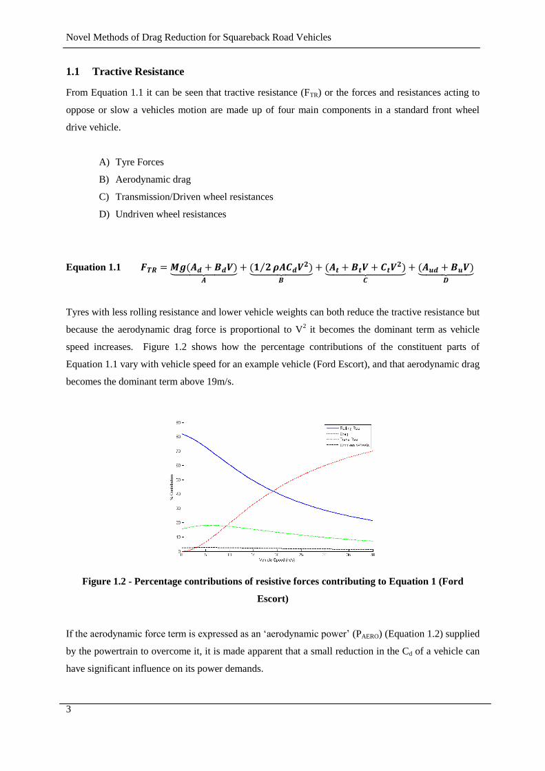
speed increases. Figure 1.2 shows how the percentage contributions of the constituent parts of
Equation 1.1 vary with vehicle speed for an example vehicle (Ford Escort), and that aerodynamic drag
becomes the dominant term above 19m/s.
Figure 1.2 - Percentage contributions of resistive forces contributing to Equation 1 (Ford
Escort)
If the aerodynamic force term is expressed as an ‘aerodynamic power’ (PAERO) (Equation 1.2) supplied
by the powertrain to overcome it, it is made apparent that a small reduction in the Cd of a vehicle can
have significant influence on its power demands.
Novel Methods of Drag Reduction for Squareback Road Vehicles
4
Equation 1.2
However, because aerodynamic power losses are also heavily dependent on vehicle speed their
influence on a calculated measure of vehicle fuel consumption becomes dependent on the drive cycle
used in the calculation. Some authors have suggested that if more realistic drive cycles were used
(relative to the current European drive cycles used) in calculations of CO2 contributions, it would
show that the influence of aerodynamic drag power is even more prominent than currently believed
(Schultz, 2010).
If engineers are to understand how Cd may be reduced it is important to understand what factors
influence the development of aerodynamic drag acting on a vehicle, and in the following sections
sources of drag for typical road car shapes will be investigated.
1.2 Sources of Drag
The aerodynamic drag force acting on a vehicle moving through air is a function of velocity (V),
vehicle frontal area (A) and Cd (Equation 1.3). Frontal area is generally determined by vehicle class,
component packaging, loading and ergonomic constraints, but has generally been increasing since the
1980’s. Cd can be manipulated by an aerodynamicist, in the pursuit of lower drag forces, but it must
be recognised that if frontal areas continue to increase any gains associated by lowering Cd will be
negated.
Equation 1.3
The resolved drag force along a vehicle body axis is the integration of the skin friction forces and the
normal pressure drag forces. Skin friction drag forces are the longitudinal component of viscous
forces created when air moves over the surfaces of a vehicle, and the pressure drag force is a result of
the fact that generally the pressure over rearward facing surfaces of a vehicle will be lower than the
forward facing ones. The pressure distribution around a vehicle body is influenced by a number of
factors such as; small scale separations, 3D separations or vortex formation, and shape configurations
that induce pressure gradients. In the case of a road vehicle skin friction drag is a relatively small
contributor (~15% (Hucho, 1998) (Ahmed, Ramm and Faltin, 1984)) to the overall drag force and
therefore the pressure drag is comparatively large. For that reason the work of the road vehicle
aerodynamicist will generally focus on creating a more favourable pressure distribution around the
vehicle body.
Novel Methods of Drag Reduction for Squareback Road Vehicles
5
Aerodynamic drag can also be broken down into its constituent parts in terms of it’s location of
generation (Carr, Atkin and Sommerville, 1994); forebody, afterbody, underbody, wheel and wheel
wells, protuberances, and engine cooling system. This breakdown was initially used to allow an
estimation of Cd and although this is not a very reliable technique, it assists in approximating the
relative contributions of each area to the total drag. In the current work it has been decided to focus
on the flow around the afterbody of the vehicle because around 40-60% (depending on vehicle shape)
of pressure drag is a result of the separations occurring in the afterbody area. Some of the main
contributors to drag in the afterbody region are low base pressures, trailing vortex generation, and
suction peaks on rearward facing surfaces.
1.2.1 Base Pressure and Vortex Drag
Base pressure drag is the result of low pressure flow in the wake of a vehicle generating low static
pressures on the rear facing surfaces. The overall size of the wake and magnitude of pressure within it
is largely determined by the vehicle shape, specifically the backlight configuration. The vehicle shape
causes variations in the velocity field such as separations which result in a failure to recover pressure.
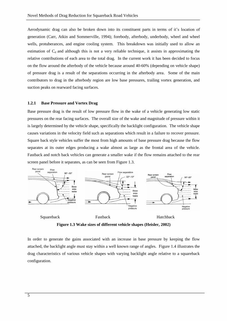
Square back style vehicles suffer the most from high amounts of base pressure drag because the flow
separates at its outer edges producing a wake almost as large as the frontal area of the vehicle.
Fastback and notch back vehicles can generate a smaller wake if the flow remains attached to the rear
screen panel before it separates, as can be seen from Figure 1.3.
Squareback Fastback Hatchback
Figure 1.3 Wake sizes of different vehicle shapes (Heisler, 2002)
In order to generate the gains associated with an increase in base pressure by keeping the flow
attached, the backlight angle must stay within a well known range of angles. Figure 1.4 illustrates the
drag characteristics of various vehicle shapes with varying backlight angle relative to a squareback
configuration.
Novel Methods of Drag Reduction for Squareback Road Vehicles
6
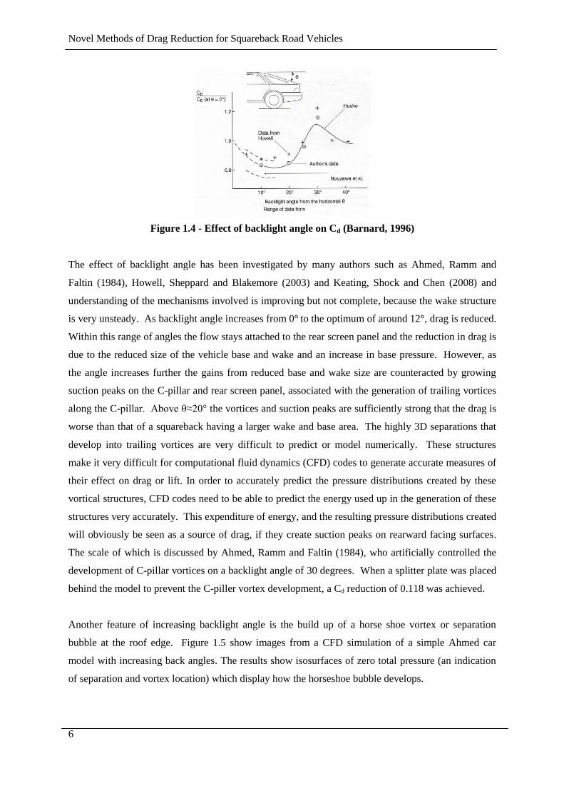
Figure 1.4 - Effect of backlight angle on Cd (Barnard, 1996)
The effect of backlight angle has been investigated by many authors such as Ahmed, Ramm and
Faltin (1984), Howell, Sheppard and Blakemore (2003) and Keating, Shock and Chen (2008) and
understanding of the mechanisms involved is improving but not complete, because the wake structure
is very unsteady. As backlight angle increases from 0° to the optimum of around 12°, drag is reduced.
Within this range of angles the flow stays attached to the rear screen panel and the reduction in drag is
due to the reduced size of the vehicle base and wake and an increase in base pressure. However, as
the angle increases further the gains from reduced base and wake size are counteracted by growing
suction peaks on the C-pillar and rear screen panel, associated with the generation of trailing vortices
along the C-pillar. Above θ≈20° the vortices and suction peaks are sufficiently strong that the drag is
worse than that of a squareback having a larger wake and base area. The highly 3D separations that
develop into trailing vortices are very difficult to predict or model numerically. These structures
make it very difficult for computational fluid dynamics (CFD) codes to generate accurate measures of
their effect on drag or lift. In order to accurately predict the pressure distributions created by these
vortical structures, CFD codes need to be able to predict the energy used up in the generation of these
structures very accurately. This expenditure of energy, and the resulting pressure distributions created
will obviously be seen as a source of drag, if they create suction peaks on rearward facing surfaces.
The scale of which is discussed by Ahmed, Ramm and Faltin (1984), who artificially controlled the
development of C-pillar vortices on a backlight angle of 30 degrees. When a splitter plate was placed
behind the model to prevent the C-piller vortex development, a Cd reduction of 0.118 was achieved.
Another feature of increasing backlight angle is the build up of a horse shoe vortex or separation
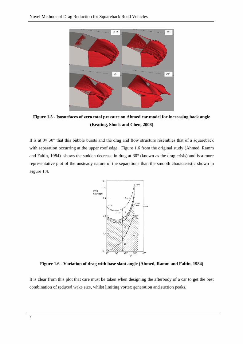
bubble at the roof edge. Figure 1.5 show images from a CFD simulation of a simple Ahmed car
model with increasing back angles. The results show isosurfaces of zero total pressure (an indication
of separation and vortex location) which display how the horseshoe bubble develops.
Novel Methods of Drag Reduction for Squareback Road Vehicles
7
Figure 1.5 - Isosurfaces of zero total pressure on Ahmed car model for increasing back angle
(Keating, Shock and Chen, 2008)
It is at θ≥ 30° that this bubble bursts and the drag and flow structure resembles that of a squareback
with separation occurring at the upper roof edge. Figure 1.6 from the original study (Ahmed, Ramm
and Faltin, 1984) shows the sudden decrease in drag at 30° (known as the drag crisis) and is a more
representative plot of the unsteady nature of the separations than the smooth characteristic shown in
Figure 1.4.
Figure 1.6 - Variation of drag with base slant angle (Ahmed, Ramm and Faltin, 1984)
It is clear from this plot that care must be taken when designing the afterbody of a car to get the best
combination of reduced wake size, whilst limiting vortex generation and suction peaks.
Novel Methods of Drag Reduction for Squareback Road Vehicles
8
1.2.2 Rear edge conditioning
Another technique used to try and reduce the wake area and increase the base pressure is address the
shape the rear separating edge to turn the flow in a desired way. If a radiused rear edge is used instead
of a sharp one, the magnitude and orientation of the radius can create positive or negative effects,
depending on the implementation
Although no plot for drag vs increasing rear edge radius has been found in previous automotive
aerodynamics work, previous publications such as Kee, Kim and Lee (2001) suggest that the variation
of Cd with increasing radius would be of a similar shape to Figure 1.6. As edge radius increases from
zero, Cd is expected to decrease to a minimum value at an optimum radius before rising to a worst
case value as suction around the radius increases and vortex strength increases. Whether or not a
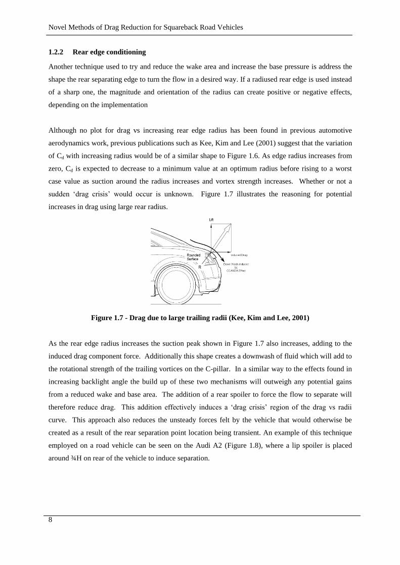
sudden ‘drag crisis’ would occur is unknown. Figure 1.7 illustrates the reasoning for potential
increases in drag using large rear radius.
Figure 1.7 - Drag due to large trailing radii (Kee, Kim and Lee, 2001)
As the rear edge radius increases the suction peak shown in Figure 1.7 also increases, adding to the
induced drag component force. Additionally this shape creates a downwash of fluid which will add to
the rotational strength of the trailing vortices on the C-pillar. In a similar way to the effects found in
increasing backlight angle the build up of these two mechanisms will outweigh any potential gains
from a reduced wake and base area. The addition of a rear spoiler to force the flow to separate will
therefore reduce drag. This addition effectively induces a ‘drag crisis’ region of the drag vs radii
curve. This approach also reduces the unsteady forces felt by the vehicle that would otherwise be
created as a result of the rear separation point location being transient. An example of this technique
employed on a road vehicle can be seen on the Audi A2 (Figure 1.8), where a lip spoiler is placed
around ¾H on rear of the vehicle to induce separation.

Novel Methods of Drag Reduction for Squareback Road Vehicles
9
Figure 1.8 - Audi A2 rear spoiler configuration
1.2.3 Drag Reduction Techniques
From the previous section the aims for reducing drag contributions of the afterbody section of a
vehicle can be summarised below:
Reduced wake and base size giving rise to increased static pressures on rearward facing
surfaces
Prevent the build up of trailing vortices whilst maintaining attachment of any rear slant
flow
Prevent the occurrence of suction peaks on rearward surfaces
Detail optimisation, and vehicle shape evolution have played a part in working towards these goals,
however an increasing number of investigations are being carried out into more novel passive and
active technologies to yield further gains.
1.3 Drag Reduction Techniques; Passive
1.3.1 Diffusers
Jowsey (2008) and Cooper et al. (1998) conducted studies on the performance of underbody diffusers
for drag and downforce production, both found that the performance is sensitive to ride height and
diffuser configuration. These studies suggest single channel underbody diffusers can offer drag
reductions at high ride heights and low diffuser angles, as can be seen from Figure 1.9 and Figure
1.10. At lower ride heights and higher diffuser angles ground effect and increased trailing vortex
strength increase downforce production, with the penalty of increased drag.
Novel Methods of Drag Reduction for Squareback Road Vehicles
10
Figure 1.9 – Drag produced by an underbody
diffuser at various angles and ride heights
(Cooper et al., 1998)
Figure 1.10 - Drag produced by an underbody
diffuser at various angles and ride heights
(Jowsey, 2008)
Figure 1.10 does not show tests on ride heights as high as Figure 1.9, however it is worthy of note that
the ride heights above 0.2h/H are unlikely to be found on any road vehicles. It should also be
highlighted that these configurations were tested on a fixed ground which may require a translation of
the curves in the y-axis if they are to be compared to a moving belt setup.
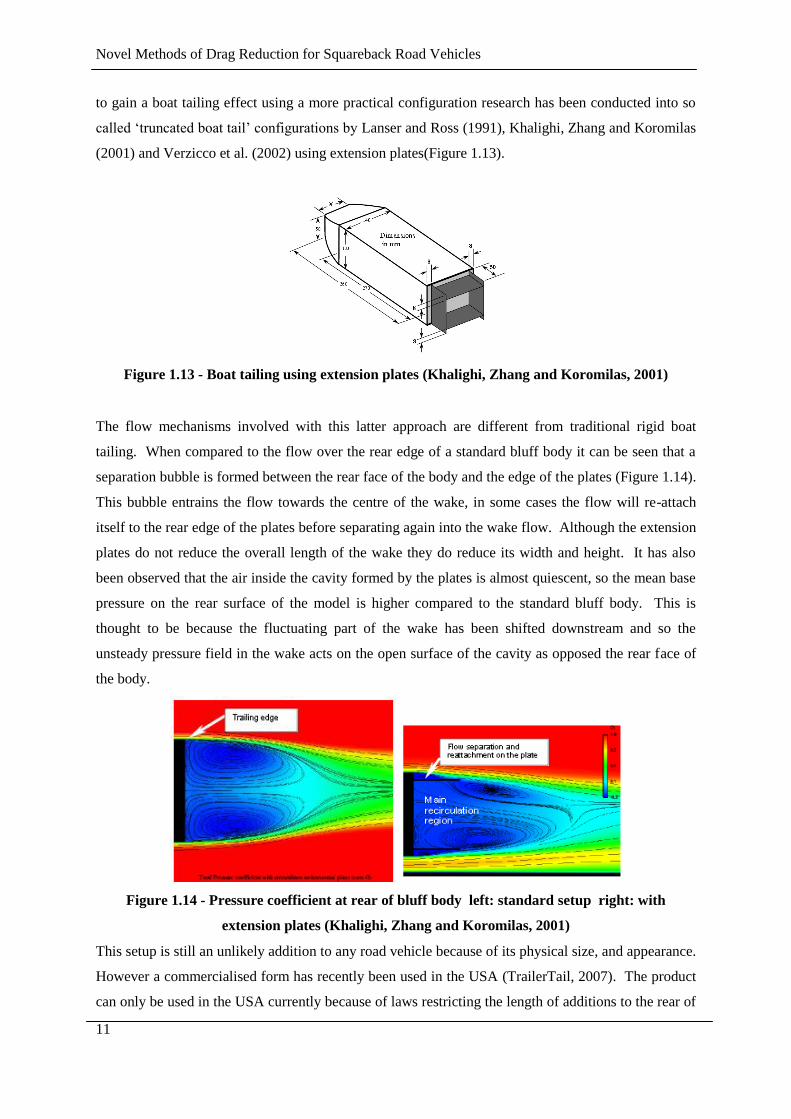
1.3.2 Boat Tailing
One of the oldest methods for reducing the size of a vehicles wake is known as boat tailing and would
prove most effective on squareback cars or lorries. In the process of boat tailing a bluff body or road
vehicle such as in Lanser and Ross (1991), Peterson (1981), Khalighi, Zhang and Koromilas (2001)
and Verzicco et al. (2002), the rear of the vehicle is modified as in Figure 1.11 and Figure 1.12 to
allow the flow to stay attached and so reduce size of the wake and the base pressure deficit. Wong and
Mair (1983) also showed that a ‘shortened boat tail’ such as in Figure 1.12 could be just as effective
as a ‘fully streamlined’ one in reducing drag.
Figure 1.11 - fully streamlined rigid boat tail
(Lanser and Ross, 1991)
Figure 1.12 - Shortened rigid boat tail fairing
(Wong and Mair, 1983)
Boat tailing takes its methodology from the basics of streamlining however the physical sizes and
shapes involved are the main limiting factor and are either impractical or even dangerous. In an effort
Novel Methods of Drag Reduction for Squareback Road Vehicles
11
to gain a boat tailing effect using a more practical configuration research has been conducted into so
called ‘truncated boat tail’ configurations by Lanser and Ross (1991), Khalighi, Zhang and Koromilas
(2001) and Verzicco et al. (2002) using extension plates(Figure 1.13).
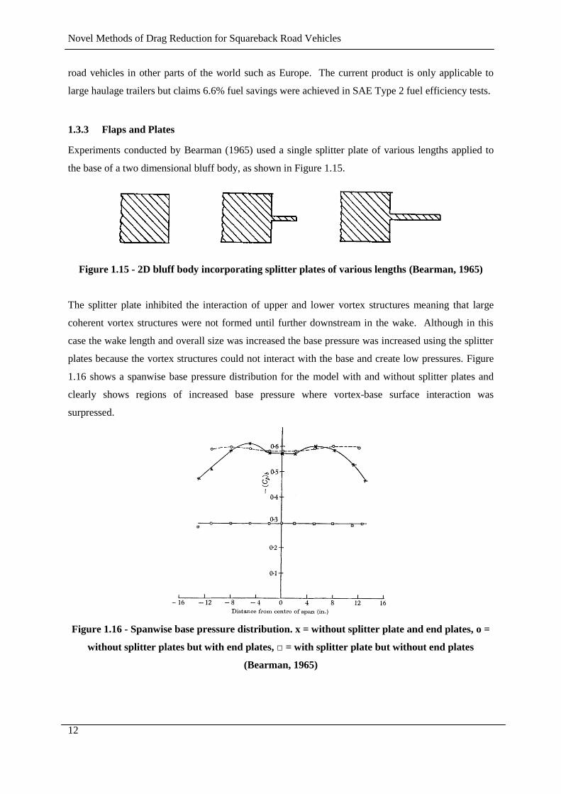
Figure 1.13 - Boat tailing using extension plates (Khalighi, Zhang and Koromilas, 2001)
The flow mechanisms involved with this latter approach are different from traditional rigid boat
tailing. When compared to the flow over the rear edge of a standard bluff body it can be seen that a
separation bubble is formed between the rear face of the body and the edge of the plates (Figure 1.14).
This bubble entrains the flow towards the centre of the wake, in some cases the flow will re-attach
itself to the rear edge of the plates before separating again into the wake flow. Although the extension
plates do not reduce the overall length of the wake they do reduce its width and height. It has also
been observed that the air inside the cavity formed by the plates is almost quiescent, so the mean base
pressure on the rear surface of the model is higher compared to the standard bluff body. This is
thought to be because the fluctuating part of the wake has been shifted downstream and so the
unsteady pressure field in the wake acts on the open surface of the cavity as opposed the rear face of
the body.
Figure 1.14 - Pressure coefficient at rear of bluff body left: standard setup right: with
extension plates (Khalighi, Zhang and Koromilas, 2001)
This setup is still an unlikely addition to any road vehicle because of its physical size, and appearance.
However a commercialised form has recently been used in the USA (TrailerTail, 2007). The product
can only be used in the USA currently because of laws restricting the length of additions to the rear of
Novel Methods of Drag Reduction for Squareback Road Vehicles
12
road vehicles in other parts of the world such as Europe. The current product is only applicable to
large haulage trailers but claims 6.6% fuel savings were achieved in SAE Type 2 fuel efficiency tests.
1.3.3 Flaps and Plates
Experiments conducted by Bearman (1965) used a single splitter plate of various lengths applied to
the base of a two dimensional bluff body, as shown in Figure 1.15.
Figure 1.15 - 2D bluff body incorporating splitter plates of various lengths (Bearman, 1965)
The splitter plate inhibited the interaction of upper and lower vortex structures meaning that large
coherent vortex structures were not formed until further downstream in the wake. Although in this
case the wake length and overall size was increased the base pressure was increased using the splitter
plates because the vortex structures could not interact with the base and create low pressures. Figure
1.16 shows a spanwise base pressure distribution for the model with and without splitter plates and
clearly shows regions of increased base pressure where vortex-base surface interaction was
surpressed.
Figure 1.16 - Spanwise base pressure distribution. x = without splitter plate and end plates, o =
without splitter plates but with end plates, □ = with splitter plate but without end plates
(Bearman, 1965)
Novel Methods of Drag Reduction for Squareback Road Vehicles
13
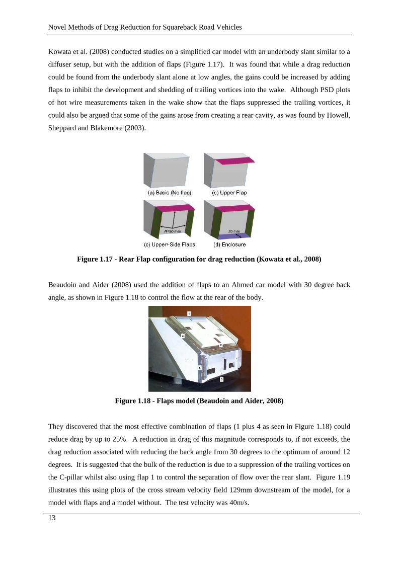
Kowata et al. (2008) conducted studies on a simplified car model with an underbody slant similar to a
diffuser setup, but with the addition of flaps (Figure 1.17). It was found that while a drag reduction
could be found from the underbody slant alone at low angles, the gains could be increased by adding
flaps to inhibit the development and shedding of trailing vortices into the wake. Although PSD plots
of hot wire measurements taken in the wake show that the flaps suppressed the trailing vortices, it
could also be argued that some of the gains arose from creating a rear cavity, as was found by Howell,
Sheppard and Blakemore (2003).
Figure 1.17 - Rear Flap configuration for drag reduction (Kowata et al., 2008)
Beaudoin and Aider (2008) used the addition of flaps to an Ahmed car model with 30 degree back
angle, as shown in Figure 1.18 to control the flow at the rear of the body.
Figure 1.18 - Flaps model (Beaudoin and Aider, 2008)
They discovered that the most effective combination of flaps (1 plus 4 as seen in Figure 1.18) could
reduce drag by up to 25%. A reduction in drag of this magnitude corresponds to, if not exceeds, the
drag reduction associated with reducing the back angle from 30 degrees to the optimum of around 12
degrees. It is suggested that the bulk of the reduction is due to a suppression of the trailing vortices on
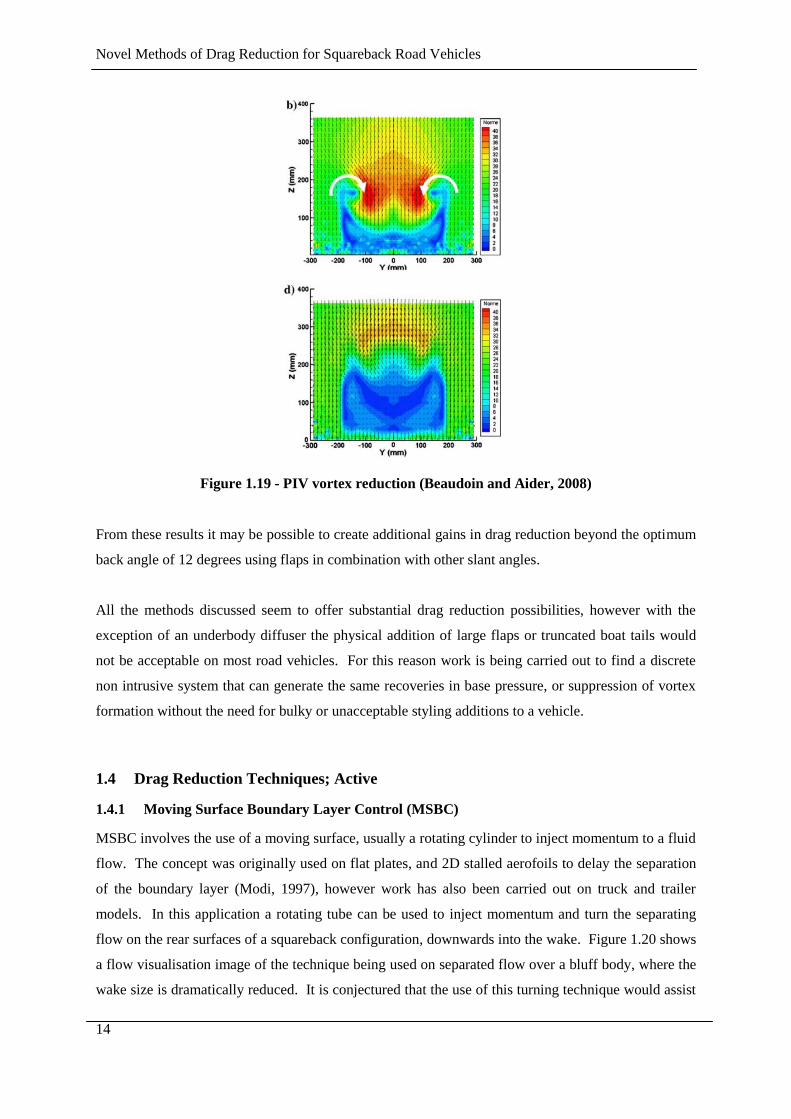
the C-pillar whilst also using flap 1 to control the separation of flow over the rear slant. Figure 1.19
illustrates this using plots of the cross stream velocity field 129mm downstream of the model, for a
model with flaps and a model without. The test velocity was 40m/s.
Novel Methods of Drag Reduction for Squareback Road Vehicles
14
Figure 1.19 - PIV vortex reduction (Beaudoin and Aider, 2008)
From these results it may be possible to create additional gains in drag reduction beyond the optimum
back angle of 12 degrees using flaps in combination with other slant angles.
All the methods discussed seem to offer substantial drag reduction possibilities, however with the
exception of an underbody diffuser the physical addition of large flaps or truncated boat tails would
not be acceptable on most road vehicles. For this reason work is being carried out to find a discrete
non intrusive system that can generate the same recoveries in base pressure, or suppression of vortex
formation without the need for bulky or unacceptable styling additions to a vehicle.
1.4 Drag Reduction Techniques; Active
1.4.1 Moving Surface Boundary Layer Control (MSBC)
MSBC involves the use of a moving surface, usually a rotating cylinder to inject momentum to a fluid
flow. The concept was originally used on flat plates, and 2D stalled aerofoils to delay the separation
of the boundary layer (Modi, 1997), however work has also been carried out on truck and trailer
models. In this application a rotating tube can be used to inject momentum and turn the separating
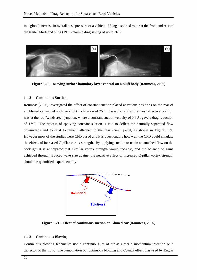
flow on the rear surfaces of a squareback configuration, downwards into the wake. Figure 1.20 shows
a flow visualisation image of the technique being used on separated flow over a bluff body, where the
wake size is dramatically reduced. It is conjectured that the use of this turning technique would assist
Novel Methods of Drag Reduction for Squareback Road Vehicles
15
in a global increase in overall base pressure of a vehicle. Using a splined roller at the front and rear of
the trailer Modi and Ying (1990) claim a drag saving of up to 26%
Figure 1.20 – Moving surface boundary layer control on a bluff body (Roumeas, 2006)
1.4.2 Continuous Suction
Roumeas (2006) investigated the effect of constant suction placed at various positions on the rear of
an Ahmed car model with backlight inclination of 25°. It was found that the most effective position
was at the roof/windscreen junction, where a constant suction velocity of 0.6U∞ gave a drag reduction
of 17%. The process of applying constant suction is said to deflect the naturally separated flow
downwards and force it to remain attached to the rear screen panel, as shown in Figure 1.21.
However most of the studies were CFD based and it is questionable how well the CFD could simulate
the effects of increased C-pillar vortex strength. By applying suction to retain an attached flow on the
backlight it is anticipated that C-pillar vortex strength would increase, and the balance of gains
achieved through reduced wake size against the negative effect of increased C-pillar vortex strength
should be quantified experimentally.
Figure 1.21 - Effect of continuous suction on Ahmed car (Roumeas, 2006)
1.4.3 Continuous Blowing
Continuous blowing techniques use a continuous jet of air as either a momentum injection or a
deflector of the flow. The combination of continuous blowing and Coanda effect was used by Englar
Novel Methods of Drag Reduction for Squareback Road Vehicles
16
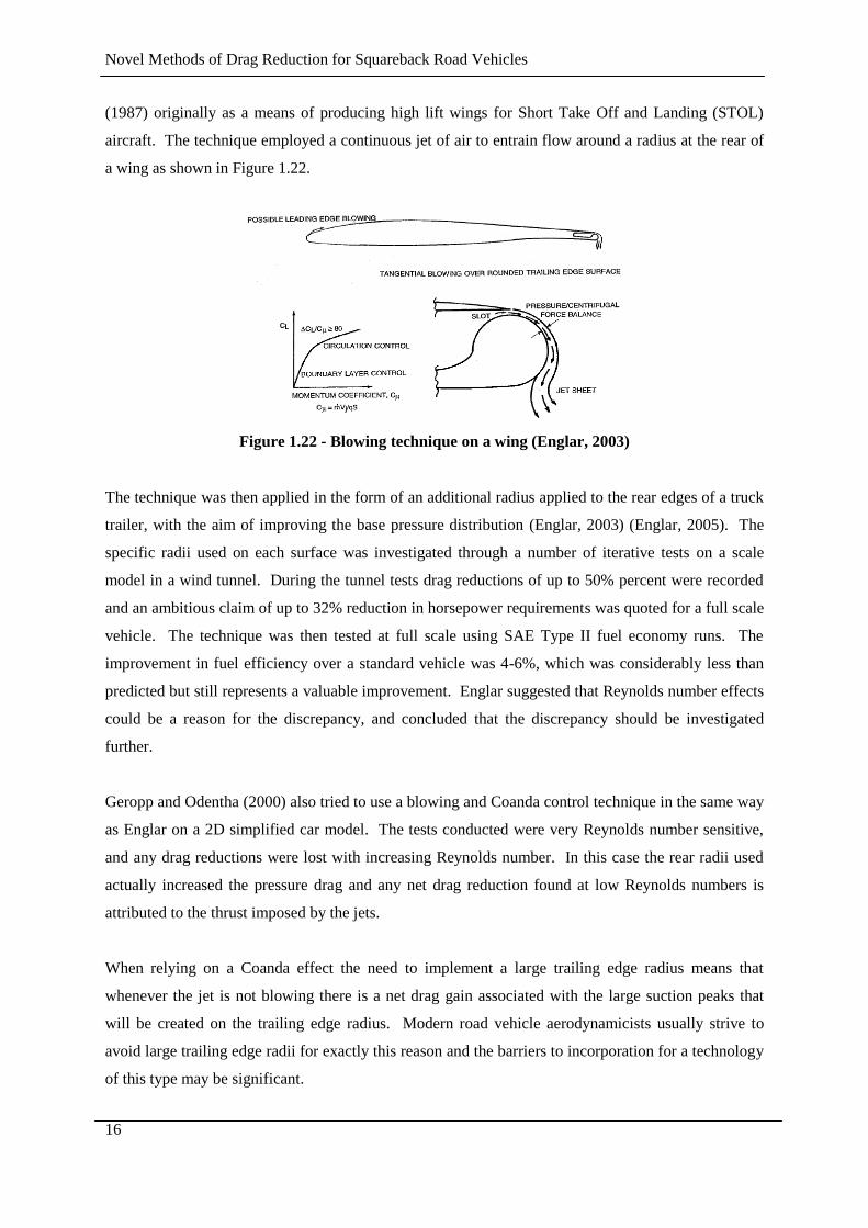
(1987) originally as a means of producing high lift wings for Short Take Off and Landing (STOL)
aircraft. The technique employed a continuous jet of air to entrain flow around a radius at the rear of
a wing as shown in Figure 1.22.
Figure 1.22 - Blowing technique on a wing (Englar, 2003)
The technique was then applied in the form of an additional radius applied to the rear edges of a truck
trailer, with the aim of improving the base pressure distribution (Englar, 2003) (Englar, 2005). The
specific radii used on each surface was investigated through a number of iterative tests on a scale
model in a wind tunnel. During the tunnel tests drag reductions of up to 50% percent were recorded
and an ambitious claim of up to 32% reduction in horsepower requirements was quoted for a full scale
vehicle. The technique was then tested at full scale using SAE Type II fuel economy runs. The
improvement in fuel efficiency over a standard vehicle was 4-6%, which was considerably less than
predicted but still represents a valuable improvement. Englar suggested that Reynolds number effects
could be a reason for the discrepancy, and concluded that the discrepancy should be investigated
further.
Geropp and Odentha (2000) also tried to use a blowing and Coanda control technique in the same way
as Englar on a 2D simplified car model. The tests conducted were very Reynolds number sensitive,
and any drag reductions were lost with increasing Reynolds number. In this case the rear radii used
actually increased the pressure drag and any net drag reduction found at low Reynolds numbers is
attributed to the thrust imposed by the jets.
When relying on a Coanda effect the need to implement a large trailing edge radius means that
whenever the jet is not blowing there is a net drag gain associated with the large suction peaks that
will be created on the trailing edge radius. Modern road vehicle aerodynamicists usually strive to
avoid large trailing edge radii for exactly this reason and the barriers to incorporation for a technology
of this type may be significant.
Novel Methods of Drag Reduction for Squareback Road Vehicles
17
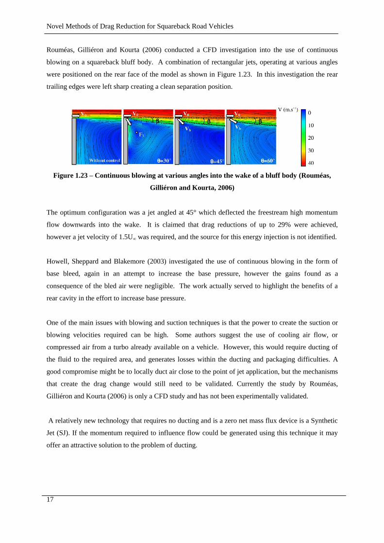
Rouméas, Gilliéron and Kourta (2006) conducted a CFD investigation into the use of continuous
blowing on a squareback bluff body. A combination of rectangular jets, operating at various angles
were positioned on the rear face of the model as shown in Figure 1.23. In this investigation the rear
trailing edges were left sharp creating a clean separation position.
Figure 1.23 – Continuous blowing at various angles into the wake of a bluff body (Rouméas,
Gilliéron and Kourta, 2006)
The optimum configuration was a jet angled at 45° which deflected the freestream high momentum
flow downwards into the wake. It is claimed that drag reductions of up to 29% were achieved,
however a jet velocity of 1.5U∞ was required, and the source for this energy injection is not identified.
Howell, Sheppard and Blakemore (2003) investigated the use of continuous blowing in the form of
base bleed, again in an attempt to increase the base pressure, however the gains found as a
consequence of the bled air were negligible. The work actually served to highlight the benefits of a
rear cavity in the effort to increase base pressure.
One of the main issues with blowing and suction techniques is that the power to create the suction or
blowing velocities required can be high. Some authors suggest the use of cooling air flow, or
compressed air from a turbo already available on a vehicle. However, this would require ducting of
the fluid to the required area, and generates losses within the ducting and packaging difficulties. A
good compromise might be to locally duct air close to the point of jet application, but the mechanisms
that create the drag change would still need to be validated. Currently the study by Rouméas,
Gilliéron and Kourta (2006) is only a CFD study and has not been experimentally validated.
A relatively new technology that requires no ducting and is a zero net mass flux device is a Synthetic
Jet (SJ). If the momentum required to influence flow could be generated using this technique it may
offer an attractive solution to the problem of ducting.
Novel Methods of Drag Reduction for Squareback Road Vehicles
18
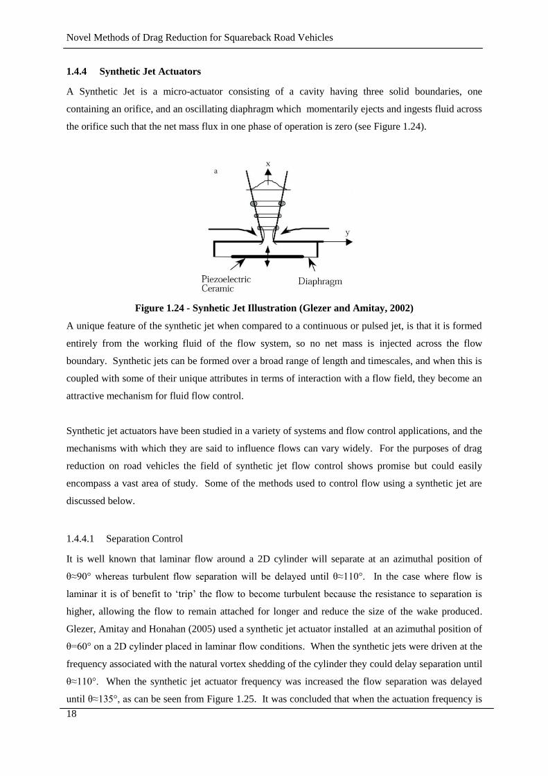
1.4.4 Synthetic Jet Actuators
A Synthetic Jet is a micro-actuator consisting of a cavity having three solid boundaries, one
containing an orifice, and an oscillating diaphragm which momentarily ejects and ingests fluid across
the orifice such that the net mass flux in one phase of operation is zero (see Figure 1.24).
Figure 1.24 - Synhetic Jet Illustration (Glezer and Amitay, 2002)
A unique feature of the synthetic jet when compared to a continuous or pulsed jet, is that it is formed
entirely from the working fluid of the flow system, so no net mass is injected across the flow
boundary. Synthetic jets can be formed over a broad range of length and timescales, and when this is
coupled with some of their unique attributes in terms of interaction with a flow field, they become an
attractive mechanism for fluid flow control.
Synthetic jet actuators have been studied in a variety of systems and flow control applications, and the
mechanisms with which they are said to influence flows can vary widely. For the purposes of drag
reduction on road vehicles the field of synthetic jet flow control shows promise but could easily
encompass a vast area of study. Some of the methods used to control flow using a synthetic jet are
discussed below.
1.4.4.1 Separation Control
It is well known that laminar flow around a 2D cylinder will separate at an azimuthal position of
θ≈90° whereas turbulent flow separation will be delayed until θ≈110°. In the case where flow is
laminar it is of benefit to ‘trip’ the flow to become turbulent because the resistance to separation is
higher, allowing the flow to remain attached for longer and reduce the size of the wake produced.
Glezer, Amitay and Honahan (2005) used a synthetic jet actuator installed at an azimuthal position of
θ=60° on a 2D cylinder placed in laminar flow conditions. When the synthetic jets were driven at the
frequency associated with the natural vortex shedding of the cylinder they could delay separation until
θ≈110°. When the synthetic jet actuator frequency was increased the flow separation was delayed
until θ≈135°, as can be seen from Figure 1.25. It was concluded that when the actuation frequency is

Novel Methods of Drag Reduction for Squareback Road Vehicles
19
nominally of the same order as the natural shedding frequency (or up to five times magnitude) the
performance of the actuator in influencing the point of separation increases with increasing actuation
frequency. At actuation frequencies above five times the natural shedding frequency, performance
becomes invariant with actuation frequency. Unfortunately in road vehicle applications the flow is
usually turbulent and any gains found in laminar flow may be lost when introduced in a turbulent
flow.
Figure 1.25 - Variation of the pressure coefficient around a tube with increasing dimensionless
actuation frequency SrD act = •;0.24, Δ;0.50, *; 0.83 and -; base line flow (Glezer, Amitay and
Honahan, 2005)
Glezer, Amitay and Honahan (2005) and Béra et al. (2000) investigated this effect using conventional
trip wires on the front of the cylinder to create a turbulent boundary layer. The synthetic jet was
oriented at an azimuthal position of 110° relative to the freestream direction. Pressure distributions
around the tube studied by Glezer, Amitay and Honahan (2005) (Figure 1.26) and by Béra et al.
(2000) (Figure 1.27) are shown below.
Novel Methods of Drag Reduction for Squareback Road Vehicles
20
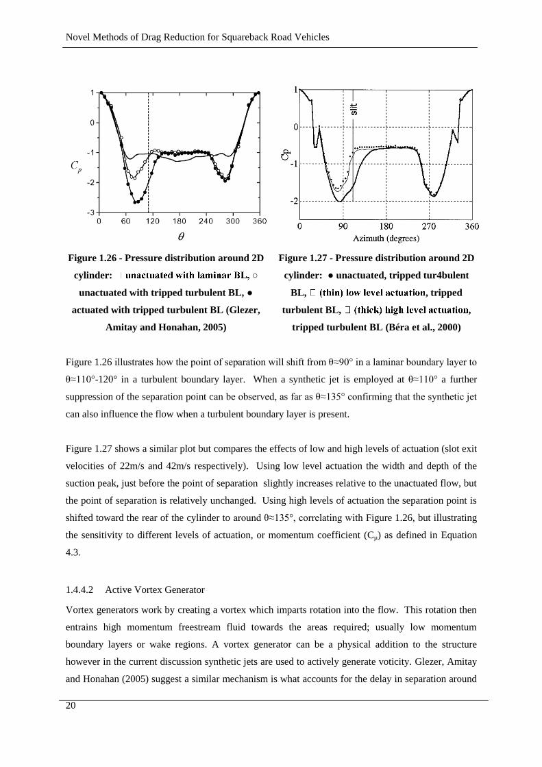
Figure 1.26 - Pressure distribution around 2D
cylinder: ○
unactuated with tripped turbulent BL, ●
actuated with tripped turbulent BL (Glezer,
Amitay and Honahan, 2005)
Figure 1.27 - Pressure distribution around 2D
cylinder: ● unactuated, tripped tur4bulent
BL, , tripped
turbulent BL, ,
tripped turbulent BL (Béra et al., 2000)
Figure 1.26 illustrates how the point of separation will shift from θ≈90° in a laminar boundary layer to
θ≈110°-120° in a turbulent boundary layer. When a synthetic jet is employed at θ≈110° a further
suppression of the separation point can be observed, as far as θ≈135° confirming that the synthetic jet
can also influence the flow when a turbulent boundary layer is present.
Figure 1.27 shows a similar plot but compares the effects of low and high levels of actuation (slot exit
velocities of 22m/s and 42m/s respectively). Using low level actuation the width and depth of the
suction peak, just before the point of separation slightly increases relative to the unactuated flow, but
the point of separation is relatively unchanged. Using high levels of actuation the separation point is
shifted toward the rear of the cylinder to around θ≈135°, correlating with Figure 1.26, but illustrating
the sensitivity to different levels of actuation, or momentum coefficient (Cµ) as defined in Equation
4.3.
1.4.4.2 Active Vortex Generator
Vortex generators work by creating a vortex which imparts rotation into the flow. This rotation then
entrains high momentum freestream fluid towards the areas required; usually low momentum
boundary layers or wake regions. A vortex generator can be a physical addition to the structure
however in the current discussion synthetic jets are used to actively generate voticity. Glezer, Amitay
and Honahan (2005) suggest a similar mechanism is what accounts for the delay in separation around
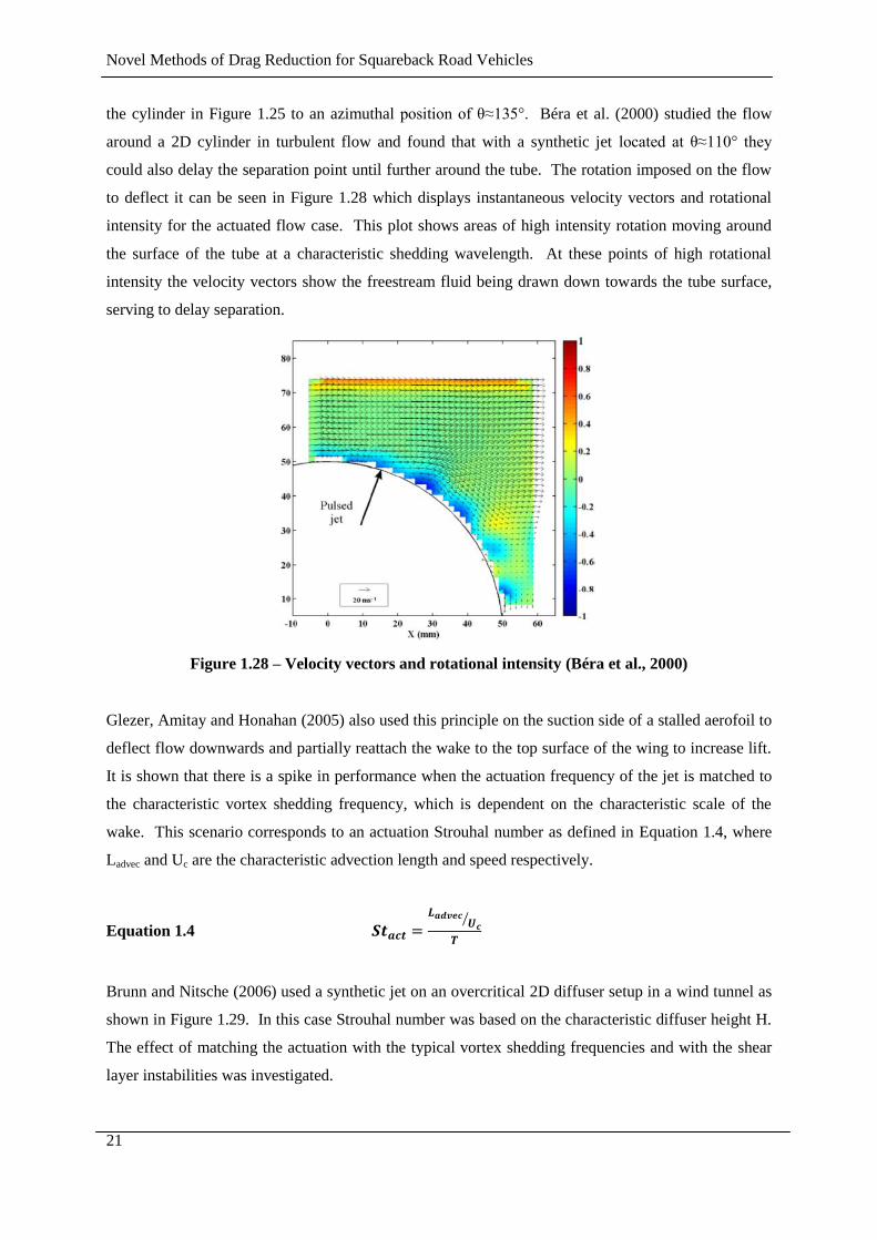
Novel Methods of Drag Reduction for Squareback Road Vehicles
21
the cylinder in Figure 1.25 to an azimuthal position of θ≈135°. Béra et al. (2000) studied the flow
around a 2D cylinder in turbulent flow and found that with a synthetic jet located at θ≈110° they
could also delay the separation point until further around the tube. The rotation imposed on the flow
to deflect it can be seen in Figure 1.28 which displays instantaneous velocity vectors and rotational
intensity for the actuated flow case. This plot shows areas of high intensity rotation moving around
the surface of the tube at a characteristic shedding wavelength. At these points of high rotational
intensity the velocity vectors show the freestream fluid being drawn down towards the tube surface,
serving to delay separation.
Figure 1.28 – Velocity vectors and rotational intensity (Béra et al., 2000)
Glezer, Amitay and Honahan (2005) also used this principle on the suction side of a stalled aerofoil to
deflect flow downwards and partially reattach the wake to the top surface of the wing to increase lift.
It is shown that there is a spike in performance when the actuation frequency of the jet is matched to
the characteristic vortex shedding frequency, which is dependent on the characteristic scale of the
wake. This scenario corresponds to an actuation Strouhal number as defined in Equation 1.4, where
Ladvec and Uc are the characteristic advection length and speed respectively.
Equation 1.4
Brunn and Nitsche (2006) used a synthetic jet on an overcritical 2D diffuser setup in a wind tunnel as
shown in Figure 1.29. In this case Strouhal number was based on the characteristic diffuser height H.
The effect of matching the actuation with the typical vortex shedding frequencies and with the shear
layer instabilities was investigated.
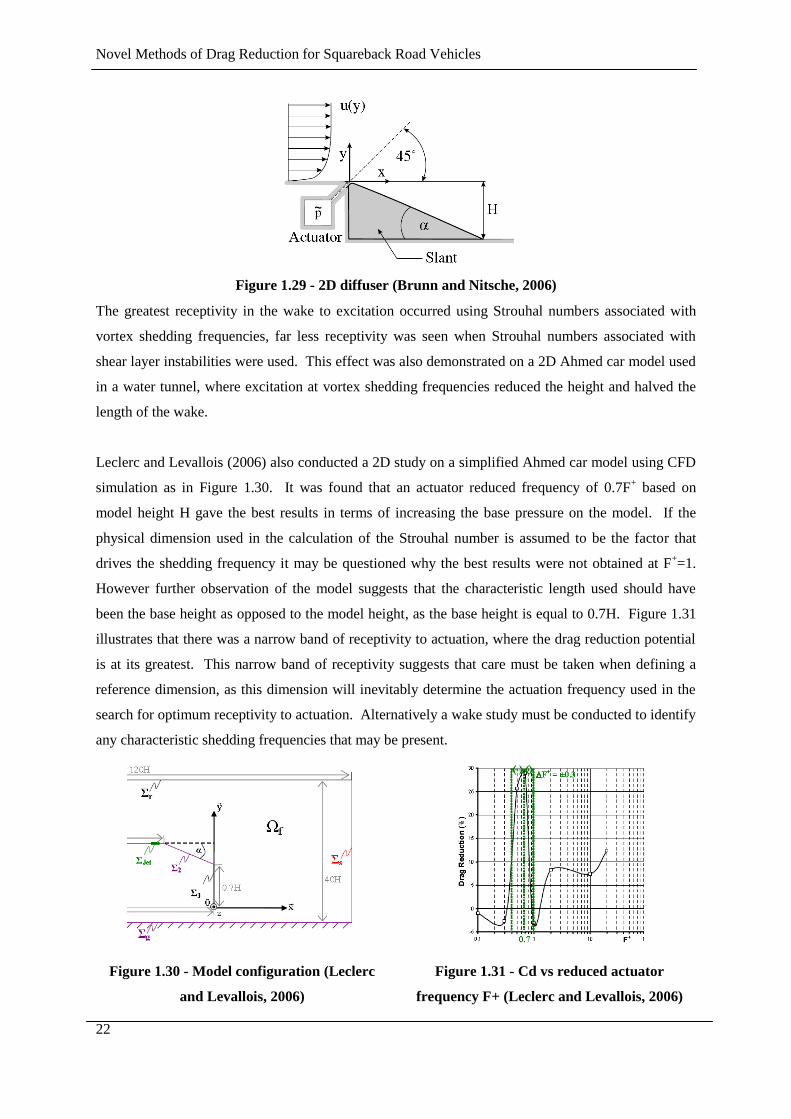
Novel Methods of Drag Reduction for Squareback Road Vehicles
22
Figure 1.29 - 2D diffuser (Brunn and Nitsche, 2006)
The greatest receptivity in the wake to excitation occurred using Strouhal numbers associated with
vortex shedding frequencies, far less receptivity was seen when Strouhal numbers associated with
shear layer instabilities were used. This effect was also demonstrated on a 2D Ahmed car model used
in a water tunnel, where excitation at vortex shedding frequencies reduced the height and halved the
length of the wake.
Leclerc and Levallois (2006) also conducted a 2D study on a simplified Ahmed car model using CFD
simulation as in Figure 1.30. It was found that an actuator reduced frequency of 0.7F+ based on
model height H gave the best results in terms of increasing the base pressure on the model. If the
physical dimension used in the calculation of the Strouhal number is assumed to be the factor that
drives the shedding frequency it may be questioned why the best results were not obtained at F+=1.
However further observation of the model suggests that the characteristic length used should have
been the base height as opposed to the model height, as the base height is equal to 0.7H. Figure 1.31
illustrates that there was a narrow band of receptivity to actuation, where the drag reduction potential
is at its greatest. This narrow band of receptivity suggests that care must be taken when defining a
reference dimension, as this dimension will inevitably determine the actuation frequency used in the
search for optimum receptivity to actuation. Alternatively a wake study must be conducted to identify
any characteristic shedding frequencies that may be present.
Figure 1.30 - Model configuration (Leclerc
and Levallois, 2006)
Figure 1.31 - Cd vs reduced actuator
frequency F+ (Leclerc and Levallois, 2006)
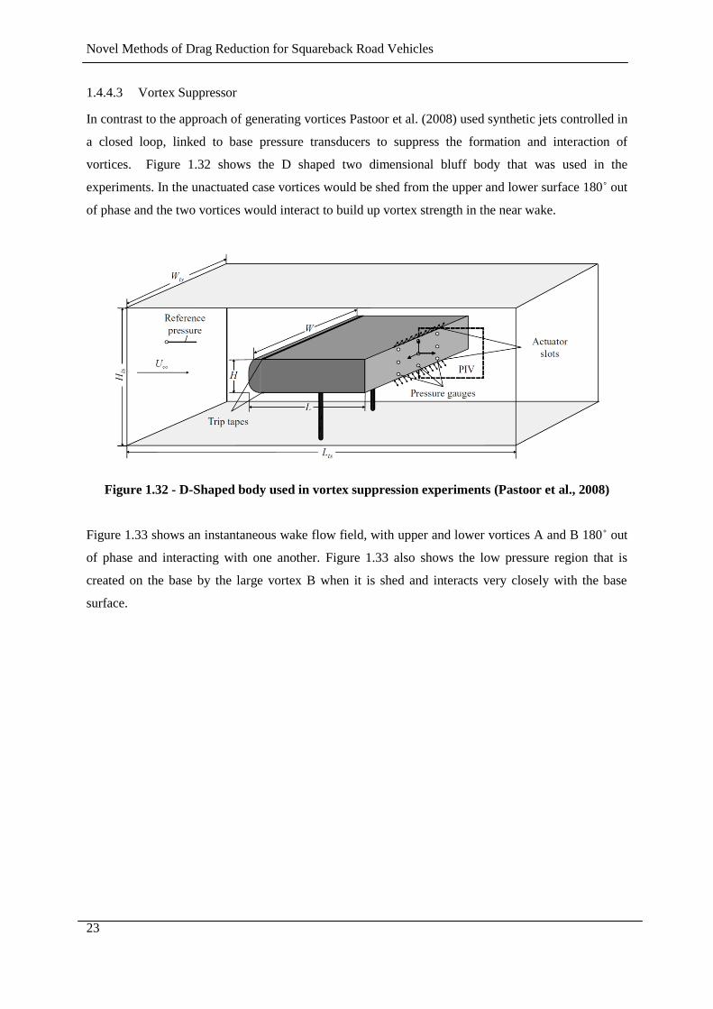
Novel Methods of Drag Reduction for Squareback Road Vehicles
23
1.4.4.3 Vortex Suppressor
In contrast to the approach of generating vortices Pastoor et al. (2008) used synthetic jets controlled in
a closed loop, linked to base pressure transducers to suppress the formation and interaction of
vortices. Figure 1.32 shows the D shaped two dimensional bluff body that was used in the
experiments. In the unactuated case vortices would be shed from the upper and lower surface 180˚ out
of phase and the two vortices would interact to build up vortex strength in the near wake.
Figure 1.32 - D-Shaped body used in vortex suppression experiments (Pastoor et al., 2008)
Figure 1.33 shows an instantaneous wake flow field, with upper and lower vortices A and B 180˚ out
of phase and interacting with one another. Figure 1.33 also shows the low pressure region that is
created on the base by the large vortex B when it is shed and interacts very closely with the base
surface.
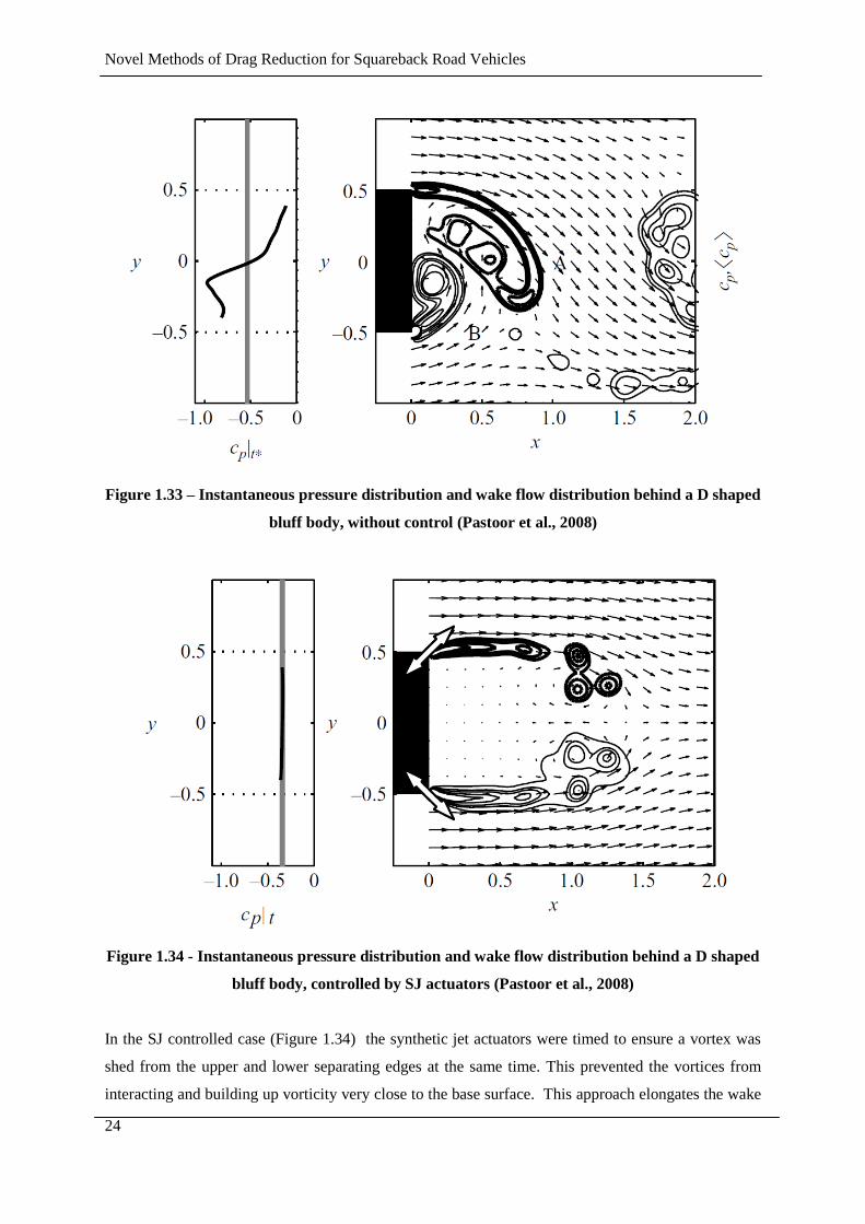
Novel Methods of Drag Reduction for Squareback Road Vehicles
24
Figure 1.33 – Instantaneous pressure distribution and wake flow distribution behind a D shaped
bluff body, without control (Pastoor et al., 2008)
Figure 1.34 - Instantaneous pressure distribution and wake flow distribution behind a D shaped
bluff body, controlled by SJ actuators (Pastoor et al., 2008)
In the SJ controlled case (Figure 1.34) the synthetic jet actuators were timed to ensure a vortex was
shed from the upper and lower separating edges at the same time. This prevented the vortices from
interacting and building up vorticity very close to the base surface. This approach elongates the wake
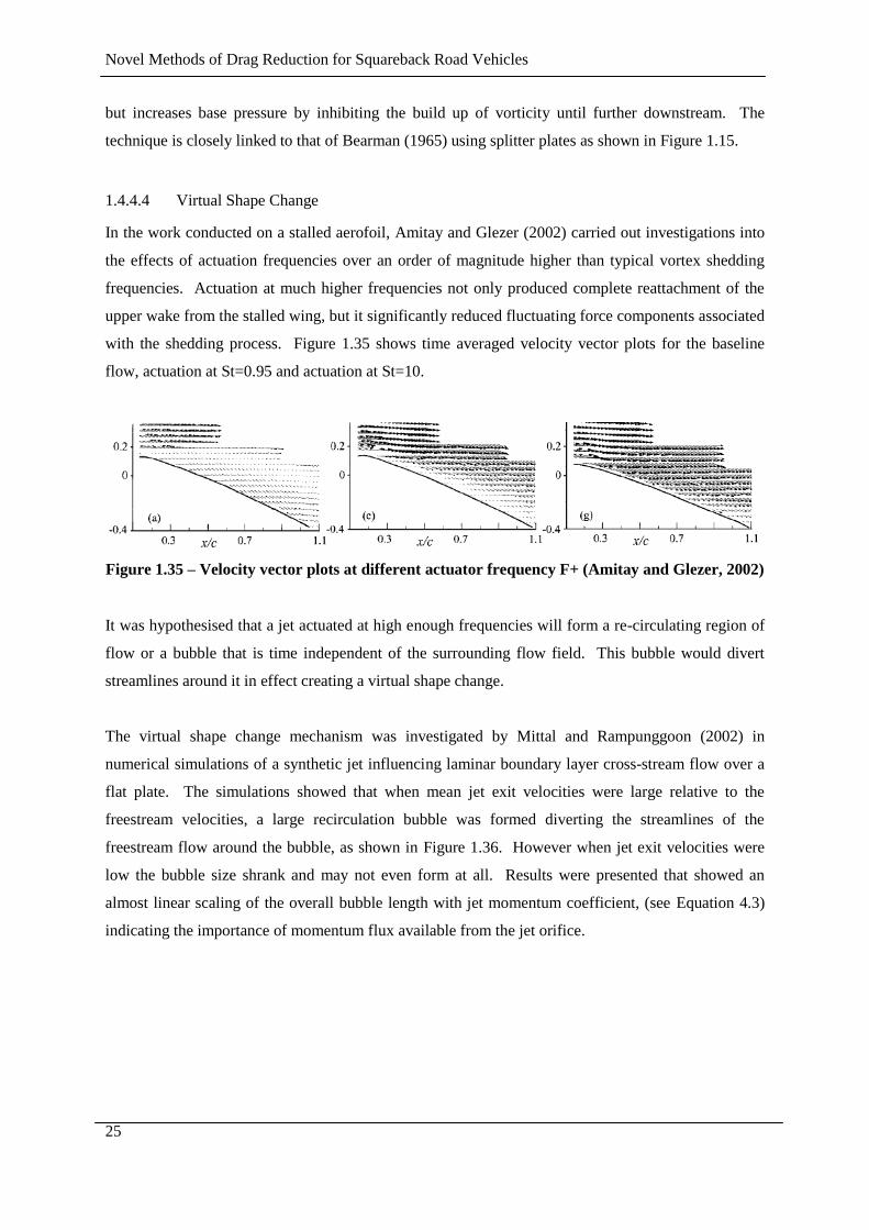
Novel Methods of Drag Reduction for Squareback Road Vehicles
25
but increases base pressure by inhibiting the build up of vorticity until further downstream. The
technique is closely linked to that of Bearman (1965) using splitter plates as shown in Figure 1.15.
1.4.4.4 Virtual Shape Change
In the work conducted on a stalled aerofoil, Amitay and Glezer (2002) carried out investigations into
the effects of actuation frequencies over an order of magnitude higher than typical vortex shedding
frequencies. Actuation at much higher frequencies not only produced complete reattachment of the
upper wake from the stalled wing, but it significantly reduced fluctuating force components associated
with the shedding process. Figure 1.35 shows time averaged velocity vector plots for the baseline
flow, actuation at St=0.95 and actuation at St=10.
Figure 1.35 – Velocity vector plots at different actuator frequency F+ (Amitay and Glezer, 2002)
It was hypothesised that a jet actuated at high enough frequencies will form a re-circulating region of
flow or a bubble that is time independent of the surrounding flow field. This bubble would divert
streamlines around it in effect creating a virtual shape change.
The virtual shape change mechanism was investigated by Mittal and Rampunggoon (2002) in
numerical simulations of a synthetic jet influencing laminar boundary layer cross-stream flow over a
flat plate. The simulations showed that when mean jet exit velocities were large relative to the
freestream velocities, a large recirculation bubble was formed diverting the streamlines of the
freestream flow around the bubble, as shown in Figure 1.36. However when jet exit velocities were
low the bubble size shrank and may not even form at all. Results were presented that showed an
almost linear scaling of the overall bubble length with jet momentum coefficient, (see Equation 4.3)
indicating the importance of momentum flux available from the jet orifice.
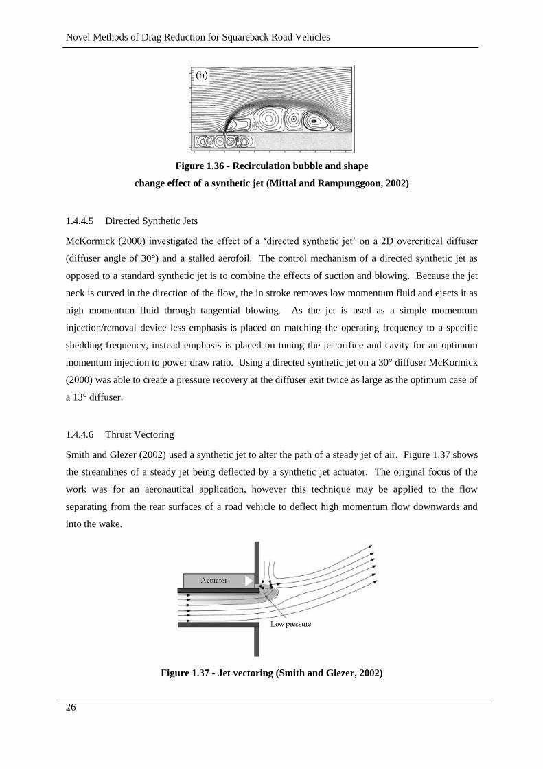
Novel Methods of Drag Reduction for Squareback Road Vehicles
26
Figure 1.36 - Recirculation bubble and shape
change effect of a synthetic jet (Mittal and Rampunggoon, 2002)
1.4.4.5 Directed Synthetic Jets
McKormick (2000) investigated the effect of a ‘directed synthetic jet’ on a 2D overcritical diffuser
(diffuser angle of 30°) and a stalled aerofoil. The control mechanism of a directed synthetic jet as
opposed to a standard synthetic jet is to combine the effects of suction and blowing. Because the jet
neck is curved in the direction of the flow, the in stroke removes low momentum fluid and ejects it as
high momentum fluid through tangential blowing. As the jet is used as a simple momentum
injection/removal device less emphasis is placed on matching the operating frequency to a specific
shedding frequency, instead emphasis is placed on tuning the jet orifice and cavity for an optimum
momentum injection to power draw ratio. Using a directed synthetic jet on a 30° diffuser McKormick
(2000) was able to create a pressure recovery at the diffuser exit twice as large as the optimum case of
a 13° diffuser.
1.4.4.6 Thrust Vectoring
Smith and Glezer (2002) used a synthetic jet to alter the path of a steady jet of air. Figure 1.37 shows
the streamlines of a steady jet being deflected by a synthetic jet actuator. The original focus of the
work was for an aeronautical application, however this technique may be applied to the flow
separating from the rear surfaces of a road vehicle to deflect high momentum flow downwards and
into the wake.
Figure 1.37 - Jet vectoring (Smith and Glezer, 2002)
Novel Methods of Drag Reduction for Squareback Road Vehicles
27
1.5 Drag Reduction Techniques; Further Investigation
From the work discussed above some of the least intrusive techniques that show the greatest potential
for drag reduction are constant blowing and suction, pulsed blowing and suction, and synthetic jets.
The apparent low power and weight demands of the synthetic jet actuator as a means of flow control
makes it stand out as an area to investigate further for road vehicle applications.
The different modes of operation and control open a wide scope for research work; in the work
reported here the focus is on vehicle afterbody flow regimes. This work will study the use of
blowing, pulsed blowing and synthetic jets to control flow separations from the rear upper roof edge
of a vehicle. The modes of use of blowing or a synthetic jet located at this position to be investigated
include; thrust vectoring, directed synthetic jets, virtual shape change devices, active vortex
generators and vortex suppression.
It is also recognised that synthetic jet flow control techniques could prove useful in controlling
separations in other locations on a vehicle such as, A-pillars, C-pillars, wheel arches, front edge radii,
sunroofs and diffusers. The upper roof edge was chosen for investigation because it is an area where
the flow structures will be least three dimensional, especially at and around the model centreline. The
majority of previous work using SJ actuators has been conducted using 2D configurations such as
wings and cylinders, and so it was decided to avoid attempts to control 3D structures as far as is
possible on automotive bluff bodies. However, before an active control technique can be used to
control the flow around a vehicle it is important that the flow structures intended to be controlled are
understood as fully as possible.
The main objectives for the thesis include:
Identify flow regimes in the wake of square back vehicles which can be targeted
using active flow control
Design and develop actuators and means of creating active flow control devices, such
as synthetic jets, pulsed jets or blowing
Apply the actuators to a 3D bluff body configuration representative of a squareback
vehicle model in an attempt to control the wake flow and reduce drag
Conduct tests at appropriately large freestream Reynolds numbers that could be
considered to be matched with full scale configurations
Identify the mechanisms which contribute to changes in drag and lift as a result of the
applied actuation method

Novel Methods of Drag Reduction for Squareback Road Vehicles
28
In order to satisfy the objectives, tests are conducted in the Loughborough University ¼ scale wind
tunnel using a number of different data acquisition techniques. These techniques are discussed in
Chapter 2 followed by an experimental investigation into the flow structures behind a simplified
squareback vehicle model which is discussed in Chapter 3.
Novel Methods of Drag Reduction for Squareback Road Vehicles
29
Chapter 2
EXPERIMENTAL METHOD
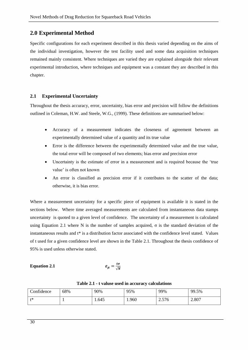
Novel Methods of Drag Reduction for Squareback Road Vehicles
30
2.0 Experimental Method
Specific configurations for each experiment described in this thesis varied depending on the aims of
the individual investigation, however the test facility used and some data acquisition techniques
remained mainly consistent. Where techniques are varied they are explained alongside their relevant
experimental introduction, where techniques and equipment was a constant they are described in this
chapter.
2.1 Experimental Uncertainty
Throughout the thesis accuracy, error, uncertainty, bias error and precision will follow the definitions
outlined in Coleman, H.W. and Steele, W.G., (1999). These definitions are summarised below:
Accuracy of a measurement indicates the closeness of agreement between an
experimentally determined value of a quantity and its true value
Error is the difference between the experimentally determined value and the true value,
the total error will be composed of two elements; bias error and precision error
Uncertainty is the estimate of error in a measurement and is required because the ‘true
value’ is often not known
An error is classified as precision error if it contributes to the scatter of the data;
otherwise, it is bias error.
Where a measurement uncertainty for a specific piece of equipment is available it is stated in the
sections below. Where time averaged measurements are calculated from instantaneous data stamps
uncertainty is quoted to a given level of confidence. The uncertainty of a measurement is calculated
using Equation 2.1 where N is the number of samples acquired, σ is the standard deviation of the
instantaneous results and t* is a distribution factor associated with the confidence level stated. Values
of t used for a given confidence level are shown in the Table 2.1. Throughout the thesis confidence of
95% is used unless otherwise stated.
Equation 2.1
Table 2.1 - t valuse used in accuracy calculations
Confidence 68% 90% 95% 99% 99.5%
t* 1 1.645 1.960 2.576 2.807

Novel Methods of Drag Reduction for Squareback Road Vehicles
31
2.2 Wind Tunnel and Force Balance
All tests were conducted in the Loughborough University closed working section, open circuit wind
tunnel (Figure 2.1). The working section of the tunnel is 1.92mx1.32m and it is capable of operating
between speeds of 5-45m/s. At test speeds of 40m/s the freestream turbulence intensity is less than
0.2% and the boundary layer is typically 50-60mm thick at the model centreline position. Tunnel
velocity is calculated from measurements of tunnel air temperature, ambient pressure, and freestream
total and static pressure.
Figure 2.1 - Loughborough University Wind Tunnel
The pitot tube is mounted from the roof of the working section 2m upstream of the model centreline
position. Total and static pressures are recorded via a Furness Controls FC0332 differential pressure
transducer accurate to ±2.5mmH2O of the full range of ±250mmH2O. Temperature is recorded using
a thermocouple mounted inside a pitot tube and ambient pressure is measured using a barometer
located in the wind tunnel control room.
The tunnel is equipped with a six component under floor balance capable of logging force data at
speeds of up to 250Hz. The high acquisition speeds can be used to perform temporal analysis of the
aerodynamic forces applied to a model, however within this thesis data is acquired at 5Hz and
averaged over a 30 second sampling time. However the data stamps taken at 5Hz are themselves
block averaged from a raw voltage signal running at 4.6KHz. Once the balance has been calibrated
data in each axis is accurate to the values shown in Table 2.2.
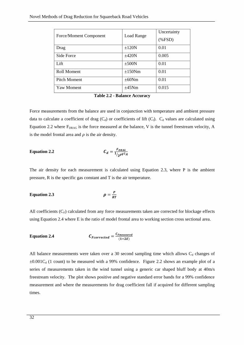
Novel Methods of Drag Reduction for Squareback Road Vehicles
32
Force/Moment Component Load Range Uncertainty
(%FSD)
Drag ±120N 0.01
Side Force ±420N 0.005
Lift ±500N 0.01
Roll Moment ±150Nm 0.01
Pitch Moment ±60Nm 0.01
Yaw Moment ±45Nm 0.015
Table 2.2 - Balance Accuracy
Force measurements from the balance are used in conjunction with temperature and ambient pressure
data to calculate a coefficient of drag (Cd) or coefficients of lift (Cl). Cd values are calculated using
Equation 2.2 where FDRAG is the force measured at the balance, V is the tunnel freestream velocity, A
is the model frontal area and is the air density.
Equation 2.2
The air density for each measurement is calculated using Equation 2.3, where P is the ambient
pressure, R is the specific gas constant and T is the air temperature.
Equation 2.3
All coefficients (CF) calculated from any force measurements taken are corrected for blockage effects
using Equation 2.4 where E is the ratio of model frontal area to working section cross sectional area.
Equation 2.4
All balance measurements were taken over a 30 second sampling time which allows Cd changes of
±0.001Cd (1 count) to be measured with a 99% confidence. Figure 2.2 shows an example plot of a
series of measurements taken in the wind tunnel using a generic car shaped bluff body at 40m/s
freestream velocity. The plot shows positive and negative standard error bands for a 99% confidence
measurement and where the measurements for drag coefficient fall if acquired for different sampling
times.
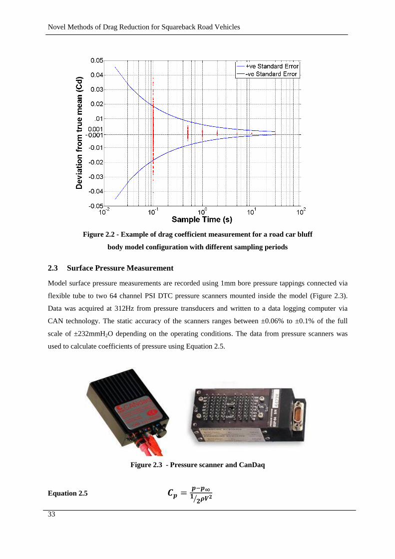
Novel Methods of Drag Reduction for Squareback Road Vehicles
33
Figure 2.2 - Example of drag coefficient measurement for a road car bluff
body model configuration with different sampling periods
2.3 Surface Pressure Measurement
Model surface pressure measurements are recorded using 1mm bore pressure tappings connected via
flexible tube to two 64 channel PSI DTC pressure scanners mounted inside the model (Figure 2.3).
Data was acquired at 312Hz from pressure transducers and written to a data logging computer via
CAN technology. The static accuracy of the scanners ranges between ±0.06% to ±0.1% of the full
scale of ±232mmH2O depending on the operating conditions. The data from pressure scanners was
used to calculate coefficients of pressure using Equation 2.5.
Figure 2.3 - Pressure scanner and CanDaq
Equation 2.5
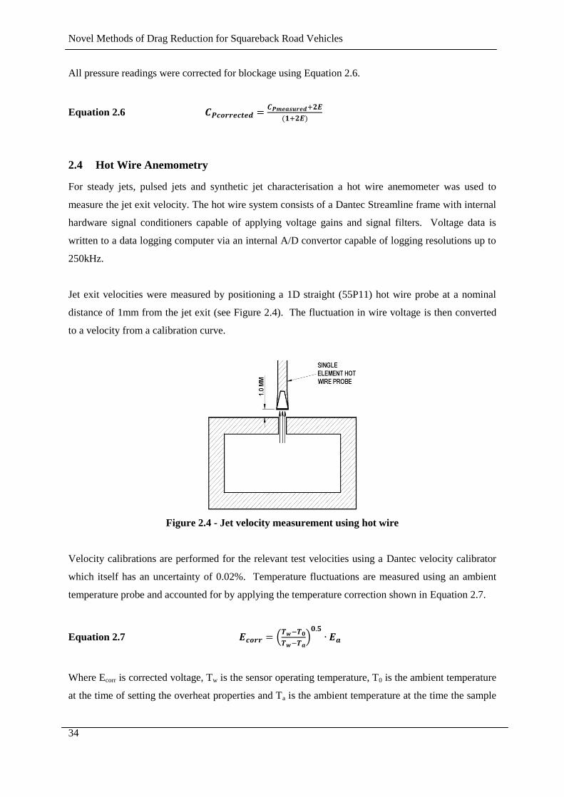
Novel Methods of Drag Reduction for Squareback Road Vehicles
34
All pressure readings were corrected for blockage using Equation 2.6.
Equation 2.6
2.4 Hot Wire Anemometry
For steady jets, pulsed jets and synthetic jet characterisation a hot wire anemometer was used to
measure the jet exit velocity. The hot wire system consists of a Dantec Streamline frame with internal
hardware signal conditioners capable of applying voltage gains and signal filters. Voltage data is
written to a data logging computer via an internal A/D convertor capable of logging resolutions up to
250kHz.
Jet exit velocities were measured by positioning a 1D straight (55P11) hot wire probe at a nominal
distance of 1mm from the jet exit (see Figure 2.4). The fluctuation in wire voltage is then converted
to a velocity from a calibration curve.
Figure 2.4 - Jet velocity measurement using hot wire
Velocity calibrations are performed for the relevant test velocities using a Dantec velocity calibrator
which itself has an uncertainty of 0.02%. Temperature fluctuations are measured using an ambient
temperature probe and accounted for by applying the temperature correction shown in Equation 2.7.
Equation 2.7
Where Ecorr is corrected voltage, Tw is the sensor operating temperature, T0 is the ambient temperature
at the time of setting the overheat properties and Ta is the ambient temperature at the time the sample
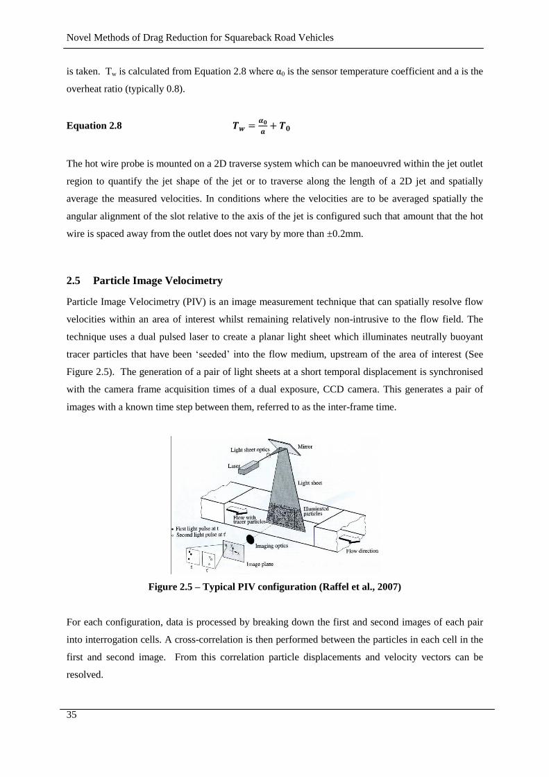
Novel Methods of Drag Reduction for Squareback Road Vehicles
35
is taken. Tw is calculated from Equation 2.8 where α0 is the sensor temperature coefficient and a is the
overheat ratio (typically 0.8).
Equation 2.8
The hot wire probe is mounted on a 2D traverse system which can be manoeuvred within the jet outlet
region to quantify the jet shape of the jet or to traverse along the length of a 2D jet and spatially
average the measured velocities. In conditions where the velocities are to be averaged spatially the
angular alignment of the slot relative to the axis of the jet is configured such that amount that the hot
wire is spaced away from the outlet does not vary by more than ±0.2mm.
2.5 Particle Image Velocimetry
Particle Image Velocimetry (PIV) is an image measurement technique that can spatially resolve flow
velocities within an area of interest whilst remaining relatively non-intrusive to the flow field. The
technique uses a dual pulsed laser to create a planar light sheet which illuminates neutrally buoyant
tracer particles that have been ‘seeded’ into the flow medium, upstream of the area of interest (See
Figure 2.5). The generation of a pair of light sheets at a short temporal displacement is synchronised
with the camera frame acquisition times of a dual exposure, CCD camera. This generates a pair of
images with a known time step between them, referred to as the inter-frame time.
Figure 2.5 – Typical PIV configuration (Raffel et al., 2007)
For each configuration, data is processed by breaking down the first and second images of each pair
into interrogation cells. A cross-correlation is then performed between the particles in each cell in the
first and second image. From this correlation particle displacements and velocity vectors can be
resolved.

Novel Methods of Drag Reduction for Squareback Road Vehicles
36
Instantaneous velocity flow fields for each image pair can be used to display statistical information
such as mean and RMS velocities, or further derivation can be used to generate information regarding
vorticity, swirl strength, turbulence intensity and typical length scales.
At each stage of the PIV process a number of parameters can be tuned in order to produce high
quality data. These various parameters are often not complementary so tradeoffs must be made. Some
rules and processing settings that have been consistently applied at the various stages of PIV
experimentation within this thesis are outlined below, whilst specific test setups will be described in
their relevant sections.
2.5.1 Seeding and Camera Field of View
Both oil and water seeding systems have been used during the PIV experimentation reported here,
where the average particle diameters are 2-5µm and 2-6µm respectively. Particle size, or more
specifically the diameter of the reflected laser light from the particle imaged by the CCD chip in
conjunction with the resolution and field of view of the camera(s) used are important factors to
consider if ‘peak locking’ is to be avoided.
Peak locking occurs when the reflection from a particle is less than or equal to one pixel in diameter.
If this is the case any shift in particle position from image one to image two can only be resolved to
±1 pixel. Ideally a particle reflection diameter should occupy 2-6 pixels (Hollis, 2004), in order that a
fitting function may be applied to the correlation data and particle displacement can be resolved at sub
pixel levels. Because particle diameters, and camera resolutions cannot easily be modified, peak
locking can be reduced during testing by reducing the field of view.
Peak locking can be detected by looking at a probability density function of the shifts detected in the
vector field. Figure 2.6 shows a PDF for vector field where velocities tend towards integer values of
pixel shifts, and it can be argued some of the particle images in this data are too small. Figure 2.7
shows a non-peak locked measurement where calculated shifts are distributed evenly between 0 and 1
fractions of pixel shift.
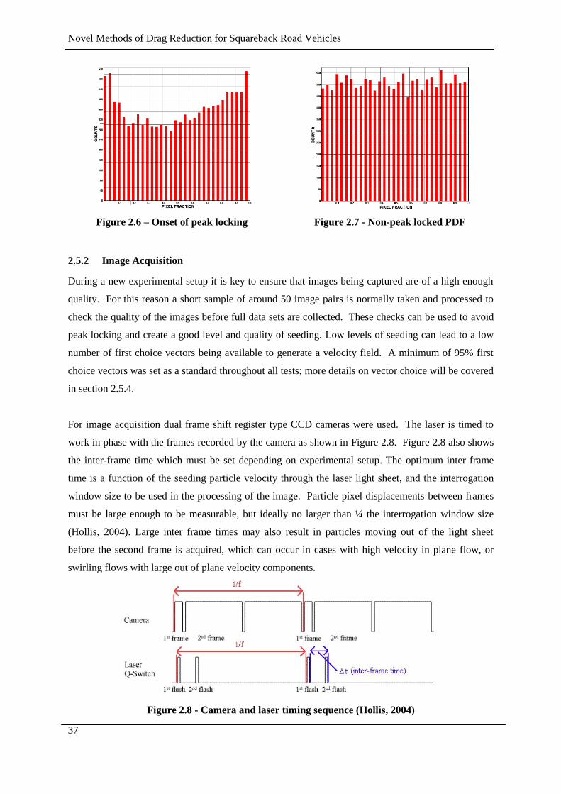
Novel Methods of Drag Reduction for Squareback Road Vehicles
37
Figure 2.6 – Onset of peak locking Figure 2.7 - Non-peak locked PDF
2.5.2 Image Acquisition
During a new experimental setup it is key to ensure that images being captured are of a high enough
quality. For this reason a short sample of around 50 image pairs is normally taken and processed to
check the quality of the images before full data sets are collected. These checks can be used to avoid
peak locking and create a good level and quality of seeding. Low levels of seeding can lead to a low
number of first choice vectors being available to generate a velocity field. A minimum of 95% first
choice vectors was set as a standard throughout all tests; more details on vector choice will be covered
in section 2.5.4.
For image acquisition dual frame shift register type CCD cameras were used. The laser is timed to
work in phase with the frames recorded by the camera as shown in Figure 2.8. Figure 2.8 also shows
the inter-frame time which must be set depending on experimental setup. The optimum inter frame
time is a function of the seeding particle velocity through the laser light sheet, and the interrogation
window size to be used in the processing of the image. Particle pixel displacements between frames
must be large enough to be measurable, but ideally no larger than ¼ the interrogation window size
(Hollis, 2004). Large inter frame times may also result in particles moving out of the light sheet
before the second frame is acquired, which can occur in cases with high velocity in plane flow, or
swirling flows with large out of plane velocity components.
Figure 2.8 - Camera and laser timing sequence (Hollis, 2004)

Novel Methods of Drag Reduction for Squareback Road Vehicles
38
The camera lens should be used to focus the CCD chip onto the plane of the light sheet such that
seeding particles are clearly identifiable. Ideally an F-stop setting would be used that creates the same
depth of field as the thickness of the light sheet. However due to the required trade off between
identification/illumination of particles and avoiding overexposure of the camera, depth of focus can
be larger than the light sheet thickness. This means that it is possible for particles outside of the plane
of interest to be included in calculations of velocity vector fields. Laser Intensity along with the lens
and f-stop setting must be tuned to arrive at the best configuration available.
Reflections of light from the model and tunnel walls can also have an influence on the correlations
performed to generate a vector field. To reduce the effect background reflections and bright spots
have on the data a background image is taken of each configuration without seeding. Before
processing the vector fields the background image is subtracted from every image pair.
2.5.3 Data Processing
In order to generate a velocity vector field from each instantaneous image pair the pixels within the
field of view are divided into ‘interrogation cells/windows’. A cross-correlation is performed
between the interrogation cells in the first image and the interrogation cells in the second image.
Where high levels of correlation occur a large spike can been seen in a correlation plot such as in
Figure 2.9. This spike can be used to generate a velocity vector for the interrogation window in
question. When a cross correlation has been performed for every interrogation window, a velocity
vector plot for the whole field of view can be generated.
Figure 2.9 - Example interrogation cell correlation plot
Multiple correlation passes with decreasing interrogation window sizes can be used to gradually shift
the position of the cells in the second frame to follow the expected path of the particles. This is
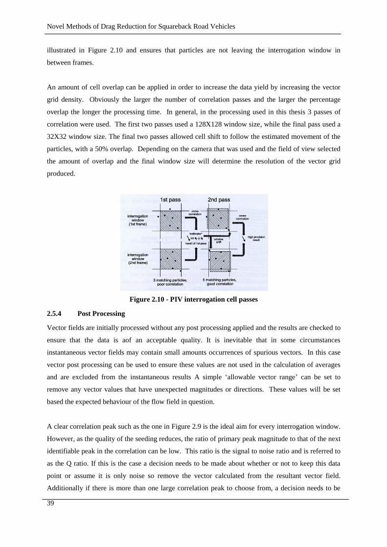
Novel Methods of Drag Reduction for Squareback Road Vehicles
39
illustrated in Figure 2.10 and ensures that particles are not leaving the interrogation window in
between frames.
An amount of cell overlap can be applied in order to increase the data yield by increasing the vector
grid density. Obviously the larger the number of correlation passes and the larger the percentage
overlap the longer the processing time. In general, in the processing used in this thesis 3 passes of
correlation were used. The first two passes used a 128X128 window size, while the final pass used a
32X32 window size. The final two passes allowed cell shift to follow the estimated movement of the
particles, with a 50% overlap. Depending on the camera that was used and the field of view selected
the amount of overlap and the final window size will determine the resolution of the vector grid
produced.
Figure 2.10 - PIV interrogation cell passes
2.5.4 Post Processing
Vector fields are initially processed without any post processing applied and the results are checked to
ensure that the data is aof an acceptable quality. It is inevitable that in some circumstances
instantaneous vector fields may contain small amounts occurrences of spurious vectors. In this case
vector post processing can be used to ensure these values are not used in the calculation of averages
and are excluded from the instantaneous results A simple ‘allowable vector range’ can be set to
remove any vector values that have unexpected magnitudes or directions. These values will be set
based the expected behaviour of the flow field in question.
A clear correlation peak such as the one in Figure 2.9 is the ideal aim for every interrogation window.
However, as the quality of the seeding reduces, the ratio of primary peak magnitude to that of the next
identifiable peak in the correlation can be low. This ratio is the signal to noise ratio and is referred to
as the Q ratio. If this is the case a decision needs to be made about whether or not to keep this data
point or assume it is only noise so remove the vector calculated from the resultant vector field.
Additionally if there is more than one large correlation peak to choose from, a decision needs to be
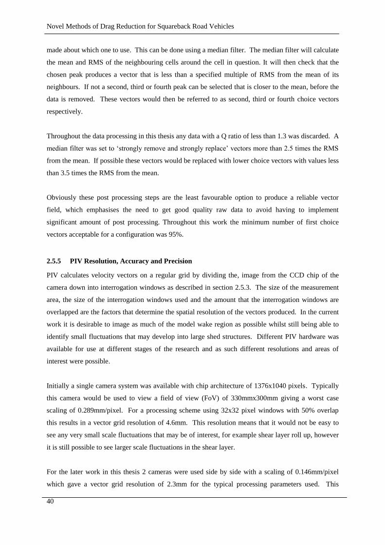
Novel Methods of Drag Reduction for Squareback Road Vehicles
40
made about which one to use. This can be done using a median filter. The median filter will calculate
the mean and RMS of the neighbouring cells around the cell in question. It will then check that the
chosen peak produces a vector that is less than a specified multiple of RMS from the mean of its
neighbours. If not a second, third or fourth peak can be selected that is closer to the mean, before the
data is removed. These vectors would then be referred to as second, third or fourth choice vectors
respectively.
Throughout the data processing in this thesis any data with a Q ratio of less than 1.3 was discarded. A
median filter was set to ‘strongly remove and strongly replace’ vectors more than 2.5 times the RMS
from the mean. If possible these vectors would be replaced with lower choice vectors with values less
than 3.5 times the RMS from the mean.
Obviously these post processing steps are the least favourable option to produce a reliable vector
field, which emphasises the need to get good quality raw data to avoid having to implement
significant amount of post processing. Throughout this work the minimum number of first choice
vectors acceptable for a configuration was 95%.
2.5.5 PIV Resolution, Accuracy and Precision
PIV calculates velocity vectors on a regular grid by dividing the, image from the CCD chip of the
camera down into interrogation windows as described in section 2.5.3. The size of the measurement
area, the size of the interrogation windows used and the amount that the interrogation windows are
overlapped are the factors that determine the spatial resolution of the vectors produced. In the current
work it is desirable to image as much of the model wake region as possible whilst still being able to
identify small fluctuations that may develop into large shed structures. Different PIV hardware was
available for use at different stages of the research and as such different resolutions and areas of
interest were possible.
Initially a single camera system was available with chip architecture of 1376x1040 pixels. Typically
this camera would be used to view a field of view (FoV) of 330mmx300mm giving a worst case
scaling of 0.289mm/pixel. For a processing scheme using 32x32 pixel windows with 50% overlap
this results in a vector grid resolution of 4.6mm. This resolution means that it would not be easy to
see any very small scale fluctuations that may be of interest, for example shear layer roll up, however
it is still possible to see larger scale fluctuations in the shear layer.
For the later work in this thesis 2 cameras were used side by side with a scaling of 0.146mm/pixel
which gave a vector grid resolution of 2.3mm for the typical processing parameters used. This

Novel Methods of Drag Reduction for Squareback Road Vehicles
41
configuration allows a significant measurement area whilst increasing on the vector grid resolution
from the initial setup. It can still be argued that the vector grid resolution is too large to pick up small
scale shear layer fluctuations or roll up but the data yield from this measurement is very large and a
number of small scale fluctuations can still be identified in instantaneous images. Figure 2.11 shows
an example instantaneous PIV vector field of a stream wise centre line plane in the wake of a square
back bluff body model. (see Figure 5.8 for specific measurement location, the back of the model is
shown on the right hand side of the plot as a black area). The plot is shown on a full page so that it is
not necessary to reduce the displayed vector resolution. This figure illustrates excellent level of detail
achievable in such a large field of view with a high grid resolution.
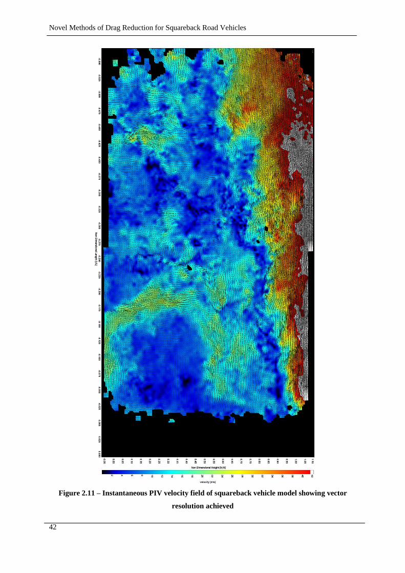
Novel Methods of Drag Reduction for Squareback Road Vehicles
42
Figure 2.11 – Instantaneous PIV velocity field of squareback vehicle model showing vector
resolution achieved
Novel Methods of Drag Reduction for Squareback Road Vehicles
43
A number of factors can influence the uncertainty of an instantaneous PIV measurement and the
overriding concern is that the raw images acquired are of a good quality. The steps taken to maximise
accuracy during the processing of the instantaneous images has been outlined in Section 2.5.3 and
2.5.4. However a finite measure of the total error at any one velocity vector can only be calculated if
the ‘true’ velocity is known.
The only way of starting from a known value is to generate synthetic images with a known ‘shift’ or
particle displacement. From these images the error associated with the ability of the correlation
algorithm to calculate the known shift can be determined. Figure 2.12 shows an example of synthetic
data with a low level of shift and a step change in shift in the centre, compared to the calculated
values of shift. For the calculated values, a level of fluctuation in the calculated values can be seen
and the spatially averaged RMS error can be regarded as the total error associated with the correlation
at a specified shift.
Figure 2.12 - a) Synthetic and b) calculated data
The RMS error will vary with the level of shift and the processing setting used, however typically the
algorithm used will resolve shifts of 0.1-10 pixels with an RMS error of 0.01 pixels. This error can be
converted to a displacement depending on the scaling used in the experiment, i.e. the Field of View
(FoV) and chip architecture.
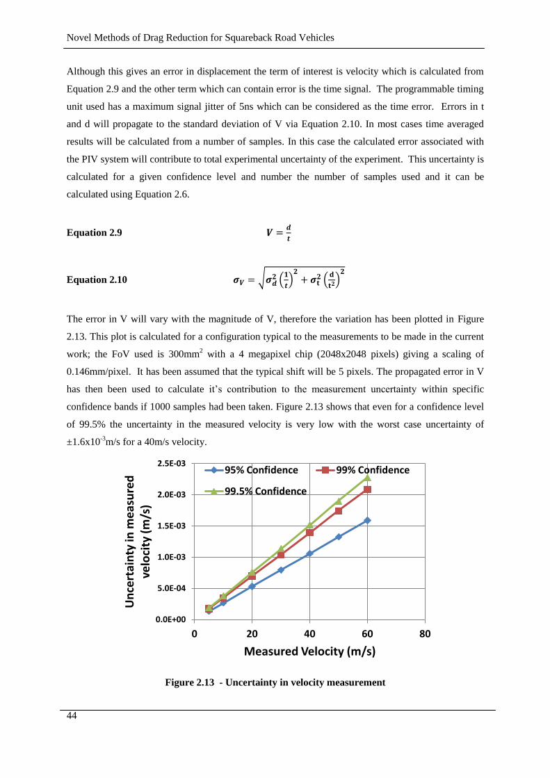
Novel Methods of Drag Reduction for Squareback Road Vehicles
44
Although this gives an error in displacement the term of interest is velocity which is calculated from
Equation 2.9 and the other term which can contain error is the time signal. The programmable timing
unit used has a maximum signal jitter of 5ns which can be considered as the time error. Errors in t
and d will propagate to the standard deviation of V via Equation 2.10. In most cases time averaged
results will be calculated from a number of samples. In this case the calculated error associated with
the PIV system will contribute to total experimental uncertainty of the experiment. This uncertainty is
calculated for a given confidence level and number the number of samples used and it can be
calculated using Equation 2.6.
Equation 2.9
Equation 2.10
The error in V will vary with the magnitude of V, therefore the variation has been plotted in Figure
2.13. This plot is calculated for a configuration typical to the measurements to be made in the current
work; the FoV used is 300mm2 with a 4 megapixel chip (2048x2048 pixels) giving a scaling of
0.146mm/pixel. It has been assumed that the typical shift will be 5 pixels. The propagated error in V
has then been used to calculate it’s contribution to the measurement uncertainty within specific
confidence bands if 1000 samples had been taken. Figure 2.13 shows that even for a confidence level
of 99.5% the uncertainty in the measured velocity is very low with the worst case uncertainty of
±1.6x10⁻³
m/s for a 40m/s velocity.
Figure 2.13 - Uncertainty in velocity measurement
0.0E+00
5.0E-04
1.0E-03
1.5E-03
2.0E-03
2.5E-03
0 20 40 60 80
Un
cert
ain
ty in
me
asu
red
ve
loci
ty (
m/s
)
Measured Velocity (m/s)
95% Confidence 99% Confidence
99.5% Confidence
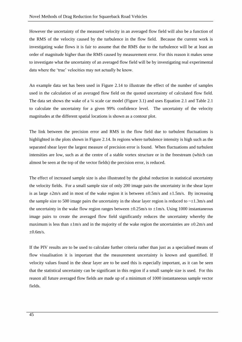
Novel Methods of Drag Reduction for Squareback Road Vehicles
45
However the uncertainty of the measured velocity in an averaged flow field will also be a function of
the RMS of the velocity caused by the turbulence in the flow field. Because the current work is
investigating wake flows it is fair to assume that the RMS due to the turbulence will be at least an
order of magnitude higher than the RMS caused by measurement error. For this reason it makes sense
to investigate what the uncertainty of an averaged flow field will be by investigating real experimental
data where the ‘true’ velocities may not actually be know.
An example data set has been used in Figure 2.14 to illustrate the effect of the number of samples
used in the calculation of an averaged flow field on the quoted uncertainty of calculated flow field.
The data set shows the wake of a ¼ scale car model (Figure 3.1) and uses Equation 2.1 and Table 2.1
to calculate the uncertainty for a given 99% confidence level. The uncertainty of the velocity
magnitudes at the different spatial locations is shown as a contour plot.
The link between the precision error and RMS in the flow field due to turbulent fluctuations is
highlighted in the plots shown in Figure 2.14. In regions where turbulence intensity is high such as the
separated shear layer the largest measure of precision error is found. When fluctuations and turbulent
intensities are low, such as at the centre of a stable vortex structure or in the freestream (which can
almost be seen at the top of the vector fields) the precision error, is reduced.
The effect of increased sample size is also illustrated by the global reduction in statistical uncertainty
the velocity fields. For a small sample size of only 200 image pairs the uncertainty in the shear layer
is as large ±2m/s and in most of the wake region it is between ±0.5m/s and ±1.5m/s. By increasing
the sample size to 500 image pairs the uncertainty in the shear layer region is reduced to ~±1.3m/s and
the uncertainty in the wake flow region ranges between ±0.25m/s to ±1m/s. Using 1000 instantaneous
image pairs to create the averaged flow field significantly reduces the uncertainty whereby the
maximum is less than ±1m/s and in the majority of the wake region the uncertainties are ±0.2m/s and
±0.6m/s.
If the PIV results are to be used to calculate further criteria rather than just as a specialised means of
flow visualisation it is important that the measurement uncertainty is known and quantified. If
velocity values found in the shear layer are to be used this is especially important, as it can be seen
that the statistical uncertainty can be significant in this region if a small sample size is used. For this
reason all future averaged flow fields are made up of a minimum of 1000 instantaneous sample vector
fields.
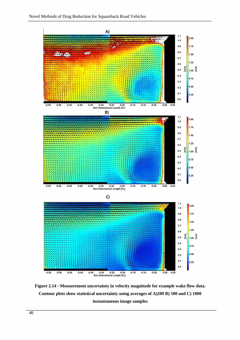
Novel Methods of Drag Reduction for Squareback Road Vehicles
46
Figure 2.14 - Measurement uncertainty in velocity magnitude for example wake flow data.
Contour plots show statistical uncertainty using averages of A)200 B) 500 and C) 1000
instantaneous image samples
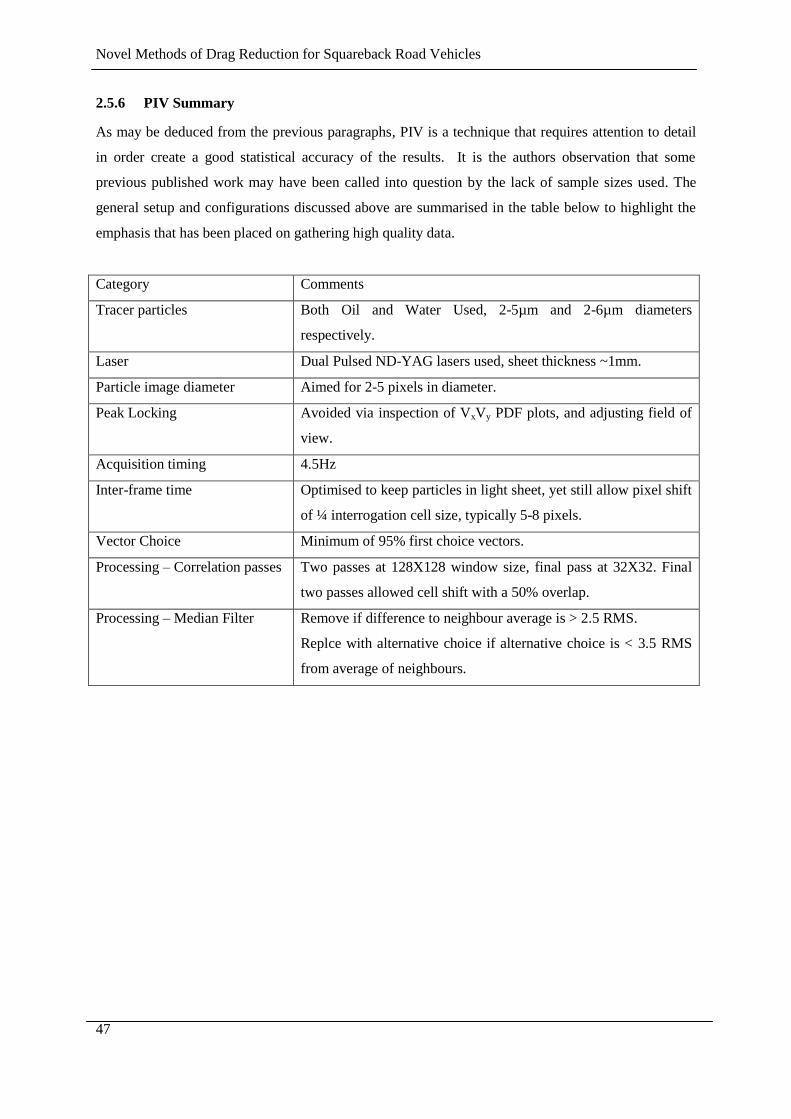
Novel Methods of Drag Reduction for Squareback Road Vehicles
47
2.5.6 PIV Summary
As may be deduced from the previous paragraphs, PIV is a technique that requires attention to detail
in order create a good statistical accuracy of the results. It is the authors observation that some
previous published work may have been called into question by the lack of sample sizes used. The
general setup and configurations discussed above are summarised in the table below to highlight the
emphasis that has been placed on gathering high quality data.
Category Comments
Tracer particles Both Oil and Water Used, 2-5µm and 2-6µm diameters
respectively.
Laser Dual Pulsed ND-YAG lasers used, sheet thickness ~1mm.
Particle image diameter Aimed for 2-5 pixels in diameter.
Peak Locking Avoided via inspection of VxVy PDF plots, and adjusting field of
view.
Acquisition timing 4.5Hz
Inter-frame time Optimised to keep particles in light sheet, yet still allow pixel shift
of ¼ interrogation cell size, typically 5-8 pixels.
Vector Choice Minimum of 95% first choice vectors.
Processing – Correlation passes Two passes at 128X128 window size, final pass at 32X32. Final
two passes allowed cell shift with a 50% overlap.
Processing – Median Filter Remove if difference to neighbour average is > 2.5 RMS.
Replce with alternative choice if alternative choice is < 3.5 RMS
from average of neighbours.

Novel Methods of Drag Reduction for Squareback Road Vehicles
48
Chapter 3
BASELINE VEHICLE CONFIGURATION
AND PASSIVE OPTIMISATION
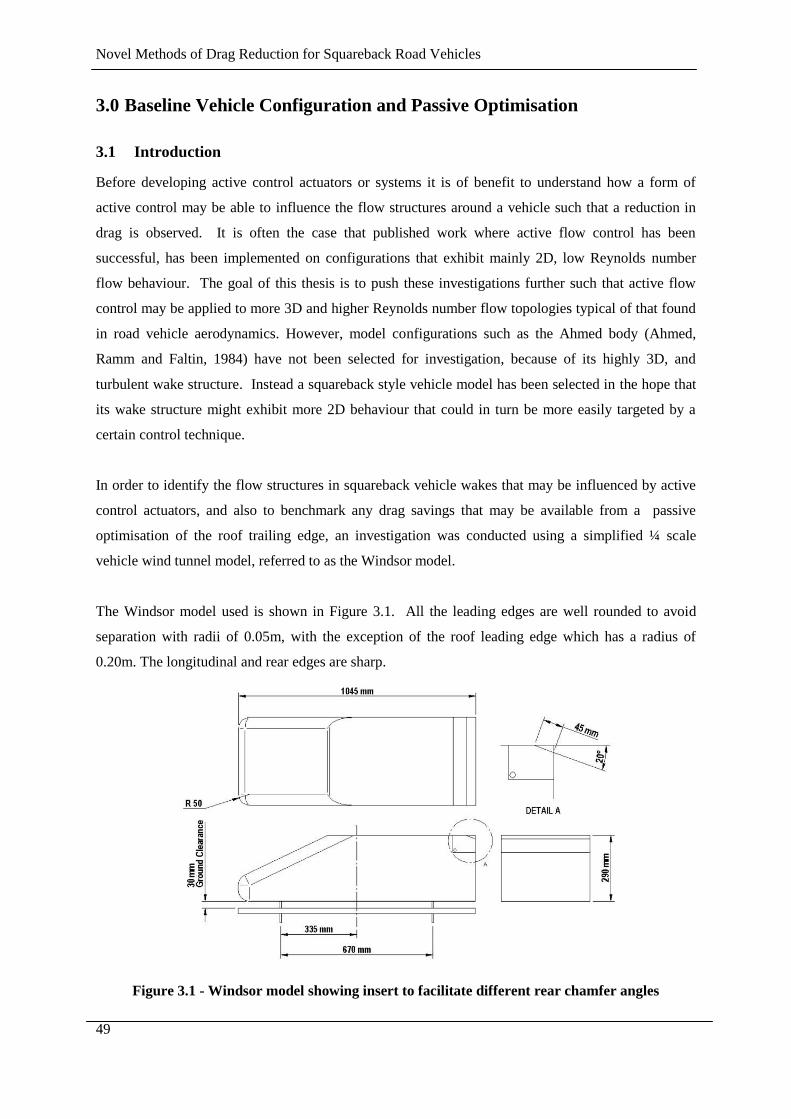
Novel Methods of Drag Reduction for Squareback Road Vehicles
49
3.0 Baseline Vehicle Configuration and Passive Optimisation
3.1 Introduction
Before developing active control actuators or systems it is of benefit to understand how a form of
active control may be able to influence the flow structures around a vehicle such that a reduction in
drag is observed. It is often the case that published work where active flow control has been
successful, has been implemented on configurations that exhibit mainly 2D, low Reynolds number
flow behaviour. The goal of this thesis is to push these investigations further such that active flow
control may be applied to more 3D and higher Reynolds number flow topologies typical of that found
in road vehicle aerodynamics. However, model configurations such as the Ahmed body (Ahmed,
Ramm and Faltin, 1984) have not been selected for investigation, because of its highly 3D, and
turbulent wake structure. Instead a squareback style vehicle model has been selected in the hope that
its wake structure might exhibit more 2D behaviour that could in turn be more easily targeted by a
certain control technique.
In order to identify the flow structures in squareback vehicle wakes that may be influenced by active
control actuators, and also to benchmark any drag savings that may be available from a passive
optimisation of the roof trailing edge, an investigation was conducted using a simplified ¼ scale
vehicle wind tunnel model, referred to as the Windsor model.
The Windsor model used is shown in Figure 3.1. All the leading edges are well rounded to avoid
separation with radii of 0.05m, with the exception of the roof leading edge which has a radius of
0.20m. The longitudinal and rear edges are sharp.
Figure 3.1 - Windsor model showing insert to facilitate different rear chamfer angles
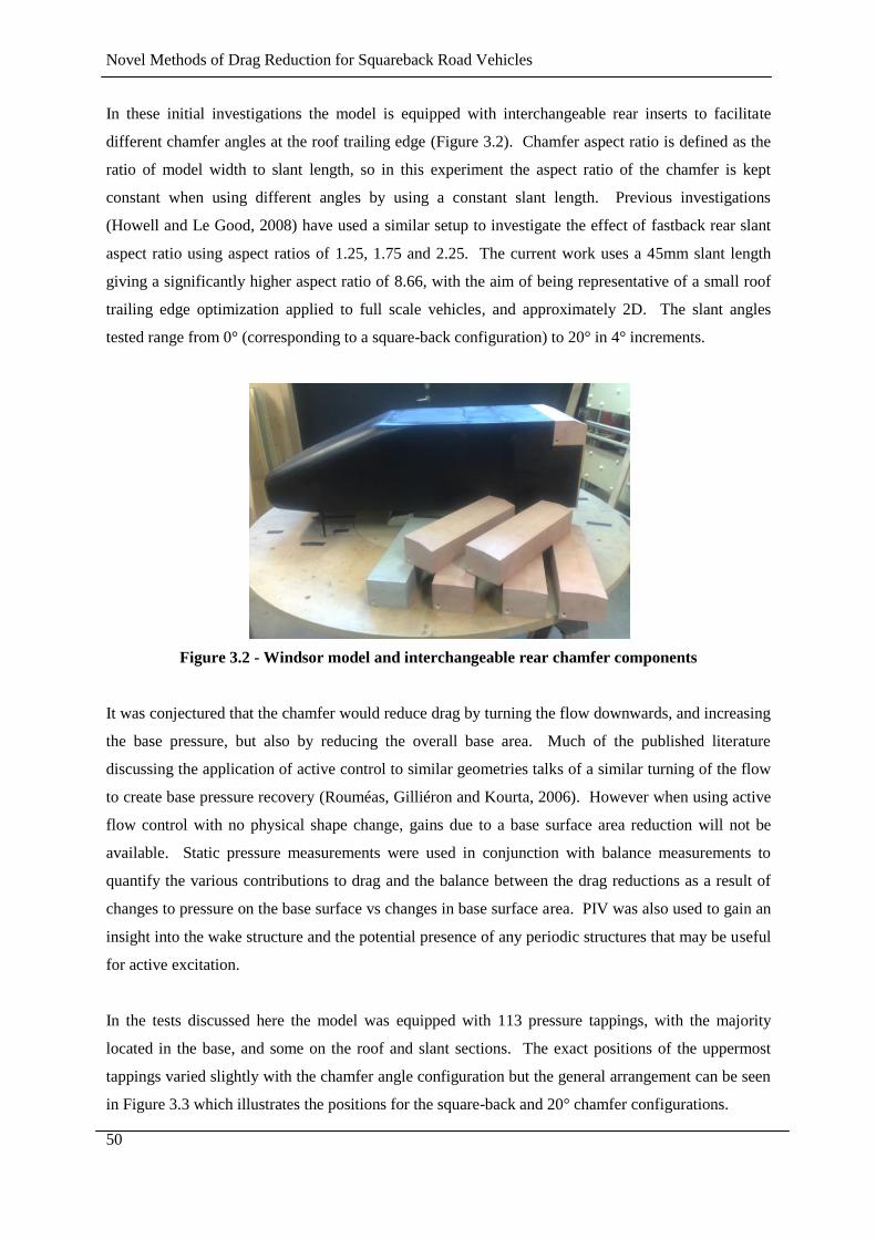
Novel Methods of Drag Reduction for Squareback Road Vehicles
50
In these initial investigations the model is equipped with interchangeable rear inserts to facilitate
different chamfer angles at the roof trailing edge (Figure 3.2). Chamfer aspect ratio is defined as the
ratio of model width to slant length, so in this experiment the aspect ratio of the chamfer is kept
constant when using different angles by using a constant slant length. Previous investigations
(Howell and Le Good, 2008) have used a similar setup to investigate the effect of fastback rear slant
aspect ratio using aspect ratios of 1.25, 1.75 and 2.25. The current work uses a 45mm slant length
giving a significantly higher aspect ratio of 8.66, with the aim of being representative of a small roof
trailing edge optimization applied to full scale vehicles, and approximately 2D. The slant angles
tested range from 0° (corresponding to a square-back configuration) to 20° in 4° increments.
Figure 3.2 - Windsor model and interchangeable rear chamfer components
It was conjectured that the chamfer would reduce drag by turning the flow downwards, and increasing
the base pressure, but also by reducing the overall base area. Much of the published literature
discussing the application of active control to similar geometries talks of a similar turning of the flow
to create base pressure recovery (Rouméas, Gilliéron and Kourta, 2006). However when using active
flow control with no physical shape change, gains due to a base surface area reduction will not be
available. Static pressure measurements were used in conjunction with balance measurements to
quantify the various contributions to drag and the balance between the drag reductions as a result of
changes to pressure on the base surface vs changes in base surface area. PIV was also used to gain an
insight into the wake structure and the potential presence of any periodic structures that may be useful
for active excitation.
In the tests discussed here the model was equipped with 113 pressure tappings, with the majority
located in the base, and some on the roof and slant sections. The exact positions of the uppermost
tappings varied slightly with the chamfer angle configuration but the general arrangement can be seen
in Figure 3.3 which illustrates the positions for the square-back and 20° chamfer configurations.
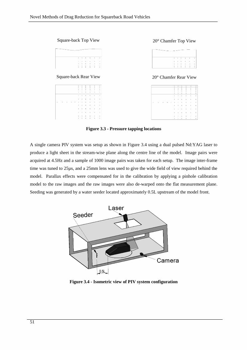
Novel Methods of Drag Reduction for Squareback Road Vehicles
51
Square-back Top View
Square-back Rear View
20° Chamfer Top View
20° Chamfer Rear View
Figure 3.3 - Pressure tapping locations
A single camera PIV system was setup as shown in Figure 3.4 using a dual pulsed Nd:YAG laser to
produce a light sheet in the stream-wise plane along the centre line of the model. Image pairs were
acquired at 4.5Hz and a sample of 1000 image pairs was taken for each setup. The image inter-frame
time was tuned to 25µs, and a 25mm lens was used to give the wide field of view required behind the
model. Parallax effects were compensated for in the calibration by applying a pinhole calibration
model to the raw images and the raw images were also de-warped onto the flat measurement plane.
Seeding was generated by a water seeder located approximately 0.5L upstream of the model front.
Figure 3.4 - Isometric view of PIV system configuration
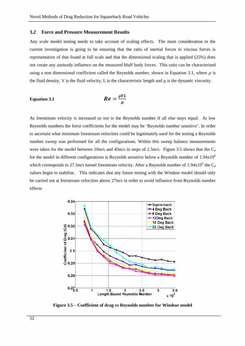
Novel Methods of Drag Reduction for Squareback Road Vehicles
52
3.2 Force and Pressure Measurement Results
Any scale model testing needs to take account of scaling effects. The main consideration in the
current investigation is going to be ensuring that the ratio of inertial forces to viscous forces is
representative of that found at full scale and that the dimensional scaling that is applied (25%) does
not create any unsteady influence on the measured bluff body forces. This ratio can be characterised
using a non dimensional coefficient called the Reynolds number, shown in Equation 3.1, where is
the fluid density, V is the fluid velocity, L is the characteristic length and µ is the dynamic viscosity.
Equation 3.1
As freestream velocity is increased so too is the Reynolds number if all else stays equal. At low
Reynolds numbers the force coefficients for the model may be ‘Reynolds number sensitive’. In order
to ascertain what minimum freestream velocities could be legitimately used for the testing a Reynolds
number sweep was performed for all the configurations. Within this sweep balance measurements
were taken for the model between 10m/s and 45m/s in steps of 2.5m/s. Figure 3.5 shows that the Cd
for the model in different configurations is Reynolds sensitive below a Reynolds number of 1.94x10⁶
which corresponds to 27.5m/s tunnel freestream velocity. After a Reynolds number of 1.94x10⁶ the Cd
values begin to stabilise. This indicates that any future testing with the Windsor model should only
be carried out at freestream velocities above 27m/s in order to avoid influence from Reynolds number
effects
Figure 3.5 – Coefficient of drag vs Reynolds number for Windsor model
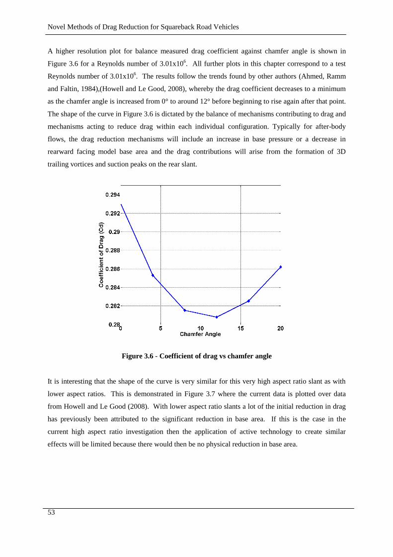
Novel Methods of Drag Reduction for Squareback Road Vehicles
53
A higher resolution plot for balance measured drag coefficient against chamfer angle is shown in
Figure 3.6 for a Reynolds number of 3.01x10⁶. All further plots in this chapter correspond to a test
Reynolds number of 3.01x10⁶. The results follow the trends found by other authors (Ahmed, Ramm
and Faltin, 1984),(Howell and Le Good, 2008), whereby the drag coefficient decreases to a minimum
as the chamfer angle is increased from 0° to around 12° before beginning to rise again after that point.
The shape of the curve in Figure 3.6 is dictated by the balance of mechanisms contributing to drag and
mechanisms acting to reduce drag within each individual configuration. Typically for after-body
flows, the drag reduction mechanisms will include an increase in base pressure or a decrease in
rearward facing model base area and the drag contributions will arise from the formation of 3D
trailing vortices and suction peaks on the rear slant.
Figure 3.6 - Coefficient of drag vs chamfer angle
It is interesting that the shape of the curve is very similar for this very high aspect ratio slant as with
lower aspect ratios. This is demonstrated in Figure 3.7 where the current data is plotted over data
from Howell and Le Good (2008). With lower aspect ratio slants a lot of the initial reduction in drag
has previously been attributed to the significant reduction in base area. If this is the case in the
current high aspect ratio investigation then the application of active technology to create similar
effects will be limited because there would then be no physical reduction in base area.
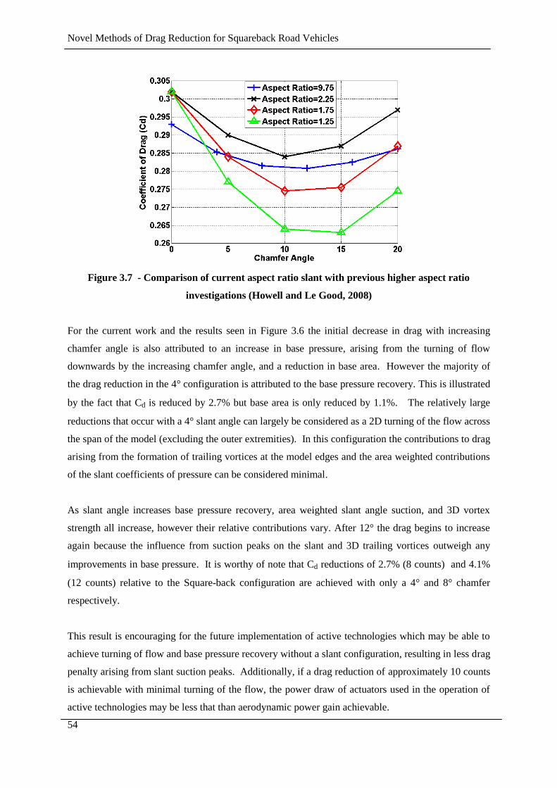
Novel Methods of Drag Reduction for Squareback Road Vehicles
54
Figure 3.7 - Comparison of current aspect ratio slant with previous higher aspect ratio
investigations (Howell and Le Good, 2008)
For the current work and the results seen in Figure 3.6 the initial decrease in drag with increasing
chamfer angle is also attributed to an increase in base pressure, arising from the turning of flow
downwards by the increasing chamfer angle, and a reduction in base area. However the majority of
the drag reduction in the 4° configuration is attributed to the base pressure recovery. This is illustrated
by the fact that Cd is reduced by 2.7% but base area is only reduced by 1.1%. The relatively large
reductions that occur with a 4° slant angle can largely be considered as a 2D turning of the flow across
the span of the model (excluding the outer extremities). In this configuration the contributions to drag
arising from the formation of trailing vortices at the model edges and the area weighted contributions
of the slant coefficients of pressure can be considered minimal.
As slant angle increases base pressure recovery, area weighted slant angle suction, and 3D vortex
strength all increase, however their relative contributions vary. After 12° the drag begins to increase
again because the influence from suction peaks on the slant and 3D trailing vortices outweigh any
improvements in base pressure. It is worthy of note that Cd reductions of 2.7% (8 counts) and 4.1%
(12 counts) relative to the Square-back configuration are achieved with only a 4° and 8° chamfer
respectively.
This result is encouraging for the future implementation of active technologies which may be able to
achieve turning of flow and base pressure recovery without a slant configuration, resulting in less drag
penalty arising from slant suction peaks. Additionally, if a drag reduction of approximately 10 counts
is achievable with minimal turning of the flow, the power draw of actuators used in the operation of
active technologies may be less that than aerodynamic power gain achievable.
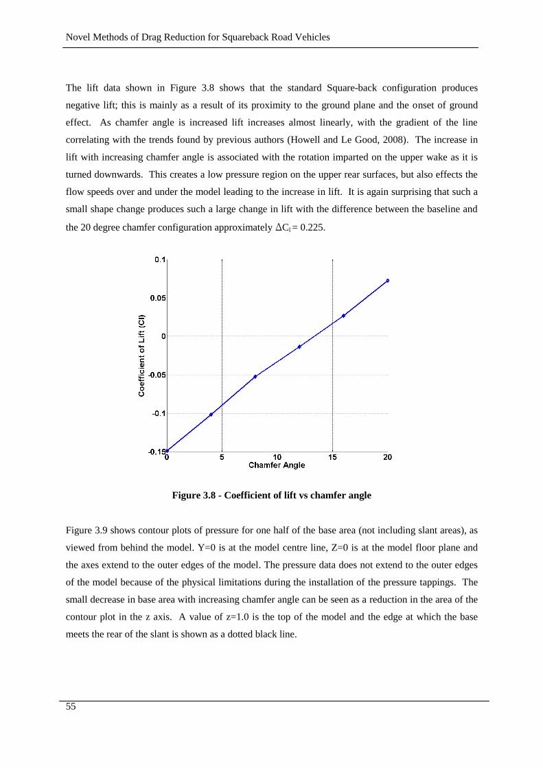
Novel Methods of Drag Reduction for Squareback Road Vehicles
55
The lift data shown in Figure 3.8 shows that the standard Square-back configuration produces
negative lift; this is mainly as a result of its proximity to the ground plane and the onset of ground
effect. As chamfer angle is increased lift increases almost linearly, with the gradient of the line
correlating with the trends found by previous authors (Howell and Le Good, 2008). The increase in
lift with increasing chamfer angle is associated with the rotation imparted on the upper wake as it is
turned downwards. This creates a low pressure region on the upper rear surfaces, but also effects the
flow speeds over and under the model leading to the increase in lift. It is again surprising that such a
small shape change produces such a large change in lift with the difference between the baseline and
the 20 degree chamfer configuration approximately ∆Cl = 0.225.
Figure 3.8 - Coefficient of lift vs chamfer angle
Figure 3.9 shows contour plots of pressure for one half of the base area (not including slant areas), as
viewed from behind the model. Y=0 is at the model centre line, Z=0 is at the model floor plane and
the axes extend to the outer edges of the model. The pressure data does not extend to the outer edges
of the model because of the physical limitations during the installation of the pressure tappings. The
small decrease in base area with increasing chamfer angle can be seen as a reduction in the area of the
contour plot in the z axis. A value of z=1.0 is the top of the model and the edge at which the base
meets the rear of the slant is shown as a dotted black line.
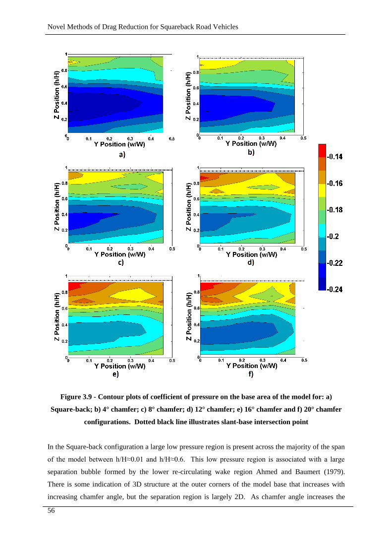
Novel Methods of Drag Reduction for Squareback Road Vehicles
56
Figure 3.9 - Contour plots of coefficient of pressure on the base area of the model for: a)
Square-back; b) 4° chamfer; c) 8° chamfer; d) 12° chamfer; e) 16° chamfer and f) 20° chamfer
configurations. Dotted black line illustrates slant-base intersection point
In the Square-back configuration a large low pressure region is present across the majority of the span
of the model between h/H≈0.01 and h/H≈0.6. This low pressure region is associated with a large
separation bubble formed by the lower re-circulating wake region Ahmed and Baumert (1979).
There is some indication of 3D structure at the outer corners of the model base that increases with
increasing chamfer angle, but the separation region is largely 2D. As chamfer angle increases the
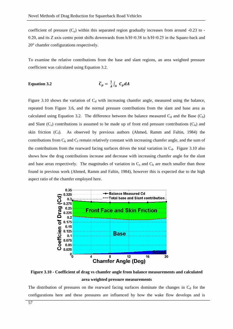
Novel Methods of Drag Reduction for Squareback Road Vehicles
57
coefficient of pressure (Cp) within this separated region gradually increases from around -0.23 to -
0.20, and its Z axis centre point shifts downwards from h/H≈0.38 to h/H≈0.25 in the Square-back and
20° chamfer configurations respectively.
To examine the relative contributions from the base and slant regions, an area weighted pressure
coefficient was calculated using Equation 3.2.
Equation 3.2
Figure 3.10 shows the variation of Cd with increasing chamfer angle, measured using the balance,
repeated from Figure 3.6, and the normal pressure contributions from the slant and base area as
calculated using Equation 3.2. The difference between the balance measured Cd and the Base (Cb)
and Slant (Cs) contributions is assumed to be made up of front end pressure contributions (Ck) and
skin friction (Cf). As observed by previous authors (Ahmed, Ramm and Faltin, 1984) the
contributions from Ck and Cf remain relatively constant with increasing chamfer angle, and the sum of
the contributions from the rearward facing surfaces drives the total variation in Cd. Figure 3.10 also
shows how the drag contributions increase and decrease with increasing chamfer angle for the slant
and base areas respectively. The magnitudes of variation in Cs and Cb are much smaller than those
found in previous work (Ahmed, Ramm and Faltin, 1984), however this is expected due to the high
aspect ratio of the chamfer employed here.
Figure 3.10 - Coefficient of drag vs chamfer angle from balance measurements and calculated
area weighted pressure measurements
The distribution of pressures on the rearward facing surfaces dominate the changes in Cd for the
configurations here and these pressures are influenced by how the wake flow develops and is
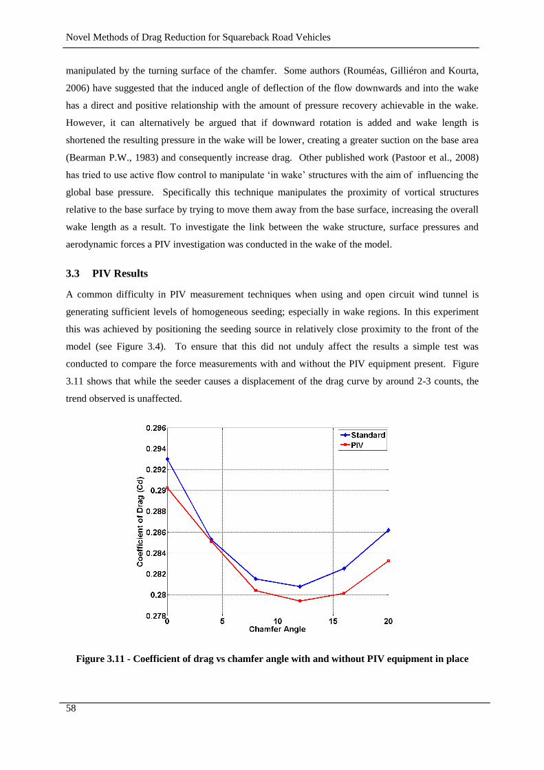
Novel Methods of Drag Reduction for Squareback Road Vehicles
58
manipulated by the turning surface of the chamfer. Some authors (Rouméas, Gilliéron and Kourta,
2006) have suggested that the induced angle of deflection of the flow downwards and into the wake
has a direct and positive relationship with the amount of pressure recovery achievable in the wake.
However, it can alternatively be argued that if downward rotation is added and wake length is
shortened the resulting pressure in the wake will be lower, creating a greater suction on the base area
(Bearman P.W., 1983) and consequently increase drag. Other published work (Pastoor et al., 2008)
has tried to use active flow control to manipulate ‘in wake’ structures with the aim of influencing the
global base pressure. Specifically this technique manipulates the proximity of vortical structures
relative to the base surface by trying to move them away from the base surface, increasing the overall
wake length as a result. To investigate the link between the wake structure, surface pressures and
aerodynamic forces a PIV investigation was conducted in the wake of the model.
3.3 PIV Results
A common difficulty in PIV measurement techniques when using and open circuit wind tunnel is
generating sufficient levels of homogeneous seeding; especially in wake regions. In this experiment
this was achieved by positioning the seeding source in relatively close proximity to the front of the
model (see Figure 3.4). To ensure that this did not unduly affect the results a simple test was
conducted to compare the force measurements with and without the PIV equipment present. Figure
3.11 shows that while the seeder causes a displacement of the drag curve by around 2-3 counts, the
trend observed is unaffected.
Figure 3.11 - Coefficient of drag vs chamfer angle with and without PIV equipment in place
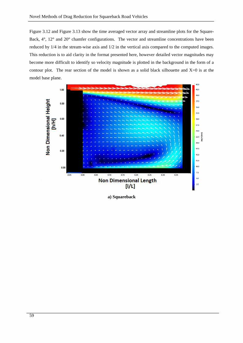
Novel Methods of Drag Reduction for Squareback Road Vehicles
59
Figure 3.12 and Figure 3.13 show the time averaged vector array and streamline plots for the Square-
Back, 4°, 12° and 20° chamfer configurations. The vector and streamline concentrations have been
reduced by 1/4 in the stream-wise axis and 1/2 in the vertical axis compared to the computed images.
This reduction is to aid clarity in the format presented here, however detailed vector magnitudes may
become more difficult to identify so velocity magnitude is plotted in the background in the form of a
contour plot. The rear section of the model is shown as a solid black silhouette and X=0 is at the
model base plane.
a) Squareback
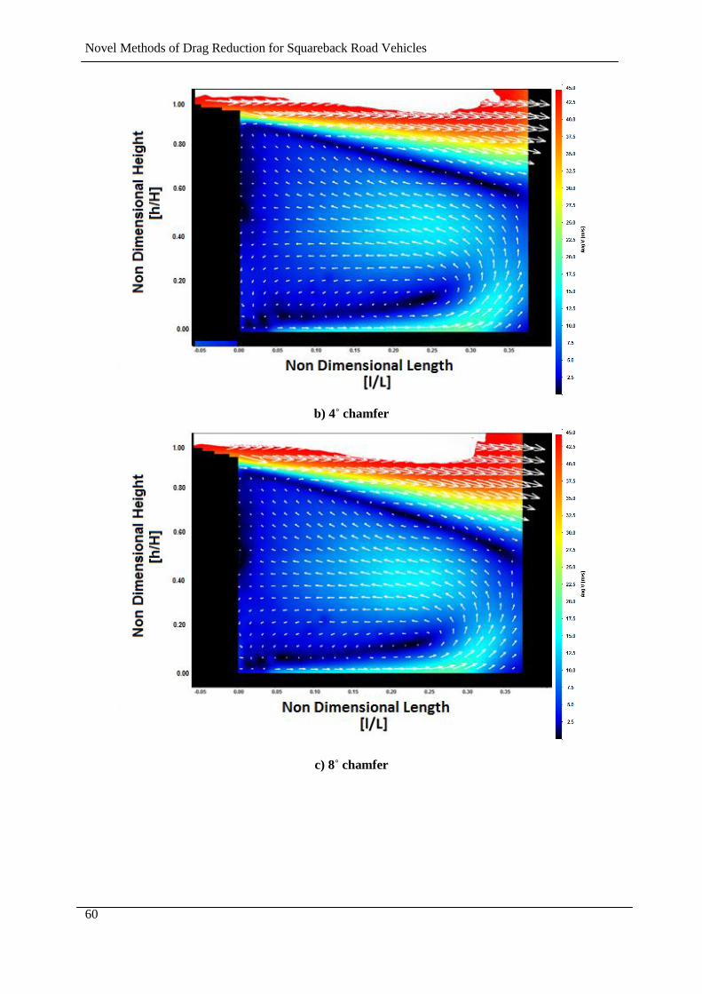
Novel Methods of Drag Reduction for Squareback Road Vehicles
60
b) 4˚ chamfer
c) 8˚ chamfer
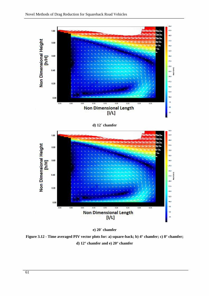
Novel Methods of Drag Reduction for Squareback Road Vehicles
61
d) 12˚ chamfer
e) 20˚ chamfer
Figure 3.12 - Time averaged PIV vector plots for: a) square-back; b) 4° chamfer; c) 8° chamfer;
d) 12° chamfer and e) 20° chamfer
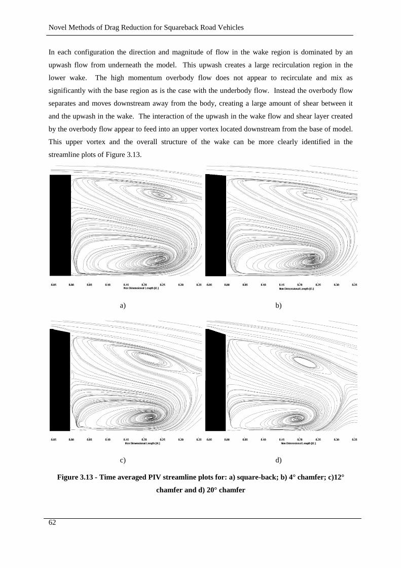
Novel Methods of Drag Reduction for Squareback Road Vehicles
62
In each configuration the direction and magnitude of flow in the wake region is dominated by an
upwash flow from underneath the model. This upwash creates a large recirculation region in the
lower wake. The high momentum overbody flow does not appear to recirculate and mix as
significantly with the base region as is the case with the underbody flow. Instead the overbody flow
separates and moves downstream away from the body, creating a large amount of shear between it
and the upwash in the wake. The interaction of the upwash in the wake flow and shear layer created
by the overbody flow appear to feed into an upper vortex located downstream from the base of model.
This upper vortex and the overall structure of the wake can be more clearly identified in the
streamline plots of Figure 3.13.
a)
b)
c)
d)
Figure 3.13 - Time averaged PIV streamline plots for: a) square-back; b) 4° chamfer; c)12°
chamfer and d) 20° chamfer
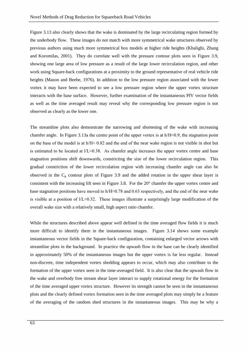
Novel Methods of Drag Reduction for Squareback Road Vehicles
63
Figure 3.13 also clearly shows that the wake is dominated by the large recirculating region formed by
the underbody flow. These images do not match with more symmetrical wake structures observed by
previous authors using much more symmetrical box models at higher ride heights (Khalighi, Zhang
and Koromilas, 2001). They do correlate well with the pressure contour plots seen in Figure 3.9,
showing one large area of low pressure as a result of the large lower recirculation region, and other
work using Square-back configurations at a proximity to the ground representative of real vehicle ride
heights (Mason and Beebe, 1976). In addition to the low pressure region associated with the lower
vortex it may have been expected to see a low pressure region where the upper vortex structure
interacts with the base surface. However, further examination of the instantaneous PIV vector fields
as well as the time averaged result may reveal why the corresponding low pressure region is not
observed as clearly as the lower one.
The streamline plots also demonstrate the narrowing and shortening of the wake with increasing
chamfer angle. In Figure 3.13a the centre point of the upper vortex is at h/H≈0.9, the stagnation point
on the base of the model is at h/H≈ 0.82 and the end of the near wake region is not visible in shot but
is estimated to be located at l/L≈0.38. As chamfer angle increases the upper vortex centre and base
stagnation positions shift downwards, constricting the size of the lower recirculation region. This
gradual constriction of the lower recirculation region with increasing chamfer angle can also be
observed in the Cp contour plots of Figure 3.9 and the added rotation in the upper shear layer is
consistent with the increasing lift seen in Figure 3.8. For the 20° chamfer the upper vortex centre and
base stagnation positions have moved to h/H≈0.78 and 0.63 respectively, and the end of the near wake
is visible at a position of l/L≈0.32. These images illustrate a surprisingly large modification of the
overall wake size with a relatively small, high aspect ratio chamfer.
While the structures described above appear well defined in the time averaged flow fields it is much
more difficult to identify them in the instantaneous images. Figure 3.14 shows some example
instantaneous vector fields in the Square-back configuration, containing enlarged vector arrows with
streamline plots in the background. In practice the upwash flow in the base can be clearly identified
in approximately 50% of the instantaneous images but the upper vortex is far less regular. Instead
non-discrete, time independent vortex shedding appears to occur, which may also contribute to the
formation of the upper vortex seen in the time-averaged field. It is also clear that the upwash flow in
the wake and overbody free stream shear layer interact to supply rotational energy for the formation
of the time averaged upper vortex structure. However its strength cannot be seen in the instantaneous
plots and the clearly defined vortex formation seen in the time averaged plots may simply be a feature
of the averaging of the random shed structures in the instantaneous images. This may be why a
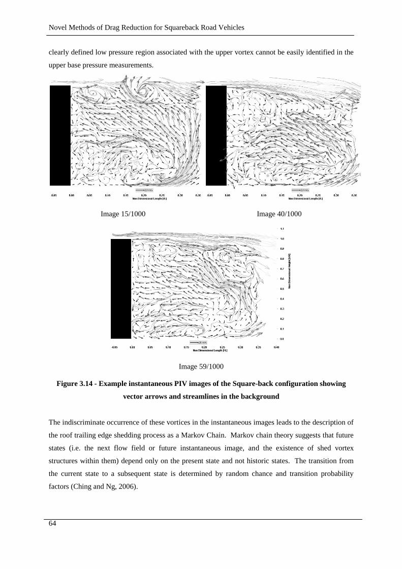
Novel Methods of Drag Reduction for Squareback Road Vehicles
64
clearly defined low pressure region associated with the upper vortex cannot be easily identified in the
upper base pressure measurements.
Image 15/1000
Image 40/1000
Image 59/1000
Figure 3.14 - Example instantaneous PIV images of the Square-back configuration showing
vector arrows and streamlines in the background
The indiscriminate occurrence of these vortices in the instantaneous images leads to the description of
the roof trailing edge shedding process as a Markov Chain. Markov chain theory suggests that future
states (i.e. the next flow field or future instantaneous image, and the existence of shed vortex
structures within them) depend only on the present state and not historic states. The transition from
the current state to a subsequent state is determined by random chance and transition probability
factors (Ching and Ng, 2006).
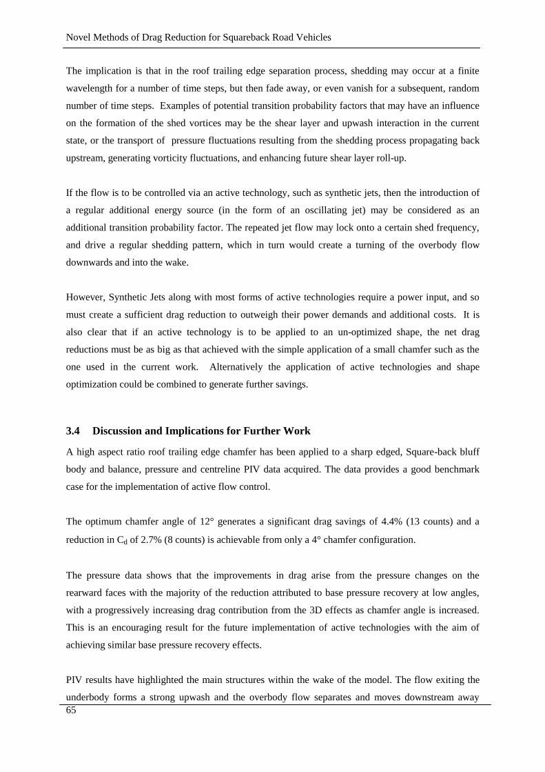
Novel Methods of Drag Reduction for Squareback Road Vehicles
65
The implication is that in the roof trailing edge separation process, shedding may occur at a finite
wavelength for a number of time steps, but then fade away, or even vanish for a subsequent, random
number of time steps. Examples of potential transition probability factors that may have an influence
on the formation of the shed vortices may be the shear layer and upwash interaction in the current
state, or the transport of pressure fluctuations resulting from the shedding process propagating back
upstream, generating vorticity fluctuations, and enhancing future shear layer roll-up.
If the flow is to be controlled via an active technology, such as synthetic jets, then the introduction of
a regular additional energy source (in the form of an oscillating jet) may be considered as an
additional transition probability factor. The repeated jet flow may lock onto a certain shed frequency,
and drive a regular shedding pattern, which in turn would create a turning of the overbody flow
downwards and into the wake.
However, Synthetic Jets along with most forms of active technologies require a power input, and so
must create a sufficient drag reduction to outweigh their power demands and additional costs. It is
also clear that if an active technology is to be applied to an un-optimized shape, the net drag
reductions must be as big as that achieved with the simple application of a small chamfer such as the
one used in the current work. Alternatively the application of active technologies and shape
optimization could be combined to generate further savings.
3.4 Discussion and Implications for Further Work
A high aspect ratio roof trailing edge chamfer has been applied to a sharp edged, Square-back bluff
body and balance, pressure and centreline PIV data acquired. The data provides a good benchmark
case for the implementation of active flow control.
The optimum chamfer angle of 12° generates a significant drag savings of 4.4% (13 counts) and a
reduction in Cd of 2.7% (8 counts) is achievable from only a 4° chamfer configuration.
The pressure data shows that the improvements in drag arise from the pressure changes on the
rearward faces with the majority of the reduction attributed to base pressure recovery at low angles,
with a progressively increasing drag contribution from the 3D effects as chamfer angle is increased.
This is an encouraging result for the future implementation of active technologies with the aim of
achieving similar base pressure recovery effects.
PIV results have highlighted the main structures within the wake of the model. The flow exiting the
underbody forms a strong upwash and the overbody flow separates and moves downstream away
Novel Methods of Drag Reduction for Squareback Road Vehicles
66
from the body, creating a large amount of shear that interacts with the wake to feed into an upper
vortex set downstream from the base of the model. However this vortex is not clearly defined in
instantaneous data and can be regarded as a very transient feature or perhaps even a statistical feature
of the averaging process.
In general the instantaneous images of the flow field do not indicate a well defined time averaged
wake structure. Instead flow structures that contribute to the formation of the time averaged pattern
are present, but are not regular. The random roof trailing edge shedding is likened to a Markov chain.
It is conjectured that probability of vortex structures occurring may be increased by the
implementation of an active technology such as synthetic jet actuators.
The work so far has demonstrated how difficult it is to identify a regular set of shed structures from
the rear edges of the model. However ‘shedding’ has been observed and it is conjectured that this
process may be promoted or suppressed by active flow control to influence base pressures. In order to
generate an active flow control experiment the actuators themselves must first be investigated. The
next chapter will describe the investigatory work that was conducted to try and design an effective
active flow control device, such as a Synthetic Jet or a pulsed jet.
Novel Methods of Drag Reduction for Squareback Road Vehicles
67
Chapter 4
ACTIVE CONTROL ACTUATOR
DESIGN AND TESTING

Novel Methods of Drag Reduction for Squareback Road Vehicles
68
4.0 Active Control Actuator Design and Testing
4.1 Introduction
A number of factors will determine how well and how efficiently an active flow control device (in this
case some form of air jet) will be able to influence the external cross flow in question. Various
investigations have described the requirements for formation of a jet, penetration length of jets, outlet
velocity profiles and magnitudes of jets. In addition to how well a jet performs it must have the
potential to be applied to a road vehicle, where additional criteria become introduced. Some of which
are overall size and weight, energy conversion efficiency and cost. Due to the potential for compact
sizes and low energy demands the Synthetic jet has been identified as a desirable technology to
investigate.
Unfortunately a number of variables influence how well a synthetic jet will perform, and there is no
such thing as a ‘common off the shelf’ solution. For this reason a bespoke synthetic jet arrangement
must be designed and its performance in a simple test case assessed. This investigation will not only
give an insight into the potential for synthetic jets to work in simple test cases but also highlight any
potential problems if they are to be applied to more complex model testing or even scaled to full scale
vehicles.
The oscillations that drive fluid in and out of a synthetic jet orifice are usually driven in one of three
ways.
• Piezoelectrically driven diaphragms
• Electromagnetically driven pistons
• Acoustically driven cavities
Additionally the orifice that forms the outlet/inlet for the jet can be designed as either a slot or a
circular hole. In each of the three drive methods, through either a slot or a hole, the formation of a jet
is characterised by the separation and roll up of vortices which advect away from the orifice. If the so
called ‘Acoustic Streaming Criterion’ (McKormick, 2000) (ASC) shown in Figure 4.1 is met the
vortices will separate away from the orifice without significant interaction with the in-stroke phase of
the process, and eventually decay to smaller length scales.

Novel Methods of Drag Reduction for Squareback Road Vehicles
69
Figure 4.1 - Acoustic streaming criterion (McKormick, 2000)
The ASC illustrates that for low levels of excitation, fluid particles will move in and out of the orifice
a small amount without mixing with particles outside of the orifice (regions 1 and 2). In region 3
significant turbulence is generated around the orifice and some acoustic energy is converted into mean
fluid motion. In region 4, the “Acoustic Jet Region”, particle displacement extends well outside the
orifice, allowing separation from the orifice exit and the roll up of vortices which advect away to form
a jet (Figure 4.2). The vortex formation can create a pair of axissymmetric vortices (2D jet) in the
case of a slot, or a circular axissymetric ring vortex (3D jet) in the case of a circular hole.
Figure 4.2 - Synthetic jet with characteristic vortices (Glezer and Amitay, 2002)
Many authors (Holman and Utturkar, 2005), (Sharma, 2006), (Guo and Zhong, 2006), (Lockerby and
Carpenter, 2004), (Kim and Gary, 2006) have conducted experiments and tried to create models of jet
performance and vortex formation based on physical parameters of the orifice and cavity. The focus
of most of the work is to ensure vortex formation occurs and the maximum amount of momentum is
expelled in the outstroke for a given amount of input energy. For a jet in a quiescent medium a
Reynolds number based on the momentum from the jet can be expressed in the form shown in
Equation 4.1.
Equation 4.1
Where b is the jet orifice diameter or orifice width µ is the dynamic viscosity of the fluid and I0 is
defined by Equation 4.2.
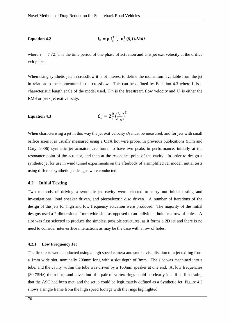
Novel Methods of Drag Reduction for Squareback Road Vehicles
70
Equation 4.2
where , T is the time period of one phase of actuation and uj is jet exit velocity at the orifice
exit plane.
When using synthetic jets in crossflow it is of interest to define the momentum available from the jet
in relation to the momentum in the crossflow. This can be defined by Equation 4.3 where L is a
characteristic length scale of the model used, U∞ is the freestream flow velocity and Uj is either the
RMS or peak jet exit velocity.
Equation 4.3
When characterising a jet in this way the jet exit velocity must be measured, and for jets with small
orifice sizes it is usually measured using a CTA hot wire probe. In previous publications (Kim and
Gary, 2006) synthetic jet actuators are found to have two peaks in performance, initially at the
resonance point of the actuator, and then at the resonance point of the cavity. In order to design a
synthetic jet for use in wind tunnel experiments on the afterbody of a simplified car model, initial tests
using different synthetic jet designs were conducted.
4.2 Initial Testing
Two methods of driving a synthetic jet cavity were selected to carry out initial testing and
investigations; loud speaker driven, and piezoelectric disc driven. A number of iterations of the
design of the jets for high and low frequency actuation were produced. The majority of the initial
designs used a 2 dimensional 1mm wide slot, as opposed to an individual hole or a row of holes. A
slot was first selected to produce the simplest possible structures, as it forms a 2D jet and there is no
need to consider inter-orifice interactions as may be the case with a row of holes.
4.2.1 Low Frequency Jet
The first tests were conducted using a high speed camera and smoke visualisation of a jet exiting from
a 1mm wide slot, nominally 200mm long with a slot depth of 3mm. The slot was machined into a
tube, and the cavity within the tube was driven by a 160mm speaker at one end. At low frequencies
(30-75Hz) the roll up and advection of a pair of vortex rings could be clearly identified illustrating
that the ASC had been met, and the setup could be legitimately defined as a Synthetic Jet. Figure 4.3
shows a single frame from the high speed footage with the rings highlighted.

Novel Methods of Drag Reduction for Squareback Road Vehicles
71
Figure 4.3 - Single frame from high speed camera images of synthetic jet at 50Hz
Additional images were taken with the camera at 90 degrees to the slot axis to investigate how
homogeneous the jet exit profile along the length of the slot was. Interestingly at a drive frequency of
90Hz a standing wave was set up within the tube. This was observed whereby vortex rings could
clearly be seen when the slot was viewed along its axis, but off axis a sinusoidal wave of smoke was
observed.
Whether or not this wave would be detrimental to the flow control ability of a synthetic jet is
unknown, however it would introduce an additional variable to any testing. Therefore it is noted that
standing waves should be avoided in any actual tests on a wind tunnel model. The configuration
described above used a single speaker at one end of the cylinder, and this would have increased the
likely hood that this behaviour was created. For future designs asymmetry in the actuator positioning
was avoided.
Exit velocity data was recorded using a CTA hot wire probe, placed at the slot exit plane as described
in section 2.4 however the hot wire was calibrated in the Loughborough University wind tunnel for
velocities between 5-40m/s as the Dantec calibrator was not available at this point. Figure 4.4, shows
an extract from the measured velocity data for a jet driven at 50 Hz. The data shows that peak
velocities were clipped at 40m/s, indicating that they were out of the calibration range. Future
calibrations were made using a Dantec calibrator from 0-60 m/s to avoid this effect.
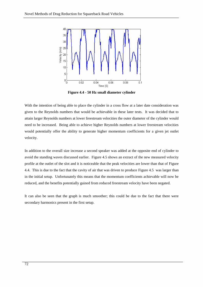
Novel Methods of Drag Reduction for Squareback Road Vehicles
72
Figure 4.4 - 50 Hz small diameter cylinder
With the intention of being able to place the cylinder in a cross flow at a later date consideration was
given to the Reynolds numbers that would be achievable in these later tests. It was decided that to
attain larger Reynolds numbers at lower freestream velocities the outer diameter of the cylinder would
need to be increased. Being able to achieve higher Reynolds numbers at lower freestream velocities
would potentially offer the ability to generate higher momentum coefficients for a given jet outlet
velocity.
In addition to the overall size increase a second speaker was added at the opposite end of cylinder to
avoid the standing waves discussed earlier. Figure 4.5 shows an extract of the new measured velocity
profile at the outlet of the slot and it is noticeable that the peak velocities are lower than that of Figure
4.4. This is due to the fact that the cavity of air that was driven to produce Figure 4.5 was larger than
in the initial setup. Unfortunately this means that the momentum coefficients achievable will now be
reduced, and the benefits potentially gained from reduced freestream velocity have been negated.
It can also be seen that the graph is much smoother; this could be due to the fact that there were
secondary harmonics present in the first setup.
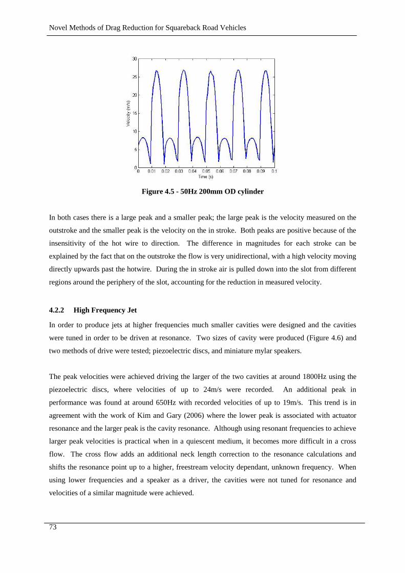
Novel Methods of Drag Reduction for Squareback Road Vehicles
73
Figure 4.5 - 50Hz 200mm OD cylinder
In both cases there is a large peak and a smaller peak; the large peak is the velocity measured on the
outstroke and the smaller peak is the velocity on the in stroke. Both peaks are positive because of the
insensitivity of the hot wire to direction. The difference in magnitudes for each stroke can be
explained by the fact that on the outstroke the flow is very unidirectional, with a high velocity moving
directly upwards past the hotwire. During the in stroke air is pulled down into the slot from different
regions around the periphery of the slot, accounting for the reduction in measured velocity.
4.2.2 High Frequency Jet
In order to produce jets at higher frequencies much smaller cavities were designed and the cavities
were tuned in order to be driven at resonance. Two sizes of cavity were produced (Figure 4.6) and
two methods of drive were tested; piezoelectric discs, and miniature mylar speakers.
The peak velocities were achieved driving the larger of the two cavities at around 1800Hz using the
piezoelectric discs, where velocities of up to 24m/s were recorded. An additional peak in
performance was found at around 650Hz with recorded velocities of up to 19m/s. This trend is in
agreement with the work of Kim and Gary (2006) where the lower peak is associated with actuator
resonance and the larger peak is the cavity resonance. Although using resonant frequencies to achieve
larger peak velocities is practical when in a quiescent medium, it becomes more difficult in a cross
flow. The cross flow adds an additional neck length correction to the resonance calculations and
shifts the resonance point up to a higher, freestream velocity dependant, unknown frequency. When
using lower frequencies and a speaker as a driver, the cavities were not tuned for resonance and
velocities of a similar magnitude were achieved.
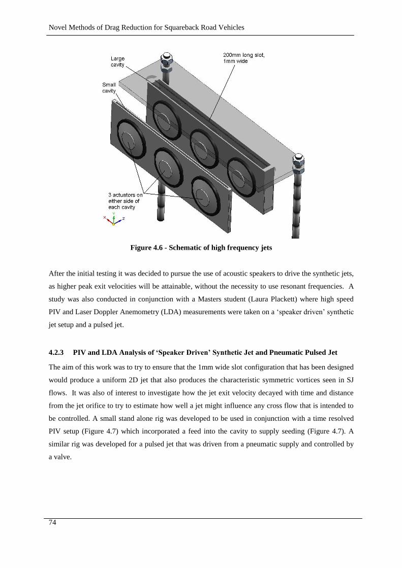
Novel Methods of Drag Reduction for Squareback Road Vehicles
74
Figure 4.6 - Schematic of high frequency jets
After the initial testing it was decided to pursue the use of acoustic speakers to drive the synthetic jets,
as higher peak exit velocities will be attainable, without the necessity to use resonant frequencies. A
study was also conducted in conjunction with a Masters student (Laura Plackett) where high speed
PIV and Laser Doppler Anemometry (LDA) measurements were taken on a ‘speaker driven’ synthetic
jet setup and a pulsed jet.
4.2.3 PIV and LDA Analysis of ‘Speaker Driven’ Synthetic Jet and Pneumatic Pulsed Jet
The aim of this work was to try to ensure that the 1mm wide slot configuration that has been designed
would produce a uniform 2D jet that also produces the characteristic symmetric vortices seen in SJ
flows. It was also of interest to investigate how the jet exit velocity decayed with time and distance
from the jet orifice to try to estimate how well a jet might influence any cross flow that is intended to
be controlled. A small stand alone rig was developed to be used in conjunction with a time resolved
PIV setup (Figure 4.7) which incorporated a feed into the cavity to supply seeding (Figure 4.7). A
similar rig was developed for a pulsed jet that was driven from a pneumatic supply and controlled by
a valve.
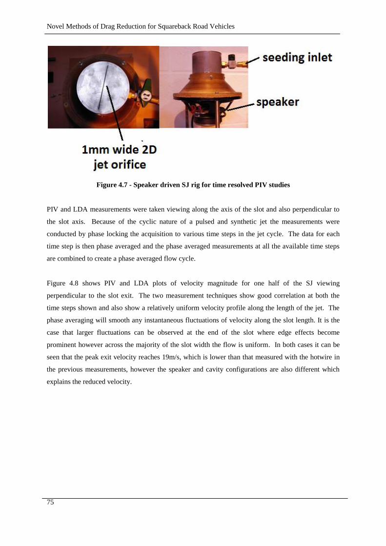
Novel Methods of Drag Reduction for Squareback Road Vehicles
75
Figure 4.7 - Speaker driven SJ rig for time resolved PIV studies
PIV and LDA measurements were taken viewing along the axis of the slot and also perpendicular to
the slot axis. Because of the cyclic nature of a pulsed and synthetic jet the measurements were
conducted by phase locking the acquisition to various time steps in the jet cycle. The data for each
time step is then phase averaged and the phase averaged measurements at all the available time steps
are combined to create a phase averaged flow cycle.
Figure 4.8 shows PIV and LDA plots of velocity magnitude for one half of the SJ viewing
perpendicular to the slot exit. The two measurement techniques show good correlation at both the
time steps shown and also show a relatively uniform velocity profile along the length of the jet. The
phase averaging will smooth any instantaneous fluctuations of velocity along the slot length. It is the
case that larger fluctuations can be observed at the end of the slot where edge effects become
prominent however across the majority of the slot width the flow is uniform. In both cases it can be
seen that the peak exit velocity reaches 19m/s, which is lower than that measured with the hotwire in
the previous measurements, however the speaker and cavity configurations are also different which
explains the reduced velocity.
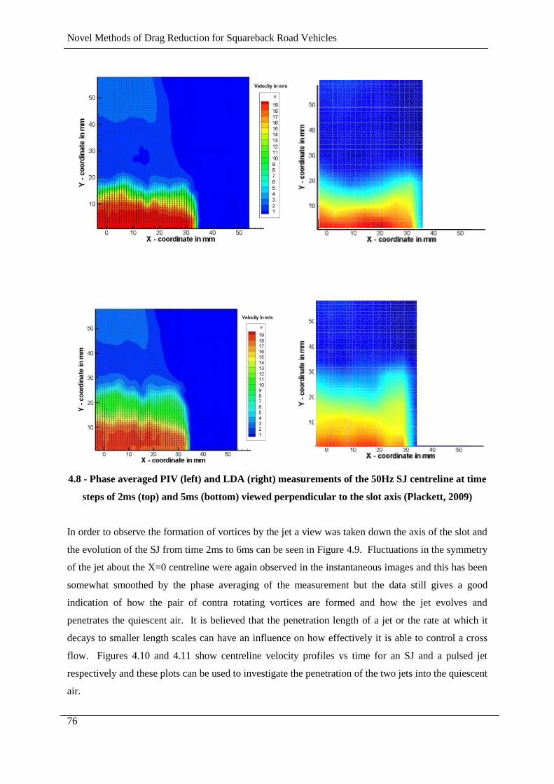
Novel Methods of Drag Reduction for Squareback Road Vehicles
76
4.8 - Phase averaged PIV (left) and LDA (right) measurements of the 50Hz SJ centreline at time
steps of 2ms (top) and 5ms (bottom) viewed perpendicular to the slot axis (Plackett, 2009)
In order to observe the formation of vortices by the jet a view was taken down the axis of the slot and
the evolution of the SJ from time 2ms to 6ms can be seen in Figure 4.9. Fluctuations in the symmetry
of the jet about the X=0 centreline were again observed in the instantaneous images and this has been
somewhat smoothed by the phase averaging of the measurement but the data still gives a good
indication of how the pair of contra rotating vortices are formed and how the jet evolves and
penetrates the quiescent air. It is believed that the penetration length of a jet or the rate at which it
decays to smaller length scales can have an influence on how effectively it is able to control a cross
flow. Figures 4.10 and 4.11 show centreline velocity profiles vs time for an SJ and a pulsed jet
respectively and these plots can be used to investigate the penetration of the two jets into the quiescent
air.
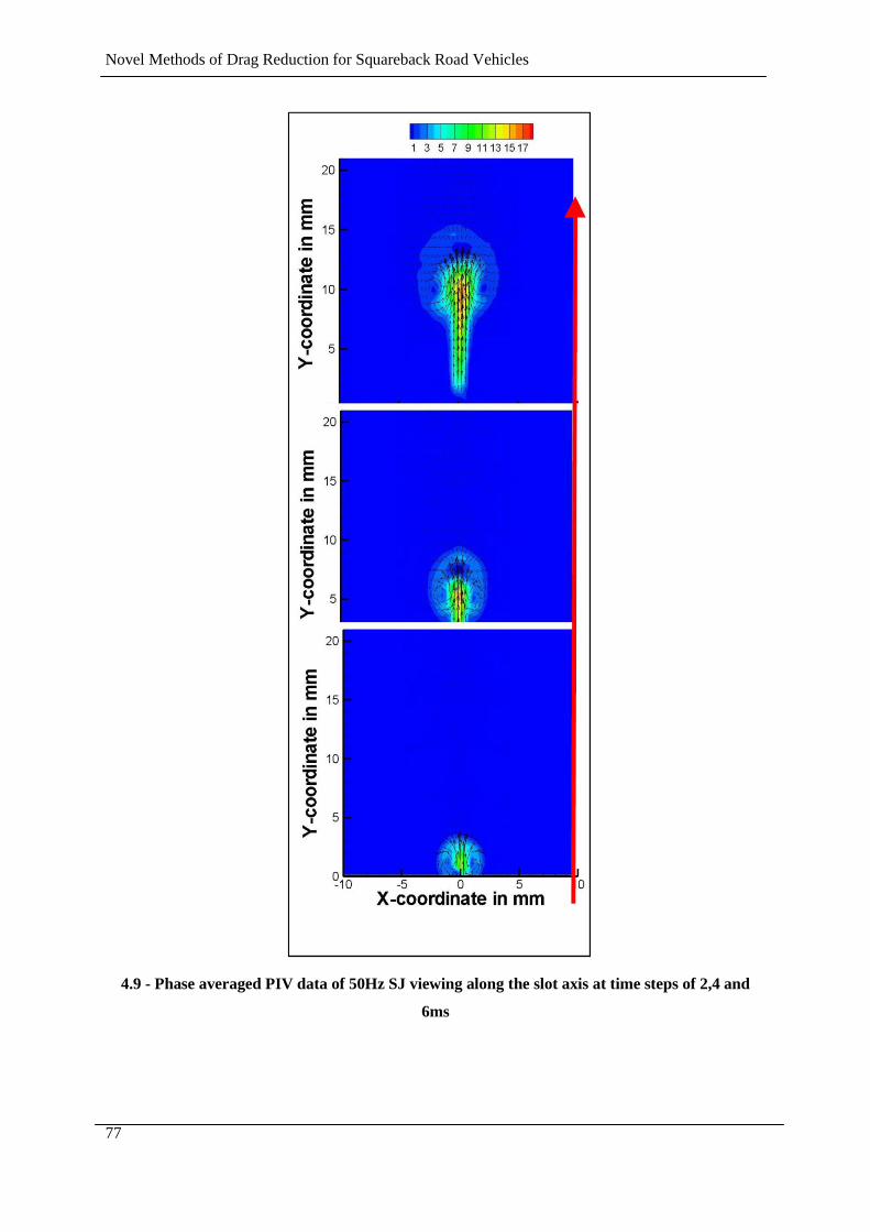
Novel Methods of Drag Reduction for Squareback Road Vehicles
77
4.9 - Phase averaged PIV data of 50Hz SJ viewing along the slot axis at time steps of 2,4 and
6ms
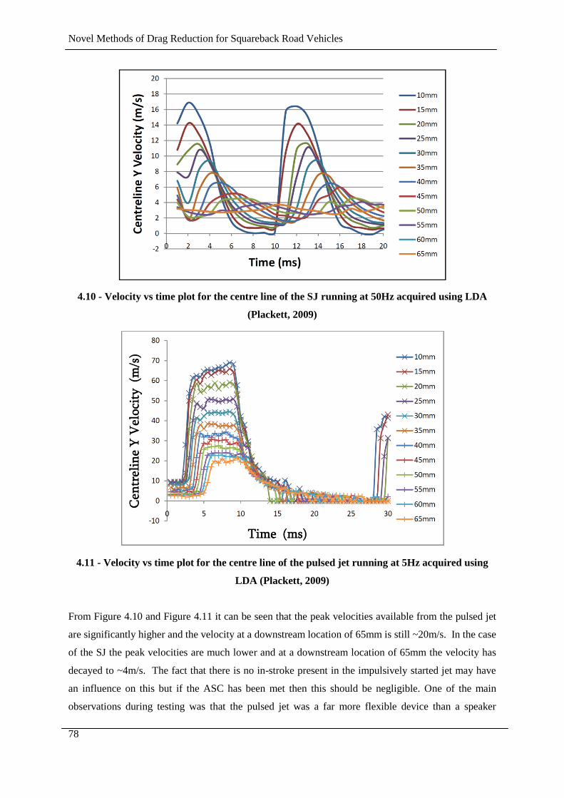
Novel Methods of Drag Reduction for Squareback Road Vehicles
78
4.10 - Velocity vs time plot for the centre line of the SJ running at 50Hz acquired using LDA
(Plackett, 2009)
4.11 - Velocity vs time plot for the centre line of the pulsed jet running at 5Hz acquired using
LDA (Plackett, 2009)
From Figure 4.10 and Figure 4.11 it can be seen that the peak velocities available from the pulsed jet
are significantly higher and the velocity at a downstream location of 65mm is still ~20m/s. In the case
of the SJ the peak velocities are much lower and at a downstream location of 65mm the velocity has
decayed to ~4m/s. The fact that there is no in-stroke present in the impulsively started jet may have
an influence on this but if the ASC has been met then this should be negligible. One of the main
observations during testing was that the pulsed jet was a far more flexible device than a speaker
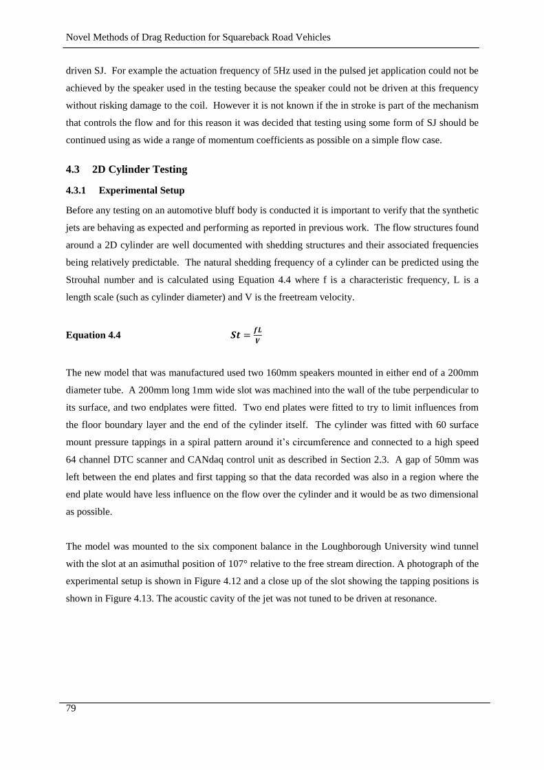
Novel Methods of Drag Reduction for Squareback Road Vehicles
79
driven SJ. For example the actuation frequency of 5Hz used in the pulsed jet application could not be
achieved by the speaker used in the testing because the speaker could not be driven at this frequency
without risking damage to the coil. However it is not known if the in stroke is part of the mechanism
that controls the flow and for this reason it was decided that testing using some form of SJ should be
continued using as wide a range of momentum coefficients as possible on a simple flow case.
4.3 2D Cylinder Testing
4.3.1 Experimental Setup
Before any testing on an automotive bluff body is conducted it is important to verify that the synthetic
jets are behaving as expected and performing as reported in previous work. The flow structures found
around a 2D cylinder are well documented with shedding structures and their associated frequencies
being relatively predictable. The natural shedding frequency of a cylinder can be predicted using the
Strouhal number and is calculated using Equation 4.4 where f is a characteristic frequency, L is a
length scale (such as cylinder diameter) and V is the freetream velocity.
Equation 4.4
The new model that was manufactured used two 160mm speakers mounted in either end of a 200mm
diameter tube. A 200mm long 1mm wide slot was machined into the wall of the tube perpendicular to
its surface, and two endplates were fitted. Two end plates were fitted to try to limit influences from
the floor boundary layer and the end of the cylinder itself. The cylinder was fitted with 60 surface
mount pressure tappings in a spiral pattern around it’s circumference and connected to a high speed
64 channel DTC scanner and CANdaq control unit as described in Section 2.3. A gap of 50mm was
left between the end plates and first tapping so that the data recorded was also in a region where the
end plate would have less influence on the flow over the cylinder and it would be as two dimensional
as possible.
The model was mounted to the six component balance in the Loughborough University wind tunnel
with the slot at an asimuthal position of 107° relative to the free stream direction. A photograph of the
experimental setup is shown in Figure 4.12 and a close up of the slot showing the tapping positions is
shown in Figure 4.13. The acoustic cavity of the jet was not tuned to be driven at resonance.
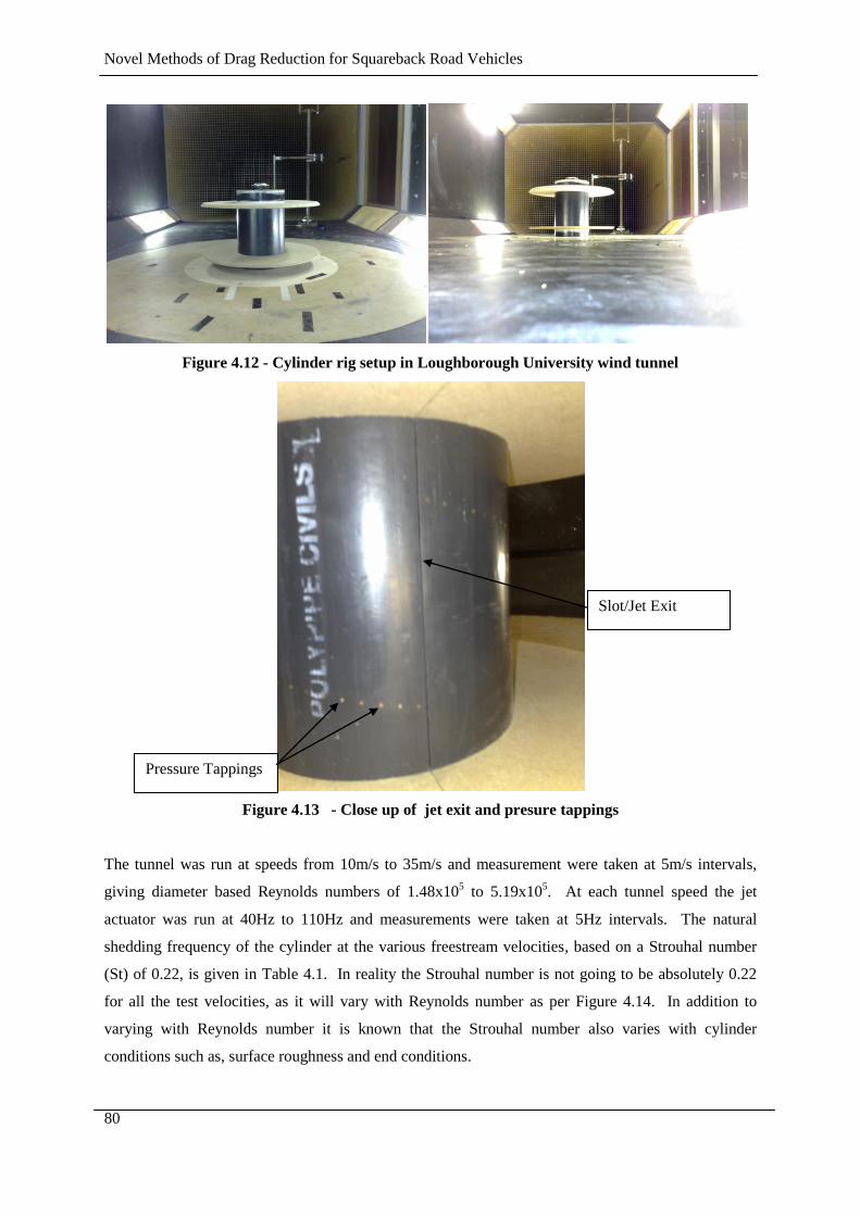
Novel Methods of Drag Reduction for Squareback Road Vehicles
80
Figure 4.12 - Cylinder rig setup in Loughborough University wind tunnel
Figure 4.13 - Close up of jet exit and presure tappings
The tunnel was run at speeds from 10m/s to 35m/s and measurement were taken at 5m/s intervals,
giving diameter based Reynolds numbers of 1.48x10⁵ to 5.19x10
5. At each tunnel speed the jet
actuator was run at 40Hz to 110Hz and measurements were taken at 5Hz intervals. The natural
shedding frequency of the cylinder at the various freestream velocities, based on a Strouhal number
(St) of 0.22, is given in Table 4.1. In reality the Strouhal number is not going to be absolutely 0.22
for all the test velocities, as it will vary with Reynolds number as per Figure 4.14. In addition to
varying with Reynolds number it is known that the Strouhal number also varies with cylinder
conditions such as, surface roughness and end conditions.
Pressure Tappings
Slot/Jet Exit
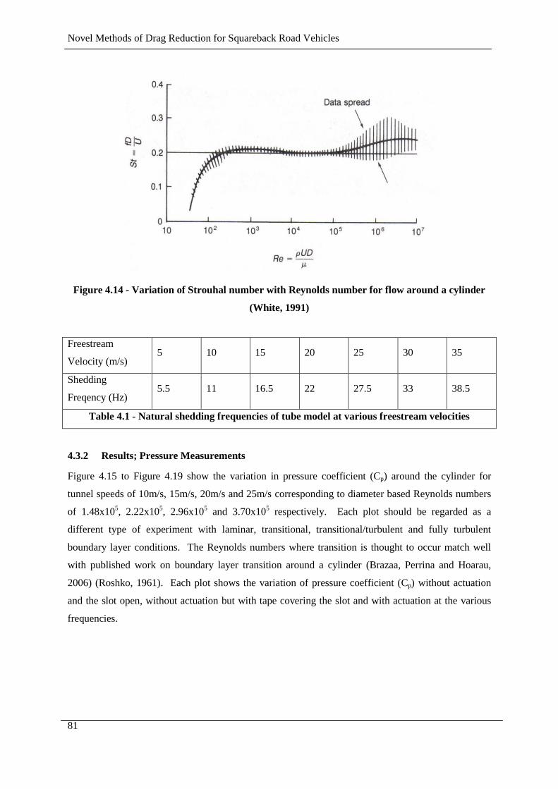
Novel Methods of Drag Reduction for Squareback Road Vehicles
81
Figure 4.14 - Variation of Strouhal number with Reynolds number for flow around a cylinder
(White, 1991)
Freestream
Velocity (m/s) 5 10 15 20 25 30 35
Shedding
Freqency (Hz) 5.5 11 16.5 22 27.5 33 38.5
Table 4.1 - Natural shedding frequencies of tube model at various freestream velocities
4.3.2 Results; Pressure Measurements
Figure 4.15 to Figure 4.19 show the variation in pressure coefficient (Cp) around the cylinder for
tunnel speeds of 10m/s, 15m/s, 20m/s and 25m/s corresponding to diameter based Reynolds numbers
of 1.48x10⁵, 2.22x10
5, 2.96x10
5 and 3.70x10
5 respectively. Each plot should be regarded as a
different type of experiment with laminar, transitional, transitional/turbulent and fully turbulent
boundary layer conditions. The Reynolds numbers where transition is thought to occur match well
with published work on boundary layer transition around a cylinder (Brazaa, Perrina and Hoarau,
2006) (Roshko, 1961). Each plot shows the variation of pressure coefficient (Cp) without actuation
and the slot open, without actuation but with tape covering the slot and with actuation at the various
frequencies.
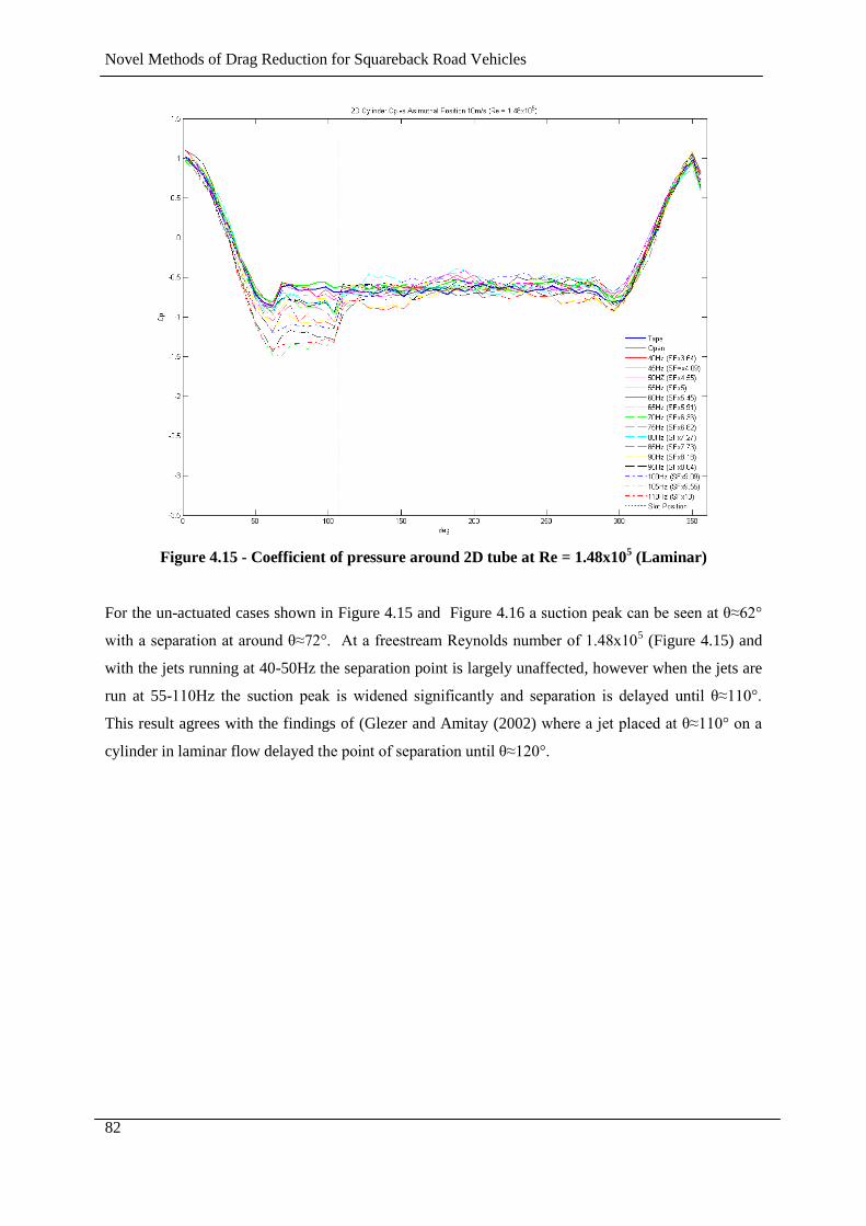
Novel Methods of Drag Reduction for Squareback Road Vehicles
82
Figure 4.15 - Coefficient of pressure around 2D tube at Re = 1.48x10⁵ (Laminar)
For the un-actuated cases shown in Figure 4.15 and Figure 4.16 a suction peak can be seen at θ≈62°
with a separation at around θ≈72°. At a freestream Reynolds number of 1.48x10⁵ (Figure 4.15) and
with the jets running at 40-50Hz the separation point is largely unaffected, however when the jets are
run at 55-110Hz the suction peak is widened significantly and separation is delayed until θ≈110°.
This result agrees with the findings of (Glezer and Amitay (2002) where a jet placed at θ≈110° on a
cylinder in laminar flow delayed the point of separation until θ≈120°.
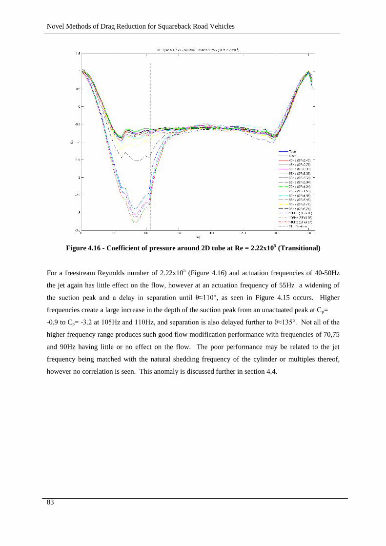
Novel Methods of Drag Reduction for Squareback Road Vehicles
83
Figure 4.16 - Coefficient of pressure around 2D tube at Re = 2.22x10⁵ (Transitional)
For a freestream Reynolds number of 2.22x10⁵ (Figure 4.16) and actuation frequencies of 40-50Hz
the jet again has little effect on the flow, however at an actuation frequency of 55Hz a widening of
the suction peak and a delay in separation until θ≈110°, as seen in Figure 4.15 occurs. Higher
frequencies create a large increase in the depth of the suction peak from an unactuated peak at Cp=
-0.9 to Cp= -3.2 at 105Hz and 110Hz, and separation is also delayed further to θ≈135°. Not all of the
higher frequency range produces such good flow modification performance with frequencies of 70,75
and 90Hz having little or no effect on the flow. The poor performance may be related to the jet
frequency being matched with the natural shedding frequency of the cylinder or multiples thereof,
however no correlation is seen. This anomaly is discussed further in section 4.4.
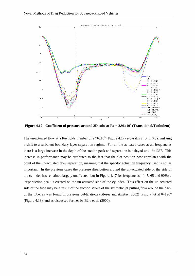
Novel Methods of Drag Reduction for Squareback Road Vehicles
84
Figure 4.17 - Coefficient of pressure around 2D tube at Re = 2.96x10⁵ (Transitional/Turbulent)
The un-actuated flow at a Reynolds number of 2.96x10⁵ (Figure 4.17) separates at θ≈110°, signifying
a shift to a turbulent boundary layer separation regime. For all the actuated cases at all frequencies
there is a large increase in the depth of the suction peak and separation is delayed until θ≈135°. This
increase in performance may be attributed to the fact that the slot position now correlates with the
point of the un-actuated flow separation, meaning that the specific actuation frequency used is not as
important. In the previous cases the pressure distribution around the un-actuated side of the side of
the cylinder has remained largely unaffected, but in Figure 4.17 for frequencies of 45, 65 and 90Hz a
large suction peak is created on the un-actuated side of the cylinder. This effect on the un-actuated
side of the tube may be a result of the suction stroke of the synthetic jet pulling flow around the back
of the tube, as was found in previous publications (Glezer and Amitay, 2002) using a jet at θ≈120°
(Figure 4.18), and as discussed further by Béra et al. (2000).

Novel Methods of Drag Reduction for Squareback Road Vehicles
85
Figure 4.18- Variations of Cp on a tube with a synthetic jet at θ=120°
( ○) baseline and (●) actuated (Glezer and Amitay, 2002)
Figure 4.19 - Coefficient of pressure around 2D tube at Re = 3.70x10⁵ (Fully Turbulent)
For a Reynolds number of 3.70x10⁵ (Figure 4.19) the un-actuated flows display a very clear turbulent
separation at θ≈110°. When the synthetic jet is running none of the actuation frequencies displace the
separation point further around the tube as found in Figure 4.16 and Figure 4.17. While it is possible
that this result demonstrates that the synthetic jets are not effective at higher Reynolds numbers it may
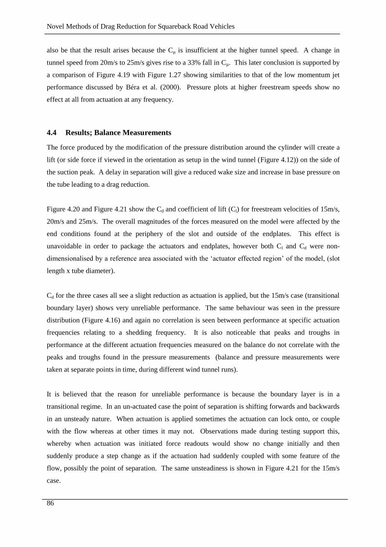
Novel Methods of Drag Reduction for Squareback Road Vehicles
86
also be that the result arises because the Cµ is insufficient at the higher tunnel speed. A change in
tunnel speed from 20m/s to 25m/s gives rise to a 33% fall in Cµ. This later conclusion is supported by
a comparison of Figure 4.19 with Figure 1.27 showing similarities to that of the low momentum jet
performance discussed by Béra et al. (2000). Pressure plots at higher freestream speeds show no
effect at all from actuation at any frequency.
4.4 Results; Balance Measurements
The force produced by the modification of the pressure distribution around the cylinder will create a
lift (or side force if viewed in the orientation as setup in the wind tunnel (Figure 4.12)) on the side of
the suction peak. A delay in separation will give a reduced wake size and increase in base pressure on
the tube leading to a drag reduction.
Figure 4.20 and Figure 4.21 show the Cd and coefficient of lift (Cl) for freestream velocities of 15m/s,
20m/s and 25m/s. The overall magnitudes of the forces measured on the model were affected by the
end conditions found at the periphery of the slot and outside of the endplates. This effect is
unavoidable in order to package the actuators and endplates, however both Cl and Cd were non-
dimensionalised by a reference area associated with the ‘actuator effected region’ of the model, (slot
length x tube diameter).
Cd for the three cases all see a slight reduction as actuation is applied, but the 15m/s case (transitional
boundary layer) shows very unreliable performance. The same behaviour was seen in the pressure
distribution (Figure 4.16) and again no correlation is seen between performance at specific actuation
frequencies relating to a shedding frequency. It is also noticeable that peaks and troughs in
performance at the different actuation frequencies measured on the balance do not correlate with the
peaks and troughs found in the pressure measurements (balance and pressure measurements were
taken at separate points in time, during different wind tunnel runs).
It is believed that the reason for unreliable performance is because the boundary layer is in a
transitional regime. In an un-actuated case the point of separation is shifting forwards and backwards
in an unsteady nature. When actuation is applied sometimes the actuation can lock onto, or couple
with the flow whereas at other times it may not. Observations made during testing support this,
whereby when actuation was initiated force readouts would show no change initially and then
suddenly produce a step change as if the actuation had suddenly coupled with some feature of the
flow, possibly the point of separation. The same unsteadiness is shown in Figure 4.21 for the 15m/s
case.
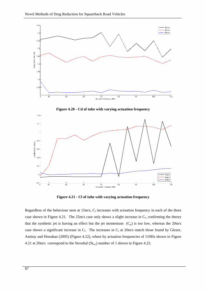
Novel Methods of Drag Reduction for Squareback Road Vehicles
87
Figure 4.20 - Cd of tube with varying actuation frequency
Figure 4.21 - Cl of tube with varying actuation frequency
Regardless of the behaviour seen at 15m/s, Cl increases with actuation frequency in each of the three
case shown in Figure 4.21. The 25m/s case only shows a slight increase in Cl, confirming the theory
that the synthetic jet is having an effect but the jet momentum (Cµ) is too low, whereas the 20m/s
case shows a significant increase in Cl. The increases in Cl at 20m/s match those found by Glezer,
Amitay and Honahan (2005) (Figure 4.22), where by actuation frequencies of 110Hz shown in Figure
4.21 at 20m/s correspond to the Strouhal (Stact) number of 1 shown in Figure 4.22.
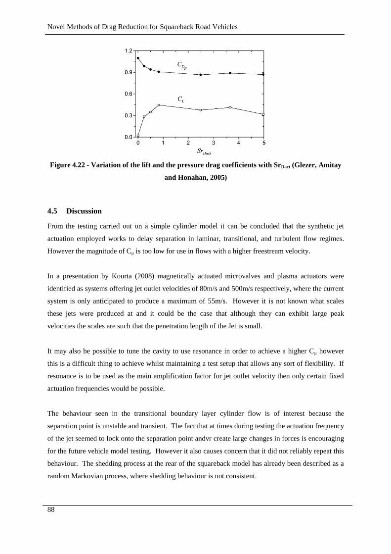
Novel Methods of Drag Reduction for Squareback Road Vehicles
88
Figure 4.22 - Variation of the lift and the pressure drag coefficients with SrDact (Glezer, Amitay
and Honahan, 2005)
4.5 Discussion
From the testing carried out on a simple cylinder model it can be concluded that the synthetic jet
actuation employed works to delay separation in laminar, transitional, and turbulent flow regimes.
However the magnitude of Cµ is too low for use in flows with a higher freestream velocity.
In a presentation by Kourta (2008) magnetically actuated microvalves and plasma actuators were
identified as systems offering jet outlet velocities of 80m/s and 500m/s respectively, where the current
system is only anticipated to produce a maximum of 55m/s. However it is not known what scales
these jets were produced at and it could be the case that although they can exhibit large peak
velocities the scales are such that the penetration length of the Jet is small.
It may also be possible to tune the cavity to use resonance in order to achieve a higher Cµ however
this is a difficult thing to achieve whilst maintaining a test setup that allows any sort of flexibility. If
resonance is to be used as the main amplification factor for jet outlet velocity then only certain fixed
actuation frequencies would be possible.
The behaviour seen in the transitional boundary layer cylinder flow is of interest because the
separation point is unstable and transient. The fact that at times during testing the actuation frequency
of the jet seemed to lock onto the separation point andvr create large changes in forces is encouraging
for the future vehicle model testing. However it also causes concern that it did not reliably repeat this
behaviour. The shedding process at the rear of the squareback model has already been described as a
random Markovian process, where shedding behaviour is not consistent.
Novel Methods of Drag Reduction for Squareback Road Vehicles
89
The difficulties in creating a large momentum coefficient and the concerns about the repeatability of
success with synthetic jets, means that the probability of an experiment combining synthetic jets and a
vehicle model being successful is significantly reduced.
The current testing has also highlighted the constraints associated with using acoustic drives to
generate jets. If the jet is designed to run at resonance this restricts the operating frequencies to one or
two choices, that may not be matched to the required frequency to control cross flow. The speakers
that have been used also normally have a minimum drive frequency that they can be run at before the
coil is damaged. This also restricts the lower frequency ranges available that may be of interest.
In the current testing the impulsively driven jets demonstrated that they can be operated with a great
deal of flexibility and actuated at almost any frequency required. The use of a pressurised air source
may not be desirable for the final application to road vehicles but in the context of experimental
investigations seem to offer the most flexibility. In the first application of jets to control flow around
the more complex Windsor model it was decided to simplify the actuators to allow greater control of
the experiment. For this reason the first tests were conducted using steady blowing
Novel Methods of Drag Reduction for Squareback Road Vehicles
90
Chapter 5
ACTIVE CONTROL - CONSTANT BLOWING
EXPERIMENTS, RESULTS AND DISCUSSION
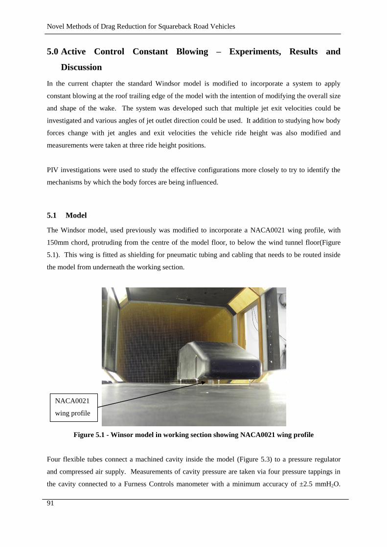
Novel Methods of Drag Reduction for Squareback Road Vehicles
91
5.0 Active Control Constant Blowing – Experiments, Results and
Discussion
In the current chapter the standard Windsor model is modified to incorporate a system to apply
constant blowing at the roof trailing edge of the model with the intention of modifying the overall size
and shape of the wake. The system was developed such that multiple jet exit velocities could be
investigated and various angles of jet outlet direction could be used. It addition to studying how body
forces change with jet angles and exit velocities the vehicle ride height was also modified and
measurements were taken at three ride height positions.
PIV investigations were used to study the effective configurations more closely to try to identify the
mechanisms by which the body forces are being influenced.
5.1 Model
The Windsor model, used previously was modified to incorporate a NACA0021 wing profile, with
150mm chord, protruding from the centre of the model floor, to below the wind tunnel floor(Figure
5.1). This wing is fitted as shielding for pneumatic tubing and cabling that needs to be routed inside
the model from underneath the working section.
Figure 5.1 - Winsor model in working section showing NACA0021 wing profile
Four flexible tubes connect a machined cavity inside the model (Figure 5.3) to a pressure regulator
and compressed air supply. Measurements of cavity pressure are taken via four pressure tappings in
the cavity connected to a Furness Controls manometer with a minimum accuracy of ±2.5 mmH2O.
NACA0021
wing profile
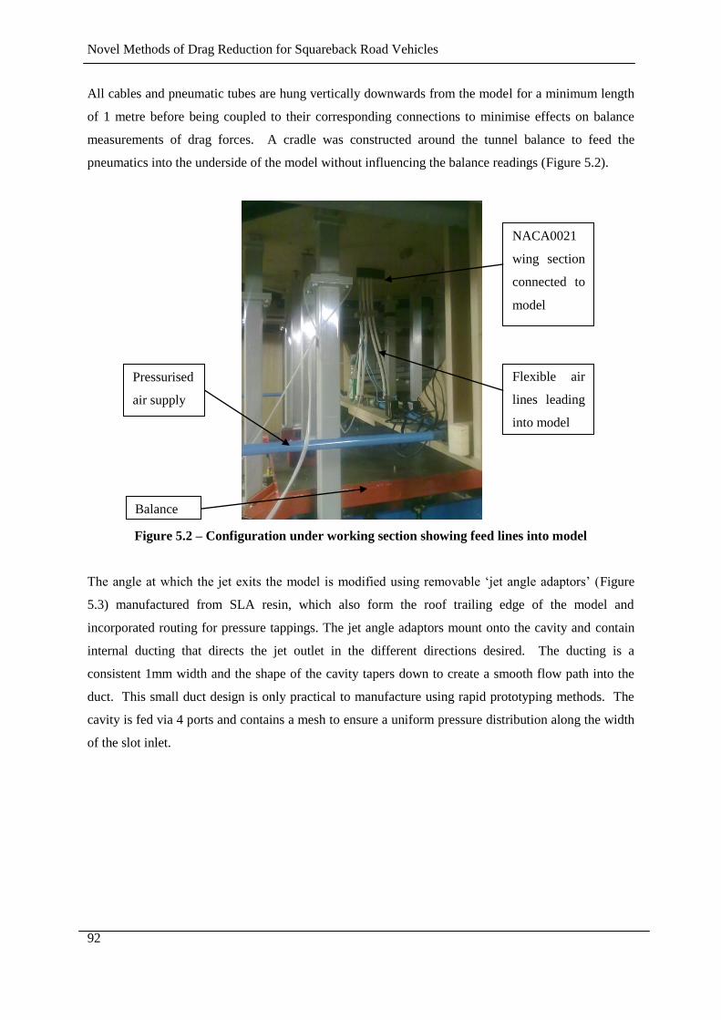
Novel Methods of Drag Reduction for Squareback Road Vehicles
92
All cables and pneumatic tubes are hung vertically downwards from the model for a minimum length
of 1 metre before being coupled to their corresponding connections to minimise effects on balance
measurements of drag forces. A cradle was constructed around the tunnel balance to feed the
pneumatics into the underside of the model without influencing the balance readings (Figure 5.2).
Figure 5.2 – Configuration under working section showing feed lines into model
The angle at which the jet exits the model is modified using removable ‘jet angle adaptors’ (Figure
5.3) manufactured from SLA resin, which also form the roof trailing edge of the model and
incorporated routing for pressure tappings. The jet angle adaptors mount onto the cavity and contain
internal ducting that directs the jet outlet in the different directions desired. The ducting is a
consistent 1mm width and the shape of the cavity tapers down to create a smooth flow path into the
duct. This small duct design is only practical to manufacture using rapid prototyping methods. The
cavity is fed via 4 ports and contains a mesh to ensure a uniform pressure distribution along the width
of the slot inlet.
Balance
Pressurised
air supply
Flexible air
lines leading
into model
NACA0021
wing section
connected to
model
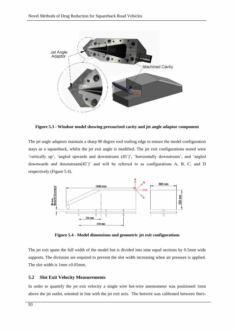
Novel Methods of Drag Reduction for Squareback Road Vehicles
93
Figure 5.3 - Windsor model showing pressurised cavity and jet angle adaptor component
The jet angle adaptors maintain a sharp 90 degree roof trailing edge to ensure the model configuration
stays as a squareback, whilst the jet exit angle is modified. The jet exit configurations tested were
‘vertically up’, ‘angled upwards and downstream (45˚)’, ‘horizontally downstream’, and ‘angled
downwards and downstream(45˚)’ and will be referred to as configurations A, B, C, and D
respectively (Figure 5.4).
Figure 5.4 - Model dimensions and geometric jet exit configurations
The jet exit spans the full width of the model but is divided into nine equal sections by 0.5mm wide
supports. The divisions are required to prevent the slot width increasing when air pressure is applied.
The slot width is 1mm ±0.05mm.
5.2 Slot Exit Velocity Measurements
In order to quantify the jet exit velocity a single wire hot-wire anemometer was positioned 1mm
above the jet outlet, oriented in line with the jet exit axis. The hotwire was calibrated between 0m/s-
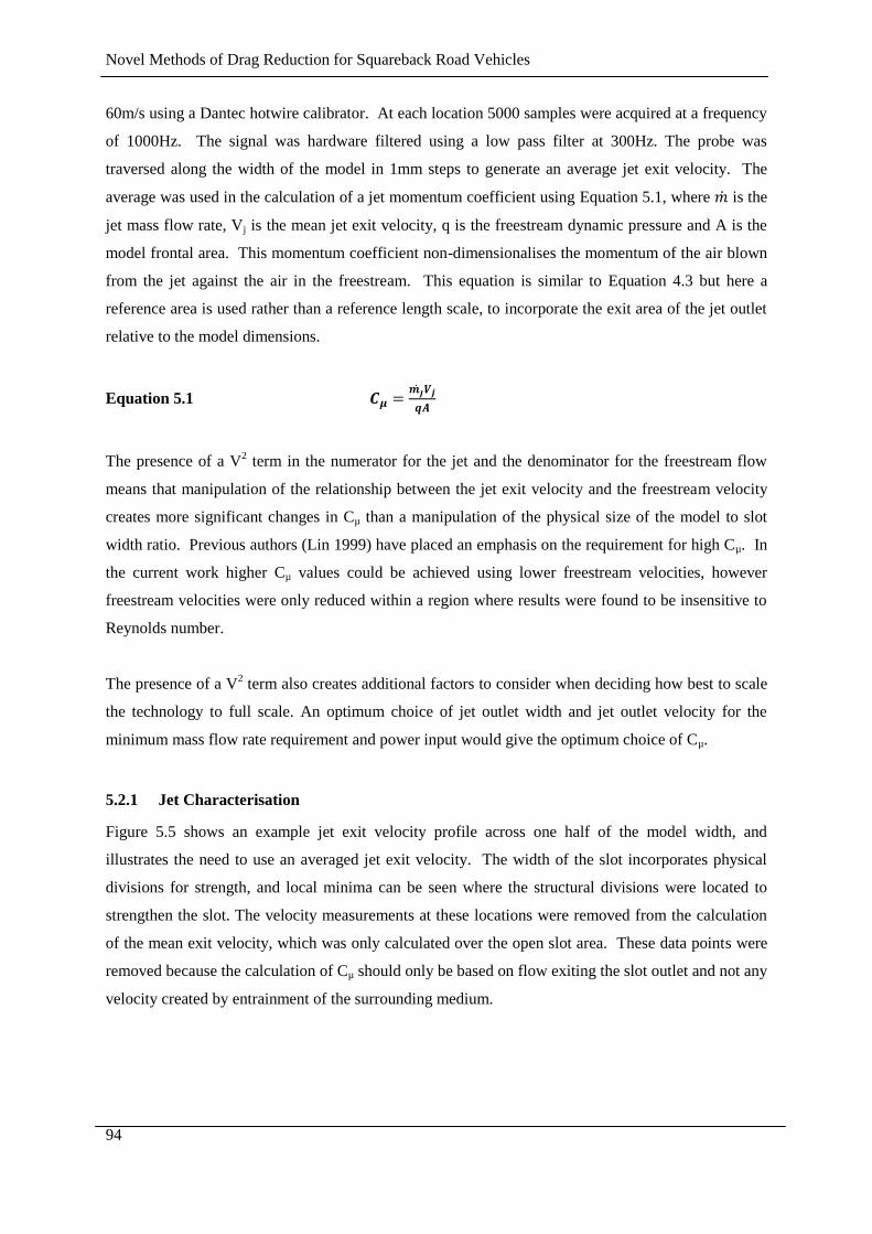
Novel Methods of Drag Reduction for Squareback Road Vehicles
94
60m/s using a Dantec hotwire calibrator. At each location 5000 samples were acquired at a frequency
of 1000Hz. The signal was hardware filtered using a low pass filter at 300Hz. The probe was
traversed along the width of the model in 1mm steps to generate an average jet exit velocity. The
average was used in the calculation of a jet momentum coefficient using Equation 5.1, where is the
jet mass flow rate, Vj is the mean jet exit velocity, q is the freestream dynamic pressure and A is the
model frontal area. This momentum coefficient non-dimensionalises the momentum of the air blown
from the jet against the air in the freestream. This equation is similar to Equation 4.3 but here a
reference area is used rather than a reference length scale, to incorporate the exit area of the jet outlet
relative to the model dimensions.
Equation 5.1
The presence of a V2 term in the numerator for the jet and the denominator for the freestream flow
means that manipulation of the relationship between the jet exit velocity and the freestream velocity
creates more significant changes in Cµ than a manipulation of the physical size of the model to slot
width ratio. Previous authors (Lin 1999) have placed an emphasis on the requirement for high Cµ. In
the current work higher Cµ values could be achieved using lower freestream velocities, however
freestream velocities were only reduced within a region where results were found to be insensitive to
Reynolds number.
The presence of a V2 term also creates additional factors to consider when deciding how best to scale
the technology to full scale. An optimum choice of jet outlet width and jet outlet velocity for the
minimum mass flow rate requirement and power input would give the optimum choice of Cµ.
5.2.1 Jet Characterisation
Figure 5.5 shows an example jet exit velocity profile across one half of the model width, and
illustrates the need to use an averaged jet exit velocity. The width of the slot incorporates physical
divisions for strength, and local minima can be seen where the structural divisions were located to
strengthen the slot. The velocity measurements at these locations were removed from the calculation
of the mean exit velocity, which was only calculated over the open slot area. These data points were
removed because the calculation of Cµ should only be based on flow exiting the slot outlet and not any
velocity created by entrainment of the surrounding medium.
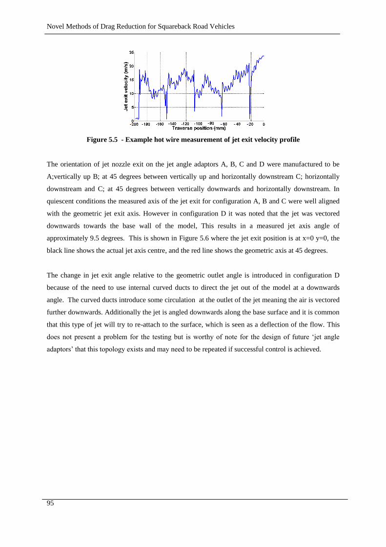
Novel Methods of Drag Reduction for Squareback Road Vehicles
95
Figure 5.5 - Example hot wire measurement of jet exit velocity profile
The orientation of jet nozzle exit on the jet angle adaptors A, B, C and D were manufactured to be
A;vertically up B; at 45 degrees between vertically up and horizontally downstream C; horizontally
downstream and C; at 45 degrees between vertically downwards and horizontally downstream. In
quiescent conditions the measured axis of the jet exit for configuration A, B and C were well aligned
with the geometric jet exit axis. However in configuration D it was noted that the jet was vectored
downwards towards the base wall of the model, This results in a measured jet axis angle of
approximately 9.5 degrees. This is shown in Figure 5.6 where the jet exit position is at x=0 y=0, the
black line shows the actual jet axis centre, and the red line shows the geometric axis at 45 degrees.
The change in jet exit angle relative to the geometric outlet angle is introduced in configuration D
because of the need to use internal curved ducts to direct the jet out of the model at a downwards
angle. The curved ducts introduce some circulation at the outlet of the jet meaning the air is vectored
further downwards. Additionally the jet is angled downwards along the base surface and it is common
that this type of jet will try to re-attach to the surface, which is seen as a deflection of the flow. This
does not present a problem for the testing but is worthy of note for the design of future ‘jet angle
adaptors’ that this topology exists and may need to be repeated if successful control is achieved.
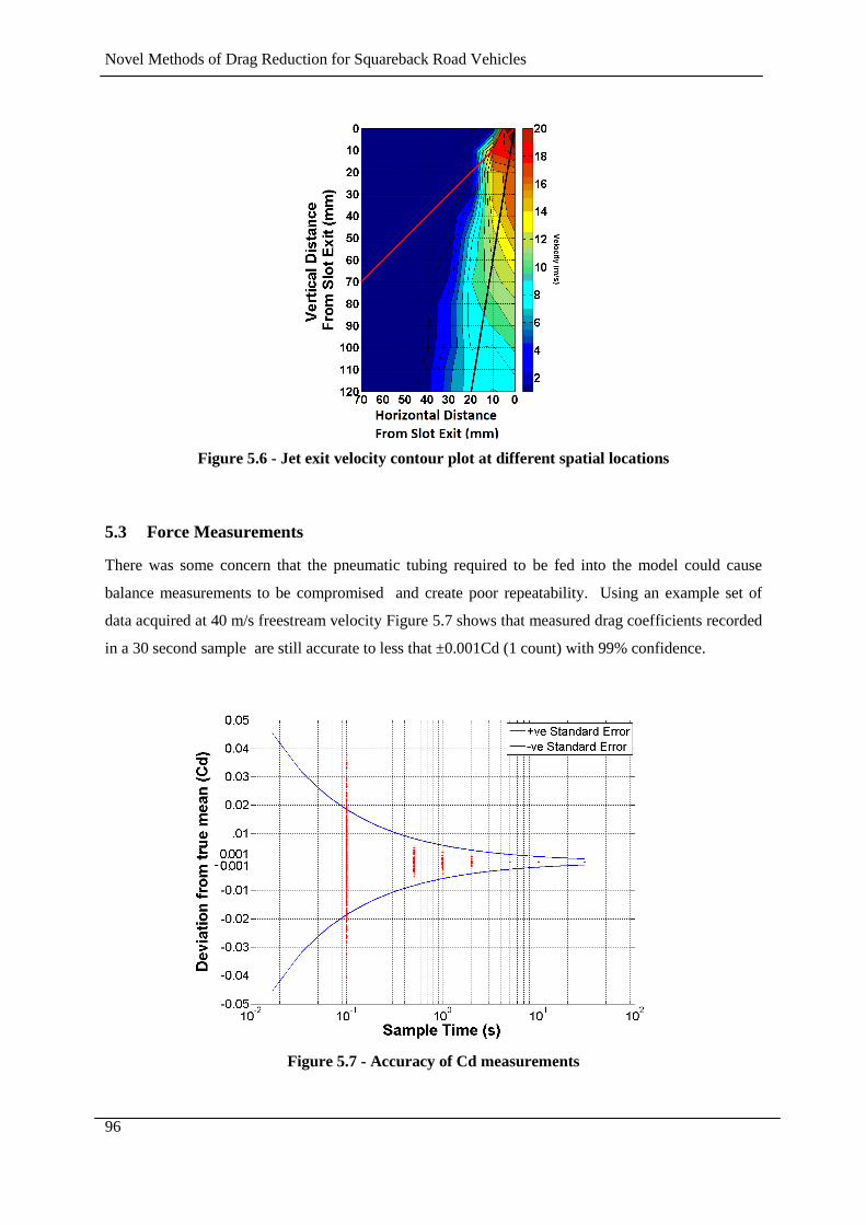
Novel Methods of Drag Reduction for Squareback Road Vehicles
96
Figure 5.6 - Jet exit velocity contour plot at different spatial locations
5.3 Force Measurements
There was some concern that the pneumatic tubing required to be fed into the model could cause
balance measurements to be compromised and create poor repeatability. Using an example set of
data acquired at 40 m/s freestream velocity Figure 5.7 shows that measured drag coefficients recorded
in a 30 second sample are still accurate to less that ±0.001Cd (1 count) with 99% confidence.
Figure 5.7 - Accuracy of Cd measurements
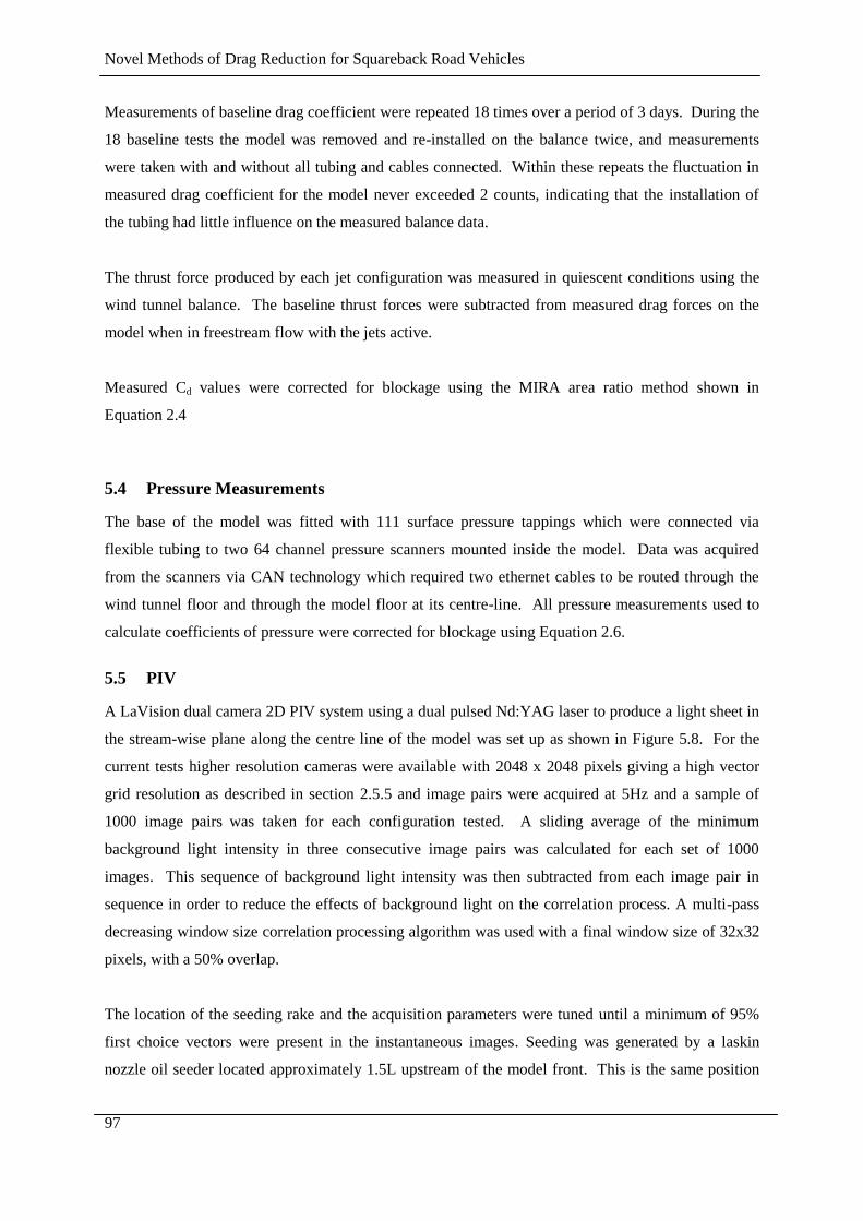
Novel Methods of Drag Reduction for Squareback Road Vehicles
97
Measurements of baseline drag coefficient were repeated 18 times over a period of 3 days. During the
18 baseline tests the model was removed and re-installed on the balance twice, and measurements
were taken with and without all tubing and cables connected. Within these repeats the fluctuation in
measured drag coefficient for the model never exceeded 2 counts, indicating that the installation of
the tubing had little influence on the measured balance data.
The thrust force produced by each jet configuration was measured in quiescent conditions using the
wind tunnel balance. The baseline thrust forces were subtracted from measured drag forces on the
model when in freestream flow with the jets active.
Measured Cd values were corrected for blockage using the MIRA area ratio method shown in
Equation 2.4
5.4 Pressure Measurements
The base of the model was fitted with 111 surface pressure tappings which were connected via
flexible tubing to two 64 channel pressure scanners mounted inside the model. Data was acquired
from the scanners via CAN technology which required two ethernet cables to be routed through the
wind tunnel floor and through the model floor at its centre-line. All pressure measurements used to
calculate coefficients of pressure were corrected for blockage using Equation 2.6.
5.5 PIV
A LaVision dual camera 2D PIV system using a dual pulsed Nd:YAG laser to produce a light sheet in
the stream-wise plane along the centre line of the model was set up as shown in Figure 5.8. For the
current tests higher resolution cameras were available with 2048 x 2048 pixels giving a high vector
grid resolution as described in section 2.5.5 and image pairs were acquired at 5Hz and a sample of
1000 image pairs was taken for each configuration tested. A sliding average of the minimum
background light intensity in three consecutive image pairs was calculated for each set of 1000
images. This sequence of background light intensity was then subtracted from each image pair in
sequence in order to reduce the effects of background light on the correlation process. A multi-pass
decreasing window size correlation processing algorithm was used with a final window size of 32x32
pixels, with a 50% overlap.
The location of the seeding rake and the acquisition parameters were tuned until a minimum of 95%
first choice vectors were present in the instantaneous images. Seeding was generated by a laskin
nozzle oil seeder located approximately 1.5L upstream of the model front. This is the same position
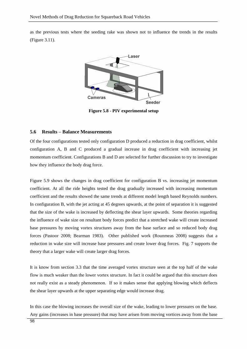
Novel Methods of Drag Reduction for Squareback Road Vehicles
98
as the previous tests where the seeding rake was shown not to influence the trends in the results
(Figure 3.11).
Figure 5.8 - PIV experimental setup
5.6 Results – Balance Measurements
Of the four configurations tested only configuration D produced a reduction in drag coefficient, whilst
configuration A, B and C produced a gradual increase in drag coefficient with increasing jet
momentum coefficient. Configurations B and D are selected for further discussion to try to investigate
how they influence the body drag force.
Figure 5.9 shows the changes in drag coefficient for configuration B vs. increasing jet momentum
coefficient. At all the ride heights tested the drag gradually increased with increasing momentum
coefficient and the results showed the same trends at different model length based Reynolds numbers.
In configuration B, with the jet acting at 45 degrees upwards, at the point of separation it is suggested
that the size of the wake is increased by deflecting the shear layer upwards. Some theories regarding
the influence of wake size on resultant body forces predict that a stretched wake will create increased
base pressures by moving vortex structures away from the base surface and so reduced body drag
forces (Pastoor 2008; Bearman 1983). Other published work (Rounmeas 2008) suggests that a
reduction in wake size will increase base pressures and create lower drag forces. Fig. 7 supports the
theory that a larger wake will create larger drag forces.
It is know from section 3.3 that the time averaged vortex structure seen at the top half of the wake
flow is much weaker than the lower vortex structure. In fact it could be argued that this structure does
not really exist as a steady phenomenon. If so it makes sense that applying blowing which deflects
the shear layer upwards at the upper separating edge would increase drag.
In this case the blowing increases the overall size of the wake, leading to lower pressures on the base.
Any gains (increases in base pressure) that may have arisen from moving vortices away from the base
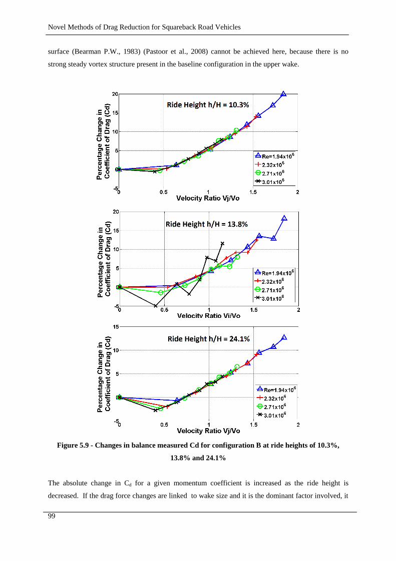
Novel Methods of Drag Reduction for Squareback Road Vehicles
99
surface (Bearman P.W., 1983) (Pastoor et al., 2008) cannot be achieved here, because there is no
strong steady vortex structure present in the baseline configuration in the upper wake.
Figure 5.9 - Changes in balance measured Cd for configuration B at ride heights of 10.3%,
13.8% and 24.1%
The absolute change in Cd for a given momentum coefficient is increased as the ride height is
decreased. If the drag force changes are linked to wake size and it is the dominant factor involved, it
Novel Methods of Drag Reduction for Squareback Road Vehicles
100
would suggest that at lower ride heights the wake size is increased more for a given momentum
coefficient. However the change in drag reduction as ride height is reduced from the extreme case of
h/H= 24.1% to h/H= 10.3% is an average of 1.7 times greater. If the change in wake size was
anything close to proportional to the changes in drag forces then the wake size increase required to
create the measured force changes would also be significant. For this reason it is believed that
additional factors within the wake have an influence on base pressures and hence body drag forces.
This would suggest that as ride height is decreased the influence of blowing on the ‘in-wake’ vortex
structures becomes more significant.
Figure 5.10 shows the changes in drag coefficient as a result of blowing using configuration D, at a
ride height of h/H = 10.3%. Significant reductions in Cd are observed which gradually increase as
momentum coefficient is increased. As seen in other configurations the trends are not sensitive to
Reynolds number, which allows larger Cµ values to be tested by reducing the freestream velocity.
Figure 5.10 - Changes in balance measured Cd for the Configuration D at a ride height of
10.3%
As per Figure 5.9 it would be reasonable to attribute the drag reductions seen in Figure 5.10 to a
deflection of the shear layer downwards creating a reduction in the overall wake size. However the
drag reductions are sufficiently large (3%-12%) that if wake size alone is the dominant influence on
base pressure and body forces the wake size reduction would be significant. The magnitudes of drag
changes observed support the theory that additional ‘in wake’ factors may have an influence on drag
forces in addition to the modification of wake size alone. In order to investigate the changes further,
base surface pressures and in wake PIV measurement techniques were used.
With Figure 5.9 and Figure 5.10 exhibiting a lack of Reynolds number sensitivity the following
sections will focus on a test Reynolds number of 3.01x10⁶ which has been chosen for further analysis.
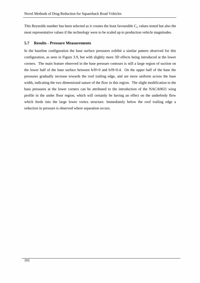
Novel Methods of Drag Reduction for Squareback Road Vehicles
101
This Reynolds number has been selected as it creates the least favourable Cµ values tested but also the
most representative values if the technology were to be scaled up to production vehicle magnitudes.
5.7 Results - Pressure Measurements
In the baseline configuration the base surface pressures exhibit a similar pattern observed for this
configuration, as seen in Figure 3.9, but with slightly more 3D effects being introduced at the lower
corners. The main feature observed in the base pressure contours is still a large region of suction on
the lower half of the base surface between h/H=0 and h/H=0.4. On the upper half of the base the
pressures gradually increase towards the roof trailing edge, and are more uniform across the base
width, indicating the two dimensional nature of the flow in this region. The slight modification to the
base pressures at the lower corners can be attributed to the introduction of the NACA0021 wing
profile in the under floor region, which will certainly be having an effect on the underbody flow
which feeds into the large lower vortex structure. Immediately below the roof trailing edge a
reduction in pressure is observed where separation occurs.

Novel Methods of Drag Reduction for Squareback Road Vehicles
102
Figure 5.11 - Base pressure contours for: a)baseline and b) blowing configuration D at Cµ =
0.013 and Re = 3.01x10⁶
When blowing is applied in Configuration D at a momentum coefficient of 0.013 a global increase in
base pressures is observed (Figure 5.11b). The pressure contour patterns observed in Figure 5.11a
remain present in Figure 5.11b however the low pressures observed in the lower half of the base for
the baseline configuration have increased with the application of blowing. This increase has resulted
in a more uniform distribution of base pressures and a less pronounced suction region between h/H=0
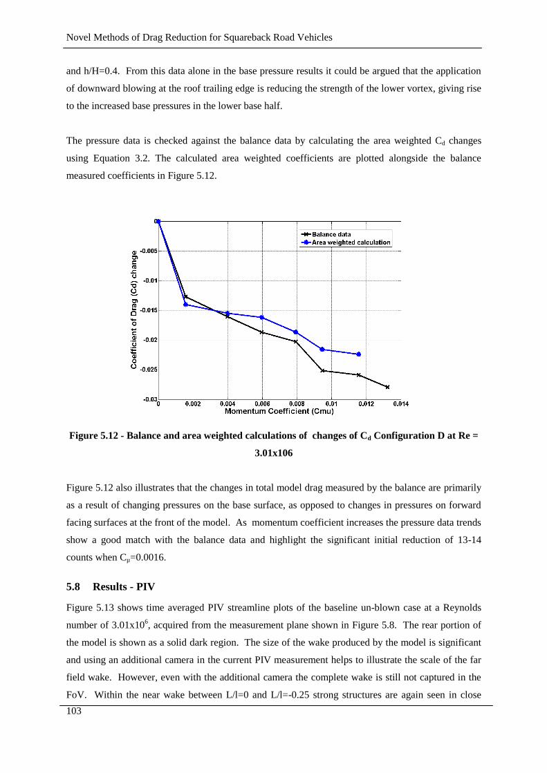
Novel Methods of Drag Reduction for Squareback Road Vehicles
103
and h/H=0.4. From this data alone in the base pressure results it could be argued that the application
of downward blowing at the roof trailing edge is reducing the strength of the lower vortex, giving rise
to the increased base pressures in the lower base half.
The pressure data is checked against the balance data by calculating the area weighted Cd changes
using Equation 3.2. The calculated area weighted coefficients are plotted alongside the balance
measured coefficients in Figure 5.12.
Figure 5.12 - Balance and area weighted calculations of changes of Cd Configuration D at Re =
3.01x10⁶
Figure 5.12 also illustrates that the changes in total model drag measured by the balance are primarily
as a result of changing pressures on the base surface, as opposed to changes in pressures on forward
facing surfaces at the front of the model. As momentum coefficient increases the pressure data trends
show a good match with the balance data and highlight the significant initial reduction of 13-14
counts when Cµ=0.0016.
5.8 Results - PIV
Figure 5.13 shows time averaged PIV streamline plots of the baseline un-blown case at a Reynolds
number of 3.01x10⁶, acquired from the measurement plane shown in Figure 5.8. The rear portion of
the model is shown as a solid dark region. The size of the wake produced by the model is significant
and using an additional camera in the current PIV measurement helps to illustrate the scale of the far
field wake. However, even with the additional camera the complete wake is still not captured in the
FoV. Within the near wake between L/l=0 and L/l=-0.25 strong structures are again seen in close
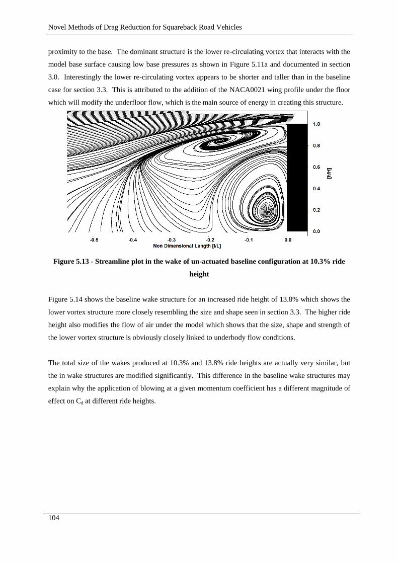
Novel Methods of Drag Reduction for Squareback Road Vehicles
104
proximity to the base. The dominant structure is the lower re-circulating vortex that interacts with the
model base surface causing low base pressures as shown in Figure 5.11a and documented in section
3.0. Interestingly the lower re-circulating vortex appears to be shorter and taller than in the baseline
case for section 3.3. This is attributed to the addition of the NACA0021 wing profile under the floor
which will modify the underfloor flow, which is the main source of energy in creating this structure.
Figure 5.13 - Streamline plot in the wake of un-actuated baseline configuration at 10.3% ride
height
Figure 5.14 shows the baseline wake structure for an increased ride height of 13.8% which shows the
lower vortex structure more closely resembling the size and shape seen in section 3.3. The higher ride
height also modifies the flow of air under the model which shows that the size, shape and strength of
the lower vortex structure is obviously closely linked to underbody flow conditions.
The total size of the wakes produced at 10.3% and 13.8% ride heights are actually very similar, but
the in wake structures are modified significantly. This difference in the baseline wake structures may
explain why the application of blowing at a given momentum coefficient has a different magnitude of
effect on Cd at different ride heights.

Novel Methods of Drag Reduction for Squareback Road Vehicles
105
Figure 5.14 - Streamline plot in the wake of un-actuated baseline configuration at 13.8% ride
height
Figure 5.15 shows the effect of steady blowing in configuration B, where streamlines that start at the
rear separating edge as seen to rise upwards and out of the FoV, indicating that the separated flow is
being deflected upwards, enlarging the wake. The deflected flow is shown in the deflection of a
streamline at a location of l/L≈0 h/H≈1.1. The lower vortex structure has also grown in size and now
interacts with almost the entire rear base surface up to h/H=0.95. This would allow low base
pressures to arise from both the global growth of the wake but also the ability for the vortex to interact
with more base area.
In addition to this the far wake has become much more three dimensional, with what appears to be a
source flow at l/L=0.45, h/H=0.55. This 3D effect cannot properly be quantified in the current
measurements because only 2D velocity information is available. Further investigation using a Stereo
PIV setup would be of value in this configuration.

Novel Methods of Drag Reduction for Squareback Road Vehicles
106
Figure 5.15 - Streamline plot in the wake of blown case at Cµ=0.012 h/H=10.34%; configuration
B.
Figure 5.16 shows the same configuration as Figure 5.13 but shows the vorticy in the wake as a
contour plot. Figure 5.17 shows the same measurement plane when blowing is applied in the
‘downward blowing configuration’ (D) at Cµ = 0.012. An overall wake size reduction is observed but
it is not as significant as expected from the drag reductions observed in Figure 5.10. To illustrate the
change in wake size a single streamline was plotted at the point of separation at the rear trailing edge
of the model in the blown and unblown case. This streamline is then used to indicate the outer edge
of the model wake in both cases. Both streamlines are plotted in Figure 5.17 where the upper
streamline shows the boundary of the wake in the unblown configuration, and the lower streamline
shows boundary of the wake in the blown configuration. If these streamline boundary positions are
used to calculate a 2D wake area change between the two configurations then the application of
steady blowing creates a 14.2% wake size reduction for a 7.5% reduction in drag (Figure 5.10). When
this method is applied to previous work in section 3.3 using passive optimisation, the small chamfer
that led to a 4.4% drag reduction is associated with a 11.1% wake size reduction.
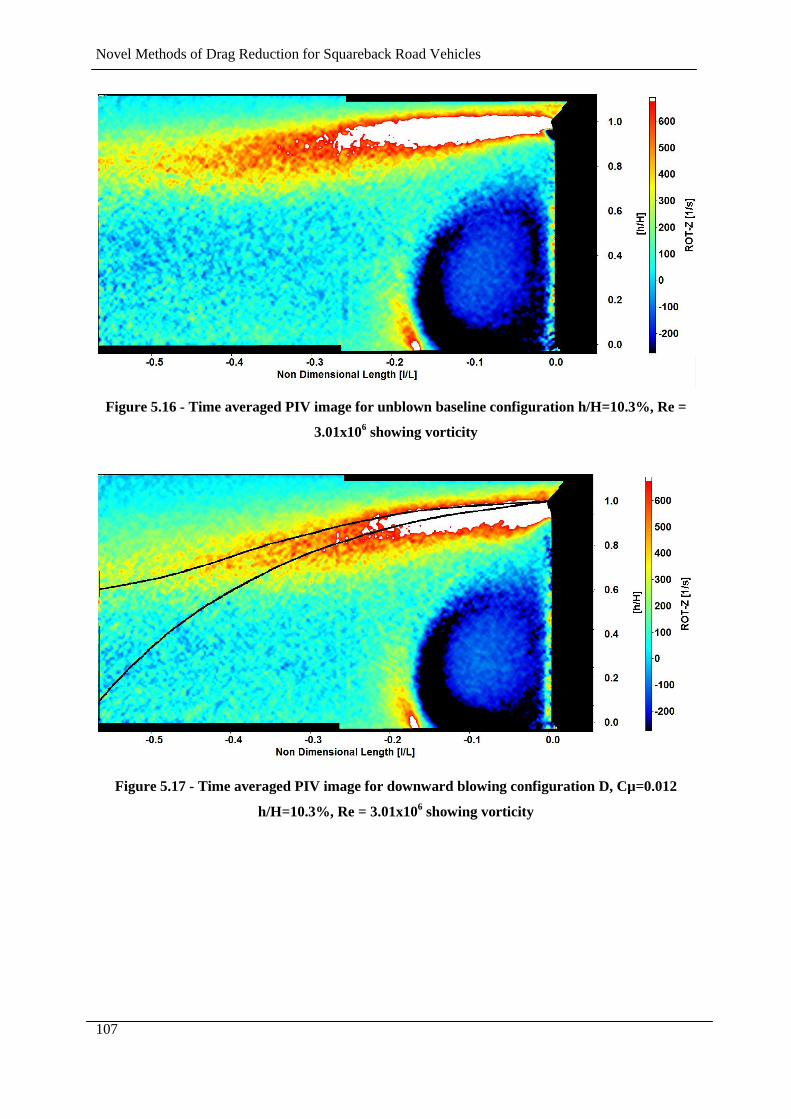
Novel Methods of Drag Reduction for Squareback Road Vehicles
107
Figure 5.16 - Time averaged PIV image for unblown baseline configuration h/H=10.3%, Re =
3.01x10⁶ showing vorticity
Figure 5.17 - Time averaged PIV image for downward blowing configuration D, Cµ=0.012
h/H=10.3%, Re = 3.01x10⁶ showing vorticity
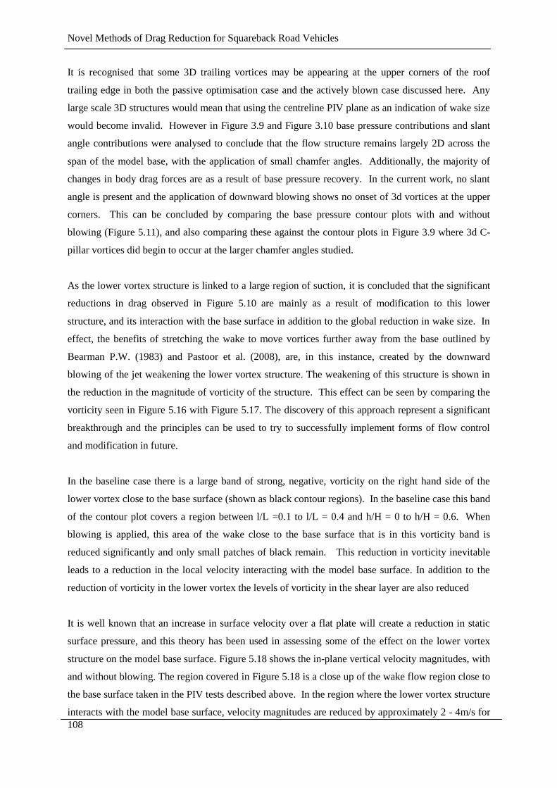
Novel Methods of Drag Reduction for Squareback Road Vehicles
108
It is recognised that some 3D trailing vortices may be appearing at the upper corners of the roof
trailing edge in both the passive optimisation case and the actively blown case discussed here. Any
large scale 3D structures would mean that using the centreline PIV plane as an indication of wake size
would become invalid. However in Figure 3.9 and Figure 3.10 base pressure contributions and slant
angle contributions were analysed to conclude that the flow structure remains largely 2D across the
span of the model base, with the application of small chamfer angles. Additionally, the majority of
changes in body drag forces are as a result of base pressure recovery. In the current work, no slant
angle is present and the application of downward blowing shows no onset of 3d vortices at the upper
corners. This can be concluded by comparing the base pressure contour plots with and without
blowing (Figure 5.11), and also comparing these against the contour plots in Figure 3.9 where 3d C-
pillar vortices did begin to occur at the larger chamfer angles studied.
As the lower vortex structure is linked to a large region of suction, it is concluded that the significant
reductions in drag observed in Figure 5.10 are mainly as a result of modification to this lower
structure, and its interaction with the base surface in addition to the global reduction in wake size. In
effect, the benefits of stretching the wake to move vortices further away from the base outlined by
Bearman P.W. (1983) and Pastoor et al. (2008), are, in this instance, created by the downward
blowing of the jet weakening the lower vortex structure. The weakening of this structure is shown in
the reduction in the magnitude of vorticity of the structure. This effect can be seen by comparing the
vorticity seen in Figure 5.16 with Figure 5.17. The discovery of this approach represent a significant
breakthrough and the principles can be used to try to successfully implement forms of flow control
and modification in future.
In the baseline case there is a large band of strong, negative, vorticity on the right hand side of the
lower vortex close to the base surface (shown as black contour regions). In the baseline case this band
of the contour plot covers a region between l/L =0.1 to l/L = 0.4 and h/H = 0 to h/H = 0.6. When
blowing is applied, this area of the wake close to the base surface that is in this vorticity band is
reduced significantly and only small patches of black remain. This reduction in vorticity inevitable
leads to a reduction in the local velocity interacting with the model base surface. In addition to the
reduction of vorticity in the lower vortex the levels of vorticity in the shear layer are also reduced
It is well known that an increase in surface velocity over a flat plate will create a reduction in static
surface pressure, and this theory has been used in assessing some of the effect on the lower vortex
structure on the model base surface. Figure 5.18 shows the in-plane vertical velocity magnitudes, with
and without blowing. The region covered in Figure 5.18 is a close up of the wake flow region close to
the base surface taken in the PIV tests described above. In the region where the lower vortex structure
interacts with the model base surface, velocity magnitudes are reduced by approximately 2 - 4m/s for
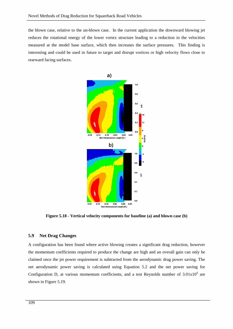
Novel Methods of Drag Reduction for Squareback Road Vehicles
109
the blown case, relative to the un-blown case. In the current application the downward blowing jet
reduces the rotational energy of the lower vortex structure leading to a reduction in the velocities
measured at the model base surface, which then increases the surface pressures. This finding is
interesting and could be used in future to target and disrupt vortices or high velocity flows close to
rearward facing surfaces.
Figure 5.18 - Vertical velocity components for baseline (a) and blown case (b)
5.9 Net Drag Changes
A configuration has been found where active blowing creates a significant drag reduction, however
the momentum coefficients required to produce the change are high and an overall gain can only be
claimed once the jet power requirement is subtracted from the aerodynamic drag power saving. The
net aerodynamic power saving is calculated using Equation 5.2 and the net power saving for
Configuration D, at various momentum coefficients, and a test Reynolds number of 3.01x10⁶ are
shown in Figure 5.19.
Novel Methods of Drag Reduction for Squareback Road Vehicles
110
Equation 5.2
Figure 5.19 - Aerodynamic Power savings available at different blowing system efficiencies
If assumptions are made that the blowing system used is 100% efficient then net aerodynamic power
savings are observed (Figure 5.19). The savings available for the wind tunnel model tested are
relatively constant up to Cµ = 0.0095, and range from 52.5W to 62.5W in this region. Above Cµ =
0.0095 the aerodynamic power savings available are reduced.
If it is possible to maintain the same balance of input power to the system vs savings in aerodynamic
drag power for a full scale vehicle rather than a ¼ scale model, the power savings could be up to 16
times greater (840W to 1kW). However, it is unknown whether the same net drag power savings
would be achievable because of the complexity of the scaling problem, which not only involves the
scaling of the physical size of the vehicle, but also the jet dimensions, and its effect on jet
performance and power consumption.
Additionally any practical system that is used to create the blowing will have losses due to efficiency,
whether from compressor efficiency or losses in pipework required to implement the system. The
effect of this efficiency term is also included in Figure 5.19, and shows a significant reduction in net
power saving as Cµ increases and ηj decreases. This illustrates that although the largest Cd reductions
are achieved with the highest Cµ available, the potential for net power savings is highest when lower
Cµ values are used. This is substantiated further when vehicle mass increases and packaging spaces
are considered; even the lower Cµ values tested require the use of heavy and physically large
Novel Methods of Drag Reduction for Squareback Road Vehicles
111
compressors and storage tanks. Vehicle mass increases will create an increase in the tractive effort
required to move the vehicle, and as such the smaller and lighter the blowing system can be used.
Currently even with the potential net aerodynamic power savings demonstrated at low Cµ values a
direct application of the technology using compressors and storage tanks is unlikely to be practical
due to the high mass flow rate requirements and consequently the need for large and heavy
equipment. However it may be possible that similar effects may be achievable using systems such as
NACA ducts to passively duct freestream flow into the wake whilst maintaining the lines and
appearance of a standard vehicle, and this is a suggested investigation for further work outside of the
current thesis. It may also be possible to reduce the duty cycle of the jet using pulsed blowing, such
that the wake flow is still modified, but the total mass flow rate requirement is reduced. Alternatively
a pulsed jet may induce some of the effects that have been described when using Synthetic Jets and
also help to recover pressure in the wake by using specific excitation frequencies.
Application of SJ actuators to the Windsor model has been avoided because of the lack of available
momentum coefficient and the number of performance variables that raised doubts about their
successful application. However, a pressurised cavity with controllable valves that can create a
consistent mass outlet flux whilst also being able to control actuation frequency may lead to further
understanding of how pulsed jet excitations may affect base pressures.
5.10 Discussion
The influence of steady blowing applied at a variety of angles on the roof trailing edge of a simplified
¼ scale square-back style vehicle has been investigated. Increases in measured drag coefficient were
observed for all configurations tested except for the ’45 degrees down’ configuration, where large
improvements in drag are possible.
The changes in drag coefficient were corrected for blockage effects and the influence of jet thrust has
been subtracted. Where significant drag reductions were observed an effort has been made to
understand the mechanisms which cause this change. For these configurations the majority of changes
in drag forces are as a result of base pressure modification which has been supported using an area
weighted base pressure coefficient calculation.
In the cases tested at Re = 3.01x10⁶ the reduction in drag observed when blowing was applied at a 45˚
downwards angle has been attributed to a reduction in wake size via a deflection of the upper shear
layer downwards and reduction in the levels of vorticity found in the wake. This reduction in

Novel Methods of Drag Reduction for Squareback Road Vehicles
112
vorticity in the lower vortex structure leads to a reduction in the local surface velocities on the model
base. The vorticity of the lower wake structure is reduced by the jet flow opposing the direction of
rotation of the large lower vortex.
Although the highest reductions in Cd are achieved at the highest Cµ configurations tested, an analysis
of the net change in aerodynamic power has revealed that a system would be most efficient using low
Cµ configurations.
Although the current work shows promise for the use of active blowing the current mass flow rates
required would be prohibitive when trying to directly implement the techniques to a production road
vehicle. The use of passive ducting of freestream flow may allow the technique to be exploited whilst
still maintaining global vehicle shapes and packaging requirements. The next stage of investigations
should look for lower energy demand means of creating the saving found in this chapter.
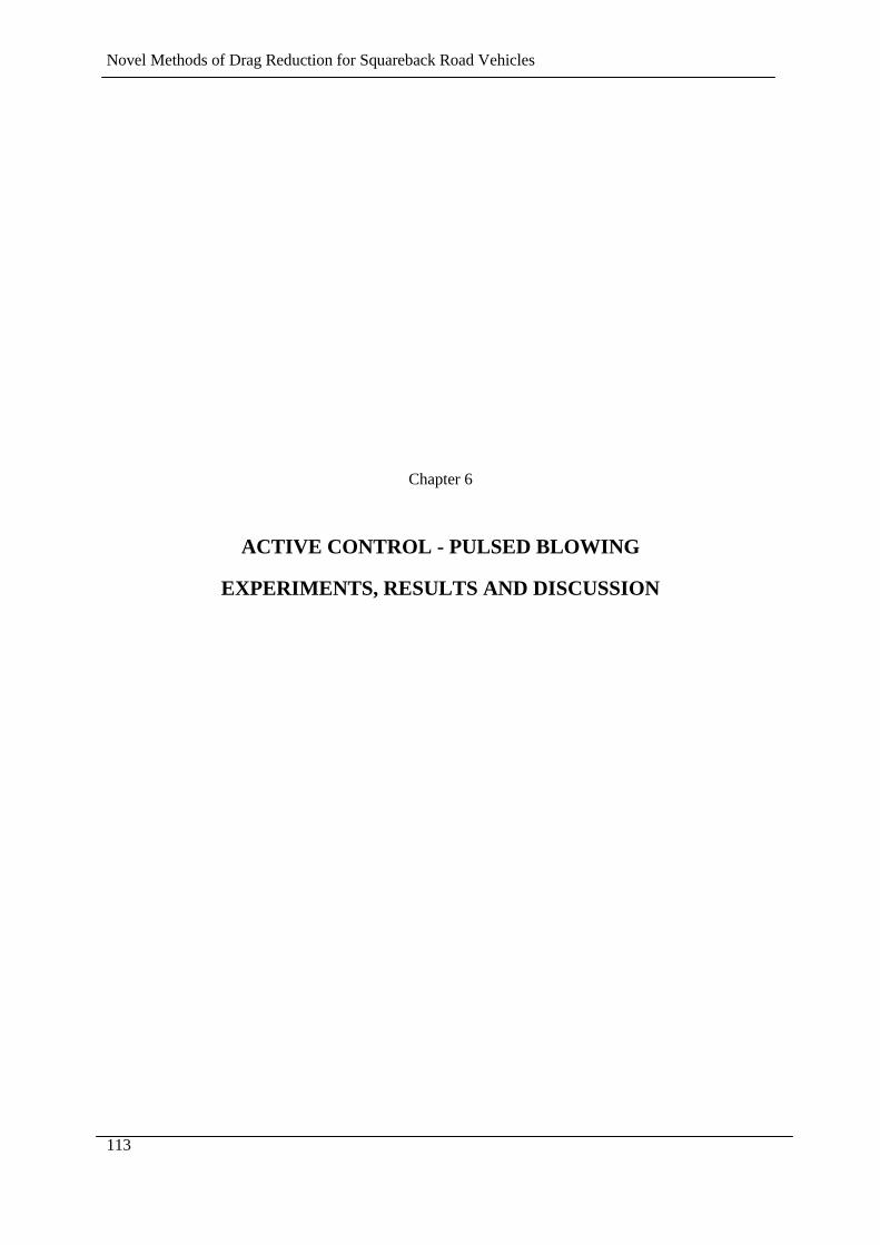
Novel Methods of Drag Reduction for Squareback Road Vehicles
113
Chapter 6
ACTIVE CONTROL - PULSED BLOWING
EXPERIMENTS, RESULTS AND DISCUSSION
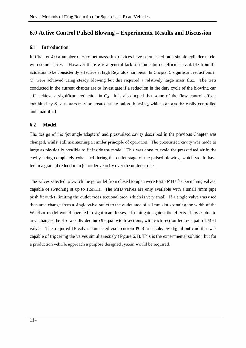
Novel Methods of Drag Reduction for Squareback Road Vehicles
114
6.0 Active Control Pulsed Blowing – Experiments, Results and Discussion
6.1 Introduction
In Chapter 4.0 a number of zero net mass flux devices have been tested on a simple cylinder model
with some success. However there was a general lack of momentum coefficient available from the
actuators to be consistently effective at high Reynolds numbers. In Chapter 5 significant reductions in
Cd were achieved using steady blowing but this required a relatively large mass flux. The tests
conducted in the current chapter are to investigate if a reduction in the duty cycle of the blowing can
still achieve a significant reduction in Cd. It is also hoped that some of the flow control effects
exhibited by SJ actuators may be created using pulsed blowing, which can also be easily controlled
and quantified.
6.2 Model
The design of the ‘jet angle adapters’ and pressurised cavity described in the previous Chapter was
changed, whilst still maintaining a similar principle of operation. The pressurised cavity was made as
large as physically possible to fit inside the model. This was done to avoid the pressurised air in the
cavity being completely exhausted during the outlet stage of the pulsed blowing, which would have
led to a gradual reduction in jet outlet velocity over the outlet stroke.
The valves selected to switch the jet outlet from closed to open were Festo MHJ fast switching valves,
capable of switching at up to 1.5KHz. The MHJ valves are only available with a small 4mm pipe
push fit outlet, limiting the outlet cross sectional area, which is very small. If a single valve was used
then area change from a single valve outlet to the outlet area of a 1mm slot spanning the width of the
Windsor model would have led to significant losses. To mitigate against the effects of losses due to
area changes the slot was divided into 9 equal width sections, with each section fed by a pair of MHJ
valves. This required 18 valves connected via a custom PCB to a Labview digital out card that was
capable of triggering the valves simultaneously (Figure 6.1). This is the experimental solution but for
a production vehicle approach a purpose designed system would be required.
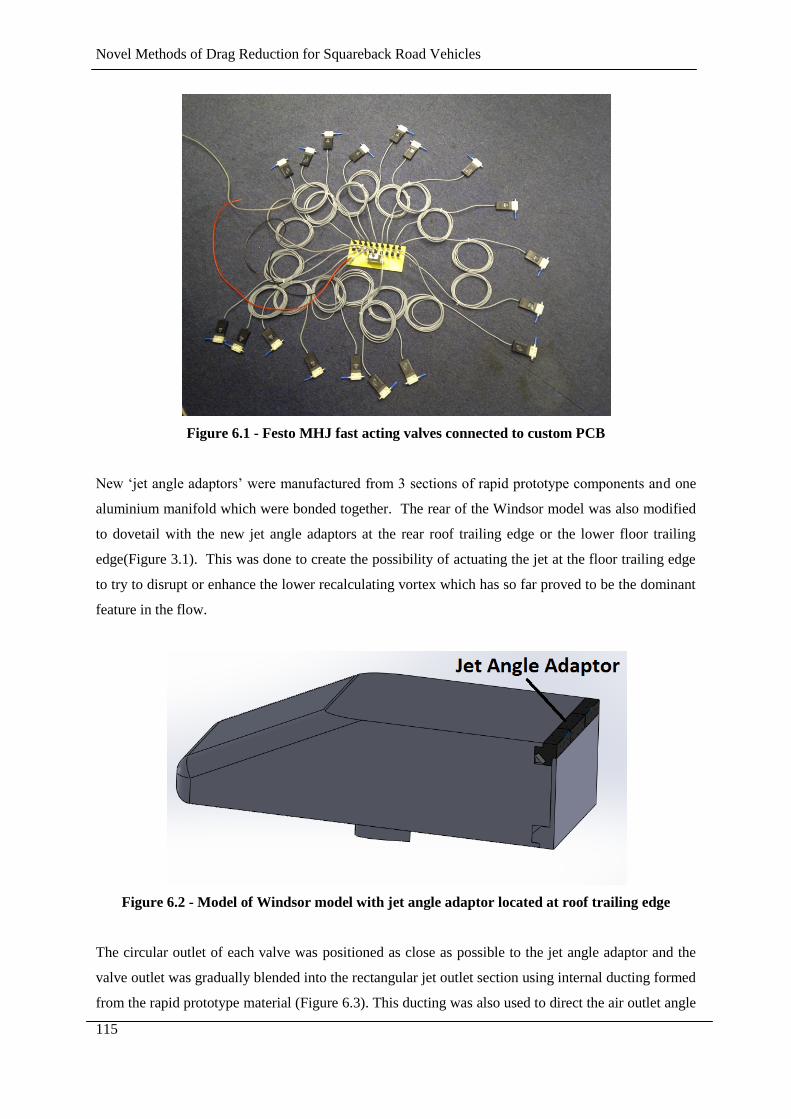
Novel Methods of Drag Reduction for Squareback Road Vehicles
115
Figure 6.1 - Festo MHJ fast acting valves connected to custom PCB
New ‘jet angle adaptors’ were manufactured from 3 sections of rapid prototype components and one
aluminium manifold which were bonded together. The rear of the Windsor model was also modified
to dovetail with the new jet angle adaptors at the rear roof trailing edge or the lower floor trailing
edge(Figure 3.1). This was done to create the possibility of actuating the jet at the floor trailing edge
to try to disrupt or enhance the lower recalculating vortex which has so far proved to be the dominant
feature in the flow.
Figure 6.2 - Model of Windsor model with jet angle adaptor located at roof trailing edge
The circular outlet of each valve was positioned as close as possible to the jet angle adaptor and the
valve outlet was gradually blended into the rectangular jet outlet section using internal ducting formed
from the rapid prototype material (Figure 6.3). This ducting was also used to direct the air outlet angle
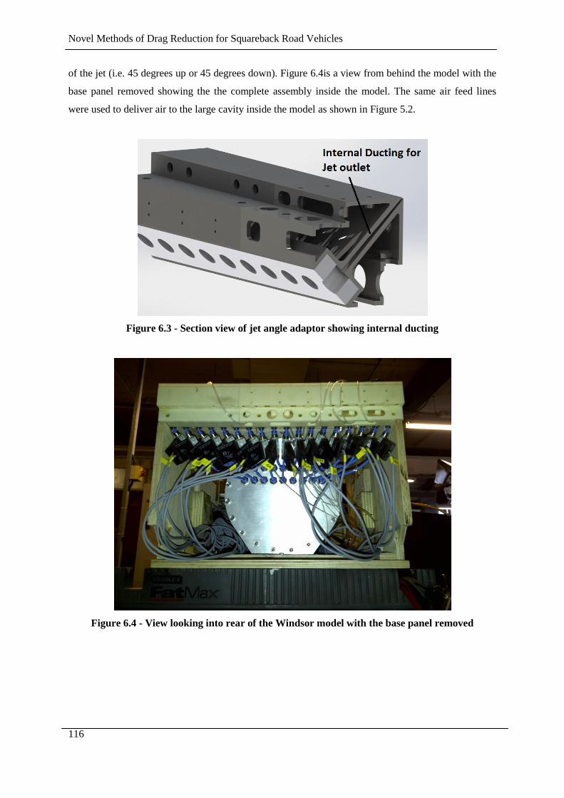
Novel Methods of Drag Reduction for Squareback Road Vehicles
116
of the jet (i.e. 45 degrees up or 45 degrees down). Figure 6.4is a view from behind the model with the
base panel removed showing the the complete assembly inside the model. The same air feed lines
were used to deliver air to the large cavity inside the model as shown in Figure 5.2.
Figure 6.3 - Section view of jet angle adaptor showing internal ducting
Figure 6.4 - View looking into rear of the Windsor model with the base panel removed
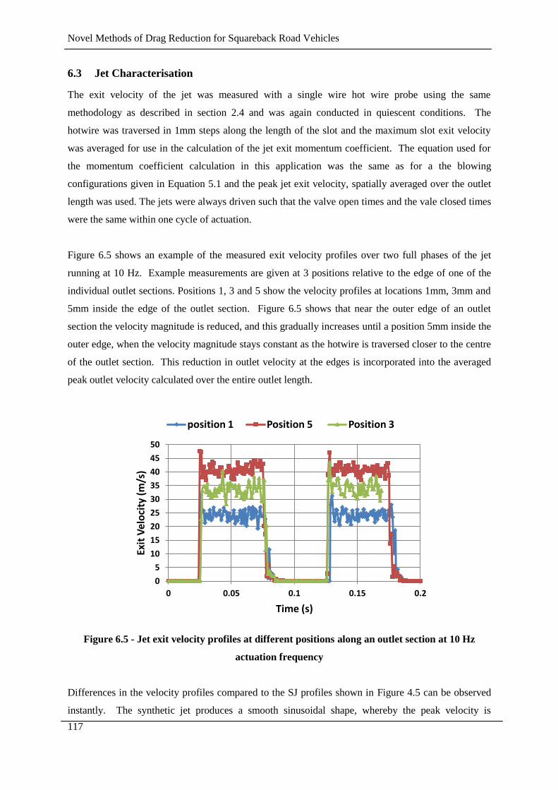
Novel Methods of Drag Reduction for Squareback Road Vehicles
117
6.3 Jet Characterisation
The exit velocity of the jet was measured with a single wire hot wire probe using the same
methodology as described in section 2.4 and was again conducted in quiescent conditions. The
hotwire was traversed in 1mm steps along the length of the slot and the maximum slot exit velocity
was averaged for use in the calculation of the jet exit momentum coefficient. The equation used for
the momentum coefficient calculation in this application was the same as for a the blowing
configurations given in Equation 5.1 and the peak jet exit velocity, spatially averaged over the outlet
length was used. The jets were always driven such that the valve open times and the vale closed times
were the same within one cycle of actuation.
Figure 6.5 shows an example of the measured exit velocity profiles over two full phases of the jet
running at 10 Hz. Example measurements are given at 3 positions relative to the edge of one of the
individual outlet sections. Positions 1, 3 and 5 show the velocity profiles at locations 1mm, 3mm and
5mm inside the edge of the outlet section. Figure 6.5 shows that near the outer edge of an outlet
section the velocity magnitude is reduced, and this gradually increases until a position 5mm inside the
outer edge, when the velocity magnitude stays constant as the hotwire is traversed closer to the centre
of the outlet section. This reduction in outlet velocity at the edges is incorporated into the averaged
peak outlet velocity calculated over the entire outlet length.
Figure 6.5 - Jet exit velocity profiles at different positions along an outlet section at 10 Hz
actuation frequency
Differences in the velocity profiles compared to the SJ profiles shown in Figure 4.5 can be observed
instantly. The synthetic jet produces a smooth sinusoidal shape, whereby the peak velocity is
0
5
10
15
20
25
30
35
40
45
50
0 0.05 0.1 0.15 0.2
Exit
Vel
oci
ty (
m/s
)
Time (s)
position 1 Position 5 Position 3

Novel Methods of Drag Reduction for Squareback Road Vehicles
118
achieved gradually and then the inward stroke pulls the outlet speeds back down to a minimum. For
the pulsed jet configuration the outlet stroke is in the form of a square wave with a very fast
development of the peak velocity as the valve opens, and a sharp reduction to 0m/s as the valve
closes.
During the ‘valve closed’ section of the cycle the measured velocity is 0m/s indicating that the valves
form a good seal and no leakage occurs. Using position 5 as an example; as the valve opens a large
pulse of velocity is measured up to ~47m/s. This pulse quickly settles to an almost constant value of
~41 m/s. For lower frequencies such as the 1Hz signal shown in Figure 6.6 a slight decay in the exit
velocity can be observed over the ‘valve open’ section of the cycle. This effect has been minimised
by using as large a pressurised cavity as physically possible but some effect is still present. Even
though this decay is present the mean outlet velocity throughout the outlet phase of the cycle is 41m/s.
The fact that the average outlet velocity at 1Hz is the same as at 10Hz demonstrates that it is possible
to achieve consistent momentum coefficients whilst modifying the actuation frequency of the jets.
This was controlled via the measurement and control of the pressure in the cavity that supplies the jet
outlets.
Figure 6.6 - Jet exit velocity profile at position 5 for an actuation frequency of 1Hz
0
5
10
15
20
25
30
35
40
45
50
55
60
0 0.2 0.4 0.6 0.8 1 1.2 1.4 1.6 1.8
Exit
Vel
oci
tyt
(m/s
)
Time (s)
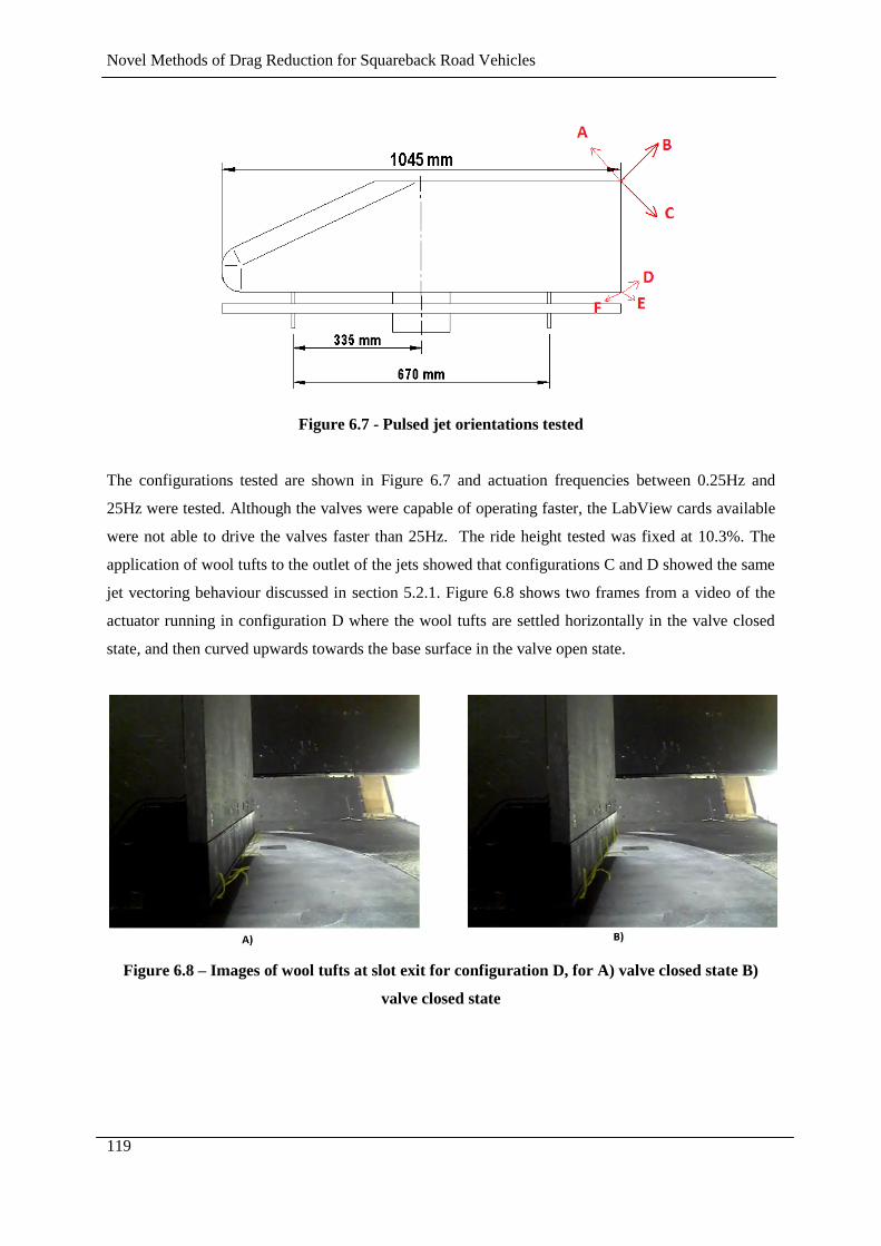
Novel Methods of Drag Reduction for Squareback Road Vehicles
119
Figure 6.7 - Pulsed jet orientations tested
The configurations tested are shown in Figure 6.7 and actuation frequencies between 0.25Hz and
25Hz were tested. Although the valves were capable of operating faster, the LabView cards available
were not able to drive the valves faster than 25Hz. The ride height tested was fixed at 10.3%. The
application of wool tufts to the outlet of the jets showed that configurations C and D showed the same
jet vectoring behaviour discussed in section 5.2.1. Figure 6.8 shows two frames from a video of the
actuator running in configuration D where the wool tufts are settled horizontally in the valve closed
state, and then curved upwards towards the base surface in the valve open state.
Figure 6.8 – Images of wool tufts at slot exit for configuration D, for A) valve closed state B)
valve closed state
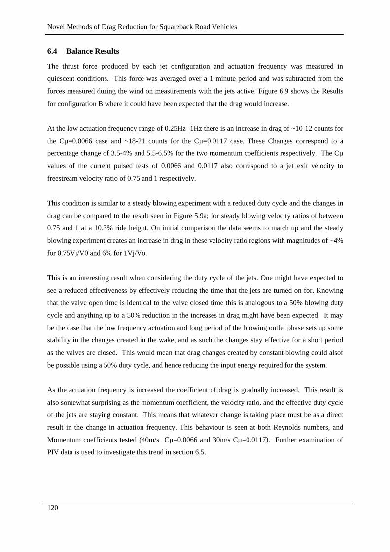
Novel Methods of Drag Reduction for Squareback Road Vehicles
120
6.4 Balance Results
The thrust force produced by each jet configuration and actuation frequency was measured in
quiescent conditions. This force was averaged over a 1 minute period and was subtracted from the
forces measured during the wind on measurements with the jets active. Figure 6.9 shows the Results
for configuration B where it could have been expected that the drag would increase.
At the low actuation frequency range of 0.25Hz -1Hz there is an increase in drag of ~10-12 counts for
the Cµ=0.0066 case and ~18-21 counts for the Cµ=0.0117 case. These Changes correspond to a
percentage change of 3.5-4% and 5.5-6.5% for the two momentum coefficients respectively. The Cµ
values of the current pulsed tests of 0.0066 and 0.0117 also correspond to a jet exit velocity to
freestream velocity ratio of 0.75 and 1 respectively.
This condition is similar to a steady blowing experiment with a reduced duty cycle and the changes in
drag can be compared to the result seen in Figure 5.9a; for steady blowing velocity ratios of between
0.75 and 1 at a 10.3% ride height. On initial comparison the data seems to match up and the steady
blowing experiment creates an increase in drag in these velocity ratio regions with magnitudes of ~4%
for 0.75Vj/V0 and 6% for 1Vj/Vo.
This is an interesting result when considering the duty cycle of the jets. One might have expected to
see a reduced effectiveness by effectively reducing the time that the jets are turned on for. Knowing
that the valve open time is identical to the valve closed time this is analogous to a 50% blowing duty
cycle and anything up to a 50% reduction in the increases in drag might have been expected. It may
be the case that the low frequency actuation and long period of the blowing outlet phase sets up some
stability in the changes created in the wake, and as such the changes stay effective for a short period
as the valves are closed. This would mean that drag changes created by constant blowing could alsof
be possible using a 50% duty cycle, and hence reducing the input energy required for the system.
As the actuation frequency is increased the coefficient of drag is gradually increased. This result is
also somewhat surprising as the momentum coefficient, the velocity ratio, and the effective duty cycle
of the jets are staying constant. This means that whatever change is taking place must be as a direct
result in the change in actuation frequency. This behaviour is seen at both Reynolds numbers, and
Momentum coefficients tested (40m/s Cµ=0.0066 and 30m/s Cµ=0.0117). Further examination of
PIV data is used to investigate this trend in section 6.5.
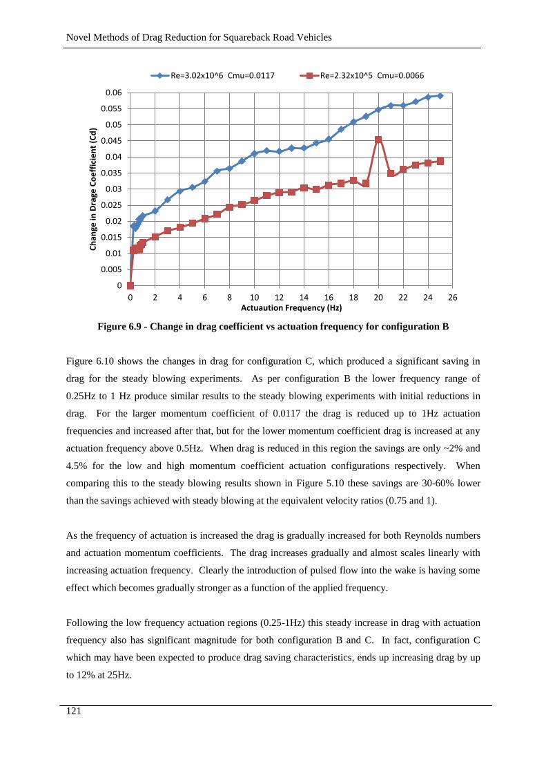
Novel Methods of Drag Reduction for Squareback Road Vehicles
121
Figure 6.9 - Change in drag coefficient vs actuation frequency for configuration B
Figure 6.10 shows the changes in drag for configuration C, which produced a significant saving in
drag for the steady blowing experiments. As per configuration B the lower frequency range of
0.25Hz to 1 Hz produce similar results to the steady blowing experiments with initial reductions in
drag. For the larger momentum coefficient of 0.0117 the drag is reduced up to 1Hz actuation
frequencies and increased after that, but for the lower momentum coefficient drag is increased at any
actuation frequency above 0.5Hz. When drag is reduced in this region the savings are only ~2% and
4.5% for the low and high momentum coefficient actuation configurations respectively. When
comparing this to the steady blowing results shown in Figure 5.10 these savings are 30-60% lower
than the savings achieved with steady blowing at the equivalent velocity ratios (0.75 and 1).
As the frequency of actuation is increased the drag is gradually increased for both Reynolds numbers
and actuation momentum coefficients. The drag increases gradually and almost scales linearly with
increasing actuation frequency. Clearly the introduction of pulsed flow into the wake is having some
effect which becomes gradually stronger as a function of the applied frequency.
Following the low frequency actuation regions (0.25-1Hz) this steady increase in drag with actuation
frequency also has significant magnitude for both configuration B and C. In fact, configuration C
which may have been expected to produce drag saving characteristics, ends up increasing drag by up
to 12% at 25Hz.
0
0.005
0.01
0.015
0.02
0.025
0.03
0.035
0.04
0.045
0.05
0.055
0.06
0 2 4 6 8 10 12 14 16 18 20 22 24 26
Ch
ange
in D
rage
Co
eff
icie
nt
(Cd
)
Actuaution Frequency (Hz)
Re=3.02x10^6 Cmu=0.0117 Re=2.32x10^5 Cmu=0.0066

Novel Methods of Drag Reduction for Squareback Road Vehicles
122
Figure 6.10 - Change in drag coefficient vs actuation frequency for configuration C
Configurations D,E and F were incorporated to investigate if the strength of the lower vortex structure
could be disrupted by applying pulsed blowing at the floor trailing edge. Figure 6.11 shows the
balance results for these configurations and shows configurations E and F only ever increase the total
amount of drag. For both E and F the initial application of pulsed blowing creates a sharp increase in
drag coefficient with respect to the baseline configuration, but Configuration F has a much larger
effect than configuration E. The significant effects seen in configuration F are a result of the
significant disruption applied to the underbody flow by the forward facing jets, where as the effects
created from jet configuration E are somewhat more subtle.
As frequency is increased whilst maintaining a fixed momentum coefficient, drag changes are
gradually increased for both configurations, but again the forward facing jets of configuration F create
greater gradient of change than configuration E.
-0.01
-0.005
0
0.005
0.01
0.015
0.02
0.025
0.03
0.035
0.04
0.045
0.05
0 2 4 6 8 10 12 14 16 18 20 22 24 26
Ch
ange
in D
rag
Co
eff
icie
nt
(Cd
)
Actuation Frequency (Hz)
RE = 2.32x10^5 Cmu =0. 0117 Re = 3.02x10^6 Cmu =0.0066
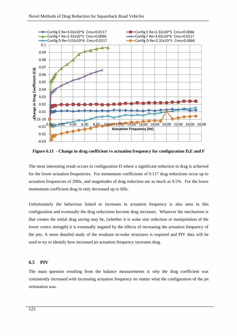
Novel Methods of Drag Reduction for Squareback Road Vehicles
123
Figure 6.11 - Change in drag coefficient vs actuation frequency for configuration D,E and F
The most interesting result occurs in configuration D where a significant reduction in drag is achieved
for the lower actuation frequencies. For momentum coefficients of 0.117 drag reductions occur up to
actuation frequencies of 20Hz, and magnitudes of drag reduction are as much as 9.5%. For the lower
momentum coefficient drag in only decreased up to 6Hz.
Unfortunately the behaviour linked to increases in actuation frequency is also seen in this
configuration and eventually the drag reductions become drag increases. Whatever the mechanism is
that creates the initial drag saving may be, (whether it is wake size reduction or manipulation of the
lower vortex strength) it is eventually negated by the effects of increasing the actuation frequency of
the jets. A more detailed study of the resultant in-wake structures is required and PIV data will be
used to try to identify how increased jet actuation frequency increases drag.
6.5 PIV
The main question resulting from the balance measurements is why the drag coefficient was
consistently increased with increasing actuation frequency no matter what the configuration of the jet
orientation was.
-0.03
-0.02
-0.01
3.1E-16
0.01
0.02
0.03
0.04
0.05
0.06
0.07
0.08
0.09
0.1
0.00 2.00 4.00 6.00 8.00 10.00 12.00 14.00 16.00 18.00 20.00 22.00 24.00 26.00
Ch
ange
in D
rag
Co
eff
icie
nt
(Cd
)
Actuation Frequency (Hz)
Config E Re=3.02x10^6 Cmu=0.0117 Config E Re=2.32x10^5 Cmu=0.0066 Config F Re=2.32x10^5 Cmu=0.0066 Config F Re=3.02x10^6 Cmu=0.0117 Config D Re=3.02x10^6 Cmu=0.0117 Config D Re=2.32x10^5 Cmu=0.0066

Novel Methods of Drag Reduction for Squareback Road Vehicles
124
6.5.1 Configuration B
From the previous chapters it has been identified that total body drag can be modified by modifying
the base pressure distribution. The main area to be targeted is the lower half of the base where surface
pressure distributions can be modified by changing the position and strength of the lower vortex. In
addition to targeting this vortex overall wake size will influence the global base pressures.
PIV data for configuration B, for steady blowing, 10Hz actuation and 25Hz actuation is shown in
Figure 6.12. The data shows vorticity values as a contour plot with velocity vectors in the foreground.
With steady blowing it is seen that the wake is large with the shear layer being deflected up and out of
the top of the FoV (as shown in section 5.8) As the actuation is changed from steady blowing to a
pulsed actuation at 10 Hz the total wake size is actually reduced, with the upper shear layer seemingly
being turned downwards by the cyclic actuation. The wake size continues to be reduced slightly as
the actuation frequency is increased from 10Hz to 25Hz.
In addition to the wake size being reduced when the blowing is pulsed the total size of the lower
vortex is also reduced (which is the opposite of what one might expect from the previous blowing
investigations) as the drag increases with increasing actuation frequency.
At 10Hz the lower vortex interacts with the base up to h/H~0.7 and at 25Hz the lower vortex only
reaches up to h/H~0.65. However as the size of the wake is reduced the levels of vorticity in the
lower vortex increase; at 10Hz there is clockwise vorticity near the base from ~200-250s-1
but at 25Hz
the clockwise vorticity near the base surface is increased to 250-300s-1
. In addition to an increase in
levels of clockwise vorticity in the mid-lower half of the wake, the anticlockwise vorticity in the
upper half of the wake is also increased by the application of pulsed blowing. At an actuation
frequency of 25Hz, levels of clockwise vorticity close to the base surface above h/H=0.65 are of a
magnitude between 100-300s-1
.
From the data presented in Figure 6.12 it appears that as actuation frequency is increased the strength
of the vortical structures close to the base surface is increased. As the strength of these vortices is
increased the base surface velocities will be increased and base surface pressures will be decreased as
a result. In order to try to quantify the increase in vortex strength the vorticity levels close to the base
are analysed further.
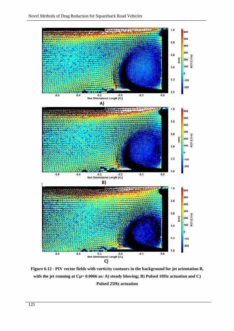
Novel Methods of Drag Reduction for Squareback Road Vehicles
125
Figure 6.12 - PIV vector fields with vorticity contours in the background for jet orientation B,
with the jet running at Cµ= 0.0066 as: A) steady blowing; B) Pulsed 10Hz actuation and C)
Pulsed 25Hz actuation
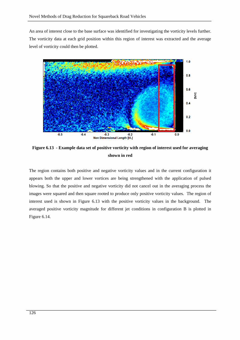
Novel Methods of Drag Reduction for Squareback Road Vehicles
126
An area of interest close to the base surface was identified for investigating the vorticity levels further.
The vorticity data at each grid position within this region of interest was extracted and the average
level of vorticity could then be plotted.
Figure 6.13 - Example data set of positive vorticity with region of interest used for averaging
shown in red
The region contains both positive and negative vorticity values and in the current configuration it
appears both the upper and lower vortices are being strengthened with the application of pulsed
blowing. So that the positive and negative vorticity did not cancel out in the averaging process the
images were squared and then square rooted to produce only positive vorticity values. The region of
interest used is shown in Figure 6.13 with the positive vorticity values in the background. The
averaged positive vorticity magnitude for different jet conditions in configuration B is plotted in
Figure 6.14.
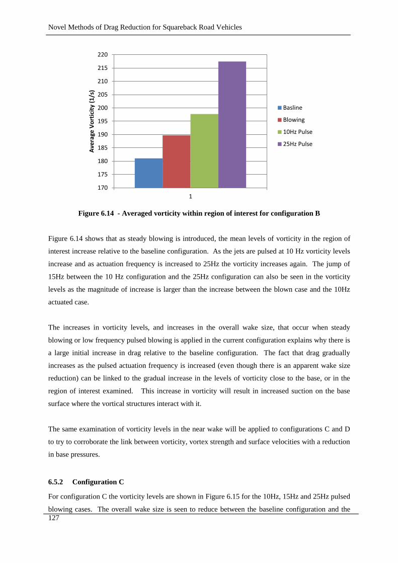
Novel Methods of Drag Reduction for Squareback Road Vehicles
127
Figure 6.14 - Averaged vorticity within region of interest for configuration B
Figure 6.14 shows that as steady blowing is introduced, the mean levels of vorticity in the region of
interest increase relative to the baseline configuration. As the jets are pulsed at 10 Hz vorticity levels
increase and as actuation frequency is increased to 25Hz the vorticity increases again. The jump of
15Hz between the 10 Hz configuration and the 25Hz configuration can also be seen in the vorticity
levels as the magnitude of increase is larger than the increase between the blown case and the 10Hz
actuated case.
The increases in vorticity levels, and increases in the overall wake size, that occur when steady
blowing or low frequency pulsed blowing is applied in the current configuration explains why there is
a large initial increase in drag relative to the baseline configuration. The fact that drag gradually
increases as the pulsed actuation frequency is increased (even though there is an apparent wake size
reduction) can be linked to the gradual increase in the levels of vorticity close to the base, or in the
region of interest examined. This increase in vorticity will result in increased suction on the base
surface where the vortical structures interact with it.
The same examination of vorticity levels in the near wake will be applied to configurations C and D
to try to corroborate the link between vorticity, vortex strength and surface velocities with a reduction
in base pressures.
6.5.2 Configuration C
For configuration C the vorticity levels are shown in Figure 6.15 for the 10Hz, 15Hz and 25Hz pulsed
blowing cases. The overall wake size is seen to reduce between the baseline configuration and the
170
175
180
185
190
195
200
205
210
215
220
1
Ave
rage
Vo
rtic
ity
(1/s
)
Basline
Blowing
10Hz Pulse
25Hz Pulse

Novel Methods of Drag Reduction for Squareback Road Vehicles
128
10Hz pulsed jet results. The wake size also continues to reduce even between the 10Hz and 25Hz
cases, which is seen as the shear layer being deflected downwards. This wake size reduction is
occurring as the total drag force is increasing (Figure 6.10).
The overall size of the lower vortex structure remains relatively constant as actuation frequency is
increased with the top of the structures located ~h/H = 0.65 (Figure 6.15). The levels of clockwise
vorticity within the lower vortex gradually increase with frequency shown by the appearance of more
black contour plot regions. In addition to the increases in vorticity in the lower wake the levels of anti-
clockwise vorticity in the upper wake are increase, shown as more yellow regions of the contour plot
close to the upper base surface.
The averaged magnitudes of vorticity within the region of interest shown in Figure 6.13 are plotted in
Figure 6.16 for configuration C. This plot also shows a link between the levels of vorticity and the
increasing drag forces associated with increased actuation frequency (Figure 6.10). The level of
vorticity for the low frequency actuation at 1Hz is slightly reduced relative to the baseline case but the
magnitudes of change are not significant. As frequency is increased so too do the levels of vorticity
by up to 40s-1
which reinforces theory that there is a direct link between the increasing drag forces
with the increased vorticity observed as actuation frequency increases.

Novel Methods of Drag Reduction for Squareback Road Vehicles
129
Figure 6.15 - PIV vector fields with vorticity contours in the background for jet orientation C,
with the jet running at Cµ= 0.0066 as: A) Pulsed 10 Hz actuation; B) Pulsed 15Hz actuation
and C) Pulsed 25Hz actuation

Novel Methods of Drag Reduction for Squareback Road Vehicles
130
Figure 6.16 - Averaged vorticity within region of interest for configuration C
6.5.3 Configuration D
Configuration D showed significant reductions in drag for the lower actuation frequencies with the
characteristic increase in drag at higher frequencies. On examination of the PIV data (Figure 6.17) for
the lower frequencies it can be seen that the wake size does not change significantly relative to the
baseline, however the vorticity in the lower vortex is reduced. It is only at the higher frequency of
25Hz where the upper shear layer is seen to be deflected upwards and increases the overall wake size.
In addition to the increase in wake size a significant amount of vorticity is seen in the lower vortex at
25Hz.
The rotational energy in the lower vortex is reduced at lower actuation frequencies by virtue of the
direction at which the jet exits. The actual outlet direction of the jet is ~10 degrees off vertical (see
Figure 5.6) which would oppose the downward flow along the base surface created by the lower
vortex. As actuation frequencies are increased the jet becomes less able to oppose the downward flow
direction created by the lower vortex and the effects created by pulsing the flow dominate, leading to
an increase in the lower vortex strength.
170
180
190
200
210
220
1
Ave
rage
Vo
rtic
ity
(1/s
)
Baseline
1Hz Pulsed
15Hz Pulsed
20Hz Pulsed
25Hz Pulsed
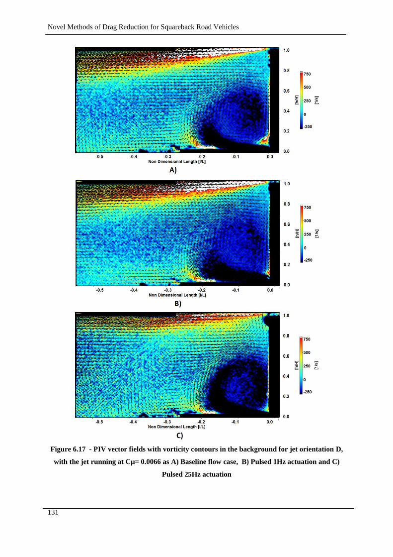
Novel Methods of Drag Reduction for Squareback Road Vehicles
131
Figure 6.17 - PIV vector fields with vorticity contours in the background for jet orientation D,
with the jet running at Cµ= 0.0066 as A) Baseline flow case, B) Pulsed 1Hz actuation and C)
Pulsed 25Hz actuation
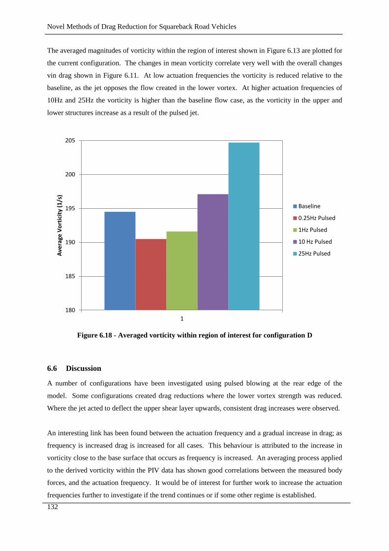
Novel Methods of Drag Reduction for Squareback Road Vehicles
132
The averaged magnitudes of vorticity within the region of interest shown in Figure 6.13 are plotted for
the current configuration. The changes in mean vorticity correlate very well with the overall changes
vin drag shown in Figure 6.11. At low actuation frequencies the vorticity is reduced relative to the
baseline, as the jet opposes the flow created in the lower vortex. At higher actuation frequencies of
10Hz and 25Hz the vorticity is higher than the baseline flow case, as the vorticity in the upper and
lower structures increase as a result of the pulsed jet.
Figure 6.18 - Averaged vorticity within region of interest for configuration D
6.6 Discussion
A number of configurations have been investigated using pulsed blowing at the rear edge of the
model. Some configurations created drag reductions where the lower vortex strength was reduced.
Where the jet acted to deflect the upper shear layer upwards, consistent drag increases were observed.
An interesting link has been found between the actuation frequency and a gradual increase in drag; as
frequency is increased drag is increased for all cases. This behaviour is attributed to the increase in
vorticity close to the base surface that occurs as frequency is increased. An averaging process applied
to the derived vorticity within the PIV data has shown good correlations between the measured body
forces, and the actuation frequency. It would be of interest for further work to increase the actuation
frequencies further to investigate if the trend continues or if some other regime is established.
180
185
190
195
200
205
1
Ave
rage
Vo
rtic
ity
(1/s
)
Baseline
0.25Hz Pulsed
1Hz Pulsed
10 Hz Pulsed
25Hz Pulsed

Novel Methods of Drag Reduction for Squareback Road Vehicles
133
The required mass flow has been reduced by pulsing the jets, however in all cases where a drag
reduction occurred, the savings were also reduced. The switching of the valves requires an energy
input and as such the pulsing of the jets does not offer any improvement over the standard blowing
system.
The additional investigations carried out at the lower edge of the model have again shown that drag
can be reduced if the energy within the lower vortex structure is manipulated. The previous
investigations with active blowing and pulsed blowing create questions regarding if this effect can be
created passively. Potentially this could be achieved using ducted freestream flow, or alternatively
the lower vortex strength could be disrupted with some form of discrete shape change on the base
surface.
Novel Methods of Drag Reduction for Squareback Road Vehicles
134
Chapter 7
PASSIVE CONTROL OF IN WAKE STRUCTURES
EXPERIMENTS, RESULTS AND DISCUSSION
Novel Methods of Drag Reduction for Squareback Road Vehicles
135
7.0 Passive Control of In Wake Structures – Experiments, Results and
Discussion
7.1 Introduction
In the experiments conducted in the previous Chapters it has been shown that the manipulation of the
vehicle wake size alone is not the only factor that will influence base pressures. The large lower
vortex structure in the near wake of the model is consistently linked to a region of low pressure on the
base. In the previous chapters it has been argued that reducing the vorticity of this structure can cause
an increase in base pressure, and in fact an increase in vorticity introduced by pulsed jets will actually
increase the drag force on the body. It has also been argued that applying constant blowing from the
upper rear roof trailing edge to reduce the vorticy creates a reduction in the downward flow velocity
moving over the base surface, which in turn creates a drag reduction.
It is clear the way in which the lower vortex structure interacts with the base surface plays a large role
in creation of the level of negative pressure on the base surface. The same dependence of base surface
pressures on vortex structure interaction has been observed by other authors (Bearman, 1965) (Pastoor
et al., 2008) and the manipulation of this interaction has been used to change vehicle drag forces. In
the current chapter small passive features are added to the lower half of the base surface to try to
manipulate the way in which the lower vortex structure interacts with it. The intention is to reduce the
downward flow velocity over the base surface and reduce vorticity, causing an increase in base
pressures. The fact that these passive modifications do not require an energy input means that any
saving found here will all directly contribute to a reduction in the vehicle power requirements.
In addition to testing at model scale there was a short opportunity to test the theories outlined below at
full scale on a production vehicle to investigate if the effects observed scale efficiently.
7.2 Experimental Configurations
7.2.1 Model Scale
The standard configuration of the base surface on the Windsor model is flat and perpendicular to the
onset flow direction. As a means of testing the theory that disrupting the lower vortex structure can
induce a drag saving some simple passive modifications to the Windsor model were designed. For the
different configurations the model was fitted with small 1mm thick, 8mm deep ‘slats’ on the lower
half of its base surface, as shown in detail A of Figure 7.1. The first slat added was positioned 35mm
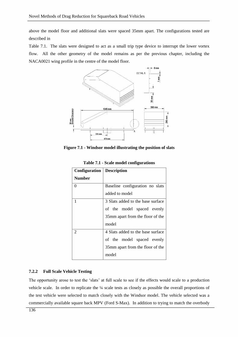
Novel Methods of Drag Reduction for Squareback Road Vehicles
136
above the model floor and additional slats were spaced 35mm apart. The configurations tested are
described in
Table 7.1. The slats were designed to act as a small trip type device to interrupt the lower vortex
flow. All the other geometry of the model remains as per the previous chapter, including the
NACA0021 wing profile in the centre of the model floor.
Figure 7.1 - Windsor model illustrating the position of slats
Table 7.1 - Scale model configurations
Configuration
Number
Description
0 Baseline configuration no slats
added to model
1 3 Slats added to the base surface
of the model spaced evenly
35mm apart from the floor of the
model
2 4 Slats added to the base surface
of the model spaced evenly
35mm apart from the floor of the
model
7.2.2 Full Scale Vehicle Testing
The opportunity arose to test the ‘slats’ at full scale to see if the effects would scale to a production
vehicle scale. In order to replicate the ¼ scale tests as closely as possible the overall proportions of
the test vehicle were selected to match closely with the Windsor model. The vehicle selected was a
commercially available square back MPV (Ford S-Max). In addition to trying to match the overbody
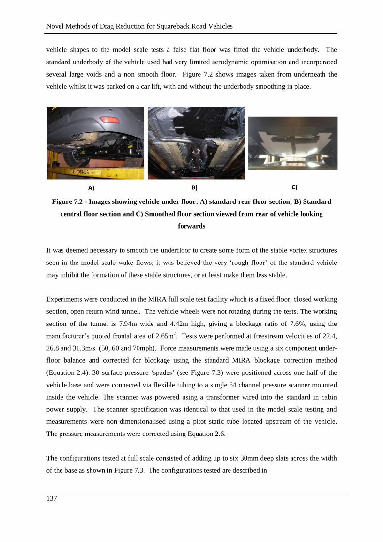
Novel Methods of Drag Reduction for Squareback Road Vehicles
137
vehicle shapes to the model scale tests a false flat floor was fitted the vehicle underbody. The
standard underbody of the vehicle used had very limited aerodynamic optimisation and incorporated
several large voids and a non smooth floor. Figure 7.2 shows images taken from underneath the
vehicle whilst it was parked on a car lift, with and without the underbody smoothing in place.
Figure 7.2 - Images showing vehicle under floor: A) standard rear floor section; B) Standard
central floor section and C) Smoothed floor section viewed from rear of vehicle looking
forwards
It was deemed necessary to smooth the underfloor to create some form of the stable vortex structures
seen in the model scale wake flows; it was believed the very ‘rough floor’ of the standard vehicle
may inhibit the formation of these stable structures, or at least make them less stable.
Experiments were conducted in the MIRA full scale test facility which is a fixed floor, closed working
section, open return wind tunnel. The vehicle wheels were not rotating during the tests. The working
section of the tunnel is 7.94m wide and 4.42m high, giving a blockage ratio of 7.6%, using the
manufacturer’s quoted frontal area of 2.65m2. Tests were performed at freestream velocities of 22.4,
26.8 and 31.3m/s (50, 60 and 70mph). Force measurements were made using a six component under-
floor balance and corrected for blockage using the standard MIRA blockage correction method
(Equation 2.4). 30 surface pressure ‘spades’ (see Figure 7.3) were positioned across one half of the
vehicle base and were connected via flexible tubing to a single 64 channel pressure scanner mounted
inside the vehicle. The scanner was powered using a transformer wired into the standard in cabin
power supply. The scanner specification was identical to that used in the model scale testing and
measurements were non-dimensionalised using a pitot static tube located upstream of the vehicle.
The pressure measurements were corrected using Equation 2.6.
The configurations tested at full scale consisted of adding up to six 30mm deep slats across the width
of the base as shown in Figure 7.3. The configurations tested are described in

Novel Methods of Drag Reduction for Squareback Road Vehicles
138
Table 7.2. and all the configurations were tested with both a smooth under floor and the standard
vehicle underfloor.
Figure 7.3- Full scale test vehicle shown in configuration 1 with pressure ‘spades’ attached to
one half of the vehicle base surface
Table 7.2 - Full scale vehicle configurations
Configuration
Number
Description
0 No slats fitted baseline vehicle configuration
1 6 Slats fitted to the base surface of the vehicle as shown in Figure 7.3
2 5 slats fitted to the base as per configuration 1 but with the upper slat
removed
3 4 slats fitted to the base as per configuration 1 but with the upper slat
removed
4 3 slats fitted to the base as per configuration 3 but with the upper slat
removed
5 2 slats fitted to the base as per configuration 4 but with the upper slat
removed
6 1 slat fitted to the base as per configuration 5 but with the upper slat
removed
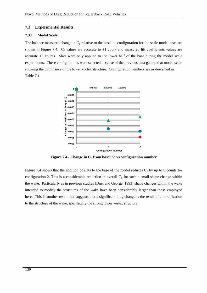
Novel Methods of Drag Reduction for Squareback Road Vehicles
139
7.3 Experimental Results
7.3.1 Model Scale
The balance measured change in Cd relative to the baseline configuration for the scale model tests are
shown in Figure 7.4. Cd values are accurate to ±1 count and measured lift coefficients values are
accurate ±5 counts. Slats were only applied to the lower half of the base during the model scale
experiments. These configurations were selected because of the previous data gathered at model scale
showing the dominance of the lower vortex structure. Configuration numbers are as described in
Table 7.1.
Figure 7.4 - Change in Cd from baseline vs configuration number
Figure 7.4 shows that the addition of slats to the base of the model reduces Cd by up to 8 counts for
configuration 2. This is a considerable reduction in overall Cd for such a small shape change within
the wake. Particularly as in previous studies (Duel and George, 1993) shape changes within the wake
intended to modify the structures of the wake have been considerably larger than those employed
here. This is another result that suggests that a significant drag change is the result of a modification
to the structure of the wake, specifically the strong lower vortex structure.
-0.009
-0.008
-0.007
-0.006
-0.005
-0.004
-0.003
-0.002
-0.001
0
0 1 2
Ch
an
ge i
n C
oefi
cie
nt
of
Dra
g (
Cd
)
Configuration Number
40 m/s 35 m/s 30m/s

Novel Methods of Drag Reduction for Squareback Road Vehicles
140
Figure 7.5 - Change in Cl from baseline
Figure 7.5 shows the vehicle lift coefficient, and the effect of the configuration changes relative to the
baseline configuration. An initial observation is that the Cl values are much more sensitive to
Reynolds number changes than the drag results, however they all follow a trend that with the addition
of slats to the lower half of the base Cl is reduced. This is again a significant change in Cl for a
relatively small shape change, and it supports the theory that disrupting the lower vortex in close
proximity to the base will cause a base pressure increase. It is possible that small modifications at the
rear of the model can cause changes in the stagnation point at the front of the vehicle which could
account for the changes in lift, however looking at the balance of front and rear Cl changes this effect
is only a small percentage of the overall lift change. The rear lift coefficient (Clr) never contributes
less than 80% to the total changes in Cl recorded. This indicates that changes in lift due to movement
of the front stagnation point are small, and the majority of the lift changes occur because of changes to
the wake structure effecting the flow around the rear section of the vehicle.
Figure 7.6 shows a contour plot of base pressure coefficients (Cp) for the baseline configuration (no
slats) and Figure 7.7 shows the Cp distribution when four slats are added (configuration 2). The plots
are oriented such that a view is taken looking from directly behind the model where zero on the x axis
corresponds to the model centreline and zero on the z axis corresponds to the bottom of the model.
-0.035
-0.03
-0.025
-0.02
-0.015
-0.01
-0.005
0
0 1 2
Co
efi
cie
nt
of
Lif
t (C
l)
Configuration Number
40 m/s 35 m/s 30m/s
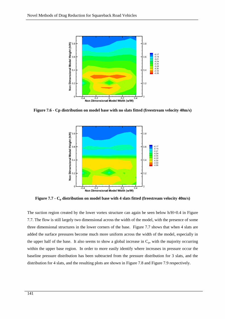
Novel Methods of Drag Reduction for Squareback Road Vehicles
141
Figure 7.6 - Cp distribution on model base with no slats fitted (freestream velocity 40m/s)
Figure 7.7 - Cp distribution on model base with 4 slats fitted (freestream velocity 40m/s)
The suction region created by the lower vortex structure can again be seen below h/H=0.4 in Figure
7.7. The flow is still largely two dimensional across the width of the model, with the presence of some
three dimensional structures in the lower corners of the base. Figure 7.7 shows that when 4 slats are
added the surface pressures become much more uniform across the width of the model, especially in
the upper half of the base. It also seems to show a global increase in Cp, with the majority occurring
within the upper base region. In order to more easily identify where increases in pressure occur the
baseline pressure distribution has been subtracted from the pressure distribution for 3 slats, and the
distribution for 4 slats, and the resulting plots are shown in Figure 7.8 and Figure 7.9 respectively.
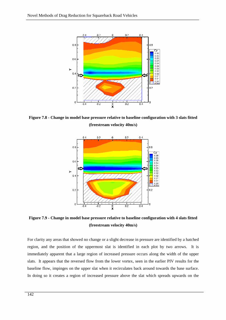
Novel Methods of Drag Reduction for Squareback Road Vehicles
142
Figure 7.8 - Change in model base pressure relative to baseline configuration with 3 slats fitted
(freestream velocity 40m/s)
Figure 7.9 - Change in model base pressure relative to baseline configuration with 4 slats fitted
(freestream velocity 40m/s)
For clarity any areas that showed no change or a slight decrease in pressure are identified by a hatched
region, and the position of the uppermost slat is identified in each plot by two arrows. It is
immediately apparent that a large region of increased pressure occurs along the width of the upper
slats. It appears that the reversed flow from the lower vortex, seen in the earlier PIV results for the
baseline flow, impinges on the upper slat when it recirculates back around towards the base surface.
In doing so it creates a region of increased pressure above the slat which spreads upwards on the
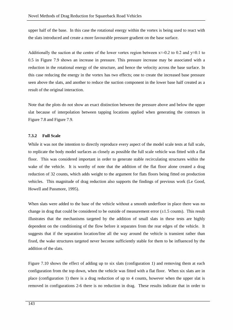
Novel Methods of Drag Reduction for Squareback Road Vehicles
143
upper half of the base. In this case the rotational energy within the vortex is being used to react with
the slats introduced and create a more favourable pressure gradient on the base surface.
Additionally the suction at the centre of the lower vortex region between x≈-0.2 to 0.2 and y≈0.1 to
0.5 in Figure 7.9 shows an increase in pressure. This pressure increase may be associated with a
reduction in the rotational energy of the structure, and hence the velocity across the base surface. In
this case reducing the energy in the vortex has two effects; one to create the increased base pressure
seen above the slats, and another to reduce the suction component in the lower base half created as a
result of the original interaction.
Note that the plots do not show an exact distinction between the pressure above and below the upper
slat because of interpolation between tapping locations applied when generating the contours in
Figure 7.8 and Figure 7.9.
7.3.2 Full Scale
While it was not the intention to directly reproduce every aspect of the model scale tests at full scale,
to replicate the body model surfaces as closely as possible the full scale vehicle was fitted with a flat
floor. This was considered important in order to generate stable recirculating structures within the
wake of the vehicle. It is worthy of note that the addition of the flat floor alone created a drag
reduction of 32 counts, which adds weight to the argument for flats floors being fitted on production
vehicles. This magnitude of drag reduction also supports the findings of previous work (Le Good,
Howell and Passmore, 1995).
When slats were added to the base of the vehicle without a smooth underfloor in place there was no
change in drag that could be considered to be outside of measurement error (±1.5 counts). This result
illustrates that the mechanisms targeted by the addition of small slats in these tests are highly
dependent on the conditioning of the flow before it separates from the rear edges of the vehicle. It
suggests that if the separation location/line all the way around the vehicle is transient rather than
fixed, the wake structures targeted never become sufficiently stable for them to be influenced by the
addition of the slats.
Figure 7.10 shows the effect of adding up to six slats (configuration 1) and removing them at each
configuration from the top down, when the vehicle was fitted with a flat floor. When six slats are in
place (configuration 1) there is a drag reduction of up to 4 counts, however when the upper slat is
removed in configurations 2-6 there is no reduction in drag. These results indicate that in order to
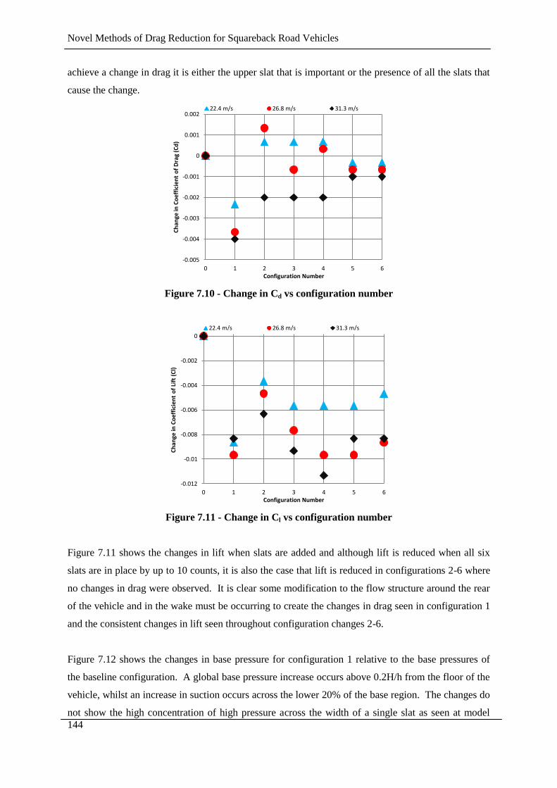
Novel Methods of Drag Reduction for Squareback Road Vehicles
144
achieve a change in drag it is either the upper slat that is important or the presence of all the slats that
cause the change.
Figure 7.10 - Change in Cd vs configuration number
Figure 7.11 - Change in Cl vs configuration number
Figure 7.11 shows the changes in lift when slats are added and although lift is reduced when all six
slats are in place by up to 10 counts, it is also the case that lift is reduced in configurations 2-6 where
no changes in drag were observed. It is clear some modification to the flow structure around the rear
of the vehicle and in the wake must be occurring to create the changes in drag seen in configuration 1
and the consistent changes in lift seen throughout configuration changes 2-6.
Figure 7.12 shows the changes in base pressure for configuration 1 relative to the base pressures of
the baseline configuration. A global base pressure increase occurs above 0.2H/h from the floor of the
vehicle, whilst an increase in suction occurs across the lower 20% of the base region. The changes do
not show the high concentration of high pressure across the width of a single slat as seen at model
-0.005
-0.004
-0.003
-0.002
-0.001
0
0.001
0.002
0 1 2 3 4 5 6
Ch
ange
in C
oef
fici
ent
of
Dra
g (C
d)
Configuration Number
22.4 m/s 26.8 m/s 31.3 m/s
-0.012
-0.01
-0.008
-0.006
-0.004
-0.002
0
0 1 2 3 4 5 6
Ch
ange
in C
oef
fici
ent
of
Lift
(C
l)
Configuration Number
22.4 m/s 26.8 m/s 31.3 m/s

Novel Methods of Drag Reduction for Squareback Road Vehicles
145
scale in Figure 7.8 and Figure 7.9, indicating that the means by which the base pressures are modified
may be different. However, the slats applied are a uniform two dimensional physical addition across
the width of the base, and the resulting changes in base pressure are relatively uniform across the
width of the vehicle.
Figure 7.12 – Change in base pressure (Cp) with 6 slats applied
Examination of the baseline base pressure distribution individually infers a three dimensionality of the
wake flow. When 6 slats are added the individual base pressure distribution for configuration 6 shows
a much more uniform wake flow structure across the width of the base. This phenomena is similar to
the effect seen at model scale where the wake is forced into a more 2 dimensional regime.
7.4 Discussion
A small passive modification has been tested in ¼ scale and full scale wind tunnel tests. The addition
of low profile horizontal slats to the base surface of the scale model produced drag reductions of up to
8 counts and lift reductions of up to 32 counts.
Pressure measurements on the base of the model showed that the interaction of the upper slat with the
recirculating vortex structure in the wake creates a region of increased pressure above the upper slat.
Additionally pressure was recovered in the lower half of the base where the suction regions associated
with the presence of the lower vortex structure are located.

Novel Methods of Drag Reduction for Squareback Road Vehicles
146
At full scale the addition of horizontal slats to the base of the vehicle created drag reductions of 4
counts and lift reductions of 10 counts. Tests conducted without a smooth underfloor showed little or
no change to the lift and drag forces.
In the full scale configurations where force changes were observed pressure measurements showed a
global recovery of base pressure on the base above 0.2H/h from the floor of the vehicle; below
h/H=0.2 a reduction in base pressure was observed. A lack of understanding of the standard full scale
vehicle wake structure means the aerodynamic force changes observed cannot be explained as easily
as the scale model results.
Further investigation is required to fully understand how such a small passive modification can cause
such large force changes observed at full scale. However the changes implemented in the current test
are physically small and located in the wake of a squareback vehicle. Such small modifications in the
wake region would not normally be addressed in an aerodynamic optimisation process since small
changes on the base region of a vehicle have previously be considered unimportant. Any changes in
this region which have previously been effective have required large physical changes, or trailing
edge modifications such as tapering or tripping. With this in mind the reductions in lift and drag as a
result of the configurations tested have been surprisingly large.
The pressure results in Figure 7.8 and Figure 7.9 go some way to explaining how the wake structures
can interact with the base slats to cause body force changes in the scale model tests. However an area
weighted calculation based on the contribution from these small slats shows that the changes in lift
cannot be explained by pressure changes on the horizontal surfaces of the slats themselves, due to
their small horizontal area (as a percentage of the whole vehicle horizontal area).
Further investigation using tappings located on the floor and roof of the model may identify if the lift
reduction using the base slats is caused by pressure changes on the floor of the model by accelerating
flow underneath it. Although the mechanisms involved in creating the changes on the full scale model
are still not understood, it is clear that small changes in the physical architecture of the vehicle/model
relationship can have an effect on where the base slats are effective. This is thought to be due to the
differences in the wake structures found in the two experiments. None of the base slats tested at full
scale without a flat floor had an effect, again highlighting the sensitivity to wake structure changes.
The use of moving ground simulation and rotating wheels will also influence the flow under the
vehicle and the structure of the wake. As a result the optimum position of the slats may be further
influenced by these changes in the test conditions, which may have to be addressed in any vehicle
optimization process.
Novel Methods of Drag Reduction for Squareback Road Vehicles
147
Chapter 8
CONCLUSIONS AND FURTHER WORK
Novel Methods of Drag Reduction for Squareback Road Vehicles
148
8.0 Conclusions and Further Work
It has been shown that reducing Cd of road vehicles can result in significant CO2 emissions reductions
and that new technologies associated with reducing Cd are a worthy field of research.
Many passive and active drag reduction technologies and systems have been reviewed and in the
current thesis a focus has been given to the analysis of a synthetic jet system, steady blowing, and
pulsed blowing for vehicle drag reduction. Early experiments on a 2D cylinder have shown synthetic
jets to work to control flow in laminar, transitional and turbulent boundary layers, however a lack in
Cµ has meant a lack in performance at higher freestream velocities. Although SJ’s offer an attractive
package to create a pulsed disturbance to freestream flows, the practicalities surrounding these
systems currently restricts their application to controlled experimentation at representative Reynold’s
numbers. These practicality limitations also have significant implications for the uptake of the
technology into mainstream road vehicle production. Without significant developments in the
actuators available to enable a ‘flexible’ synthetic jet arrangement the technology will not currently be
applicable to full scale applications. A ‘flexible’ synthetic jet would be defined as an actuator that can
offer significant momentum coefficients at a wide range of actuation frequencies with a low energy
demand. For the reason above synthetic jet actuators were not applied to a road vehicle model.
However the use of steady blowing and pulsed blowing was investigated on a scaled vehicle model.
Before applying the technology to a vehicle model a simple passive optimisation was conducted to
investigate how wake modification can affect base pressure. These investigations highlighted that
wake size and ‘in wake’ flow topologies are the main factors influencing the pressures on the base
surface. The baseline vehicle investigations also revealed that there was no clear shedding patterns
from the upper or lower surfaces, but there was some non-coherent shedding occurring which was
characterised as a Markovian process.
The application of steady blowing at the upper and lower rear edges of the vehicle model create
attractive reductions in drag forces. The reductions are also still viable when the energy demands of
the actuation systems are accounted for. In these experiments the global size of the wake was not
modified as significantly as in the passive optimisation experiments, yet the drag changes were more
significant. The influence of a large lower vortex structure on the base pressures was identified as a
significant mechanism in the creation of the drag savings. In the cases where drag was reduced by
steady blowing, the vorticity found in this lower structure was also reduced. Although there is a net
drag saving the energy requirements of a blowing system would still be significant, requiring the
generation of large mass flow rates and potentially significant storage tanks. These factors all inhibit
the applicability to larger road vehicles. It is suggested that further work could investigate the use of

Novel Methods of Drag Reduction for Squareback Road Vehicles
149
local ducting on the upper and lower surfaces to try to re-direct freestream flow into the wake in the
same manner that the current jets were oriented. Although it is acknowledged that the ducting itself
will create adverse drag savings it may be that these can be compensated for by the positive effects
created in the wake as a result of ‘blowing’. In the current investigation an attempt to reduce the duty
cycle of the jets, a new system was implemented where the jets were pulsed on and off.
The application of pulsed jets found drag reduction was created at low frequency actuation but the
savings were reduced as the frequency was increased. In most cases the drag was actually increased
relative to the baseline case at higher actuation frequencies. After investigation of PIV data it was
found that as frequency is increased so too is the level of vorticity found close to the base. Again a
link was drawn between the vortex strength or vorticity in the large lower vortex structure, and the
changes in base pressures. The reduction in energy demands required to create mass flow for the jets
created by pulsing them will not go far enough to create a clear path for the implementation of the
current technology in standard vehicles.
Although the current work did not find clear drag reductions as a result of pulsing the jet, there are
clearly significant modifications to the flow with the increased frequencies. Specifically as the
frequency is increased wake size is modified more significantly, but more importantly, the vorticity
levels in the wake are increased. It is suggested that further work with the current model could
experiment with higher frequencies to investigate if the trend linking vorticity to increased
frequencies continues, or if another behavioural regime can be created. Either way it is clear that a
reduction in vorticity or a change in the position/size of the lower vortex will have a significant effect
on any changes in base pressure created, and the focus of further work using this model should target
the lower vortex structure. Additionally the current work highlights that vorticity intensity and
location, even within wake flows, can contribute significantly to resultant surface pressures. As a
result it would be of value to re-visit work on wake flows with different shaped vehicle models, using
modern measurement techniques such as PIV, to investigate the presence of vorticity located close to
rearward surfaces, that previously may have been regarded as unimportant.
In other applications, such as underbody diffuser flows, it can be the case that vorticity is a desirable
characteristic, where vorticies are used to create down force. In this application pulsed jets may
create benefits with their ability to increase vorticity.
Knowing the negative effects vorticity can create in wake flows on the current model some small
passive devices were used to test the theory. From the work carried out in Chapter 7.0, it is clear that
wake size manipulation is not the only means of creating base pressure recovery and lift changes, and
detailed optimisation on the base surface may be a means of further aerodynamic optimisation. The

Novel Methods of Drag Reduction for Squareback Road Vehicles
150
flow mechanisms involved in creating the observed changes are still not fully understood and the
transient nature of wake flows makes the understanding a difficult task. However it is clear that with
an optimisation process applied to a specific vehicle shape, drag and lift modification may be possible
if there is the presence of any quasi-stable vortical structures.

Novel Methods of Drag Reduction for Squareback Road Vehicles
151
9.0 References
Ahmed, S.R. and Baumert, W. (1979) The Structure of Wake Flow Behind Road Vehicles, Proc.
ASME-CSME. Conf. Aerodynamics of Transportation.
Ahmed, S.R., Ramm, G. and Faltin, G. (1984) Some Salient Features of the Time Averaged Ground
Vehicle Wake, SAE Technical Paper 840300, doi:10.4271/840300.
Amitay, M. and Glezer, A. (2002) Role of Actuation Frequency in Controlled Flow Reattachment
over a Stalled Airfoil, AIAA Journal Vol. 40, No. 2, February 2002.
Barnard, R.H. (1996) Road Vehicle Aerodynamic Design, Addison Wesley Longman, Harlow.
Bearman, P.W. (1965) Investigation of the flow behind a two-dimensional model with a blunt trailing
edge and fitted with splitter plates, J. Fluid Mech. (1965), vol. 21, part 2, pp. 241-255.
Bearman P.W., a.M.T. (1983) Effect of freestream turbulence on flow around bluff bodies, Prog.
Aerospace Science Vol 20 1983. 97-123.
Beaudoin, J.-F. and Aider, J.-L. (2008) Drag and lift reduction of a 3D bluff body using flaps, Exp
Fluids (2008) 44:491–501.
Béra, J.-C., Michard, M., Sunyach, M. and Comte-Bellot, G. (2000) Changing lift and drag by jet
oscillation: experiments on a circular cylinder with turbulent separation, Eur. J. Mech. B - Fluids 19
(2000) Pg 575–595.
Brazaa, M., Perrina, R. and Hoarau, Y. (2006) Turbulence Properties in the Cylinder Wake at High
Reynolds Numbers, Journal of Fluids and Structures, 22 (2006) Pg 757–771.
Brunn, A. and Nitsche, W. (2006) Active control of turbulent separated flows over slanted surfaces,
International Journal of Heat and Fluid Flow 27 (2006) Pg 748–755.
Carr, G.W., Atkin, P.D. and Sommerville, J. (1994) An empirically-based prediction method for car
aerodynamic lift and side forces, SAE Technical Paper 1994-11-0100.
Ching, W.K. and Ng, M.K. (2006) Markov Chains; Models, Algorithms and Applications, ISBN 978-
0-387-29337-0.
Novel Methods of Drag Reduction for Squareback Road Vehicles
152
Coleman, H.W. and Steele, W.G., (1999) Experimentation and Uncertainty Analysis for
Engineers, 2nd Edition, John Wiley & Sons, Inc., New York, NY.
Cooper, K.R., Bertenyi, T., Dutil, G. and Syms, J. (1998) The Aerodynamic Performance of
Automotive Underbody Diffusers, SAE Technical Paper 980030.
Duel, E.G. and George, A.R. (1993) Measurements in the Unsteady Near Wakes of Ground Vehicle
Bodies, SAE Technical Paper 930298.
Englar, R.J. (1987) The application of circulation control pneumatic technology to powered-lift STOL
aircraft, SAE Technical Paper 872335.
Englar, R.J. (2003) Drag Reduction, Safety Enhancement, and Performance Improvement for Heavy
Vehicles and SUVs Using Advanced Pneumatic Aerodynamic Technology, SAE Technical Paper
2003-01-3378.
Englar, R.J. (2005) Improved Pneumatic Aerodynamics for Drag Reduction, Fuel Economy, Safety
and Stability Increase for Heavy Vehicles, SAE Technical Paper 2005-01-3627.
Geropp, D. and Odentha, H.-J. (2000) Drag Reduction of Motor Vehicles by Active Flow Control
Using the Coanda Effect, Experiments in Fluids 28 (2000) Pg 74-85.
Glezer, A. and Amitay, M. (2002) Synthetic Jets, Annual Review of Fluid Mechanics 34 Pg 503-529.
Glezer, A., Amitay, M. and Honahan, A.M. (2005) Aspects of Low- and High-Frequency Actuation
for Aerodynamic Flow Control, AIAA Journal Vol 43 No.7 July 2005.
Guo, F. and Zhong, S. (2006) A PIV Investigation of the Characteristics of Micro-scale Synthetic Jets,
AIAA paper 2006-3183.
Heisler, H. (2002) Advanced Vehicle Technology, 2nd Edition, Butterworth-Heinemann, Oxford.
Hollis, D. (2004) Particle Image Velocimetry in Gas Turbine Combustor Flow Fields, PhD Thesis,
Loughborough University.
Holman, R. and Utturkar, Y. (2005) Formation Criterion for Synthetic Jets, AIAA Journal Vol. 43,
No. 10, October 2005.
Novel Methods of Drag Reduction for Squareback Road Vehicles
153
Horn, H..N.J..a.W.J. (n.d) 'Rating Mass-related Energy Demand for Vehicles with New Powertrain
Concepts'.
Howell, J. and Le Good, G. (2008) The Effect of Backlight Aspect Ratio on Vortex and Base Drag for
a Simple Car-Like Shape, SAE Technical Paper 2008-01-0737.
Howell, J., Sheppard, A. and Blakemore, A. (2003) Aerodynamic Drag Reduction for a Simple Bluff
Body Using Base Bleed, SAE Technical Paper 2003-01-0995.
Hucho, W.H. (1998) Aerodynamics of Road Vehicles, SAE International.
Jowsey, L. (2008) An Experimental Study of an Automotive Underbody Diffuser, PhD Studies,
Loughborough University.
Keating, A., Shock, R. and Chen, H. (2008) Lattice Boltzmann Simulations of the Unsteady Flow
Behind the Ahmed Body, 2008010740th edition.
Kee, J.D., Kim, M.S. and Lee, B.C. (2001) The COANDA Flow Control and Newtonian Concept
Approach to Acheive Drag Reduction of Passenger Vehicles, SAE Technical Paper 2001-01-1267.
Khalighi, B., Zhang, S. and Koromilas, C. (2001) 'Experimental and Computational Study of
Unsteady Wake Flow Behind a Bluff Body with a Drag Reduction Device'.
Kim, Y.H. and Gary, K.P. (2006) Optimization of a Rectangular Orifice Synthetic Jet Generator,
AIAA paper 2006-2862.
Kourta, A. (2008) Separated Flow Control and Actuators Development, Presentation, KATnet II,
Separation and Control Workshop, 1-3 April 2008, ONERA, Toulouse, France. Web link:
http://www.kat-net.net/publications/data/64_20080423_%5B5%5D_kourta.pdf.
Kowata, S., Ha, J., Yoshioka, S., Kato, T. and Kohama, Y. (2008) Drag Force Reduction of a Bluff-
Body with an Underbody Slant and Rear Flaps, SAE Technical Paper 2008-01-2599.
Lanser, W.R. and Ross, J.C. (1991) Aerodynamic Performance of a Drag Reduction Device on a Full-
Scale Tractor/Trailer, SAE Technical Paper 912125.
Le Good, G.M., Howell, J.P. and Passmore, M.A. (1995) On-road aerodynamic drag measurements
compared with wind tunnel data, SAE Paper 950627.
Novel Methods of Drag Reduction for Squareback Road Vehicles
154
Leclerc, C. and Levallois, E. (2006) Aerodynamic Drag Reduction by Synthetic Jet: A 2D Numerical
Study Around a Simplified Car, AIAA Flow Control Conference Paper 2006-3337.
Lockerby, D.A. and Carpenter, P.W. (2004) Modeling and Design of Microjet Actuators, AIAA
Journal Vol. 42, No. 2, February 2004.
Mason, W.T. and Beebe, P.S. (1976) The Drag Related Flow Field Characteristics of Trucks and
Buses, Aerodynamic Drag Mechanics of Bluff Bodies and Road Vehicle Symposium, held at General
Motors Research Laboratory, Warren, Michigan, September 27-28, 1976.
McKormick, D.C. (2000) Boundary Layer Separation Control with Directed Synthetic Jets, AIAA
paper 2000-0519.
Mittal, R. and Rampunggoon, P. (2002) On the virtual aeroshaping effect of synthetic jets, Physics of
Fluids Volume 14, Number 4 April 2002.
Modi, V.J. (1997) Moving Surface Boundary-Layer Control: a Review, Journal of Fluids and
Structures (1997) 11 Pg 627-663.
Modi, V.J. and Ying, B. (1990) Boundary-Layer Control of Bluff Bodies Through Momentum
Injection, SAE Technical Paper 902225.
Pastoor, M., Henning, L., Noack, B.R., King, R. and Tadmor, G. (2008) Feedback shear layer control
for bluff body drag reduction, J. Fluid Mech., vol. 608, pp. 161–196.
Peterson, R.L. (1981) Drag Reduction Obtained by the Addition of a Boattail to a Box Shaped
Vehicle, NASA Contractor Report 163113.
Plackett, L. (2009) Experimental analysis of impulsively started jet flow, Loughborough University,
Masters Thesis.
Raffel, M., Willert, C.E., Wereley, S.T. and Kompenhans, J. (2007) Particle Image Velocimetry - A
Practicle Guide, Springer ISBN 978-3-540-72308-0.
Ribaldone, E.. (n.d) 'Application of mulit-objective optimization to the aerodynamic development of
passenger vehicles at FIAT'.
Novel Methods of Drag Reduction for Squareback Road Vehicles
155
Roshko, A. (1961) Experiments on the Flow Past a Circular Cylinder at Very High Reynolds Number,
Journal of Fluid Mechanics 10 Pg 345-356.
Roumeas, M. (2006) Contribution à l'analyse et au contrôle des sillages de corps épais par aspiration
ou soufflage continu, PhD Thesis Institut de Mécanique des Fluides de Toulouse - IMFT (Toulouse,
France).
Rouméas, M., Gilliéron, P. and Kourta, A. (2006) Analyze and Control of the Near-Wake Flow over a
Square Back Geometry, AIAA paper 2006-3336.
Schrefl, M. (n.d) 'The Audi A1 – Aerodynamics and Aeroacoustics'.
Schultz, S. (2010) Aerodynamics of Modern Sport Utility Vehicles, Technical Paper, 8th MIRA
International Vehicle Aerodynamics Conference.
Sharma, R.N. (2006) An Analytical Model for Synthetic Jet Actuation, AIAA paper 2006-3035.
Smith, B.L. and Glezer, A. (2002) Jet Vectoring Using Synthetic Jets, J. Fluid Mech. Vol. 458 Pg 1-
34.
TrailerTail (2007) http://www.atdynamics.com/trailertail.htm.
Verzicco, R., Fatica, M., Iaccarino, G. and Moin, P. (2002) Large Eddy Simulation of a Road Vehicle
with Drag-Reduction Devices, AIAA Journal Vol. 40, No. 12.
Wong, D.T.M. and Mair, W.A. (1983) Boat-Tailed Afterbodies of Square Section as Drag Reduction
Devices, Journal of Wind Engineering and Industrial Aerodynamics, 12 (1983).