What is DFA - RiskNET

INTRODUCTION TO DYNAMIC FINANCIAL ANALYSIS

ROGER KAUFMANN, ANDREAS GADMER, AND RALF KLETT

Abstract. In the last few years we have witnessed growing interest in Dynamic Finan-cial Analysis (DFA) in the nonlife insurance industry. DFA combines many economicand mathematical concepts and methods. It is almost impossible to identify and de-scribe a unique DFA methodology. There are some DFA software products for nonlifecompanies available in the market, each of them relying on its own approach to DFA.Our goal is to give an introduction into this field by presenting a model framework com-prising those components many DFA models have in common. By explicit reference tomathematical language we introduce an up-and-running model that can easily be im-plemented and adjusted to individual needs. An application of this model is presentedas well.

1. What is DFA

1.1. Background. In the last few years, nonlife insurance corporations in the US, Canadaand also in Europe have experienced, among other things, pricing cycles accompanied byvolatile insurance profits and increasing catastrophe losses contrasted by well performingcapital markets, which gave rise to higher realized capital gains. These developmentsimpacted shareholder value as well as the solvency position of many nonlife companies.One of the key strategic objectives of a joint stock company is to satisfy its owners byincreasing shareholder value over time. In order to achieve this goal it is necessary toget an understanding of the economic factors driving shareholder value and the cost ofcapital. This does not only include identifying the factors but investigating their randomnature and interrelations to be able to quantify earnings volatility. Once this has beendone various business strategies can be tested in respect of meeting company objectives.There are two primary techniques in use today to analyze financial effects of different

entrepreneurial strategies for nonlife insurance companies over a specific time horizon.The first one – scenario testing – projects business results under selected deterministicscenarios into the future. Results based on such a scenario are valid only for this spe-cific scenario. Therefore, results obtained by scenario testing are useful only insofar asthe scenario was correct. Risks associated with a specific scenario can only roughly bequantified. A technique overcoming this flaw is stochastic simulation, which is knownas Dynamic Financial Analysis (DFA) when applied to financial cash flow modelling ofa (nonlife) insurance company. Thousands of different scenarios are generated stochas-tically allowing for the full probability distribution of important output variables, likesurplus, written premiums or loss ratios.

Date: April 26, 2001.Key words and phrases. Nonlife insurance, Dynamic Financial Analysis, Asset/Liability Management,

stochastic simulation, business strategy, efficient frontier, solvency testing, interest rate models, claims,reinsurance, underwriting cycles, payment patterns.

The article is partially based on a diploma thesis written in cooperation with Zurich Financial Services.Further research of the first author was supported by Credit Suisse Group, Swiss Re and UBS AG throughRiskLab, Switzerland.

1

2 R. KAUFMANN, A. GADMER, AND R. KLETT

1.2. Fixing the Time Period. The first step to compare different strategies is to fixa time horizon they should apply to. On the one hand we would like to model over aslong a time period as possible in order to see the long-term effects of a chosen strategy.In particular, effects concerning long-tail business only appear after some years and canhardly be recognized in the first few years. On the other hand, simulated values becomemore unreliable the longer the projection period, due to accumulation of process andparameter risk over time. A projection period of five to ten years seems to be a reasonablechoice. Usually the time period is split into yearly, quarterly or monthly sub periods.

1.3. Comparison to ALM in Life Insurance. A DFA model is a stochastic modelof the main financial factors of an insurance company. A good model should simulatestochastically the asset elements, the liability elements and also the relationships betweenboth types of random factors. Many traditional ALM-approaches (ALM=Asset-LiabilityManagement) in life insurance considered the liabilities as more or less deterministicdue to their low variability (see for example Wise [43] or Klett [25]). This approachwould be dangerous in nonlife where we are faced with much more volatile liability cashflows. Nonlife companies are highly sensitive to inflation, macroeconomic conditions,underwriting movements and court rulings, which complicate the modelling process whilesimultaneously making results less certain than for life insurance companies. In nonlifeboth the date of occurrence and the size of claims are uncertain. Claim costs in nonlifeare inflation sensitive, whereas they are expressed in nominal terms for many traditionallife insurance products. In order to cope with the stochastic nature of nonlife liabilitiesand assets, their number and their complex interactions, we have to rely on stochasticsimulations.

1.4. Objectives of DFA. DFA is not an academic discipline per se. It borrows manywell-known concepts and methods from economics and statistics. It is part of the finan-cial management of the firm. As such it is committed to management of profitability andfinancial stability (risk control function of DFA). While the first task aims at maximiz-ing shareholder value, the second one serves maintaining customer value. Within thesetwo seemingly conflicting coordinates DFA tries to facilitate and help justify or explainstrategic management decisions with respect to

• strategic asset allocation,• capital allocation,• performance measurement,• market strategies,• business mix,• pricing decisions,• product design,• and others.

This listing suggests that DFA goes beyond designing an asset allocation strategy. In fact,portfolio managers will be affected by DFA decisions as well as underwriters. Concreteimplementation and application of a DFA model depends on two fundamental and closelyrelated questions to be answered beforehand:

1. Who is the primary beneficiary of a DFA analysis (shareholder, management,policyholders)?

2. What are the company individual objectives?

INTRODUCTION TO DYNAMIC FINANCIAL ANALYSIS 3

✲ risk

✻

return

Figure 1.1. Efficient frontier.

The answer to the first question determines specific accounting rules to be taken intoaccount as well as scope and detail of the model. For example, those companies onlyinterested in getting a tool for enhancing their asset allocation on very high aggregationlevel will not necessarily target a model that emphasizes every detail of simulating liabilitycash flows. Smith [39] has pointed out that making money for shareholders has not beenthe primary motivation behind developments in ALM (or DFA). Furthermore, relyingon the Modigliani-Miller theorem (see Modigliani and Miller [34]) he put forward thehypothesis that a cost benefit analysis of asset/liability studies might reveal that costsfall on shareholders but benefits on management or customers. Our general conclusionis that company individual objectives – in particular with respect to the target group –have to be identified and formulated before starting the DFA analysis.

1.5. Analyzing DFA Results Through Efficient Frontiers. Before using a DFAmodel, management has to choose a financial or economic measure in order to assessparticular strategies. The most common framework is the efficient frontier concept widelyused in modern portfolio theory going back to Markowitz [32]. First, a company hasto choose a return measure (e.g. expected surplus) and a risk measure (e.g. expectedpolicyholder deficit, see Lowe and Stanard [30], or worst conditional mean as a coherentrisk measure, see Artzner, Delbaen, Eber and Heath [2] and [3]). Then the measuredrisk and return of each strategy can be plotted as shown in Figure 1.1. Each strategyrepresents one spot in the risk-return diagram. A strategy is called efficient if there is noother one with lower risk at the same level of return, or higher return at the same levelof risk. For each level of risk there is a maximal return that cannot be exceeded, givingrise to an efficient frontier. But the exact position of the efficient frontier is unknown.There is no absolute certainty whether a strategy is really efficient or not. DFA is notnecessarily a method to come up with an optimal strategy. DFA is predominantly a toolto compare different strategies in terms of risk and return. Unfortunately, comparisonof strategies may lead to completely different results as we change the return or riskmeasure. A different measure may lead to a different preferred strategy. This will beillustrated in Section 4.


Though efficient frontiers are a good means of communicating the results of DFA be-cause they are well-known, some words of criticism are in place. Cumberworth, Hitchcox,McConnell and Smith [10] have pointed out that there are pitfalls related to efficient fron-tiers one has to be aware of. They criticize that typical efficient frontier uses risk measuresthat mix together systematic risk (non-diversifiable by shareholders) and non-systematicrisk, which blurs the shareholder value perspective. In addition to that, efficient frontiersmight give misleading advice if they are used to address investment decisions once theconcept of systematic risk has been factored into the equation.

1.6. Solvency Testing. A concept closely related to DFA is solvency testing where thefinancial position of the company is evaluated from the perspective of the customers.The central idea is to quantify in probabilistic terms whether the company will be ableto meet its commitments in the future. This translates into determining the necessaryamount of capital given the level of risk the company is exposed to. For example, doesthe company have enough capital to keep the probability of loosing α ·100% of its capitalbelow a certain level for the risks taken? DFA provides a whole probability distributionof surplus. For each level α the probability of loosing α · 100% can be derived from thisdistribution. Thus DFA serves as a solvency testing tool as well. More information aboutsolvency testing can be found in Schnieper [37] and [38].

1.7. Structure of a DFA Model. Most DFA models consist of three major parts, asshown in Figure 1.2. The stochastic scenario generator produces realizations of randomvariables representing the most important drivers of business results. A realization of arandom variable in the course of simulation corresponds to fixing a scenario. The seconddata source consists of company specific input (e.g. mean severity of losses per line ofbusiness and per accident year), assumptions regarding model parameters (e.g. long-termmean rate in a mean reverting interest rate model), and strategic assumptions (e.g. in-vestment strategy). The last part, the output provided by the DFA model, can thenbe analyzed by management in order to improve the strategy, i.e. make new strategicassumptions. This can be repeated until management is convinced by the superiority ofa certain strategy. As pointed out in Cumberworth, Hitchcox, McConnell and Smith [10]interpretation of the output is an often neglected and non-appreciated part in DFA mod-elling. For example, an efficient frontier leaves us still with a variety of equally desirablestrategies. At the end of the day management has to decide for only one of them andselection of a strategy based on preference or utility functions does not seem to providea practical solution in every case.

2. Stochastically Modelled Variables

A very important step in the process of building an appropriate model is to identifythe key random variables affecting asset and liability cash flows. Afterwards it has tobe decided whether and how to model each or only some of these factors and the re-lationships between them. This decision is influenced by considerations of a trade-offbetween improvement of accuracy versus increase in complexity which is often felt beingequivalent to a reduction of transparency.The risks affecting the financial position of a nonlife insurer can be categorized in

various ways. For example, pure asset, pure liability and asset/liability risks. We believethat a DFA model should at least address the following risks:

• pricing or underwriting risk (risk of inadequate premiums),


stochastic scenario generator

input: - historical data

- model parameters

- strategic assumptions

output

analyze output,revise strategy

?

�

�

6

Figure 1.2. Main structure of a DFA model.

• reserving risk (risk of insufficient reserves),• investment risk (volatile investment returns and capital gains),• catastrophes.

We could have also mentioned credit risk related to reinsurer default, currency risk andsome more. For a recent, detailed DFA discussion of the possible impact of exchange rateson reinsurance contracts see Blum, Dacorogna, Embrechts, Neghaiwi and Niggli [5]. Acritical part of a DFA model are the interdependencies between different risk categories,in particular between risks associated with the asset side and those belonging to liabilities.The risk of company losses triggered by changes in interest rates is called interest raterisk. We will come back to the question of modelling dependencies in Section 5.1. Ourchoice of company relevant random variables is based on the categorization of risks shownbefore.A key module of a DFA model is an interest rate generator. Many models assume

that interest rates will drive the whole model as displayed for example in Figure 4.1. Aninterest rate generator – or economic scenario generator as it is often called to emphasizethe far reaching economic impact of interest rates – is necessary in order to be able totackle the problem of evaluating interest rate risk. Moreover, nonlife insurance companiesare strongly exposed to interest rate behavior due to generally large investments in fixedincome assets. In our model implementation we assumed that interest rates were stronglycorrelated with inflation, which itself influenced future changes in claim size and claimfrequency. On the other hand, both of these factors affected (future) premium rates.Furthermore, we assumed correlation between interest rates and stock returns, which aregenerally an important component of investment returns.On the liability side, we explicitly considered four sources of randomness: non-catastro-

phe losses, catastrophe losses, underwriting cycles, and payment patterns. We simulatedcatastrophes separately due to quite different statistical behaviour of catastrophe andnon-catastrophe losses. In general the volume of empirical data for non-catastrophe lossesis much bigger than for catastrophe losses. Separating the two led to more homogeneousdata for non-catastrophe losses, which made fitting the data by well-known (right skewed)distributions easier. Also, our model implementation allowed for evaluating reinsurance


programs. Testing different deductibles or limits is only possible if the model is able togenerate sufficiently large individual losses. In addition, we currently experience a rapiddevelopment of a theory of distributions for extremal events (see Embrechts, Kluppelbergand Mikosch [16], and McNeil [33]). Therefore, we considered the separate modelling ofcatastrophe and non-catastrophe losses as most appropriate. For each of these two groupsthe number and the severity of claims were modelled separately. Another approachwould have been to integrate the two kinds of losses by using heavy-tailed claim sizedistributions.Underwriting cycles are an important characteristic of nonlife companies. They reflect

market and macroeconomic conditions and they are one of the most important factorsaffecting business results. Therefore, it is useful to have them included in a DFA modelset-up.Losses are not only characterized by their (ultimate) size but also by their piecewise

payment over time. This property increases the uncertainties of the claims process by in-troducing the time value of money and future inflation considerations. As a consequence,it is necessary not only to model claim frequency and severity but the uncertainties in-volved in the settlement process as well. In order to allow for reserving risk we usedstochastic payment patterns as a means of estimating loss reserves on a gross and on anet basis.In the abstract we pointed out that our intention was to present a DFA model frame-

work. In concrete terms, this means that we present a model implementation that wefound useful to achieve part of the goals outlined in Section 1.4. We do not claim that thecomponents introduced in the remaining part of the paper represent a high class standardof DFA modelling. For each of the DFA components considered there are numerous alter-natives, which might turn out to be more appropriate in particular situations. Providinga model framework means to present our model as a kind of suggested reference pointthat can be adjusted or improved individually.

2.1. Interest Rates. Following Daykin, Pentikainen and Pesonen [15, p. 231] we assumestrong correlation between general inflation and interest rates. Our primary stochasticdriver is the (instantaneous) short-term interest rate. This variable determines bondreturns across all maturities as well as general inflation and superimposed inflation byline of business.An alternative to the modelling of interest and inflation rates as outlined in this section

and probably well-known to actuaries is the Wilkie model, see Wilkie [42], or Daykin,Pentikainen and Pesonen [15, pp. 242–250].

2.1.1. Short-Term Interest Rate. There are many different interest rate models used byfinancial economists. Even the literature offering surveys of interest rate models hasgrown considerably. The following references represent an arbitrary selection: Ahlgrim,D’Arcy and Gorvett [1], Musiela and Rutkowski [35, pp. 281–302] and Bjork [4]. The finalchoice of a specific interest rate model is not straightforward, given the variety of existingmodels. It might be helpful to post some general features of interest rate movements,which we took from Ahlgrim, D’Arcy and Gorvett [1]:

1. Volatility of yields at different maturities varies.2. Interest rates are mean-reverting.3. Rates at different maturities are positively correlated.4. Interest rates should not be allowed to become negative.


5. The volatility of interest rates should be proportional to the level of the rate.

In addition to these characteristics there are some practical issues raised by Rogers [36].According to Rogers an interest rate model should be

• flexible enough to cover most situations arising in practice,• simple enough that one can compute answers in reasonable time,• well-specified, in that required inputs can be observed or estimated,• realistic, in that the model will not do silly things.

It is well-known that an interest rate model meeting all the criteria mentioned doesnot exist. We decided to rely on the one-factor Cox–Ingersoll–Ross (CIR) model. CIRbelongs to the class of equilibrium based models where the instantaneous rate is modelledas a special case of an Ornstein–Uhlenbeck process:

(2.1) dr = κ (θ − r) dt+ σ rγ dZ ,

By setting γ = 0.5 we arrive at CIR also known as the square root process

(2.2) drt = a (b− rt) dt+ s√rt dZt ,

where

rt = instantaneous short-term interest rate,

b = long-term mean,

a = constant that determines the speed of reversion

of the interest rate toward its long-run mean b,

s = volatility of the interest rate process,

(Zt) = standard Brownian motion.

CIR is a mean-reverting process where the short rate stays almost surely positive. More-over, CIR allows for an affine model of the term structure making the model analyticallymore tractable. Nevertheless, some studies have shown (see Rogers [36]) that one-factormodels in general do not satisfactorily fit empirical data and restrict term structure dy-namics. Multifactor models like Brennan and Schwartz [6] or Longstaff and Schwartz [29]or whole yield approaches like Heath–Jarrow–Morton [20] have proven to be more appro-priate in this respect. But this comes at the price of being much more involved froma theoretical and a practical implementation point of view. Our decision for CIR wasmotivated by practical considerations. It is an easy to implement model that gave usreasonable results when applied to US market data. Moreover, it is a standard modeland in widespread use, in particular in the US.Actually, we are interested in simulating the short rate dynamics over the projection

period. Hence, we discretized the mean reverting model (2.2) leading to

(2.3) rt = rt−1 + a (b− rt−1) + s√rt−1 Zt ,

where

rt = the instantaneous short-term interest rate

at the beginning of year t,

Zt ∼ N (0, 1), Z1, Z2, . . . i.i.d.,

a, b, s as in (2.2).


Cox, Ingersoll and Ross [9] have shown that rates modelled by (2.2) are positive almostsurely. Although it is hard for the short rate process to go negative in the discrete versionof the last equation the probability is not zero. To be sure we changed equation (2.3) to

(2.4) rt = rt−1 + a (b− rt−1) + s√rt−1

+ Zt .

A generalization of CIR is given by the following equation, where setting g = 0.5 yieldsagain CIR:

(2.5) rt = rt−1 + a (b− rt−1) + s (rt−1+)g Zt .

This general version provides more flexibility in determining the degree of dependencebetween conditional volatility of interest rate changes and the level of interest rates.The question of what an appropriate level for g might be leads to the field of model

calibration which we will encounter at several places within DFA modelling. In fact, theproblem plays a dominant role in DFA tempting many practitioners to state that DFAis all about calibration. Calibrating an interest rate model of the short rate refers todetermining parameters – a, b, s and g in equation (2.5) – so as to ensure that modelledspot rates (based on the instantaneous rate) correspond to empirical term structuresderived from traded financial instruments. Bjork [4] calls the procedure to achieve thisinversion of the yield curve. However, the parameters can not be uniquely determinedfrom an empirical term structure and term structure of volatilities resulting in a non-perfect fit. This is a general feature of equilibrium interest rate models. Whereas this isa critical point for valuing interest rate derivatives, the impact on long-term DFA resultsmay be limited.With regard to calibrating the inflation model it should be mentioned that building

models of inflation based on historical data may be a feasible approach. But it is unclearwhether the future evolution of inflation will follow historical patterns: DFA output willprobably reflect the assumptions with regard to inflation dynamics. Consequently, someattention needs to be paid to these assumptions. Neglecting this is a common pitfall ofDFA modelling. In order to allow for stress testing of parameter assumptions, the modelshould not only rely on historical data but on economic reasoning and actuarial judgmentof future development as well.

2.1.2. Term Structure. Based on equation (2.2) we calculated the prices F (t, T, (rt)) beingin place at time t of zero-coupon bonds paying 1 monetary unit at time of maturity t+T ,as

(2.6) F (t, T, (rt)) = EQ [e− ∫ T

0 rt+s ds|rt] = elog AT −rt BT ,

where

AT =( 2Ge(a+G) T/2

(a+G) (eGT − 1) + 2G

)2ab/s2

,

BT =2(eGT − 1)

(a +G) (eGT − 1) + 2G,

G =√a2 + 2s2 .

A proof of this result can be found in Lamberton and Lapeyre [27, pp. 129–133]. Note,that the expectation operator is taken with respect to the martingale measure Q assumingthat equation (2.2) is set up under the martingale measure Q as well. The continuously


compounded spot rates Rt,T at time t derived from equation (2.6) determine the modelledterm structure of zero-coupon yields at time t:

(2.7) Rt,T = − logF (t, T, (rt))

T=rtBT − logAT

T,

where T is the time to maturity.

2.1.3. General Inflation. Modelling loss payments requires having regard to inflation.Following our introductory remark to Section 2.1 we simulated general inflation it byusing the (annualized) short-term interest rate rt. We did this by using a linear regressionmodel on the short-term interest rate:

(2.8) it = aI + bI rt + σ

I εIt ,

where

εIt ∼ N (0, 1), εI1, εI2, . . . i.i.d.,

aI, bI, σI: parameters that can be estimated by

regression, based on historical data.

The index I stands for general inflation.

2.1.4. Change by Line of Business. Lines of business are affected differently by generalinflation. For example, car repair costs develop differently over time than business inter-ruption costs. Claims costs for specific lines of business are strongly affected by legislativeand court decisions, e.g. product liability. This gives rise to so-called superimposed infla-tion, adding to general inflation. More on this can be found in Daykin, Pentikainen andPesonen [15, p. 215] and Walling, Hettinger, Emma and Ackerman [41].To model the change in loss frequency δF

t (i.e. the ratio of number of losses divided bynumber of written exposure units), the change in loss severity δX

t , and the combinationof both of them, δP

t , we used the following formulas:

δFt = max (aF + bF it + σ

F εFt ,−1),(2.9)

δXt = max (aX + bX it + σ

X εXt ,−1),(2.10)

δPt = (1 + δF

t ) (1 + δXt )− 1,(2.11)

where

εFt ∼ N (0, 1), εF1 , εF2 , . . . i.i.d.,

εXt ∼ N (0, 1), εX1 , εX2 , . . . i.i.d., ε

Ft1, εXt2 independent ∀ t1, t2 ,

aF , bF , σF , aX , bX , σX: parameters that can be estimated by

regression, based on historical data.

The variable δPt represents changes in loss trends triggered by changes in inflation rates.

δPt is applied to premium rates as will be explained in Section 3, see (3.2). Its constructionthrough (2.11) ensures correlation of aggregate loss amounts and premium levels that canbe traced back to inflation dynamics.The technical restriction of setting δF

t and δXt to at least −1 was necessary to avoid

negative values for numbers of losses and loss severities.


We modelled changes in loss frequency dependent on general inflation because empiricalobservations revealed that under specific economic conditions (e.g. when inflation is high)policyholders tend to report more claims in certain lines of business.The corresponding cumulative changes δF,c

t and δX,ct can be calculated by

δF,ct =

t∏s=t0+1

(1 + δFs ),(2.12)

δX,ct =

t∏s=t0+1

(1 + δXs ),(2.13)

wheret0 + 1 = first year to be modelled.

2.2. Stock Returns. The major asset classes of a nonlife insurance company comprisefixed income type assets, stocks and real estate. Here, we confine ourselves to a descriptionof the model employed for stocks. Modelling stocks can start either with concentratingon stock prices or stock returns (although both methods should turn out to be equivalentin the end). We followed the last approach since we could rely on a well establishedtheory relating stock returns and the risk-free interest rate: the Capital Asset PricingModel (CAPM) going back to Sharpe–Lintner, see for example Ingersoll [22].In order to apply CAPM we needed to model the return of a portfolio that is supposed

to represent the stock market as a whole, the market portfolio. Assuming a significantcorrelation between stock and bond prices and taking into account multi-periodicity of aDFA model we came up with the following linear model for the stock market return inprojection year t conditional on the one-year spot rate Rt,1 at time t.

(2.14) E [rMt |Rt,1] = a

M + bM (eRt,1 − 1) ,

where

eRt,1−1 = risk-free return, see (2.7),

aM , bM = parameters that can be estimated by regression,

based on historical data and economic reasoning.

Since we modelled sub periods of length one year, we conditioned on the one-year spotrate. Note that rM

t must not be confused with the instantaneous short-term interestrate rt in CIR. Note also that a negative value of bM means that increasing interest ratesentail expected stock prices falling.Now we can apply the CAPM formula to get the conditional expected return on an

arbitrary stock S:

(2.15) E [rSt |Rt,1] = (eRt,1 − 1) + βS

t

(E [rM

t |Rt,1]− (eRt,1 − 1)),

where

eRt,1−1 = risk-free return,

rMt = return on the market portfolio,

βSt = β-coefficient of stock S

=Cov (rS

t , rMt )

Var (rMt )

.


If we assume a geometric Brownian Motion for the stock price dynamics we get a lognor-mal distribution for 1 + rS

t :

(2.16) 1 + rSt ∼ lognormal (µt, σ

2), rS1 , r

S2 , . . . independent,

with µt chosen to yield

mt = eµt+σ2/2,

where

mt = 1 + E [rSt |Rt,1], see (2.15),

σ2 = estimated variance of logarithmic historical stock returns.

Again, we would like to emphasize that our method of modelling stock returns representsonly one out of many possible approaches.

2.3. Non-Catastrophe Losses. Usually, non-catastrophe losses of various lines of busi-ness develop quite differently compared to catastrophe losses, see also the introductoryremarks of Section 2. Therefore, we modelled non-catastrophe and catastrophe lossesseparately and per line of business. For simplicity’s sake, we will drop the index denotingline of business in this section.Experience shows that loss amounts depend also on the age of insurance contracts. The

aging phenomenon describes the fact that the loss ratio – i.e. the ratio of (estimated) totalloss divided by earned premiums – decreases when the age of policy increases. For thisreason we divided insurance business into three classes, as proposed by D’Arcy, Gorvett,Herbers, Hettinger, Lehmann and Miller [13]:

• new business (superscript 0),• renewal business – first renewal (superscript 1), and• renewal business – second and subsequent renewals (superscript 2).

More information about the aging phenomenon can be found in D’Arcy and Doherty [11]and [12], Feldblum [19], and in Woll [44].Disregarding the time of incremental loss payment for the moment, the two main

stochastic factors affecting total claim amount are: number of losses and severity oflosses, see for instance Daykin, Pentikainen and Pesonen [15]. The choice of a specificclaim number and claim size distribution depends on the line of business and is the resultof fitting distributions to empirical data requiring foregoing adjustments of historicalloss data. In this section we shall demonstrate our model of non-catastrophe losses byreferring to a negative binomial (claim number) and a gamma (claim size) distribution.

To simulate loss numbers N jt and mean loss severities Xj

t = 1

Njt

∑Njt

i=1Xjt (i) for period t

and renewal category j we utilized mean values µF,j, µX,j and standard deviations σF,j,σX,j of historical data for loss frequencies and mean loss severities. We took also intoaccount inflation and written exposure units. Because loss frequencies behave more stablethan loss numbers, we used estimations of loss frequencies instead of relying on estimatesof loss numbers.As an example of a distribution for claim numbers N j

t we consider the negative binomialdistribution with mean mN,j

t and variance vN,jt . Generally, we reserved the variables m

and v for mean and variance of different factors. These factors were referred by attaching


a superscript (N,X, Y, . . . ) to m or v:

N jt ∼ NB (a, p), j = 0, 1, 2 ,

N j1 , N

j2 , . . . independent,

(2.17)

with a and p chosen to yield

mN,jt = E [N j

t ] =a (1− p)p

,

vN,jt = Var (N j

t ) =a (1− p)p2

,

(2.18)

where

mN,jt = wj

t µF,j δF,c

t ,

vN,jt = (wj

t σF,j δF,c

t )2,

wjt = written exposure units; introduced in more detail

and modelled in (3.3),

µF,j = estimated frequency, based on historical data,

σF,j = estimated standard deviation of frequency,

based on historical data,

δF,ct = cumulative change in loss frequency, see (2.12).

Negative binomial distributed variables N exhibit over-dispersion: Var(N ) ≥ E[N ]. Con-

sequently, this distribution yields a reasonable model only if vN,jt ≥ mN,j

t .Historical data are a good basis to calibrate this model as long as there had been no

significant structural changes within a line of business in prior years. Otherwise, explicitconsideration of exposure data may be a better basis for calibrating the claims process.In the following we will present an example of a claim size distribution for high fre-

quency, low severity losses. Due to the fact that the density function of the gammadistribution decreases exponentially under appropriate choice of parameters it is a distri-bution serving our purposes well:

Xjt ∼ Gamma(α, θ), j = 0, 1, 2 ,

Xj1 , X

j2 , . . . independent,

(2.19)

with α and θ chosen to yield

mX,jt = E [Xj

t ] = α θ ,

vX,jt = Var (Xj

t ) = α θ2,


where

mX,jt = µX,j δX,c

t ,

vX,jt = (σX,j δX,c

t )2/δF,ct ,

µX,j = estimated mean severity, based on historical data,

σX,j = estimated standard deviation, based on historical data,

δX,ct = cumulative change in loss severity, see (2.13),

δF,ct = cumulative change in loss frequency, see (2.12).

By multiplying the number of losses with the mean severity, we got the total (non-catastrophic) loss amount in respect of a certain line of business:

∑2j=0N

jt X

jt .

2.4. Catastrophes. We are turning now to losses triggered by catastrophic events likewindstorm, flood, hurricane, earthquake, etc. In Section 2 we mentioned that we couldhave integrated non-catastrophic and catastrophic losses by using heavy-tailed distri-butions, see Embrechts, Kluppelberg and Mikosch [16]. Nevertheless, we decided forseparate modelling, see our reasons given in Section 2.There are different ways of modelling the number of catastrophes, e.g. negative bino-

mial, poisson, or binomial distribution with mean mM and variance vM . We assumedthat there were no trends in the number of catastrophes:

Mt ∼ NB, Pois, Bin, . . . (mean mM , variance vM),

M1,M2, . . . i.i.d.,(2.20)

where

mM = estimated number of catastrophes, based on historical data,

vM = estimated variance, based on historical data.

Contrary to the modelling of non-catastrophe losses, we simulated the total (economic)loss (i.e. not only the part the insurance company in consideration has to pay) for eachcatastrophic event i ∈ {1, . . . ,Mt} separately. Again, there are different probabilitydistributions, which prove to be adequate for this purpose, in particular GPD (generalizedPareto distribution) Gξ,β. GPD’s play an important role in Extreme Value Theory, whereGξ,β appears as the limit distribution of scaled excesses over high thresholds, see forinstance Embrechts, Kluppelberg and Mikosch [16, p. 165]. In the following equationY i

t describes the total economic loss caused by catastrophic event i ∈ {1, . . . ,Mt} inprojection period t.

Yt,i ∼ lognormal, Pareto, GPD, . . . (mean mYt , variance v

Yt ),

Yt,1, Yt,2, . . . i.i.d.,

Yt1,i1 , Yt2,i2 independent ∀ (t1, i1) �= (t2, i2),

(2.21)


where

mYt = µY δX,c

t ,

vYt = (σY δX,c

t )2,

µY = estimated loss severity, based on historical data,

σY = estimated standard deviation, based on historical data,

δX,ct = cumulative change in loss severity, see (2.13).

After having generated Y it we split it into pieces reflecting the loss portions of different

lines of business:

(2.22) Y kt,i = a

kt,i Yt,i , k = 1, . . . , l ,

where

k = line of business,

l = total number of lines considered,

∀ i ∈ {1, . . . ,Mt}: (a1t,i, . . . , a

lt,i) ∈ {x ∈ [0, 1]l, ‖x‖1 = 1} ⊂ Rl is a

random convex combination, whose probability distribution within

the (l - 1) dimensional tetraeder can be arbitrarily specified.

Simulating the percentages akt,i stochastically over time varies the impact of catastrophes

on different lines favoring those companies, which are well diversified in terms of numberof lines written.Knowing the market share of the nonlife insurer and its reinsurance structure permits

calculation of loss payments allowing as well for catastrophes. Although random vari-ables were generated independently our model introduced differing degrees of dependencebetween aggregate losses of different lines by ensuring that they were affected by samecatastrophic events (although to different degrees).

2.5. Underwriting Cycles. More or less irregular cycles of underwriting results sev-eral years in length are an intrinsic characteristic of the (deregulated) nonlife insuranceindustry. Cycles can vary significantly between countries, markets and lines of business.Sometimes their appearance is masked by smoothing of published results. There are prob-ably many potential background factors, varying from period to period, causing cycles.Among others we mention

• time lag effect of the pricing procedure,• trends, cycles and short-term variations of claims,• fluctuations in interest rate and market values of assets.

Besides having introduced cyclical variation driven by interest rate movements – remem-ber that short-term interest rates are the main factor affecting all other variables in themodel – we added a sub-model concerned with premium cycles induced by competitivestrategies. In this section we shall describe this approach.We used a homogeneous Markov chain model (in discrete time) similar to D’Arcy,

Gorvett, Hettinger and Walling [14]: We assign one of the following states to each line ofbusiness for each projection year:

1 weak competition,2 average competition,


3 strong competition.

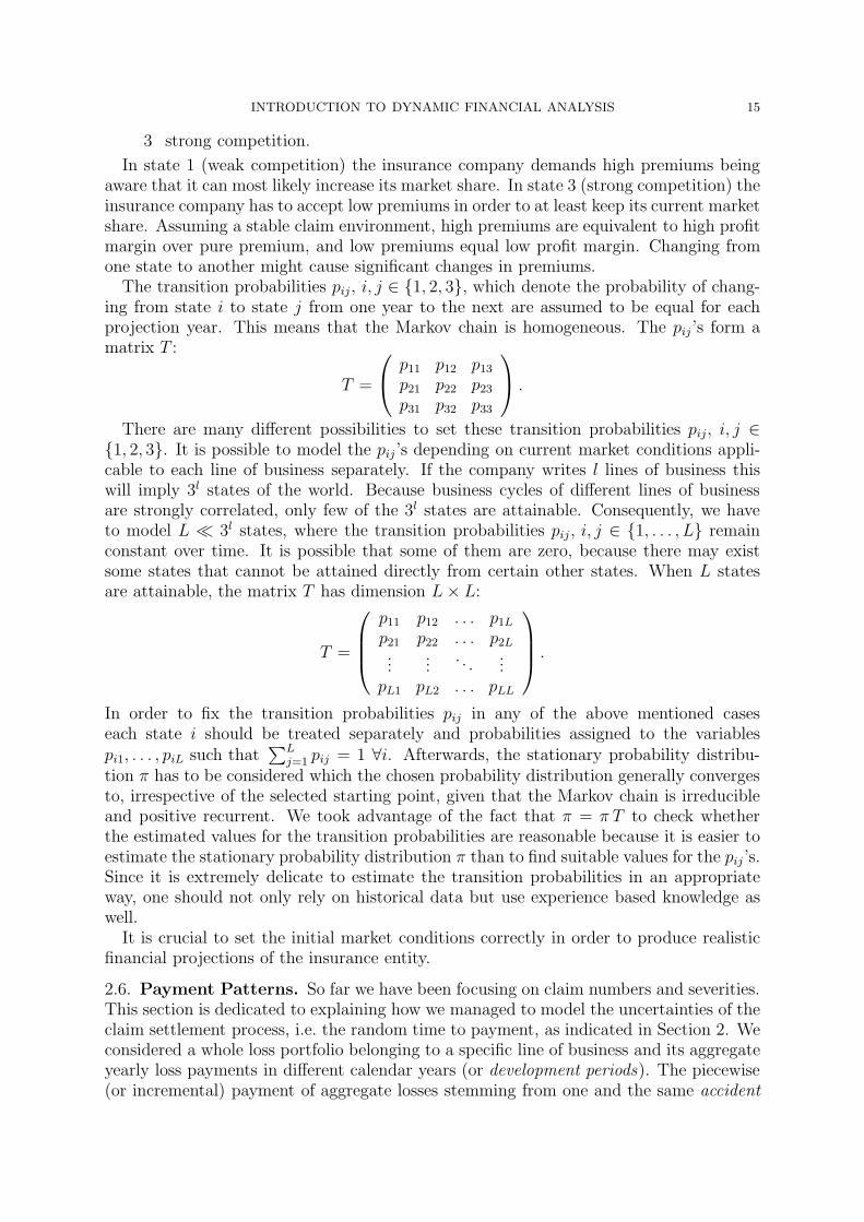
In state 1 (weak competition) the insurance company demands high premiums beingaware that it can most likely increase its market share. In state 3 (strong competition) theinsurance company has to accept low premiums in order to at least keep its current marketshare. Assuming a stable claim environment, high premiums are equivalent to high profitmargin over pure premium, and low premiums equal low profit margin. Changing fromone state to another might cause significant changes in premiums.The transition probabilities pij, i, j ∈ {1, 2, 3}, which denote the probability of chang-

ing from state i to state j from one year to the next are assumed to be equal for eachprojection year. This means that the Markov chain is homogeneous. The pij ’s form amatrix T :

T =

p11 p12 p13p21 p22 p23p31 p32 p33

.There are many different possibilities to set these transition probabilities pij, i, j ∈

{1, 2, 3}. It is possible to model the pij ’s depending on current market conditions appli-cable to each line of business separately. If the company writes l lines of business thiswill imply 3l states of the world. Because business cycles of different lines of businessare strongly correlated, only few of the 3l states are attainable. Consequently, we haveto model L � 3l states, where the transition probabilities pij , i, j ∈ {1, . . . , L} remainconstant over time. It is possible that some of them are zero, because there may existsome states that cannot be attained directly from certain other states. When L statesare attainable, the matrix T has dimension L× L:

T =

p11 p12 . . . p1L

p21 p22 . . . p2L...

.... . .

...pL1 pL2 . . . pLL

.In order to fix the transition probabilities pij in any of the above mentioned caseseach state i should be treated separately and probabilities assigned to the variablespi1, . . . , piL such that

∑Lj=1 pij = 1 ∀i. Afterwards, the stationary probability distribu-

tion π has to be considered which the chosen probability distribution generally convergesto, irrespective of the selected starting point, given that the Markov chain is irreducibleand positive recurrent. We took advantage of the fact that π = π T to check whetherthe estimated values for the transition probabilities are reasonable because it is easier toestimate the stationary probability distribution π than to find suitable values for the pij ’s.Since it is extremely delicate to estimate the transition probabilities in an appropriateway, one should not only rely on historical data but use experience based knowledge aswell.It is crucial to set the initial market conditions correctly in order to produce realistic

financial projections of the insurance entity.

2.6. Payment Patterns. So far we have been focusing on claim numbers and severities.This section is dedicated to explaining how we managed to model the uncertainties of theclaim settlement process, i.e. the random time to payment, as indicated in Section 2. Weconsidered a whole loss portfolio belonging to a specific line of business and its aggregateyearly loss payments in different calendar years (or development periods). The piecewise(or incremental) payment of aggregate losses stemming from one and the same accident


✲ developmentyear t2

❄accidentyear t1

t0−9

t0−8

t0−7

t0−6

t0−5

t0−4

t0−3

t0−2

t0−1

t0t0+1

t0+2

t0+3

t0+4

t0+5

0 1 2 3 4 5 6 7 8 9 10 11 12 13 14

�calendaryear t1+t2

Figure 2.1. Paid losses (upper left triangle), outstanding loss paymentsand future loss payments.

year forms a payment pattern. An (incremental) payment pattern is a vector with lengthequal to an assumed number of development periods. The i-th vector component describesthe percentage of estimated ultimate loss amount (on aggregate portfolio level) to be paidout in the (i−1)-st development year. If we consider yearly loss payments pertaining toa specific accident year t then the i-th development year refers to calendar year t+ i.In the following we will denote accident years by t1 and development years by t2. For

simplicity’s sake, we will drop the index representing line of business for the most partof this section.Very often one finds payment patterns treated as being deterministic in DFA models.

This will be justified by pointing out that payment patterns do not change significantlyfrom one year to the next. We believe that in order to account for reserving risk in aDFA model properly one has to have a stochastic model for the timing of loss paymentsas well.Generally, for each prior accident year considered, the loss amounts which have been

paid to date are known. Figure 2.1 displays this in graphical format. The triangleformed by the area on the left hand side of the bold line – the loss triangle – representsempirical, i.e. known, loss payments whereas the remaining parts represent outstandingand future loss payments, which are unknown. For example, if we assume to be at theend of calendar year 2000 (t0 = 2000) considering accident year 1996 (= t0 −4), we knowthe loss amounts pertaining to accident year 1996, which have been paid out in calendaryears 1996, 1997, . . . , 2000. But we do not know the amounts that will be paid in calendaryear 2001 and later. Some very popular actuarial techniques for estimating outstandingloss payments – which are characterized by those cell entries (t1, t2), t1 ≤ t0, belonging tothe right hand side of the bold line – are based on deriving an average payment patternfrom loss payments represented by the loss triangle.In the simplified model description of this section we will not take into account the

empirical fact that payment patterns of single large losses differ from those of aggregate


losses. We will also disregard changes in future claim inflation, although it might have astrong impact on certain lines of business.For each line we assumed an ultimate development year τ when all claims arising from

an accident year would be paid completely. Incremental claim payments denoted by Zt1,t2

are known for previous years t1 + t2 ≤ t0. Ultimate loss amounts Zultt1

:=∑τ

t=0 Zt1,t varyby accident year t1. In order to determine loss reserves taking into account reserving riskwe first had to simulate random loss payments Zt1,t2 . As a second step we needed to havea procedure for estimating ultimate loss amounts Zult

t1at each future time.

We distinguished two cases. First we will explain the modelling of outstanding losspayments pertaining to previous accident years followed by a description to model losspayments in respect of future accident years.For previous accident years (t1 ≤ t0) payments Zt1,t2 , with t1 + t2 ≤ t0 are known.

We used them as a basis for predicting outstanding payments. We used a chain-laddertype procedure (for the chain-ladder method, see Mack [31]), i.e. we applied ratios tocumulative payments per accident year. The following type of loss development factorwas defined

(2.23) dt1,t2 :=Zt1,t2∑t2−1t=0 Zt1,t

, t2 ≥ 1.

Note that this ratio is not a typical chain-ladder link ratio. When mentioning loss devel-opment factors in this section we are always referring to factors defined by (2.23).Since a lognormal distribution usually provides a good fit to historical loss development

factors, we used the following model for outstanding loss payments in calendar yearst1 + t2 ≥ t0 + 1 for accident years t1 ≤ t0:

(2.24) Zt1,t2 = dt1,t2 ·t2−1∑t=0

Zt1,t ,

where

dt1,t2 ∼ lognormal(µt2, σ2t2),

µt2 = estimated logarithmic loss development factor for

development year t2, based on historical data,

σt2 = estimated logarithmic standard deviation of loss

development factors, based on historical data.

This loss payment model is able to provide realistic loss payments as long as there havebeen no significant structural changes in the loss history. However, if for an accident yeart1 ≤ t0 a high percentage of ultimate claim amount had been paid out in one of the firstdevelopment years t2 ≤ t0 − t1, this approach would increase the reserve due to higherdevelopment factors leading to overestimation of outstanding payments. Consequently,single large losses should be treated separately. Sometimes changes in law affect insurancecompanies seriously. Such unpredictable structural changes are an important risk. A well-known example are health problems caused by buildings contaminated with asbestos.These were responsible for major losses in liability insurance. Such extreme cases shouldperhaps be modelled by separate scenarios.


Ultimate loss amounts for accident years t1 ≤ t0 were calculated as

(2.25) Zultt1

=τ∑

t=0

Zt1,t.

The second type of loss payments are due to future accident years t1 ≥ t0 + 1. Thecomponents determining total loss amounts in respect of these accident years have alreadybeen explained in Sections 2.3 and 2.4:

(2.26) Zultt1(k) =

2∑j=0

N jt1(k) X

jt1(k) + bt1(k)

Mt1∑i=1

Y kt1,i − Rt1(k) ,

where

N jt1(k) = number of non-catastrophe losses in accident year t1 for

line of business k and renewal class j, see (2.17),

Xjt1(k) = severity of non-catastrophe losses in accident year t1 for

line of business k and renewal class j, see (2.19),

bt1(k) = market share of the company in year t1 for line of business k,

Mt1 = number of catastrophes in accident year t1, see (2.20),

Y kt1,i = severity of catastrophe i in line of business k in accident

year t1, see (2.22),

Rt1(k) = reinsurance recoverables; a function of the Y kt1,i’s, depending

on the company’s reinsurance program.

It remains to model the incremental payments of these ultimate loss amounts over thedevelopment periods. Therefore, we simulated incremental percentages At1,t2 of ultimateloss amount by using a beta probability distribution with parameters based on paymentpatterns of previous calendar years:

(2.27) At1,t2 =

{Bt1,0 for t2 = 0,

Bt1,t2

(1−∑t2−1

t=0 At1,t

)for t2 ≥ 1,

where

Bt1,t2 = incremental loss payment due to accident year t1 in development

year t2 in relation to the sum of remaining incremental loss

payments pertaining to the same accident year

∼ beta(α, β), α, β > −1.

Here α and β are chosen to yield

mt1,t2 = E [Bt1,t2 ] =α + 1

α + β + 2,

vt1,t2 = Var (Bt1,t2) =(α + 1) (β + 1)

(α + β + 2)2 (α+ β + 3),

(2.28)


where

mt1,t2 = estimated mean value of incremental loss payment due to accident

year t1 in development year t2 in relation to the sum of remaining

incremental loss payments pertaining to the same accident year,

based onAt1−1,t2∑τt=t2

At1−1,t,

At1−2,t2∑τt=t2At1−2,t

, . . . ,

vt1,t2 = estimated variance, based on the same historical data.

It can happen that α>−1, β >−1 satisfying (2.28) do not exist. This means that theestimated variance reaches or exceeds the maximum variance mt1,t2(1−mt1,t2) possible fora beta distribution with mean mt1,t2 . In this case, we resorted to a Bernoulli distributionfor Bt1,t2 because the Bernoulli distribution marks a limiting case of the beta distribution:

Bt1,t2 ∼ Be(mt1,t2).

This approach limited the maximum variance to mt1,t2(1−mt1,t2).For each future accident year (t1 ≥ t0) we finally calculated loss payments in develop-

ment year t2 by:

(2.29) Zt1,t2 = At1,t2 Zultt1 .

So far we have been dealing with the simulation of incremental claim payments due toan accident year. We still have to explain how we arrived at reserve estimates at eachtime during the projection period. For each accident year t1 we estimated the ultimateclaim amount in each development year t2 through:

(2.30) Zultt1,t2 =

τ∏t=t2+1

(1 + eµt)

t2∑t=0

Zt1,t ,

where

µt = estimated logarithmic loss development factor for

development year t, based on historical data,

Zt1,t = simulated losses for accident year t1, to be paid in

development year t, see (2.24) and (2.29).

Note that (2.30) is an estimate at the end of calendar year t1+t2, whereas (2.26) representsthe real future value. Reserves in respect of accident year t1 at the end of calendar yeart1 + t2 are determined by the difference between estimated ultimate claim amount Zult

t1,t2and paid to date losses in respect of accident year t1. Reserving risk materializes throughvariations of the difference between the simulated (real) ultimate claim amounts and theestimated values.Similarly, at the end of calendar year t1+ t2 we got an estimate for discounted ultimate

losses for each accident year t1. Note that only future loss payments are discountedwhereas paid to date losses are taken at face value:

(2.31) Zult,disct1,t2 =

(1 + e−Rt1+t2,1eµt2+1 +

τ∑s=t2+2

e−Rt1+t2,s−t2eµs

s−1∏t=t2+1

(1 + eµt)

) t2∑t=0

Zt1,t ,


where

Rt,T = T year spot rate at time t, see (2.7),

µt = estimated logarithmic loss development factor for

development year t, based on historical data,

Zt1,t = simulated losses for accident year t1, paid in

development year t, see (2.24) and (2.29).

Interesting references on stochastic models in loss reserving are Christofides [8] andTaylor [40].

3. The Corporate Model: From Simulations to Financial Statements

As pointed out in Section 1.4, DFA is an approach to facilitate and help justify manage-ment decisions. These are driven by a variety of considerations: maximizing shareholdervalue, constraints imposed by regulators, tax optimization and rankings by rating agenciesand analysts. Parties outside the company rely on financial reports in making decisionsregarding their relationship with the company. Therefore, a DFA model has to bridgethe gap between stochastic simulation of cash flows and financial statements (pro formabalance sheets and income statements). The accounting process helps organize cash flowsimulations into a readily understood and consistent financial structure. This requiresa substantial number of accrual items to be generated in order to develop accountingentries for the model’s financial statements.A DFA model has to allow for a statutory accounting framework if it wants to address

solvency requirements imposed by regulators thoroughly. If the focus is on shareholdervalue the model should predominantly be concerned with economic values, implying, forexample, assets being marked-to-market and all policy liabilities being discounted. Whilestatutory accounting focuses on solvency and balance sheet, generally accepted accountingprinciples (GAAP) emphasize income statements and comparability between entities ofdifferent nature. Consequently, a perfect DFA model should, among other things, includedifferent accounting frameworks (i.e. statutory, GAAP and economic). This increasesimplementation costs substantially. A less burdensome approach would be to concentrateon GAAP accounting taking into account solvency requirements by introducing them asconstraints to the model where appropriate. Our DFA implementation focused on aneconomic perspective.In order to keep the exposition simple and within reasonable size we will mention only

some key relationships of the corporate model. A much more comprehensive descriptionis given in Kaufmann [24].One of the fundamental variables is (economic) surplus Ut, defined as the difference be-

tween the market value of assets and the market value of liabilities (derived by discountingloss reserves and unearned premium reserves). The amount of available surplus reflectsthe financial strength of an insurance company and serves as a measure for shareholdervalue. We consider a company as being insolvent once Ut < 0.Change in surplus is determined by the following cash flows:

(3.1) ∆Ut = Pt + (It − It−1) + (Ct − Ct−1)− Zt − Et − (Rt − Rt−1)− Tt,


where

Pt = earned premiums,

It = market value of assets (including realized capital gains in year t),

Ct = equity capital,

Zt = losses paid in calendar year t,

Et = expenses,

Rt = (discounted) loss reserves,

Tt = taxes.

Note that Ct − Ct−1 describes the result of capital measures like issuance of new equitycapital or capital reduction.We derived earned from written premiums. For each line of business, written premiums

P jt for renewal class j should depend on change in loss trends, the position in the under-

writing cycle and on the number of written exposures. This leads to written premium P jt

of

(3.2) P jt = (1 + δP

t ) (1 + cmt−1,mt)wj

t

wjt−1

P jt−1 , j = 0, 1, 2 ,

where

δPt = change in loss trends, see remarks after (2.11),

mt = market condition in year t, see Section 2.5,

cA,B = constant that describes how premiums develop when

changing from market condition A to B; cA,B can be

estimated based on historical data,

w0t = written exposure units for new business,

w1t = written exposure units for renewal business, first renewal,

w2t = written exposure units for renewal business, second and

subsequent renewals.

Description of the calculation of initial values P jt0 in (3.2) will be deferred to the paragraph

subsequent to equation (3.4). Variables cA,B have to be available as input parametersat the start of the DFA analysis. When estimating the percentage change of premiumsimplied by changing from market condition A to B it seems plausible to assume that thefinal impact is zero if market conditions change back from B to A. This translates into(1+cA,B)(1+cB,A) = 1. Also, the impact on premium changes triggered by changing frommarket condition A to B and from B to C afterwards should be the same as changingfrom A to C directly: (1 + cA,B)(1 + cB,C) = (1 + cA,C). We assumed an autoregressiveprocess of order 1, AR(1), for the modelling of exposure unit development:

(3.3) wjt = (aj + bj wj

t−1 + εjt )

+, j = 0, 1, 2 ,

where

εjt ∼ N (0, (σj)2), εj1, εj2, . . . i.i.d.,

aj , bj , σj = parameters that can be estimated based on historical data.


The initial values wjt0 are known since they represent the current number of exposure

units. Choosing parameter bj < 1 ensures stationarity of the AR(1) process (3.3). Whenderiving parameters aj and bj , prior adjustments to historical data might be necessaryif jumps in number of exposure units had occurred caused by acquisition or transfer ofloss portfolios. We found it helpful to admit deterministic modelling of exposure growthas well in order to allow for these effects, which are mostly anticipated before changes inthe composition of the portfolio become effective.Setting premium rates based on knowledge of past loss experience and exposure growth

as expressed in (3.2) leaves us still with substantial uncertainties with regard to the ade-quacy of premiums. These uncertainties are conveyed in the term underwriting risk. Notethat written premiums represented by equation (3.2) would come close to be adequate

if the realizations of all random variables referring to projection year t (δPt , cmt−1,mt , w

jt )

were known in advance and assuming adequacy of current premiums P jt0 . Unfortunately,

premiums to be charged in year t have to be determined prior to the beginning of year t.Therefore, random variables in (3.2) have to be replaced by estimations in order to modelwritten premiums P j

t , which would be charged in projection year t.

(3.4) P jt = (1 + δP

t ) (1 + cmt−1,mt)wj

t

wjt−1

P jt−1 , j = 0, 1, 2 ,

where we got the estimates via their expected values:

δPt = [1+ aX+bX(aI+bI(ab+(1−a)rt−1))][1+a

F+bF (aI+bI(ab+(1−a)rt−1))]−1,

see (2.11), (2.10), (2.9), (2.8) and (2.4).

cmt−1,mt =

l(k)∑m=1

pmt−1,m cmt−1,m ,

l(k) = number of states for line of business k, see Section 2.5,

pmt−1,m = transition probability, see Section 2.5.

wjt = a

j + bj wjt−1, see (3.3).

While (3.2) represents a random variable that describes (almost) adequate premiums,(3.4) is the expected value of this random variable representing actually written premiums.Note that the time index t = t0 refers to the year prior to the first projection year. Bycombining (3.2) and (3.4) we deduce that the initial values P j

t0 can be calculated via P jt0 :

(3.5) P jt0 =

1 + δPt0

1 + δPt0

1 + cmt0−1,mt0

1 + cmt0−1,mt0

wjt0

wjt0

P jt0 , j = 0, 1, 2 .

P jt0 represent written premiums charged for the last year and still valid just before the

start of the first projection year. We assumed that premiums P jt0 were adequate and

based on established premium principles allowing for the cost of capital to be earned.An alternative of setting starting values according to (3.5) would be to use business plandata instead. This is an approach applicable at several places of the model.By using written premiums P j

t (k) as given in (3.4) where the index k denotes lineof business, we got the following expression for total earned premiums of all lines and


renewal classes (see explanation in Section 2.3) combined:

(3.6) Pt =

l∑k=1

2∑j=0

ajt (k)P

jt (k) +

(1− aj

t−1(k))P j

t−1(k) ,

where

ajt (k) = percentage of premiums earned in year written,

estimated based on historical data.

We restricted ourselves to modelling only the most important asset classes, i.e. fixedincome type investments (e.g. bonds, policy loans, cash), stocks, and real estate. Mod-elling of stock returns has already been mentioned in Section 2.2, future prices of fixedincome investments can be derived from the generated term structure explained in Sec-tion 2.1. Our approach of modelling real estate was very similar to the stock return modelof Section 2.2.Future investment profits depend not only on the development of market values of assets

currently on the balance sheet but also on decisions how new funds will be reinvested.In order to build a DFA model that really deserves to be called dynamic we shouldaccount for potential changes of asset allocation in future years compared to a pure staticapproach that keeps the asset allocation unchanged. This requires defining investmentrules depending on specific economic conditions.Capital measures ∆Ct = Ct − Ct−1 were modelled as additions or deductions from

surplus depending on a target reserves-to-surplus ratio. A purely deterministic approachthat increased or decreased equity capital by a certain amount at specific times wouldhave been an alternative.Aggregate loss payments in projection year t were calculated based on variables defined

in Section 2.6:

(3.7) Zt =l∑

k=1

τ(k)∑t2=0

Zt−t2,t2(k),

where

Zt−t2,t2(k) = losses for accident year t− t2, paid in development

year t2; see (2.24) and (2.29),

τ(k) = ultimate development year for this line of business,

k = line of business.

We used a simple approach for modelling general expenses Et. They were calculatedas a constant plus a multiple of written exposure units wj

t (k). The appropriate interceptaE(k) and slope bE(k) were determined by linear regression:

(3.8) Et =

l∑k=1

(aE(k) + bE(k)

2∑j=0

wjt (k)

).

For loss reserves Rt we got

(3.9) Rt =l∑

k=1

τ(k)∑t2=0

(Zult,disc

t−t2,t2 (k)−t2∑

s=0

Zt−t2,s(k)

),


interest rates

inflation

stock returns

loss severity loss frequency

investment returns

losses

exposure units

premiums expenses

surplus

stochastic

deterministic

Figure 4.1. Schematic description of the modelling process: stochasticand deterministic influences on surplus.

where

Zult,disct−t2,t2 (k) = estimation in calendar year t for discounted ultimate

losses in accident year t− t2; see (2.31),Zt−t2,s(k) = losses for accident year t− t2, paid in development

year s; see (2.24) and (2.29),

τ(k) = ultimate development year,

k = line of business.

An important variable to be considered are taxes, Tt, because many management deci-sions are tax driven. The proper treatment of taxes depends on the accounting framework.We used a rather simple tax model allowing for current income taxes only, i.e. neglectingthe possibility of deferred income taxes for GAAP accounting.

4. DFA in Action

The aim of this section is to give an example of potential applications of DFA. Figure 4.1displays the model logic of the approach introduced in this paper in graphical format. Byproviding a simple example we will show how to analyze surplus and ruin probabilities.It was not intended to describe a specific effect when using the parameters given below.The parameters were made up, i.e. they were not based on a real case.

Simplifying assumptions

• Only one line of business.


• New business and renewal business are not modelled separately.• Payment patterns are assumed to be deterministic.• No transaction costs.• No taxes.• No dividends paid.

Model choices

• Number of non-catastrophe losses ∼ NB (154, 0.025).• Mean severity of non-catastrophe losses ∼ Gamma (9.091, 242), inflation-adjusted.• Number of catastrophes ∼ Pois (18).• Severity of individual catastrophes ∼ lognormal (13, 1.52), inflation-adjusted.• Optional excess of loss reinsurance with deductible 500 000 (inflation-adjusted),and cover ∞.

• Underwriting cycles: 1 = weak, 2 = average, 3 = strong. State in year 0:1 (weak). Transition probabilities: p11 = 60%, p12 = 25%, p13 = 15%,p21 = 25%, p22 = 55%, p23 = 20%, p31 = 10%, p32 = 25%, p33 = 65%.

• All liquidity is reinvested. There are only two investment possibilities:1) buy a risk-free bond with maturity one year,2) buy an equity portfolio with a fixed beta.

• Market valuation: assets and liabilities are stated at market value, i.e. assets arestated at their current market values, liabilities are discounted at the appropriateterm spot rate determined by the model.

Model parameters

• Interest rates, see (2.4): a = 0.25, b = 5%, s = 0.1, r1 = 2%.• General inflation, see (2.8): aI = 0%, bI = 0.75, σI = 0.025.• No inflation impacting the number of claims.• Inflation impacting severity of claims, see (2.10):aX = 3.5%, bX = 0.5, σX = 0.02.

• Stock returns, see (2.14), (2.15) and (2.15):aM = 4%, bM = 0.5, βS

t ≡ 0.5, σ = 0.15.• Market share: 5%.• Expenses: 28.5% of written premiums.• Premiums for reinsurance: 175 000 p.a. (inflation-adjusted).

Historical data

• Written premiums in the last year: 20 million.• Initial surplus: 12 million.

Strategies considered

• Should the company buy reinsurance coverage or not?• How should the reinvestment of excess liquidity be split between fixed incomeinstruments and stocks?

Projection period

• 10 years (yearly intervals).

Risk and return measures

• Return measure: expected surplus E[U10].• Risk measure: ruin probability, defined as P[U10 < 0].


a b

with withoutreinsurance reinsurance

1 100% bonds 23.17mio. 23.29mio.0% stocks 0.49% 1.15%



4 ≤ 5mio. bonds 26.48mio. 26.79mio.rest stocks 6.08% 6.52%

5 ≤10mio. bonds 25.74mio. 26.06mio.rest stocks 3.64% 4.49%

6 ≤20mio. bonds 24.62mio. 24.95mio.rest stocks 0.90% 1.65%

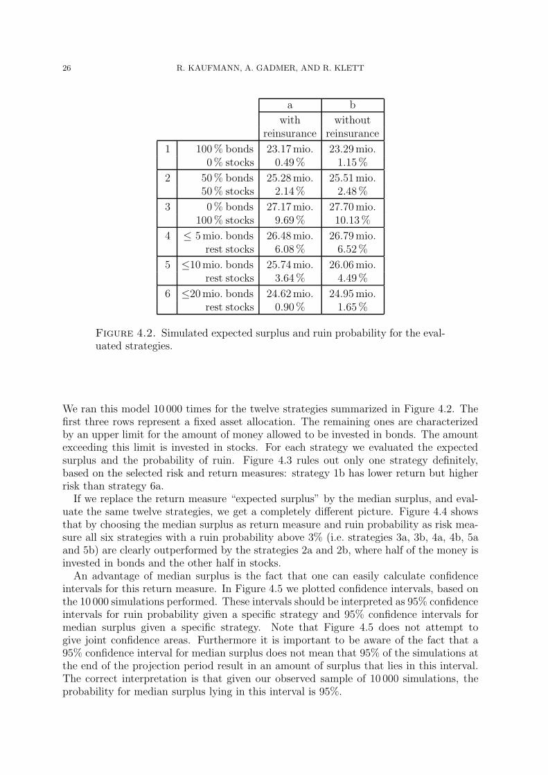
Figure 4.2. Simulated expected surplus and ruin probability for the eval-uated strategies.

We ran this model 10 000 times for the twelve strategies summarized in Figure 4.2. Thefirst three rows represent a fixed asset allocation. The remaining ones are characterizedby an upper limit for the amount of money allowed to be invested in bonds. The amountexceeding this limit is invested in stocks. For each strategy we evaluated the expectedsurplus and the probability of ruin. Figure 4.3 rules out only one strategy definitely,based on the selected risk and return measures: strategy 1b has lower return but higherrisk than strategy 6a.If we replace the return measure “expected surplus” by the median surplus, and eval-

uate the same twelve strategies, we get a completely different picture. Figure 4.4 showsthat by choosing the median surplus as return measure and ruin probability as risk mea-sure all six strategies with a ruin probability above 3% (i.e. strategies 3a, 3b, 4a, 4b, 5aand 5b) are clearly outperformed by the strategies 2a and 2b, where half of the money isinvested in bonds and the other half in stocks.An advantage of median surplus is the fact that one can easily calculate confidence

intervals for this return measure. In Figure 4.5 we plotted confidence intervals, based onthe 10 000 simulations performed. These intervals should be interpreted as 95% confidenceintervals for ruin probability given a specific strategy and 95% confidence intervals formedian surplus given a specific strategy. Note that Figure 4.5 does not attempt togive joint confidence areas. Furthermore it is important to be aware of the fact that a95% confidence interval for median surplus does not mean that 95% of the simulations atthe end of the projection period result in an amount of surplus that lies in this interval.The correct interpretation is that given our observed sample of 10 000 simulations, theprobability for median surplus lying in this interval is 95%.


••

•

•

•

•

•

•

•

•

•

•

ruin probability (%)

expe

cted

sur

plus

(m

illio

ns)

0 2 4 6 8 10

2425

2627

1a 1b

2a

2b

3a

3b

4a

4b

5a

5b

6a

6b

Figure 4.3. Graphical comparison of ruin probabilities and expected sur-plus for selected business strategies.

•

•

•

•

•

•

•

•

•

•

•

•


med

ian

surp

lus

(mill

ions

)

0 2 4 6 8 10

21.5

22.0

22.5

23.0

23.5

24.0

1a

1b

2a

2b

3a

3b

4a

4b

5a

5b

6a

6b

Figure 4.4. Graphical comparison of ruin probabilities and median sur-plus for selected business strategies.



med

ian

surp

lus

(mill

ions

)

0 2 4 6 8 10

21.5

22.0

22.5

23.0

23.5

24.0

Figure 4.5. 95% confidence intervals for ruin probability and median sur-plus, based on 10 000 simulations for each strategy.

5. Some Remarks on DFA

5.1. Discussion Points. This introductory paper discussed only the most relevant issuesrelated to DFA modelling. Therefore, we would like to mention briefly some additionalpoints without necessarily being exhaustive.

5.1.1. Deterministic Scenario Testing. In Section 1 we mentioned the superiority of DFAcompared to deterministic scenario testing. This does not imply that the latter methodis useless at all. On the contrary, deterministic scenario testing is a very useful thing, inparticular when it comes to assess the impact of extreme events at pre-defined dates orwhen specific macroeconomic influences are to be evaluated. It is a very useful feature ofa DFA tool being able to switch off stochasticity and return to deterministic scenarios.

5.1.2. Macroeconomic Environment. In life insurance financial modelling interest ratesare often considered to be the only macroeconomic factor affecting the values of assetsand liabilities. Hodes, Feldblum and Neghaiwi [21] have pointed out that in nonlifeinsurance, interest rates are only one of various other factors affecting liability values.In Worker’s Compensation in the US, for instance, unemployment rates and industrialcapacity utilization have greater effects on loss costs than interest rates have, while third-party motor claims are correlated with total volume of traffic and with sales of new cars.Although rarely done it might be worthwhile modelling specific macroeconomic driverslike industrial capacity utilization or traffic volume separately. This would require aforegoing econometric analysis of the dynamics of particular factors.


5.1.3. Correlations. DFA is able to allow for dependencies between different stochasticvariables. Before starting to implement these dependencies one should have a soundunderstanding of existing dependencies within an insurance enterprise. Estimating cor-relations from historical (loss) data is often not feasible due to aggregate figures andstructural changes in the past, e.g. varying deductibles, changing policy conditions, acqui-sitions, spin-offs, etc. Furthermore, recent research, see for example Embrechts, McNeiland Straumann [17] and [18], and Lindskog [28], suggests that linear correlation is notappropriate to model dependencies between heavy-tailed and skewed risks.We suggest modelling dependencies implicitly, as a result of a number of contributory

influences, for example, catastrophes that impact more than one line of business or interestrate changes affecting only specific lines. The majority of these relations should beimplemented based on economic and actuarial wisdom, see for instance Kreps [26].

5.1.4. Separate Modelling of New and Renewal Business. In the model outlined in thispaper we allowed for separate modelling of new and renewal business, see Section 2.3.Hodes, Feldblum and Neghaiwi [21] pointed out that this makes perfectly sense due todifferent stochastic behavior of the respective loss portfolios. Furthermore, having thissplit allows a deeper analysis of value drivers within the portfolio and marks an importantstep towards determining an appraised value for a nonlife insurance company.

5.1.5. Model Validation. What is finally a good DFA model and what is not? Experience,knowledge and intuition of users from actuarial, economic and management side play adominant role in evaluating a DFA model. A danger in this respect might be that non-intuitive results could be blamed on a bad model instead of wrong assumptions. A furtherpossibility to evaluate a model is to test results coming out of the DFA model againstempirical results. This will only be feasible in very few restricted cases because it wouldrequire keeping track of data for several years. However, model validation should deservemore attention. This needs to be recommended in particular to those practitioners dealingwith software vendors of DFA tools who do not intend to justify their decision of buyingan expensive DFA product by referring to the software design only.

5.1.6. Model Calibration. We have already touched on this at several places and pointedto its importance within a DFA analysis. However sophisticated a DFA tool or modelmight be, it has to be fed with data and parameter values. Studies have shown that themajor part of a DFA analysis had been devoted to this exercise. Usually, the calibrationpart is an ongoing process during the course of an analysis in order to fine-tune the model.

5.1.7. Interpretation of Output. We mentioned in Section 1.5 that the interpretation pro-cess of DFA output follows very often traditional patterns, e.g. efficient frontier analysis,which might lead to false or at least questionable conclusions, see Cumberworth, Hitch-cox, McConnell and Smith [10]. Another example showing how critical interpretationof results can be is this: A net present value (NPV) analysis applied to model officecash flows can generate or destroy a huge amount of shareholder value by making slightchanges to CAPM assumptions, which are often used for determining the discount rate.A way to keep feet on sound economic ground and simultaneously remove a great deal ofarbitrariness is through resorting to deflators, see Jarvis, Southall and Varnell [23]. Theuse of this concept, originating in the work of Arrow and Debreu, has been promoted bySmith [39] and is further discussed in Buhlmann, Delbaen, Embrechts and Shiryaev [7].


The cited references might be evidence for growing awareness that our toolbox for inter-preting and understanding DFA results needs to be renovated in order to enhance theuse of DFA.

5.2. Strength and Weaknesses of DFA. DFA models provide generally deeper in-sight into risks and potential rewards of business strategies than scenario testing cando. DFA marks a milestone towards evaluating business strategies when compared toold-style analysis of considering only key ratios. DFA is virtually the only feasible way tomodel an entire nonlife operation on a cash flow basis. It allows for a high degree of detailincluding analysis of the reinsurance program, modelling of catastrophic events, depen-dencies between random elements, etc. DFA can meet different objectives and addressdifferent management units (underwriting, investments, planning, actuarial, etc.).Nevertheless, it is worth mentioning that a DFA model will never be able to capture

the complexity of the real-life business environment. Necessarily, one has to restrictattention during the model building process to certain features the model is supposed toreflect. However, the number of parameters which have to be estimated beforehand andthe number of random variables to be modelled even within medium-sized DFA modelscontribute a big deal of process and parameter risk to a DFA model. Furthermore one hasto be aware that results will strongly depend on the assumptions used in the model set-up.A critical question is: How big and sophisticated should a DFA model be? Everythingcomes at a price and a simple model that can produce reasonable results will probablybe preferred by many users due to growing reluctance of using non-transparent “blackboxes”. In addition, smaller models tend to be more in line with intuition, and makeit easier to assess the impact of specific variables. A good understanding and control ofuncertainties and approximations is vital to the usefulness of a DFA model.

5.3. Closing Remarks. We wanted to give an introduction into DFA by hinting to pit-falls and emphasizing important issues to be taken into account in the modelling process.Our intention was to provide the uninformed reader with a simple DFA approach enablingthese readers to implement DFA using our approach as a kind of reference model. Manycommercial DFA tools are roughly structured as the model outlined in this paper. Spe-cific concepts and concrete implementation of the model components are often different.We are absolutely aware that there are numerous alternatives to each of the sub-modelsintroduced in this paper. Some of them might be much more powerful or flexible thanour approach. We wanted to provide a framework leaving it up to the reader to completethe DFA house by making adjustments or amendments at his/her discretion. Althoughwe did not necessarily target the DFA experts our exposition might have also served togive an impression of the complexity of a fully fledged DFA model.

Acknowledgement. We would like to thank Paul Embrechts, Peter Blum and theanonymous referees for numerous comments on an earlier version of the paper. Wealso benefited substantially from discussions on DFA with Allan Kaufman and StavrosChristofides.

References

[1] Ahlgrim K.C., D’Arcy S.P. and Gorvett R.W. (1999) Parametrizing Interest Rate Models, CasualtyActuarial Society Forum, 1–50.

[2] Artzner P., Delbaen F., Eber J. and Heath D. (1997) Thinking Coherently, RISK 10, 68–71.


[3] Artzner P., Delbaen F., Eber J. and Heath D. (1999) Coherent Measures of Risk, MathematicalFinance 9, no. 3, 203–228.

[4] Bjork T. (1996) Interest Rate Theory. In Financial Mathematics (ed. W. Runggaldier), LectureNotes in Mathematics 1656, 53–122, Springer, Berlin.

[5] Blum P., Dacorogna M., Embrechts P., Neghaiwi T. and Niggli H. (2001) Using DFA for Modellingthe Impact of Foreign Exchange Risks on Reinsurance Decisions, Paper presented at the CasualtyActuarial Society 2001 Reinsurance Meeting on Using Dynamic Financial Analysis to OptimizeCeded Reinsurance Programs and Retained Portfolios, Washington D.C., July 2001. Available asETH Zurich preprint.

[6] Brennan M.J. and Schwartz E.S. (1982) An Equilibrium Model of Bond Pricing and a Test of MarketEfficiency, Journal of Financial and Quantitative Analysis 17, 301–329.

[7] Buhlmann H., Delbaen F., Embrechts P. and Shiryaev A.N. (1998) On Esscher Transforms in Dis-crete Finance Models, ASTIN Bulletin 28(2), 171–186.

[8] Christofides S. (1990) Regression Models Based on Log-Incremental Payments, Claims ReservingManual 2, Institute of Actuaries, London.

[9] Cox J.C., Ingersoll J.E. and Ross S.A. (1985) A Theory of the Term Structure of Interest Rates,Econometrica 53, 385–407.

[10] Cumberworth M.P., Hitchcox A.M., McConnell W.M. and Smith A.D. (1999) Corporate Deci-sions in General Insurance: Beyond the Frontier, available from http://www.actuaries.org.uk/library/sessional meeting papers.html.

[11] D’Arcy S.P. and Doherty N. (1989) The Aging Phenomenon and Insurance Prices, Proceedings ofthe Casualty Actuarial Society 76, 24–44.

[12] D’Arcy S.P. and Doherty N. (1990) Adverse Selection, Private Information and Lowballing in In-surance Markets, Journal of Business 63, 145–164.

[13] D’Arcy S.P., Gorvett R.W., Herbers J.A., Hettinger T.E., Lehmann S.G. and Miller M.J. (1997)Building a Public Access PC-Based DFA Model, Casualty Actuarial Society Forum, 1–40.

[14] D’Arcy S.P., Gorvett R.W., Hettinger T.E. and Walling R.J. (1998) Using the Public Access DFAModel: A Case Study, Casualty Actuarial Society Forum, 55–118.

[15] Daykin C.D., Pentikainen T. and Pesonen M. (1994) Practical Risk Theory for Actuaries, Chapman& Hall, London.

[16] Embrechts P., Kluppelberg C. and Mikosch T. (1997) Modelling Extremal Events for Insurance andFinance, Springer, Berlin.

[17] Embrechts P., McNeil A.J. and Straumann D. (1999) Correlation: Pitfalls and Alternatives, RISK12(5), 69–71.

[18] Embrechts P., McNeil A.J. and Straumann D. (1999) Correlation and Dependence in Risk Man-agement: Properties and Pitfalls, Preprint ETH Zurich, available from http://www.math.ethz.ch/∼embrechts.

[19] Feldblum S. (1996) Personal Automobile Premiums: An Asset Share Pricing Approach for Prop-erty/Casualty Insurance, Proceedings of the Casualty Actuarial Society 83, 190–296.

[20] Heath D., Jarrow R. and Morton A. (1992) Bond Pricing and the Term Structure of Interest Rates:A New Methodology for Contingent Claim Valuation, Econometrica 60, 77–105.

[21] Hodes D.M, Feldblum S. and Neghaiwi A.A. (1999) The Financial Modeling of Property-CasualtyInsurance Companies, North American Actuarial Journal 3, no. 3, 41–69.

[22] Ingersoll J.E. (1987) Theory of Financial Decision Making, Rowman & Littlefield Studies in Finan-cial Economics, New Jersey.

[23] Jarvis S., Southall F.E. and Varnell E. (2001) Modern Valuation Techniques, Staple Inn ActuarialSociety, available from http://www.sias.org.uk/progold.htm.

[24] Kaufmann R. (1999) DFA: Stochastische Simulation zur Beurteilung von Unternehmensstrategienbei Nichtleben-Versicherungen, Master Thesis, ETH Zurich.

[25] Klett R. (1994) Asset-Liability-Management im Lebensversicherungsbereich, Master Thesis, Univer-sity of Freiburg.

[26] Kreps R.E. (2000) A Partially Comonotonic Algorithm for Loss Generation, Proceedings of XXXIstInternational ASTIN Colloquium, 165–176, Porto Cervo, Italy.

[27] Lamberton D. and Lapeyre B. (1996) Introduction to Stochastic Calculus Applied to Finance, Chap-man & Hall, London.


[28] Lindskog F. (2000) Modelling Dependence with Copulas and Applications to Risk Management,Master Thesis, ETH Zurich.

[29] Longstaff F.A. and Schwartz E.S. (1992) Interest Rate Volatility and the Term Structure: A Two-Factor General Equilibrium Model, Journal of Finance 47, 1259–1282.

[30] Lowe S.P. and Stanard J.N. (1997) An Integrated Dynamic Financial Analysis and Decision SupportSystem for a Property Catastrophe Reinsurer, ASTIN Bulletin 27(2), 339–371.

[31] Mack T. (1997) Schadenversicherungsmathematik, Verlag Versicherungswirtschaft E.V., Karlsruhe.[32] Markowitz H.M. (1959) Portfolio Selection: Efficient Diversification of Investments, John Wiley,

New York.[33] McNeil A.J. (1997) Estimating the Tails of Loss Severity Distributions using Extreme Value Theory,

ASTIN Bulletin 27(1), 117–137.[34] Modigliani M. and Miller M. (1958) The Cost of Capital, Corporation Finance, and the Theory of

Investment, American Economic Review 48, 261–297.[35] Musiela M. and Rutkowski M. (1998) Martingale Methods in Financial Modelling, 2nd edition,

Springer, Berlin.[36] Rogers L.C.G. (1995) Which Model for Term-Structure of Interest Rates Should One Use? In

Mathematical Finance, IMA Volume 65, 93–116, Springer, New York.[37] Schnieper R. (1997) Capital Allocation and Solvency Testing, SCOR Notes, 55–104.[38] Schnieper R. (1999) Solvency Testing, Mitteilungen der Schweizerischen Aktuarvereinigung, 11–45.[39] Smith A.D. (1996) How Actuaries Can Use Financial Economics, British Actuarial Journal 2(V),

1057–1193.[40] Taylor G.C. (2000) Loss Reserving: An Actuarial Perspective, Kluwer Academic Publishers, Boston.[41] Walling R.J., Hettinger T.E., Emma C.C. and Ackerman S. (1999) Customizing the Public Access

Model Using Publicly Available Data, Casualty Actuarial Society Forum, 239–266.[42] Wilkie A.D. (1995) More on a Stochastic Asset Model for Actuarial Use, British Actuarial Journal

1(V), 777–964.[43] Wise A.J. (1984) The Matching of Assets to Liabilities, Journal of the Institute of Actuaries 111,

445–485.[44] Woll R.G. (1987) Insurance Profits: Keeping Score, Financial Analysis of Insurance Companies,

Casualty Actuarial Society Discussion Paper Program, 446–533.

(R. Kaufmann) RiskLab, Department of Mathematics, ETH Zentrum, CH–8092 Zurich,

Switzerland

E-mail address: [email protected]

(A. Gadmer) Zurich Kosmos Versicherungen, Schwarzenbergplatz 15, A–1015 Wien, Aus-

tria


(R. Klett) Zurich Financial Services, Mythenquai 2, CH–8022 Zurich, Switzerland


Documents

What is DFA - RiskNET