What If Analysis Minggu 13. What-if analysis in Microsoft Excel What If Analysis, Slide 2Copyright © 2004, Jim Schwab, University of Texas at Austin What-if

What If Analysis

Minggu 13

What-if analysis in Microsoft Excel

What If Analysis, Slide 2 Copyright © 2004, Jim Schwab, University of Texas at Austin

What-if analysis is a powerful strategy for understanding the relationships in a data set and using this understanding to improve decision making. In order for what-if analysis to work, the relationships between the entities in a workbook should be linked by formulas instead of filled in with actual amounts. Using formulas enables the workbook to recalculate when we change an entry in one of the relationships. We will demonstrate what-if analysis using a multi-worksheet budget for Brunswick, Maine which I found on the Internet.

The Brunswick, Maine budget workbook contains a Summary worksheet and 29 detail worksheets, which provide details for each of the revenue and expenditure categories. The budget contains three versions: the first developed by the administrative departments in the city government, the second budget was presented by the city manager, and the third was the budget adopted by the city council. While all three budgets are similar, we do find areas where the city council cut expenditures from the departmental proposal , e.g. see the Public Works and Human Services detail worksheets.

Open the budget database


We will use an old budget from Brunswick, Maine to demonstrate doing what-if analysis in Excel.

We will use an old budget from Brunswick, Maine to demonstrate doing what-if analysis in Excel.

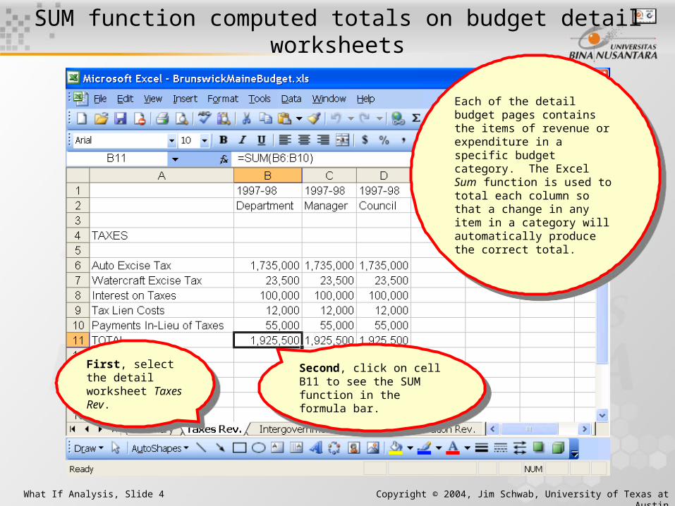
SUM function computed totals on budget detail worksheets


Each of the detail budget pages contains the items of revenue or expenditure in a specific budget category. The Excel Sum function is used to total each column so that a change in any item in a category will automatically produce the correct total.

Each of the detail budget pages contains the items of revenue or expenditure in a specific budget category. The Excel Sum function is used to total each column so that a change in any item in a category will automatically produce the correct total.

First, select the detail worksheet Taxes Rev.

First, select the detail worksheet Taxes Rev.

Second, click on cell B11 to see the SUM function in the formula bar.

Second, click on cell B11 to see the SUM function in the formula bar.

Displaying the formulas on the summary page - 1


In order to do what–if analysis, the various items on the worksheets must be connected by formulas so that a change in one item produces a change in the all the other items linked to the first item. If the worksheet cells contain the only numbers, a change in one item will not have an impact on the others.

In order to do what–if analysis, the various items on the worksheets must be connected by formulas so that a change in one item produces a change in the all the other items linked to the first item. If the worksheet cells contain the only numbers, a change in one item will not have an impact on the others.

First, select the summary worksheet Summary.

First, select the summary worksheet Summary.

Second, to see the formulas on the summary worksheet, select the Options command from the Tools menu.

Second, to see the formulas on the summary worksheet, select the Options command from the Tools menu.

Displaying the formulas on the summary page - 2


Next, click on the View tab in the Options dialog box to bring this page to the fore.

Next, click on the View tab in the Options dialog box to bring this page to the fore.

Finally, mark the Formulas checkbox and click on the OK button.

Finally, mark the Formulas checkbox and click on the OK button.

The formulas on the budget summary worksheet


Every cell in the Summary worksheet contains a formula, function, or reference to another cell in the workbook, except for the cells Taxable Valuation in the tax calculation section of the worksheet which are not contained any other place in the workbook.

Every cell in the Summary worksheet contains a formula, function, or reference to another cell in the workbook, except for the cells Taxable Valuation in the tax calculation section of the worksheet which are not contained any other place in the workbook.

For example, cell B6 on the Summary worksheet contains a reference to the cell on the detail worksheet that contains the sum function totaling the different tax items

For example, cell B6 on the Summary worksheet contains a reference to the cell on the detail worksheet that contains the sum function totaling the different tax items

Removing the display of formulas from the worksheet


To change the cell contents back so that they display numeric and text entries, we clear the check box for Formulas in the Options dialog.

To change the cell contents back so that they display numeric and text entries, we clear the check box for Formulas in the Options dialog.

After selecting the Options command from the Tools menu, clear the Formulas checkbox and click on the OK button.

After selecting the Options command from the Tools menu, clear the Formulas checkbox and click on the OK button.

Split worksheet so multiple parts can be viewed


First, scroll down the worksheet until row 21 is the top row in the window.

First, scroll down the worksheet until row 21 is the top row in the window.

Second, select row 29 as the row below where we want to locate the split.

Second, select row 29 as the row below where we want to locate the split.

Third, select the Split command from the Window menu.

Third, select the Split command from the Window menu.

'Total Revenues' is in multiple places on worksheet


In the lower pane, scroll down so that row 50 is the top row in the pane.

In the lower pane, scroll down so that row 50 is the top row in the pane. The cells for Total Revenues in the tax

calculations section of the worksheet (yellow cells) contain references to the total revenue in the revenue estimates section of the budget (blue cells). This is done so that a change in one of the revenue categories also impacts the calculation of the tax rates.

The cells for Total Revenues in the tax calculations section of the worksheet (yellow cells) contain references to the total revenue in the revenue estimates section of the budget (blue cells). This is done so that a change in one of the revenue categories also impacts the calculation of the tax rates.

'Total Expenditures' is in multiple places on worksheet


In the upper pane, scroll down so that row 42 is the top row in the pane.

In the upper pane, scroll down so that row 42 is the top row in the pane.

The cells for Total Expenditures in the tax calculation section of the worksheet (yellow cells) contain references to the total expenditures in the budget summary (blue cells). This is done so that a change in the expenditure categories also impacts the calculation of the tax rates.

The cells for Total Expenditures in the tax calculation section of the worksheet (yellow cells) contain references to the total expenditures in the budget summary (blue cells). This is done so that a change in the expenditure categories also impacts the calculation of the tax rates.

'Property Taxes' equals 'Required Property Tax'


The difference between the expenditures and the available revenue represents the amount that needs to be collected in property taxes. The amount shown for Property Taxes in the revenue budget (blue cells) is a reference to the amount required from property taxes in the tax calculation section of the worksheet (yellow cells).

The difference between the expenditures and the available revenue represents the amount that needs to be collected in property taxes. The amount shown for Property Taxes in the revenue budget (blue cells) is a reference to the amount required from property taxes in the tax calculation section of the worksheet (yellow cells).

Removing the splitter bar from the worksheet


To remove the splitter bar from the worksheet, select the Remove Split command from the Window menu. When we have issued the command, the splitter bar will disappear.

To remove the splitter bar from the worksheet, select the Remove Split command from the Window menu. When we have issued the command, the splitter bar will disappear.

When we used the Split command from the Window menu, Excel changed the menu command to Remove Split.

When we used the Split command from the Window menu, Excel changed the menu command to Remove Split.

What impact does a change in expenditure have on the budget


First, navigate to the General Government Exp. worksheet.

First, navigate to the General Government Exp. worksheet.

Second, in the general expense category, the city council reduced the administrative request for city office buildings from $162,679 to $91,757. The $91,757 was part of the $2,618,151 total recommended in the 1997-98 Council budget.

Second, in the general expense category, the city council reduced the administrative request for city office buildings from $162,679 to $91,757. The $91,757 was part of the $2,618,151 total recommended in the 1997-98 Council budget.

Change in expenditure for municipal building


Suppose that the fire department is insisting that the occupancy level in city offices is too large to be safe and have recommended restoring the allocation to the full amount requested in the administrative budget. We can use our budget workbook to study the impact of complying with this request.

Suppose that the fire department is insisting that the occupancy level in city offices is too large to be safe and have recommended restoring the allocation to the full amount requested in the administrative budget. We can use our budget workbook to study the impact of complying with this request.

First, change the expenditure for the municipal building in the city council's budget in cell D16 so that it equals the amount in the 1997-98 Department budget in cell B16. Enter the formula =B16 in cell D16.

First, change the expenditure for the municipal building in the city council's budget in cell D16 so that it equals the amount in the 1997-98 Department budget in cell B16. Enter the formula =B16 in cell D16.

Second, the immediate impact is an increase in the Total for general government expenditures from $2,618,151 to $2,689,073 in cell D22.

Second, the immediate impact is an increase in the Total for general government expenditures from $2,618,151 to $2,689,073 in cell D22.

Impact of changing expenditure on total expenditures


First, navigate back to the Summary worksheet.

First, navigate back to the Summary worksheet.

First, on the summary worksheet, the total for General Government in the 1997-98 Council increases to $2,689,073 in cell D36 to match the total on the General Government worksheet.

First, on the summary worksheet, the total for General Government in the 1997-98 Council increases to $2,689,073 in cell D36 to match the total on the General Government worksheet.

Second, this increase is reflected in the increase to $32,144, 925 in cell D45 for Total Expenditures.

Second, this increase is reflected in the increase to $32,144, 925 in cell D45 for Total Expenditures.

Impact of changing expenditure on the tax calculations


The increase in expenditures impacts all of the rows related to expenditures in the tax calculation section of the worksheet.

The increase in expenditures impacts all of the rows related to expenditures in the tax calculation section of the worksheet.

With no change in revenues, an increase in expenditures increases the amount need from property taxes.

With no change in revenues, an increase in expenditures increases the amount need from property taxes.

With no increase in taxable property, an increase in expenditures increases the tax rate from $20.00 to $20.02. While an 8 cent increase in tax per $1,000 of valuation is not large fiscally, it could be large politically

With no increase in taxable property, an increase in expenditures increases the tax rate from $20.00 to $20.02. While an 8 cent increase in tax per $1,000 of valuation is not large fiscally, it could be large politically

Tracking the relationships among cells in the workbook


Suppose that we had a question about the results we obtained in the what-if analysis and wanted to track the path of changes that resulted from the initial change in spending on municipal buildings. Excel can assist us with its auditing tools that show the relationships among cells by the blue arrows it adds to the worksheet. If we start with the first cell in the path, we can display subsequent linked cells with the Trace Dependents tool. If we start with the last cell in the path, we can display the path with the Trace Precedents tool, though this is usually a more complex display because one cell can have multiple precedents.

These auditing tools can be invaluable when you are checking a workbook to make sure you have properly included all of the relevant cell links needed to make the workbook function effectively.

Activating the Auditing toolbar


We can make the task to tracking dependents simpler if we activate the auditing toolbar. This will eliminate the need to access submenus each time we want to track the next dependent. To activate the Auditing toolbar, we select the Formula Auditing > Show Formula Auditing Toolbar from the Tools menu.

We can make the task to tracking dependents simpler if we activate the auditing toolbar. This will eliminate the need to access submenus each time we want to track the next dependent. To activate the Auditing toolbar, we select the Formula Auditing > Show Formula Auditing Toolbar from the Tools menu.

Selecting the source cell whose dependents we want to trace


The Formula Auditing tool bar appears over the worksheet.

The Formula Auditing tool bar appears over the worksheet.

First, navigate to the General Government Exp. Worksheet which contains spending projections for municipal buildings.

First, navigate to the General Government Exp. Worksheet which contains spending projections for municipal buildings.

Second, highlight cell D16 which contains the city council's initial allocation for municipal buildings, and enter the original amount, $91,757, entered for the 1997-98 Council budget.

Second, highlight cell D16 which contains the city council's initial allocation for municipal buildings, and enter the original amount, $91,757, entered for the 1997-98 Council budget.

Displaying the first dependency relationship


First, with cell D16 selected, click on the Trace Dependents tool button. A blue auditing arrow appears on the worksheet.

First, with cell D16 selected, click on the Trace Dependents tool button. A blue auditing arrow appears on the worksheet.

Second, the round dot marks the source cell of the dependency relationship. For the first dependency relationship, this cell will always contain a value, not a formula. A cell marked with a dot is also referred to as a precedent cell for the dependent cell marked with the arrow head.

Second, the round dot marks the source cell of the dependency relationship. For the first dependency relationship, this cell will always contain a value, not a formula. A cell marked with a dot is also referred to as a precedent cell for the dependent cell marked with the arrow head.

Third, the arrow end shows the first dependent cell. Dependent cells will always contain formulas that have the source cell as an input.

Third, the arrow end shows the first dependent cell. Dependent cells will always contain formulas that have the source cell as an input.

A dependency arrow to another worksheet


Click again on the Trace Dependents tool button.

Click again on the Trace Dependents tool button.

This time the auditing tool show an arrow with a dashed line pointing to a worksheet icon. This is the auditing tool's message that the next dependent relationship in the chain is located on a different worksheet

This time the auditing tool show an arrow with a dashed line pointing to a worksheet icon. This is the auditing tool's message that the next dependent relationship in the chain is located on a different worksheet

Navigating to worksheet containing the dependent cell


To navigate to the worksheet containing the dependent relationship, we double click on the arrow head pointing to the worksheet icon.

To navigate to the worksheet containing the dependent relationship, we double click on the arrow head pointing to the worksheet icon.

Completing the Go To dialog box


Double clicking on the arrow head opens the Go To dialog box with the full name of the workbook, worksheet, and cell containing the dependent relationships. We highlight the one we are interested in.

Double clicking on the arrow head opens the Go To dialog box with the full name of the workbook, worksheet, and cell containing the dependent relationships. We highlight the one we are interested in.

Click on the OK button to complete the navigation.

Click on the OK button to complete the navigation.

The dependent cell on another worksheet


The Go To dialog box indicated that the dependent cell was D36 on the Summary worksheet, which is exactly where we end up.

The Go To dialog box indicated that the dependent cell was D36 on the Summary worksheet, which is exactly where we end up.

Dependent relationships on Summary worksheet


First, click on the Trace Dependents tool button until there are no additional dependent relationships (6 times). Each time you click on the tool button, Excel displays one additional relationship. Note that many cells in the chain have both a blue dot and a blue arrow, indicating that they are simultaneously a source for some cell and a dependent of another cell.

First, click on the Trace Dependents tool button until there are no additional dependent relationships (6 times). Each time you click on the tool button, Excel displays one additional relationship. Note that many cells in the chain have both a blue dot and a blue arrow, indicating that they are simultaneously a source for some cell and a dependent of another cell.

Second, highlight a cell with an arrow head in it, e.g., D45, and examine the contents of the formula bar.

Second, highlight a cell with an arrow head in it, e.g., D45, and examine the contents of the formula bar.

Third, we see in the formula bar that the source cell for this relationship (D36) is included in the range of cells (D36:D44) summed in the dependent cell D45.

Third, we see in the formula bar that the source cell for this relationship (D36) is included in the range of cells (D36:D44) summed in the dependent cell D45.

The end of a chain of dependent relationships


As we track through the chain of blue arrows, we will eventually reach a cell that contains a dependency arrow head, but no source dot. This arrow head marks the end of the path for one of the chains. There are no additional dependency relationships for this cell.

As we track through the chain of blue arrows, we will eventually reach a cell that contains a dependency arrow head, but no source dot. This arrow head marks the end of the path for one of the chains. There are no additional dependency relationships for this cell.

A second terminal cell in the chain of dependent cells


There is an additional terminal cell in the chain of dependent relationships linking back to spending on municipal buildings. Recall, when we set up the worksheet, that we linked Property Taxes in the Revenue section of the budget to the amount of property tax required in the tax collection section of the budget. Excel has tracked this linkage though it is difficult to see because the blue shafts of the connecting arrows overlays the arrows leading to the tax rate cell. However, if we look carefully, we can see an arrow head in cell D28, which links the calculated amount for property taxes in cell D59. Cell D28 is, in turn, a precedent cell for cell D30, which is the second terminal cell in our chain of dependencies.

There is an additional terminal cell in the chain of dependent relationships linking back to spending on municipal buildings. Recall, when we set up the worksheet, that we linked Property Taxes in the Revenue section of the budget to the amount of property tax required in the tax collection section of the budget. Excel has tracked this linkage though it is difficult to see because the blue shafts of the connecting arrows overlays the arrows leading to the tax rate cell. However, if we look carefully, we can see an arrow head in cell D28, which links the calculated amount for property taxes in cell D59. Cell D28 is, in turn, a precedent cell for cell D30, which is the second terminal cell in our chain of dependencies.

Clear the blue auditing arrows from the worksheet


To remove the blue auditing arrows from the worksheet, we click on the Remove all Arrows tool button. Note we can also remove dependency arrows one at a time by clicking on the Remove Dependent Arrows tool button to the right.

To remove the blue auditing arrows from the worksheet, we click on the Remove all Arrows tool button. Note we can also remove dependency arrows one at a time by clicking on the Remove Dependent Arrows tool button to the right.

This only clears the arrows from the active worksheet. If we want to clear the arrows from other worksheets, we must navigate to that worksheet before using he Remove All Arrows tool.

This only clears the arrows from the active worksheet. If we want to clear the arrows from other worksheets, we must navigate to that worksheet before using he Remove All Arrows tool.

When we have removed the blue arrows, close the Formula Auditing tool bar.

When we have removed the blue arrows, close the Formula Auditing tool bar.

Excel contains another tool that can be very useful in what-if analysis that starts with a desired result and computes how other cells must change to achieve this result. Unfortunately, it only works for cells that contain an actual value in the cell that is the target of the change. It will not work for cells which have a formula. In other words, Goal Seek will work back one relationship in a chain of linked cells, but cannot work back past that. We can, of course, remove the formulas in the chain of precedents and continue to use ‘Goal Seek’ to work backward in the sequence of changes. Nonetheless, when we meet this requirement, it is a useful tool.

In the tax calculation section of the Brunswick budget, the tax rate is computed by dividing the needed amount of property tax revenue by the total assessed value of taxable property in the tax district. Now, suppose one of the council members says that he made a campaign promise to reduce the property tax rate to $19.75 per $1000 of taxable property. Before he will vote for the budget, he wants to make sure that everything has been done to try to keep this campaign promise. Knowing he doesn’t have the votes on the council to reduce spending and unable to propose any new sources of revenue, he proposes looking at the way property values are assessed.

Using Goal Seek in What-if Analysis - 1


He claims that if the assessment office were a little more aggressive in setting property values, the total valuation could be increased enough to reduce the tax rate without causing any real hardships on taxpayers.

The council focuses on the question of what would the Taxable Valuation have to be in order to reduce the tax rate to $19.75.

Using Goal Seek in What-if Analysis - 2


Finding the answer by trial and error


We can try to find a solution by trial and error. We change the contents of cell D64 from $916,000,000 to $920,000,000. This reduced the tax rate from $20.00 to $19.91, falling short of the goal.

We can try to find a solution by trial and error. We change the contents of cell D64 from $916,000,000 to $920,000,000. This reduced the tax rate from $20.00 to $19.91, falling short of the goal.

A second round of trial and error solutions


Next, we increase cell D64 to $925,000,000. Again the tax rate decreases somewhat, but falls short of the goal.

Trial and error could take a long time, so we decide to use Excel's Goal Seek tool.

Next, we increase cell D64 to $925,000,000. Again the tax rate decreases somewhat, but falls short of the goal.

Trial and error could take a long time, so we decide to use Excel's Goal Seek tool.

Using the Goal Seek tool


First, we select Goal Seek from the Tools menu.


The Goal Seek dialog box


When we select Goal Seek from the Tools means, it opened the Goal Seek dialog box.

When we select Goal Seek from the Tools means, it opened the Goal Seek dialog box.

First, in the Goal Seek dialog, we enter the cell whose value we want to set, D66.

First, in the Goal Seek dialog, we enter the cell whose value we want to set, D66.

Second, we enter the value we want this cell to contain, 19.75.

Second, we enter the value we want this cell to contain, 19.75.

Third, we tell Excel which cell to change to meet our objective, cell D64.

Third, we tell Excel which cell to change to meet our objective, cell D64.

Fourth, we click on the OK button to complete this action.

Fourth, we click on the OK button to complete this action.

Goal Seek produces a solution


First, Goal Seek computes the changed value and enters it into the designated cell. Taxable Valuations would have to increase to $927,613,554 to reduce the Tax Rate to 19.75. The council can debate the political feasibility of the solution.

First, Goal Seek computes the changed value and enters it into the designated cell. Taxable Valuations would have to increase to $927,613,554 to reduce the Tax Rate to 19.75. The council can debate the political feasibility of the solution.

Second, Goal Seek returns the Goal Seek Status dialog box to inform us that it has found a solution. We click on the OK button to accept the solution.

Second, Goal Seek returns the Goal Seek Status dialog box to inform us that it has found a solution. We click on the OK button to accept the solution.

A second problem for Goal Seek


Impressed with Goal Seek's ability to answer the question, another council member asks it to compute what decrease in total expenditures in cell D54 would be required to reduce the Tax Rate to 19.75, keeping the Taxable Valuation at $916,000,000.

Impressed with Goal Seek's ability to answer the question, another council member asks it to compute what decrease in total expenditures in cell D54 would be required to reduce the Tax Rate to 19.75, keeping the Taxable Valuation at $916,000,000.

First, we change the value in cell D64 back to its original value, $916,000,000.

First, we change the value in cell D64 back to its original value, $916,000,000.

Second, we select Goal Seek from the Tools menu.

Second, we select Goal Seek from the Tools menu.

Complete the Goal Seek dialog box


First, in the Goal Seek dialog, we enter the cell whose value we want to set, D66; the value we want this cell to contain, 19.75; and which cell to change to meet our objective, cell D54.


Second we click on the OK button to complete this action.


A goal seek error message


When we click on the OK button to complete this action, Excel informs us that cell D54 must contain a value instead of the formula which it now contains.

When we click on the OK button to complete this action, Excel informs us that cell D54 must contain a value instead of the formula which it now contains.

Change the cell from a formula to its value


First, with cell D54 highlighted, we select the Copy command from the Edit menu to copy the cell’s contents to the clipboard

First, with cell D54 highlighted, we select the Copy command from the Edit menu to copy the cell’s contents to the clipboard

Second, with cell D54 still highlighted, we select Values from the drop down menu for the Paste tool button. Cell D54 now contains value 32,074,003.

Second, with cell D54 still highlighted, we select Values from the drop down menu for the Paste tool button. Cell D54 now contains value 32,074,003.

Using the Goal Seek tool with the changed value




Complete the Goal Seek dialog box with the changed value






Goal Seek thinks if found and answer


First, Goal Seek computes a solution and enters it into the designated cell.

First, Goal Seek computes a solution and enters it into the designated cell.

Second, Goal Seek returns the Goal Seek Status dialog box to warn us that it may not have found a solution. The solution is so far off that is obviously an error, as Excel suspects. We should click on the Cancel button to reject the solution.

Second, Goal Seek returns the Goal Seek Status dialog box to warn us that it may not have found a solution. The solution is so far off that is obviously an error, as Excel suspects. We should click on the Cancel button to reject the solution.

Goal Seek works well for relationships involving two cells, when the cell for which we want to set the value contains a formula and the cell whose value we want Excel to change contains a value. When our problem meets these requirements, Goal Seek is a useful tool. When our problem does not meet these requirements, we revert to Trial and Error solutions.

Goal Seek works well for relationships involving two cells, when the cell for which we want to set the value contains a formula and the cell whose value we want Excel to change contains a value. When our problem meets these requirements, Goal Seek is a useful tool. When our problem does not meet these requirements, we revert to Trial and Error solutions.

Documents

What If Analysis Minggu 13. What-if analysis in Microsoft Excel What If Analysis, Slide 2Copyright © 2004, Jim Schwab, University of Texas at Austin What-if