Embed Size (px)
Citation preview

Welfare Trends in Romania
Șerban Toader, Victor Iancu, Dan Olteanu
Economics
1990 – 2014
Authors


Welfare Trends in Romania, 1990 – 2014 | 3
During almost three decades, since the 1989 change of regime, Romania has been through some major economic, social and political transformations. This period has witnessed some remarkable moments that have had an impact on our economic environment and also set new development trajectories for the country, such as joining NATO in March 2004 and the EU accession in January 2007. We have also seen some dramatic events such as civil unrest, economic crises and political instability; everything that a new society usually goes through when struggling to adapt to new, capitalism driven paradigms.
But to what extent have all these events been translated into progress, and where exactly are we economically, as a nation, after 27 years of the market economy? What is the level of wellbeing among Romanians, compared to inhabitants of other neighbouring countries? Are we experiencing increased wellbeing or, on the contrary, can we not really report much improvement? Well, if we were to try and find an answer to such question by researching publicly available knowledge on this issue (ranging from official Governmental positions, going through media coverage of the subject and ending with un-official, average citizens’ perspectives) one would be at best confused. This is because the majority of opinions are quite polarized under two main factions: on one hand, there is one side that generally denies progress is being made (this includes extreme views according to which the past communist era used to provide a better living and economic environment) and on the
other, we see an overly optimistic one that reports economic success all the way (e.g. praising unconditionally every rise in GDP, without discussing the underlying grounds, or medium/long term implications). There also are moderate, consistent views, usually from academics, backed up by more background information. However these do not “sell” very well and do not make the head-lines of business and economic news.
The confusion is not necessarily caused by the split views that emerge from such a variety of sources, as mentioned above, but rather due to the largely unsubstantiated opinions on the issue. Too often we are provided with expert opinions backing up a certain view, with no supporting explanations/methodology attached. And many too often incomplete or even flawed analyses remain unchallenged. Taking information for granted comes at a cost, especially if the sources are debatable, and this cost may gradually translate into a formalization of faulty opinions by members of the public.
Consequently, we believe the questions above are still on the table today and they can be summarized as follows: where do we really stand in terms of economic wellbeing after all this time? One can imagine that formulating a relevant answer is no easy task. It is in the above context that we thought it would be a good idea to initiate this discussion, place it in a more technical context and investigate some important elements which could shed some light on this issue.
1. Introduction
It is our intention to clarify how welfare in Romania, as expressed by statistical indicators, has evolved over time, thus contrasting with the abundance of ungrounded opinions that have emerged recently and which have only managed to add layers of confusion on the issue.
“

4 | Welfare Trends in Romania, 1990 – 2014
It is important to outline that our endeavour is also curiosity driven, as we do not aim to revolutionize or overhaul economic concepts, but rather to check, using a practical case, some well-grounded theories with regard to measurement of human wellbeing and add some substance and consistency to some important ideas that have been recurrent in the relevant economic literature lately, as well as in the local media, under various forms. We will do this by making reference to established economic concepts, going through relevant past and present research, while also deploying our own statistical analysis.
On a more concrete note, it is our intention to clarify how welfare in Romania, as expressed by statistical indicators, has evolved over time, thus contrasting with the abundance of ungrounded opinions that have emerged recently and which have only managed to add layers of confusion on the issue. We will also take advantage of a relative research gap in this area, by analysing specific data (concerning Romania) spread over a sufficiently long number of years in order to achieve relevant results.
We have structured this paper into four main sections (apart from this introduction), with a fourth one used for drawing conclusions. As such, in the next chapter we start by conceptualizing a few key elements essential for our analysis, such as wellbeing and its main components, together with the tools used to measure such an exotic concept. Then, as we are only following on the footsteps of some famous predecessors, we thought it would be useful to see how various researchers see wellbeing in a country economic context and what kind of metrics they have developed in order to draw specific conclusions (chapter 3). After we gain a reasonable understanding of the main concepts, as well as the relevant theoretical and measurement frameworks used in this area, it is time to become a bit more technical and show off a bit with our own statistical analysis. It is worth bearing with us as we go through some relevant graphs and indicators, as it will help you gain a better understanding of our concluding remarks (chapter 4). The last section summarizes the main conclusions of the analyses.
So, as we hope that we have your attention, it is time to proceed with our analysis.

Welfare Trends in Romania, 1990 – 2014 | 5
Wellbeing is a complex concept commonly used in many disciplines ranging from philosophy and psychology to sociology and economics. While it has been studied as such under various forms since as early as the 1950s, in the last two decades we have witnessed an increased and sustained interest in this area, both at academic as well as policy making levels, with various theories and paradigm shifts emerging. Although there is no generally accepted definition, as it is still quite difficult to define the notion especially due to the various interpretations assigned. One possible approach could refer to wellbeing as a description of the state of people’s life situation (Conceição and Bandura, 2008).
Measurement of wellbeing is yet another activity that increasingly captures specialists’ attention and, similarly to finding a proper definition, it appears to be quite a difficult task given the various frameworks currently used. As a large body of research shows, we should mention in this respect that the measurement of wellbeing can be broken down into two components: objective and subjective (Figure 1 below summarizes this structure).
The first component can be construed as an indirect mean and uses observable facts as measurement tools, in the form of economic, social or environmental statistics. As such, objective wellbeing is assessed using quantitative data (usually indicators obtained from statistical sources) and, essentially, represents an “external” view.
The second component is the subjective measure of wellbeing. It is also known as reported wellbeing and it encompasses a broad range of emotional and cognitive processes. Essentially, it is people’s perception on the quality of life. In economic research literature, subjective wellbeing is often used interchangeably with the concept of happiness, although from a psychology point of view the latter appears to be a much narrower concept. Usually, subjective wellbeing is measured through surveys targeted at capturing in a direct manner people’s feelings, experiences and emotions. In a specific context, subjective items indicate how a condition is perceived by interviewees, as opposed to objective wellbeing where items are independently observed and reported. In this paper we shall specifically focus on the objective coordinate of wellbeing.
Objective wellbeing is assessed using quantitative data (usually indicators obtained from statistical sources) and, essentially, represents an “external” view.
“
2. WellbeingConcept and Measurement

6 | Welfare Trends in Romania, 1990 – 2014
Figure 1Two components of wellbeing
Source: own compilation
2.1. Gross Domestic Product as a proxy for objective wellbeing
As discussed, the measurement of objective wellbeing is carried out using statistical indicators, as the latter have the unique strength of condensing information. Historically, wellbeing has generally been associated by economists with one directly measureable indicator, i.e. Gross Domestic Product (GDP). The measure actually used is the average per person Real Gross Domestic Product, which is the inflation adjusted value of the GDP, divided by the total population of a country.
There are several reasons why the GDP has been used as a yardstick for human welfare. One reason is that it is a transparent tool, which is quite difficult (though not impossible) to manipulate, as it is the result of open market processes. The concept was developed in the 1930s, and there are internationally recognised standards in place for calculating the GDP. This allows for an easy, direct comparison between countries.
In addition, GDP puts together under an aggregate figure the volume of goods and services produced by the population within the borders of a certain country, in a specific period of time (year, month, etc.). This figure is the monetary expression of a valuation that people make in their consumption1, and this is directly related to a central economic theory according to which wellbeing is directly related to consumption, i.e. it increases together with the latter. This is intrinsically linked to the economic concept of “utility”, as in this case the value of the goods and services produced by an economy is the reflection of the marginal utility for consumers.
There are, however, quite a few technical restrictions that limit GDP from being a well-rounded measurement tool for analysing objective wellbeing and the last decade especially has brought an abundance of theories pointing to these shortcomings. The grounds for these drawbacks are various and quite complex in nature, and we aim here to enumerate just a few.
1. Weimann, Joachim, Andreas Knabe, and Ronnie Schöb (2015), “Measuring happiness: The economics of well-being”, MIT Press, p. 14;
Well Being
Wellbeing
Subjective
Objective
SubjectiveObjective
QuantitativeDirect, external observations
QualitativePeople’s perception

Welfare Trends in Romania, 1990 – 2014 | 7
Wellbeing is without doubt a multidimensional concept, as it includes many aspects of human life, not just those related to income or consumption. These aspects are health, education, environmental conditions, etc. Consequently, GDP seems suddenly too limited in scope to probe such a multiple faced concept. In addition, as we have already mentioned utility, there is still disagreement among economists on how/if an increase in consumption always represents an improvement in wellbeing. Similarly, some of the components that make up GDP are difficult to calculate while others are not even part of it (some because they are impossible to calculate). For instance, GDP does not consider non-market activities such as house-work or un-paid work, non-taxed /illegal economic activities, etc. The distribution of wealth is also something totally silent under the figures of this indicator, as there is a high possibility that a large share of GDP per capita goes to a limited percentage of a country’s population. Social services are also a good example, i.e., given their subsidized price the relevant output cannot be valued based on market prices.
Economists’ scepticism over GDP as a useful tool for measuring wellbeing is not new. As early as 1974 the American economist Richard Easterlin produced his seminal theory stating that there is no positive correlation between GDP growth and life satisfaction (the so-called “Easterlin Paradox”). His conclusion was backed up by numerous empirical and statistical studies that followed throughout the next few years2, and which have reinforced the idea that the level of average income is not relevant to the average level of life quality, a fact demonstrated especially at the level of advanced economies such as Japan3, the United Kingdom, Germany or the United States.
However, the most recent and noteworthy exercise in this area was the impressive academic effort of the Stiglitz-Sen-Fitoussi Commission in 2009. In February 2008, the French President Nicholas Sarkozy contracted an international team of economists, including
Nobel Prize laureates, in order “to identify the limits of GDP as an indicator of economic performance and social progress, including the problems with its measurement; to consider what additional information might be required for the production of more relevant indicators of social progress; to assess the feasibility of alternative measurement tools, and to discuss how to present the statistical information in an appropriate way4”.
A report was prepared and released in 2009. The conclusion was clear in the sense that growth in GDP does not necessarily translate into improvement in the quality of life of the society. One of the main causes for this is that too often growth is achieved at the expense of human wellbeing. This conclusion is grounded in undeniable realities that severely impact our day to day lives such as the intense/stressful working conditions, which can lead to health issues, the burden of debt, the unsustainable use of natural resources, environmental pollution, etc.
The European Commission also invested time and resources into researching this subject and in 2009 produced a landmark paper, “GDP and beyond: measuring progress in a changing world5”. The document ascertained that GDP does not measure environmental sustainability nor social inclusion and called for specific actions, including the production and improvement of data and indicators, with a view to complementing GDP, as well as extending national accounts to include environmental and social issues.
Consequently, starting from the fact that wellbeing is multidimensional, as it encompasses various aspects of human life, and noting that GDP is not a completely adequate measurement tool, looking for alternatives that go beyond GDP was a natural step. As the need to conceptualize welfare in a much more holistic way became evident even before the dates of the above mentioned reports, various solutions have emerged in order to solve these shortcomings.
2. Relevant examples can be found in “Happiness and Economics” (2002) by Frey and Stutzer, or “Measuring Happiness” (2015) by Weimann, Knabe and Schob;
3. Long-term happiness data is available for Japan starting from the 1950s. At that time the income per capita was below $3,000. However during 1958 -1991, GDP per capita rose more than five-fold. Despite this growth, there was no change in reported happiness (Easterlin, 1995);
4. Stiglitz, Joseph E., Amartya Sen, and Jean-Paul Fitoussi (2010), Report by the commission on the measurement of economic performance and social progress. Paris: Commission on the Measurement of Economic Performance and Social Progress;
5. EU Commission (2009), GDP and beyond: measuring progress in a changing world, COM (2009) 433 (2009);

8 | Welfare Trends in Romania, 1990 – 2014
One such solution was the construction of other objective measures meant to supplement GDP. As the various dimensions of human welfare include aspects such as health, education, environmental conditions, relevant indicators have been developed and used to assess specific progress in these areas. These are not absolutely new, however, as such indicators started to emerge as early as the 1970s.
Another approach was to replace GDP with composite indices in order to capture the complex nature of wellbeing. These type of measures are constructed by incorporating various components (usually indicators) which are weighted in order to become one single index. The problem with using indices however, is that the results depend highly on the indicators used, their quality (which also includes the reliability of the source), as well as the way they are weighted. In other words, as the methodology behind their construction is not internationally standardized, arbitrary and non-transparent inputs may easily distort the results.
As such, it appears that there are no perfect, nor widely accepted, means for measuring wellbeing, and ultimately, in the GDP case, the question is not whether the latter is or not an adequate instrument for measuring a society’s welfare, but rather to what level of depth GDP can be used in isolation. This is why in various frameworks developed for the measurement of wellbeing, GDP is still an important component, as we shall further develop in this paper.
In the context presented above, we believe it would be an interesting exercise to apply some of the concepts discussed to a more practical level, and use Romania as a study topic. But before emerging into our own analysis, let us explore a few dedicated platforms used by several organizations around the world for measuring wellbeing.
It appears that there are no perfect, nor widely accepted, means for measuring wellbeing, and ultimately, in the GDP case, the question is not whether the latter is or not an adequate instrument for measuring a society’s welfare, but rather to what level of depth GDP can be used in isolation.
“
Welfare Trends in Romania, 1990 – 2014 | 9
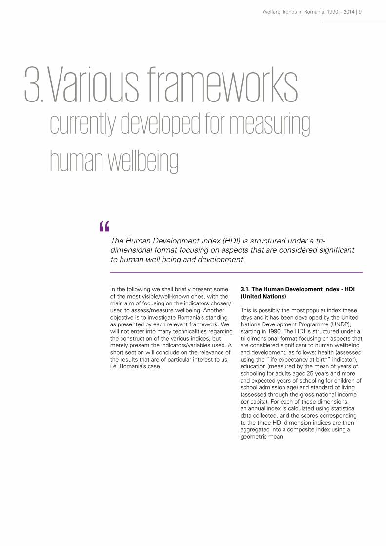
In the following we shall briefly present some of the most visible/well-known ones, with the main aim of focusing on the indicators chosen/used to assess/measure wellbeing. Another objective is to investigate Romania’s standing as presented by each relevant framework. We will not enter into many technicalities regarding the construction of the various indices, but merely present the indicators/variables used. A short section will conclude on the relevance of the results that are of particular interest to us, i.e. Romania’s case.
3.1. The Human Development Index - HDI (United Nations)
This is possibly the most popular index these days and it has been developed by the United Nations Development Programme (UNDP), starting in 1990. The HDI is structured under a tri-dimensional format focusing on aspects that are considered significant to human wellbeing and development, as follows: health (assessed using the “life expectancy at birth” indicator), education (measured by the mean of years of schooling for adults aged 25 years and more and expected years of schooling for children of school admission age) and standard of living (assessed through the gross national income per capita). For each of these dimensions, an annual index is calculated using statistical data collected, and the scores corresponding to the three HDI dimension indices are then aggregated into a composite index using a geometric mean.
The Human Development Index (HDI) is structured under a tri-dimensional format focusing on aspects that are considered significant to human well-being and development.
“
3. Various frameworks currently developed for measuring
human wellbeing

10 | Welfare Trends in Romania, 1990 – 2014
Figure 2HDI Components
Source: UNDP (2015), Human Development Report 2015. Work for Human Development, New York– Technical notes, p.1.
The 2015 HDI, the results of which we shall briefly present below, classifies countries under four major categories concerning human development: a) very high (HDI value ranging between 0.944 and 0.802), b) high (HDI value ranging between 0.798 and 0.702), c) medium (HDI value ranging between 0.698 and 0.555) and d) low (HDI value ranging between 0.548 and 0.348). The top three countries in the
latest 2014 rankings are Norway, Australia and Switzerland, while at the bottom of the list are the Central African Republic and Niger. In Figure 3 below we represent graphically Romania’s position as provided by the 2015 HDI scores, relative to other Central and East European (CEE) countries and one western society for a more relevant comparison.
Figure 3Ranking as per HDI score*
Source: Based on figures produced by UNDP (2015), Human Development Report 2015. Work for Human Development, New York, p. 208.
*based on 2014 figures
6
b) high (HDI value ranging between 0.798 and 0.702), c) medium (HDI value ranging between 0.698 and 0.555) and d) low (HDI value ranging between 0.548 and 0.348). The top three countries in the latest 2014 rankings are Norway, Australia and Switzerland, while at the bottom of the list are the Central African Republic and Niger. In Figure 3 below we represent graphically Romania’s position as provided by the 2015 HDI scores, relative to other neighbouring countries and one western society for a more relevant comparison.
Figure 3
Source: Based on figures produced by UNDP (2015), Human Development Report 2015. Work for Human Development, New York, p. 208. *based on 2014 figures Romania ranks 52 out of 188 countries analysed and it is positioned in the High Human Development category surpassing Bulgaria. However it is behind other CEE countries such as Hungary, Poland and the Czech Republic. By comparison, the scores obtained by these countries place them in the Very High Human Development category. It is important to notice, however, the dramatic development over time in Romania’s case, with an impressive advance recorded between the years 2000 and 2010 and slow, but ascendant, development until 2014.
Figure 4
Source: Based on figures produced by UNDP (2015), Human Development Report 2015. Work for Human Development, New York, p. 212.
0.70
0.75
0.80
0.85
0.90
0.95
Germany Czech Rep. Poland Hungary Romania Bulgaria
0.916
0.87
0.8430.828
0.7930.782
0.703 0.706
0.784 0.786 0.788 0.791 0.793
0.640.660.680.700.720.740.760.780.800.820.84
1990 2000 2010 2011 2012 2013 2014
HDI score trend for Romania

Welfare Trends in Romania, 1990 – 2014 | 11
3.2 The World Happiness Report - WHR (Sustainable Development Solutions Network)
The latest version of this report was published in 2016 (actually an update of the 2015 version). It was first produced in 2012 in the context of the United Nations High Level Meeting on “Happiness and Well-Being: Defining a New Economic Paradigm.”
The 2016 Report provides a country ranking which is constructed on both quantitative (mainly statistical) and qualitative (mainly surveys) factors. The qualitative component is based on survey data gathered under the Gallup World Poll (GWP). The specific analysis uses six key objective and subjective variables as follows6:
• GDP per capita;• Healthy life expectancy at birth;• Social Support;• Freedom to make life choices;• Generosity;• Perceptions of corruption.
According to the 2016 Report, Denmark, Switzerland and Iceland are top three countries, while Syria and Burundi are at the bottom of the ladder. Romania ranks 71 out of 157 countries reported. We provide below in Figure 5 a graphic representation of Romania’s standing in the World Happiness Report, by comparing the scores of other relevant countries (for consistency purposes we used the same country panel as in HDI’s case).
With a score of 5.528 Romania achieves a better standing compared to Hungary and Bulgaria, while the Czech Republic’s high score brings the latter closer to Germany than to its CEE peers.
Romania ranks 52 out of 188 countries analysed and it is positioned in the High Human Development category surpassing Bulgaria. However it is behind other CEE countries such as Hungary, Poland and the Czech Republic. By comparison, the scores obtained by these countries place them in the
Very High Human Development category. It is important to notice, however, the dramatic development over time in Romania’s case, with an impressive advance recorded between the years 2000 and 2010 and slow, but ascendant, development until 2014.
Figure 4HDI score trend for Romania
Source: Based on figures produced by UNDP (2015), Human Development Report 2015. Work for Human Development, New York, p. 212.
6
b) high (HDI value ranging between 0.798 and 0.702), c) medium (HDI value ranging between 0.698 and 0.555) and d) low (HDI value ranging between 0.548 and 0.348). The top three countries in the latest 2014 rankings are Norway, Australia and Switzerland, while at the bottom of the list are the Central African Republic and Niger. In Figure 3 below we represent graphically Romania’s position as provided by the 2015 HDI scores, relative to other neighbouring countries and one western society for a more relevant comparison.
Figure 3
Source: Based on figures produced by UNDP (2015), Human Development Report 2015. Work for Human Development, New York, p. 208. *based on 2014 figures Romania ranks 52 out of 188 countries analysed and it is positioned in the High Human Development category surpassing Bulgaria. However it is behind other CEE countries such as Hungary, Poland and the Czech Republic. By comparison, the scores obtained by these countries place them in the Very High Human Development category. It is important to notice, however, the dramatic development over time in Romania’s case, with an impressive advance recorded between the years 2000 and 2010 and slow, but ascendant, development until 2014.
Figure 4
Source: Based on figures produced by UNDP (2015), Human Development Report 2015. Work for Human Development, New York, p. 212.
0.70
0.75
0.80
0.85
0.90
0.95
Germany Czech Rep. Poland Hungary Romania Bulgaria
0.916
0.87
0.8430.828
0.7930.782
0.703 0.706
0.784 0.786 0.788 0.791 0.793
0.640.660.680.700.720.740.760.780.800.820.84
1990 2000 2010 2011 2012 2013 2014
HDI score trend for Romania
6. Helliwell, John F., Richard Layard, and Jeffrey Sachs, eds. (2016), World Happiness Report 2016 Update (Vol.I), New York, Sustainable Development Solutions Network, p. 17;

12 | Welfare Trends in Romania, 1990 – 2014
Figure 5Average 2013-2015 country score,
World Happiness Report
Source: Based on figures produced by Helliwell, John F., Richard Layard, and Jeffrey Sachs, eds. (2016), World Happiness Report 2016 Update (Vol. I), New York, Sustainable Development Solutions Network, pp.20-22.
7
3.2 The World Happiness Report (Sustainable Development Solutions Network) The latest version of this report was published in 2016 (actually an update of the 2015 version). It was first produced in 2012 in the context of the United Nations High Level Meeting on "Happiness and Well-Being: Defining a New Economic Paradigm." The 2016 Report provides a country ranking which is constructed on both quantitative (mainly statistical) and qualitative (mainly surveys) factors. The qualitative component is based on survey data gathered under the Gallup World Poll (GWP). The specific analysis uses six key objective and subjective variables as follows6: GDP per capita; Healthy life expectancy at birth; Social Support; Freedom to make life choices; Generosity; Perceptions of corruption.
According to the 2016 Report, Denmark, Switzerland and Iceland are top three countries, while Syria and Burundi are at the bottom of the ladder. Romania ranks 71 out of 157 countries reported. We provide below in Figure 5 a graphic representation of Romania’s standing in the World Happiness Report, by comparing the scores of other relevant countries (for consistency purposes we used the same country panel as in HDI’s case). With a score of 5.528 Romania achieves a better standing compared to Hungary and Bulgaria, while the Czech Republic’s high score brings the latter closer to Germany than to its CEE peers.
Figure 5
Source: Based on figures produced by Helliwell, John F., Richard Layard, and Jeffrey Sachs, eds. (2016), World Happiness Report 2016 Update (Vol. I), New York, Sustainable Development Solutions Network, pp.20-22. 3.3 The Legatum Prosperity Index (Legatum Institute) This is one of the most complex indices (if not “the” most complex) covering countries’ welfare and is based on both income (also taking into account the GDP factor) and other wellbeing indicators. From a methodological standpoint, it is a composite index based on nine sub-indices concerning7: Economic Quality; The Business Environment;
6 Helliwell, John F., Richard Layard, and Jeffrey Sachs, eds. (2016), World Happiness Report 2016 Update (Vol.I), New York, Sustainable Development Solutions Network, p. 17; 7 ––
0
1
2
3
4
5
6
7
Germany Czech Rep. Poland Romania Hungary Bulgaria
6.9946.596
5.835 5.5285.145
4.217
3.3 The Legatum Prosperity Index - LPI (Legatum Institute)
This is one of the most complex indices (if not “the” most complex) covering countries’ welfare and is based on both income (also taking into account the GDP factor) and other wellbeing indicators. From a methodological standpoint, it is a composite index based on nine sub-indices concerning7:
• Economic Quality;• The Business Environment;• Governance;• Education;• Health;• Safety and Security;
• Personal Freedom;• Social Capital;• Natural environment (introduced in 2016). The above sub-indices are based on a total of 104 variables which have been standardized and given weights through regression analysis. Each country analysed is ranked under a total score, as well as by scores assigned to each sub-index.
In the 2016 Legatum Prosperity Index Romania ranks 50 out of 149 countries analysed. The graphic below shows that its positioning relative to the CEE peers and Germany is not a favourable one, being the penultimate, after Bulgaria.
7. Legatum Institute (2016), The Legatum Prosperity Index 2016. Bringing prosperity to life, London, p. 4;

Welfare Trends in Romania, 1990 – 2014 | 13
Figure 7Legatum Prosperity Index: Romania’s score evolution
Source: Based on figures produced by the Legatum Institute (2016), The Legatum Prosperity Index 2016. Bringing prosperity to life, London – Prosperity rankings: Full data set.
8
Governance; Education; Health; Safety and Security; Personal Freedom; Social Capital; Natural environment (introduced in 2016).
The above sub-indices are based on a total of 104 variables which have been standardized and given weights through regression analysis. Each country analysed is ranked under a total score, as well as by scores assigned to each sub-index. In the 2016 Legatum Prosperity Index Romania ranks 50 out of 149 countries analysed. The graphic below shows that its positioning relative to the CEE peers and Germany is not a favourable one, being the penultimate, after Bulgaria.
Figure 6
Source: Based on figures produced by Legatum Institute (2016), The Legatum Prosperity Index 2016. Bringing prosperity to life, London – Prosperity rankings: Full data set . However, if we analyse the year-on-year development in Romania’s case, one can notice visible progress. After a drop in 2010-2011, a substantial score improvement started in 2012.
Figure 7
Source: Based on figures produced by the Legatum Institute (2016), The Legatum Prosperity Index 2016. Bringing prosperity to life, London – Prosperity rankings: Full data set.
0
10
20
30
40
50
60
70
80
Germany Czech rep. Poland Hungary Romania Bulgaria
76.8368.34 65.96 62.56 61.67 60.23
58.66 58.87 58.83
58.07 58.2758.96 59.23
60.52
61.67 61.67
5556575859606162636465
2007 2008 2009 2010 2011 2012 2013 2014 2015 2016
Legatum Prosperity Index: Romania's score evolution
Figure 6Legatum Prosperity Index score, 2016
Source: Based on figures produced by Legatum Institute (2016), The Legatum Prosperity Index 2016. Bringing prosperity to life, London – Prosperity rankings: Full data set
8
Governance; Education; Health; Safety and Security; Personal Freedom; Social Capital; Natural environment (introduced in 2016).
The above sub-indices are based on a total of 104 variables which have been standardized and given weights through regression analysis. Each country analysed is ranked under a total score, as well as by scores assigned to each sub-index. In the 2016 Legatum Prosperity Index Romania ranks 50 out of 149 countries analysed. The graphic below shows that its positioning relative to the CEE peers and Germany is not a favourable one, being the penultimate, after Bulgaria.
Figure 6
Source: Based on figures produced by Legatum Institute (2016), The Legatum Prosperity Index 2016. Bringing prosperity to life, London – Prosperity rankings: Full data set . However, if we analyse the year-on-year development in Romania’s case, one can notice visible progress. After a drop in 2010-2011, a substantial score improvement started in 2012.
Figure 7
Source: Based on figures produced by the Legatum Institute (2016), The Legatum Prosperity Index 2016. Bringing prosperity to life, London – Prosperity rankings: Full data set.
0
10
20
30
40
50
60
70
80
Germany Czech rep. Poland Hungary Romania Bulgaria
76.8368.34 65.96 62.56 61.67 60.23
58.66 58.87 58.83
58.07 58.2758.96 59.23
60.52
61.67 61.67
5556575859606162636465
2007 2008 2009 2010 2011 2012 2013 2014 2015 2016
Legatum Prosperity Index: Romania's score evolution
However, if we analyse the year-on-year development in Romania’s case, one can notice visible progress. After a drop in 2010-
2011, a substantial score improvement started in 2012.

14 | Welfare Trends in Romania, 1990 – 2014
Figure 8Country ranking as per HPI 2016 score
Source: Based on figures produced by New Economics Foundation (2016), “The Happy Planet Index 2016. A global index of sustainable wellbeing” – Data file.
9
3.4 The Happy Planet Index (New Economics Foundation) According to its own description, the Happy Planet Index (HPI) combines four elements in order to show how efficiently residents of different countries are using environmental resources to lead long, happy lives. It is a revolutionary tool in the sense that the rationale behind it is the need to develop a welfare measurement mechanism that takes into account sustainability indicators. Similarly to the World Happiness Report, the 2016 report includes both objective (quantitative) and subjective (qualitative) components, as follows8: Experienced wellbeing; Life expectancy; Inequality of outcomes; Ecological Footprint.
The HPI is not very complicated to calculate, the first three indicators are multiplied and the result is divided by the ecological footprint index9. In the 2016 HPI Report (the latest) Romania ranks 55 out of a total of 140 countries. When compared to the other group of countries already used for our analysis, Romania’s position is quite surprising (especially if we consider the results under the previous indices we have presented). As such, with a total score of 28.8 we are close to Germany and much better positioned when compared to Bulgaria or Hungary. Under this index, economically developed countries (such as Germany) score significantly below less developed states (for example, Luxembourg ranks 139 out of 140 countries). One of the main explanations for this is that, while having high life expectancy and scoring very well with regard to well-being, economically active countries have a correspondingly large ecological footprint which ultimately affects their final scoring.
Figure 8
Source:Based on figures produced by New Economics Foundation (2016), “The Happy Planet Index 2016. A global index of sustainable wellbeing” – Data file. 3.5 Preliminary conclusions In the above we have briefly examined quite a wide variety of frameworks, each providing their own vision on how to measure and report human prosperity and welfare. Featuring their own particularities, each focusing on a specific coordinate, the reports analysed are naturally separate reflections of the various interpretations of wellbeing, as described under Chapter 2 of this paper. So what conclusions 8 New Economics Foundation (2016), The Happy Planet Index 2016. A global index of sustainable wellbeing – Briefing paper, p. 1; Methods paper, p. 2-9. 9 New Economics Foundation (2016), The Happy Planet Index 2016. A global index of sustainable wellbeing – Methods paper, p. 1.
0
5
10
15
20
25
30
Germany Romania Poland Czech Rep. Hungary Bulgaria
29.8 28.8 27.5 27.3 26.4
20.4
3.4 The Happy Planet Index - HPI (New Economics Foundation)
According to its own description, the Happy Planet Index (HPI) combines four elements in order to show how efficiently residents of different countries are using environmental resources to lead long, happy lives. It is a revolutionary tool in the sense that the rationale behind it is the need to develop a welfare measurement mechanism that takes into account sustainability indicators. Similarly to the World Happiness Report, the 2016 report includes both objective (quantitative) and subjective (qualitative) components, as follows8:• Experienced wellbeing;• Life expectancy;• Inequality of outcomes;• Ecological Footprint.The HPI is not very complicated to calculate, the first three indicators are multiplied and the result is divided by the ecological footprint index9.
In the 2016 HPI Report (the latest) Romania ranks 55 out of a total of 140 countries. When compared to the other group of countries already used for our analysis, Romania’s position is quite surprising (especially if we consider the results under the previous indices we have presented). As such, with a total score of 28.8 we are close to Germany and much better positioned when compared to Bulgaria or Hungary.
Under this index, economically developed countries (such as Germany) score significantly below less developed states (for example, Luxembourg ranks 139 out of 140 countries). One of the main explanations for this is that, while having high life expectancy and scoring very well with regard to well-being, economically active countries have a correspondingly large ecological footprint which ultimately affects their final scoring.
8. New Economics Foundation (2016), The Happy Planet Index 2016. A global index of sustainable wellbeing – Briefing paper, p. 1; Methods paper, pp. 2-9;
9. New Economics Foundation (2016), The Happy Planet Index 2016. A global index of sustainable wellbeing – Methods paper, p. 1.;

Welfare Trends in Romania, 1990 – 2014 | 15
Figure 9Romania’s rankings according to various welfare reports
Source: Based on figures produced by the Human Development Index (HDI) 2015; World Happiness Report (WHR) 2016; Legatum Prosperity Index (LPI) 2016; Happy Planet Index (HPI) 2016.
9
3.4 The Happy Planet Index (New Economics Foundation) According to its own description, the Happy Planet Index (HPI) combines four elements in order to show how efficiently residents of different countries are using environmental resources to lead long, happy lives. It is a revolutionary tool in the sense that the rationale behind it is the need to develop a welfare measurement mechanism that takes into account sustainability indicators. Similarly to the World Happiness Report, the 2016 report includes both objective (quantitative) and subjective (qualitative) components, as follows8: Experienced wellbeing; Life expectancy; Inequality of outcomes; Ecological Footprint.
The HPI is not very complicated to calculate, the first three indicators are multiplied and the result is divided by the ecological footprint index9. In the 2016 HPI Report (the latest) Romania ranks 55 out of a total of 140 countries. When compared to the other group of countries already used for our analysis, Romania’s position is quite surprising (especially if we consider the results under the previous indices we have presented). As such, with a total score of 28.8 we are close to Germany and much better positioned when compared to Bulgaria or Hungary. Under this index, economically developed countries (such as Germany) score significantly below less developed states (for example, Luxembourg ranks 139 out of 140 countries). One of the main explanations for this is that, while having high life expectancy and scoring very well with regard to well-being, economically active countries have a correspondingly large ecological footprint which ultimately affects their final scoring.
Figure 8
Source:Based on figures produced by New Economics Foundation (2016), “The Happy Planet Index 2016. A global index of sustainable wellbeing” – Data file. 3.5 Preliminary conclusions In the above we have briefly examined quite a wide variety of frameworks, each providing their own vision on how to measure and report human prosperity and welfare. Featuring their own particularities, each focusing on a specific coordinate, the reports analysed are naturally separate reflections of the various interpretations of wellbeing, as described under Chapter 2 of this paper. So what conclusions 8 New Economics Foundation (2016), The Happy Planet Index 2016. A global index of sustainable wellbeing – Briefing paper, p. 1; Methods paper, p. 2-9. 9 New Economics Foundation (2016), The Happy Planet Index 2016. A global index of sustainable wellbeing – Methods paper, p. 1.
0
5
10
15
20
25
30
Germany Romania Poland Czech Rep. Hungary Bulgaria
29.8 28.8 27.5 27.3 26.4
20.4
10
each focusing on a specific coordinate, the reports analysed are naturally separate reflections of the various interpretations of wellbeing, as described under Chapter 2 of this paper. So what conclusions can we draw after going through this selection? First of all, what all frameworks have in common is that they all use additional measurement factors besides income. These factors are both quantitative (i.e. statistical indicators such as life expectancy at birth or years of schooling) and qualitative (such as people’s perception on corruption). This is a clear indicator that the latest trends in assessing human welfare are focused more and more on including societal aspects into the welfare measurement equation. As expected, the results in terms of country ranking are not identical. However, one can notice a recurrent pattern in that the top ten countries is generally composed of the same “usual suspects”, such as Norway, Sweden, Finland, Switzerland, Netherlands or Australia. The same pattern is consistent when we look at those states forming the bottom of the ladder, usually African countries such as Niger, Togo, Chad or Central-African Republic. An exception however is the HPI, given the methodological reasons already presented. Its results taken at face value may seem controversial (ranking the US on the 108th position, next to Bulgaria, is a good example in this respect). But then again we need to turn to the rationale and methodology used by this index. Can anyone really argue with the fact that a sustainable use of natural resources and a clean and healthy environment are absolute prerequisites of future human welfare? The HPI’s measurement tool clearly goes to prove that the results of any study on wellbeing measurement largely depends on the indicators used and, ultimately, on the goal of each individual piece of research. As such, one should not attempt to interpret the results of various studies in a comparative manner, but rather try to understand the objectives of each index, as well as the context in/for which they were developed. With regard to Romania’s standing however, across the studies presented, the relative ranking seems to be constantly close to the first third of the league, as the graph below represents. Although we advised against cross interpretation between various reports with regard to a specific country/ies, the empirical ascertainment related to Romania’s similar ranking in all four reports quoted is quite remarkable.
Figure 9
Source: Based on figures produced by the Human Development Index (HDI) 2015; World Happiness Report (WHR) 2016; Legatum Prosperity Index (LPI) 2016; Happy Planet Index (HPI) 2016. The following chapter of this study will detail the development of some wellbeing indicators for Romania and other CEE countries, in order to emphasize more relevantly the main trends and provide some explanations. We will limit our investigation to the year 2014, which is the last available for some indicators. 4. Welfare Trends in Romania and other CEE countries during 1990-2014
52
71
50
55
HDI (2014), 188 countries
WHR (2013-2015), 157 countries
LPI (2016), 149 countries
HPI (2016), 140 countries
Romania's rankings according to various welfare reports
3.5 Preliminary conclusions
In the above we have briefly examined quite a wide variety of frameworks, each providing their own vision on how to measure and report human prosperity and welfare. Featuring their own particularities, each focusing on a specific coordinate, the reports analysed are naturally separate reflections of the various interpretations of wellbeing, as described under Chapter 2 of this paper. So what conclusions can we draw after going through this selection?
First of all, what all frameworks have in common is that they all use additional measurement factors besides income. These factors are both quantitative (i.e. statistical indicators such as life expectancy at birth or years of schooling) and qualitative (such as people’s perception on corruption). This is a clear indicator that the latest trends in assessing human welfare are focused more and more on including societal aspects into the welfare measurement equation.
As expected, the results in terms of country ranking are not identical. However, one can notice a recurrent pattern in that the top ten countries is generally composed of the same “usual suspects”, such as Norway, Sweden, Finland, Switzerland, Netherlands or Australia. The same pattern is consistent when we look at those states forming the bottom of the ladder, usually African countries such as Niger, Togo, Chad or Central-African Republic.
An exception however is the HPI, given the methodological reasons already presented. Its results taken at face value may seem controversial (ranking the US on the 108th position, next to Bulgaria, is a good example in this respect). But then again we need to turn to the rationale and methodology used by this index. Can anyone really argue with the fact that a sustainable use of natural resources and a clean and healthy environment are absolute prerequisites of future human welfare?
The HPI’s measurement tool clearly goes to prove that the results of any study on wellbeing measurement largely depends on the indicators used and, ultimately, on the goal of each individual piece of research. As such, one should not attempt to interpret the results of various studies in a comparative manner, but rather try to understand the objectives of each index, as well as the context in/for which they were developed.
With regard to Romania’s standing however, across the studies presented, the relative ranking seems to be constantly close to the first third of the league, as the graph below represents. Although we advised against cross interpretation between various reports with regard to a specific country/ies, the empirical ascertainment related to Romania’s similar ranking in all four reports quoted is quite remarkable.
The following chapter of this study will detail the development of some wellbeing indicators for Romania and other CEE countries, in order to emphasize more relevantly the main trends
and provide some explanations. We will limit our investigation to the year 2014, which is the last available for some indicators.

16 | Welfare Trends in Romania, 1990 – 2014
As presented in the theoretical section, the concept of welfare includes quite a variety of life quality aspects, corresponding to different theories in the literature. In this study our aim is to follow a pragmatic and hedonic approach to the mentioned concept, in the sense that we are interested in measuring the satisfaction of basic needs, corresponding mainly to the first two levels of the well-known pyramid of human needs, as outlined by Abraham Maslow. We will not analyze those aspects of welfare related to social, cultural, or spiritual needs, as we believe that these are difficult to quantify and very different from one person to another, or even absent in some people. On the other hand, we intend to carry out a welfare analysis in the objective sense, measured by quantitative data. The subjective analysis of wellbeing, consisting of perceptions of each individual on the satisfaction provided by various sides of life, is not the subject of our survey.
We deal in this chapter with the following three pillars of welfare: health, income and consumption, as well as education. Unlike other frameworks on this topic (HDI10, MPI11, HPI12, WHR13, etc.) which built classifications of countries on various criteria, at some point in time,
our paper is focused on the long-term dynamics of living standards, for each country considered. First, we study, comparatively, how different indicators of well-being have varied in five Central and Eastern European countries (CEE), i.e. Romania, Bulgaria, the Czech Republic, Hungary and Poland, and one Western European developed country (as a benchmark for comparison) – Germany - during two and a half decades, i.e. from 1990 to 2014. We chose 1990 as a base year for measuring welfare dynamics because it is a milestone in the economic development of the CEE countries, i.e. the turning point from the centralised system to the free market economy.
Second, we provide an overview of their dynamics during the period 1990-2014. Because the relevant time variations have different ranges, a composite index summing up the dynamics for each country would be inappropriate. This is why we will use a radar-type chart instead, providing the 1990-2014 indicator normalized changes corresponding to the 5+1 countries. We end this chapter with the development of welfare gaps between Romania and the other countries considered, during the mentioned period.
We chose 1990 as a base year for measuring welfare dynamics because it is a milestone in the economic development of the CEE countries, i.e. the turning point from the centralised system to the free market economy.
“
4. Welfare Trends
in Romania and other CEE countries
during 1990-2014
10. Human Development Index;11. Multidimensional Poverty Index;12. Happy Planet Index;13. World Happiness Report;

Welfare Trends in Romania, 1990 – 2014 | 17
The following sections of this chapter include: the methodology and data used (section 4.1), the statistical analysis of the proposed welfare indicators (section 4.2), and the big picture of welfare dynamics and welfare gaps during 1990-2014 (section 4.3).
4.1. Methodology and data used
Because of the rather long period for which we intend to study the development of welfare, the range of available and relevant statistical indicators, corresponding to all countries analysed, is quite limited. Out of the open access statistical databases providing 1990-2014 data, the only complete data series were found with the World Bank (WB)14 and Penn World Table (PWT)15. We added to these series other indicators that we deemed as being significant for the description of the analyzed aspects, although they are available for shorter time periods. Annex 1 combines the indicators used in this study, their measure units and sources of statistical data used for their accession.
4.1.1. Health
We start with the population’s health status, which we consider to be a core component of a nation’s welfare. Health is our most valuable asset since a good physical and mental state is crucial for being able to work, study and enjoy life. Assessing health status, however, is a difficult task because of the multitude of aspects involved. Limited long-term data available constrained us to limit our analysis to certain indicators. The ones we have chosen, available for the period 1990 – 2014, are: life expectancy at birth, expressed in number of years (calculated by WB) and infant survival rate, per thousand live births (obtained through the difference to 1,000 of infant mortality, also calculated by WB).
4.1.2. Income
Although the use of GDP in welfare evaluation is increasingly controversial, revenues of companies active within a country in exchange for products and services provided can be considered a proxy for the population’s income.
We will start to estimate income progress by examining historical GDP for Romania, as calculated by Victor Axenciuc (2012)16. This data series ends in the year 2000, but we have extended it to year 2015 using a volume index provided by Eurostat. Further, for all six countries analyzed, we have chosen GDP per capita provided by the WB, expressed in 2011 USD constant prices at purchasing power parity (PPP).
We will later compare the GDP with the gross national income (GNI). National income is obtained by extracting from the GDP the difference between primary incomes (employees’ compensation and property income: dividends, interest, rent, and retained profit) achieved by foreign entities in the country and the incomes achieved by residents on the territory of other countries17. The two components may balance each other out, so that GNI and GDP levels are very close. However, this is not the case for the CEE countries, where the first component - incomes of foreigners operating within the country’s borders - is substantial, while the latter is usually small. Consequently, their national income is noticeably lower than domestic product, as we will see by calculating the ratio of GNI to GDP. Thus, although foreign companies may boost economic growth (GDP), their contribution to national income (GNI) is usually smaller. To calculate the mentioned ratio, we used GDP and GNI in current national currency, also available on the WB database.
Revenue data represent national average values, which say nothing about their distribution to individuals. For this purpose we used WB estimates of the Gini index based on household surveys, which quantifies “the extent to which the distribution of income (or, in some cases, consumption expenditure) among individuals or households within an economy deviates from a perfectly equal distribution.(...) a Gini index of 0 represents perfect equality, while an index of 100 implies perfect inequality”18.
14. http://data.worldbank.org/indicator;15. Feenstra, Robert C., Robert Inklaar and Marcel P. Timmer (2015), The Next Generation of the
Penn World Table American Economic Review, 105(10), 3150-3182, available for download at www.ggdc.net/pwt;
16. Axenciuc, V. (2012), Produsul intern brut al României 1862-2000. Serii statistice seculare și argumente metodologice, volumul I: Produsul intern brut 1862-2000. Sinteza seriilor de timp a indicatorilor globali, pe secțiuni temporale, Editura Economică, București, 2012, pp. 38-41;
17. For more details see the OECD definition: https://data.oecd.org/natincome/gross-national-income.htm;
18. http://data.worldbank.org/indicator/SI.POV.GINI;

18 | Welfare Trends in Romania, 1990 – 2014
4.1.3. Consumption
Consumption is another widely-used measure for standard of living, reflecting the hedonic side of welfare, namely the satisfaction obtained by spending revenue and other financial resources (e.g. loans). Obviously, consumption largely depends on the temperament and life philosophy of each person which, alongside with rational factors19 generate the distribution of financial resources towards consumption and saving. A relatively higher consumption level does not necessarily mean a higher level of wellbeing, but rather an excessive propensity to capitalize on present and/or future earnings in order to maximize present satisfaction.
We will consider the final consumption of households20, per capita, expressed in 2011 USD PPP, which was calculated based on the same indicator expressed in constant 2010 USD. This series was first converted to constant 2011 national currency, using the 2010 exchange rate (national currency / USD) and national consumer price index for 2011 (2010=100). Second, it was converted to 2011 USD PPP, using the 2011 PPP conversion factor. All the above indicators were available in the WB data base.
4.1.4. Education
The role of education in improving welfare resides in both its contribution to personal development as well as the facilitation of higher earnings in
the labour market. We will analyze the level of education using the human capital index (HCI)21 conducted by PWT alongside with tertiary enrolment ratio provided by the WB. HCI per person is calculated based on the number of years of schooling and its marginal rate of return. The latter is given by a coefficient calculated as a Mincer-type function of incomes, where the income of an individual is correlated with the degree of education. The coefficient is different on various segments of the educational route. Tertiary enrolment ratio (WB) is calculated as the percentage of people enrolled in tertiary education within the total number of persons in the age group (within 5 years) corresponding to the period subsequent to the graduation of secondary school.
4.2. Main findings
4.2.1. Health
In order to analyse the health status of a population, we considered two indicators: life expectancy at birth (years) and infant survival rate (‰) - calculated by the difference to 1,000 of WB infant mortality (‰). In Figures 10a-10b, we showed the development of these indicators over the 1990-2014 period, for 5 CEE emerging economies (Romania, Poland, Hungary, Bulgaria and the Czech Republic) to which we added a West-European developed country (Germany).
19. See the intertemporal consumption theories and life-cycle model of consumption;20. Household consumption include expenditures of nonprofit institutions serving
households, as mentioned by the WB (http://data.worldbank.org/indicator/NE.CON.PRVT.PC.KD?view=chart);
21. http://www.rug.nl/ggdc/docs/human_capital_in_pwt_90.pdf;
Figure 10aLife expectancy at birth (years)
Source: World Bank Indicators.
13
well as the facilitation of higher earnings in the labour market. We will analyze the level of education using the human capital index21 (HCI) conducted by PWT alongside with tertiary enrolment ratio provided by the WB. HCI per person is calculated based on the number of years of schooling and its marginal rate of return. The latter is given by a coefficient (quite relatively) calculated as a Mincer-type function of incomes, where the income of an individual is correlated with the degree of education. The coefficient is different on various segments of the educational route. Tertiary enrolment ratio (WB) is calculated as the percentage of people enrolled in tertiary education within the total number of persons in the age group (within 5 years) corresponding to the period subsequent to the graduation of secondary school. 4.2. Main findings
4.2.1. Health
In order to analyse the health status of a population, we considered two indicators: life expectancy at birth (years) and infant survival rate (‰) - calculated by the difference to 1,000 of WB infant mortality (‰). In Figures 10a-10b, we showed the development of these indicators over the 1990-2014 period, for 5 CEE emerging economies (Romania, Poland, Hungary, Bulgaria and the Czech Republic) to which we added a West-European developed country (Germany), as a benchmark for comparisons.
Figure 10a
Source: World Bank Indicators. Figure 10a shows that the ‘90s brought a significant overall increase in life expectancy in all CEE countries considered, which lasts until the end of the period. This may be interpreted in the sense that the economic changes that occurred after 1990 have had a positive effect on the health system and hence on the population’s health condition. The absolute rise in life expectancy in Romania was 5.3 years, during 1990-2014. Noteworthy is that the 5+1 country trends are parallel as of 1990, although Romania and Bulgaria have a late start (1998). Figure 10b shows that the number of children who survive to the age of 1 year, per thousand live births in the respective year (infant survival rate) has also increased considerably. Romania’s values marginally decreased during the late 2000s, along with the other countries. Its 1990-2014 rise (20.9 ‰) was the highest within the CEE group. Germany recorded only a modest rise, but only because its absolute values were net superior to the CEE countries, so the growth potential was inferior.
21 http://www.rug.nl/ggdc/docs/human_capital_in_pwt_90.pdf
68
70
72
74
76
78
80
82
1990
1991
1992
1993
1994
1995
1996
1997
1998
1999
2000
2001
2002
2003
2004
2005
2006
2007
2008
2009
2010
2011
2012
2013
2014
Life expectancy at birth (years)
Romania BulgariaCzech Rep. HungaryPoland Germany

Welfare Trends in Romania, 1990 – 2014 | 19
Figure 10a shows that the ‘90s brought a significant overall increase in life expectancy in all CEE countries considered, which lasts until the end of the period. This may be interpreted in the sense that the economic changes that occurred after 1990 have had a positive effect on the health system and hence on the population’s health condition. The absolute rise in life expectancy in Romania was 5.3 years, during 1990-2014. Noteworthy is that the 5+1 country trends are almost parallel, although Romania and Bulgaria have a late start (1998).
Figure 10b shows that the number of children who survive to the age of 1 year, per thousand live births in the respective year (infant survival rate) has also increased considerably. Romania’s values marginally decreased during the late 2000s, along with the other countries. Its 1990-2014 rise (20.9 ‰) was the highest within the CEE group. Germany recorded only a modest rise, but only because its absolute values were superior to the CEE countries, so the growth potential was inferior.
Figure 10bSurvival rate, infant (per 1,000 live births)
Source: Own calculation, based on World Bank Indicators.
14
Figure 10b
Source: World Bank Indicators.
4.2.2. Income
In this sub-section we will first review the GDP historical series for Romania (1950-2000), expressed in constant USD PPP, as calculated by Axenciuc (2012). We extended this series up to 2015, using a chained linked volume index provided by Eurostat.
Figure 11a
Source: Figures provided by Axenciuc (2012, p. 38-41), and own calculations based on Axenciuc (2012) and Eurostat. Data reveal that the post Second World War period brought a substantial real GDP upswing, with a peak in 1987, meaning that the GDP decline occurred before the economic transformations which started in 1989. This inflexion can be seen as part of the business cycle, or as a signal that the performance of the Romanian centralized economy might have come to a critical moment (an argument may be that a turning point had already happened in 1984). Further, the graph shows that the transition to the market economy had a strong impact on economic growth. Nevertheless, after a second downward trend in the 1997–1999 period, Romania’s real GDP growth has enjoyed the steepest upturn since 1950, interrupted only by the shock of the global crisis (2009-2010). According to our figures, extended based on the Axenciuc (2012) data series, the 2015 real GDP value was 1.5 times higher than the 1987 peak, and 11.5 times higher than the 1950 value.
965
970
975
980
985
990
995
1000
1990
1991
1992
1993
1994
1995
1996
1997
1998
1999
2000
2001
2002
2003
2004
2005
2006
2007
2008
2009
2010
2011
2012
2013
2014
Survival rate, infant (per 1,000 live births)
RomaniaBulgariaCzech Rep.HungaryPolandGermany
02,0004,0006,0008,000
10,00012,00014,00016,00018,000
1950
1952
1954
1956
1958
1960
1962
1964
1966
1968
1970
1972
1974
1976
1978
1980
1982
1984
1986
1988
1990
1992
1994
1996
1998
2000
2002
2004
2006
2008
2010
2012
2014
GDP per capita in Romania, 1950 - 2015, 2000 USD PPP
Axenciuc (2012) original GDP series
2001 - 2015 extended series, based onEurostat chained linked volume index

20 | Welfare Trends in Romania, 1990 – 2014
4.2.2. Income
In this sub-section we will first review the GDP historical series for Romania (1950-2000),
expressed in constant USD PPP, as calculated by Axenciuc (2012). We extended this series up to 2015, using a chained linked volume index provided by Eurostat.
Data reveal that the post Second World War period brought a substantial real GDP upswing, with a peak in 1987, meaning that the GDP decline occurred before the economic transformations which started in 1989. This inflexion can be seen as part of the business cycle, or as a signal that the performance of the Romanian centralized economy might have come to a critical moment (an argument may be that a turning point had already happened in 1984).
Further, the graph shows that the transition to the market economy had a strong impact on economic growth. Nevertheless, after a second downward trend in the 1997–1999 period, Romania’s real GDP growth has enjoyed the steepest upturn since 1950, interrupted only by the shock of the global crisis (2009-2010). According to our figures,
extended based on the Axenciuc (2012) and Eurostat data series, the 2015 real GDP value was 1.5 times higher than the 1987 peak, and 11.5 times higher than the 1950 value.In order to analyse all the CEE countries considered we use WB data, i.e. GDP per capita expressed in USD at PPP, 2011 constant prices. In figures 11b and 11c we combined the GDP absolute and relative (1991 base year) dynamics. In absolute terms, Romania’s GDP has been the second lowest among the group since 1992. After two declines recorded in 1992 and 1997-1999, its GDP did not reach the 1990 level until 2002. The increase became more robust from 2000, but it gained momentum particularly within the 2005 – 2008 period, supported by both domestic and external demand. However, the impact of the global crisis drastically adjusted the GDP path.
Figure 11aGDP per capita in Romania, 1950 - 2015, 2000 USD PPP
Source: Figures provided by Axenciuc (2012, pp. 38-41), and own calculations based on Axenciuc (2012) and Eurostat.
14
Figure 10b
Source: World Bank Indicators.
4.2.2. Income
In this sub-section we will first review the GDP historical series for Romania (1950-2000), expressed in constant USD PPP, as calculated by Axenciuc (2012). We extended this series up to 2015, using a chained linked volume index provided by Eurostat.
Figure 11a
Source: Figures provided by Axenciuc (2012, p. 38-41), and own calculations based on Axenciuc (2012) and Eurostat. Data reveal that the post Second World War period brought a substantial real GDP upswing, with a peak in 1987, meaning that the GDP decline occurred before the economic transformations which started in 1989. This inflexion can be seen as part of the business cycle, or as a signal that the performance of the Romanian centralized economy might have come to a critical moment (an argument may be that a turning point had already happened in 1984). Further, the graph shows that the transition to the market economy had a strong impact on economic growth. Nevertheless, after a second downward trend in the 1997–1999 period, Romania’s real GDP growth has enjoyed the steepest upturn since 1950, interrupted only by the shock of the global crisis (2009-2010). According to our figures, extended based on the Axenciuc (2012) data series, the 2015 real GDP value was 1.5 times higher than the 1987 peak, and 11.5 times higher than the 1950 value.
965
970
975
980
985
990
995
1000
1990
1991
1992
1993
1994
1995
1996
1997
1998
1999
2000
2001
2002
2003
2004
2005
2006
2007
2008
2009
2010
2011
2012
2013
2014
Survival rate, infant (per 1,000 live births)
RomaniaBulgariaCzech Rep.HungaryPolandGermany
02,0004,0006,0008,000
10,00012,00014,00016,00018,000
1950
1952
1954
1956
1958
1960
1962
1964
1966
1968
1970
1972
1974
1976
1978
1980
1982
1984
1986
1988
1990
1992
1994
1996
1998
2000
2002
2004
2006
2008
2010
2012
2014
GDP per capita in Romania, 1950 - 2015, 2000 USD PPP
Axenciuc (2012) original GDP series
2001 - 2015 extended series, based onEurostat chained linked volume index

Welfare Trends in Romania, 1990 – 2014 | 21
Relative dynamics is more meaningful when analysing GDP development as it compares its absolute changes to the initial value, i.e., the size of the economy. Also from the income point of view, its marginal utility is dependant on the initial level. Figure 11c below reveals that throughout the period 1991 - 2014 (Hungary’s 1990 GDP value is missing, consequently we chose 1991 as the base year) Poland leads the group as regards relative
growth, followed by Romania and Bulgaria. Poland’s GDP has increased to an extent far greater than that of the other states, recording a level in 2014 which was approximately 2.5 times higher than in 1991. Moreover, Poland is the only country where the effect of global crisis was almost absent. On the other hand, Romania was visibly affected, and consequently real GDP in 2014 was only 1.9 times higher than in 1991.
Figure 11bGDP per capita, 2011 USD PPP
Figure 11cGDP per capita, 1991=1
Source: World Bank Indicators
Source: own calculations, based on World Bank Indicators.15
In order to analyse all the CEE countries considered we use WB data, i.e. GDP per capita expressed in USD at PPP, 2011 constant prices. In figures 11b and 11c we combined the GDP absolute and relative (1991 base year) dynamics, for the same group of countries. In absolute terms, Romania’s GDP has been the second lowest among the group since 1992. Its GDP, after two declines recorded in 1992 and 1999, did not reach the 1990 level until 2002. The increase became more robust from 2000, but it gained momentum particularly within the 2005 – 2008 period, supported by both domestic demand and exports. However, the impact of the global crisis drastically adjusted the GDP path.
Figure 11b
Source: World Bank Indicators. Relative dynamics is more meaningful when analysing GDP development as it compares its absolute changes to the initial level, i.e., the size of the economy. Figure 11c below reveals that throughout the period 1990 - 2014 Poland leads the group as regards relative growth, followed by Romania and Bulgaria. Poland’s GDP has increased to an extent far greater than that of the other states, recording a level in 2014 which was approximately 2.5 times higher than in 1991. Moreover, Poland is the only country where the effect of global crisis was almost absent. On the other hand, Romania was visibly affected, and consequently real GDP in 2014 was only 1.9 times higher than in 1991.
Figure 11c
Source: own calculations, based on World Bank Indicators.
0
5,000
10,000
15,000
20,000
25,000
30,000
35,000
40,000
45,000
50,000
1990
1991
1992
1993
1994
1995
1996
1997
1998
1999
2000
2001
2002
2003
2004
2005
2006
2007
2008
2009
2010
2011
2012
2013
2014
GDP per capita, 2011 USD PPP
Romania Bulgaria Czech Rep.Hungary Poland Germany
0.8
1.0
1.2
1.4
1.6
1.8
2.0
2.2
2.4
2.6
1991
1992
1993
1994
1995
1996
1997
1998
1999
2000
2001
2002
2003
2004
2005
2006
2007
2008
2009
2010
2011
2012
2013
2014
GDP per capita, 1991=1
RomaniaBulgariaCzech Rep.HungaryPolandGermany
15
In order to analyse all the CEE countries considered we use WB data, i.e. GDP per capita expressed in USD at PPP, 2011 constant prices. In figures 11b and 11c we combined the GDP absolute and relative (1991 base year) dynamics, for the same group of countries. In absolute terms, Romania’s GDP has been the second lowest among the group since 1992. Its GDP, after two declines recorded in 1992 and 1999, did not reach the 1990 level until 2002. The increase became more robust from 2000, but it gained momentum particularly within the 2005 – 2008 period, supported by both domestic demand and exports. However, the impact of the global crisis drastically adjusted the GDP path.
Figure 11b
Source: World Bank Indicators. Relative dynamics is more meaningful when analysing GDP development as it compares its absolute changes to the initial level, i.e., the size of the economy. Figure 11c below reveals that throughout the period 1990 - 2014 Poland leads the group as regards relative growth, followed by Romania and Bulgaria. Poland’s GDP has increased to an extent far greater than that of the other states, recording a level in 2014 which was approximately 2.5 times higher than in 1991. Moreover, Poland is the only country where the effect of global crisis was almost absent. On the other hand, Romania was visibly affected, and consequently real GDP in 2014 was only 1.9 times higher than in 1991.
Figure 11c
Source: own calculations, based on World Bank Indicators.
0
5,000
10,000
15,000
20,000
25,000
30,000
35,000
40,000
45,000
50,000
1990
1991
1992
1993
1994
1995
1996
1997
1998
1999
2000
2001
2002
2003
2004
2005
2006
2007
2008
2009
2010
2011
2012
2013
2014
GDP per capita, 2011 USD PPP
Romania Bulgaria Czech Rep.Hungary Poland Germany
0.8
1.0
1.2
1.4
1.6
1.8
2.0
2.2
2.4
2.6
1991
1992
1993
1994
1995
1996
1997
1998
1999
2000
2001
2002
2003
2004
2005
2006
2007
2008
2009
2010
2011
2012
2013
2014
GDP per capita, 1991=1
RomaniaBulgariaCzech Rep.HungaryPolandGermany

22 | Welfare Trends in Romania, 1990 – 2014
Because a significant part of the revenues realised by foreign companies, resident in the CEE countries, leave the national economies, a more suitable indicator for assessing people’s welfare is national income (WB), because this removes from GDP primary incomes achieved by foreign entities across the country, and adds the incomes received from abroad (please refer to section 4.1.2 above for a review of this indicator).
In figure 11d we can observe that the GNI-GDP ratio in the CEE countries is below 100% for most of the countries, and it goes down to 92.4% (Czech Republic, 2011). During the
second half of the analyzed period, we may say that the ratio tendency is rather similar from one CEE country to another, except for the Czech Republic and some oscillations for Bulgaria. The rise in foreign direct investment led to a decrease in this ratio from 2000. However, after 2007 (earlier in Romania, later in the Czech Republic), an upward trend occurred, which may signal a decline in the activity of foreign companies. Germany has an opposite trend, i.e. it has benefited from above 100% values after 2004, meaning that incomes received from abroad have been higher than foreigners’ incomes in the country.
Further, in order to assess the extent to which income inequality has developed over time we present the development of the Gini index, as estimated by the WB based on household
surveys (please refer to section 4.1.2 above for a concept refresh). Because the data for 1990 was missing, we selected 1989 as the start year.
Despite different developments for the countries selected, the tendency towards growth of income inequality is obvious. If we compare 1989 and 2012 values, Bulgaria and Romania register the most sizable growth
of income inequality (12.6 p.p. and 11.6 p.p., respectively). In the Czech Republic and Hungary we notice a decreasing trend after 2004; also in Romania, after a maximum in 2008 (36.9%), the 2012 value is 2.1 p.p. lower.
Figure 11dGNI, % of GDP
Source: own calculation, based on World Bank Indicators.
16
Because a significant part of the revenues realised by foreign companies, resident in the CEE countries, leave the national economies, a more suitable indicator for assessing people’s welfare is national income (WB), because this removes from GDP primary incomes achieved by foreign companies across the country, which is a significant component in the CEE countries (please refer to section 4.1.2 above for a review of this indicator). In figure 11d we can observe that the GNI-GDP ratio in the CEE countries is below 100% for most of the countries, and it goes down to 92.4% (Czech Republic, 2011). Except for the Czech Republic and some oscillations for Bulgaria, we may say that the ratio is similar from one CEE country to another, both in terms of level and tendency. The rise in foreign direct investment led to a decrease in this ratio from 2000. However, after 2007 (earlier in Romania, later in the Czech Republic), an upward trend occurred, which may signal a decline in the activity of foreign companies. Germany has an opposite trend, i.e. it has benefited from above 100% values after 2004, meaning that incomes received from abroad have been higher than foreigners’ incomes in the country.
Figure 11d
Source: own calculation, based on World Bank Indicators. Further, in order to assess the extent to which income inequality has developed over time we present the development of the Gini index, as estimated by the WB based on household surveys (please refer to section 4.1.2 above for a concept refresh). Because the data for 1990 was missing, we selected 1989 as the start year.
Figure 11e
* 1988 for the Czech Republic; **2003 for Bulgaria. Note: data not available for Germany. Source: World Bank Indicators.
90
95
100
105
1990
1991
1992
1993
1994
1995
1996
1997
1998
1999
2000
2001
2002
2003
2004
2005
2006
2007
2008
2009
2010
2011
2012
2013
2014
GNI, % of GDP
Romania
Bulgaria
Czech Rep.
Hungary
Poland
Germany
0
10
20
30
40
Bulgaria Czech Rep. Hungary Poland Romania
Gini index, %
1989 * 2004** 2008 2012
Figure 11eGini index, %
* 1988 for the Czech Republic; **2003 for Bulgaria. Note: Germany was excepted because complete data was not available.Source: World Bank Indicators.
16
Because a significant part of the revenues realised by foreign companies, resident in the CEE countries, leave the national economies, a more suitable indicator for assessing people’s welfare is national income (WB), because this removes from GDP primary incomes achieved by foreign companies across the country, which is a significant component in the CEE countries (please refer to section 4.1.2 above for a review of this indicator). In figure 11d we can observe that the GNI-GDP ratio in the CEE countries is below 100% for most of the countries, and it goes down to 92.4% (Czech Republic, 2011). Except for the Czech Republic and some oscillations for Bulgaria, we may say that the ratio is similar from one CEE country to another, both in terms of level and tendency. The rise in foreign direct investment led to a decrease in this ratio from 2000. However, after 2007 (earlier in Romania, later in the Czech Republic), an upward trend occurred, which may signal a decline in the activity of foreign companies. Germany has an opposite trend, i.e. it has benefited from above 100% values after 2004, meaning that incomes received from abroad have been higher than foreigners’ incomes in the country.
Figure 11d
Source: own calculation, based on World Bank Indicators. Further, in order to assess the extent to which income inequality has developed over time we present the development of the Gini index, as estimated by the WB based on household surveys (please refer to section 4.1.2 above for a concept refresh). Because the data for 1990 was missing, we selected 1989 as the start year.
Figure 11e
* 1988 for the Czech Republic; **2003 for Bulgaria. Note: data not available for Germany. Source: World Bank Indicators.
90
95
100
105
1990
1991
1992
1993
1994
1995
1996
1997
1998
1999
2000
2001
2002
2003
2004
2005
2006
2007
2008
2009
2010
2011
2012
2013
2014
GNI, % of GDP
Romania
Bulgaria
Czech Rep.
Hungary
Poland
Germany
0
10
20
30
40
Bulgaria Czech Rep. Hungary Poland Romania
Gini index, %
1989 * 2004** 2008 2012

Welfare Trends in Romania, 1990 – 2014 | 23
4.2.3. Consumption
Figures 12a and 12b show the absolute and relative (1991=122) development of the real final consumption of households, per capita. Although in absolute values Romania is again in one of the last places (Fig. 12a) along with Bulgaria, its relative growth is the highest in the group, as we can observe in Fig. 12b. As in the case of GDP, household consumption dynamics reveal sustained growth up to 2008, followed by the recessionary phase prompted by the global crisis, when private consumption was strongly affected on 3 coordinates: income, credit and propensity for consumption (uncertainty about economic developments determined the population to become more reserved in their consumption expenditure). The 2009 consumption shock is obvious for Romania, Bulgaria and Hungary, while
the Czech Republic suffers a slight contraction, and Poland continues its growth. Germany’s development is also notable, without visible oscillations in private consumption, during the last global recession.
Household consumption grew in Romania by 2.9 times between 1991 and 2014, and is followed by Poland (2.4 times). Poland is the country whose consumption most quickly recovered after the shock of 1989 – 1990, but Romania’s sluggish recovery was compensated with a steep ascension between 2000 and 2008, supported both by earnings and by massive loans, which considerably reduced the gap in absolute values. From 2009 onwards, though, the gap between the two has recurred because of the different impact levels of the crisis.
Figure 12aHousehold final consumption per capita, 2011 USD PPP
17
Despite different developments for the countries selected, the tendency towards growth of income inequality is obvious. If we compare 1989 and 2012 values, Bulgaria and Romania register the most sizable growth of income inequality (12.6 p.p. and 11.6 p.p., respectively). In the Czech Republic and Hungary we notice a decreasing trend after 2004; also in Romania, after a maximum in 2008 (36.9%), the 2012 value is 2.1 p.p. lower.
4.2.3. Consumption Figures 12a and 12b show the absolute and relative (1991=122) development of the real final consumption of households, per capita. Although in absolute values Romania is again in one of the last places (Fig. 12a) along with Bulgaria, its relative growth is the highest in the group, as we can observe in Fig. 12b. As in the case of GDP, household consumption dynamics reveal sustained growth up to 2008, followed by the recessionary phase prompted by the global crisis, when private consumption was strongly affected on 3 coordinates: income, credit and propensity for consumption (uncertainty about economic developments determined the population to become more reserved in their consumption expenditure). The 2008 consumption shock is obvious for Romania, Bulgaria and Hungary, while the Czech Republic suffers a slight contraction, and Poland continues its growth. Germany’s development is notable, without visible oscillations in total or private consumption, during the last global recession. Household consumption grew in Romania by 2.9 times between 1991 and 2014, and is followed by Poland (2.4 times). Poland is the country whose consumption most quickly recovered after the shock of 1989 – 1990, but Romania’s sluggish recovery was compensated with a steep ascension between 2000 and 2008, supported both by earnings and by massive loans, which considerably reduced the gap in absolute values. From 2009 onwards, though, the gap between the two has recurred because of the different effects of the crisis.
Figure 12a
Source: own calculation, based on World Bank Indicators.
22 Hungary's1990 GDP value is missing, consequently we chose 1991as the base year.
0
5,000
10,000
15,000
20,000
25,000
1990
1991
1992
1993
1994
1995
1996
1997
1998
1999
2000
2001
2002
2003
2004
2005
2006
2007
2008
2009
2010
2011
2012
2013
2014
Household final consumption per capita, 2011 USD PPP
Romania Bulgaria
Czech Rep. Hungary
Poland Germany
22. Hungary’s1990 consumption value is missing, consequently we chose 1991 as the base year;
Figure 12bHousehold final consumption per capita, 1991=1
Source: own calculation, based on World Bank Indicators.
18
Figure 12b
Source: own calculation, based on World Bank Indicators.
4.2.4. Education Here we will examine how the level of the population’s education evolved, using two indicators: the gross tertiary enrolment ratio (%) provided by the WB (Fig. 13a), and the human capital index (HCI) calculated by PWT (Fig. 13b). The rate of enrolment in tertiary education measures the percentage of students in the five year age group subsequent to secondary school graduation. After 1990, the emergence of private universities generated a steep rise in the number of students. Romania, which in 1990 was ranked in last place, with a ratio of only 8.4%, subsequently benefited from the strongest rise and reached first place in 2009, with an enrolment rate of 71.3% (an increase of almost 8 times). As a ratio, this indicator is influenced both by the numerator (number of students) and by the denominator (population from the specific age group). It is possible that the reduction in the numbers within this age group, driven by the aging population, may have additionally contributed to this rise. Hungary also recorded a significant increase; the 2007 level was almost fivefold that of 1990.
Figure 13a
Note: data not available for Germany between 1998 and 2012.Source: World Bank Indicators.
0.5
1.0
1.5
2.0
2.5
3.0
1991
1992
1993
1994
1995
1996
1997
1998
1999
2000
2001
2002
2003
2004
2005
2006
2007
2008
2009
2010
2011
2012
2013
2014
Household final consumption per capita, 1991=1
Romania
Bulgaria
CzechRep.Hungary
0
10
20
30
40
50
60
70
80
1990
1991
1992
1993
1994
1995
1996
1997
1998
1999
2000
2001
2002
2003
2004
2005
2006
2007
2008
2009
2010
2011
2012
2013
2014
Gross enrolment ratio, tertiary (%)
Romania
Bulgaria
Czech Rep.
Hungary
Poland
Germany

24 | Welfare Trends in Romania, 1990 – 2014
4.2.4. Education
Here we will examine how the level of the population’s education evolved, using two indicators: the gross tertiary enrolment ratio (%) provided by the WB (Fig. 13a), and the human capital index (HCI) calculated by PWT (Fig. 13b).
The rate of enrolment in tertiary education measures the percentage of students in the five year age group subsequent to secondary school graduation. After 1990, the emergence of private universities generated a steep rise in the number of students. Romania, which in
1990 was ranked in last place, with a ratio of only 8.4%, subsequently benefited from the strongest rise and reached first place in 2009, with an enrolment rate of 71.3% (an increase of 8.5 times). As a ratio, this indicator is influenced both by the numerator (number of students) and by the denominator (population from the specific age group). It is possible that the reduction in the numbers within this age group, driven by various reasons, may have additionally contributed to this rise. Hungary also recorded a significant increase; the 2007 level was almost fivefold that of 1990.
The second half of the 2000s brought a limit in the expansion of tertiary enrolment for most of the CEE countries. The potential causes are multiple and country-specific. In Romania, for example, the country with the steepest contraction in the rate of university enrolment, the increasing difficulty of the baccalaureate significantly reduced the number of candidates for admission to universities. Also, interest in the qualifications offered by universities declined, primarily because of a mismatch between the latter and the demands of the labour market, which led to difficulties in graduates finding appropriate jobs. Another reason is the low salaries offered by employers, which were disproportionate with the level of training. Salaries were also affected by the recession subsequent to the
financial crisis. As a result, more young people might have either turned to a less qualified job, or decided to emigrate - to study or to achieve a decent income. For these reasons, between 2007 and 2013, the number of students in Romania has halved, as a report of the Court of Accounts found23.
Romania’s exceptional development until 2009 should be viewed with reservations, because it says nothing about the quality of education and hence about its usefulness both for personal development, and for contributing to increasing revenues. The latter is taken into account by the human capital index (HCI), conducted by PWT. The HCI estimation is based on the number of years of schooling and its marginal rate of return.
Figure 13aGross enrolment ratio, tertiary (%)
Note: data not available for Germany between 1998 and 2012. Source: World Bank Indicators.
18
Figure 12b
Source: own calculation, based on World Bank Indicators.
4.2.4. Education Here we will examine how the level of the population’s education evolved, using two indicators: the gross tertiary enrolment ratio (%) provided by the WB (Fig. 13a), and the human capital index (HCI) calculated by PWT (Fig. 13b). The rate of enrolment in tertiary education measures the percentage of students in the five year age group subsequent to secondary school graduation. After 1990, the emergence of private universities generated a steep rise in the number of students. Romania, which in 1990 was ranked in last place, with a ratio of only 8.4%, subsequently benefited from the strongest rise and reached first place in 2009, with an enrolment rate of 71.3% (an increase of almost 8 times). As a ratio, this indicator is influenced both by the numerator (number of students) and by the denominator (population from the specific age group). It is possible that the reduction in the numbers within this age group, driven by the aging population, may have additionally contributed to this rise. Hungary also recorded a significant increase; the 2007 level was almost fivefold that of 1990.
Figure 13a
Note: data not available for Germany between 1998 and 2012.Source: World Bank Indicators.
0.5
1.0
1.5
2.0
2.5
3.0
1991
1992
1993
1994
1995
1996
1997
1998
1999
2000
2001
2002
2003
2004
2005
2006
2007
2008
2009
2010
2011
2012
2013
2014
Household final consumption per capita, 1991=1
Romania
Bulgaria
CzechRep.Hungary
0
10
20
30
40
50
60
70
80
1990
1991
1992
1993
1994
1995
1996
1997
1998
1999
2000
2001
2002
2003
2004
2005
2006
2007
2008
2009
2010
2011
2012
2013
2014
Gross enrolment ratio, tertiary (%)
Romania
Bulgaria
Czech Rep.
Hungary
Poland
Germany
23. Curtea de Conturi a României (2015) – Analiza fundamentării şi evoluţiei situaţiei obiectivului privind creşterea procentului absolvenţilor de învăţământ superior, în conformitate cu prevederile Strategiei Europa 2020, pp. 36 – 37, http://www.curteadeconturi.ro/Publicatii/SINTEZAAPInvsup.pdf.
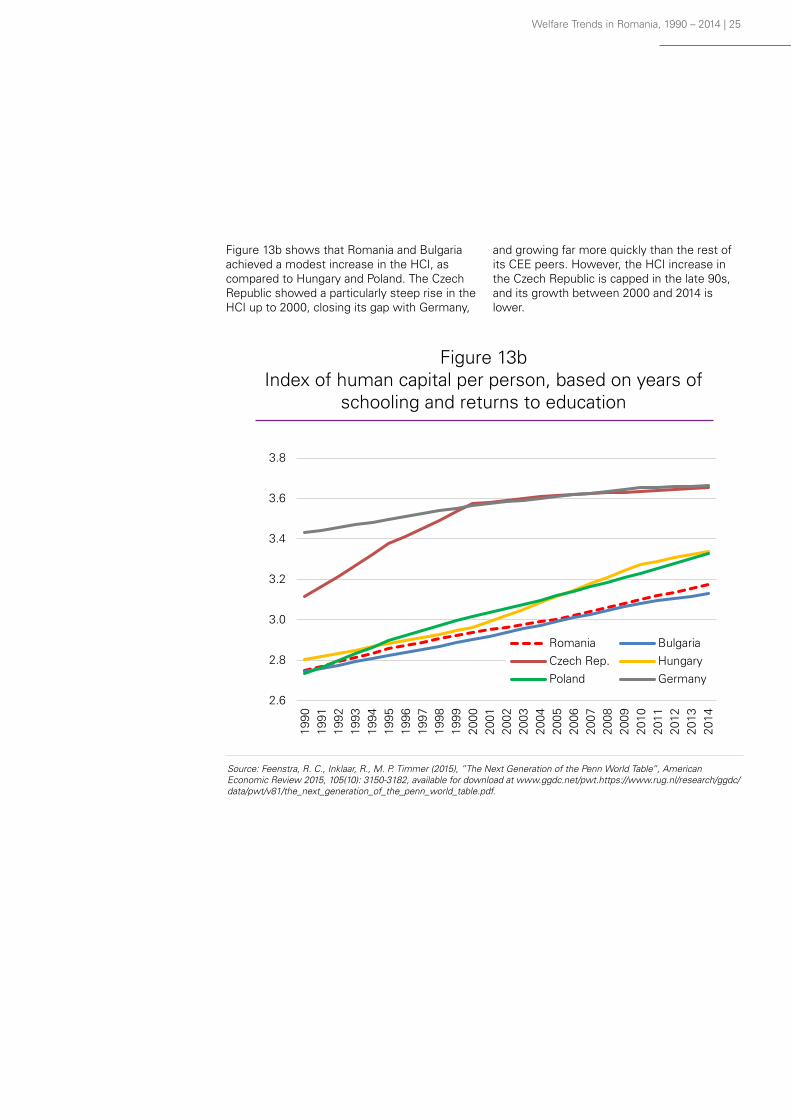
Welfare Trends in Romania, 1990 – 2014 | 25
Figure 13b shows that Romania and Bulgaria achieved a modest increase in the HCI, as compared to Hungary and Poland. The Czech Republic showed a particularly steep rise in the HCI up to 2000, closing its gap with Germany,
and growing far more quickly than the rest of its CEE peers. However, the HCI increase in the Czech Republic is capped in the late 90s, and its growth between 2000 and 2014 is lower.
Figure 13bIndex of human capital per person, based on years of
schooling and returns to education
Source: Feenstra, R. C., Inklaar, R., M. P. Timmer (2015), ”The Next Generation of the Penn World Table”, American Economic Review 2015, 105(10): 3150-3182, available for download at www.ggdc.net/pwt.https://www.rug.nl/research/ggdc/data/pwt/v81/the_next_generation_of_the_penn_world_table.pdf.
19
The second half of the 2000s brought a glut of tertiary students for most of the CEE countries. The potential causes are multiple and country-specific. In Romania, for example, the country with the steepest contraction in the rate of university enrolment, the increasing difficulty of the baccalaureate significantly reduced the number of candidates for admission to universities. But above all, interest in the qualifications offered by universities declined, primarily because of a mismatch between the latter and the demands of the labour market, which led to difficulties in graduates finding appropriate jobs. Another reason is the low salaries offered by employers, which were disproportionate with the level of training. Salaries were also affected by the recession subsequent to the financial crisis. As a result, more young people either turned to a less qualified job, or decided to emigrate - to study or to achieve a decent income. For these reasons, between 2007 and 2013, the number of students in Romania has halved, as a report of the Court of Accounts23found. Romania's exceptional development until 2009 should be viewed with reservations, because it says nothing about the quality of education and hence about its usefulness both for personal development, and for contributing to increasing revenues. The latter is taken into account by the human capital index (HCI), conducted by PWT. The HCI estimation is based on the number of years of schooling and its marginal rate of return. Figure 13b shows that Romania and Bulgaria achieved a modest increase in the HCI, as compared to Hungary and Poland. The Czech Republic showed a particularly steep rise in the HCI up to 2000, closing its gap with Germany, and growing far more quickly than the rest of its CEE peers, in absolute values. In relative terms, though, because the HCI increase in the Czech Republic is capped in the late 90s, its growth between 2000 and 2014 is lower.
Figure 13b
Source: Penn World Table 9.0.
4.3. The big picture 4.3.1. Welfare development relative scores After going through a significant amount of statistical analysis and explanations it is time to synthesize 23Curtea de Conturi a României (2015) – Analiza fundamentării şi evoluţiei situaţiei obiectivului privind creşterea procentului absolvenţilor de învăţământ superior, în conformitate cu prevederile Strategiei Europa 2020, pp. 36 – 37, http://www.curteadeconturi.ro/Publicatii/SINTEZAAPInvsup.pdf.
2.6
2.8
3.0
3.2
3.4
3.6
3.8
1990
1991
1992
1993
1994
1995
1996
1997
1998
1999
2000
2001
2002
2003
2004
2005
2006
2007
2008
2009
2010
2011
2012
2013
2014
Romania BulgariaCzech Rep. HungaryPoland Germany
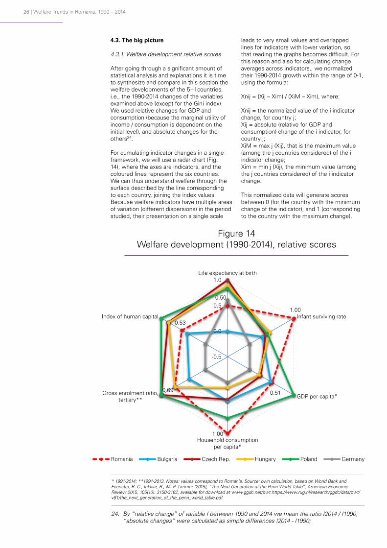
26 | Welfare Trends in Romania, 1990 – 2014
4.3. The big picture
4.3.1. Welfare development relative scores
After going through a significant amount of statistical analysis and explanations it is time to synthesize and compare in this section the welfare developments of the 5+1countries, i.e., the 1990-2014 changes of the variables examined above (except for the Gini index). We used relative changes for GDP and consumption (because the marginal utility of income / consumption is dependent on the initial level), and absolute changes for the others24.
For cumulating indicator changes in a single framework, we will use a radar chart (Fig. 14), where the axes are indicators, and the coloured lines represent the six countries. We can thus understand welfare through the surface described by the line corresponding to each country, joining the index values. Because welfare indicators have multiple areas of variation (different dispersions) in the period studied, their presentation on a single scale
leads to very small values and overlapped lines for indicators with lower variation, so that reading the graphs becomes difficult. For this reason and also for calculating change averages across indicators,, we normalized their 1990-2014 growth within the range of 0-1, using the formula:
Xnij = (Xij – Xim) / (XiM – Xim), where:
Xnij = the normalized value of the i indicator change, for country j;Xij = absolute (relative for GDP and consumption) change of the i indicator, for country j;XiM = max j (Xij), that is the maximum value (among the j countries considered) of the i indicator change;Xim = min j (Xij), the minimum value (among the j countries considered) of the i indicator change.
This normalized data will generate scores between 0 (for the country with the minimum change of the indicator), and 1 (corresponding to the country with the maximum change).
Figure 14Welfare development (1990-2014), relative scores
* 1991-2014; **1991-2013. Notes: values correspond to Romania. Source: own calculation, based on World Bank and Feenstra, R. C., Inklaar, R., M. P. Timmer (2015), ”The Next Generation of the Penn World Table”, American Economic Review 2015, 105(10): 3150-3182, available for download at www.ggdc.net/pwt.https://www.rug.nl/research/ggdc/data/pwt/v81/the_next_generation_of_the_penn_world_table.pdf.
20
of the variables examined above (except for the Gini index). We used relative changes for GDP and consumption (because the marginal utility of income / consumption is dependent on the initial level), and absolute changes for the others24. For cumulating indicator changes in a single framework, we will use a radar chart (Fig. 15), where the axes are indicators, and the coloured lines represent the six countries. We can thus understand welfare through the surface described by the line corresponding to each country, joining the index values. Because welfare indicators have multiple areas of variation (different dispersions) in the period studied, their presentation on a single scale leads to very small values and overlapped lines for indicators with lower variation, so that reading the graphs becomes difficult. For this reason, we normalized their 1990-2014growth within the range of 0-1 (Fig. 14), using the formula:
Xnij = (Xij – Xim) / (XiM – Xim), where:
Xnij = the normalized value of the i indicator change, for country j; Xij = absolute (relative for GDP and consumption) change of the i indicator, for country j; XiM = max j (Xij), that is the maximum value (among the j countries considered) of the i indicator change; Xim = min j (Xij), the minimum value (among the j countries considered) of the i indicator change. This normalized data will generate scores between 0 (for the country with the minimum change of the indicator), and 1 (corresponding to the country with the maximum change).
Figure 14
* 1991-2014; **1991-2013. Notes: red values correspond to Romania. Source: own calculation, based on World Bank and Penn World Table 9.0 data.
24 By “relative change” of variable I between 1990 and 2014 we mean the ratio I2014 / I1990; “absolute changes” were calculated as simple differences I2014 - I1990.
0.50
1.00
0.51
1.00
0.69
0.53
-0.5
0.0
0.5
1.0Life expectancy at birth
Infant surviving rate
GDP per capita*
Household consumptionper capita*
Gross enrolment ratio,tertiary**
Index of human capital
Welfare development (1990-2014), relative scores
Romania Bulgaria Czech Rep. Hungary Poland Germany
24. By “relative change” of variable I between 1990 and 2014 we mean the ratio I2014 / I1990; “absolute changes” were calculated as simple differences I2014 - I1990;

Welfare Trends in Romania, 1990 – 2014 | 27
Figure 14 reveals that, although Romania has benefitted from consistent welfare development, it ranks first for only two of the six indicators: infant survival rate and household consumption. The GDP change is second after Poland, whose growth performance is higher than all the other countries. For the tertiary enrolment ratio, Romania is only in third position because the initial steep growth in 2000-2009 was offset by the subsequent dramatic decrease in the number of students (Figure 13a). Even less favourable positions resulted for life expectancy and HCI (fifth and fourth place, respectively). For life expectancy, Romania’s and Bulgaria’s initial downward trend (1990-1997) is the main reason for their late start and low overall changes.
In Annex 2 we presented the total average relative scores of welfare development for each country, calculated as arithmetic means of the average scores corresponding to each of the three welfare pillars: health, income and consumption, and education. In their turn, these were calculated as arithmetic means of the two indicator changes included in each pillar. Poland’s development ranks first for two pillar averages (income and consumption, and education) and also as regards overall welfare growth between 1990 and 2014 (with a total average score of 0.82). Romania’s development ranks first in health, second in income and consumption, and fourth in education, while its total average score is 0.70. A representation in graph form of the total average score for each country presents a suggestive summary of the above analysis:
Germany’s last place might be evidence of the welfare convergence between Eastern and Western Europe. However, this is not necessarily true in the case of GDP and private consumption, because lower relative changes for Germany could mean higher absolute changes, when the base level is
sufficiently higher. This issue is also relevant when questioning the closing of the gap between Romania and the other countries, as regards GDP and consumption. This is why the following section will deal precisely with the absolute gaps.
Figure 15Welfare development (1990-2014*), total relative scores
* 1991-2014 for GDP per capita and household consumption per capita, 1991-2013 for tertiary enrolment rate. Source: own calculation, based on World Bank and Feenstra, R. C., Inklaar, R., M. P. Timmer (2015), ”The Next Generation of the Penn World Table”, American Economic Review 2015, 105(10): 3150-3182, available for download at www.ggdc.net/pwt.https://www.rug.nl/research/ggdc/data/pwt/v81/the_next_generation_of_the_penn_world_table.pdf.
21
Figure 14 reveals that, although Romania has benefitted from consistent welfare development, it ranks first for only two of the six indicators: infant survival rate and household consumption. The GDP change is second after Poland, whose net growth performance is higher than all the other countries. For the tertiary enrolment ratio, Romania is only in third position because the initial steep growth in 2000-2009 was offset by the subsequent dramatic decrease in the number of students (Figure 13a). Less favourable positions resulted for life expectancy and HCI (fifth and fourth place, respectively). For life expectancy, Romania’s and Bulgaria’s initial downward trend (1990-1997) is the main reason for their late start and low overall changes. In Annex 2 we presented the total average relative scores of welfare development for each country, calculated as arithmetic means of the average scores corresponding to each of the three welfare pillars: health, income and consumption, and education. In their turn, these were calculated as arithmetic means of the two indicators included in each pillar. Poland’s development ranks first for two pillar averages (income and consumption, and education) and also as regards overall welfare growth between 1990 and 2014 (with a total average score of 0.82). Romania’s development ranks first in health, second in income and consumption, and fourth in education, while its total average score is 0.70. A representation in graph form of the total average score for each country presents a suggestive summary of the above analysis:
Figure 15
* 1991-2014 for GDP per capita and household consumption per capita, 1991-2013 for tertiary enrolment rate. Source: own calculation, based on World Bank and Penn World Table 9.0. Germany’s last place might be evidence of the welfare convergence between Eastern and Western Europe. However, this is not necessarily true in the case of GDP and private consumption, because lower relative changes for Germany could mean higher absolute changes, when the base level is sufficiently higher. This issue is also relevant when questioning the closing of the gap between Romania and the other countries, as regards GDP and consumption. This is why the following section will deal precisely with the absolute gaps. 4.3.1. Welfare absolute gaps developments To clarify in-depth the development of disparities between Romania and the other countries, in Figure 16 we have presented these gaps, for each indicator, in absolute figures25, corresponding to the start and the end year of the period under survey (1990 and 201426). We notice that for GDP and consumption, the results are not entirely predicted by Figure 14. For instance, although the GDP relative change in Romania is higher than that in Germany and the Czech Republic, the respective absolute gaps increased. 25 Absolute gaps (monetary units) for indicator I were calculated as simple differences I Romania – I j, where j represents the other five countries considered. 261991 and 2014 for GDP per capita and consumption per capita, 1991 and 2013 for tertiary enrolment rate.
0.000
0.100
0.200
0.300
0.400
0.500
0.600
0.700
0.800
0.900
Germany Bulgaria Hungary Czech Rep. Romania Poland
0.101
0.318
0.529
0.6290.704
0.822

28 | Welfare Trends in Romania, 1990 – 2014
4.3.2 Welfare absolute gaps developments
To clarify in-depth the development of disparities between Romania and the other countries, in Figure 16 we have presented these gaps, for each indicator, in absolute figures25, corresponding to the start and the end year of the period under survey (1990 and 201426). We notice that for GDP and consumption, the results are not entirely predicted by Figure 14. For instance, although the GDP relative change in Romania is
higher than that in Germany and the Czech Republic, the respective absolute gaps increased. The same applies when considering the gap between Romania and Poland in terms of household consumption. These findings confirm that relative changes can be misleading when estimating gap trends. For the rest of the indicators, as expected, the findings in Figure 16 correspond to those in Figure 14, i.e., higher absolute changes for Romania led to a narrowing of the gaps, and the reverse.
26. 1991 and 2014 for GDP per capita and consumption per capita, 1991 and 2013 for tertiary enrolment rate.
Figure 16Welfare absolute gaps between Romania and the other
considered countries
Note: Negative gaps mean lower values for Romania, relative to the other countries considered; positive gaps mean higher values.Source: own calculations, based on World Bank Indicators and Feenstra, R. C., Inklaar, R., M. P. Timmer (2015), ”The Next Generation of the Penn World Table”, American Economic Review 2015, 105(10): 3150-3182, available for download at www.ggdc.net/pwt.https://www.rug.nl/research/ggdc/data/pwt/v81/the_next_generation_of_the_penn_world_table.pdf.
22
the end year of the period under survey (1990 and 201426). We notice that for GDP and consumption, the results are not entirely predicted by Figure 14. For instance, although the GDP relative change in Romania is higher than that in Germany and the Czech Republic, the respective absolute gaps increased. The same applies when considering the gap between Romania and Poland in terms of household consumption. These findings confirm that relative changes can be misleading when estimating gap trends. For the rest of the indicators, as expected, the findings in Figure 16 correspond to those in Figure 14, i.e., higher absolute changes for Romania led to a narrowing of the gaps, and the reverse.
Figure 16 Welfare absolute gaps between Romania and the other considered countries
Special attention is required when considering the change in the economic disparity between Romania and Germany, because it can be considered an illustration of the convergence trend with the highly developed countries from Western Europe (Germany is considered “the engine of Europe”27). Consequently, Figure 17 details how gaps in GDP and consumption have evolved over time, both in 261991 and 2014 for GDP per capita and consumption per capita, 1991 and 2013 for tertiary enrolment rate. 27 http://www.economist.com/node/15663362.
-6 -4 -2 0 2
Bulgaria
Czech Rep.
Hungary
Poland
GermanyGap
bet
wee
n R
oman
ia a
nd:
Life expectancy at birth, years
20141990
-25 -20 -15 -10 -5 0
Bulgaria
Czech Rep.
Hungary
Poland
Germany
Gap
bet
wee
n R
oman
i and
:
Infant survival rate, ‰
20141990
-25,000 -15,000 -5,000 5,000
Bulgaria
Czech Rep.
Hungary
Poland
Germany
Gap
bet
wee
n R
oman
ia a
nd:
GDP per capita, 2011 USD PPP
20141991
-15,000 -10,000 -5,000 0 5,000
Bulgaria
Czech Rep.
Hungary
Poland
Germany
Gap
bet
wee
n R
oman
ia a
nd:
Household consumption per capita, 2011 USD PPP
20141991
-30 -20 -10 0
Bulgaria
Czech Rep.
Hungary
Poland
GermanyGap
bet
wee
n R
oman
ia a
nd:
Gross enrolment ratio, tertiary, p.p.
2013
1991
-0.8 -0.6 -0.4 -0.2 0.0 0.2
Bulgaria
Czech Rep.
Hungary
Poland
GermanyGap
bet
wee
n R
oman
ia a
nd:
Human capital per person, index
20141990
25. Absolute gaps for indicator I were calculated as simple differences I Romania – I j, where j represents the other five countries considered.

Welfare Trends in Romania, 1990 – 2014 | 29
Special attention is required when considering the change in the economic disparity between Romania and Germany, because it can be considered an illustration of the convergence trend with the highly developed countries from Western Europe (Germany is considered “the engine of Europe”27).
Consequently, Figure 17 details how gaps in GDP and private consumption have evolved over time, both in absolute and relative terms (percentage)28.
One may distinguish three principal sub-periods. The early one (1990-2000) corresponds to the first decade of transition to the market economy in the CEE countries, associated with a decline in economic
performance, and gap widening. The second step (2000-2008) involved sustained economic growth in CEE, hence a tendency towards a narrowing of the gap compared to Western Europe. In the GDP case, the absolute gap also continued to decrease in 2009, due to Germany’s large GDP contraction in that year. During the last stage (2008-2014), we witness again a slight widening of gaps. This tendency was initially driven by the quick GDP recovery in Germany after the 2008-2009 instability, while in Romania the period of convalescence lasted longer. Nevertheless, during the last two years Romania has struggled to catch up, and there might be prerequisites for resuming the tendency towards closing the gaps in the next few years.
27. http://www.economist.com/node/15663362.28. Relative gap (%) for indicator I is the ratio (It Romania – It Germany) / It Germany, where It is
the value of indicator I in year t.
Figure 17GDP and household consumption, gap between
Romania and Germany
23
Consequently, Figure 17 details how gaps in GDP and consumption have evolved over time, both in absolute and relative terms (percentage) 28. One may distinguish three principal sub-periods. The early one (1990-2000) corresponds to the first decade of transition to the market economy in the CEE countries, associated with a decline in economic performance, and gap widening. The second step (2000-2008) involved sustained economic growth in CEE, hence a tendency towards a narrowing of the gap compared to Western Europe. In the GDP case, the absolute gap also continued to decrease in 2009, due to Germany’s large GDP contraction in that year. During the last stage (2008-2014), we witness again a slight widening of gaps. This tendency was initially driven by the quick GDP recovery in Germany after the 2008-2009 instability, while in Romania the period of convalescence lasted longer. Nevertheless, during the last two years Romania has struggled to catch up, and there might be prerequisites for resuming the tendency towards closing the gaps in the next few years. In 2014, the relative gap for both GDP and private consumption was around 56%, which means that the levels of these indicators in Romania represented around 44% of the respective indicators in Germany.
Figure 17
Note: A negative gap (either absolute or relative) means a lower value for Romania, relative to Germany (see footnotes 25 and 27 for details). Source: own calculations, based on World Bank Indicators. 5. Final remarks Summarizing the above results, we can conclude that 1990-2014 welfare development in Romania, determined using the indicators and methodology already presented, appears to have been consistent and robust. If we look at the overall welfare development relative scores, Romania ranks 2nd among the six countries under survey, after Poland. Accordingly, even though Romania used to be below other CEE countries in absolute figures, the positive developments we have observed for some indicators have the potential to lead to convergence with countries better positioned so far, as confirmed by reducing gaps for these indicators. However, this 2nd rank comprises mixed performances among the analysed indicators. For instance, Romania’s wellbeing development lags behind some other CEE countries for life expectancy, tertiary enrolment and human capital. As a result, absolute gaps have expanded. Moreover, in the case of GDP, although its relative growth was lower only than that of Poland, the absolute gap between Romania and other two countries (Czech Republic and Germany) widened in 2014, as compared with 1991. 28 Relative gap (%) for indicator I is the ratio (It Romania – It Germany) / It Germany, where It is the value of indicator I in year t.
-90
-80
-70
-60
-50
-40
-30
-20
-10
0
-30,000
-25,000
-20,000
-15,000
-10,000
-5,000
0
1990
1991
1992
1993
1994
1995
1996
1997
1998
1999
2000
2001
2002
2003
2004
2005
2006
2007
2008
2009
2010
2011
2012
2013
2014
perc
enta
ge
2011
USD
PPP
GDP and household consumption,gap between Romania and Germany
GDP per capita, absolute gap (left scale)Household consumption per capita, absolute gap (left scale)GDP per capita, relative gap (right scale)Household consumption per capita, relative gap (right scale)
Note: A negative gap (either absolute or relative) means a lower value for Romania, relative to Germany (see footnotes 25 and 28 for details). Source: own calculations, based on World Bank Indicators.

30 | Welfare Trends in Romania, 1990 – 2014
Summarizing the above results, we can conclude that 1990-2014 welfare development in Romania, determined using the indicators and methodology already presented, appears to have been consistent and robust. If we look at the overall welfare development relative scores, Romania ranks 2nd among the six countries under survey, after Poland. Accordingly, even though Romania used to be below other CEE countries in absolute figures, the positive developments we have observed for some indicators show a convergence tendency with countries better positioned so far, as confirmed by reducing gaps for these indicators.
However, this 2nd rank comprises mixed performances among the analysed indicators. For instance, Romania’s wellbeing development lags behind some other CEE countries for life expectancy, tertiary enrolment and human capital. As a result, absolute gaps have expanded. Moreover, in the case of GDP, although its relative growth was lower only than that of Poland, the absolute gap between Romania and other two countries (Czech Republic and Germany) widened in 2014, as compared with 1991.
We have seen that the wellbeing progress of Romania and other CEE countries is higher than Germany’s, for most of the indicators (except for life expectancy). This could suggest a convergence trend between Eastern and Western Europe, as far as Germany’s development is representative for the dynamics in Western European countries. However, this may not be true for GDP and consumption (for which we calculated relative changes), as exemplified above with the case of Romania.
The above clearly points at a few development directions which should be followed by economic and social policy makers in Romania. As such, important sectors such as healthcare and education require significant attention both in terms of financial investment and operational efficiency.
Even though Romania used to be below other CEE countries in absolute figures, the positive developments we have observed for some indicators indicate a convergence tendency with countries better positioned so far, as confirmed by reducing gaps for these indicators.
“
5. Final remarks

Welfare Trends in Romania, 1990 – 2014 | 31
Limitations of our research
We need to stress at this point that the statistical indicators available for the entire period proposed in this research are limited, especially for CEE countries, and this shortcoming may have not allowed us to choose the most significant variables for each aspect of welfare. As we consider our present endeavour a starting point for a possible future series of research papers, we consider that income, consumption and wealth are the main issues that should be further analysed in relation to the objective wellbeing topic. Their study at household level and not at national level is preferable when studying welfare. In terms of household income, the analysis of disposable income, which excludes taxes paid, is the most appropriate. In the case of consumption, an important methodological step would be its segmentation into different categories of goods and services.
On the other hand, further research on household income (and other aspects of wellbeing) inequality, using various methodologies, is strongly recommended. Assessing distribution of individuals / households by income level is also advisable, to detect possible tendencies of
polarisation. Another relevant aspect of welfare is the wealth of the population - financial and non-financial assets - and also the balance sheet situation, i.e., the relationship between assets, liabilities and disposable income. All these measures have only recently begun to be quantified and included in statistical databases and hence they were not included in our long-term analysis. The compromise between timing and depth of research cannot be avoided, both for welfare and many other economic and social issues. As a result, future short-term in-depth investigations to deepen our understanding of various aspects of welfare may contribute to completing the big picture.
Given the results obtained in this paper, it could prove useful to research the subjective coordinate of wellbeing in Romania. This would involve a totally different approach and methodology, as already presented in the introductory section. Beside the implicit added value of such an analysis, it would also be interesting to benchmark the relevant results against those obtained by deploying statistical indicators, i.e. the objective analysis. We leave this chapter open for the future.

32 | Welfare Trends in Romania, 1990 – 2014
1. Axenciuc, V. (2012), “Produsul intern brut al României 1862-2000. Serii statistice secular și argumente metodologice, volumul I: Produsul intern brut 1862-2000. Sinteza seriilor de timp a indicatorilor globali, pe secțiuni temporale”, EdituraEconomică, București;
2. Curtea de Conturi a României (2015), “Analiza fundamentării şi evoluţiei situaţiei obiectivului privind creşterea procentului absolvenţilor de învăţământ superior, în conformitate cu prevederile Strategiei Europa 2020”;
3. Conceição, P., & Bandura, R. (2008), “Measuring subjective wellbeing: A summary review of the literature”, United Nations Development Programme (UNDP) Development Studies, Working Paper;
4. Easterlin, R. A. (1974), “Does economic growth improve the human lot? Some empirical evidence”, Nations and households in economic growth, 89, 89-125;
5. Easterlin, R. A. (1995), “Will raising the incomes of all increase the happiness of all?”, Journal of Economic Behavior & Organization, 27(1), 35-47;
6. EU Commission (2009), GDP and beyond: measuring progress in a changing world, COM (2009) 433;
7. Feenstra, R. C., Inklaar, R., M. P. Timmer (2016), What is new in PWT 9.0?,Groningen Growth and Development Centre, University of Groningen;
8. Feenstra, R. C., Inklaar, R., M. P. Timmer (2015a), ”The Next Generation of the Penn World Table”, American Economic Review 2015, 105(10): 3150-3182, available for download at www.ggdc.net/pwt.https://www.rug.nl/research/ggdc/data/pwt/v81/the_next_generation_of_the_penn_world_table.pdf;
9. Feenstra, R. C., Inklaar, R., M. P. Timmer (2015b), Human capital in PWT 9.0, Groningen Growth and Development Centre, University of Groningen;
10. Frey, B. S., & Stutzer, A. (2002), Happiness and Economics: How the Economy and Iinstitutions Affect Well-Being, Princeton and Oxford: Princeton University Press;
11. Helliwell, J. F., R. Layard, and J. Sachs, eds. (2016), World Happiness Report 2016 Update (Vol.I), New York, Sustainable Development Solutions Network;
12. Inklaar, R., M. P. Timmer (2013) – Capital, labour and TFP in PWT8.0,Groningen Growth and Development Centre, University of Groningen;
13. Legatum Institute (2016), The Legatum Prosperity Index 2016. Bringing prosperity to life, Tenth Edition 2007-206, London;
14. New Economics Foundation (2016), The Happy Planet Index 2016. A global index of sustainable wellbeing;
15. Stiglitz, J. E., A. Sen, and J. P. Fitoussi (2010), Report by the Commission on the measurement of economic performance and social progress: Commission on the Measurement of Economic Performance and Social Progress, Paris;
16. United Nations Development Programme (2015), Human Development Report 2015.Work for Human Development, New York;
17. Weimann, J., A. Knabe, and R. Schöb (2015), Measuring happiness: The economics of well-being, MIT Press.
Bibliography

Welfare Trends in Romania, 1990 – 2014 | 33
Indicator Unit Period Data sources
Health
• Life expectancy at birth, total• Infant survival rate, per 1,000 live
births
years‰
1990 - 20141990 - 2014
• World Bank Indicators (updated 17.11.16)• Based on World Bank Indicators: Mortality
rate, infant per 1,000 live births (updated 17.11.16)
Income
• Gross domestic product, per capita, in Romania
• Gross domestic product, per capita• Gross national income, % of GDP
• Gini index, World Bank estimate
2000 USD PPP
2011 USD PPP%
%
1950 - 2015
1990 – 20141990– 2014
1989 - 2012
• Axenciuc (2012), and authors’ calculations based on Axenciuc (2012) and Eurostat: Gross domestic product chained linked volumes, Index 2010=100, per capita (updated 03.11.16)
• World Bank Indicators (updated 17.11.16)• Based on World Bank Indicators: GDP, current
LCU; GNI, current LCU (updated 17.11.16)• World Bank Indicators (updated 17.11.16)
Consumption
• Household final consumption ex-penditure per capita
2011 USD PPP 1990 - 2014 • Based on World Bank Indicators: Household final consumption expenditure per capita, constant 2010 US$; Official exchange rate, LCU per US$, period average; Consumer price index, 2010=100; PPP conversion factor, private consumption, LCU per international $ (updated 17.11.16)
Education
• Gross enrolment ratio, tertiary, both sexes
• Index of human capital per person, based on years of schooling and returns to education
%
index
1990 - 2014
1990 - 2014
• World Bank Indicators (updated 17.11.16)
• Feenstra, R. C., Inklaar, R., M. P. Timmer (2015), ”The Next Generation of the Penn World Table”, American Economic Review 2015, 105(10): 3150-3182, available for download at www.ggdc.net/pwt.https://www.rug.nl/research/ggdc/data/pwt/v81/the_next_generation_of_the_penn_world_table.pdf.(extracted 20.11.16)
Appendix 1
Indicators, measurement units, periods
under survey, and data sources
Source: own compilation.

34 | Welfare Trends in Romania, 1990 – 2014
Indicator
\
Country
1. Health 2. Income & Consumption 3. Education Total average
Life expectancy
at birth
Infant survival
rate
Health average
GDP per
capita *
Household consumption per capita *
Income & Consumption
average
Gross enrolment
ratio, tertiary **
Index of human capital
Education average
Romania 0.498 1.000 0.749 0.508 1.000 0.754 0.687 0.531 0.609 0.704
Bulgaria 0.000 0.287 0.143 0.474 0.367 0.420 0.366 0.414 0.390 0.318
Czech Rep. 1.000 0.351 0.675 0.249 0.335 0.292 0.996 0.845 0.920 0.629
Hungary 0.893 0.456 0.675 0.211 0.100 0.156 0.685 0.830 0.758 0.529
Poland 0.831 0.398 0.614 1.000 0.701 0.850 1.000 1.000 1.000 0.822
Germany 0.608 0.000 0.304 0.000 0.000 0.000 0.000 0.000 0.000 0.101
Appendix 2
Welfare development (1990-2014)
relative scores
* 1991-2014; **1991 – 2013. Source: own calculations, based on World Bank Indicators and Feenstra, R. C., Inklaar, R., M. P. Timmer (2015), ”The Next Generation of the Penn World Table”, American Economic Review 2015, 105(10): 3150-3182, available for download at www.ggdc.net/pwt.https://www.rug.nl/research/ggdc/data/pwt/v81/the_next_generation_of_the_penn_world_table.pdf.


The information contained herein is of a general nature and is not intended to address the circumstances of any particular individual or entity. Although we endeavor to provide accurate and timely information, there can be no guarantee that such information is accurate as of the date it is received or that it will continue to be accurate in the future. No one should act on such information without appropriate professional advice after a thorough examination of the particular situation.The KPMG name and logo are registered trademarks or trademarks of KPMG International. © 2017 KPMG Romania S.R.L., a Romanian limited liability company and a member firm of the KPMG network of independent member firms affiliated with KPMG International Cooperative (“KPMG International”), a Swiss entity. All rights reserved. Printed in Romania.