Welfare Reform and Indirect Impacts on Health

Marianne P. Bitler University of California-Irvine and NBER

mbitler@uci.edu

and

Hilary W. Hoynes University of California, Davis and NBER

hwhoynes@ucdavis.edu

March 14, 2007 First draft: January 30, 2006

This paper was prepared for the conference “Health Effects of Non-Health Policy” held in Washington, DC on February 9–10, 2006. The data used herein are derived from data files made available to researchers by the Manpower Demonstration Research Corporation (MDRC) and Mathematica Policy Research (MPR). We thank MDRC and MPR for assistance with the public use data. The authors remain solely responsible for how the data are used or interpreted. We thank Becky Blank, Jim House, George Kaplan, Harold Pollack, Narayan Sastry, Bob Schoeni, Neeraj Sood and conference participants for helpful comments, and Peter Huckfeldt for excellent research assistance.

1

I. Introduction

Beginning in the early 1990s, many states used waivers to reform their Aid to Families with

Dependent Children (AFDC) programs. This state experimentation resulted in landmark legislation

which in 1996 eliminated AFDC and replaced it with Temporary Assistance for Needy Families (TANF).

TANF—like the earlier AFDC program—provides cash grants to low income families with children and

is a key element of the nation’s economic safety net. The roots of this reform lie in long time concern that

AFDC led to reductions in work, decreases in marriage, and increases in nonmarital births among low

income women.

These important policy changes, known collectively as welfare reform, were implemented with a

desire to increase work among low skilled single parent families, reduce dependency on welfare, reduce

births outside marriage, and increase the formation of two parent families. In the wake of welfare reform,

between 1990 and 2000 welfare caseloads declined by 50 percent (U.S. Department of Health and Human

Services, 2007) and the employment rate of low skilled single parents with children increased by 13

percentage points, from 74 percent to 87 percent (Eissa and Hoynes 2006). An enormous literature has

developed which evaluates the impact of welfare reform on caseloads and labor supply, as well as

income, poverty, fertility, marriage, and family and child wellbeing.1

Importantly, these goals of welfare reform had little to do directly with health or health insurance.

Despite this lack of direct connection to health, however, we argue that welfare reform may have

important indirect impacts on health. In this chapter, we summarize what is known about the impacts of

welfare reform on health insurance, health care utilization, and health status. Understanding if and how

welfare reform impacts health is extremely important given the pre-existing inverse relationship between

income and health. Welfare recipients are worse off than the general population. This both complicates

the task of deciphering the effects of welfare reform and makes possible negative health impacts of

welfare a topic of extra concern. For example, Kaplan et al. (2005) show that current and former welfare

recipients are more likely to smoke, be obese, have higher rates of hypertension, diabetes, and elevated

2

glycosylated hemoglobin levels, and have worse self reported health status compared to other women of

the same age and race.

We begin, in the next section, with a description of the key policy changes over this period. The

central changes in the TANF program include lifetime time limits for receiving cash assistance, work

requirements, financial sanctions, and enhanced earnings disregards.2 We also discuss the concurrent

changes in public health insurance for poor families through the expansions of Medicaid and introduction

of the State Children’s Health Insurance Program (SCHIP).

In section III, we outline the pathways by which welfare reform may affect health-related

outcomes. One pathway is through health insurance—reform leads to reductions in welfare participation

which is expected to reduce health insurance coverage (employer-provided coverage may increase but by

less than Medicaid coverage declines). The other pathways are more indirect—for example welfare

reform may impact families’ economic resources, time endowment, and levels of stress which may then

affect health care utilization and health status.

The early studies on this issue documented very low rates of health insurance coverage following

federal reform. For example, Bowen Garrett and John Holahan (2000) found that one year after leaving

welfare, one-half of women and almost one-third of children are uninsured.3 This “leaver” analysis

provides an important profile of the well-being of families departing the welfare rolls. However, an

analysis of welfare leavers is largely descriptive and not adequate for identifying the impact of welfare

reform. This important identification issue is assessed more fully in section IV where we discuss the

methods that have been used to estimate impacts of welfare reform.

In section V, we provide a comprehensive review of the literature on the impacts of welfare

reform on health. The literature includes nonexperimental estimates (typically state-panel models using

variation in the timing and presence of reform across states) and experimental estimates (randomized

experimental evaluations of state waiver programs). These two approaches have important and distinct

advantages and disadvantages. Nonexperimental (or observational) studies have the advantage of

measuring impacts on the overall population, but are subject to concerns about identification due to

3

sample selection and endogenous policies. Experimental studies have the advantage of randomization but

the results apply to the experimental context—typically one state, one set of policies, and one group of

welfare recipients. Overall, our review of the literature shows that welfare reform lead to reduction in

health insurance coverage with small and often insignificant impacts on health care utilization and health

status. Some studies find evidence of a modest decrease in utilization and small changes in health

behaviors. They suggest that welfare-to-work programs need not have large negative health effects.

In section VI, we augment the literature review with an analysis of data from separate state

welfare reform experiments in Connecticut, Iowa, Florida, Minnesota, and Vermont. Each of these states

represents reforms prior to TANF, but as discussed more fully below, all randomized experimental

evaluation of welfare reform were of state waivers while there were no evaluations of TANF. We present

estimates of the impact of reform on health insurance, health utilization (child doctor or dentist visits,

whether the child has a place to go for routine care) and health status (parent rated child’s health status,

whether the case head is at risk for depression, and whether the focal child scores poorly on a Behavioral

Problem Index). These five states were chosen because their experimental evaluations provided the most

comprehensive data on health and their welfare reform policies were the most similar to the eventual

federal TANF policies. It is important to note, however, that our results reflect the specific policies that

were implemented by these states and do not necessarily reflect “average” TANF policies. With that

caveat, our analysis of these five states finds that reform led to small changes in health insurance

coverage, mixed evidence on health care utilization, and suggestive evidence of improvements in child

health status for children two to nine at the beginning of the experiments.

An important drawback of this chapter and indeed much of the existing literature on welfare

reform and health is that most of the available data is quite limited. The experimental literature, while

able to avoid issues of selection bias common to observational studies, is restricted to looking at health

outcomes about which information was collected during surveys administered to participants. These

surveys tended to ask about health insurance coverage in some detail, and a number also collected

information about the outcomes we present here. Yet the experimental surveys did not collect data on

4

many important health outcomes of interest such as whether the children are suffering from

developmental delays, asthma, or chronic ear conditions, or are obese or overweight; whether recipients

are overweight or obese; whether recipients suffer from substance abuse or sexually transmitted diseases,

have negative health behaviors such as smoking, or have chronic conditions such as asthma, hypertension,

or diabetes. A number of health surveys (which could be used for nonexperimental analyses) do collect

information on these outcomes and/or others of interest, but either do not contain information allowing

one to identify whether women are in a group likely to be affected by reform, do not contain information

for a consistent panel of states and years spanning reform, or do not have large enough samples to

plausibly identify the effects of reform. Consequently, we are left with the outcomes we and the previous

literature have focused on.

II. Welfare Reform in the 1990s

Beginning in the early 1990s, many states were granted waivers to make changes to their AFDC

programs. About half of the states implemented some sort of welfare waiver between 1993 and 1995

(Office of the Assistant Secretary for Planning and Evaluation, DHHS, 2001). Following this period of

state experimentation, PRWORA was enacted in 1996, replacing AFDC with TANF. PRWORA

originally indicated that all states had to have their TANF programs in place and have implemented

TANF by July 1, 1997, although subsequently this deadline was relaxed (Administration of Children and

Families, DHHS, 2002). All states implemented PRWORA in a seventeen month period between

September 1996 and January 1998 (Gil Crouse, 1999; Administration for Children and Families, DHHS,

1997).

The main goals of welfare reform are to increase work, reduce dependency on welfare, reduce

births outside marriage, and to increase the formation of two parent families. While waiver and TANF

policies varied considerably across states, the reforms were generally welfare-tightening and pro-work.

More specifically, the welfare-tightening elements of reform include work requirements, financial

sanctions, time limits, family caps, and residency requirements.4 The loosening aspects of reform include

5

liberalized earnings disregards (which promote work by lowering the tax rate on earned income while on

welfare), increased asset limits, increased transitional Medicaid coverage, and expanded welfare

eligibility for two-parent families. Importantly, welfare reform—either the goals or resulting policies—

had little directly to do with health or health insurance.

During this period of welfare reform, however, other policies were expanding public health

insurance for low-income families. Historically, eligibility for Medicaid for the non-elderly and non-

disabled was tied directly to receipt of cash public assistance. In particular, the AFDC income eligibility

limits adopted by a state would also be used for Medicaid, and AFDC conferred automatic eligibility for

Medicaid. Thus, a family that received AFDC benefits would also be eligible for health insurance

through Medicaid. Conversely, if a family left AFDC, its members generally would lose Medicaid

coverage.5 However, in a series of federal legislative acts beginning in 1984, states were required to

expand Medicaid coverage for infants, children, and pregnant women beyond the AFDC income limits,

leading to large increases in eligibility (Jonathan Gruber 1997). These are known as the poverty-related

or OBRA Medicaid expansions. By 2001, these expansions mandated that all children in families with

income up to the Federal poverty limit were eligible for Medicaid, provided they met other requirements.

PRWORA further weakened the link between AFDC and Medicaid by requiring states to cover

any family that meets the pre-PRWORA AFDC income, resource, and family composition eligibility

guidelines (Ron Haskins 2001). This so-called 1931 program (named after the relevant section of the

Social Security Act, as amended by PRWORA) also allowed states to expand eligibility for parents

beyond the 1996 AFDC/Medicaid limits. Anna Aizer and Jeffrey Grogger (2003) report that by 2001,

about half the states had taken advantage of this program and expanded Medicaid access for parents

above the welfare income cutoffs.

In addition to the time limits, work requirements and sanctions, PRWORA also contained

language restricting immigrant access to means-tested transfer programs including Medicaid. Specifically,

immigrants arriving after August 1996 (when the law was passed) are prohibited from receiving any

means tested transfers (including Medicaid) for five years. Initially the law also restricted access to

6

immigrants arriving before 1996 but this was never enacted. In the wake of these policy changes, and

likely confusion over the coverage of earlier arriving immigrants, Medicaid caseloads declined

significantly for the foreign born relative to natives (Borjas 2003, Kaushal and Kaestner 2005). As

discussed in George Borjas (2003), many states responded by providing immigrant access to Medicaid

using newly created, state-funded “fill-in” programs. These policy changes suggest that the impacts of

welfare reform may be larger among foreign born low income families.

Lastly, in 1997, Congress established the State Children’s Health Insurance program (SCHIP),

which allows states to expand public health insurance to children beyond the then applicable income

eligibility limits in TANF and Medicaid. The idea was to expand coverage for children in families whose

family income was above the eligibility income limit for Medicaid but who were uninsured. States could

choose to implement SCHIP by expanding Medicaid or by creating a separate SCHIP program or by

doing both and there were also SCHIP resources allocated for outreach to achieve higher takeup rates.

The funding for the program came from state funds with matching funds from the federal government,

although federal funds were limited to a fixed block grant. States also are allowed to charge premiums,

with the amount capped as a share of income for the lowest income SCHIP recipients. This expansion

insured that the bulk of uninsured children in families with income up to 200 percent of the poverty level

would be eligible for publicly funded health insurance and many states have even expanded eligibility to

income levels beyond 200 percent of poverty. The fact that the contraction of welfare programs took

place during a time of expansion of public health insurance for children suggests a potential cushioning of

any adverse impacts of welfare reform on children. For this reason, it is important to understand the

impacts of SCHIP and we provide a review of that literature below.

III. Welfare Reform and Expected Impacts on Health

Despite the lack of a direct connection between welfare reform and health, there are many

indirect pathways through which welfare reform may affect health outcomes.

7

First, welfare reform reduces welfare caseloads, leading to a decline in Medicaid coverage. The

AFDC caseload has declined more than 60 percent since its peak in 1994 (U.S. Department of Health and

Human Services 2007).6 During this time period, the number of nondisabled adults and children on

Medicaid also fell. Between 1995 and 1997, the number of nondisabled adults on Medicaid fell by 10.6

percent, with larger reductions among cash welfare recipients (Leighton Ku and Brian Bruen 1999). The

noncash-assistance Medicaid caseload (especially children), on the other hand, grew, reflecting the

separation of AFDC eligibility from Medicaid eligibility described above.

This expected loss in public coverage may be offset by increased private coverage due to

increases in mother’s employment or coverage from another family member (crowd-in). However, these

low-skill workers are likely to be employed in industry-occupation cells with traditionally low rates of

employer-provided health insurance (Janet Currie and Aaron Yelowitz 2000). In sum, the first prediction

is that welfare reform should be associated with a decrease in Medicaid coverage, an increase in private

insurance, and likely a decrease in overall insurance.

This pathway of decreased insurance coverage may lead to changes in health. For example, a

decline in insurance may lead to less health service utilization—for example less preventive care and

prenatal care (Richard Nathan and Frank Thompson 1999). This decline in health care utilization may

subsequently impact health outcomes. Importantly, there is an ongoing debate about the magnitude of the

causal effects of health insurance coverage on health. Most observational studies show a positive and

significant association between health insurance and health. However, as summarized in the recent review

by Helen Levy and David Meltzer (2004), these observational studies are limited due to issues with

endogeneity and selection. Instead, Levy and Meltzer argue that the best evidence about a causal link

between health insurance and health comes from the quasi-experimental analysis of government policy

expansions and the RAND health insurance experiments. These studies show a much weaker, but still

generally positive, link between health insurance and health compared to the observational studies. The

positive link is stronger for more vulnerable or disadvantaged populations.7

8

Second, welfare reform may impact families’ economic resources. While the evidence is less

clear on this topic, research suggests that welfare reform has led to an overall increase in the incomes of

low-skill families.8 However, Marianne Bitler, Jonah Gelbach, and Hilary Hoynes (2006) find that

reform has heterogeneous impacts across the income distribution, with some evidence of reductions at the

lowest income levels. These changes in a family’s economic well-being could then have impacts on

health care utilization and health status (as well as health insurance coverage).

Third, reform-induced increases in employment may lead to changes in a parent’s time

endowment which in turn can affect choices about health care utilization, diet, and health (Steven Haider,

Alison Jacknowitz, and Robert Schoeni 2003). Fourth, welfare reform could lead to increases (or

decreases) in stress, which in turn can affect health.

Discussion of these pathways illustrates that the impacts of welfare reform on health insurance

coverage and health care utilization are more direct than the impacts on health status. This interpretation

is consistent with the health production model in Michael Grossman (2001). In particular, health is a

durable capital stock that will change slowly with investment (time, nutrition, exercise, health services).

Health services, on the other hand, are investment goods consumed each period and therefore would be

expected to change more quickly in response to changes in prices, income, and time constraints. This has

important implications for how to interpret and what to expect from empirical analyses of welfare reform

on health. We might expect a somewhat immediate impact of reform on health insurance, while it may

take months or years for welfare reform to impact health status. We will return to this issue later in the

chapter.

IV. Empirical Identification of the Effects of Welfare Reform on Health

Three challenges to identifying the impact of TANF are often raised in the literature (Blank

2001). First, at the same time welfare reform was occurring, the U.S. economy boomed. As documented

in James Hines, Hoynes, and Alan Krueger (2001) the expansion of the 1990s led to important gains for

disadvantaged families, especially in the last years of the decade. For example, the unemployment rate

9

for African-Americans fell to the lowest level ever recorded and low-skill groups experienced the first

increase in real wages since the 1970s. These gains in the economic position of disadvantaged families

may, of course, have independent impacts on health. Second, all states implemented TANF between

September 1996 and January 1998. This relatively short implementation period leaves less scope for

identifying impacts of TANF through differences in the timing of TANF implementation across states.

Identifying the impacts of welfare waivers, however, is considerably more straightforward, as there is

variation across states and over time in the implementation of waivers. Third, welfare reform is multi-

dimensional and consists of many different policy changes. In the end there is no single waiver program

or TANF program—there are 50 state TANF programs, one in each state. This makes it difficult to learn

about the importance of any specific policy change.

In the face of these challenges, there are several different methodologies used in the literature.

The first and most common approach is non-experimental or observational. A typical approach is to use

state panel models such as:

ist st ist st s t isty R X Lα δ β γ θ ν ε= + + + + + +

Here the main data source is the outcome variable y which is measured by state s and time period t. These

data might be state averages or data on individuals (denoted by i subscript) from a household survey.

Welfare reform is captured by Rst and the parameter of interest is the treatment effect δ. One might also

include controls for state-level labor market and other policy variables (Lst), individual covariates Xist (if

applicable), as well as state (θs) and time (νt) fixed effects. In one common version of this model, Rst is a

dummy variable equal to one if waivers and/or TANF are implemented for this state-year observation. In

this case, identification comes from variation in the presence and timing of reform across states.

Because of the lack of variation in the timing of TANF implementation across states, many

studies extend the above model to a difference-in-difference model:

1 2 3ist st ist st ist ist st s t isty R TREAT R TREAT X Lα δ δ δ β γ θ ν ε= + + ∗ + + + + + +

The parameter of interest is here δ2 and is identified using the difference in trends post-reform between a

treatment and control group. The treatment group identifies those likely to be impacted by welfare, for

10

example, low-educated female heads of household and their children. Various control groups are used in

the literature; control groups for women include single women without children, higher income single

women with children, married women with children or single men and control groups for children include

children living with married couples with low education. Other nonexperimental studies add variation in

the waiver and TANF reform variables by using detailed characteristics across states such as the length of

the time limit or the severity of the sanctions. One challenge for studies using these methods is correctly

characterizing the many reforms states implemented.

Another variation of the basic model above is to replace the reform variable Rst with a measure of

the welfare caseload (or per capita caseload) in the state-year cell, Cst. This approach seeks to take

advantage of the variation in the declines in welfare caseloads across states and over time. The literature

has shown that welfare reform accounts for only part of the fall in caseloads with other important factors

are labor market opportunities and other policies such as the Earned Income Tax Credit (examples of this

literature include Council of Economic Advisors, 1997, 1999; Geoffrey Wallace and Blank, 1999; James

Ziliak et al., 2000; and Jacob Klerman and Haider, 2004), so these studies also control for such factors.

Studies which use welfare caseloads to summarize the effects of reform may miss effects of reform which

do not result in caseload changes. Another possible problem with using caseloads to identify the causal

impact of reform on other outcomes is that the caseload and the outcomes of interest may be affected by

unobserved variables.

The second approach is experimental. By federal law all states implementing welfare waivers

were required to evaluate their waivers, mostly using experimental methods. In these experimental

evaluations, individuals were randomly assigned into the treatment (welfare reform) and control (AFDC)

groups. Using the data from these experiments, the treatment effect of reform can be simply calculated as

the difference between mean outcomes in the treatment and control groups. Importantly, all experimental

analyses relate to welfare waiver programs—there is no experimental evidence of the effects of state

TANF programs.9 Generally, welfare waivers were less punitive and less severe compared to the TANF

policies. Time limits, for example, which are a central feature of TANF were only used in a few state

11

waiver programs (prominent examples include Connecticut and Florida). We would expect, therefore, that

the impacts of state waivers would be smaller than the federal welfare reform which replaces AFDC with

TANF.

There are also results from “leaver analyses”—consisting of national or state-level studies that

examine the characteristics of families leaving welfare. The leaver studies provide an accurate snapshot

of the experiences of those families that have left welfare. However, there is no counterfactual in these

studies (no control group, no before period data, no comparison to exits from welfare in the pre-reform

period) and thus cannot identify the impacts of welfare reform (Blank 2002). First, there is no way to

identify why the families left welfare—was it due to welfare reform or other factors? Second, a

significant fraction of the decline in welfare caseloads is due to reductions in initial entry into welfare

(Grogger et al., 2003) and the leaver studies do not capture this group.

Overall, the experimental and nonexperimental approaches have advantages and disadvantages.

Nonexperimental analyses have the advantage of being nationally representative, but the usual

identification concerns exist—that underlying trends in the outcome variables of interest could lead to

spurious estimates of policy effects. A further disadvantage of nonexperimental analyses, especially as it

relates to health outcomes, is that one is limited by the available data at the state level. An observational

analysis requires measuring the outcome variable y consistently across states and over time in a

representative sample. Some household surveys such as the Current Population Survey (CPS) or the

Survey of Income and Program Participation (SIPP) have the state and time coverage but offer very

limited data beyond health insurance coverage (CPS) or only ask about health outcomes intermittently

(SIPP, where the health outcome data are collected in topical modules). A number of health surveys

collect information on a much wider set of health outcomes, but either do not contain information

allowing one to identify whether women are in a group likely to be affected by reform, do not contain

information for a consistent panel of states and years spanning reform, limit public access to relevant

geographic data, or do not have large enough samples to plausibly identify the effects of reform.

12

Experimental studies have the appeal of random assignment, but have limitations such as the

limited coverage of TANF policies (as opposed to waivers), the inability to obtain nationally

representative estimates, and the inability to account for effects of changes in entry behavior that result

from welfare reform. Further, as is often noted in discussions of experimental methods for evaluating the

effects of programs, effects when a small scale program is ramped up to apply everywhere may differ

from the effects identified from experimental estimates. Evaluators may be better funded or have a strong

incentive to ensure program participants understand the rules of the treatment. This may not be the case

when the program is implemented everywhere. An advantage of the experimental analyses in the context

of this study is that many state welfare waiver experiments collected data that allow for a somewhat richer

analysis of health outcomes than would be possible with the CPS, for example. However, the small

sample sizes in these surveys are a limitation relative to the large sample sizes in typical nonexperimental

analyses.

V. What Do We Know from the Existing Literature? 10

Our review summarizes evidence from both experimental and nonexperimental analyses. We

organize our summary into two sections, the first examines the impacts of welfare reform on health

insurance and the second examines the impacts of reform on health utilization and health status.

The nonexperimental literature utilizes national survey data that allows for identification of state-

year cells. Such national datasets include the Behavioral Risk Factor Surveillance System (BRFSS), CPS,

National Health Insurance Survey (NHIS), SIPP, and Vital Statistics detailed natality files.11 The main

source of data for experimental evaluations of welfare waivers is state administrative data for women

participating in the experiments. These data, for example, are used to calculate impacts of reform on

employment, earnings, welfare use, public assistance payments, and, in a few cases, Medicaid enrollment.

Relevant for this project, however, these administrative data have (in some experiments) been augmented

by surveys measuring additional family and child outcomes (including health insurance coverage,

utilization, and health status). In addition to the state welfare experiments, we also draw on the

13

experimental evaluation of the Canadian Self Sufficiency Project (SSP) which, like TANF, is an income

support program with a time limit. We discuss SSP’s impacts here for two reasons. First, SSP was

associated with larger cash increases during the treatment before time limits than were most of U.S.

programs. Also, the SSP data cover a longer follow-up period than the U.S. experimental data. Both of

these features may make possible detection of long term health effects of SSP if they exist.

A. Health insurance coverage

Health insurance coverage is by far the most analyzed outcome in the welfare reform and health

literature. The studies analyze the impact of reform on public health insurance coverage (usually

Medicaid or, in some cases, for children, Medicaid or SCHIP), private health insurance coverage (such as

employer-provided coverage or individually purchased coverage), and any insurance coverage. The

discussion above suggests that reform should lead to overall reductions in health insurance—through

decreases in public coverage and increases in private coverage—as families move off welfare and into

work. We summarize the main findings of this literature.

• Welfare reform led to small reductions in health insurance coverage

The literature is generally consistent with the prediction that reform is associated with a reduction

in health insurance coverage. Among the nonexperimental studies, Bitler, Gelbach, and Hoynes (2005)

use the BRFSS and find that state waivers and TANF implementation led to reductions in any insurance

coverage for single women, with the largest impacts for Hispanic single women. The study uses a state

pooled panel model with dummies for waivers and TANF implementation and estimates a difference-in-

difference model (with married women as controls) to control for other contemporaneous impacts on

health insurance. John Cawley, Mathis Schroeder and Kosali Simon (2005, 2006) extend this work by

examining effects of reform on monthly health insurance coverage using the SIPP. They find an increase

in the propensity to be uninsured, with somewhat smaller effects for children compared to their mothers.

Robert Kaestner and Neeraj Kaushal (2004) use the CPS to estimate a difference-in-difference model

comparing single low educated mothers and their children to low educated single women without children

and low educated married women with children and find that declines in the AFDC caseload are

14

associated with reductions in Medicaid, increases in employer-provided health insurance, and overall

increases in uninsurance for single mothers and their children. They measure welfare reform using the

AFDC/TANF caseload—the idea being that reform leads to reductions in the caseload which leads to

changes in health insurance (and other outcomes). These estimates may reflect factors other than reform

that are leading to changes in the caseload or may miss effects of reform not captured in caseload

declines.

The results using household survey data are consistent with Medicaid caseload analyses. Ku and

Garrett (2000) examine the impact of pre-PRWORA welfare waivers on Medicaid caseloads and find that

waivers led to (statistically insignificant) declines in the adult and child Medicaid caseload.

In contrast to the above studies, Thomas DeLeire et al. (2006) conclude that welfare reform leads

to increases in health insurance coverage for low educated women. They use the CPS and examine the

impacts of waiver and TANF implementation and argue that reform could lead to increases in insurance if

there are spillover effects of reform on nonrecipients. Indeed, because of these possible spillovers they

consider the “treatment” group to be all women regardless of marriage or presence of children.12

Grogger, Klerman, and Karoly (2002) review the experimental literature and find small, typically

insignificant, and somewhat mixed impacts of welfare reform on the health insurance coverage of adult

recipients and their children. In these studies, surveys are used to measure health insurance coverage at

some point after random assignment (typically three to four years, depending on the particular study).

These results are not necessarily at odds with the nonexperimental literature. Recall that the welfare

experiments are evaluating state waiver programs that tended to be less severe (few had time limits,

sanctions were less severe) compared to the eventual TANF programs. This leads to smaller reductions in

caseloads and, hence, smaller reductions in Medicaid.

Overall, the balance of evidence (especially when focusing on the impacts of TANF) is toward

finding decreases in insurance following reform. It is difficult to compare specific estimates across the

studies—due to different measurement of public coverage (Medicaid or any public insurance) and

differences in samples and control groups—but consistently the measured impacts are relatively small.

15

For example, Bitler, Gelbach, and Hoynes (2005) find that TANF led to an insignificant 4 percentage

point reduction in insurance coverage among low educated single women with children. This is in stark

contrast to the very large rates of uninsurance reported in the leaver studies (for example, Garrett and

Holahan, 2000). As discussed above, leaver studies are not useful for estimating the impacts of the policy

change that is the focus of this study.

• Medicaid expansions and SCHIP introduction mitigated the declines in insurance coverage

Recall that concurrent with welfare reform there was a widespread expansion of public health

insurance for low income children—through expansions in Medicaid and the introduction of SCHIP. The

Medicaid expansions, which took place between mid-1980s and the mid-1990s, led to relatively large

increases in health insurance coverage among children in low income families (as discussed in Gruber

and Simon 2007). The evidence suggests, however, that expanding public health insurance leads to a

significant crowdout of private coverage leading to smaller reductions in the uninsured than might be

expected. Further, these crowdout effects are larger the higher up the income distribution. SCHIP also

leads to increases in insurance coverage but the magnitude is somewhat lower than the Medicaid

expansions (Bansak and Rapahel 2007, Cunningham et al. 2002, Gruber and Simon 2007, Hudson et al

2005, Lo Sasso and Buchmueller 2004, Duderstadt at al. 2006, and Wolfe et al. 2006).

While most of expansions targeted children, the Medicaid 1931 program allowed states to expand

eligibility for parents beyond the pre-PRWORA AFDC income eligibility limits. Aizer and Grogger

(2003) and Susan Busch and Noelia Duchovny (2003) use the CPS to examine parental Medicaid

expansions through the 1931 program. Aizer and Grogger (2003) find that these Medicaid expansions led

to increases in health insurance coverage of women (with some crowd-out of private insurance coverage).

They also find that expanding parental coverage leads to increases in the health insurance coverage of

children—possibly arising from an increase in benefits relative to costs associated with taking up

coverage.

It seems clear that in the absence of these expansions to public health insurance programs, the

impact of welfare reform on health insurance (and possibly therefore health outcomes) would be larger. It

16

is also important that any analysis of welfare reform include controls for these state level expansions to

health insurance (Bitler et al. 2005).

• Welfare reform led to larger reductions in health insurance among immigrants

PRWORA imposed a five year waiting period for TANF and Medicaid for new immigrants (those

arriving after 1996). It is widely believed that there was confusion about this provision, and in particular

whether it applied to all immigrants. This suggests that the impacts of reform would be larger among the

foreign born. Bitler et al. (2005), Kandula et al. (2004) and Kausal and Kaestner (2005, 2007) show that

welfare reform led to larger reductions in health insurance among the foreign born or Hispanic

populations, compared to the entire low income population. Borjas (2003) and Heather Royer (2003), on

the other hand, find that more restrictive Medicaid policies did not reduce health insurance coverage

among immigrants, because the loss in public coverage was offset by increases in private insurance

coverage.13

B. Health utilization and health outcomes

Far fewer studies provide evidence on health care use and health outcomes. The BRFSS allows

for measuring outcomes for adult women and include health care utilization (indicators for recent

checkups, Pap smears, breast exams, and whether one needed care but found it unaffordable), health

behaviors (smoking, drinking, and exercise), and health status (obesity, lost work days, and self reported

health status). Another source of nonexperimental data is the detailed natality files—which as a census of

birth certificates includes data on prenatal care and birth outcomes (birth weight, gestation). Many state

waiver experiments include surveys designed to obtain richer family and child outcomes. The NHIS also

collects detailed health information but researchers must use restricted-use data to link these outcomes

with state-level data on TANF or caseloads. Individual-level panel data sets such as the Fragile Families

and Child Wellbeing Study collect detailed health data but follow a single cohort (here parents giving

birth in hospitals with a large share of nonmarital births).

• Welfare reform had small, mixed impacts on health care utilization and outcomes

17

The nonexperimental literature finds small, mixed and often insignificant impacts on health.

Currie and Grogger (2002) and Kaestner and Won Lee (2005) use the detailed natality data and find that

declines in welfare caseloads during the waiver period (Currie and Grogger) and TANF period (Kaestner

and Lee) are associated with declines in prenatal care and small increases in the incidence of low birth

weight for low-education women.

Bitler, Gelbach, and Hoynes (2005) use the BRFSS and find significant but small reductions in

health care utilization such as the probability of having gotten a checkup, Pap smear, or breast exam in the

last year. They also find (insignificant) increases in the likelihood of needing care but finding if

unaffordable. Kaestner and Elizabeth Tarlov (2006) also use the BRFSS and find no association between

reductions in welfare caseloads and health behaviors (smoking, drinking, diet, and exercise) or health

status (weight, days in poor health, and general health status).

The experimental estimates of the impact of reform on health are summarized in several reviews

including Grogger and Karoly (2005); Grogger et al., (2002); Pamela Morris et al., (2001); and Lisa

Gennetian et al., (2002). (Estimates are also available from the final reports for each state’s experimental

evaluation.) Much of the experimental evidence examines the impact on children aged five to twelve.14

Health utilization measures include when the child last saw a dentist or doctor, whether any children have

had ER visits since random assignment, whether the child has a place to go for routine care, and whether

various types of medical care were unaffordable. Health outcomes include parent-rated child general

health status as well as indices of maternal depression and child behavior problems. The estimates from

these child surveys are mixed, with an equal number of unfavorable and favorable impacts of reform on

health (Grogger and Karoly, 2005). The Canadian SSP study examines somewhat different outcomes,

focusing on injuries, long term health limitations, parent’s emotional well-being and general health. The

impacts of SSP are quite consistently positive, but few are statistically significant.

• The impacts varied by demographic group and by type of welfare reform

Bitler et al (2005) find that TANF led to larger reductions in health care utilization (recent

checkups, Pap smears, breast exams) among Hispanic women compared to similar black and white

18

women. Much of the other evidence that varies by demographic group or type of reform compares

immigrants to other women (e.g., Kaushal and Kaestner, 2005, 2007). Knab, Garfinkel, and McLanahan

(this volume) study the effects of reform on unmarried mothers using the Fragile Families and Child

Wellbeing study. They look at a range of maternal health and health behaviors, but their analysis is

limited by the fact that the data follow a single cohort of mothers in 18 cities over time.

The experimental studies of child well-being find that any improvements in behaviors tend to be

concentrated among young children while there are more likely to be negative impacts on behaviors for

adolescent children (Morris et al., 2001 and Gennetian et al., 2002). The experimental literature also

finds that improvements are more likely to be present with welfare reforms that lead to increases in

income (such as those with generous earnings disregards). Examples of more generous reforms include

the state reforms in Connecticut and Minnesota, as well as the Canadian SSP program. We will discuss

this more in the next section.

C. Summary

The literature shows that welfare reform led to reductions in health insurance. However, the

results for health care utilization and health status are more mixed, often statistically insignificant, and

when significant are small in magnitude. We discuss this in further detail below, but the literature is

limited by the data available.

VI. Illustrating Impacts of Reform from Experimental Data

To get a better understanding of the results from the literature, here we present our own estimates

on the impact of reform from five state welfare waiver evaluations. As discussed above, each state

waiver (but no TANF program) was evaluated using randomized experiments. Further, state waivers

varied significantly in terms of their policy scope and many of the state waivers did not include time

limits or enhanced earnings disregards (two of the key policies included in TANF).

Here, we analyze public-use data from state waiver experiments in five states: Connecticut,

Florida, Iowa, Minnesota, and Vermont. The primary reason why we chose these states was that they

19

were among a relatively small number of states whose evaluations include data on health. Most state

evaluations relied on administrative data on employment and welfare participation while these five states

(and a few others) supplemented this administrative data by fielding a survey to a subset of treatment and

control participants. This is the main source of data used for the literature on family and child well-being

(Gennetian et al., 2002; Morris et al., 2001). We chose to include Connecticut and Florida in particular

because they included time limits as part of their waiver experiments. Overall, these five states provide a

nice range of welfare reform policies—from more generous (Connecticut, Minnesota) to less generous

(Florida, Vermont), including states with time limits (Connecticut, Florida) and without time limits (Iowa,

Minnesota, Vermont). This is useful for evaluating alternative sorts of welfare reforms. However, they

are less useful purely as a TANF evaluation exercise.

The outcomes we explore include: health insurance coverage, health care usage (whether the

child has seen a doctor in the past two years, whether the child has seen a dentist in the past two years,

whether the child has a place to go for routine care, whether the family is not able to afford the

doctor/dentist), and health status (parent rating of the child overall health status, whether the mother is at

risk for depression, and whether the focal child scores poorly according to a Behavioral Problem Index).

(Table 3 contains information on the outcomes by state of experiment.) While some of the experimental

surveys collected some other health or health-related outcomes such as whether a child had been to the

emergency room or clinic since randomization, whether a child had had any accidents since

randomization, or whether the family was food insecure; we do not show results for these additional

outcomes because these data are not available for all the experiments, the events varied little across the

groups, or the events were very rare in the population.

Below we describe the five state’s policies and experimental data in more detail. We then present

the estimates of the effects of the policy changes on health insurance, health utilization, and health status.

A. Description of the Policies in the Five States

20

Table 1 presents the policies for the welfare waivers in the five states and AFDC (which is the

control group program in each case). We document three central policies that are required in TANF

programs: time limits, work requirements, and financial sanctions. We also include earnings disregards

as quite commonly they are made more generous in TANF programs and they are very important for

determining how reform affects family income.

Very few welfare waivers included time limits. In our set of states, Connecticut’s Jobs First (CT-

JF) and Florida’s Family Transition Program (FL-FTP) have time limits. There were some other states

that included time limits, one of which (Indiana) had public-use data available, but we excluded Indiana’s

reform due to limited data on health outcomes. All of the state waivers had work requirements that were

stricter than the pre-existing AFDC program. The states varied in terms of who was exempt from work

requirements (typically, this is based on the age of the youngest child in the family) and whether the

program was focused on employment (had a “work first” policy) or aimed recipients towards education

and training.

The earnings disregards determine the rate at which benefits are reduced as earnings increase. In

the AFDC program, after three months all earnings over a basic deduction level were “taxed” at 100

percent. This high benefit reduction rate played a central role in the adverse work incentives in the pre-

reform system. All of the states (except Vermont—VT-WRP) had more generous disregard policies than

did AFDC. The most generous states in our sample are CT-JF (where all earnings below the poverty line

were disregarded) and Minnesota (MN-MFIP). FL-FTP and Iowa (IA-FIP) had somewhat less generous

reforms. Highlighting the earnings disregards is important because this liberalization leads not only to

increases in benefits, but also to an increase in the breakeven income point which implies increases in

welfare participation (at least before time limits hit). Thus, we have an opposite prediction for the effects

of reform in the short run compared to our long run prediction of reform causing a decrease in welfare

participation.

Financial sanctions (which are triggered when a client does not comply with the work

requirements or other rules) also varied across the states, with the most stringent policy in FL-FTP.

21

Finally, the pre-existing AFDC policy provided twelve months of transitional Medicaid assistance to

families leaving welfare. This was expanded by CT-JF (to two years) and VT-WRP (to three years).

The final row of the table shows how the states vary in terms of the level of the maximum welfare grant at

the time of random assignment. Florida and Iowa have less generous maximum grants while

Connecticut’s and Vermont’s grants are quite generous.

The experiments in VT-WRP and MN-MFIP had two treatments—incentives only and full

treatment. The incentives-only policies included the enhanced earnings disregards but not the work

requirements. In our analysis below, we analyze both treatments in MN-MFIP but present the full

treatment only for VT-WRP. (The Vermont incentives-only program was only mildly more generous

than the preexisting AFDC program, and thus would not be expected to have significantly different

impacts than AFDC.). Also important to note, FL-FTP had a two-tiered policy that assigned one

treatment to the “job ready” (which included a shorter time limit and a work first employment program)

and another to the “non job ready” (which included a longer time limit and more emphasis on education

and training). We evaluate the average treatment effect across both FL-FTP groups.

Overall, CT-JF and FL-FTP are the most “TANF like” of the reform states, due to the presence of

the time limit. CT-JF and MN-MFIP are states whose waivers were most likely to lead to increases in

income and welfare use (at least before time limits bind in CT-JF) due to the enhanced earnings

disregards. VT-WRP was probably the most “gentle” of the reforms with a weaker work requirement, no

time limit, and the longest transitional Medicaid benefits. Again, we repeat the caveat above—these

states provide a nice range of possible welfare reform policies, but are less useful as a pure TANF

evaluation exercise.

B. Description of evaluations and our samples in the five states

Table 2 describes the details of each of the five experiments and the samples that we use in our

analysis. We begin with the timing of the experiment (random assignment and follow up period), the

geographic range of the experiment (state-wide or partial state), and the sample size for the single-parent

22

component of the evaluation (used in the final reports in each state). Most of the state caseloads consist

primarily of single-parent families and this is reflected in the evaluations that also primarily focus on

single-parent families.

All of the impacts on health come from the surveys which are given to a (random) subset of the

full sample.15 We indicate in table 2 the timing of the surveys, the cohorts that faced the surveys, and the

response rate on the surveys. The surveys tend to be fielded to specific cohorts between three and four

years after random assignment. For example, in CT-JF there is survey data on 2,424 single-parent

recipients who entered the experiment between April 1996 and February 1997. This number is a bit more

than half of the full sample size for the evaluation. The information on health comes from the adult

survey and the focal child survey (with the exception being VT-WRP which does not have a focal child

survey). The focal child is one child who is between the ages of five and twelve at the time of the survey.

Only one child is chosen (randomly if there is more than one child of the correct age) and there is no child

survey information if there is no child in that age range. That explains why the number of observations

for the child survey is less than the number for the adult survey.16

It is important to note the timing of the survey (at three to four years after random assignment) is

rather medium term. First, we might not expect much to happen until after the time limits which in the

case of Florida (and to a lesser extent Connecticut) are first reached close to the survey dates. Further, to

comprehensively understand the impact of welfare reform on health status, we need to use data that span a

very long follow up period (which these surveys do not). On the other hand, we may expect that health

insurance (and probably health care utilization) will respond more immediately. However, because

several of these states included expansions in transitional Medicaid assistance, the expansions may

dampen any negative impacts on health insurance.

We also indicate in the table the samples that we use in our analysis. We have focused on

samples of single parents (at the time of random assignment).17 For some states, this is simply the full

sample (CT-JF and FL-FTP), as the public-use data are only for single parents. In MN-MFIP, we present

estimates for long-term single parent welfare recipients living in urban counties. This is the group that

23

was highlighted in the state’s final report.18 Because we consider both incentives only and full treatment

in MN-MFIP, we report sample sizes for both treatments. We have chosen our IA-FIP sample to include

single females in early cohorts.19 Finally, for VT-WRP, we include only those receiving the “full”

treatment.

A list of the outcome variables and how they are defined in each sample is provided in Table 3.

C. Results

We present our results in six figures. In each case we present an unconditional “percent effect”

estimator which is simply 100 times the treatment group mean minus the control group mean divided by

the control group mean. This is weighted to be representative of the full experimental population at that

point in time where sampling probabilities varied (for Connecticut, Iowa, and Minnesota). An alternative

estimator, used often in the evaluation literature, is the standardized “effect size” which is the treatment

mean minus the control mean divided by the standard deviation of the control group. For those who

prefer that measure, we have companion appendix tables for each of the figures that present the effect size

(as well as the difference, standard error of the difference [calculated to be robust to heteroskedasticity],

the control group mean, and the number of observations). Note that in our experiment, there is no need to

differentiate between intent to treat and average treatment effects. Everyone in the treatment group is

treated—everyone faces the new welfare reform program. This is in contrast to, for example, the Moving

to Opportunity Program where the treatment is voluntary (Jeffrey Kling et al., 2007).20

To begin, figure 1 presents the impacts of welfare reform on quarterly employment, quarterly

welfare participation, and quarterly income. These estimates are important “first stage” outcomes. For

example, we may expect states with smaller reductions in welfare participation to have smaller reductions

in health insurance coverage. Treatment group members in states whose reforms led to large increases in

income may show fewer adverse or more beneficial health outcomes compared to treatment group

members in states whose reforms led to decreases in income.

24

Figure 1 presents these first stage outcomes measured at the quarter that the survey was fielded

(outcomes not available for Iowa). The companion table is Appendix table 1. Information about

employment and welfare participation at the time of the survey may present an incomplete picture of

these important first stage outcomes. For example, it may be important to know about longer term welfare

and employment exposure to understand impacts on health measured at the time of the survey. Figure 2

provides a more comprehensive characterization of these impacts by presenting differences (between the

treatment and control groups) in the outcomes averaged over all quarters between random assignment and

the time of the survey. The companion table is Appendix table 2. While an argument could be made in

support of either time frame, we focus on the entire period up to the survey to reflect the fact that the

health care utilization data refer to some look-back period and the health status variables are stock

measures that adjust over a longer time period.

Figures 1 and 2 consist of three panels, where each panel corresponds to a different outcome:

quarterly employment, welfare participation, and income (earnings plus cash assistance plus food stamps

plus General Assistance for MN-MFIP only). Within each panel, we present percent effects for each of

the states where the outcome is available. There are a maximum of six estimates—one each for CT-JF,

FL-FTP, IA-FIP, and VT-WRP and two for MN-MFIP (incentives only treatment and full treatment).

Each estimate is shown as a bar, and at the end of the bar we provide the percent effect along with the

significance of the treatment control differences (* denotes significant at the 10 percent level, **

significant at the 5 percent level, and *** significant at the 1 percent level). Later figures differ only in

how many panels are presented. The sample for the estimates in figures 1 and 2 is persons completing the

survey who also have administrative data for all three outcomes.21

The results for figure 1 show that at the time of the survey, employment is higher in all states,

with significant increases in CT-JF, VT-WRP and MFIP-Full. Welfare participation is significantly lower

in CT-JF and FL-FTP, reflecting the post-time limit period. MFIP shows higher welfare participation and

higher income, reflecting the generous reform without time limits.

25

The results for figure 2, reflecting the average impact during the period between random

assignment and the survey, show that all of the programs led to statistically significant increases in

quarterly employment relative to AFDC. Effects on employment seem to be larger in the states with more

generous earnings disregards (MN-MFIP, CT-JF). Welfare participation is significantly higher than

under AFDC in Minnesota and somewhat higher in Connecticut, reflecting their more generous disregards

and (in the case of CT-JF) the fact that more of the period was pre-time limits. Welfare participation is

significantly lower with FL-FTP.22 Finally, Panel C presents impacts on quarterly income from

administrative sources (earnings plus cash welfare plus food stamps plus General Assistance for MN-

MFIP only). Total quarterly income was significantly higher for the treatment group members in

Connecticut and Minnesota, and about the same for the other states.

These findings may suggest various patterns for the impacts on health insurance coverage, health

care utilization, and health status, depending on the importance of the various pathways for reform to

affect these outcomes. For example, if the most important factor leading to public insurance coverage is

ongoing welfare participation, figures 1 and 2 suggest that we would find increases in coverage with

reform for Minnesota and possibly Connecticut. If, instead, employment is important, it has other

implications. We should point out again, that increases in welfare participation are not generally expected

with TANF. This difference in welfare participation in the experiments compared with what we expect

from TANF reflects the fact that only two of our states have time limits and Connecticut (being one of

those two states) is highly unusual in its generous earnings disregard and extension of the transitional

Medicaid benefits. For those readers most interested in evaluating TANF, the results for FL-FTP are the

most relevant.

Figure 3 presents the estimates of the effect of reform on the head’s health insurance coverage.23

Reform led to increases in public insurance coverage in MN-MFIP and CT-JF—this seems to be a direct

result of longer stays on welfare (figure 2). Public insurance coverage fell (though not significantly) in

the other states. Having other nonpublic (private) insurance and no public insurance shows the opposite

pattern. In both cases, MN-MFIP full treatment leads to larger (in magnitude) impacts, consistent with

26

the larger first stage effects discussed above. The bottom line is that reform leads to an increase in head’s

overall insurance coverage in CT-JF, an insignificant increase for MFIP, and negative, small, and

insignificant effects for the other states. One interesting outcome available in some states is the presence

of spells of uninsurance since random assignment. This shows large and significant decreases (a positive

outcome) for Minnesota, perhaps reflecting increased welfare participation (figures 1 and 2).

The results for children’s insurance coverage, presented in figure 4, show small (1 to 2 percent)

and insignificant impacts on any insurance coverage. Similar to the results for adults, any insurance and

public insurance coverage increase for CT-JF and MN-MFIP (and IA-FIP) and decrease for the other

states (VT-WRO and FL-FTP), although the effects are smaller and fewer are significant compared to the

adults. We would expect smaller impacts on child coverage given the other available public insurance

programs.24 Again, the measure of any spells of uninsurance for any child shows positive effects for

Minnesota (negative estimates).

Figure 5 presents estimates for utilization, access, and affordability of care for the sample of focal

children five to twelve (and for their families for doctor or dentist care being unaffordable). These results

are very inconclusive. Few of the estimates are significant and for most variables there are an equal

number of positive and negative estimates. For example, the variable “focal child has seen a doctor in the

past two years” has one significant positive estimate, with the rest insignificant and very close to zero.

There are some large negative estimates for the outcome “someone in the family could not afford to see a

dentist or doctor”—however none of these are significant. Further, one might expect smaller decreases

(or increases) in utilization in states that had smaller decreases (or increases) in insurance. No such

pattern emerges from this figure.

Finally, figure 6 presents the results for health outcomes for the focal child sample including

mother’s risk for depression (a positive effect is an adverse impact), child’s having behavioral problems

(a positive effect is an adverse impact), and for the parent reporting the child was in excellent or very

good health (a positive effect is a good outcome).25 These estimates consistently point to welfare reform

leading to improvements in health status, although few estimates are statistically significant. For

27

example, four of five estimates indicate that the risk of maternal depression decreases (the exception is

CT-JF), four of five estimates indicate that the child behavior index improves (the exception is FL-FTP),

and three of five estimates indicate that child health status improves (the exceptions are IA-FIP and MN-

MFIP full treatment). Again, the improvements tend to be most systematic for the most generous

reforms: Minnesota has the largest improvements (perhaps related to their large increases in income) with

Connecticut close behind.

Given that we estimate effects for many outcomes, we need to be concerned about the possibility

that the separate tests are sometimes wrongly rejecting the null of no impact. That is, we would expect

some number of our many treatment control comparisons to differ at a statistically significant level

simply because of randomness. With the many comparisons we present, the probability of falsely

rejecting at least one null hypothesis of no significant difference in means across the treatment and control

group is much higher than each individual test would suggest. To address this concern about multiple

inference, we have also constructed summary measures for the types of outcomes within each table for

each state which allow us to test the effect of the treatment on each set of outcomes. For each set of

outcomes (for example, quarterly employment, welfare receipt, and income since random assignment for

figure 2), the summary measure is defined as the average of the standardized outcomes (after having

converted all outcomes to be positive when they are good and normalizing them by the control group

standard deviation). So, for the outcomes in figure 2, the summary measure would be the average of the

quarterly employment, quarterly income, and 1 minus quarterly welfare receipt (assuming, as per the

intent of reform, that ongoing welfare receipt is a negative thing), each normalized by its control group

standard deviation. This new averaged variable is then regressed on treatment status for each state. Tests

on this summary measure are then robust to over-testing (one is less likely to inappropriately reject a null

of no effect with the summary measure than if one looked independently at the significance levels of the

constituent individual tests).

This does not entirely resolve the issue of multiple inference as there are still five such summary

measures. It is important to consider hypotheses about each of these summary measures as members of

28

families of hypotheses. This involves calculating cutoffs for test statistics such that the probability is less

than a set amount (say 0.05) that at least one of the tests in the family would exceed the cutoff under a

joint null of no effects (probability of falsely rejecting one null hypothesis). A familiar but quite

conservative such test (if the test statistics are highly correlated) is the Bonferroni adjustment, in which

the adjusted p-value is the observed p-value times the number of outcomes examined. Such a conservative

test may result in not rejecting the null hypotheses of no effect even when there are some significant

differences. More powerful tests remove hypotheses from the family of nulls if they are rejected, also

producing adjusted p-values. An alternative from the biostatistics literature used in recent papers by

Kling and Jeffrey Liebman (2004), Kling, Liebman, and Larry Katz (2007), and Michael Anderson (2005)

involves calculating family-wise error adjusted significance levels, using the Westfall and Young free

step-down resampling method (Peter Westfall and Stanley Young, 1993).26 We have also implemented

this method to adjust our summary measure p-values for the multiple inference, using 1000 draws from

the null distribution of no impact of each summary measure (for more details, see algorithm 2.8 in

Westfall and Young, 1993).

We now discuss the results of our five summary measures for each of the states, reported in

Appendix table 6. The table reports the treatment-control difference in summary measures for each

state/treatment and figure, along with the standard error, the family-wise error adjusted p-values for each

state/treatment, and the N for each summary measure.27 Each summary measure is for a single table and

state/treatment, and averages all (normalized) reported outcomes for that treatment. The normalized

outcomes are then all for positive outcomes (so the summary measure treatment-control difference is

positive if the reform caused an improvement in the summary measure). For the employment, welfare,

and income summary measure (figure 2), lack of welfare receipt is considered “good.” For the adult and

child/family health insurance coverage summary measures (figures 3 and 4), public coverage and lacking

any spells of coverage are considered “good.” For the health care utilization summary measure (figure 5),

not having been unable to afford to see the doctor or dentist is considered good. Finally, for the health

29

status summary measure (figure 6), the child’s mother not being at risk for depression and the child not

having a high Behavioral Problem Index measure are considered “good.”

Adjusting for the family-wise error rate definitely makes a difference in the overall interpretation

of the results. For example, for the figure 2 summary measure (panel A of Appendix table 7), the

treatment-control differences for IA-FIP, MN-MFIP full, FL-FTP, and CT-JF are all positive and

significant at the 5 percent level if the p-value is unadjusted for the multiple testing (significance levels

not shown in table). However, when multiple inference has been controlled for, only FL-FTP and CT-JF

have significant treatment-control differences in the summary measure, and only Florida’s is significant at

the 5 percent level. For the adult health insurance measures in figure 3, the summary measure treatment-

control difference is only statistically significant for CT-JF (and it is positive, suggesting an improvement

in health insurance coverage for the head). None of the child/family health insurance summary measures

(figure 4) are significant, although both the MN-MFIP incentives only and CT-JF measures are both

positive and come close to statistical significance (p=0.107 and 0.103 respectively). Again, none of the

figure 5 or figure 6 summary measure treatment-control differences are statistically significant, although

all but one are positive. Thus, considering all the measures within each domain suggests a similar

interpretation to the one we have from considering them one at a time. CT-JF had a positive and

significant effect on income, employment, and leaving welfare and also on better adult insurance

coverage outcomes. Effects for child/family insurance, utilization, and health status are small and

insignificant in general.

VII. Conclusion

This paper explores the relationship between welfare reform and health. We examine both state

welfare waivers and TANF implementation. We first present a comprehensive review of the literature and

summarize what is known about impacts of welfare reform on health insurance coverage, health care

utilization, and health status. There is a growing literature on this subject, although there are few clear

findings. Most studies find that welfare reform leads to reductions in health insurance coverage, although

30

some studies find the opposite. Results for utilization and health status are more mixed but the balance is

toward negative impacts that are small and rarely statistically significant.

To illustrate the findings in the literature review, we calculate estimates from five experimental

evaluations of state welfare waivers (Connecticut, Florida, Iowa, Minnesota, and Vermont). We chose

these five states because they had the best and most comprehensive data on health and they included the

states with the most “TANF-like” welfare waiver policies. For example, Connecticut and Florida had time

limits, which have proved to be very important feature of the TANF program. Overall, the results suggest

that reform leads to small changes in health insurance and possible improvements in health. The results

for health utilization are less conclusive.

A major limitation of this chapter reflects a weakness in the literature—we know a lot about the

impact of welfare reform on health insurance but we know little about the impact of welfare reform on

health. The major challenge limiting the existing literature is obtaining the data that is required for a more

comprehensive analysis. The experimental literature is restricted to looking at health outcomes about

which information was collected during surveys administered to participants. These surveys tended to ask

about health insurance coverage in some detail, include a few questions on health care utilization, and had

quite limited information on health status (which, like other outcomes was self reported). Ideally, these

experimental surveys would have collected before and after data from objective evaluations of

participant’s health. Yet the experimental surveys did not collect data on many important health

outcomes of interest such as whether the children are suffering from developmental delays, asthma, or

chronic ear conditions, or are obese or overweight; whether recipients are overweight or obese; whether

recipients suffer from substance abuse or sexually transmitted diseases, have negative health behaviors

such as smoking, have encountered domestic violence, or have chronic conditions such as asthma,

hypertension, or diabetes. A number of health surveys do collect information on these outcomes or others

of interest, but either do not contain information allowing one to identify whether women are in a group

likely to be affected by reform, do not contain information for a consistent panel of states and years

spanning reform, or do not have large enough samples to plausibly identify the effects of reform. These

31

features are required to evaluate welfare reform using observational data where one need to make

comparisons across groups facing different policies in different states at different times.

An additional limitation is that many of these most important health outcomes are ones which do

not change very quickly as conditions change. Thus, despite having been collected around 3 or 4 years

after reform, the experimental surveys may still have been collected too soon to capture reform-related

changes in these outcomes. Further, these delays in the impacts of policies make it difficult to attribute

changes to reform in observational data sets.

With these caveats, we have several important conclusions from our analysis of the experimental

data and our reading of the broader literature. First, work promoting reforms do not necessarily lead to

bad outcomes. There is little evidence that reforms led to significant reductions in health care utilization

or worse health. Second and more speculatively, the type of welfare reform likely matters. Reforms that

encouraged work while increasing benefits (as in Minnesota or Connecticut) even in the presence of work

requirements and time limits may lead to more consistent positive impacts on health. Finally, investments

in data collection resulted in important improvements and increases in our knowledge. Our analysis (and

the analyses by many others) could not have been done without the randomized experimental data and the

additional resources spent on surveys that provide a rich set of health, education and well-being

outcomes.

We have much left to learn about the impacts of welfare reform on health. The study here is at

best a short- to medium-term analysis and thus may be too early to inform us about the full impacts of

reform. However, we need the appropriate data in order to complete this task. For example, one could

field follow up surveys to these experimental samples. There are other ways to improve access to data that

facilitate both experimental and nonexperimental research. There are limited options for using household

survey data to estimate the impacts of a state varying policy such as welfare reform. The CPS is an

option, but it only provides information on health insurance and (in some years) health status. The SIPP

has richer outcomes but smaller samples and no SIPP panel spanned all key reform periods. The NHIS is

the obvious choice, but despite sample sizes comparable to the CPS, the public use version of the NHIS

32

data does not identify individual states and the NHIS went through a redesign in the midst of TANF

implementation. The BRFSS is another possibility, but the samples are smaller, and there is no coverage

for children. Non-health surveys need to be expanded to include more health outcomes, and even some

health surveys might benefit from expanding the population surveyed, asking more about previous and

concurrent use of programs, or including health outcomes that might respond to shorter-run changes in

income, employment, or program participation. An example of the underlying demand for large scale

data with state identifiers and health outcomes is evidenced by the explosion of studies that use vital

statistics natality data on births in the U.S. The rich natality data permits analysis of birth weight,

gestation, prenatal care, and other birth outcomes, and identify states and counties. Additionally, the

natality data cover essentially the full population of births after 1985 and a large share before that data,

enabling study of rare birth outcomes. Finally, it would be useful for experimental evaluators to provide

researchers with links to administrative data on Medicaid claims. This would enable a richer

characterization of health utilization and, possibly, health conditions.

33

1 Recent and comprehensive reviews of the welfare reform literature can be found in Rebecca Blank

(2002) and Jeffrey Grogger and Lynn Karoly (2005).

2 The new welfare programs include other changes which we document in section II. Especially relevant

for health, many states expanded “transitional” Medicaid coverage which is received when leaving

welfare.

3 Other leaver studies documented similar rates of coverage (Marilyn Ellwood and Kimball Lewis 1999;

Jocelyn Guyer 2000; Robert Moffitt and Eric Slade 1997; Harold Pollack et al., 2002).

4 Family caps prevent welfare benefits from increasing when a woman gives birth while receiving aid.

Residency-requirement policies mandate that unmarried teen parents who receive aid must live in the

household of a parent or other guardian.

5 States could and did set up Medically Needy programs that allowed states to provide Medicaid benefits

to families above the AFDC income cutoff if they had high medical expenses. States were also required to

provide transitional Medicaid coverage for families leaving AFDC due to an increase in earnings.

6 The literature on welfare reform includes an ongoing debate on what has contributed to this decrease in

the welfare caseload. The leading candidate besides welfare reform itself is the booming economy of the

late 1990s. Teen pregnancy rates also began to fall before TANF implementation.

7 For example, Janet Currie and Jonathan Gruber found that expansions in Medicaid are associated with

increased utilization and health outcomes among the poor (Currie and Gruber 1996a, 1996b) and David

Card, Carlos Dobkin, and Nicole Maestas (2006) found that the introduction of Medicare led to increases

in insurance coverage and utilization, with larger impacts for more disadvantaged groups.

8 For recent summaries of the experimental and nonexperimental studies of welfare reform and family

income, see the reviews by Blank (2002), Grogger and Karoly (2005), and Moffitt (2002).

9 There are states that adopted their waiver programs as their TANF programs, when federal law was

passed. Therefore some of the welfare waiver experimental studies do, then, estimate impacts of TANF.

34

10 The literature on the impacts of welfare reform is quite large. Here, we focus our review on what is

known about the impacts of welfare reform on health. A related literature finds that pre-reform public

assistance programs lead to improvements in health. Currie and Nancy Cole (1993) find that AFDC

participation leads to improvements in birth outcomes (higher birth weight). Currie and Grogger (2002)

find that higher pre-PRWORA welfare participation rates are associated with more prenatal care and

improved birth outcomes. Price Fishback et al., (2005) find that increases in public assistance spending

during the New Deal led to lower infant mortality, lower suicide rates, fewer deaths from diarrhea and

infectious diseases, and higher birth rates.

11 The NHIS is less widely used in this area because the public use data do not contain state identifiers. It

is possible, through special arrangement, for researchers to access the file with state identifiers. Kaushal

and Kaestner (2007) use the NHIS to examine impacts for immigrants, using a difference in difference

methodology and characterizing reform with caseloads.

12 Large spillover effects seem to be inconsistent with the small estimated impacts of welfare reform on

marriage and fertility (see, for example, Bitler et al., 2004; and the review in Grogger and Karoly, 2005).

13 Royer also examines impact on pregnant immigrants and finds a temporary reduction in prenatal care

but no effect on birth outcomes.

14 DHHS funded a number of state experimental evaluations to allow them to examine longer run impacts

of reform on various school and health outcomes for children who were 2–9 at the time of random

assignment, and thus approximately 5–12 at the time of the surveys.

15 In states conducting the focal-child evaluations, single parents with children of the appropriate age were

oversampled for the adult survey as well. The data for these states include sample weights to make the

survey data representative of the overall population in the survey (these weights adjust for initial

differences in sampling ratios for Connecticut, Iowa, and Minnesota).

16 The table mentions the maximum number of available observations. Because of item non-response, the

actual Ns are lower than this for many outcomes. We chose to use a different number of observations for

each outcome to maximize sample. Item non-response is generally low for most of our outcomes.

35

17 Some of the evaluations do not include data for two-parent families. We wanted a sample that was

consistent across states to the extent possible.

18 It also has the advantage that there were no changes in the random assignment ratios across the time

period, mitigating the need for controls beyond the treatment indicator. Long term recipients are those on

welfare for at least 24 of the past 36 months.

19 To be precise, we include single females 18 and up or 16–17 with a preschool aged child, who were in a

cohort randomly assigned at least 57 months before the survey. The final report includes separate

outcomes for ongoing recipients and applicants in three cohorts. We wanted the applicant sample to have

been exposed to the new program or AFDC for as long as the ongoing recipients. Thus, we restricted the

analysis to the earlier applicants. This was not an issue for the four other states, as the surveys in the

other evaluations were only administered to narrow cohorts of participants. Also, in 1997, Iowa

implemented TANF, and applied the new TANF policies to the control group. Thus the treatment-control

program differences are much smaller for later cohorts.

20 In the MTO study, persons were randomly assigned to a treatment group (who was offered a housing

voucher to move to a low poverty neighborhood) and a control group (no offer). The need to examine

intent to treat for MTO comes in because only a subset of persons in the treatment group accepted the

offer. Here, everyone has applied to obtain—and been deemed eligible for—welfare, although a small

share of each group does not take up welfare.

21 The exception to this is Iowa, where it is impossible to merge the administrative and survey information

with the public-use data. For Iowa, we have tried to match our survey sample as closely as possible.

22 The difference between Connecticut and Florida reflects the fact that Connecticut had a much more

generous earnings disregard. Further, while the Connecticut time limit was a short 21 months, in practice,

extensions to the time limit were fairly common. Florida’s time limit was also relatively short (for the

work-ready, 24 months out of 60) but more stringent than Connecticut’s while the survey in Florida was

administered 4 years out.

36

23 In this and all subsequent figures, there is an appendix table with the same number that provides the

supporting data and an alternative estimator.

24 For example, many of these low-income children would be eligible for Medicaid via the poverty or

OBRA expansions (children under about 15 in families with income up to 100% of poverty).

25 The mother being at risk for depression is determined by her score being at least 16 (out of a possible

60) on the 20-item Center for Epidemiological Studies Depression scale. The child having behavioral

problems is determined by whether the child’s Behavioral Problem Index score was in the worst 25

percent. General health is reported on a five-point scale: excellent, very good, good, fair, or poor.

26 The Bonferroni adjustment is a one-step method. Broadly speaking, step down methods involve

ordering the p-values from smallest to largest, rejecting relevant null hypotheses, and removing the

rejected nulls from the set of others being considered. Resampling is related to using the bootstrap to

obtain distributions for p-values under the null hypothesis that no differences are significant.

27 The Ns reported are less than the maximum possible N because an observation will be missing if it is

missing for any of the outcomes. A small share of observations is missing for each set of outcomes.

37

References Administration of Children and Families, Department of Health and Human Services. 1997. Temporary Assistance for Needy Families Program Instructions. Transmittal No. TANF-ACF-PI-97-7. http://www.acf.dhhs.gov/programs/ofa/pi9707.htm. Administration of Children and Families, Department of Health and Human Services. 2002. Major Provisions of the Personal Responsibility and Work Opportunity Reconciliation Act of 1996 (P.L. 104-193). http://www.acf.dhhs.gov/programs/ofa/aspesum.htm. Aizer, Anna, and Jeffrey Grogger. 2003. “Parental Medicaid Expansions and Health Insurance Coverage.” NBER Working Paper 9907. Cambridge, MA: NBER. Anderson, Michael. 2005. “Uncovering Gender Differences in the Effects of Early Intervention: A Reevaluation of the Abecedarian, Perry Preschool, and Early Training Projects.” Unpublished Paper. MIT. Bansak, Cynthia and Steven Raphael. 2007. “The Effects of State Policy Design Features on Take-Up and Crowd-Out Rates for the State Children's Health Insurance Program,” Journal of Policy Analysis and Management 26(1): 149–175. Bitler, Marianne P., Jonah Gelbach, Hilary Hoynes, and Madeline Zavodny. 2004. “The Impact of Welfare Reform on Marriage and Divorce,” Demography, Volume 41, Number 2, pp. 213-236. Bitler, Marianne P., Jonah Gelbach, and Hilary Hoynes. 2005. “Welfare Reform and Health.” Journal of Human Resources 40(2): 309–334. Bitler, Marianne P., Jonah Gelbach, and Hilary Hoynes. 2006. “What Mean Impacts Miss: Distributional Effects of Welfare Reform Experiments.” American Economic Review 96(4): 988–1012. Blank, Rebecca M. 2002. “Evaluating Welfare Reform in the United States.” Journal of Economic Literature 40(4): 1105–66. Blank, Rebecca M. 2001. “Declining Caseloads/ Increased Work: What Can We Conclude about the Effects Of Welfare Reform?” Federal Reserve Bank of New York Economic Policy Review. Bloom, Dan, James J. Kemple, Pamela Morris, Susan Scrivener, Nandita Verma, and Richard Hendra. 2000. The Family Transition Program: Final Report on Florida’s Initial Time-Limited Welfare Program. New York: Manpower Demonstration Research Corporation. Bloom, Dan, Susan Scrivener, Charles Michalopoulos, Pamela Morris, Richard Hendra, Diana Adams-Ciardullo, and Johanna Walter. 2002. Jobs First Final Report on Connecticut’s Welfare Reform Initiative. New York: Manpower Demonstration Research Corporation. Borjas, George. 2003. “Welfare Reform, Labor Supply, and Health Insurance in the Immigrant Population.” Journal of Health Economics 22(6): 933–58. Busch, Susan H., and Noelia Duchovny. 2005. “Family Coverage Expansions: Impact on Insurance Coverage and Health Care Utilization of Parents.” Journal of Health Economics 24(5): 876–90.

38

Card, David, Carlos Dobkin and Nicole Maestas. 2006. “The Impact of Nearly Universal Insurance Coverage on Health Care Utilization and Health: Evidence from Medicare.” NBER Working Paper 10365. Cambridge, MA: NBER. Cawley, John, Mathis Schroeder, and Kosali Ilayperu Simon. 2005. “Welfare Reform and Health Insurance Coverage of Women and Children.” Frontiers in Health Policy Research 8(1): Article 5. Cawley, John, Mathis Schroeder and Kosali I. Simon. 2006. “How Did Welfare Reform Affect the Health Insurance Coverage of Women and Children?” Health Services Research, 41(2): 486–506. Council of Economic Advisers. 1997. Explaining the Decline in Welfare Receipt 1993–1996. Executive Office of the President of the United States. Council of Economic Advisers. 1999. Economic Expansion, Welfare Reform, and the Decline in Welfare Caseloads, an Update. Executive Office of the President of the United States. Crouse, Gil. 1999. State Implementation of Major Changes to Welfare Policies, 1992–1998. http://aspe.hhs.gov/hsp/Waiver-Policies99/policy_CEA.html. Cunningham, Peter, Jack Hadley, and James Reschovsky. 2002. “Effects of SCHIP on Children's Health Insurance Coverage: Early Evidence from the Community Tracking Survey .” Medical Care Research and Review 59(4): 359–383. Currie, Janet, and Nancy Cole. 1993. “Welfare and Child Health: The Link between AFDC Participation and Birth Weight.” American Economic Review 83(4): 971–85. Currie, Janet, and Jeffrey Grogger. 2002. “Medicaid Expansions and Welfare Contractions: Offsetting Effects on Maternal Behavior and Infant Health.” Journal of Health Economics 21(2): 313–35. Currie, Janet and Jonathan Gruber. 1996a. “Health Insurance Eligibility, Utilization of Medical Care, and Child Health.” Quarterly Journal of Economics 111(2): 431–466. —. 1996b. “Saving Babies: The Efficacy and Cost of Recent Changes in the Medicaid Eligibility of Pregnant Women.” Journal of Political Economy 104(6): 1263–1296. Currie, Janet, and Aaron Yelowitz. 2000. “Health Insurance and Less Skilled Workers.” In Finding Jobs: Work and Welfare Reform, edited by David Card and Rebecca M. Blank, 233–261. New York: Russell Sage Foundation. DeLeire, Thomas, Judith A. Levine, and Helen Levy. 2006. “Is Welfare Reform Responsible for Low-Skilled Women’s Declining Health Insurance Coverage in the 1990s?” Journal of Human Resources 41(3): 495–528. Duderstadt, Karen G., Dana C. Hughes, Maj-J Soobader, and Paul W. Newacheck. 2006. “The Impact of Public Insurance Expansions on Children’s Access and Use of Care.” Pediatrics 118(4): 1676–1682. Eissa, Nada and Hilary Hoynes. 2006. “Behavioral Responses to Taxes: Lessons from the EITC and Labor Supply.” In Tax Policy and the Economy Volume 20, edited by James Poterba, 74–110. Cambridge, MA: MIT Press.

39

Ellwood, Marilyn R., and Kimball Lewis. 1999. “On and Off Medicaid: Enrollment Patterns for California and Florida in 1995.” Urban Institute Occasional Paper No. 27. Washington, DC: Urban Institute. Fishback, Price V, Michael R. Haines, and Shawn Kantor. 2005. “Births, Deaths, and New Deal Relief during the Great Depression.” NBER Working Paper 11246. Cambridge, MA: NBER. Fraker, Thomas, Christine Ross, Rita Stapulonis, Robert Olsen, Martha Kovac, M. Robin Dion, and Anu Rangarajan. 2002. The Evaluation of Welfare Reform in Iowa: Final Impact Report. Final report 8217-125 and 530. Mathematica Policy Research. Garrett, Bowen, and John Holahan. 2000. “Health Insurance Coverage after Welfare.” Health Affairs 19(1): 175–84. Gennetian, Lisa, Greg Duncan, Virginia Knox, Wanda Vargas, Elizabeth Clark-Kauffman, and Andrew S. London. 2002. How Welfare and Work Policies for Parents Affect Adolescents: A Synthesis of Research. New York: Manpower Demonstration Research Corporation. Gennetian, Lisa, Cynthia Miller, and Jared Smith. 2005. Turning Welfare into a Work Support: Six-Year Impacts on Parents and Children from the Minnesota Family Investment Program. New York: Manpower Demonstration Research Corporation. Grogger, Jeffrey, Steven J. Haider and Jacob Klerman. 2003. “Why Did the Welfare Rolls Fall During the 1990s?” American Economic Review Papers and Proceedings, 92(2):288-92. Grogger, Jeffrey, and Lynn Karoly. 2005. Welfare Reform: Effects of a Decade of Change. Cambridge: Harvard University Press. Grogger, Jeffrey, Lynn Karoly, and Jacob Klerman. 2002. “Consequences of Welfare Reform: A Research Synthesis.” RAND Working Paper DRU-2676-DHHS, Santa Monica, CA: RAND Corporation. Grossman, Michael. 2001. “The Human Capital Model of the Demand for Health.” In Handbook of Health Economics Volume 1A, edited by Joseph Newhouse and Anthony Culyer, 347–408. Amsterdam: Elsevier Science. Gruber, Jonathan. 1997. “Health Insurance for Poor Women and Children in the U.S.: Lessons from the Past Decade.” In Tax Policy and Economy, Volume 11, edited by James Poterba, 169–211. Cambridge, MA: MIT Press. Gruber, Jonathan and Kosali Simon. 2007. “Crowd-Out Ten Years Later: Have Recent Public Insurance Expansions Crowded Out Private Health Insurance?” NBER Working Paper 12858. Cambridge, MA: NBER. Guyer, Jocelyn. 2000. “Health Care after Welfare: An Update of Findings from State Leaver Studies.” Unpublished paper. Center for Budget and Policy Priorities. Haider, Steven, Alison Jacknowitz, and Robert F. Schoeni. 2003. “Welfare Work Requirements and Child Well-being: Evidence from the Effects on Breast-feeding.” Demography 40(3): 479–97. Haskins, Ron. 2001. “Effects of Welfare Reform at Four Years.” In For Better and for Worse: Welfare Reform and the Well-Being of Children and Families, edited by Greg Duncan and P. Lindsay Chase-Lansdale, 264–89. New York: Russell Sage Foundation.

40

Hines, James R.,, Hoynes, Hilary, and Alan Krueger. 2001. “Another Look at Whether a Rising Tide Lifts All Boats,” In The Roaring Nineties: Can Full Employment Be Sustained? edited by Alan Krueger and Robert Solow. Russell Sage Foundation: New York. Hudson, Julie L., Thomas M. Selden and Jessica S. Banthin. 2005. “The Impact of SCHIP on Insurance Coverage of Children.” Inquiry 42 (3): 232–254. Kaestner, Robert, and Won Chan Lee. 2005. “The Effect of Welfare Reform on Prenatal Care and Birth Weight.” Health Economics 15(5): 497–511. Kaestner, Robert, and Neeraj Kaushal. 2004. “The Effect of Welfare Reform on Health Insurance Coverage of Low Income Families.” Journal of Health Economics 22(6): 959–81. Kaestner, Robert, and Elizabeth Tarlov. 2006. “Changes in the Welfare Caseload and the Health of Low-Educated Mothers.” Journal of Policy Analysis and Management 25(3): 623–43. Kandula, Namratha, Colleen Grogan, Paul Rathouz, and Diane Lauderdale. 2004. “The Unintended Impact of Welfare Reform on the Medicaid Enrollment of Eligible Immigrants”, Health Services Research 39(5): 1509–1526. Kaplan, George A., Kristine Siefert, Nalini Ranjit, Trivellore Raghunathan, Elizabeth A. Young, Diem Tran, Sandra Danziger, Susan Hudson, John W. Lynch, and Richard Tolman. 2005. “The Health of Poor Women Under Welfare Reform.” American Journal of Public Health 95(7): 1252–1258. Kaushal, Neeraj and Robert Kaestner. 2007. “Welfare Reform and the Health of Immigrant Women and Their Children.” Journal of Immigrant and Minority Health 9(2): 61–74. Kaushal, Neeraj and Robert Kaestner. 2005. “Welfare Reform and Health Insurance of Immigrants.” Health Services Research 40(3): 697–722. Klerman, Jacob, and Steven J. Haider. 2004. “A Stock-Flow Analysis of the Welfare Caseload.” Journal of Human Resources 39(4): 865–86. Kling, Jeffrey R., and Jeffrey B. Liebman. 2004. “Experimental Analysis of Neighborhood Effects on Youth.” Unpublished Paper. Kling, Jeffrey R., Jeffrey B. Liebman, and Lawrence F. Katz. 2007. “Experimental Analysis of Neighborhood Effects.” Econometrica 75(1): 83–119. Knab, Jean, Irv Garfinkel, and Sara McLanahan. 2007. “The Effects of Welfare and Child Support Policies on Maternal Health and Wellbeing.” In The Effects of Social and Economic Policy on Health, edited by James House, Robert Schoeni, Harold Pollack, and George Kaplan. New York: Russell Sage Foundation. Ku, Leighton, and Brian Bruen. 1999. “The Continuing Decline in Medicaid Coverage.” Urban Institute Working Paper A-37. Washington, DC: Urban Institute. Ku, Leighton, and Bowen Garrett. 2000. “How Welfare Reform and Economic Factors Affected Medicaid Participation: 1984–1996.” Urban Institute Working Paper 00-01. Washington, DC: Urban Institute.

41

Levy, Helen, and David Meltzer. 2004. “What Do We Really Know About Whether Health Insurance Affects Health?” In Health Policy and the Uninsured, edited by Catherine G. McLaughlin. Washington, DC: Urban Institute Press. Lo Sasso Anthony, and Thomas Buchmueller. 2004. “The Effect of the State Children's Health Insurance Program on Health Insurance Coverage.” Journal of Health Economics. 23(5): 1059–1082. Moffitt, Robert A. 2002. “Welfare Programs and Labor Supply,” in Handbook of Public Economics, Volume 4, edited by Alan J. Auerbach and Martin Feldstein. New York, NY: Elsevier Science, North Holland. Moffitt, Robert A., and Eric P. Slade. 1997. “Health Care Coverage for Children Who Are On and Off Welfare.” The Future of Children 7(1). Morris, Pamela, Aletha Huston, Greg Duncan, Danielle Crosby, and Johannes Bos. 2001. How Welfare and Work Policies Affect Children: A Synthesis of the Literature. New York: Manpower Demonstration Research Corporation. Nathan, Richard and Frank Thompson. 1999. “The Relationship between Welfare Reform and Medicaid: A Preliminary View.” Typescript. Office of the Assistant Secretary for Planning and Evaluation, Department of Health and Human Services. 2001. Setting the Baseline: A Report on State Welfare Waivers. http://aspe.hhs.gov/hsp/isp/waiver2/title.htm. Pollack, Harold, Sheldon Danziger, and Sean Orzol. 2002. “Health Insurance Coverage and Access to Care among Former Welfare Recipients.” Unpublished Paper. Royer, Heather. 2003. “Do Rates of Health Insurance Coverage and Health Care Utilization Respond to Changes in Medicaid Eligibility Requirements? Evidence from Pregnant Immigrant Mothers.” Unpublished Paper. Scrivener, Susan, Richard Hendra, Cindy Redcross, Dan Bloom, Charles Michalopoulos, and Johanna Walter. 2002. WRP: Final Report on Vermont’s Welfare Restructuring Project. New York: Manpower Demonstration Research Corporation. U.S. Department of Health and Human Services. The Administration for Children and Families (ACF). TANF Casloeads. Available at: http://www.acf.hhs.gov/news/stats/6097rf.htm, Accessed March 9, 2007. Wallace, Geoffrey, and Rebecca M. Blank. 1999. “What Goes Up Must Come Down? Explaining Recent Changes in Public Assistance Caseloads.” In Economic Conditions and Welfare Reform, edited by Sheldon H. Danziger. Kalamazoo, MI: W. E. Upjohn Institute. Westfall, Peter H., and S. Stanley Young. 1993. Resampling-Based Multiple Testing. New York, NY: John Wiley and Sons. Wolfe, Barbara, Thomas Kaplan, Robert Haveman and Yoonyoung Cho. 2006. “SCHIP Expansion and Parental Coverage: An evaluation of Wisconsin's BadgerCare.” Journal of Health Economics 25(6): 1170–1192.

42

Ziliak, James P., David N. Figlio, Elizabeth E. Davis, and Laura S. Connolly. 2000. “Accounting for the Decline in AFDC Caseloads: Welfare Reform or Economic Growth?” Journal of Human Resources 35(3): 570–86.

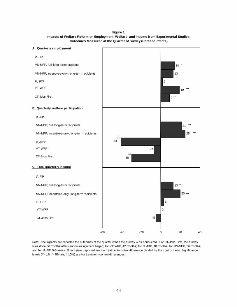
43

-5

9

0

-7

19

3

2

20

25

13

13

21

14

-30

-41

-60 -40 -20 0 20 40

Figure 1Impacts of Welfare Reform on Employment, Welfare, and Income from Experimental Studies,

Outcomes Measured at the Quarter of Survey (Percent Effects)

A. Quarterly employment

B. Quarterly welfare participation

C. Total quarterly income

Note: The impacts are reported the outcomes at the quarter w hen the survey w as conducted. For CT-Jobs First, the survey w as done 36 months after random assignment began; for VT-WRP, 42 months; for FL-FTP, 48 months; for MN-MFIP, 36 months; and for IA-FIP, 5-6 years. Effect sizes reported are the treatment-control difference divided by the control mean. Signif icance levels (*** 1%, ** 5% and * 10%) are for treatment-control differences.

IA-FIP

MN-MFIP, full, long-term recipients

MN-MFIP, incentives-only, long-term recipients

FL-FTP

VT-WRP

CT-Jobs First

IA-FIP

MN-MFIP, full, long-term recipients

MN-MFIP, incentives-only, long-term recipients

FL-FTP

VT-WRP

CT-Jobs First

IA-FIP

MN-MFIP, full, long-term recipients

MN-MFIP, incentives-only, long-term recipients

FL-FTP

VT-WRP

CT-Jobs First

***

*

**

***

***

***

***

***

**

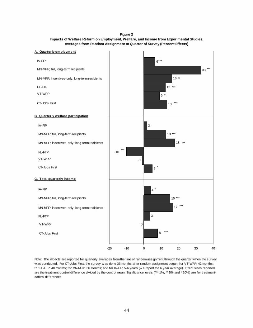
44

8

5

13

0

-1

9

3

12

17

18

16

15

13

33

4

2

6

-10

-20 -10 0 10 20 30 40

Figure 2Impacts of Welfare Reform on Employment, Welfare, and Income from Experimental Studies,

Averages from Random Assignment to Quarter of Survey (Percent Effects)

A. Quarterly employment

B. Quarterly welfare participation

C. Total quarterly income

Note: The impacts are reported for quarterly averages from the time of random assignment through the quarter w hen the survey w as conducted. For CT-Jobs First, the survey w as done 36 months after random assignment began; for VT-WRP, 42 months; for FL-FTP, 48 months; for MN-MFIP, 36 months; and for IA-FIP, 5-6 years (w e report the 6 year average). Effect sizes reported are the treatment-control difference divided by the control mean. Signif icance levels (*** 1%, ** 5% and * 10%) are for treatment-control differences.

IA-FIP

MN-MFIP, full, long-term recipients

MN-MFIP, incentives-only, long-term recipients

FL-FTP

VT-WRP

CT-Jobs First

IA-FIP

MN-MFIP, full, long-term recipients

MN-MFIP, incentives-only, long-term recipients

FL-FTP

VT-WRP

CT-Jobs First

IA-FIP

MN-MFIP, full, long-term recipients

MN-MFIP, incentives-only, long-term recipients

FL-FTP

VT-WRP

CT-Jobs First

***

*

***

**

***

***

*

*

***

***

***

***

***

***

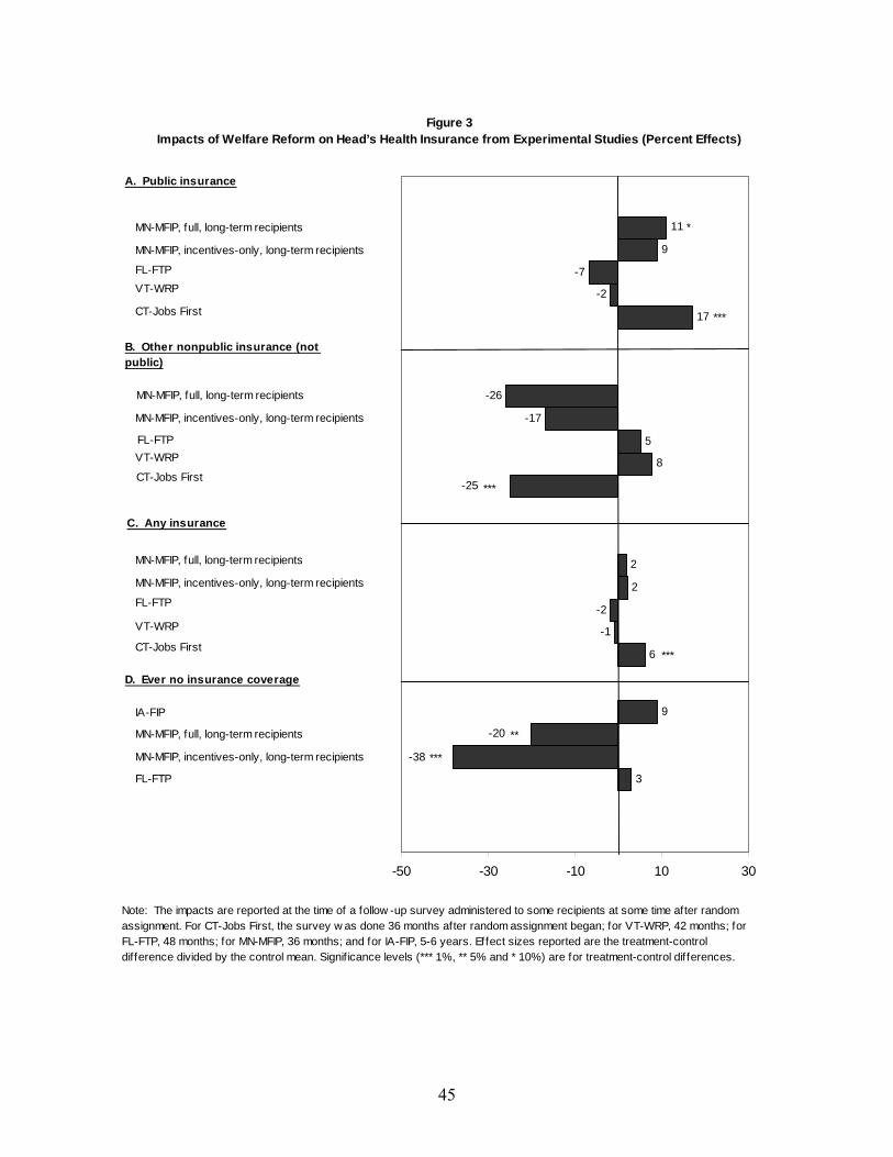
45

6

17

-1

8

-2

3

-2

5

-7

2

-17

9

2

-26

11

9

-25

-38

-20

-50 -30 -10 10 30

A. Public insurance

B. Other nonpublic insurance (not public)

C. Any insurance

D. Ever no insurance coverage

Figure 3Impacts of Welfare Reform on Head’s Health Insurance from Experimental Studies (Percent Effects)

MN-MFIP, full, long-term recipients

MN-MFIP, incentives-only, long-term recipients

FL-FTPVT-WRP

CT-Jobs First

MN-MFIP, full, long-term recipients

MN-MFIP, incentives-only, long-term recipients

FL-FTP VT-WRP

CT-Jobs First

IA-FIP

MN-MFIP, full, long-term recipients

MN-MFIP, incentives-only, long-term recipients

FL-FTP

***

***

***

***

**

*

Note: The impacts are reported at the time of a follow -up survey administered to some recipients at some time after random assignment. For CT-Jobs First, the survey w as done 36 months after random assignment began; for VT-WRP, 42 months; for FL-FTP, 48 months; for MN-MFIP, 36 months; and for IA-FIP, 5-6 years. Effect sizes reported are the treatment-control difference divided by the control mean. Signif icance levels (*** 1%, ** 5% and * 10%) are for treatment-control differences.

MN-MFIP, full, long-term recipients

MN-MFIP, incentives-only, long-term recipients

FL-FTP

VT-WRP

CT-Jobs First

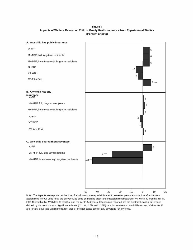
46

1

7

-1

-4

-2

-6

1

6

2

6

8

1

6

-44

-27

-50 -40 -30 -20 -10 0 10 20

Figure 4Impacts of Welfare Reform on Child or Family Health Insurance from Experimental Studies

(Percent Effects)

A. Any child has public Insurance

IA-FIP

MN-MFIP, full, long-term recipients

MN-MFIP, incentives-only, long-term recipients

FL-FTP

VT-WRP

CT-Jobs First

B. Any child has any insurance

IA-FIP

MN-MFIP, full, long-term recipients

MN-MFIP, incentives-only, long-term recipients

FL-FTP

VT-WRP

CT-Jobs First

C. Any child ever w ithout coverage

IA-FIP

MN-MFIP, full, long-term recipients

MN-MFIP, incentives-only, long-term recipients

***

***

Note: The impacts are reported at the time of a follow -up survey administered to some recipients at some time after random assignment. For CT-Jobs First, the survey w as done 36 months after random assignment began; for VT-WRP, 42 months; for FLFTP, 48 months; for MN-MFIP, 36 months; and for IA-FIP, 5-6 years. Effect sizes reported are the treatment-control difference divided by the control mean. Signif icance levels (*** 1%, ** 5% and * 10%) are for treatment-control differences. Values for IA are for any coverage w ithin the family, those for other states are for any coverage for any child.

**

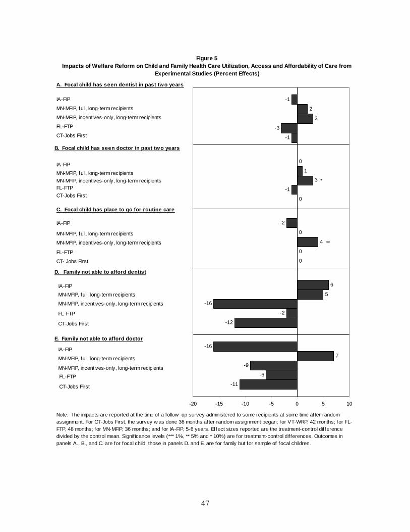
47

-11

-12

0

0

-1

-6

-2

0

-1

-3

-9

-16

4

3

3

7

5

0

1

2

-16

6

-2

0

-1

-20 -15 -10 -5 0 5 10

Figure 5Impacts of Welfare Reform on Child and Family Health Care Utilization, Access and Affordability of Care from

Experimental Studies (Percent Effects)

A. Focal child has seen dentist in past two years

IA-FIP

MN-MFIP, full, long-term recipients

MN-MFIP, incentives-only, long-term recipients

FL-FTP

CT-Jobs First

B. Focal child has seen doctor in past two years

IA-FIPMN-MFIP, full, long-term recipientsMN-MFIP, incentives-only, long-term recipientsFL-FTPCT-Jobs First

C. Focal child has place to go for routine care

MN-MFIP, full, long-term recipients

MN-MFIP, incentives-only, long-term recipients

FL-FTP

CT- Jobs First

D. Family not able to afford dentist

IA-FIP

IA-FIPMN-MFIP, full, long-term recipients

MN-MFIP, incentives-only, long-term recipients

FL-FTP

CT-Jobs First

E. Family not able to afford doctor

IA-FIP

MN-MFIP, full, long-term recipients

MN-MFIP, incentives-only, long-term recipientsFL-FTP

CT-Jobs First

**

*

Note: The impacts are reported at the time of a follow -up survey administered to some recipients at some time after random assignment. For CT-Jobs First, the survey w as done 36 months after random assignment began; for VT-WRP, 42 months; for FL-FTP, 48 months; for MN-MFIP, 36 months; and for IA-FIP, 5-6 years. Effect sizes reported are the treatment-control difference divided by the control mean. Signif icance levels (*** 1%, ** 5% and * 10%) are for treatment-control differences. Outcomes in panels A., B., and C. are for focal child, those in panels D. and E. are for family but for sample of focal children.

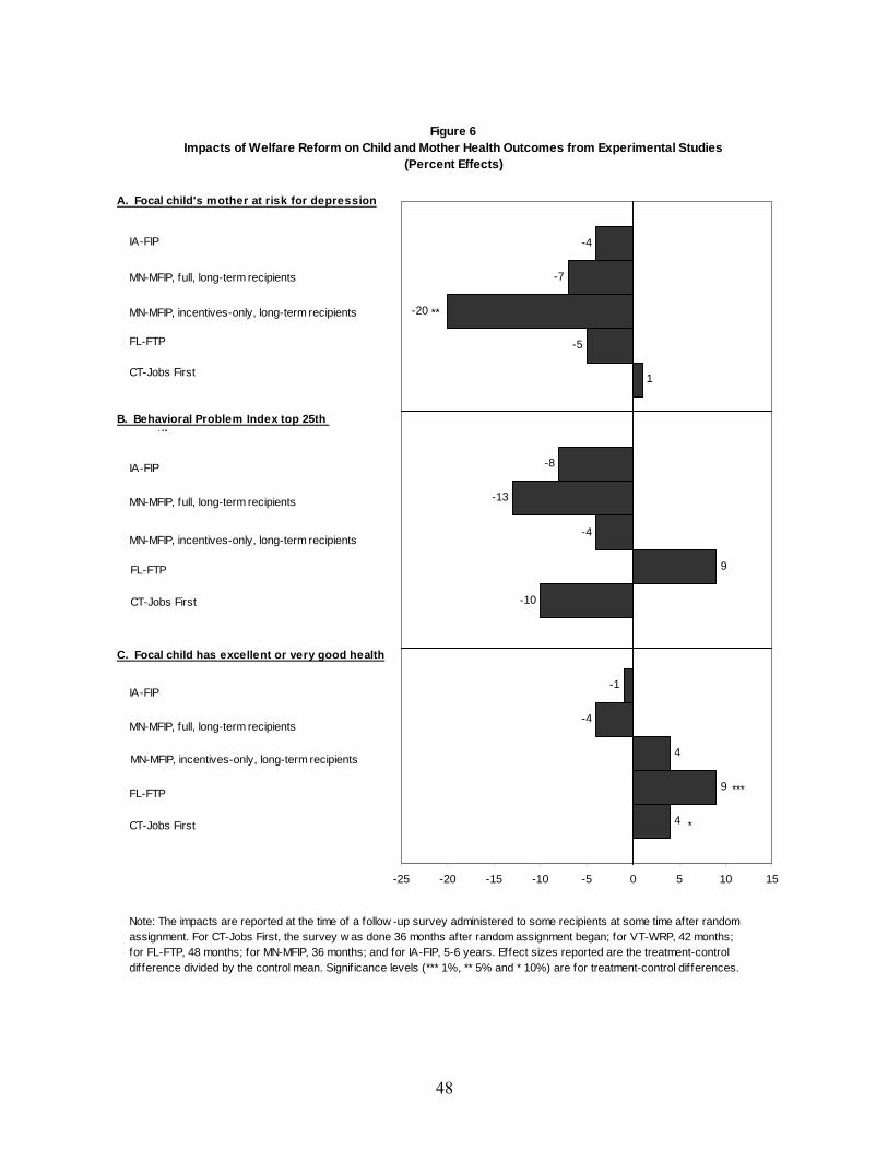
48

4

-10

1

9

9

-5

4

-4

-4

-13

-7

-1

-8

-4

-20

-25 -20 -15 -10 -5 0 5 10 15

Figure 6Impacts of Welfare Reform on Child and Mother Health Outcomes from Experimental Studies

(Percent Effects)

A. Focal child's mother at risk for depression

B. Behavioral Problem Index top 25th til

C. Focal child has excellent or very good health

*

***

**

Note: The impacts are reported at the time of a follow -up survey administered to some recipients at some time after random assignment. For CT-Jobs First, the survey w as done 36 months after random assignment began; for VT-WRP, 42 months; for FL-FTP, 48 months; for MN-MFIP, 36 months; and for IA-FIP, 5-6 years. Effect sizes reported are the treatment-control dif ference divided by the control mean. Signif icance levels (*** 1%, ** 5% and * 10%) are for treatment-control differences.

IA-FIP

MN-MFIP, full, long-term recipients

MN-MFIP, incentives-only, long-term recipients

FL-FTP

CT-Jobs First

IA-FIP

MN-MFIP, full, long-term recipients

MN-MFIP, incentives-only, long-term recipients

FL-FTP

CT-Jobs First

IA-FIP

MN-MFIP, full, long-term recipients

MN-MFIP, incentives-only, long-term recipients

FL-FTP

CT-Jobs First

Table 1: Policies in Welfare Reform Experiments and Preexisting AFDC Program Connecticut

Jobs First (JF) Florida Family

Transition Program (FTP)

Minnesota Family Investment Program

(MFIP)

Iowa Family Investment Program (FIP)

Vermont Welfare Restructuring Project

(WRP)

General Two tiered system based on job readiness

Two tiered system for long term/short term recipients; Two treatments incentives only and full

Control group subject to TANF rules in 97

Two treatments: incentives only and full(we only consider full treatment)

Time Limit 21 months with 6 months extensions

24 months (of every 60)for job ready; 36 (of every 72) months for others

None

None None

Work Requirements Mandatory work first, exempt if child < 1 year

Mandatory job search & employment for job ready; education and training for others; exempt if child < 6 months

Mandatory employment and training for long term; exempt if child < 1 year

Employment and training; exempt if child < 6 months (eliminated in 97)

Half time work required after 30 months on aid

Earnings Disregards All earnings disregarded until poverty line

$200 + 50% of remaining earnings

38% of earnings disregarded up to 140% of poverty; maximum grant increased by 20% if working

40% of earnings disregarded (all earnings disregarded for 1st 4 months of work if “new worker” through 97)

$150 + 25% of remaining earnings

Financial Sanctions Cut in grant for 1st and 2nd offense; 3 mo. suspension for 3rd

Adult portion of grant eliminated until compliant (until 6/97)

10% reduction in grant

3 months reduced benefits, 6 months no benefits

None

Selected other policies Two years transitional Medicaid

One year transitional Medicaid

One year transitional Medicaid

One year transitional Medicaid

3 years transitional Medicaid

Benefit level, family of 3 at start of experiment

$636 $303 $532

$426 $640

Sources: Dan Bloom et al., (2000); Bloom et al., (2002); Thomas Fraker et al., (2002); Gennetian et al., (2005) ; and Susan Scrivener et al., (2002).

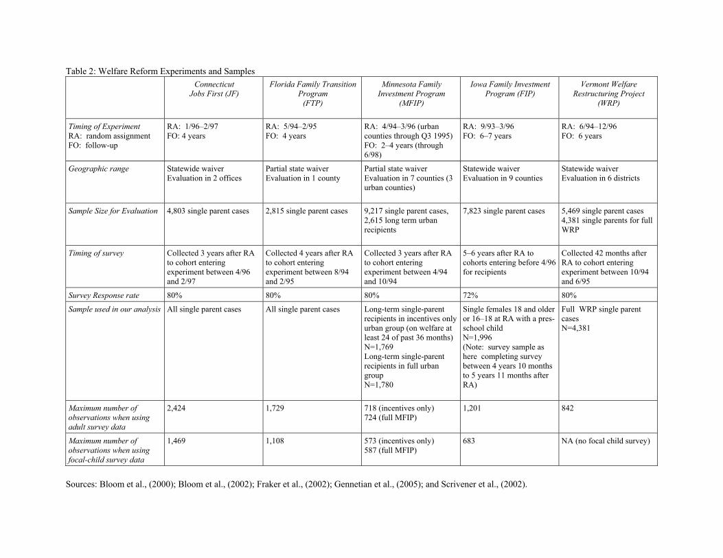
Table 2: Welfare Reform Experiments and Samples Connecticut

Jobs First (JF) Florida Family Transition

Program (FTP)

Minnesota Family Investment Program

(MFIP)

Iowa Family Investment Program (FIP)

Vermont Welfare Restructuring Project

(WRP)

Timing of Experiment RA: random assignment FO: follow-up

RA: 1/96–2/97 FO: 4 years

RA: 5/94–2/95 FO: 4 years

RA: 4/94–3/96 (urban counties through Q3 1995) FO: 2–4 years (through 6/98)

RA: 9/93–3/96 FO: 6–7 years

RA: 6/94–12/96 FO: 6 years

Geographic range Statewide waiver Evaluation in 2 offices

Partial state waiver Evaluation in 1 county

Partial state waiver Evaluation in 7 counties (3 urban counties)

Statewide waiver Evaluation in 9 counties

Statewide waiver Evaluation in 6 districts

Sample Size for Evaluation 4,803 single parent cases

2,815 single parent cases

9,217 single parent cases, 2,615 long term urban recipients

7,823 single parent cases 5,469 single parent cases 4,381 single parents for full WRP

Timing of survey Collected 3 years after RA to cohort entering experiment between 4/96 and 2/97

Collected 4 years after RA to cohort entering experiment between 8/94 and 2/95

Collected 3 years after RA to cohort entering experiment between 4/94 and 10/94

5–6 years after RA to cohorts entering before 4/96 for recipients

Collected 42 months after RA to cohort entering experiment between 10/94 and 6/95

Survey Response rate 80% 80% 80% 72% 80%

Sample used in our analysis All single parent cases All single parent cases Long-term single-parent recipients in incentives only urban group (on welfare at least 24 of past 36 months) N=1,769 Long-term single-parent recipients in full urban group N=1,780

Single females 18 and older or 16–18 at RA with a pres-school child N=1,996 (Note: survey sample as here completing survey between 4 years 10 months to 5 years 11 months after RA)

Full WRP single parent cases N=4,381

Maximum number of observations when using adult survey data

2,424 1,729 718 (incentives only) 724 (full MFIP)

1,201 842

Maximum number of observations when using focal-child survey data

1,469 1,108 573 (incentives only) 587 (full MFIP)

683 NA (no focal child survey)

Sources: Bloom et al., (2000); Bloom et al., (2002); Fraker et al., (2002); Gennetian et al., (2005); and Scrivener et al., (2002).

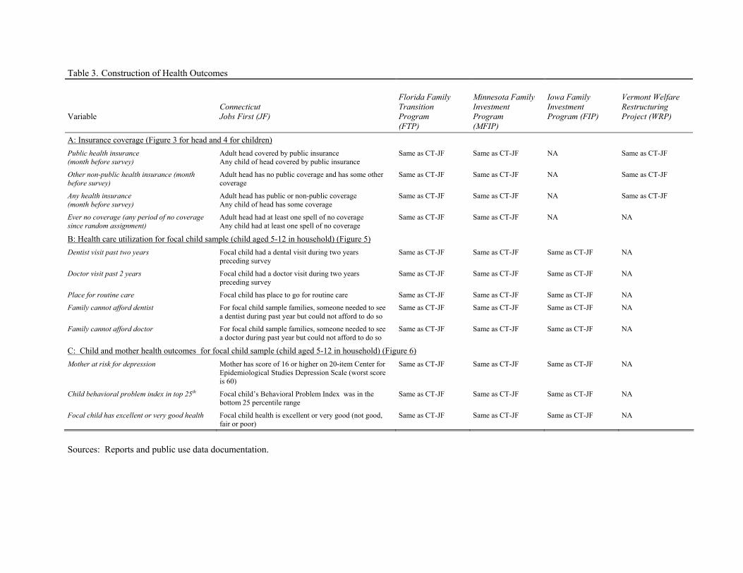
Table 3. Construction of Health Outcomes Variable

Connecticut Jobs First (JF)

Florida Family Transition Program (FTP)

Minnesota Family Investment Program (MFIP)

Iowa Family Investment Program (FIP)

Vermont Welfare Restructuring Project (WRP)

A: Insurance coverage (Figure 3 for head and 4 for children) Public health insurance (month before survey)

Adult head covered by public insurance Any child of head covered by public insurance

Same as CT-JF Same as CT-JF NA Same as CT-JF

Other non-public health insurance (month before survey)

Adult head has no public coverage and has some other coverage

Same as CT-JF Same as CT-JF

NA Same as CT-JF

Any health insurance (month before survey)

Adult head has public or non-public coverage Any child of head has some coverage

Same as CT-JF Same as CT-JF

NA Same as CT-JF

Ever no coverage (any period of no coverage since random assignment)

Adult head had at least one spell of no coverage Any child had at least one spell of no coverage

Same as CT-JF Same as CT-JF NA NA

B: Health care utilization for focal child sample (child aged 5-12 in household) (Figure 5) Dentist visit past two years Focal child had a dental visit during two years

preceding survey Same as CT-JF Same as CT-JF

Same as CT-JF NA

Doctor visit past 2 years Focal child had a doctor visit during two years preceding survey

Same as CT-JF Same as CT-JF Same as CT-JF NA

Place for routine care Focal child has place to go for routine care Same as CT-JF Same as CT-JF Same as CT-JF NA

Family cannot afford dentist For focal child sample families, someone needed to see a dentist during past year but could not afford to do so

Same as CT-JF Same as CT-JF

Same as CT-JF NA

Family cannot afford doctor For focal child sample families, someone needed to see a doctor during past year but could not afford to do so

Same as CT-JF Same as CT-JF Same as CT-JF NA

C: Child and mother health outcomes for focal child sample (child aged 5-12 in household) (Figure 6) Mother at risk for depression Mother has score of 16 or higher on 20-item Center for

Epidemiological Studies Depression Scale (worst score is 60)

Same as CT-JF Same as CT-JF Same as CT-JF NA

Child behavioral problem index in top 25th Focal child’s Behavioral Problem Index was in the bottom 25 percentile range

Same as CT-JF Same as CT-JF Same as CT-JF NA

Focal child has excellent or very good health Focal child health is excellent or very good (not good, fair or poor)

Same as CT-JF Same as CT-JF Same as CT-JF NA

Sources: Reports and public use data documentation.

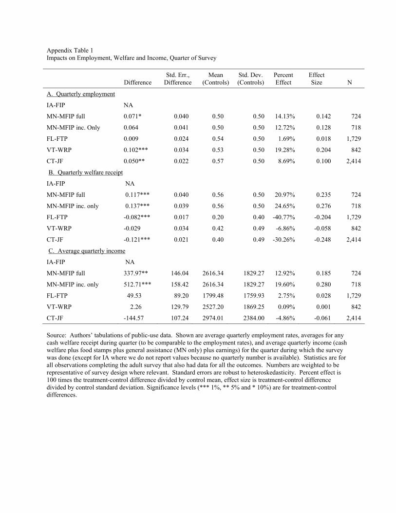
Appendix Table 1 Impacts on Employment, Welfare and Income, Quarter of Survey

Difference Std. Err.,

Difference Mean

(Controls) Std. Dev. (Controls)

Percent Effect

Effect Size

N

A. Quarterly employment

IA-FIP NA

MN-MFIP full 0.071* 0.040 0.50 0.50 14.13% 0.142 724

MN-MFIP inc. Only 0.064 0.041 0.50 0.50 12.72% 0.128 718

FL-FTP 0.009 0.024 0.54 0.50 1.69% 0.018 1,729

VT-WRP 0.102*** 0.034 0.53 0.50 19.28% 0.204 842

CT-JF 0.050** 0.022 0.57 0.50 8.69% 0.100 2,414

B. Quarterly welfare receipt

IA-FIP NA

MN-MFIP full 0.117*** 0.040 0.56 0.50 20.97% 0.235 724

MN-MFIP inc. only 0.137*** 0.039 0.56 0.50 24.65% 0.276 718

FL-FTP -0.082*** 0.017 0.20 0.40 -40.77% -0.204 1,729

VT-WRP -0.029 0.034 0.42 0.49 -6.86% -0.058 842

CT-JF -0.121*** 0.021 0.40 0.49 -30.26% -0.248 2,414

C. Average quarterly income

IA-FIP NA

MN-MFIP full 337.97** 146.04 2616.34 1829.27 12.92% 0.185 724

MN-MFIP inc. only 512.71*** 158.42 2616.34 1829.27 19.60% 0.280 718

FL-FTP 49.53 89.20 1799.48 1759.93 2.75% 0.028 1,729

VT-WRP 2.26 129.79 2527.20 1869.25 0.09% 0.001 842

CT-JF -144.57 107.24 2974.01 2384.00 -4.86% -0.061 2,414 Source: Authors’ tabulations of public-use data. Shown are average quarterly employment rates, averages for any cash welfare receipt during quarter (to be comparable to the employment rates), and average quarterly income (cash welfare plus food stamps plus general assistance (MN only) plus earnings) for the quarter during which the survey was done (except for IA where we do not report values because no quarterly number is available). Statistics are for all observations completing the adult survey that also had data for all the outcomes. Numbers are weighted to be representative of survey design where relevant. Standard errors are robust to heteroskedasticity. Percent effect is 100 times the treatment-control difference divided by control mean, effect size is treatment-control difference divided by control standard deviation. Significance levels (*** 1%, ** 5% and * 10%) are for treatment-control differences.

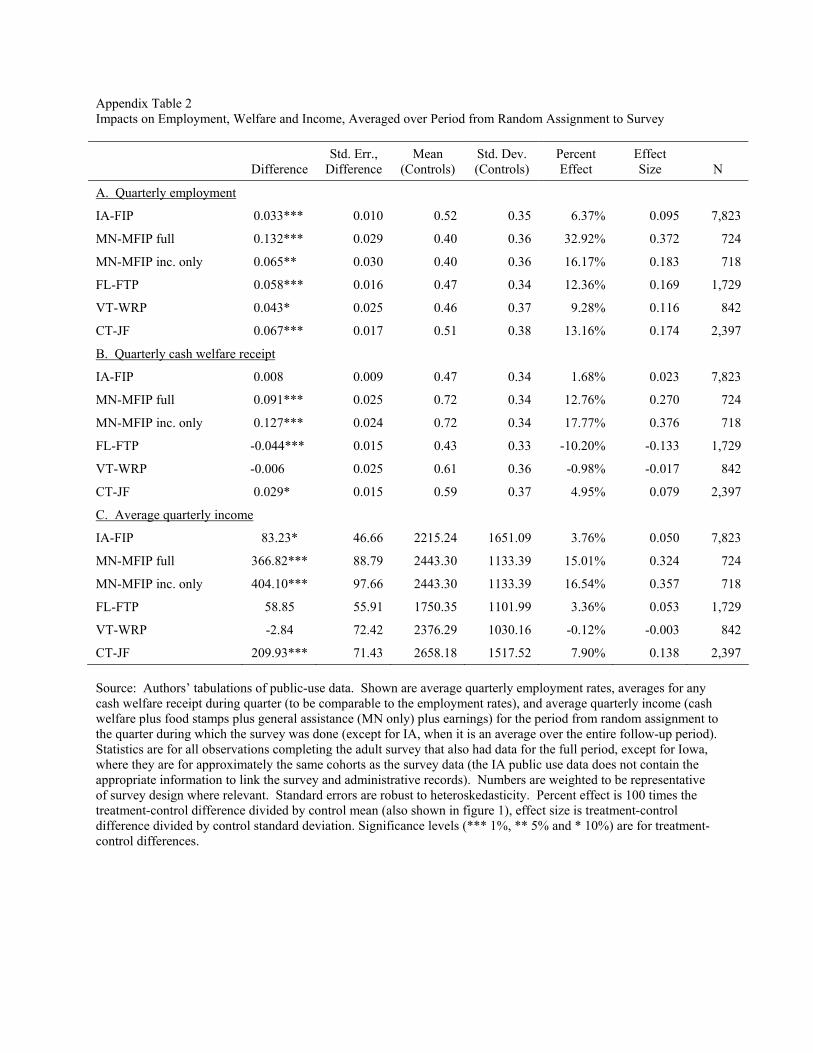
Appendix Table 2 Impacts on Employment, Welfare and Income, Averaged over Period from Random Assignment to Survey

Difference Std. Err.,

Difference Mean

(Controls) Std. Dev. (Controls)

Percent Effect

Effect Size

N

A. Quarterly employment

IA-FIP 0.033*** 0.010 0.52 0.35 6.37% 0.095 7,823

MN-MFIP full 0.132*** 0.029 0.40 0.36 32.92% 0.372 724

MN-MFIP inc. only 0.065** 0.030 0.40 0.36 16.17% 0.183 718

FL-FTP 0.058*** 0.016 0.47 0.34 12.36% 0.169 1,729

VT-WRP 0.043* 0.025 0.46 0.37 9.28% 0.116 842

CT-JF 0.067*** 0.017 0.51 0.38 13.16% 0.174 2,397

B. Quarterly cash welfare receipt

IA-FIP 0.008 0.009 0.47 0.34 1.68% 0.023 7,823

MN-MFIP full 0.091*** 0.025 0.72 0.34 12.76% 0.270 724

MN-MFIP inc. only 0.127*** 0.024 0.72 0.34 17.77% 0.376 718

FL-FTP -0.044*** 0.015 0.43 0.33 -10.20% -0.133 1,729

VT-WRP -0.006 0.025 0.61 0.36 -0.98% -0.017 842

CT-JF 0.029* 0.015 0.59 0.37 4.95% 0.079 2,397

C. Average quarterly income

IA-FIP 83.23* 46.66 2215.24 1651.09 3.76% 0.050 7,823

MN-MFIP full 366.82*** 88.79 2443.30 1133.39 15.01% 0.324 724

MN-MFIP inc. only 404.10*** 97.66 2443.30 1133.39 16.54% 0.357 718

FL-FTP 58.85 55.91 1750.35 1101.99 3.36% 0.053 1,729

VT-WRP -2.84 72.42 2376.29 1030.16 -0.12% -0.003 842

CT-JF 209.93*** 71.43 2658.18 1517.52 7.90% 0.138 2,397 Source: Authors’ tabulations of public-use data. Shown are average quarterly employment rates, averages for any cash welfare receipt during quarter (to be comparable to the employment rates), and average quarterly income (cash welfare plus food stamps plus general assistance (MN only) plus earnings) for the period from random assignment to the quarter during which the survey was done (except for IA, when it is an average over the entire follow-up period). Statistics are for all observations completing the adult survey that also had data for the full period, except for Iowa, where they are for approximately the same cohorts as the survey data (the IA public use data does not contain the appropriate information to link the survey and administrative records). Numbers are weighted to be representative of survey design where relevant. Standard errors are robust to heteroskedasticity. Percent effect is 100 times the treatment-control difference divided by control mean (also shown in figure 1), effect size is treatment-control difference divided by control standard deviation. Significance levels (*** 1%, ** 5% and * 10%) are for treatment-control differences.

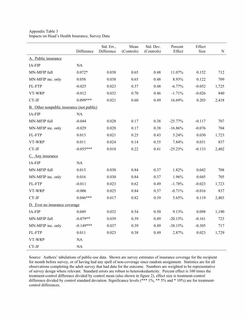
Appendix Table 3 Impacts on Head’s Health Insurance, Survey Data

Difference Std. Err.,

Difference Mean

(Controls) Std. Dev.

(Controls) Percent

Effect Effect

Size

N

A. Public insurance

IA-FIP NA

MN-MFIP full 0.072* 0.038 0.65 0.48 11.07% 0.152 712

MN-MFIP inc. only 0.058 0.038 0.65 0.48 8.93% 0.122 709

FL-FTP -0.025 0.023 0.37 0.48 -6.77% -0.052 1,725

VT-WRP -0.012 0.032 0.70 0.46 -1.71% -0.026 840

CT-JF 0.099*** 0.021 0.60 0.49 16.69% 0.203 2,418

B. Other nonpublic insurance (not public)

IA-FIP NA

MN-MFIP full -0.044 0.028 0.17 0.38 -25.77% -0.117 707

MN-MFIP inc. only -0.029 0.028 0.17 0.38 -16.86% -0.076 704

FL-FTP 0.013 0.021 0.25 0.43 5.24% 0.030 1,723

VT-WRP 0.011 0.024 0.14 0.35 7.84% 0.031 837

CT-JF -0.055*** 0.018 0.22 0.41 -25.23% -0.133 2,402

C. Any insurance

IA-FIP NA

MN-MFIP full 0.015 0.030 0.84 0.37 1.82% 0.042 708

MN-MFIP inc. only 0.016 0.030 0.84 0.37 1.96% 0.045 705

FL-FTP -0.011 0.023 0.62 0.49 -1.78% -0.023 1,723

VT-WRP -0.006 0.025 0.84 0.37 -0.71% -0.016 837

CT-JF 0.046*** 0.017 0.82 0.39 5.65% 0.119 2,403

D. Ever no insurance coverage

IA-FIP 0.049 0.032 0.54 0.50 9.13% 0.098 1,190

MN-MFIP full -0.079** 0.039 0.39 0.49 -20.15% -0.161 723

MN-MFIP inc. only -0.149*** 0.037 0.39 0.49 -38.15% -0.305 717

FL-FTP 0.011 0.023 0.38 0.49 2.87% 0.023 1,729

VT-WRP NA

CT-JF NA Source: Authors’ tabulations of public-use data. Shown are survey estimates of insurance coverage for the recipient for month before survey, or of having had any spell of non-coverage since random assignment. Statistics are for all observations completing the adult survey that had data for the outcome. Numbers are weighted to be representative of survey design where relevant. Standard errors are robust to heteroskedasticity. Percent effect is 100 times the treatment-control difference divided by control mean (also shown in figure 2), effect size is treatment-control difference divided by control standard deviation. Significance levels (*** 1%, ** 5% and * 10%) are for treatment-control differences.

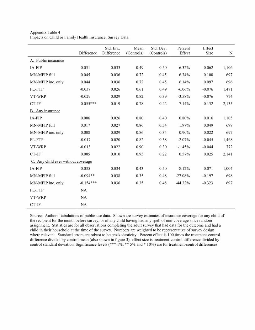
Appendix Table 4 Impacts on Child or Family Health Insurance, Survey Data

Difference Std. Err.,

Difference Mean

(Controls) Std. Dev.

(Controls) Percent

Effect Effect

Size

N

A. Public insurance

IA-FIP 0.031 0.033 0.49 0.50 6.32% 0.062 1,106

MN-MFIP full 0.045 0.036 0.72 0.45 6.34% 0.100 697

MN-MFIP inc. only 0.044 0.036 0.72 0.45 6.14% 0.097 696

FL-FTP -0.037 0.026 0.61 0.49 -6.06% -0.076 1,471

VT-WRP -0.029 0.029 0.82 0.39 -3.58% -0.076 774

CT-JF 0.055*** 0.019 0.78 0.42 7.14% 0.132 2,135

B. Any insurance

IA-FIP 0.006 0.026 0.80 0.40 0.80% 0.016 1,105

MN-MFIP full 0.017 0.027 0.86 0.34 1.97% 0.049 698

MN-MFIP inc. only 0.008 0.029 0.86 0.34 0.90% 0.022 697

FL-FTP -0.017 0.020 0.82 0.38 -2.07% -0.045 1,468

VT-WRP -0.013 0.022 0.90 0.30 -1.45% -0.044 772

CT-JF 0.005 0.010 0.95 0.22 0.57% 0.025 2,141

C. Any child ever without coverage

IA-FIP 0.035 0.034 0.43 0.50 8.12% 0.071 1,004

MN-MFIP full -0.094** 0.038 0.35 0.48 -27.08% -0.197 698

MN-MFIP inc. only -0.154*** 0.036 0.35 0.48 -44.32% -0.323 697

FL-FTP NA

VT-WRP NA

CT-JF NA Source: Authors’ tabulations of public-use data. Shown are survey estimates of insurance coverage for any child of the recipient for the month before survey, or of any child having had any spell of non-coverage since random assignment. Statistics are for all observations completing the adult survey that had data for the outcome and had a child in their household at the time of the survey. Numbers are weighted to be representative of survey design where relevant. Standard errors are robust to heteroskedasticity. Percent effect is 100 times the treatment-control difference divided by control mean (also shown in figure 3), effect size is treatment-control difference divided by control standard deviation. Significance levels (*** 1%, ** 5% and * 10%) are for treatment-control differences.

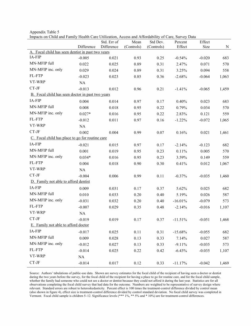
Appendix Table 5 Impacts on Child and Family Health Care Utilization, Access and Affordability of Care, Survey Data

Difference Std. Err of Difference

Mean (Controls)

Std Dev. (Controls)

Percent Effect

Effect Size

N

A. Focal child has seen dentist in past two years IA-FIP -0.005 0.021 0.93 0.25 -0.54% -0.020 683 MN-MFIP full 0.022 0.025 0.89 0.31 2.47% 0.071 570 MN-MFIP inc. only 0.029 0.024 0.89 0.31 3.25% 0.094 558 FL-FTP -0.023 0.023 0.85 0.36 -2.68% -0.064 1,063 VT-WRP NA CT-JF -0.013 0.012 0.96 0.21 -1.41% -0.065 1,459 B. Focal child has seen doctor in past two years

IA-FIP 0.004 0.014 0.97 0.17 0.40% 0.023 683 MN-MFIP full 0.008 0.018 0.95 0.22 0.79% 0.034 570 MN-MFIP inc. only 0.027* 0.016 0.95 0.22 2.83% 0.121 559 FL-FTP -0.012 0.011 0.97 0.16 -1.22% -0.072 1,065 VT-WRP NA CT-JF 0.002 0.004 0.99 0.07 0.16% 0.021 1,461 C. Focal child has place to go for routine care

IA-FIP -0.021 0.015 0.97 0.17 -2.14% -0.123 682 MN-MFIP full 0.001 0.019 0.95 0.23 0.11% 0.005 570 MN-MFIP inc. only 0.034* 0.016 0.95 0.23 3.59% 0.149 559 FL-FTP 0.004 0.018 0.90 0.30 0.41% 0.012 1,067 VT-WRP NA CT-JF -0.004 0.006 0.99 0.11 -0.37% -0.035 1,460 D. Family not able to afford dentist

IA-FIP 0.009 0.031 0.17 0.37 5.62% 0.025 682 MN-MFIP full 0.010 0.033 0.20 0.40 5.19% 0.026 587 MN-MFIP inc. only -0.031 0.032 0.20 0.40 -16.01% -0.079 573 FL-FTP -0.007 0.029 0.35 0.48 -2.14% -0.016 1,107 VT-WRP NA CT-JF -0.019 0.019 0.17 0.37 -11.51% -0.051 1,468 E. Family not able to afford doctor

IA-FIP -0.017 0.025 0.11 0.31 -15.68% -0.055 682 MN-MFIP full 0.009 0.028 0.13 0.33 7.14% 0.027 587 MN-MFIP inc. only -0.012 0.027 0.13 0.33 -9.11% -0.035 573 FL-FTP -0.014 0.025 0.22 0.42 -6.43% -0.035 1,107 VT-WRP NA CT-JF -0.014 0.017 0.12 0.33 -11.17% -0.042 1,469 Source: Authors’ tabulations of public-use data. Shown are survey estimates for the focal child of the recipient of having seen a doctor or dentist during the two years before the survey, for the focal child of the recipient for having a place to go for routine care, and for the focal child sample, whether the family had someone who could not see a doctor or dentist because they could not afford it during the last year. Statistics are for all observations completing the focal child survey that had data for the outcome. Numbers are weighted to be representative of survey design where relevant. Standard errors are robust to heteroskedasticity. Percent effect is 100 times the treatment-control difference divided by control mean (also shown in figure 4), effect size is treatment-control difference divided by control standard deviation. No focal child survey was completed in Vermont. Focal child sample is children 5–12. Significance levels (*** 1%, ** 5% and * 10%) are for treatment-control differences.

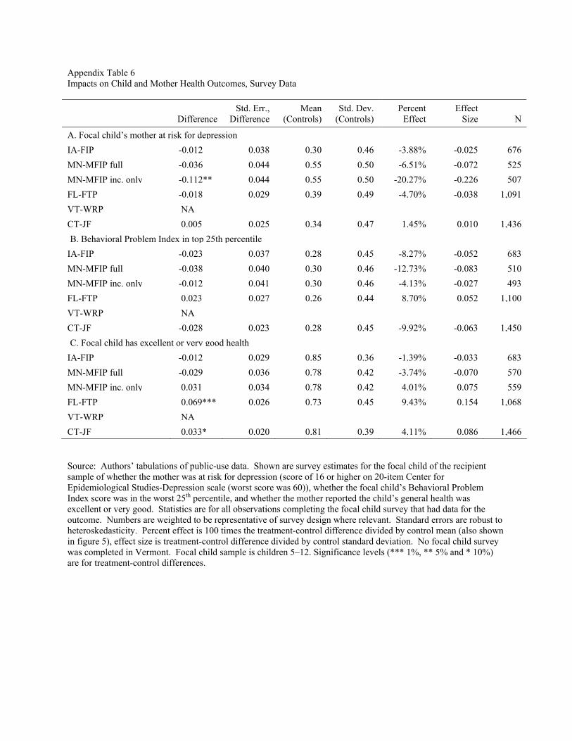
Appendix Table 6 Impacts on Child and Mother Health Outcomes, Survey Data

Difference Std. Err.,

Difference Mean

(Controls) Std. Dev.

(Controls) Percent

Effect Effect

Size

N

A. Focal child’s mother at risk for depression IA-FIP -0.012 0.038 0.30 0.46 -3.88% -0.025 676MN-MFIP full -0.036 0.044 0.55 0.50 -6.51% -0.072 525MN-MFIP inc. only -0.112** 0.044 0.55 0.50 -20.27% -0.226 507FL-FTP -0.018 0.029 0.39 0.49 -4.70% -0.038 1,091VT-WRP NA CT-JF 0.005 0.025 0.34 0.47 1.45% 0.010 1,436B. Behavioral Problem Index in top 25th percentile

IA-FIP -0.023 0.037 0.28 0.45 -8.27% -0.052 683MN-MFIP full -0.038 0.040 0.30 0.46 -12.73% -0.083 510MN-MFIP inc. only -0.012 0.041 0.30 0.46 -4.13% -0.027 493FL-FTP 0.023 0.027 0.26 0.44 8.70% 0.052 1,100VT-WRP NA CT-JF -0.028 0.023 0.28 0.45 -9.92% -0.063 1,450C. Focal child has excellent or very good health

IA-FIP -0.012 0.029 0.85 0.36 -1.39% -0.033 683MN-MFIP full -0.029 0.036 0.78 0.42 -3.74% -0.070 570MN-MFIP inc. only 0.031 0.034 0.78 0.42 4.01% 0.075 559FL-FTP 0.069*** 0.026 0.73 0.45 9.43% 0.154 1,068VT-WRP NA CT-JF 0.033* 0.020 0.81 0.39 4.11% 0.086 1,466 Source: Authors’ tabulations of public-use data. Shown are survey estimates for the focal child of the recipient sample of whether the mother was at risk for depression (score of 16 or higher on 20-item Center for Epidemiological Studies-Depression scale (worst score was 60)), whether the focal child’s Behavioral Problem Index score was in the worst 25th percentile, and whether the mother reported the child’s general health was excellent or very good. Statistics are for all observations completing the focal child survey that had data for the outcome. Numbers are weighted to be representative of survey design where relevant. Standard errors are robust to heteroskedasticity. Percent effect is 100 times the treatment-control difference divided by control mean (also shown in figure 5), effect size is treatment-control difference divided by control standard deviation. No focal child survey was completed in Vermont. Focal child sample is children 5–12. Significance levels (*** 1%, ** 5% and * 10%) are for treatment-control differences.

Appendix Table 7 Summary Measure Impacts on Adult, Child, and Family Measures, Survey Data

Difference Std. Err of Difference

FWE Adjusted p-value

N

A. Summary measure, employment, off welfare, and income, ave. since RA IA-FIP 0.041 0.020 0.181 7,823MN-MFIP full 0.113 0.051 0.115 724MN-MFIP 0.021 0.054 0.698 718FL-FTP 0.110*** 0.030 0.000 1,729VT-WRP 0.046 0.048 0.671 842CT-JF 0.078* 0.034 0.099 2,397B. Summary measure, head’s HI coverage IA-FIP -0.049 0.032 0.409 1,190MN-MFIP full 0.070 0.059 0.551 707MN-MFIP 0.118 0.059 0.125 704FL-FTP -0.021 0.051 0.900 1,723VT-WRP -0.007 0.038 0.849 837CT-JF 0.060* 0.025 0.099 2,402C. Summary measure, child/family HI coverageIA-FIP 0.001 0.050 0.993 1,105MN-MFIP full 0.114 0.062 0.235 697MN-MFIP 0.144 0.064 0.107 696FL-FTP -0.066 0.053 0.489 1,468VT-WRP -0.052 0.060 0.671 771CT-JF 0.067 0.032 0.103 2,134IA-FIP -0.013 0.045 0.993 681D. Summary measure, child/family utilization, access, and affordabilityMN-MFIP full 0.015 0.058 0.857 570MN-MFIP 0.117 0.055 0.123 558FL-FTP -0.018 0.045 0.900 1,060VT-WRP NA CT-JF 0.006 0.024 0.801 1,453E. Summary measure, child/mother health IA-FIP 0.015 0.054 0.993 676MN-MFIP full 0.030 0.062 0.857 509MN-MFIP 0.120 0.062 0.125 492FL-FTP 0.065 0.044 0.435 1,048VT-WRP NA CT-JF 0.051 0.036 0.263 1,421 Source: Authors’ tabulations of public-use data. Shown are survey estimates for summary measures for each state for each of the variables presented in figures 2–6. Each summary measure is the average of the outcomes on each figure (normalized by each outcome’s control standard deviation), after converting each outcome to be positive when good (welfare participation is considered bad, but any kind of HI good). For the figure 2 summary measure,

the sample is adults completing the survey with non-missing administrative data (for IA only, it is instead the same cohort as the survey). For the figure 3 summary measure, the sample is adults completing the survey with non-missing HI data. For the figure 4 summary measure, the sample is adults with a child in the HH at the time of the survey completing the survey with non-missing child/family HI coverage data. For the figures 5 and 6 summary measures, the sample is survey recipients with a focal child completing the survey, with non-missing data on health care utilization, access, and affordability or health outcomes, respectively. Numbers are weighted to be representative of survey design where relevant. Standard errors are robust to heteroskedasticity. Difference is treatment control difference in each summary measure. FWE adjusted p-value is p-value for comparison in row, adjusted for joint testing across all summary measures in the state. No focal child survey was completed in Vermont. Focal child sample is children 5–12. Significance levels (*** 1%, ** 5% and * 10%) are for treatment-control differences, adjusted for family-wise errors.