Weighted Marshall-Olkin Bivariate

Exponential Distribution

Ahad Jamalizadeh§ & Debasis Kundu†

Abstract

Recently Gupta and Kundu [9] introduced a new class of weighted exponential dis-tributions, and it can be used quite effectively to model lifetime data. In this paper,we introduce a new class of weighted Marshall-Olkin bivariate exponential distribu-tions. This new singular distribution has univariate weighted exponential marginals.We study different properties of the proposed model. There are four parameters in thismodel and the maximum likelihood estimators (MLEs) of the unknown parameterscannot be obtained in explicit forms. We need to solve a four dimensional optimiza-tion problem to compute the MLEs. One data set has been analyzed for illustrativepurposes and finally we propose some generalization of the proposed model.

Keywords: Joint probability density function; Conditional probability density function;

Singular distribution; Maximum likelihood estimators; Fisher information matrix; Asymp-

totic distribution.

§Department of Statistics, Faculty of Mathematics & Computer, Shahid Bahonar University

of Kerman, Kerman,Iran,76169-14111.

†Department of Mathematics and Statistics, Indian Institute of Technology Kanpur, Pin

208016, India, e-mail: kundu@iitk.ac.in. Visiting Professor at the King Saud University,

Saudi Arabia. Corresponding author. Part of this work is supported by a grant from the

Department of Science and Technology, Government of India.

1

2

1 Introduction

Recently Gupta and Kundu [9] introduced a shape parameter to an exponential distribution

using the idea of Azzalini [5] and study its different properties. This new class of distributions

turn out to be a weighted exponential distributions, and due to this reason it is named as

the weighted exponential (WE) distribution. Several interesting properties of this new WE

distribution have been established by Gupta and Kundu [9]. It is observed that the two-

parameter WE distribution distribution behaves very similarly, with the other well known

two-parameter distributions, like Weibull, gamma or generalized exponential distributions

and it has several desirable properties also. The WE distribution can be obtained as a

hidden truncation model. Moreover, it has been observed that in certain cases the two-

parameter WE distribution may provide a better fit than the two-parameter Weibull, gamma

or generalized exponential distributions. Since, its distribution function is in compact form,

it can be used very effectively to analyze censored data also. A brief review of the two-

parameter WE distribution is presented in section 2, for ready reference.

Recently, Al-Mutairi et al. [2] introduced an absolute continuous bivariate distribution

with weighted exponential marginals. The main aim of this paper is to introduce a weighted

Marshall-Olkin bivariate exponential (WMOBE) distribution, using the similar idea as of

Azzalini [5], and it is quite different than the method proposed by Al-Mutairi et al. [2].

This new singular WMOBE distribution has four parameters. It can also be obtained as a

hidden truncation model as of Arnold and Beaver [3]. Therefore, the interpretation of any

multivariate hidden truncation model as it was provided by Arnold and Beaver [4] is valid

for this proposed model also. This is one of the basic motivations of the proposed model.

Moreover, it may be mentioned that the most popular singular bivariate distribution is

the three-parameter Marshall-Olkin bivariate exponential (MOBE) distribution or the four-

3

parameter Marshall-Olkin bivariate Weibull (MOBW) distribution, see for example Kotz et

al. [12]. Since it has been observed that the univariate WE distribution may provide a better

fit than Weibull or exponential distribution in certain cases, it is expected that the proposed

four-parameter WMOBE model may also provide a better fit than the MOBE or MOBW

model in certain cases. It is mainly to provide another option to the practitioners to a new

bivariate four-parameter model for analyzing singular bivariate data.

Several properties of this new WMOBE distribution have been established. The joint

probability density function (PDF) and the joint cumulative distribution function (CDF)

can be expressed in explicit forms. The marginals of the WMOBE distribution are univari-

ate WE distributions. The MOBE distribution can be obtained as a limiting distribution of

the four-parameter WMOBE distribution. The joint moment generating function (MGF),

different moments and the product moments of WMOBE distribution can be obtained in

explicit forms. The correlation coefficient between the two variables is always non-negative,

and depending on the parameter values it can vary between 0 and 1. The expected Fisher in-

formation matrix also can be expressed in compact form. The generation from the WMOBE

distribution is quite straight forward, and therefore performing simulation experiments on

this particular model becomes quite easy.

As already mentioned, the proposed WMOBE model has four parameters. The maximum

likelihood estimators (MLEs) of the unknown parameters can be obtained by solving four

nonlinear equations. They do not have explicit solutions. For illustrative purposes we have

analyzed one real data set, which was originally analyzed by Csorgo and Welsch [7]. They

analyzed the bivariate singular data set using MOBE model and concluded that it does

not provide a very good fit. We have re-analyzed the data using the WMOBE model and

observe that WMOBE provides a better fit than the MOBW model. It justifies the use of

the proposed WMOBE model to analyze certain bivariate singular data sets.

4

Although, in this paper we have introduced and discussed a singular WMOBE model, sev-

eral other generalizations are also possible. For example; (a) weighted Marshall-Olkin mul-

tivariate exponential model, (b) singular weighted Marshall-Olkin bivariate Weibull model,

or (c) singular weighted Marshall-Olkin multivariate Weibull model, can also be obtained

along the same lines.

The rest of the paper is organized as follows. In section 2, we briefly review the univariate

WE model. In section 3, we introduce WMOBE model, and discuss its different properties.

In section 4, the statistical inferences of the unknown parameters are provided. The analysis

of a data set is provided in section 5. Finally we conclude the paper and provide some future

research in section 6.

2 Weighted Exponential Distribution

Definition: The random variable X is said to have a WE distribution with the shape and

scale parameters α > 0 and λ > 0 respectively, if the PDF of X is

fX(x;α, λ) =α+ 1

αλe−λx

(1 − e−αλx

); x > 0, (1)

and 0 otherwise. Form now on a WE distribution with the PDF (1) will be denoted by

WE(α, λ).

The PDF of the WE distribution is always unimodal. The CDF and the hazard function

(HF) can be expressed in explicit forms. The HF of the WE is always an increasing function,

and WE family is a reverse rule of order two (RR2) family. For different shapes of the PDFs

of WE family, the readers are referred to the original work of Gupta and Kundu [9]. It

may be mentioned that the shapes of the PDFs of the WE distribution are very similar

with the shapes of the PDFs of the well known Weibull, gamma or generalized exponential

distributions. Moreover, in this model, λ plays the role of a scale parameter, and α plays

5

the role of a shape parameter.

It is observed that the WE(α, λ) can be obtained as a hidden truncation model, as

introduced by Arnold and Beaver [3]. For example, if X1 and X2 are two independent

identically distributed (i.i.d.) exponential random variables with mean1

λ, then

Xd= X1|αX1 > X2, (2)

hered= means equal in distribution. The moment generating function (MGF) of X can be

written as

MX(t) = E(etX) =

(

1 − t

λ(1 + α)

)−1 (1 − t

λ

)−1

. (3)

From (3) it is immediate that

X = U + V, (4)

where U and V are independent exponential random variables with means1

λ(1 + α)and

1

λ

respectively. Using the representation (4) random samples from WE can be easily generated.

The mean and variance of X becomes

E(X) =1

λ

(1 +

1

1 + α

), and V (X) =

1

λ2

(

1 +1

(1 + α)2

)

,

respectively. The coefficient of variation (CV) and skewness are both functions of the shape

parameter only, as expected. The CV increases from1√2

to 1, and skewness increases from√

2 to 3. The mean residual lifetime is a decreasing function of time. The convolution of WE

distribution can be expressed as a weighted mixture of gamma distributions. For different

estimation procedures, different other properties and for comparison with other lifetime

distributions, like Weibull, gamma or generalized exponential distributions, the readers are

referred to Gupta and Kundu [9].

6

3 Bivariate Weighted Exponential Distribution

The bivariate random vector (Y1, Y2) has the MOBE distribution, if it has the joint PDF

fY1,Y2(y1, y2) =

g1(y1, y2) if 0 < y1 < y2

g2(y1, y2) if 0 < y2 < y1

g0(y) if 0 < y1 = y2 = y,

(5)

where

g1(y1, y2) = λ1e−λ1y1(λ2 + λ12)e

−(λ2+λ12)y2 , y1 < y2

g2(y1, y2) = (λ1 + λ12)e−(λ1+λ12)y1λ2e

−λ2y2 , y2 < y1

g0(y) = λ12e−(λ1+λ2+λ12)y,

and it will be denoted by MOBE(λ1, λ2, λ12). Note that if U1, U2 and U0 are independent

exponential random variables with parameters λ1, λ2 and λ12 respectively, then

(Y1, Y2)d= (min{U0, U1},min{U0, U2}). (6)

Now based on the MOBE distribution, we introduce the WMOBE distribution as follows:

Definition: Let (Y1, Y2) ∼ MOBE(λ1, λ2, λ12) and Z ∼ exp(1), and they are independently

distributed. A random vector (X1, X2) is said to have a WMOBE distribution with parameter

θ = (α, λ1, λ2, λ12), if

X1d= Y1|Z < αmin{Y1, Y2} and X2

d= Y2|Z < αmin{Y1, Y2}. (7)

and it will be denoted by WMOBE(α, λ1, λ2, λ12).

Note that (7) can also be written as

X1d= Y1|W < min{Y1, Y2} and X2

d= Y2|W < min{Y1, Y2}. (8)

7

where W ∼ exp(α). It is immediate that as α → ∞, (X1, X2)d→ (Y1, Y2), where

d→ means

convergence in distribution. Therefore, MOBE is not a member of WMOBE family, but it

can be obtained as a limiting distribution of the WMOBE family.

Now based on the above definition, we provide the joint survival function and the joint

PDF of (X1, X2) in the following theorems.

Theorem 3.1: Let (X1, X2) ∼ WMOBE(α, λ1, λ2, λ12), then the joint survival function of

(X1, X2) is

S(x1, x2) = P (X1 > x1, X2 > x2) =

S1(x1, x2) if 0 < x1 < x2

S2(x1, x2) if 0 < x2 < x1

S0(x) if 0 < x1 = x2 = x,

where

S1(x1, x2) =α+ λ

α

[e−(λ1x1+λ2x2+λ12x2)(1 − e−x1α) +

α

α+ λ1

e−(λ2x2+λ12x2+λ1x1+x1α)

− α(λ2 + λ12)

(α+ λ)(α+ λ1)e−(λ+α)x2

]

(9)

S2(x1, x2) =α+ λ

α

[e−(λ2x2+λ1x1+λ12x1)(1 − e−x2α) +

α

α+ λ2

e−(λ1x1+λ12x1+λ2x2+x2α)

− α(λ1 + λ12)

(α+ λ)(α+ λ2)e−(λ+α)x1

]

(10)

S0(x) =α+ λ

α

[e−λx(1 − e−xα) +

α

α+ λe−(α+λ2)x

], (11)

and λ = λ1 + λ2 + λ12.

Proof: We will prove the result for the case x1 < x2, the other two cases will follow along

the same lines. For x1 < x2, and for U0, U1, U2 same as defined in (6), we have

S(x1, x2) = P (X1 > x1, X2 > x2) = P (Y1 > x1, Y2 > x2|Z < αmin{Y1, Y2})

=1

P (Z < αmin{U0, U1, U2})P (U1 > x1, U2 > x2, U0 > x2, Z < αmin{U0, U1, U2}).

8

Now if A = P (U1 > x1, U2 > x2, U0 > x2, Z < αmin{U0, U1, U2}), then

A =∫ ∞

0e−y−λ1 max{x1,

y

α}−(λ2+λ12)max{x2,

y

α}dy

=∫ x1α

0e−y−λ1x1−(λ2+λ12)x2dy +

∫ x2α

x1αe−(1+

λ1

α)y−(λ2+λ12)x2dy +

∫ ∞

x2αe−(1+

λ1

α)ydy.

Now after simplification and using P (Z < αmin{U0, U1, U2}) =α

α+ λ, the result immedi-

ately follows.

Theorem 3.2: Let (X1, X2) ∼ WMOBE(α, λ1, λ2, λ12), then the joint PDF of (X1, X2) is

f(x1, x2) =

f1(x1, x2) if 0 < x1 < x2

f2(x1, x2) if 0 < x2 < x1

f0(x) if 0 < x1 = x2 = x,

(12)

where

f1(x1, x2) =α+ λ

αλ1e

−λ1x1(λ2 + λ12)e−(λ2+λ12)x2(1 − e−x1α) (13)

f2(x1, x2) =α+ λ

α(λ1 + λ12)e

−(λ1+λ12)x1λ2e−λ2x2(1 − e−x2α) (14)

f0(x) =α+ λ

αλ12e

−λx(1 − e−xα). (15)

Proof: The expressions of f1(·, ·) and f2(·, ·) can be obtained by simply taking∂2

∂x1∂x2

S(x1, x2)

for x1 < x2 and x1 > x2 respectively. But naturally f0(·) cannot be obtained similarly. Using

the similar ideas as of Sarhan and Balakrishnan [15] or Kundu and Gupta [9], and also using

the fact∫ ∞

0

∫ ∞

x1

f1(u, v)dvdu+∫ ∞

0

∫ ∞

x2

f2(u, v)dudv +∫ ∞

0f0(w)dw = 1,

the result can be easily obtained.

We provide the surface plot of the absolute continuous part of the joint PDF of (12)

in Figure 1 for different values of α for fixed λ1 = λ2 = λ12 = 1. The joint PDF is always

unimodal, and it can take various shapes. It is clear that α plays the role of a shape parameter

also in this bivariate model.

9

Comments: Note that the joint PDF of (X1, X2) as obtained in Theorem 3.2, can be written

as follows:

f(x1, x2) =α+ λ

α

(1 − e−α min{x1,x2}

)fY1,Y2

(x1, x2), (16)

where fY1,Y2(·, ·) is same as defined in (5). Therefore, it is clear that the proposed bivariate

distribution is a weighted Marshall-Olkin bivariate exponential distribution, where the weight

function isα+ λ

λ

(1 − e−α min{x1,x2}

).

The following corollary provides explicitly the absolute continuous and singular parts

explicitly.

Corollary: The joint PDF of X1 andX2 as provided in Theorem 3.2, can also be expressed

in the following form for x = max{x1, x2}, and for f1(·, ·), f2(·, ·) same as defined in (13) and

(14) respectively;

f(x1, x2) =λ1 + λ2

λfa(x1, x2) +

λ12

λfs(x), (17)

where

fs(x) =α+ λ

αλeλx(1 − e−αx),

and

fa(x1, x2) =λ

λ1 + λ2

×

f1(x1, x2) if x1 < x2

f2(x1, x2) if x2 < x1.

Here clearly, fa(·, ·) is the absolute continuous part and fs(·) is the singular part of f(·, ·).

Theorem 3.3: Let (X1, X2) ∼ WMOBE(α, λ1, λ2, λ12), then

(a) X1 ∼ WE

(α+ λ2

λ1 + λ12

, λ1 + λ12

)

(b) X2 ∼ WE

(α+ λ1

λ2 + λ12

, λ2 + λ12

)

(c) min{X1, X2} ∼ WE(α

λ, λ).

10

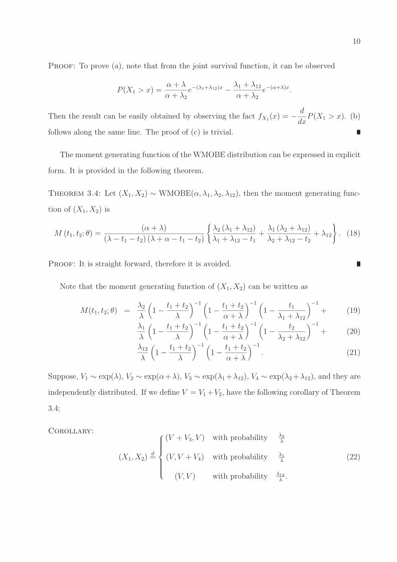
Proof: To prove (a), note that from the joint survival function, it can be observed

P (X1 > x) =α+ λ

α+ λ2

e−(λ1+λ12)x − λ1 + λ12

α+ λ2

e−(α+λ)x.

Then the result can be easily obtained by observing the fact fX1(x) = − d

dxP (X1 > x). (b)

follows along the same line. The proof of (c) is trivial.

The moment generating function of the WMOBE distribution can be expressed in explicit

form. It is provided in the following theorem.

Theorem 3.4: Let (X1, X2) ∼ WMOBE(α, λ1, λ2, λ12), then the moment generating func-

tion of (X1, X2) is

M (t1, t2; θ) =(α+ λ)

(λ− t1 − t2) (λ+ α− t1 − t2)

{λ2 (λ1 + λ12)

λ1 + λ12 − t1+λ1 (λ2 + λ12)

λ2 + λ12 − t2+ λ12

}

. (18)

Proof: It is straight forward, therefore it is avoided.

Note that the moment generating function of (X1, X2) can be written as

M(t1, t2; θ) =λ2

λ

(1 − t1 + t2

λ

)−1 (1 − t1 + t2

α+ λ

)−1 (1 − t1

λ1 + λ12

)−1

+ (19)

λ1

λ

(1 − t1 + t2

λ

)−1 (1 − t1 + t2

α+ λ

)−1 (1 − t2

λ2 + λ12

)−1

+ (20)

λ12

λ

(1 − t1 + t2

λ

)−1 (1 − t1 + t2

α+ λ

)−1

. (21)

Suppose, V1 ∼ exp(λ), V2 ∼ exp(α+λ), V3 ∼ exp(λ1 +λ12), V4 ∼ exp(λ2 +λ12), and they are

independently distributed. If we define V = V1 +V2, have the following corollary of Theorem

3.4;

Corollary:

(X1, X2)d=

(V + V3, V ) with probability λ2

λ

(V, V + V4) with probability λ1

λ

(V, V ) with probability λ12

λ.

(22)

11

Note that (22) can be used quite effectively to generate samples from the WMOBE distri-

bution. Moreover, the product moments of X1 and X2 can also be easily computed using

the representation of (22) and exponential moments, which has not attempted here.

Corollary: From the cumulant generating function (logarithm of the moment generating

function), it can be easily seen that the correlation between X1 and X2, say ρX1,X2can be

written as

ρX1,X2= (λ1 + λ12)(λ2 + λ12) ×

[1λ2 + 1

(α+λ)2− λ1λ2

(λ1+λ12)(λ2+λ12)λ2

]

√1 +

(λ1+λ12

α+λ

)2 ×√

1 +(

λ2+λ12

α+λ

)2. (23)

From (23) it is clear that for all α > 0, λ1 > 0, λ2 > 0, λ12 > 0, ρX1,X2> 0. It can be easily

seen that as α → ∞ and λ12 → 0 then ρX1,X2→ 0. Moreover, when α → ∞ and λ12 → ∞

so that λ12/α→ 0, then ρX1,X2→ 1.

Theorem 3.5: Let (X1, X2) ∼ WMOBE(α, λ1, λ2, λ12), then if λ1 = λ2, the absolute

continuous part of (X1, X2) has a total positivity of order two (TP2) property.

Proof: Note that an absolute continuous bivariate random vector, say (T1, T2) has TP2

property, if and only if for any t11, t12, t21, t22, whenever t11 < t12 and t21 < t22, we have

fT1,T2(t11, t21)fT1,T2

(t12, t22) − fT1,T2(t12, t21)fT1,T2

(t11, t22) ≥ 0, (24)

where fT1,T2(·, ·) is the joint PDF of (T1, T2). Note that by taking different ordered t11, t12, t21, t22,

such that t11 < t12 and t21 < t22, the result can be proved very easily.

4 Inference

4.1 Maximum Likelihood Estimation:

In this section we propose to compute the MLEs of the unknown parameters α, λ1, λ2, λ12

based on a random sample of size n, {(x1i, x2i), i = 1, . . . , n}. We will be using the following

12

notations.

I = {1, · · · , n}, I0 = {i ∈ I;x1i = x2i = xi}, I1 = {i ∈ I;x1i < x2i}, I2 = {i ∈ I;x1i > x2i},

and n0, n1, n2 denote the number of elements in I0, I1 and I2 respectively.

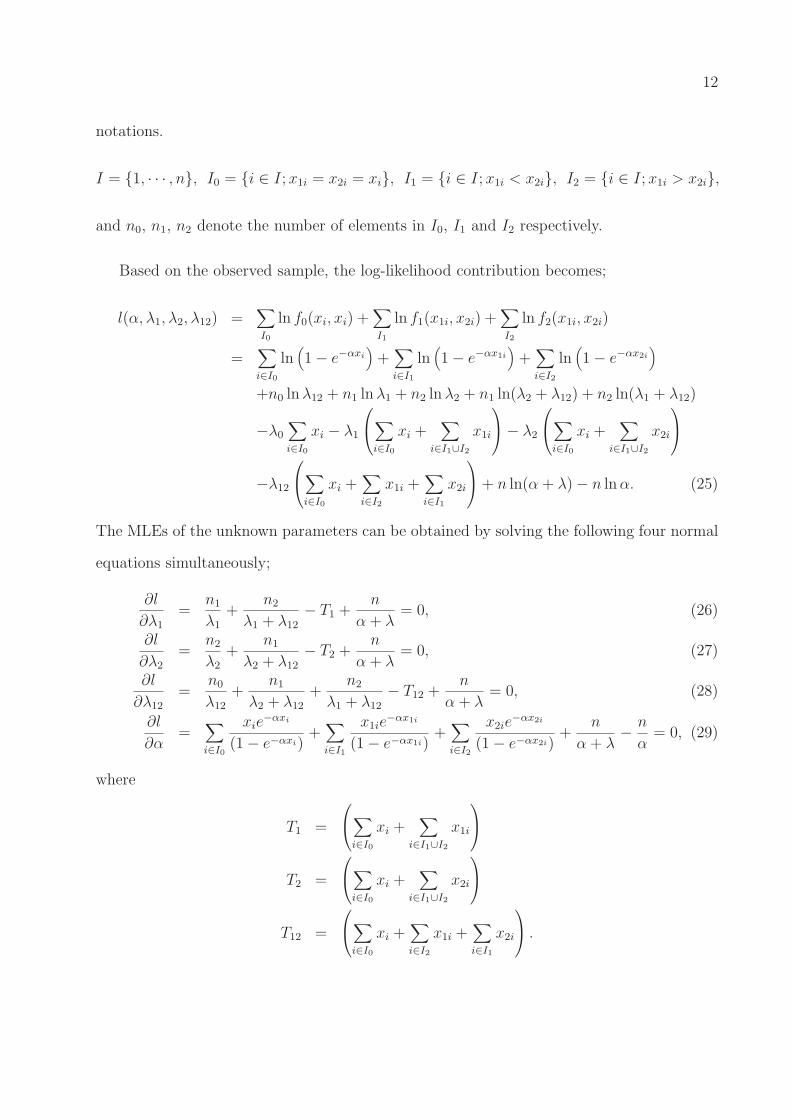
Based on the observed sample, the log-likelihood contribution becomes;

l(α, λ1, λ2, λ12) =∑

I0

ln f0(xi, xi) +∑

I1

ln f1(x1i, x2i) +∑

I2

ln f2(x1i, x2i)

=∑

i∈I0

ln(1 − e−αxi

)+∑

i∈I1

ln(1 − e−αx1i

)+∑

i∈I2

ln(1 − e−αx2i

)

+n0 lnλ12 + n1 lnλ1 + n2 lnλ2 + n1 ln(λ2 + λ12) + n2 ln(λ1 + λ12)

−λ0

∑

i∈I0

xi − λ1

∑

i∈I0

xi +∑

i∈I1∪I2

x1i

− λ2

∑

i∈I0

xi +∑

i∈I1∪I2

x2i

−λ12

∑

i∈I0

xi +∑

i∈I2

x1i +∑

i∈I1

x2i

+ n ln(α+ λ) − n lnα. (25)

The MLEs of the unknown parameters can be obtained by solving the following four normal

equations simultaneously;

∂l

∂λ1

=n1

λ1

+n2

λ1 + λ12

− T1 +n

α+ λ= 0, (26)

∂l

∂λ2

=n2

λ2

+n1

λ2 + λ12

− T2 +n

α+ λ= 0, (27)

∂l

∂λ12

=n0

λ12

+n1

λ2 + λ12

+n2

λ1 + λ12

− T12 +n

α+ λ= 0, (28)

∂l

∂α=

∑

i∈I0

xie−αxi

(1 − e−αxi)+∑

i∈I1

x1ie−αx1i

(1 − e−αx1i)+∑

i∈I2

x2ie−αx2i

(1 − e−αx2i)+

n

α+ λ− n

α= 0, (29)

where

T1 =

∑

i∈I0

xi +∑

i∈I1∪I2

x1i

T2 =

∑

i∈I0

xi +∑

i∈I1∪I2

x2i

T12 =

∑

i∈I0

xi +∑

i∈I2

x1i +∑

i∈I1

x2i

.

13

The MLEs of the unknown parameters cannot be obtained explicitly. They have to be ob-

tained by solving some numerical methods, like Newton-Raphson or Gauss-Newton methods

or their variants. Alternatively, some optimization algorithm for example genetic algorithm,

simulated annealing or down hill simplex method can be used directly to maximize the

function (25).

Initial Guess Values

To solve the above normal equations, we need to use some iterative methods and for

that we need to provide some initial guesses of the unknown parameters. Theorem 3.3 can

be used quite effectively to obtain these initial guesses. For example first we can fit WE

to X1, to get initial guesses of α + λ2 and λ1 + λ12. Similarly by fitting WE to X2 and to

min{X1, X2}, we can obtain initial guesses of α + λ1, λ2 + λ12, α and λ. From these initial

guesses we can obtain initial guesses of all the unknown parameters easily.

Asymptotic Properties

Although, the proposed WMOBE distribution is a singular distribution, but it can be

shown along the same line as the MOBE model that the asymptotic distribution of the MLEs

is multivariate normal. The result is given below without proof.

Theorem 4.1 As n → ∞, the MLEs of θ, say θ̂ = (α̂, λ̂1, λ̂2, λ̂12) has the following asymp-

totic property;√n{(α̂, λ̂1, λ̂2, λ̂12) − (α, λ1, λ2, λ12)

}−→ N4(0, I

−1),

here I is the expected Fisher information matrix, and the exact expression of I is provided

in Appendix B.

14

4.2 Testing of Hypothesis

It is already mentioned that the MOBE distribution is a limiting member of the class of

WMOBE distributions. In this subsection only let us denote β =1

α. With the abuse

of notation, let us denote the new parameter space also as θ = (β, λ1, λ2, λ12), where

β > 0, λ1 > 0, λ2 > 0, λ12 ≥ 0. When β = 0, it corresponds to the MOBE model. So

one of the natural testing of hypothesis problem will be to test the following:

H0 : β = 0, vs H1 : β > 0. (30)

In this case since β is in the boundary under the null hypothesis, the standard results do

not work. But using Theorem 3 of Self and Liang [16], it follows that

2(lWMOBE(β̂, λ̂1, λ̂2, λ̂12) − lMOBE(λ̂1, λ̂2, λ̂12)) −→1

2+

1

2χ2

1.

Here lWMOBE(·) and lMOBE(·) denote the log-likelihood functions at the maximum likelihood

values of WMOBE and MOBE models respectively.

5 Data Analysis

American Football Data Set: This data set is obtained from the American Football

(National Football League) League from the matches on three consecutive weekends in 1986.

The data were first published in ‘Washington Post’, and they are available in Csorgo and

Welsch [7]. The ‘seconds’ in the data have been converted to the decimal points, as it has

been done by Csorgo and Welsch [7], and they are presented in Table 1. In this bivariate

data set (X1, X2), the variable X1 represents the game time to the first points scored by

kicking the ball between goal posts and X2 represents the ‘game time’ by moving the ball

into the end zone.

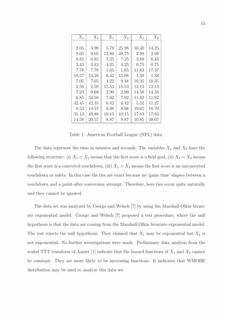
15

X1 X2 X1 X2 X1 X2

2.05 3.98 5.78 25.98 10.40 14.259.05 9.05 13.80 49.75 2.98 2.980.85 0.85 7.25 7.25 3.88 6.433.43 3.43 4:25 4.25 0.75 0.757.78 7.78 1.65 1.65 11.63 17.37

10.57 14.28 6.42 15.08 1.38 1.387.05 7.05 4.22 9.48 10.35 10.352.58 2.58 15.53 15.53 12.13 12.137.23 9.68 2.90 2.90 14.58 14.586.85 34.58 7.02 7.02 11.82 11.82

32.45 42.35 6.42 6.42 5.52 11.278.53 14.57 8.98 8.98 19.65 10.70

31.13 49.88 10.15 10.15 17.83 17.8314.58 20.57 8.87 8.87 10.85 38.07

Table 1: American Football League (NFL) data

The data represent the time in minutes and seconds. The variables X1 and X2 have the

following structure: (i) X1 < X2 means that the first score is a field goal, (ii) X1 = X2 means

the first score is a converted touchdown, (iii) X1 > X2 means the first score is an unconverted

touchdown or safety. In this case the ties are exact because no ‘game time’ elapses between a

touchdown and a point-after conversion attempt. Therefore, here ties occur quite naturally

and they cannot be ignored.

The data set was analyzed by Csorgo and Welsch [7] by using the Marshall-Olkin bivari-

ate exponential model. Csorgo and Welsch [7] proposed a test procedure, where the null

hypothesis is that the data are coming from the Marshall-Olkin bivariate exponential model.

The test rejects the null hypothesis. They claimed that X1 may be exponential but X2 is

not exponential. No further investigations were made. Preliminary data analysis from the

scaled TTT transform of Aarset [1] indicate that the hazard functions of X1 and X2 cannot

be constant. They are more likely to be increasing functions. It indicates that WMOBE

distribution may be used to analyze this data set.

16

It should further be noted that the possible scoring times are restricted by the duration

of the game but it has been ignored similarly as in Csorgo and Welsh [7]. Here all the data

points are divided by 10 just for computational purposes. It should not make any difference

in the statistical inference.

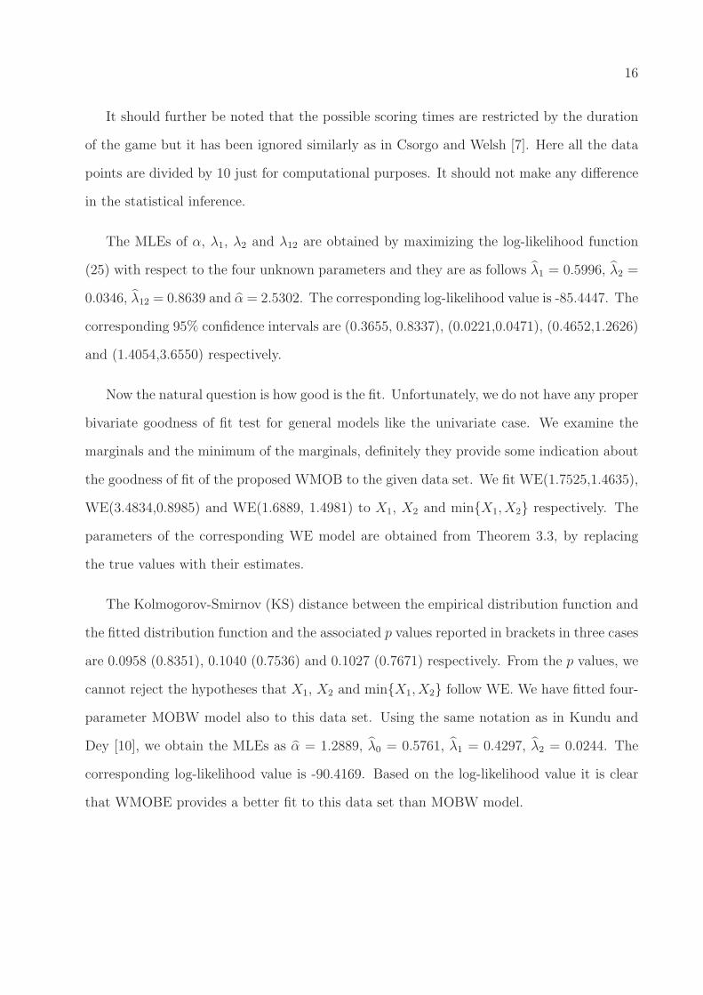
The MLEs of α, λ1, λ2 and λ12 are obtained by maximizing the log-likelihood function

(25) with respect to the four unknown parameters and they are as follows λ̂1 = 0.5996, λ̂2 =

0.0346, λ̂12 = 0.8639 and α̂ = 2.5302. The corresponding log-likelihood value is -85.4447. The

corresponding 95% confidence intervals are (0.3655, 0.8337), (0.0221,0.0471), (0.4652,1.2626)

and (1.4054,3.6550) respectively.

Now the natural question is how good is the fit. Unfortunately, we do not have any proper

bivariate goodness of fit test for general models like the univariate case. We examine the

marginals and the minimum of the marginals, definitely they provide some indication about

the goodness of fit of the proposed WMOB to the given data set. We fit WE(1.7525,1.4635),

WE(3.4834,0.8985) and WE(1.6889, 1.4981) to X1, X2 and min{X1, X2} respectively. The

parameters of the corresponding WE model are obtained from Theorem 3.3, by replacing

the true values with their estimates.

The Kolmogorov-Smirnov (KS) distance between the empirical distribution function and

the fitted distribution function and the associated p values reported in brackets in three cases

are 0.0958 (0.8351), 0.1040 (0.7536) and 0.1027 (0.7671) respectively. From the p values, we

cannot reject the hypotheses that X1, X2 and min{X1, X2} follow WE. We have fitted four-

parameter MOBW model also to this data set. Using the same notation as in Kundu and

Dey [10], we obtain the MLEs as α̂ = 1.2889, λ̂0 = 0.5761, λ̂1 = 0.4297, λ̂2 = 0.0244. The

corresponding log-likelihood value is -90.4169. Based on the log-likelihood value it is clear

that WMOBE provides a better fit to this data set than MOBW model.

17

Now we want to perform the testing of hypothesis problem as defined in (30). We have

fitted three-parameter MOBE model to this data set, and obtain the estimates of λ0, λ1

and λ2 (using the same notations as in Kundu and Dey [10]) as 0.7145, 0.4562 and 0.0298

respectively. The log-likelihood value is -93.3058, and the p value of the test statistic is less

than 0.0001. Therefore, we reject the null hypothesis that the data are coming from a MOBE

distribution.

6 Conclusions

In this paper we have proposed a new singular bivariate distribution whose marginals are

weighted exponential distribution recently proposed by Gupta and Kundu [9]. This singular

distribution has been obtained as a hidden truncation model as of Azzalini [5]. This new four-

parameter bivariate exponential distribution has explicit probability density function and

the distribution function. We have derived several interesting properties of this distribution.

Marshall-Olkin bivariate exponential distribution can be obtained as a limiting distribution

of this model. It is observed that in some cases it may provide a better fit than the existing

well known MOBE or MOBW models.

It may be mentioned that although in this paper we have proposed bivariate weighted

exponential model, but similarly, weighted Marshall-Olkin multivariate exponential distri-

bution also can be defined. Moreover, along the same line the weighted Marshall-Olkin

bivariate or multivariate Weibull distribution also can be introduced. More work is needed

in these direction.

18

Acknowledgements:

The authors would like to thank the two referees for their valuable suggestions which has

helped them to improve the manuscript significantly. Part of this work has been supported

by a grant from the Department of Science and Technology, Government of India.

References

[1] Aarset, M.V. (1987), “How to identify a bathtub hazard rate?”, IEEE Transactions on

Reliability, vol. 36, 106 - 108.

[2] Al-Mutairi, D.K., Ghitany, M.E. and Kundu, D. (2011), “A new bivariate distribution

with weighted exponential marginals and its multivariate generalization”, Statistical

Papers, to appear.

[3] Arnold, B. C. and Beaver, R. J. (2000), “Hidden truncation model”, Sankhya, Ser. A,

vol. 62, 23 - 35.

[4] Arnold, B.C. and Beaver, R. J. (2002), “Selective multivariate models related to hidden

truncation and/ or selective reporting”, Test, vol. 11, 7 - 54.

[5] Azzalini, A. (1985), “A class of distributions which includes the normal ones”, Scandi-

navian Journal of Statistics, vol. 12, 171 - 185.

[6] Bemis, B., Bain, L.J. and Higgins, J.J. (1972), “Estimation and hypothesis testing

for the parameters of a bivariate exponential distribution”, Journal of the American

Statistical Association, vol. 67, 927 -929.

[7] Csorgo, S. and Welsh, A.H. (1989), “Testing for exponential and Marshall-Olkin distri-

bution”, Journal of Statistical Planning and Inference, vol. 23, 287 - 300.

19

[8] Genton, M. G. (ed.) (2004), Skew-Elliptical Distributions and their Applications: A

Journey Beyond Normality, Chapman and Hall/CRS, New York.

[9] Gupta, R. D. and Kundu, D. (2009), “A new class of weighted exponential distribu-

tions”, Statistics, to appear, DOI: 10.1080/02331880802605346.

[10] Kundu, D. and Dey, A.K. (2009), “Estimating the parameters of the Marshall Olkin

bivariate Weibull distribution by EM algorithm”, Computational Statistics and Data

Analysis, vol. 53, no. 4, 956 - 965.

[11] Kundu, D. and Gupta, R.D. (2009), “Bivariate generalized exponential distribution”,

Journal of Multivariate Analysis, vol. 100, 581 - 593.

[12] Kotz, S., Johnson, N.L. and Balakrishnan, N. (2000), Continuous Multivariate Dis-

tributions, vol. 1, Models and Applications, 2nd-edition, John Wiley and Sons, New

York.

226 - 233.

[13] Meintanis, S.G. (2007), “Test of fit for Marshall-Olkin distributions with applications”,

Journal of Statistical Planning and Inference, vol. 137, 3954 - 3963.

[14] Press, W.H., Teukolsky, S.A., Vellerling, W.T. and Flannery, B.P. (1992), Numerical

Recipes in FORTRAN, The Art of Scientific Computing, 2nd. ed., Cambridge University,

Cambridge, U.K.

[15] Sarhan, A. and Balakrishnan, N. (2007), “A new class of bivariate distribution and its

mixtures”, Journal of Multivariate Analysis, vol. 98, 1508 - 1527.

[16] Self, S.G. and Liang, K-L., (1987), “Asymptotic properties of the maximum likelihood

estimators and likelihood ratio test under non-standard conditions”, Journal of the

American Statistical Association, vol. 82, 605 - 610.

20

Appendix: Expected Fisher Information Matrices

Let the Fisher information matrix be;

I = −E

∂2l∂α2

∂2l∂α∂λ1

∂2l∂α∂λ2

∂2l∂α∂λ12

∂2l∂λ1∂α

∂2l∂λ2

1

∂2l∂λ1∂λ2

∂2l∂λ1∂λ12

∂2l∂λ2∂α

∂2l∂λ2λ1

∂2l∂λ2

2

∂2l∂λ2∂λ12

∂2l∂λ12∂α

∂2l∂λ12λ1

∂2l∂λ12λ2

∂2l∂λ2

12

. (31)

Now we provide all the elements of the Fisher information matrix, and for that we need the

following results;

P (X1 < X2) =λ1

λ, P (X1 > X2) =

λ2

λ, P (X1 = X2) =

λ12

λ,

moreover, we will be using the following notation;

ψ(α, λ) =α+ λ

λ

∫ ∞

0

x2e−(α+λ)x

(1 − e−αx)dx.

E

[∂2l

∂α2

]

= −E

n

(α+ λ)2− n

α2+∑

i∈I1

X21ie

−λX1i

(1 − e−αX1i)2+∑

i∈I2

X22ie

−λX2i

(1 − e−αX2i)2+∑

i∈I0

X2i e

−λXi

(1 − e−αXi)2

= −n[

1

(α+ λ)2− 1

α2+ψ(α, λ)

λ

(λ2

1 + λ22 + λ2

12

)]

E

[∂2l

∂λ21

]

= −E[n1 + n2

λ21

+n

(α+ λ)2+

n2

(λ1 + λ12)2

]

= −n[λ1 + λ2

λλ21

+1

(α+ λ)2+

λ2

λ(λ1 + λ12)2

]

E

[∂2l

∂λ22

]

= −E[n1 + n2

λ22

+n

(α+ λ)2+

n1

(λ1 + λ12)2

]

= −n[λ1 + λ2

λλ21

+1

(α+ λ)2+

λ2

λ(λ1 + λ12)2

]

E

[∂2l

∂λ212

]

= −E[

n1

(λ2 + λ12)2+

n2

(λ1 + λ12)2+

n

(α+ λ)2+n0

λ212

]

= −n[

λ1

λ(λ2 + λ12)2+

λ2

λ(λ1 + λ12)2+

1

(α+ λ)2+

1

λλ12

]

21

E

[∂2l

∂α∂λ1

]

= E

[∂2l

∂α∂λ2

]

= E

[∂2l

∂α∂λ12

]

= E

[∂2l

∂λ1∂λ2

]

= − n

(α+ λ)2

E

[∂2l

∂λ1∂λ12

]

= −E[

n2

(λ1 + λ12)2+

n

(α+ λ)2

]

= −n[

λ2

λ(λ1 + λ12)2+

1

(α+ λ)2

]

E

[∂2l

∂λ2∂λ12

]

= −E[

n1

(λ2 + λ12)2+

n

(α+ λ)2

]

= −n[

λ1

λ(λ2 + λ12)2+

1

(α+ λ)2

]

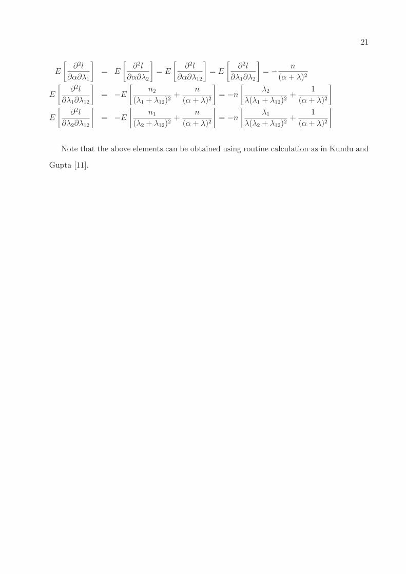
Note that the above elements can be obtained using routine calculation as in Kundu and

Gupta [11].

22

0 0.5

1 1.5

2 2.5 0

0.5 1

1.5 2

2.5

0 0.1 0.2 0.3 0.4 0.5 0.6 0.7 0.8

(a)

0 0.5

1 1.5

2 2.5 0

0.5 1

1.5 2

2.5

0 0.1 0.2 0.3 0.4 0.5 0.6 0.7 0.8

(b)

0 0.5

1 1.5

2 2.5 0

0.5 1

1.5 2

2.5

0 0.2 0.4 0.6 0.8

1 1.2

(c)

0 0.2 0.4 0.6 0.8 1 1.2 1.4 0 0.2

0.4 0.6

0.8 1

1.2 1.4

0 0.2 0.4 0.6 0.8

1 1.2 1.4 1.6

(d)

Figure 1: The surface plot of the absolute continuous part of the joint PDF of (12) whenλ1 = λ2 = λ12 = 1 and (a) α = 0.001, (b) α = 0.5, (c) α = 5, and (d) α = 25.