Marshall-Olkin Beta Distribution and its Applicationsshodhganga.inflibnet.ac.in/bitstream/10603/22815/10/10_chapter2.pdf · CHAPTER 2 Marshall-Olkin Beta Distribution and its Applications

CHAPTER 2

Marshall-Olkin Beta Distribution and its

Applications

2.1 Introduction

The majority of continuous distributions are defined on infinite intervals. But beta distribu-

tion is a continuous distribution defined on a bounded interval and its probability density

function exhibits a wide range of shapes. This flexibility encourages its empirical use in a

large variety of applications. For many years the use of beta distribution has been as ‘prior’

distribution for binomial proportions. In recent years beta distributions have been used in

modelling distributions of hydrological variables, in operation research, in risk analysis etc.

See Nadarajah (2007a) for some references.

Recently many authors have obtained generalizations of beta distribution using various

Some results included in this chapter have appeared in the paper Jose et al. (2009)

25

CHAPTER 2. MARSHALL-OLKIN BETA DISTRIBUTION AND ITS APPLICATIONS

techniques. McDonald and Xu (1995) introduced a five-parameter beta distribution. Var-

ious properties of a family of generalized beta distributions including beta-normal, beta-

exponential, beta-Weibull etc are recently studied by different authors. Sepanski and Kong

(2007) applied these distributions to the modelling of the size distribution of income and

computed the maximum likelihood estimates of parameters. They also compared these

estimates with those of the widely used generalized beta distributions of the first and sec-

ond kind in terms of measures of goodness of fit.

New parameters can be introduced to expand families of distributions for added flex-

ibility. In this paper we generalize the beta distribution using the method proposed by

Marshall and Olkin (1997). They introduced a method of obtaining a family of distributions

given by

G(x) =F (x)

α+ (1− α)F (x), x ∈ R (2.1.1)

where F is a distribution function and α > 0. If α = 1 then we have G = F . The

distribution function G has the density given by

g(x) =αf(x)

(α+ (1− α)F (x))2

and the hazard rate

r(x) =rF (x)

α+ (1− α)F (x),

where rF (x) is the hazard rate of the distribution function F . In the past decade, many dis-

tributions which belong to the Marshall-Olkin family of distributions have been investigated.

Marshall and Olkin (1997) defined exponential and Weibull. Alice and Jose (2003), (2004)

(2005a) and (2005b) introduced and studied the various properties of semi-Weibull, bi-

variate semi-Pareto, Pareto and logistic distributions. Marshall-Olkin q-Weibull distribution

was introduced by Jose, Naik and Ristic (2008) and they discussed its application in time

series modelling. Semi-Burr distribution was studied by Jayakumar and Thomas (2007).

A physical interpretation of the Marshall-Olkin model using odds function was given by

Sankaran and Jayakumar (2007).

26


By a minification process of order 1 we mean a sequence {Xn, n ≥ 0} of nonnegative

random variables having the structure

Xn = kmin(Xn−1, εn), n ≥ 1

where {εn} is a sequence of independent and identically distributed (i.i.d) random variables

called innovations and k > 1. The study on autoregressive processes having minification

structure began with the work of Tavares (1980) and subsequently many authors devel-

oped minification processes with different marginal distributions. See Sim (1986), (1994),

Yeh et al. (1988), Lewis and Mckenzie (1991) and Pillai (1991). Balakrishna and Jacob

(2003) discussed the parameter estimation of a univariate minification process and stud-

ied properties such as ergodicity and uniform mixing. Ed Mckenzie (1985) presented two

stationary first order autoregressive processes with beta marginal distributions.

In section 2 the Marshall-Olkin beta distribution is introduced and some shape prop-

erties are discussed. In section 3 maximum likelihood estimation of the parameters are

considered. The expression for the moments are derived in section 4. In section 5 a minifi-

cation process with Marshall-Olkin beta distribution is introduced and some of its properties

are obtained. In section 6 two real data sets are analyzed and the new distribution is found

a better fit than the standard beta distribution.

2.2 A Marshall-Olkin Beta Distribution and its Properties

In this section we introduce a Marshall-Olkin beta distribution. Let

F (x) =B

(m,n, x−a

b−a

)B(m,n)

=1

B(m,n)

∫ x−ab−a

0

tm−1(1− t)n−1dt, a < x < b,

be the distribution function of a beta distribution with parameters m > 0, n > 0, a and b.

Replacing F in (2.1.1) we obtain the distribution function of a Marshall-Olkin beta distribu-

tion as

G(x) =B

(m,n, x−a

b−a

)αB(m,n) + (1− α)B

(m,n, x−a

b−a

) . (2.2.1)

27


The corresponding probability density function has the form

g(x) =αB(m,n)(x− a)m−1(b− x)n−1

(b− a)m+n−1(αB(m,n) + (1− α)B

(m,n, x−a

b−a

))2 .

The Marshall-Olkin beta distribution with parameters m, n, a, b and α is denoted by MO-

Beta (m,n, a, b, α). If α = 1 then the MOBeta (m,n, a, b, α) distribution reduces to the

four parameter beta distribution.

If m and n are positive integers, then the distribution function G is given by

G(x) =

m+n−1∑r=m

(m+n−1

r

)(x− a)r(b− x)m+n−r−1

α(b− a)m+n−1 + (1− α)m+n−1∑

r=m

(m+n−1

r

)(x− a)r(b− x)m+n−r−1

and the probability density function has the form

g(x) =α(b− a)m+n−1(x− a)m−1(b− x)n−1

B(m,n)

(α(b− a)m+n−1 + (1− α)

m+n−1∑r=m

(m+n−1

r

)(x− a)r(b− x)m+n−r−1

)2 .

Now we discuss some shape properties of the MOBeta (m,n, a, b, α) distribution. The

parameters m, n and α are the shape parameters. The first derivative of log g(x) is

d log g(x)

dx=

t(x)

(b− a)m+n−1(x− a)(b− x)(αB(m,n) + (1− α)B

(m,n, x−a

b−a

)) ,where

t(x) = −2(1− α)(x− a)m(b− x)n + [(m− 1)b+ (n− 1)a− (m+ n− 2)x]

×(b− a)m+n−1

(αB(m,n) + (1− α)B

(m,n,

x− a

b− a

)).

The following cases are possible:

1. If 0 < m,n < 1, then t(x) is an increasing function with unique root x0. Thus it

28


follows that g(x) decreases at (a, x0] and increases at (x0, b) with g(a) = g(b) = ∞.

2. Let 0 < n < 1 < m and α < 1.

(a) If m + n > 2 and t(x) has two real roots x1 and x2, then t(x) is positive at

(a, x1] ∪ (x2, b) and negative at (x1, x2]. Thus it follows that g(x) increases at

(a, x1] ∪ (x2, b) and decreases at (x1, x2] with g(a) = 0 and g(b) = ∞.

(b) If m+ n < 2, t′(x) and t(x) have two real roots, where x1 and x2 are the roots

of t(x), then g(x) has the same shape as in 2(a).

(c) Otherwise, g(x) is an increasing function with g(a) = 0 and g(b) = ∞.

3. If 0 < n < 1 < m and α > 1, then t(x) is a positive function. Thus it follows that

g(x) is an increasing function with g(a) = 0 and g(b) = ∞.

4. If 0 < m < 1 < n and α < 1, then t(x) is a negative function. Thus it follows that

g(x) is a decreasing function with g(a) = ∞ and g(b) = 0.

5. Let 0 < m < 1 < n and α > 1.

(a) If m + n > 2 and t(x) has two real roots x1 and x2, then t(x) is negative at

(a, x1] ∪ (x2, b) and positive at (x1, x2]. Thus it follows that g(x) decreases at

(a, x1] ∪ (x2, b) and increases at (x1, x2] with g(a) = ∞ and g(b) = 0.

(b) If m+ n < 2, t′(x) and t(x) have two real roots, where x1 and x2 are the roots

of t(x), then g(x) has the same shape as in 5(a).

(c) Otherwise, g(x) is an decreasing function with g(a) = ∞ and g(b) = 0.

6. If m,n > 1, then t(x) is a decreasing function with unique root x0. Thus it follows

that g(x) is a unimodal function with mode at x0 and g(a) = g(b) = 0.

Now, we define the hazard rate function. The hazard rate function of the Marshall-Olkin

beta distribution is given by

r(x) =B(m,n)(x− a)m−1(b− x)n−1(

αB(m,n) + (1− α)B(m,n, x−a

b−a

)) (B(m,n)−B

(m,n, x−a

b−a

))29


Figure 2.1: Graph of the probability density function of the Marshall-Olkin beta distribution fora = 0, b = 1 and various values of the parameters m, n and α.

Now we establish some properties of the Marshall-Olkin beta distribution.

Theorem 2.2.1. Let {Xn, n ≥ 1} be a sequence of i.i.d. random variables with a

MOBeta(m,n, a, b, α) distribution. Let N be a geometric r.v. with parameter p and

suppose that N and Xi are independent. Then:

i) min(X1, X2, . . . , XN) has a MOBeta(m,n, a, b, αp) distribution.

ii) max(X1, X2, . . . , XN) has a MOBeta(m,n, a, b, α/p) distribution.

Proof. : (i) Survival function of U = min(X1, X2, . . . , XN) is given by

P (U > u) = p

∞∑s=1

[G(u)

]s(1− p)s−1

=αpB

(n,m, b−u

b−a

)αpB(m,n) + (1− αp)B

(m,n, u−a

b−a

) .This is the survival function of a MOBeta (m,n, a, b, αp) distribution.

30


Figure 2.2: Graph of the hazard rate function of the Marshall-Olkin beta distribution for a = 0,b = 1 and different values of the parameters m, n and α.

(ii) To prove this consider the distribution function of Xn given by (2.2.1).

Let V = max(X1, X2, . . . , XN). Then distribution function of V is given by

P (V ≤ v) = p∞∑

s=1

[G(v)]s (1− p)s−1

=B

(m,n, v−a

b−a

)αpB(m,n) +

(1− α

p

)B

(m,n, v−a

b−a

)This is a MOBeta (m,n, a, b, α/p) distribution.

Corollary 2.2.1. Let {Xn} be a sequence of i.i.d. random variables with a beta dis-

tribution with parameters m, n, a and b. Let N be a Geometric(p) r.v. and suppose

that N and Xi are independent. Then:

i) min(X1, X2, . . . , XN) has a MOBeta(m,n, a, b, p) distribution.

ii) max(X1, X2, . . . , XN) has a MOBeta(m,n, a, b, 1/p) distribution.

31


2.3 Estimation

We consider estimation of the unknown parameters by the method of maximum likelihood.

The log-likelihood function for some realizations x1, x2, . . . , xN is

logL(m,n, a, b, α) = N logα+N logB(m,n) + (m− 1)N∑

i=1

log(xi − a)

+(n− 1)N∑

i=1

log(b− xi)−N(m+ n− 1) log(b− a)

−2N∑

i=1

log

(αB(m,n) + (1− α)B

(m,n,

xi − a

b− a

)).

The first derivatives of logL(m,n, a, b, α) with respect to m, n, a, b and α are

∂ logL

∂m= N(ψ(m)− ψ(m+ n)) +

N∑i=1

log(xi − a)−N log(b− a)

−2N∑

i=1

1

αB(m,n) + (1− α)B(m,n, xi−a

b−a

)[αB(m,n)(ψ(m)− ψ(m+ n))

+(1− α)

(B

(m,n,

xi − a

b− a

)log

(xi − a

b− a

)−

(xi − a

b− a

)m

Γ2(m)

× 3F2

(m,m, 1− n;m+ 1,m+ 1;

xi − a

b− a

))]∂ logL

∂n= N(ψ(n)− ψ(m+ n)) +

N∑i=1

log(b− xi)−N log(b− a)

−2N∑

i=1

1


b−a

)[B(m,n)(ψ(n)− ψ(m+ n))

+(1− α)

(Γ2(n)

(b− xi

b− a

)n

3F2

(n, n, 1−m;n+ 1, n+ 1;

b− xi

b− a

)− log

(b− xi

b− a

)B

(n,m,

b− xi

b− a

)) ]

32


∂ logL

∂a= (1−m)

N∑i=1

1

xi − a+N(m+ n− 1)

b− a+

2(1− α)

(b− a)m+n

×N∑

i=1

(xi − a)m−1(b− xi)n


b−a

)∂ logL

∂b= (n− 1)

N∑i=1

1

b− xi

− N(m+ n− 1)

b− a+

2(1− α)

(b− a)m+n

×N∑

i=1

(xi − a)m(b− xi)n−1


b−a

)∂ logL

∂α=

N

α− 2

N∑i=1

B(n,m, b−xi

b−a

)αB(m,n) + (1− α)B

(m,n, xi−a

b−a

)where

3F2(a1, a2, a3; b1, b2; z) =1

Γ(b1)Γ(b2)

∞∑k=0

(a1)k(a2)k(a3)k

(b1)k(b2)k

· zk

k!.

The maximum likelihood estimates can be obtained setting the above expressions to zero

and solving them numerically. Function nlm from the statistical software R can be used for

finding the maximum likelihood estimates.

2.4 Moments

We derive the moments of a random variable X with MOBeta(m,n, 0, 1, p) distribution,

since if X d= MOBeta(m,n, 0, 1, p) then Y = a + (b − a)X has a MOBeta(m,n, a, b, p)

distribution. Let us first consider the case p < 1. Let X1,N = min(X1, X2, . . . , XN).

From Corollary(2.2.1) it follows that X d= X1,N . Then the kth order moment of the random

variable X is

E(Xk) = E(Xk1,N) = p

∞∑r=1

(1− p)r−1E(Xk1,r), (2.4.1)

where X1,r = min(X1, X2, . . . , Xr). Nadarajah (2007b) derived the kth order moments of

beta order statistics as

33


E(Xk1,r) = r

r−1∑l=0

(−1)l

(r − 1

l

)B(n, k +m(l + 1))

ml(B(m,n))l+1

∞∑m1=0

· · ·

∞∑ml=0

(k +m(l + 1))m1+···+ml(1− n)m1(m)m1 · · · (1− n)ml

(m)ml

(n+ k +m(l + 1))m1+···+ml(m+ 1)m1 · · · (m+ 1)ml

m1! . . .ml!(2.4.2)

where (k)s is the ascending factorial defined as (k)s = k(k+1) . . . (k+s−1) with (k)0 = 1.

Combining (2.4.1) and (2.4.2), we obtain the expression

E(Xk) = p∞∑

r=1

r(1− p)r−1

r−1∑l=0

(−1)l

(r − 1

l

)B(n, k +m(l + 1))

ml(B(m,n))l+1

∞∑m1=0

· · ·

∞∑ml=0

(k +m(l + 1))m1+···+ml(1− n)m1(m)m1 · · · (1− n)ml

(m)ml

(n+ k +m(l + 1))m1+···+ml(m+ 1)m1 · · · (m+ 1)ml

m1! . . .ml!.

Let us consider the case p ≥ 1. LetXN,N = max(X1, X2, . . . , XN). From Corollary (2.2.1)

it follows that X d= XN,N . Then the kth order moment of the random variable X is

E(X) = E(XkN,N) =

1

p

∞∑r=1

(1− 1

p

)r−1

E(Xkr,r), (2.4.3)

where Xr,r = max(X1, X2, . . . , Xr). Using Nadarajah (2007b) and (2.4.3), we obtain the

expression

E(Xk) =1

p

∞∑r=1

r

(1− 1

p

)r−1B(n, k +mr)

mr−1(B(m,n))r

∞∑m1=0

· · ·

∞∑mr−1=0

(k +mr)m1+···+mr−1(1− n)m1(m)m1 · · · (1− n)mr−1(m)mr−1

(n+ k +mr)m1+···+mr−1(m+ 1)m1 · · · (m+ 1)mr−1m1! . . .mr−1!.

A program written in R which can be used to compute the moments of a random variable

with MOBeta(m,n, 0, 1, α) distribution is presented in Appendix.

34


2.5 A Marshall-Olkin Beta Minification Process

We introduce a minification process with MOBeta (m,n, a, b, α) distribution. Consider a

process {Xn, n ≥ 1} given by

Xn =

εn, w.p α

min(Xn−1, εn), w.p 1− α(2.5.1)

where {εn, n ≥ 1} is a sequence of i.i.d. random variables, Xn−1 and εn are independent

random variables and 0 < α < 1. Suppose that {εn, n ≥ 1} is a sequence of i.i.d.

random variables with beta distribution with parametersm, n, a, b and letX0 has a MOBeta

(m,n, a, b, α) distribution. Then it follows from (2.2.1) and (2.5.1) that

FX1(x) = αF ε(x) + (1− α)FX0(x)F ε(x) =αB

(n,m, b−x

b−a

)αB(m,n) + (1− α)B

(m,n, x−a

b−a

) .Thus it follows thatX1 has a MOBeta(m,n, a, b, α) distribution. Then by induction it follows

that Xn has the same distribution. Thus {Xn, n ≥ 0} is a stationary process with MOBeta

(m,n, a, b, α) distribution. Conversely suppose that {Xn, n ≥ 0} is a stationary process

with a MOBeta(m, n, a, b, α) distribution. Also let {εn, n ≥ 1} be a sequence of i.i.d.

random variables. Then

F ε(x) =FX(x)

α+ (1− α)FX(x)=B

(n,m, b−x

b−a

)B(m,n)

.

Therefore {εn, n ≥ 1} has a beta distribution with parameters m, n, a and b. Thus we

have proved the following result.

Theorem 2.5.1. Let {εn, n ≥ 1} is a sequence of i.i.d. random variables. A random

process {Xn, n ≥ 0} given by (2.5.1) is a stationary process with MOBeta(m, n, a, b, α)

distribution if and only if εn has a beta distribution with parameters m, n, a and b.

Let us consider some properties of the Marshall-Olkin beta minification process. First

35


we derive the joint survival function of a random vector (Xn+1, Xn) as

FXn+1,Xn(x, y) = P [Xn+1 > x,Xn > y]

= F ε(x)[αFX(y) + (1− α)FX(max(x, y))]

=

αB(n,m, b−x

b−a)B(n,m, b−yb−a)

B(m,n)(αB(m,n)+(1−α)B(m,n, y−ab−a ))

, x < y

αB(n,m, b−xb−a)

B(m,n)

[B(m,n)

αB(m,n)+(1−α)B(m,n, x−ab−a )

− B(m,n, y−ab−a )

αB(m,n)+(1−α)B(m,n, y−ab−a )

], x > y.

This survival function is not absolutely continuous since

P (Xn+1 = Xn) =1− α+ α logα

1− α∈ (0, 1).

The above probability is a decreasing function of α.

The probability of the event {Xn+1 > Xn} can be obtained as

P (Xn+1 > Xn) =α(1− α+ α logα)

(1− α)2∈ (0, 0.5).

The above probability is an increasing function of α.

2.6 Auto-Covariance Structure

Let us consider the autocovariance between the random variables Xn+1 and Xn. Let

µk = E(Xk) be the kth order moment of the random variableX with MOBeta(m,n, a, b, α)

distribution. We have that

Cov(Xn+1, Xn) = (1− α)Cov(min(Xn, εn+1), Xn).

From (2.5.1), E(Xn) = µ1 and E(εn+1) = (bm+ an)/(m+ n), so that

E(min(Xn, εn+1)) =(m+ n)µ1 − α(bm+ an)

(1− α)(m+ n).

36


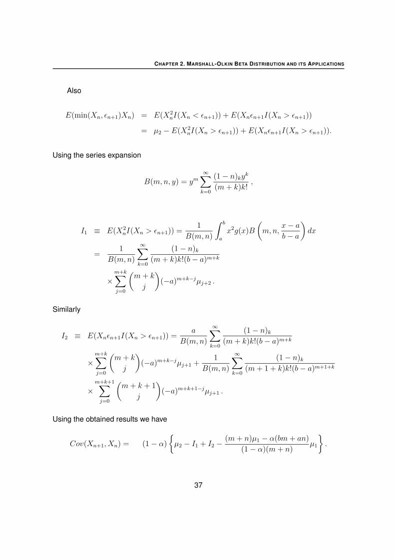
Also

E(min(Xn, εn+1)Xn) = E(X2nI(Xn < εn+1)) + E(Xnεn+1I(Xn > εn+1))

= µ2 − E(X2nI(Xn > εn+1)) + E(Xnεn+1I(Xn > εn+1)).

Using the series expansion

B(m,n, y) = ym

∞∑k=0

(1− n)kyk

(m+ k)k!,

I1 ≡ E(X2nI(Xn > εn+1)) =

1

B(m,n)

∫ b

a

x2g(x)B

(m,n,

x− a

b− a

)dx

=1

B(m,n)

∞∑k=0

(1− n)k

(m+ k)k!(b− a)m+k

×m+k∑j=0

(m+ k

j

)(−a)m+k−jµj+2 .

Similarly

I2 ≡ E(Xnεn+1I(Xn > εn+1)) =a

B(m,n)

∞∑k=0

(1− n)k

(m+ k)k!(b− a)m+k

×m+k∑j=0

(m+ k

j

)(−a)m+k−jµj+1 +

1

B(m,n)

∞∑k=0

(1− n)k

(m+ 1 + k)k!(b− a)m+1+k

×m+k+1∑

j=0

(m+ k + 1

j

)(−a)m+k+1−jµj+1 .

Using the obtained results we have

Cov(Xn+1, Xn) = (1− α)

{µ2 − I1 + I2 −

(m+ n)µ1 − α(bm+ an)

(1− α)(m+ n)µ1

}.

37


Table 2.1: Estimated values, log-likelihood and Kolmogorov-Smirnov statistics for dataset 1

.

Distribution Estimates − log L K-SBeta m = 0.8005 360.9736 0.0832

n = 1.2346a = 191

b = 980.9115Marshall-Olkin beta m = 1.5507 356.7594 0.0534

n = 0.4641a = 188.261

b = 975α = 0.0925

2.7 Data Analysis

In this section we analyze some data sets and compare Marshall-Olkin beta distribution

with beta distriution.

Data Set 1. First we start with the data used in Ricciardi (2005). The data represent

permeability values from three horizons of the Dominquez field of Southern California.

Permeability data measured in millidarcies are: 292, 346, 403, 640, 191, 353, 447, 696,

251, 390, 498, 615, 248, 370, 424, 650, 241, 370, 523, 799, 203, 305, 585, 707, 294, 497,

565, 832, 217, 402, 558, 810, 214, 484, 530, 888, 282, 439, 539, 883, 299, 425, 568, 824,

370, 466, 625, 975, 320, 477, 680, 937, 377, 426, 660. Beta distribution with parameters

m, n, a and b, and Marshall-Olkin beta distribution with parameters m, n, a, b and α are fit

to the data. The results are presented in Table 2.1. The PP plots for the two distributions

are shown in Figure 2.3. We conclude that Marshall-Olkin distribution is a better model for

the data set 1.

Data Set 2. We consider the ozone data from Nadarajah (2007a). The data are daily

ozone measurements in New York, May-September 1973: 41, 36, 12, 18, 28, 23, 19, 8, 7,

16, 11, 14, 18, 14, 34, 6, 30, 11, 1, 11, 4, 32, 23, 45, 115, 37, 29, 71, 39, 23, 21, 37, 20,

12, 13, 135, 49, 32, 64, 40, 77, 97, 97, 85, 10, 27, 7, 48, 35, 61, 79, 63, 16, 80, 108, 20,

52, 82, 50, 64, 59, 39, 9, 16, 78, 35, 66, 122, 89, 110, 44, 28, 65, 22, 59, 23, 31, 44, 21, 9,

38


Figure 2.3: PP plots for the fit of beta and Marshall-Olkin beta for data set 1 .

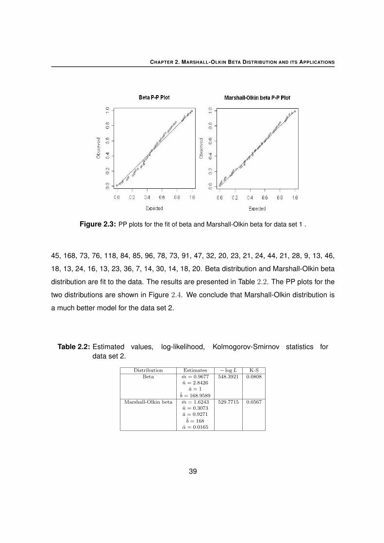
45, 168, 73, 76, 118, 84, 85, 96, 78, 73, 91, 47, 32, 20, 23, 21, 24, 44, 21, 28, 9, 13, 46,

18, 13, 24, 16, 13, 23, 36, 7, 14, 30, 14, 18, 20. Beta distribution and Marshall-Olkin beta

distribution are fit to the data. The results are presented in Table 2.2. The PP plots for the

two distributions are shown in Figure 2.4. We conclude that Marshall-Olkin distribution is

a much better model for the data set 2.

Table 2.2: Estimated values, log-likelihood, Kolmogorov-Smirnov statistics fordata set 2.

Distribution Estimates − log L K-SBeta m = 0.9677 548.3921 0.0808

n = 2.8426a = 1

b = 168.9589Marshall-Olkin beta m = 1.6243 529.7715 0.0567

n = 0.3073a = 0.9271

b = 168α = 0.0165

39


Figure 2.4: PP plots for the fit of beta and Marshall-Olkin beta for data set 2 .

2.8 Conclusions

We have developed a new beta distribution called Marshall-Olkin beta distribution and its

various properties are discussed. We have dealt with the estimation problem also. Some

data analysis is also done. Also we have developed a time series model with minification

structure and derived its autocovariance structure.

Appendix 1

Here we present a program which can be used to compute the moments of a randomvariable with MOBeta(m,n, 0, 1, α) distribution. The program is written in R.

hyper3f2<-function(u1,u2,u3,v1,v2) {

s0<-1

s1<-u1*u2*u3/(v1*v2)

sumHyper<-s0+s1

m1<-1

while (abs(s1-s0)>10^(-8)) {

s0<-s1

m1<-m1+1

s1<-s1*(u1+m1-1)*(u2+m1-1)*(u3+m1-1)/((v1+m1-1)*(v2+m1-1)*m1)

sumHyper<-sumHyper+s1

40


}

return(sumHyper)

}

sumVar<-function(ttt,l,v) {

if (l==1) {return(sum(v[1:(ttt+1)]*v[(ttt+1):1]))}

else {

sum1<-0

for (m1 in 0:ttt) {sum1<-sum1+v[m1+1]*sumVar(ttt-m1,l-1,v)}

return(sum1)

}

}

Kampe<-function(m,n,k,l,aa) {

a0<-1

v<-c(1,(1-n)*m/(m+1))

a1<-beta(n,aa+1)/beta(n,aa)*sumVar(1,l-1,v)

tt<-1

sumKampe<-a0+a1

while (abs(a1-a0)>10^(-8)) {

a0<-a1

tt<-tt+1

v[tt+1]<-v[tt]*(tt-n)*(m+tt-1)/((m+tt)*tt)

a1<-beta(n,aa+tt)/beta(n,aa)*sumVar(tt,l-1,v)

sumKampe<-sumKampe+a1

}

return(sumKampe)

}

moment<-function(m,n,p,k) {

if (p<1) {

sumVar<-beta(n,k+m)/beta(m,n)

aa0<-p*sumVar

sumVar[2]<-beta(n,k+2*m)/(m*beta(m,n)^2)*hyper3f2(k+2*m,1-n,m,n+k+2*m,m+1)

aa1<-2*p*(1-p)*(sumVar[1]-sumVar[2])

momentSum<-aa0+aa1

r<-2

while (abs(aa1-aa0)>=10^(-5)) {

r<-r+1

aa0<-aa1

sumVar[r]<-beta(n,k+r*m)/(m^(r-1)*beta(m,n)^r)*Kampe(m,n,k,r-1,k+m*r)

aa1<-r*p*(1-p)^(r-1)*sum(rep(c(1,-1),len=r)*choose(r-1,0:(r-1))*sumVar)

momentSum<-momentSum+aa1

print(c("r=",r,"momentSum=",momentSum))

}

return(momentSum)

41


}

else {

aa0<-1/p*beta(n,k+m)/beta(m,n)

aa1<-1/p*2*(1-1/p)*1/m*beta(n,k+2*m)/beta(m,n)^2*hyper3f2(k+2*m,1-n,m,n+k+2*m,m+1)

momentSum<-aa0+aa1

r<-2

while (abs(aa1-aa0)>=10^(-5)) {

r<-r+1

aa0<-aa1

aa1<-1/p*r*(1-1/p)^(r-1)*m^(1-r)*beta(n,k+r*m)/beta(m,n)^r*Kampe(m,n,k,r-1,k+m*r)

momentSum<-momentSum+aa1

print(c("r=",r,"momentSum=",momentSum))

}

return(momentSum)

}

}

Appendix 2

Program written in R for fitting the two beta distributions to the two datasets

# Marshall-Olkin beta DISTRIBUTION

# Probability density function of the Marshall-Olkin beta distribution

dMOBeta<-function(x,m,n,a,b,alpha) {

alpha*beta(m,n)*(x-a)^(m-1)*(b-x)^(n-1)/((b-a)^(m+n-1)*(alpha*beta(m,n)

+(1-alpha)*pbeta((x-a)/(b-a),m,n))^2)

}

# Distribution function of the Marshall-Olkin beta distribution

pMOBeta<-function(x,m,n,a,b,alpha) {

pbeta((x-a)/(b-a),m,n)/(alpha*beta(m,n)+(1-alpha)*pbeta((x-a)/(b-a),m,n))

}

FitMOBeta<-function(interval,p1,p2,p3,p4,p5) {

n<-length(y);

lInt<-length(interval);

estFreq<-real(lInt);

estFreq[1]<-round(n*pMOBeta(interval[1],p1,p2,p3,p4,p5),digits=4);

varSum<-estFreq[1];

for (i in 2:(lInt-1)) {

estFreq[i]<-round(n*(pMOBeta(interval[i],p1,p2,p3,p4,p5)-pMOBeta(interval[i-1],

p1,p2,p3,p4,p5)),digits=4)

varSum<-varSum+estFreq[i]

42


}

estFreq[lInt]<-n-varSum

estFreq

}

# Quantile function of the Marshall-Olkin beta distribution

qMOBeta<-function(p,m,n,a,b,alpha) {

z<-alpha*p/(1-(1-alpha)*p)

a+(b-a)*qbeta(z,m,n)

}

# Random generation of the Marshall-Olkin beta distribution

rMOBeta<-function(m,n,a,b,alpha,nobs) {

varSample<-real(nobs)

for (i in 1:nobs) {

z<-runif(1)

pom<-alpha*z/(1-(1-alpha)*z)

varSample[i]<-a+(b-a)*qbeta(pom,m,n)

}

varSample

}

# QQ plot for Marshall-Olkin beta distribution

qqMOBeta<-function(y,m,n,a,b,alpha) {

nn<-length(y);

x<-qMOBeta(ppoints(nn),m,n,a,b,alpha)[order(order(y))];

plot(y,x,main="Marshall-Olkin beta Q-Q Plot",xlab="Theoretical Quantile",ylab="Sample Quantiles");

z<-quantile(y,c(0.25,0.75));

xx<-qMOBeta(c(0.25,0.75),m,n,a,b,alpha);

slope<-diff(z)/diff(xx);

int<-z[1]-slope*xx[1];

abline(int,slope)

}

# PP plot for Marshall-Olkin beta distribution

ppMOBeta<-function(y,m,n,a,b,alpha) {

nn<-length(y);

yvar<-pMOBeta(sort(y),m,n,a,b,alpha);

xvar<-1:nn;

x<-(xvar-0.5)/nn;

plot(yvar,x,main="Marshall-Olkin beta P-P Plot",xlab="Expected",ylab="Observed");

curve(1*x,0,1,add=T)

}

####################################################################

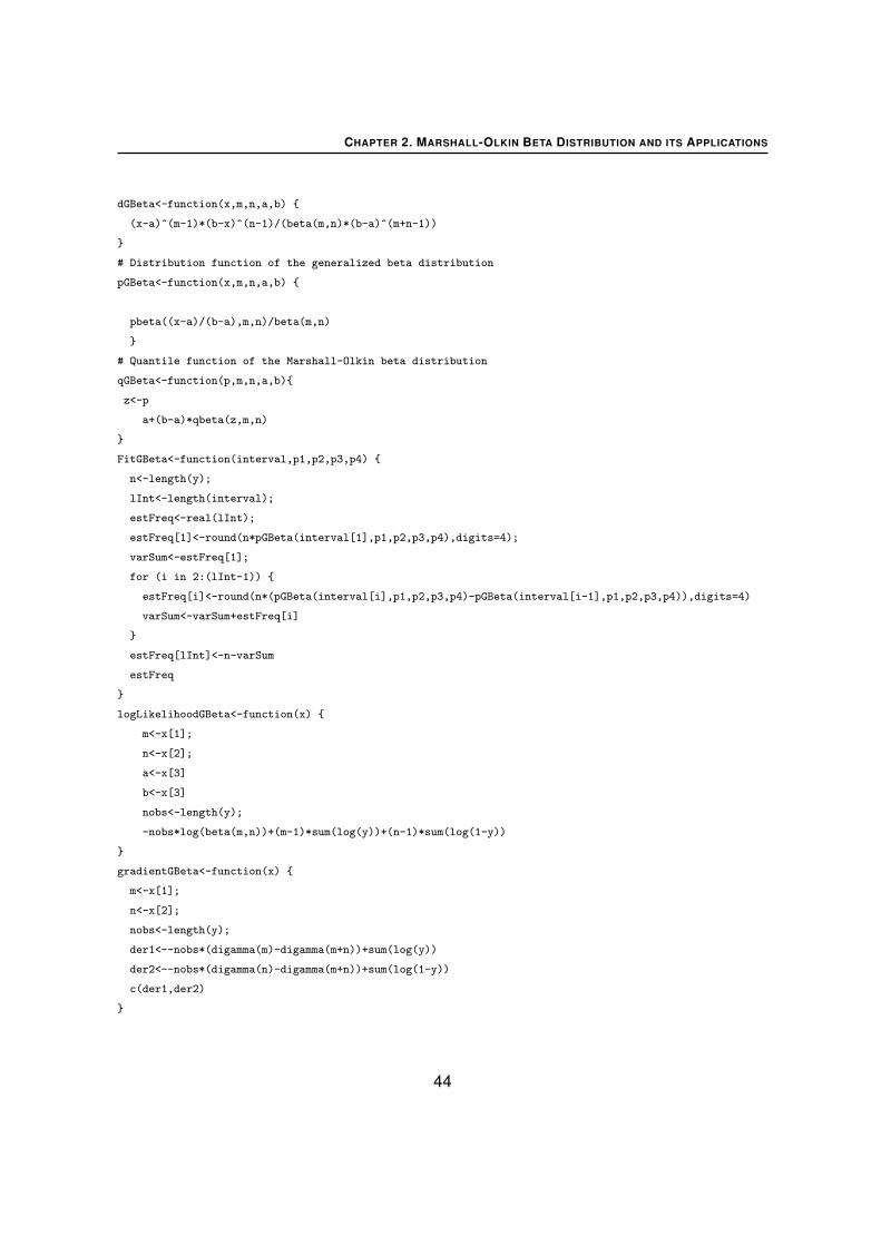
# Probability density function of the generalized beta distribution

43


dGBeta<-function(x,m,n,a,b) {

(x-a)^(m-1)*(b-x)^(n-1)/(beta(m,n)*(b-a)^(m+n-1))

}

# Distribution function of the generalized beta distribution

pGBeta<-function(x,m,n,a,b) {

pbeta((x-a)/(b-a),m,n)/beta(m,n)

}

# Quantile function of the Marshall-Olkin beta distribution

qGBeta<-function(p,m,n,a,b){

z<-p

a+(b-a)*qbeta(z,m,n)

}

FitGBeta<-function(interval,p1,p2,p3,p4) {

n<-length(y);

lInt<-length(interval);

estFreq<-real(lInt);

estFreq[1]<-round(n*pGBeta(interval[1],p1,p2,p3,p4),digits=4);

varSum<-estFreq[1];

for (i in 2:(lInt-1)) {

estFreq[i]<-round(n*(pGBeta(interval[i],p1,p2,p3,p4)-pGBeta(interval[i-1],p1,p2,p3,p4)),digits=4)

varSum<-varSum+estFreq[i]

}

estFreq[lInt]<-n-varSum

estFreq

}

logLikelihoodGBeta<-function(x) {

m<-x[1];

n<-x[2];

a<-x[3]

b<-x[3]

nobs<-length(y);

-nobs*log(beta(m,n))+(m-1)*sum(log(y))+(n-1)*sum(log(1-y))

}

gradientGBeta<-function(x) {

m<-x[1];

n<-x[2];

nobs<-length(y);

der1<--nobs*(digamma(m)-digamma(m+n))+sum(log(y))

der2<--nobs*(digamma(n)-digamma(m+n))+sum(log(1-y))

c(der1,der2)

}

44


functionGBeta<-function(x) {

res<--logLikelihoodGBeta(x);

attr(res,"gradient")<--gradientGBeta(x);

res

}

qqGBeta<-function(y,m,n,a,b) {

nn<-length(y);

x<-qGBeta(ppoints(nn),m,n,a,b)[order(order(y))];

plot(y,x,main="Beta Q-Q Plot",xlab="Theoretical Quantile",ylab="Sample Quantiles");

z<-quantile(y,c(0.25,0.75));

xx<-qGBeta(c(0.25,0.75),m,n,a,b);

slope<-diff(z)/diff(xx);

int<-z[1]-slope*xx[1];

abline(int,slope)

}

ppGBeta<-function(y,m,n,a,b) {

nn<-length(y);

yvar<-pGBeta(sort(y),m,n,a,b);

xvar<-1:nn;

x<-(xvar-0.5)/nn;

plot(yvar,x,main="Beta P-P Plot",xlab="Expected",ylab="Observed");

curve(1*x,0,1,add=T)

}

References

Alice, T., Jose, K.K. (2003). Marshall-Olkin Pareto Processes. Far East Journal of Theo-

retical Statistics, 9, 117-132.

Alice, T., Jose, K.K. (2004). Bivariate semi-Pareto Minification Processes. Metrika, 59,

305-313.

Alice, T., Jose, K.K. (2005a). Marshall-Olkin Semi-Weibull Minification Processes. Recent

Advances in Statistical Theory and Applications, I, 6-17.

Alice, T., Jose, K.K. (2005b). Marshall-Olkin logistic Processes. STARS Int. Journal, 6,

1-11.

45


Balakrishna, N., Jacob, T.M. (2003). Parameter estimation in minification processes,

Commun. Statist. Theory Methods, 32, 2139-2152.

Ed Mckenzie (1985). An autoregressive process for beta random variables, Management

Science, 31, 988-997.

Jayakumar, K., Thomas, M. (2007). On a generalization to Marshall-Olkin scheme and

its application to Burr type XII distribution. Statistical Papers,doi:10.1007/s00362-

006-0024-5.

Jose, K.K., Ancy, J. and Ristic, M.M. (2009). A Marshall-Olkin beta distribution and its

applications. Journal of Probability and Statistical Science,7(2),173-186.

Jose, K.K., Naik, S.R., Ristic, M.M. (2008). Marshall-Olkin q-Weibull distribution and

max-min Processes. Statistical Papers. doi:10.1007/s00362-008-0173-9.

Lewis, P.A.W., McKenzie, E. (1991). Minification processes and their transformations. J.

Appl. Prob. 28, 45-57.

Pillai, R.N. (1991). Semi-Pareto processes, J. Appl. Prob. 28, 461-465.

Marshall, A.W, Olkin, I. (1997). A new method of adding a parameter to a family of

distributions with application to the exponential and Weibull families. Biometrika,

84, 641-652.

McDonald, J.B., Xu, Y.J. (1995). A generalization of the beta distribution with applications.

J. Econometrics, 66, 133-152.

Nadarajah, S. (2007a). A truncated inverted beta distribution with application to air pollu-

tion data. Stoch. Environ. Res. Risk Assess, doi: 10.1007/s00477-007-0120-7.

Nadarajah, S. (2007b). Explicit expressions for moments of order statistics. Stat. Probab.

Lett., doi:10.1016/j.spl.2007.05.022.

46


Ricciardi, K.L., Pinder, G.F., Belitz, K. (2005). Comparison of the lognormal and beta

distribution functions to describe the uncertainty in permeability. J. Hydrology, 313,

248-256.

Sankaran, P.G., Jayakumar, K. (2007). On proportional odds models. Stat. Papers: doi:

10.1007/s00362-006-0042-3.

Sepanski, J.H., Kong, L. (2007). A family of generalized beta distributions for income.

arXiv.org,Stat.ME.

Sim, C.H. (1986). Simulation of Weibull and gamma autoregressive stationary processes,

Commun. Statist. Simulation Comput. 15, 1141–1146.

Sim, C.H. (1994). Modelling nonnormal first order autoregressive time series. J.Forecast.,

13, 369-381.

Yeh, H.C, Arnold B.C., Robertson, C.A. (1988). Pareto Processes, J. Appl. Prob., 25,

291-301.

Tavares, V.L. (1980). An exponential Markovian stationary process, J. Appl. Prob., 17,

1117-1120.

47

Documents

Marshall-Olkin Beta Distribution and its Applicationsshodhganga.inflibnet.ac.in/bitstream/10603/22815/10/10_chapter2.pdf · CHAPTER 2 Marshall-Olkin Beta Distribution and its Applications