Bivariate Beta Exponential Distributions - UGC …iosrjournals.org/iosr-jm/papers/Vol13-issue3/Version-1/B...Bivariate Beta Exponential Distributions DOI: 10.9790/5728-1303010719 9

IOSR Journal of Mathematics (IOSR-JM)

e-ISSN: 2278-5728, p-ISSN: 2319-765X. Volume 13, Issue 3 Ver. 1 (May. - June. 2017), PP 07-19

www.iosrjournals.org

DOI: 10.9790/5728-1303010719 www.iosrjournals.org 7 | Page

Bivariate Beta Exponential Distributions

Mervat K. Abd Elaal1,2

1 Statistics Department, Faculty of Sciences King Abdulaziz University Jeddah, Kingdom of Saudi Arabia

2 Statistics Department, Faculty of Commerce Al-Azhar University, Girls Branch Cairo, Egypt

Abstract: The exponential distribution is perhaps the most widely applied statistical distribution in reliability.

Anew continuous bivariate distribution called the bivariate beta-exponential distribution (BBE) that extends the

bivariate exponential distribution are proposed. We introduce a new bivariate beta-exponential distributions

(BBE) based on some types of copulas. Parametric and semiparametric methods are used to estimate the

parameters of the models. Finally, Simulation is studied to illustrate methods of inference discussed and

examine the satisfactory performance of the proposed distributions.

Key words: Beta exponential distribution, beta G distribution, bivariate beta exponential distributions;

Maximum likelihood method; copula;

I. Introduction The exponential distribution is a popular distribution the most widely used and applied for analyzing

lifetime data and for problems in reliability.

The exponential distribution is a popular distribution widely used for analyzing lifetime data. The

exponential distribution is perhaps the most widely applied statistical distribution for problems in reliability. In

this aim, we consider a generalization referred to as the beta exponential distribution generated from the logit of

a beta random variable. We work with the beta exponential (BE) distribution because of the wide applicability

of the exponential distribution and the fact that it extends some recent developed distributions. An application is

illustrated to a real data set with the hope that it will attract more applications in reliability, biology and other

areas of research.

Eugene et al. (2002) introduced the beta distribution as a generator to suggest the so-called family of

beta G distributions. The cumulative distribution function (c.d.f.) of a beta-G random variable X is defined as

F

(1)

for G(x) is the cdf of any random variable, a > 0 and b > 0, where = / denotes the

incomplete beta function ratio, and

denotes the incomplete beta function.

The p.d.f. corresponding to the beta-G distribution in (1) is given by

(2)

where g(x) = dG(x)/dx is the pdf of the parent distribution. The pdf f(x) will be most tractable when the

functions G(x) and g(x) have simple analytic expressions.

This family of distributions is a generalization of the distributions of order statistics for the random

variable X with cdf F(x) as pointed out by Eugene, et al. (2002) and Jones (2004). Since the paper by Eugene et

al. (2002), many beta-G distributions have been studied in the literature including the beta-Gumbel distribution

by Nadarajah and Kotz (2004), beta exponential distribution by Nadarajah and Kotz (2006), beta-Weibull

distribution by Famoye et al.(2005) and Cordeiro et al., (2011).

For more details, see, also, the beta-Pareto distribution by Akinsete, et al. (2008), beta modified

Weibull distribution by Silva et al.(2010), beta generalized half-normal distribution by Pescim et al., (2010),

And ,also, the beta Burr XII distribution by Paranaiba, et al., (2011), beta extended Weibull distribution by

Cordeiro, et al.(2012),beta exponentiated Weibull by Cordeiro et al.(2013),beta-lindley distribution by Merovci

and Sharma (2014), beta Burr type X distribution by Merovci et al.,(2016).

Eugene et al. (2002) introduced the beta normal distribution by taking G(x) in (1) to be the cdf of the

normal distribution. Nadarajah and Kotz (2004) introduced the beta Gumbel (BG) distribution by taking G(x) to

be the cdf of the Gumbel distribution. Also, Nadarajah and Kotz (2006) studied the BE distribution and obtained

the moment generating function, the asymptotic distribution of the extreme order statistics and discussed the

maximum likelihood estimation. For more details, see Azzalini(1985), Alexander, et al., (2012),Nadarajah and

Rocha (2016a), Nadarajah and Rocha (2016b), Alzaatreh et al., (2013), Aljarrah et al., (2014), Nadarajah, et al.,

(2015).

Beta exponential distribution used effectively in different lifetime applications. Nadarajah and Kotz

(2006) first introduced it.



We now study the BE distribution by taking G(x) in (1) to be the cdf of the exponential (E) distribution. Then,

the beta exponential (BE) distribution with three parameters α > 0, a > 0 and b >0 with the following Cdf and

the pdf, respectively,

The simple formula for the cdf of BE distribution if a, bare real integer given by

(3)

And, the pdf given by

(4)

And the hazard rate function given by

(5)

The moment generating function (mgf) of the BE distribution if b>2 is integer is given by

The simple formula for the mgf of BE distribution is given by

(6)

The r th moment of the BE distribution if b is integer can be obtain from

(7)

The first four moments of the BE distribution if b>0 is integer are obtain, respectively,

Where

𝜓 𝜓

𝜓 𝜓 𝜓

𝜓 𝜓 𝜓 𝜓

𝜓 𝜓

𝜓 𝜓 𝜓 𝜓 𝜓

𝜓 The BE distribution contains as special cases three well-known distributions. For example, it simplifies

to the BW distribution when. If α = 1, the BE distribution becomes the beta standard exponential (BSE)

distribution, If b = 1, the BE distribution becomes the EE distribution, The Exponential distribution is clearly a

special case for a = b = 1.

Copulas are a general tool to construct multivariate distributions and to find dependence structure

between random variables. However, the concept of copula is popular in multivariate analyses. In this aim, we

show that copulas can be important used to solve many statistical problems. Stated that any multivariate

distribution can be disintegrated to a copula and its continues marginal.

The Gaussian copula gives the following form

, (8)

where denotes the distribution function of a bivariate standard normal random variable and represents its

inverse.

The Farlie-Gumbel-Morgensten copula (FGM) takes the following form

(9)

where and , and is a dependence parameter.



Although the FGM copula family is tractable mathematically, it does not model high dependences. The range of

the dependence measures Kendall’s tau and Spearman’s rho ρ are and ρ respectively.

The Plackett copula takes the following form

, )1(2

)1(4)])(1(1[

)1(2

))(1(1v)C(u,

2

uvvuvu (10)

Where The correlation measure Spearman's rho is ρ

. There is no closed

expression in for the correlation measure Kendall's tau.

Several multivariate and bivariate lifetime distributions are derived using copula functions such as

Johnson, et al.(1992), Nelsen(1999),Adham and Walker, (2001),Trivedi and Zimmer, (2005),Adham, et al.

(2009), Kundu, et al.(2009), Kunduet al. (2010), Kundu and Gupta, (2011), Ateya and Al-Alazwari, (2013),

Sarabia et al. (2014), Abd Elaal et al.(2016), Adham et al. (2016), and Abd Elaal et al.(2017).

The main article of this article is to introduce bivariate beta exponential (BBE) models based on most

used copula functions in the literature as the Gaussian, Frank, Clayton, and Farlie-Gumbel-Morgensten (FGM)

and suggest which of them is more suitable. In addition, the performance of the proposed BBE will be examined

using a real data example.

The contents of this aim are as follows. Section 2 introduce three new bivariate beta exponential (BBE)

models based on different copula functions. Parametric and semiparametric methods are used to estimate the

parameters of BBE models in Section 3. In Section 4, goodness of fit test for the three models of bivariate beta

exponential (BBE) models computed to check the flexibility of different models based on different copula

functions. Finally, Simulation is studied to illustrate the performance of the suggested bivariate models and

compare each one to other bivariate models in Section 5.

II. Bivariate BE Distributions Based On Copulas For the bivariate case, copulas are used to link two marginal distributions with joint distribution such

that for every bivariate distribution function with continuous marginal , there exist a

unique copula function C as follows

(11)

The density function of bivariate distribution gives as

(12)

Where is the density function of copula.

see (Nelsen, 1999). Several copula functions can be used to construct BBE distributions with BE marginals

given by (4). In this article, we will applied the Gaussian, Farlie-Gumbel-Morgensten and Plackett copulas to

construct BBE distributions.

The joint PDF of and based on Gaussian copula becomes

where is a dependence parameter.

Figure (1): Plots the PDF and Cdf of the BBE based on Gaussian copula



Figure (2): Contour plots of BBEbased on Gaussian copula for different values of .

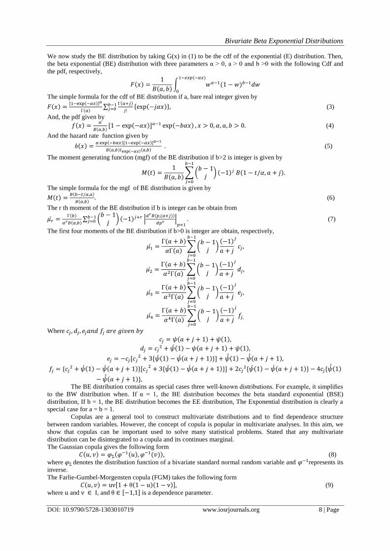
The joint PDF of and based on Farlie-Gumbel-Morgensten copula becomes

(14)


Figure (3): Plots the PDF and Cdf of the BBE based on FGM copula

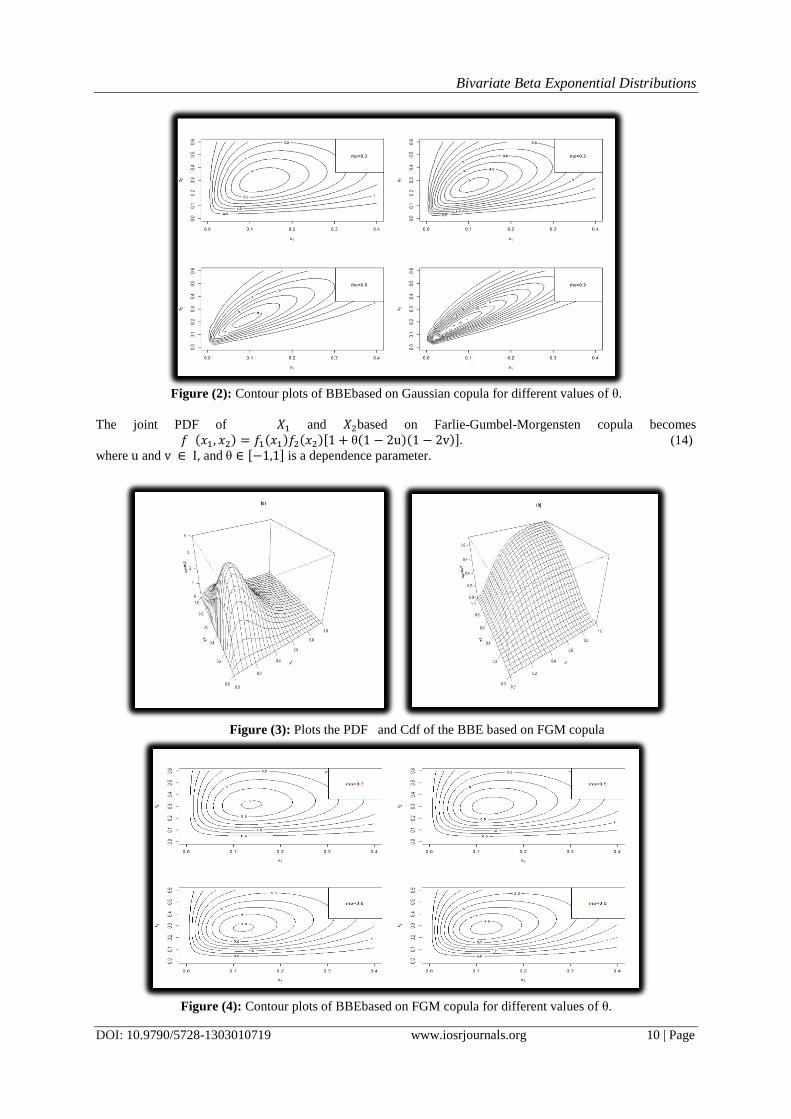
Figure (4): Contour plots of BBEbased on FGM copula for different values of .



The joint PDF of and based on Plackett copula becomes

(15)


Figure (5): Plots the PDF and Cdf of the BBE based on Plackett copula

Figure (6): Contour plots of BBEbased on Plackett copula for different values of .

III. Parameters Estimation In this section, we provide the estimation of the unknown parameters of BBE distributions by two

approaches to fitting copula models. Parametric and semiparametric are methods used to estimate proposed

distribution parameters.

3.1 Parametric methods of estimation:

There are two approaches to fitting copula models. The first one approach is two steps procedure

estimating the marginal and the copula parameter separately. The second approach is two steps procedure

estimating the marginal and the copula parameter, which is computed from the pseudo-observations separately.



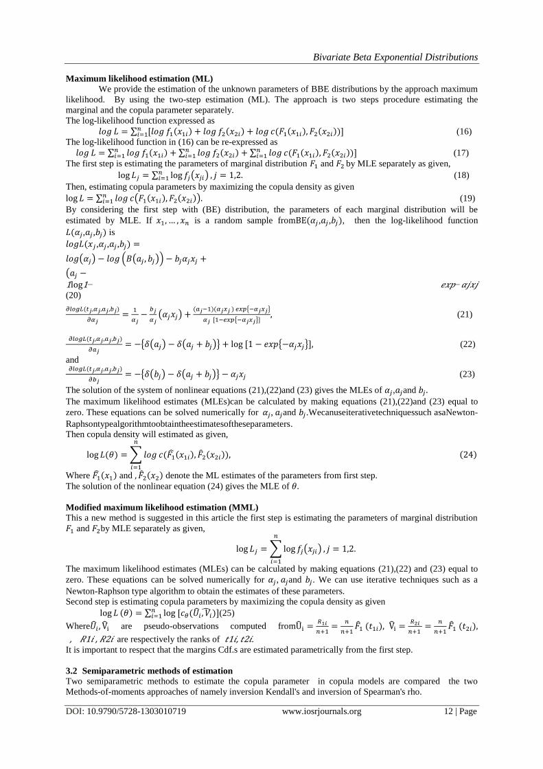
Maximum likelihood estimation (ML)

We provide the estimation of the unknown parameters of BBE distributions by the approach maximum

likelihood. By using the two-step estimation (ML). The approach is two steps procedure estimating the

marginal and the copula parameter separately.

The log-likelihood function expressed as

(16)

The log-likelihood function in (16) can be re-expressed as

(17)

The first step is estimating the parameters of marginal distribution and by MLE separately as given,

(18)

Then, estimating copula parameters by maximizing the copula density as given

(19)

By considering the first step with (BE) distribution, the parameters of each marginal distribution will be

estimated by MLE. If is a random sample from , , , then the log-likelihood function

, , is

, , ,

1log1− − (20)

(21)

(22)

and

(23)

The solution of the system of nonlinear equations (21),(22)and (23) gives the MLEs of , and

The maximum likelihood estimates (MLEs)can be calculated by making equations (21),(22)and (23) equal to

zero. These equations can be solved numerically for , and .Wecanuseiterativetechniquessuch asaNewton-

Raphsontypealgorithmtoobtaintheestimatesoftheseparameters.

Then copula density will estimated as given,

Where and denote the ML estimates of the parameters from first step.

The solution of the nonlinear equation (24) gives the MLE of

Modified maximum likelihood estimation (MML)

This a new method is suggested in this article the first step is estimating the parameters of marginal distribution

and by MLE separately as given,

The maximum likelihood estimates (MLEs) can be calculated by making equations (21),(22) and (23) equal to

zero. These equations can be solved numerically for , and . We can use iterative techniques such as a

Newton-Raphson type algorithm to obtain the estimates of these parameters.

Second step is estimating copula parameters by maximizing the copula density as given

(25)

Where are pseudo-observations computed from

, 1 , 2 are respectively the ranks of 1 , 2 . It is important to respect that the margins Cdf.s are estimated parametrically from the first step.

3.2 Semiparametric methods of estimation

Two semiparametric methods to estimate the copula parameter in copula models are compared the two

Methods-of-moments approaches of namely inversion Kendall's and inversion of Spearman's rho.



Methods-of-moments

Method-of-moments approaches of inversion Kendall's and inversion of Spearman's rho

As it is mentioned in Kojadinovic and Yan (2010) , let c be a bivariate random sample from

Cdf where F1 and F2 are continuous Cdf.s and is an absolutely continuous copula such

that , where is an open subset of . Furthermore, let are the vectors of ranks associated with

unless otherwise stated. In what follows, all vectors are row vectors. Method-of-moments approaches

are based on the inversion of a consistent estimator of a moment of the copula . The two best-known

moments, Spearman’s rho and Kendall’s tau, are respectively given by

ρ

, (26)

and

.

(27)

Consistent estimators of these two moments can be expressed as

(28)

And

(29)

When the functions ρ and are one-to-one, consistent estimators of are given by

,

It can be called inversion of Kendall's (itau) and inversion of Spearman's rho (irho) respectively. For more

information, see Kojadinovic and Yan (2010).

As explained above the methods-of-moments (itau) and (irho) estimation method for copula is considered as a

semiparametric method of estimation.

IV. Goodness Of Fit Tests For Copula

The idea of this test is to compare the empirical copula with the parametric estimator derived under the null

hypothesis see Dobrić and Schmid(2007) and Fermanian(2005). That is, test if C is well-represented by a

specific copula

Two approaches are commonly used in the literature to test the goodness of fit of a copula; the parametric

bootstrap see Genest and Rémillard (2008)or the fast multiplier approach see Genest, et al. ( 2009), and

Kojadinovicet al. ( 2011). The goodness of fit tests based on the empirical process

,

where is the empirical copula of the data of and

are pseudo observations from C calculated from data as follows

are respectively the ranks of

Here is a consistent estimator and is an estimator of obtained using the pseudo observations.

According to Genest et al.(2009), the test statistics is the Cramer-von Miss and is defined as

See for details Genest et al., (2009), Genest and Rémillard, (2008) and Kojadinovic et al., (2011).

V. Simulation Data In this section, a comparison between the three proposed models via different types of copulas is

presented. The correlation measures Kendall's tau and Spearman's rho of two variables with BBE distribution

are obtained and used to provide the values of copula parameters.

Considering the following values of marginal and copula parameters of BBE distribution based on Gaussian,

FGM and Plackett copulas with different sizes of sample (n = 20, 30, 50, 100,150 and 200):

α α Gaussiancopula parameter , FGM copula

parameter and Plackett copula parameter .



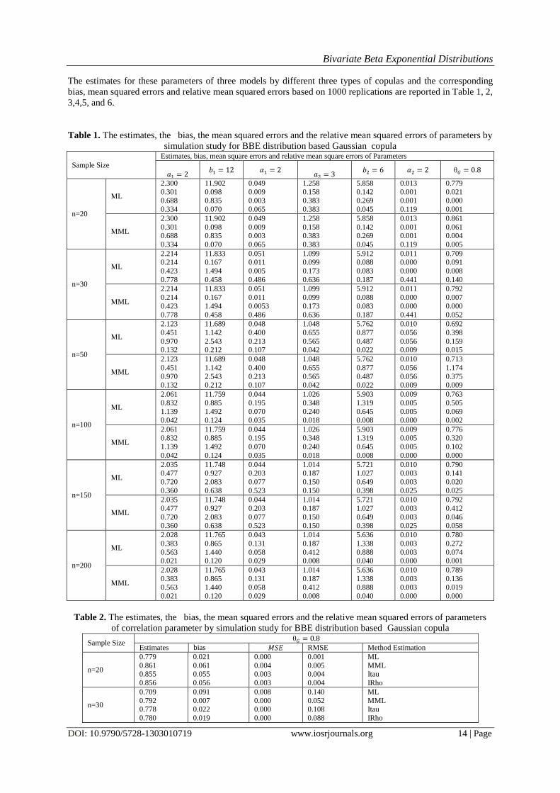
The estimates for these parameters of three models by different three types of copulas and the corresponding

bias, mean squared errors and relative mean squared errors based on 1000 replications are reported in Table 1, 2,

3,4,5, and 6.

Table 1. The estimates, the bias, the mean squared errors and the relative mean squared errors of parameters by

simulation study for BBE distribution based Gaussian copula

Sample Size

Estimates, bias, mean square errors and relative mean square errors of Parameters

n=20

ML

2.300

0.301 0.688

0.334

11.902

0.098 0.835

0.070

0.049

0.009 0.003

0.065

1.258

0.158 0.383

0.383

5.858

0.142 0.269

0.045

0.013

0.001 0.001

0.119

0.779

0.021 0.000

0.001

MML

2.300

0.301 0.688

0.334

11.902

0.098 0.835

0.070

0.049

0.009 0.003

0.065

1.258

0.158 0.383

0.383

5.858

0.142 0.269

0.045

0.013

0.001 0.001

0.119

0.861

0.061 0.004

0.005

n=30

ML

2.214 0.214

0.423

0.778

11.833 0.167

1.494

0.458

0.051 0.011

0.005

0.486

1.099 0.099

0.173

0.636

5.912 0.088

0.083

0.187

0.011 0.000

0.000

0.441

0.709 0.091

0.008

0.140

MML

2.214 0.214

0.423

0.778

11.833 0.167

1.494

0.458

0.051 0.011

0.0053

0.486

1.099 0.099

0.173

0.636

5.912 0.088

0.083

0.187

0.011 0.000

0.000

0.441

0.792 0.007

0.000

0.052

n=50

ML

2.123

0.451

0.970 0.132

11.689

1.142

2.543 0.212

0.048

0.400

0.213 0.107

1.048

0.655

0.565 0.042

5.762

0.877

0.487 0.022

0.010

0.056

0.056 0.009

0.692

0.398

0.159 0.015

MML

2.123

0.451

0.970 0.132

11.689

1.142

2.543 0.212

0.048

0.400

0.213 0.107

1.048

0.655

0.565 0.042

5.762

0.877

0.487 0.022

0.010

0.056

0.056 0.009

0.713

1.174

0.375 0.009

n=100

ML

2.061

0.832

1.139

0.042

11.759

0.885

1.492

0.124

0.044

0.195

0.070

0.035

1.026

0.348

0.240

0.018

5.903

1.319

0.645

0.008

0.009

0.005

0.005

0.000

0.763

0.505

0.069

0.002

MML

2.061 0.832

1.139

0.042

11.759 0.885

1.492

0.124

0.044 0.195

0.070

0.035

1.026 0.348

0.240

0.018

5.903 1.319

0.645

0.008

0.009 0.005

0.005

0.000

0.776 0.320

0.102

0.000

n=150

ML

2.035 0.477

0.720

0.360

11.748 0.927

2.083

0.638

0.044 0.203

0.077

0.523

1.014 0.187

0.150

0.150

5.721 1.027

0.649

0.398

0.010 0.003

0.003

0.025

0.790 0.141

0.020

0.025

MML

2.035

0.477

0.720 0.360

11.748

0.927

2.083 0.638

0.044

0.203

0.077 0.523

1.014

0.187

0.150 0.150

5.721

1.027

0.649 0.398

0.010

0.003

0.003 0.025

0.792

0.412

0.046 0.058

n=200

ML

2.028

0.383

0.563 0.021

11.765

0.865

1.440 0.120

0.043

0.131

0.058 0.029

1.014

0.187

0.412 0.008

5.636

1.338

0.888 0.040

0.010

0.003

0.003 0.000

0.780

0.272

0.074 0.001

MML

2.028

0.383 0.563

0.021

11.765

0.865 1.440

0.120

0.043

0.131 0.058

0.029

1.014

0.187 0.412

0.008

5.636

1.338 0.888

0.040

0.010

0.003 0.003

0.000

0.789

0.136 0.019

0.000

Table 2. The estimates, the bias, the mean squared errors and the relative mean squared errors of parameters

of correlation parameter by simulation study for BBE distribution based Gaussian copula

Sample Size

Estimates bias RMSE Method Estimation

n=20

0.779

0.861 0.855

0.856

0.021

0.061 0.055

0.056

0.000

0.004 0.003

0.003

0.001

0.005 0.004

0.004

ML

MML Itau

IRho

n=30

0.709

0.792 0.778

0.780

0.091

0.007 0.022

0.019

0.008

0.000 0.000

0.000

0.140

0.052 0.108

0.088

ML

MML Itau

IRho



n=50

0.692 0.713

0.680

0.668

0.398 1.174

0.442

0.487

0.159 0.375

0.195

0.327

0.015 0.009

0.018

0.022

ML MML

Itau

IRho

n=100

0.763

0.776

0.749 0.742

0.505

0.320

0.695 0.788

0.069

0.102

0.131 0.169

0.002

0.000

0.003 0.004

ML

MML

Itau IRho

n=150

0.790

0.792

0.782 0.780

0.141

0.412

0.249 0.273

0.020

0.046

0.062 0.074

0.025

0.058

0.062 0.093

ML

MML

Itau IRho

n=200

0.780

0.789 0.786

0.783

0.272

0.136 0.183

0.224

0.074

0.019 0.034

0.050

0.001

0.000 0.000

0.000

ML

MML Itau

IRho

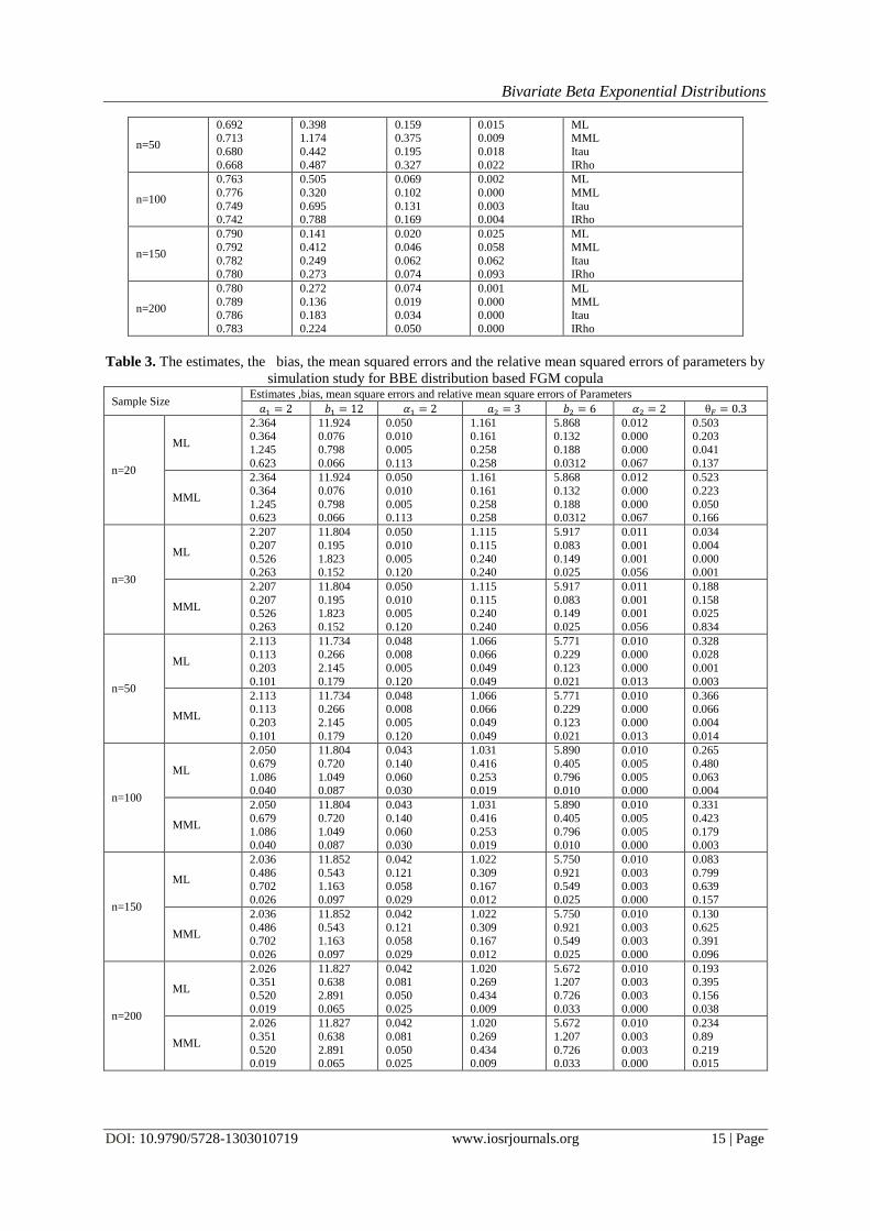
Table 3. The estimates, the bias, the mean squared errors and the relative mean squared errors of parameters by

simulation study for BBE distribution based FGM copula

Sample Size Estimates ,bias, mean square errors and relative mean square errors of Parameters

n=20

ML

2.364 0.364

1.245

0.623

11.924 0.076

0.798

0.066

0.050 0.010

0.005

0.113

1.161 0.161

0.258

0.258

5.868 0.132

0.188

0.0312

0.012 0.000

0.000

0.067

0.503 0.203

0.041

0.137

MML

2.364

0.364

1.245 0.623

11.924

0.076

0.798 0.066

0.050

0.010

0.005 0.113

1.161

0.161

0.258 0.258

5.868

0.132

0.188 0.0312

0.012

0.000

0.000 0.067

0.523

0.223

0.050 0.166

n=30

ML

2.207

0.207

0.526 0.263

11.804

0.195

1.823 0.152

0.050

0.010

0.005 0.120

1.115

0.115

0.240 0.240

5.917

0.083

0.149 0.025

0.011

0.001

0.001 0.056

0.034

0.004

0.000 0.001

MML

2.207

0.207 0.526

0.263

11.804

0.195 1.823

0.152

0.050

0.010 0.005

0.120

1.115

0.115 0.240

0.240

5.917

0.083 0.149

0.025

0.011

0.001 0.001

0.056

0.188

0.158 0.025

0.834

n=50

ML

2.113 0.113

0.203

0.101

11.734 0.266

2.145

0.179

0.048 0.008

0.005

0.120

1.066 0.066

0.049

0.049

5.771 0.229

0.123

0.021

0.010 0.000

0.000

0.013

0.328 0.028

0.001

0.003

MML

2.113 0.113

0.203

0.101

11.734 0.266

2.145

0.179

0.048 0.008

0.005

0.120

1.066 0.066

0.049

0.049

5.771 0.229

0.123

0.021

0.010 0.000

0.000

0.013

0.366 0.066

0.004

0.014

n=100

ML

2.050

0.679

1.086 0.040

11.804

0.720

1.049 0.087

0.043

0.140

0.060 0.030

1.031

0.416

0.253 0.019

5.890

0.405

0.796 0.010

0.010

0.005

0.005 0.000

0.265

0.480

0.063 0.004

MML

2.050

0.679

1.086 0.040

11.804

0.720

1.049 0.087

0.043

0.140

0.060 0.030

1.031

0.416

0.253 0.019

5.890

0.405

0.796 0.010

0.010

0.005

0.005 0.000

0.331

0.423

0.179 0.003

n=150

ML

2.036

0.486

0.702

0.026

11.852

0.543

1.163

0.097

0.042

0.121

0.058

0.029

1.022

0.309

0.167

0.012

5.750

0.921

0.549

0.025

0.010

0.003

0.003

0.000

0.083

0.799

0.639

0.157

MML

2.036

0.486 0.702

0.026

11.852

0.543 1.163

0.097

0.042

0.121 0.058

0.029

1.022

0.309 0.167

0.012

5.750

0.921 0.549

0.025

0.010

0.003 0.003

0.000

0.130

0.625 0.391

0.096

n=200

ML

2.026 0.351

0.520

0.019

11.827 0.638

2.891

0.065

0.042 0.081

0.050

0.025

1.020 0.269

0.434

0.009

5.672 1.207

0.726

0.033

0.010 0.003

0.003

0.000

0.193 0.395

0.156

0.038

MML

2.026

0.351

0.520 0.019

11.827

0.638

2.891 0.065

0.042

0.081

0.050 0.025

1.020

0.269

0.434 0.009

5.672

1.207

0.726 0.033

0.010

0.003

0.003 0.000

0.234

0.89

0.219 0.015



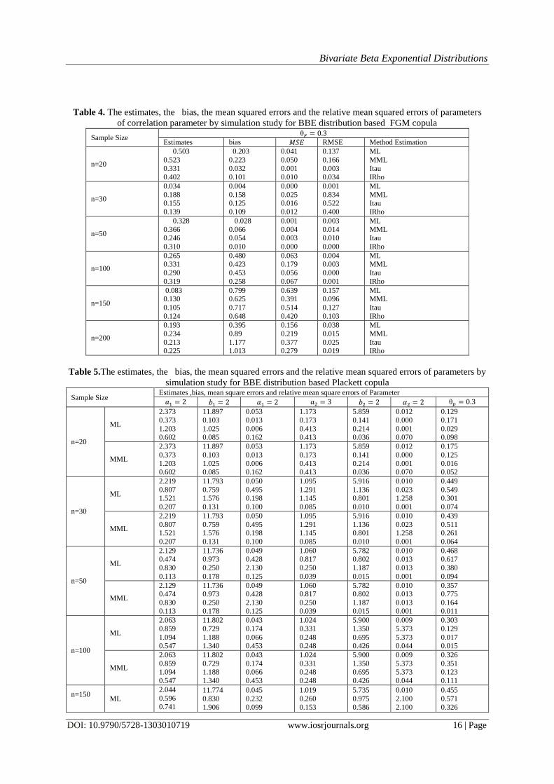
Table 4. The estimates, the bias, the mean squared errors and the relative mean squared errors of parameters

of correlation parameter by simulation study for BBE distribution based FGM copula

Sample Size


n=20

0.503

0.523

0.331 0.402

0.203

0.223

0.032 0.101

0.041

0.050

0.001 0.010

0.137

0.166

0.003 0.034

ML

MML

Itau IRho

n=30

0.034

0.188 0.155

0.139

0.004

0.158 0.125

0.109

0.000

0.025 0.016

0.012

0.001

0.834 0.522

0.400

ML

MML Itau

IRho

n=50

0.328

0.366 0.246

0.310

0.028

0.066 0.054

0.010

0.001

0.004 0.003

0.000

0.003

0.014 0.010

0.000

ML

MML Itau

IRho

n=100

0.265 0.331

0.290

0.319

0.480 0.423

0.453

0.258

0.063 0.179

0.056

0.067

0.004 0.003

0.000

0.001

ML MML

Itau

IRho

n=150

0.083 0.130

0.105

0.124

0.799 0.625

0.717

0.648

0.639 0.391

0.514

0.420

0.157 0.096

0.127

0.103

ML MML

Itau

IRho

n=200

0.193

0.234

0.213 0.225

0.395

0.89

1.177 1.013

0.156

0.219

0.377 0.279

0.038

0.015

0.025 0.019

ML

MML

Itau IRho

Table 5.The estimates, the bias, the mean squared errors and the relative mean squared errors of parameters by

simulation study for BBE distribution based Plackett copula

Sample Size Estimates ,bias, mean square errors and relative mean square errors of Parameter

n=20

ML

2.373

0.373

1.203 0.602

11.897

0.103

1.025 0.085

0.053

0.013

0.006 0.162

1.173

0.173

0.413 0.413

5.859

0.141

0.214 0.036

0.012

0.000

0.001 0.070

0.129

0.171

0.029 0.098

MML

2.373

0.373

1.203 0.602

11.897

0.103

1.025 0.085

0.053

0.013

0.006 0.162

1.173

0.173

0.413 0.413

5.859

0.141

0.214 0.036

0.012

0.000

0.001 0.070

0.175

0.125

0.016 0.052

n=30

ML

2.219

0.807 1.521

0.207

11.793

0.759 1.576

0.131

0.050

0.495 0.198

0.100

1.095

1.291 1.145

0.085

5.916

1.136 0.801

0.010

0.010

0.023 1.258

0.001

0.449

0.549 0.301

0.074

MML

2.219

0.807 1.521

0.207

11.793

0.759 1.576

0.131

0.050

0.495 0.198

0.100

1.095

1.291 1.145

0.085

5.916

1.136 0.801

0.010

0.010

0.023 1.258

0.001

0.439

0.511 0.261

0.064

n=50

ML

2.129 0.474

0.830

0.113

11.736 0.973

0.250

0.178

0.049 0.428

2.130

0.125

1.060 0.817

0.250

0.039

5.782 0.802

1.187

0.015

0.010 0.013

0.013

0.001

0.468 0.617

0.380

0.094

MML

2.129 0.474

0.830 0.113

11.736 0.973

0.250 0.178

0.049 0.428

2.130 0.125

1.060 0.817

0.250 0.039

5.782 0.802

1.187 0.015

0.010 0.013

0.013 0.001

0.357 0.775

0.164 0.011

n=100

ML

2.063

0.859

1.094 0.547

11.802

0.729

1.188 1.340

0.043

0.174

0.066 0.453

1.024

0.331

0.248 0.248

5.900

1.350

0.695 0.426

0.009

5.373

5.373 0.044

0.303

0.129

0.017 0.015

MML

2.063

0.859 1.094

0.547

11.802

0.729 1.188

1.340

0.043

0.174 0.066

0.453

1.024

0.331 0.248

0.248

5.900

1.350 0.695

0.426

0.009

5.373 5.373

0.044

0.326

0.351 0.123

0.111

n=150

ML

2.044

0.596 0.741

11.774

0.830 1.906

0.045

0.232 0.099

1.019

0.260 0.153

5.735

0.975 0.586

0.010

2.100 2.100

0.455

0.571 0.326



0.027 0.159 0.050 0.011 0.027 0.000 0.080

MML

2.044

0.596 0.741

0.027

11.774

0.830 1.906

0.159

0.045

0.232 0.099

0.050

1.019

0.260 0.153

0.011

5.735

0.975 0.586

0.027

0.010

2.100 2.100

0.000

0.406

0.389 0.151

0.037

n=200

ML

2.030

0.400 0.551

0.020

11.704

1.090 1.970

0.164

0.044

0.198 0.074

0.037

1.019

0.262 0.406

0.008

5.647

1.297 0.877

0.040

0.010

3.225 3.295

0.000

0.461

0.593 0.601

0.087

MML

2.030 0.400

0.551

0.020

11.704 1.090

1.970

0.164

0.044 0.198

0.074

0.037

1.019 0.262

0.406

0.008

5.647 1.297

0.877

0.040

0.010 3.225

3.295

0.000

0.456 0.573

0.329

0.081

Table 6. The estimates, the bias, the mean squared errors and the relative mean squared errors of correlation

parameter by simulation study for BBE distribution based Plackett copula

Sample Size


n=20

0.129

0.175

0.129 0.154

0.171

0.125

0.171 0.146

0.029

0.016

0.029 0.021

0.098

0.052

0.098 0.071

ML

MML

Itau IRho

n=30

0.449

0.439 0.403

0.419

0.549

0.511 0.380

0.438

0.301

0.261 0.145

0.199

0.074

0.064 0.036

0.047

ML

MML Itau

IRho

n=50

0.468

0.357 0.340

0.353

0.617

0.775 0.546

0.717

0.380

0.164 0.081

0.140

0.094

0.011 0. 005

0.009

ML

MML Itau

IRho

n=100

0.303 0.326

0.331

0.339

0.129 0.351

0.429

0.529

0.017 0.123

0.178

0.076

0.015 0.111

0.161

0.253

ML MML

Itau

IRho

n=150

0.455

0.406

0.425 0.434

0.571

0.389

0.462 0.495

0.326

0.151

0.213 0.245

0.037

0.080

0.052 0.060

ML

MML

Itau IRho

n=200

0.461

0.456

0.460 0.465

0.593

0.573

0.590 0.608

0.601

0.329

0.347 0.369

0.087

0.081

0.086 0.091

ML

MML

Itau IRho

From the results in Table 1,2, 3, 4, 5, and 6 we observed that

1. As expected, most results improve with increases in sample size.

2. For most selected values of , and the bias, MSE and RMSE of the estimates

, and become smaller as the sample size increases.

3. For greater than , the most results for are generally better than for Furthermore, the values of

get better more rapidly than the values of as the sample size increases.

4. For greater than , the most results for are generally better than for Furthermore, the values of

get better more rapidly than the values of as the sample size increases.

5. the efficient estimators of marginal parameters of three models differ according to the parameters. It seems

that ML estimates , and of three models are the same corresponding MML estimates.

6. For copula parameter, the MML provided efficient most estimates for Gaussian, FGM, and Plackett copula

parameters compared to ML, Itau, and Irho. It is also noted that the ML and MML estimates for all copula

parameters are close.

7. For copula parameter, it is observed that most estimates of Gaussian copula parameter were more

efficient than the corresponding the estimates of copula parameter and Plackett

copula .

To check if the selected parmetric copula functions are suitable for the marginals, goodness of fit test

statisticsusing selected copula functions for the marginals is preformed.The results in Table (7) show a non

signficant p-value obtained using parmetric bootstrap for all copula functions which indicate that selected



parmetric copula functions provide approporiate fit to the marginals. In addition, estimate of the copula parmeter

based on ML, MML, Itau, and Irho methods for the gussian, FGM, and Plackett copulas . This estimatesare used

as intial value when fitting these copula models using BE marginals.

Table 7. Goodness of fit test statistics with their p-values and estimate of the copula parameter for selected

copula functions. Copula Function

statistic p-value Estimate of copula parameter Method estimation

Gaussian

0.0139 0.6179 0.7986 Ml

0.0139 0.6578 0.7986 MML

0.0154 0.5679 0.7816 Itau

0.0157 0.5809 0.7799 Irho

FGM

0.0113 0.9915 0.1318 Ml

0.0113 0.9905 0.1318 MML

0.0119 0.9885 0.1051 Itau

0.0115 0.9915 0.1239 Irho

Plackett

0.0279 0.2003 0.4016 Ml

0.0279 0.1923 0.4016 MML

0.0241 0.2882 0.4255 Itau

0.0229 0.3601 0.4344 Irho

Acknowledgments

The author would like to thank the Editor-in-Chief, and the referee for constructive comments, which greatly

improved the paper.

References [1]. Abd Elaal, M. K. Adham, S. A., and Malaka, H. M. (2017). Goodness of fit tests for some copulas an application for gene data.

Advances and Applications in Statistical Sciences accepted. [2]. Abd Elaal, M. K., Mahmoud,M. R., El-Gohary, M.M., and Baharth,L.A. (2016). Univariate and bivariate Burr Type X

distributions based on mixtures and copula. International Journal of Mathematics and Statistics, 17(1),113-127.

[3]. Adham, S. A., Abd Elaal, M. K., and Malaka, H. M. (2016). Gaussian copula regression application. Journal International Mathematical Forum,11, 1053-1065.

[4]. Adham, S. A., and Walker, S. G. (2001). A multivariate Gompertz-type distribution. Journal of Applied Statistics, 28(8), 1051–

1065. [5]. Adham, S. A., AL-Dayian, G. R., El Beltagy, S. H., and Abd Elaal, M. K. (2009). Bivariate half- logistic-type distribution.

Academy of Business Journal, AL-Azhar University, 2, 92–107.

[6]. Alexander, C., Cordeiro, G.M., Ortega, E.M., and Sarabia, J.M. (2012). Generalized beta generated distributions.Computational Statistics and Data Analysis, 56, 1880–1897.

[7]. Akinsete A., Famoye F., Lee, C. (2008).The beta-Pareto distribution. Statistics 42(6), 547–563.

[8]. Aljarrah, M.A., Lee, C. and Famoye, F. (2014).On generating T-X family of distributions using quantile functions, Journal of Statistical Distributions and Applications 1, Article 2,

[9]. Alzaatreh, A., Lee, C., and Famoye, F. (2013). A new method for generating Families of continuous distributions. Metron, 71, 63–

79. doi:10.1007/s40300-013-0007-y. [10]. Ateya, S. F., and Al-Alazwari, A. A. (2013). A new multivariate generalized exponential distribution with application. Far East

Journal of Theoretical Statistics, 45(1), 51.

[11]. Azzalini, A. (1985). A class of distributions, which includes the normal ones. Scandinavian Journal of Statistics, 12, 171–178. [12]. Cordeiro, G.M., Gomes, A.E., da-Silva, C.Q., and Ortega, E.M. (2013). The beta exponentiated Weibull distribution. Journal of

statistical computation and simulation, 83(1),114–138.

[13]. Cordeiro, G.M., Silva, G.O. and Ortega, E.M.(2012).The beta extended Weibull distribution, Journal of Probability and Statistical Science (Taiwan), 10, 15–40.

[14]. Dobrić, J., and Schmid, F. (2007). A goodness of fit test for copulas based on Rosenblatt’s transformation. Computational Statistics

and Data Analysis, 51(9), 4633–4642. http://doi.org/10.1016/j.csda.2006.08.012 [15]. Eugene, N., Lee, C. and Famoye, F. (2002). Beta-normal distribution and its applications, Communications in Statistics–Theory and

Methods, 31, 497–512.

[16]. Famoye, f., lee, c. and olumolade, o. (2005). The beta-weibull distribution. Journal of Statistical Theory and Applications, 4, 121–136.

[17]. Fermanian, J.D. (2005). Goodness-of-fit tests for copulas. Journal of Multivariate Analysis, 95(1), 119–152.

http://doi.org/10.1016/j.jmva.2004.07.004 [18]. Genest, C., Ghoudi, K., and Rivest L. P., (1995). A semiparametric estimation procedure of dependence parameters in multivariate

families of distributions,Biometrika, 82( 3), 543–552. [19]. Genest, C., and Rémillard, B. (2008). Validity of the parametric bootstrap for goodness-of-fittesting in semiparametric models. In

Annales de l’IHP Probabilit{é}s et statistiques, 44, 1096–1127.

[20]. Genest, C., Rémillard, B., & Beaudoin, D. (2009). Goodness-of-fit tests for copulas: A review and a power study. Insurance: Mathematics and Economics, 44(2), 199–213.

[21]. Kojadinovic, I., and Yan, J. (2010). Comparison of three semiparametric methods for estimating dependence parameters in copula

models,Insurance: Mathematics and Economics,47( 1), 52–63. [22]. Kojadinovic, I., Yan, J., and Holmes, M. (2011). Fast large-sample goodness-of-fit tests for copulas. Statistica Sinica, 21(2), 841.

[23]. Jones,M. C. (2004). Families of distributions arising from distributions of order statistics (with discussion). Test, 13, 1–43.

[24]. Kundu, D., Balakrishnan, N., and Jamalizadeh, A. (2010). Bivariate Birnbaum--Saunders distribution and associated inference. Journal of Multivariate Analysis, 101(1), 113–125.

[25]. Kundu, D., and Gupta, R. D. (2009). Bivariate generalized exponential distribution. Journal of Multivariate Analysis, 100(4), 581–



593.

[26]. Kundu, D., and Gupta, R. D. (2011). Absolute continuous bivariate generalized exponential distribution. AStA Advances in

Statistical Analysis, 95(2), 169–185. [27]. Merovci, F., Khaleel, M.A., and Ibrahim, N.A.(2016). The beta Burr type X distribution properties with application. SpringerPlus,

5-697. DOI 10.1186/s40064-016-2271-9

[28]. Merovci, F., and Sharma, V.K.(2014).The beta-lindley distribution: properties and applications.Journal of Applied Mathematics,10-1989511–198951.

[29]. Nadarajah, S., Cordeiro, G.M. and Ortega, E.M.(2015).The Zografos-Balakrishnan–G family of distributions: Mathematical

properties and applications.Communications in Statistics– Theory and Methods, 44, 186–215. [30]. Nadarajah, S., and Kotz. S. (2004).The beta Gumbel distribution. Mathematical Problems in Engineering, 10, 323–332.

[31]. Nadarajah,S., and Kotz. S. (2006).The beta exponential distribution. Reliability Engineering and System Safety, 91, 689–697.

[32]. Nadarajah, S., and Rocha, R. (2016 a).Newdistns: An R Package for New Families of Distributions, Journal of Statistical Software, 69(10), 1-32, doi:10.18637/jss.v069.i10

[33]. Nadarajah, S., and Rocha, R. (2016 b). Newdistns: Computes PDF, CDF, Quantile and Random Numbers, Measures of Inference

for 19 General Families of Distributions. R package version 2.1, URL https://CRAN.R-project.org/package=Newdistns. [34]. Nelsen, R. B. (1999). An Introduction to Copulas. Springer&Verla, New York. Inc.

[35]. Paranaíba, P.F., Ortega, E.M., Cordeiro, G.M., and Pescim, R.R. (2011) The beta Burr XII distribution with application to lifetime

data. Computational Statistics and Data Analysis, 55(2),1118–1136. [36]. Pescim, R.R., Demétrio, C.G., Cordeiro, G.M., Ortega, E.M., and Urbano, M.R. (2010). The beta generalized half-normal

distribution. Computational Statistics and Data Analysis, 54, 945–957.

[37]. Sarabia,J.M., Prieto, F., and Jorda, V.,(2014). Bivariate beta-generated distributions with applications to well-being data. Journal of Statistical Distributions and Applications, 1-15.

[38]. Silva, G.O., Ortega, E. M.,and Cordeiro, G.M. (2010). The beta modified Weibull distribution. Lifetime Data Analysis, 16(3), 409–

430. [39]. Trivedi, P. K., and Zimmer, D. M. (2005). Copula modeling: an introduction for practitioners. Foundations and Trends in

Econometrics, 1(1), 1–111.

Documents

Bivariate Beta Exponential Distributions - UGC …iosrjournals.org/iosr-jm/papers/Vol13-issue3/Version-1/B...Bivariate Beta Exponential Distributions DOI: 10.9790/5728-1303010719 9