Embed Size (px)
Citation preview

7
Weak instruments and finite-sample bias
In this chapter, we consider the effect of weak instruments on instrumen-tal variable (IV) analyses. Weak instruments, which were introduced in Sec-tion 4.5.2, are those that do not explain a large proportion of the variation inthe exposure, and so the statistical association between the IV and the expo-sure is not strong. This is of particular relevance in Mendelian randomizationstudies since the associations of genetic variants with exposures of interest areoften weak. This chapter focuses on the impact of weak instruments on thebias and coverage of IV estimates.
7.1 Introduction
Although IV techniques can be used to give asymptotically unbiased estimatesof causal effects in the presence of confounding, these estimates suffer from biaswhen evaluated in finite samples [Nelson and Startz, 1990]. A weak instrument(or a weak IV) is still a valid IV, in that it satisfies the IV assumptions, and es-timates using the IV with an infinite sample size will be unbiased; but for anyfinite sample size, the average value of the IV estimator will be biased. Thisbias, known as weak instrument bias, is towards the observational confoundedestimate. Its magnitude depends on the strength of association between theIV and the exposure, which is measured by the F statistic in the regressionof the exposure on the IV [Bound et al., 1995]. In this chapter, we assumethe context of ‘one-sample’ Mendelian randomization, in which evidence onthe genetic variant, exposure, and outcome are taken on the same set of indi-viduals, rather than subsample (Section 8.5.2) or two-sample (Section 9.8.2)Mendelian randomization, in which genetic associations with the exposureand outcome are estimated in different sets of individuals (overlapping sets insubsample, non-overlapping sets in two-sample Mendelian randomization).
We illustrate this chapter using data from the CRP CHD Genetics Col-laboration (CCGC) to estimate the causal effect of blood concentrations of C-reactive protein (CRP) on plasma fibrinogen concentrations (Section 1.3). Asthe distribution of CRP is positively skewed, we take its logarithm and assumea linear relationship between log(CRP) and fibrinogen. Although log(CRP)
99
100 Mendelian Randomization
and fibrinogen are highly positively correlated (r = 0.45 to 0.55 in the ex-amples below), it is thought that long-term elevated levels of CRP are notcausally associated with an increase in fibrinogen.
We first demonstrate the direction and magnitude of weak instrument biasfor IV estimates from real and simulated data (Section 7.2). We explain whythis bias comes about, why it acts in the direction of the confounded observa-tional association, and why it is related to instrument strength (Section 7.3).We discuss simulated results that quantify the size of this bias for differentstrengths of instruments and different analysis methods (Section 7.4). Whenmultiple IVs are available, we show how the choice of IV affects the varianceand bias of IV estimators (Section 7.5). We propose ways of designing andanalysing Mendelian randomization studies to minimize bias (Section 7.6).We conclude with a discussion of this bias from both theoretical and practi-cal viewpoints, ending with a summary of recommendations aimed at appliedresearchers on how to design and analyse a Mendelian randomization studyto minimize bias from weak instruments (Section 7.7).
7.2 Demonstrating the bias of IV estimates
First, we demonstrate the existence and nature of weak instrument bias in IVestimation using both real and simulated data.
7.2.1 Bias of IV estimates in small studies
As a motivating example, we consider the Copenhagen General PopulationStudy [Zacho et al., 2008], a cohort study from the CCGC with completecross-sectional baseline data for 35 679 participants on CRP, fibrinogen, andthree SNPs from the CRP gene region: rs1205, rs1130864, and rs3093077. Wecalculate the observational estimate by regressing fibrinogen on log(CRP),and the IV estimate by the two-stage least squares (2SLS) method using allthree SNPs as IVs in a per allele additive model (Section 4.2.1). We thenanalyse the same data as if it came from multiple studies by dividing the datarandomly into substudies of equal size, calculating estimates of associationin each substudy, and combining the results using inverse-variance weightedfixed-effect meta-analysis. We divide the whole study into, in turn, 5, 10, 16,40, 100, and 250 substudies. We recall that the F statistic from the regres-sion of the exposure on the IV is used as a measure of instrument strength(Section 4.5.2).
We see from Table 7.1 that the observational estimate stays almost un-changed whether the data are analysed as one study or as several studies.However, as the number of substudies increases, the pooled IV estimate in-creases from near zero until it approaches the observational estimate. At the

Weak instruments and finite-sample bias 101
Substudies Observational estimate 2SLS IV estimate Mean F statistic
1 1.68 (0.01) -0.05 (0.15) 152.0
5 1.68 (0.01) -0.01 (0.15) 31.4
10 1.68 (0.01) 0.09 (0.14) 16.4
16 1.68 (0.01) 0.23 (0.14) 10.8
40 1.68 (0.01) 0.46 (0.13) 4.8
100 1.67 (0.01) 0.83 (0.11) 2.5
250 1.67 (0.01) 1.27 (0.08) 1.6
TABLE 7.1
Estimates of effect (standard error) of log(CRP) on fibrinogen (µmol/l) from
the Copenhagen General Population Study (N = 35 679) divided randomly
into substudies of equal size and combined using fixed-effect meta-analysis:
observational estimates using unadjusted linear regression, IV estimates using
2SLS. Mean F statistics averaged across substudies from linear regression of
log(CRP) on three genetic variants.
same time, the standard error of the pooled IV estimates decreases. We cansee that even where the number of substudies is 16 and the average F statisticis around 10, there is a serious bias. The causal estimate with 16 substudiesis positive (p = 0.09) despite the causal estimate with the data analysed asone study being near to zero.
7.2.2 Distribution of the ratio IV estimate
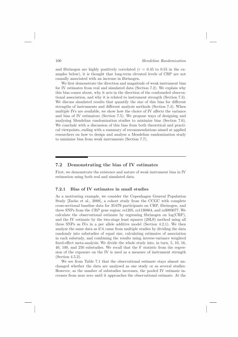
In order to investigate the distribution of IV estimates with weak instruments,we use a simulation exercise, taking a simple example of a confounded associa-tion with a single dichotomous IV [Burgess and Thompson, 2011]. Parametersare chosen such that the causal effect is null, but simply regressing the outcomeon the exposure yields a strong positive confounded observational associationof close to 0.5. We took 6 different values of the strength of the IV–exposureassociation, corresponding to mean F statistic values between 1.1 and 8.7.
Causal estimates are calculated using the ratio method, although with asingle IV the estimates from the ratio, 2SLS and limited information maxi-mum likelihood (LIML) methods are the same (Section 4.3.2). The resultingdistributions for the estimate of the causal parameter are shown in Figure 7.1.For weaker IVs, there is a marked bias in the median of the distribution inthe positive direction and the distribution of the IV estimate has long tails.For the weakest IV considered, the mean F statistic is barely above its nullexpectation of 1 and the median IV estimate is close to the confounded ob-servational estimate of 0.5. For stronger IVs, the median of the distributionof IV estimates is close to zero. The distribution is skew with more extremecausal estimates tending to take negative values.

102 Mendelian Randomization
The analyses in Table 7.1 and simulations in Figure 7.1 show that IVestimates can be biased. This bias has two notable features: it is larger whenthe F statistic for the IV–exposure relationship is smaller, and it is in thedirection of the confounded observational estimate.
7.3 Explaining the bias of IV estimates
We now try to provide some more intuitive understanding of why weak in-strument bias occurs. We give three separate explanations for its existence, interms of the definition of the ratio estimator, finite-sample violation of the IVassumptions, and sampling variation of IV estimators.
7.3.1 Correlation of IV associations
First, there is a correlation between the numerator (estimate of the G–Yassociation) and denominator (estimate of the G–X association) in the ratioestimator. To understand this, we consider a simple model of confoundedassociation with causal effect β1 of X on Y , with a dichotomous IV G =0 or 1, and further correlation between X and Y due to association with aconfounder U :
X = α1 G+ α2 U + εX (7.1)
Y = β1 X + β2 U + εY
U ∼ N (0, σ2
U ); εX ∼ N (0, σ2
X); εY ∼ N (0, σ2
Y ) independently.
We initially assume that σ2
X = σ2
Y = 0 for ease of explanation.If uj is the average confounder level for the subgroup with G = j (where
j = 0, 1), an expression for the causal effect from the ratio method is:
βR1 =
∆Y
∆X=
β1 ∆X + β2 ∆U
∆X= β1 +
β2 ∆U
α1 + α2 ∆U(7.2)
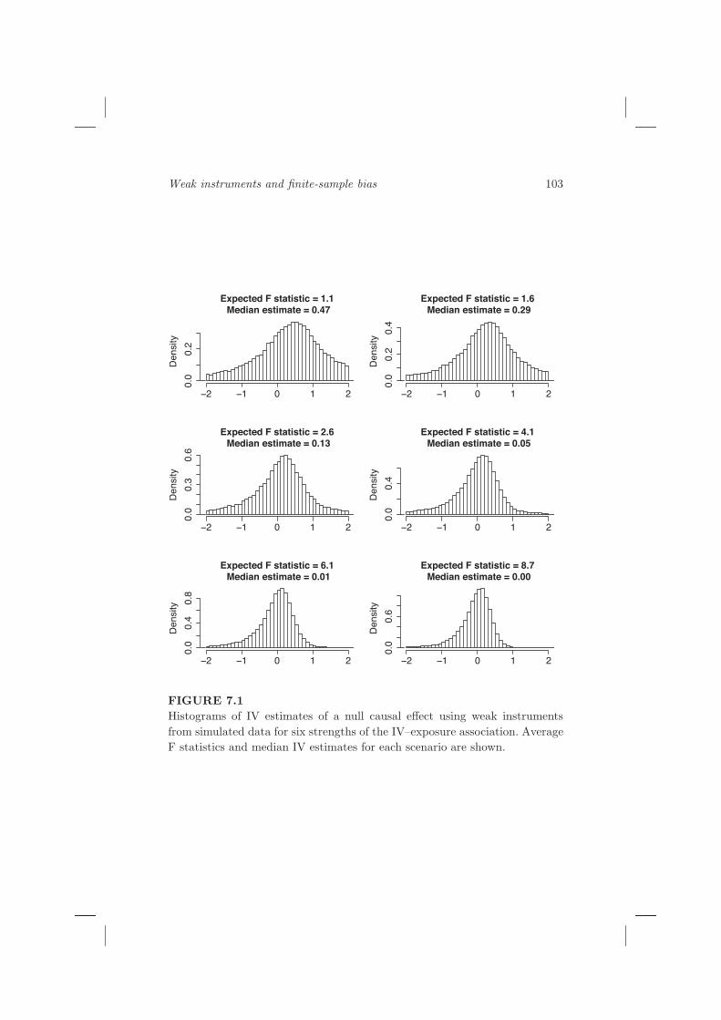
where ∆U = u1 − u0 is normally distributed with expectation zero; ∆X and∆Y are defined similarly. When the instrument is strong, α1 is large comparedto α2 ∆U . Then the expression βR
1will be close to β1. When the instrument is
weak, α1 may be small compared to β2 ∆U and α2 ∆U . Then the bias βR1 −β1
is close to β2
α2
, which is approximately the bias of the confounded observationalassociation (it is exactly this if α1 is zero). This is true whether ∆U is positiveor negative. Figure 7.2 (top panel) shows how the IV estimate bias varies with∆U . Although for any non-zero α1 the IV estimator will be an asymptoticallyconsistent estimator as sample size increases and ∆U tends towards zero, abias in the direction of the confounded association will be present in finitesamples. From Figure 7.2 (top panel), the median bias will be positive, as the
Weak instruments and finite-sample bias 103
Expected F statistic = 1.1 Median estimate = 0.47
De
nsity
−2 −1 0 1 2
0.0
0.2
Expected F statistic = 1.6 Median estimate = 0.29
Density
−2 −1 0 1 20.0
0.2
0.4
Expected F statistic = 2.6 Median estimate = 0.13
Density
−2 −1 0 1 2
0.0
0.3
0.6
Expected F statistic = 4.1 Median estimate = 0.05
Density
−2 −1 0 1 2
0.0
0.4
Expected F statistic = 6.1 Median estimate = 0.01
Density
−2 −1 0 1 2
0.0
0.4
0.8
Expected F statistic = 8.7 Median estimate = 0.00
Density
−2 −1 0 1 2
0.0
0.6
FIGURE 7.1
Histograms of IV estimates of a null causal effect using weak instruments
from simulated data for six strengths of the IV–exposure association. Average
F statistics and median IV estimates for each scenario are shown.

104 Mendelian Randomization
estimate is greater than β1 when ∆U > 0 or ∆U < −α1
α2
, which happens withprobability greater than 0.5.
This also explains the heavier negative tail in the histograms in Figure 7.1.The estimator takes extreme values when the denominator α1+α2 ∆U is closeto zero. Taking parameters α1, α2 and β2 as positive, as in the example of Sec-tion 7.2.2, this is associated with a negative value of ∆U , whence the numer-ator β2 ∆U will be negative. As ∆U has expectation zero, the denominatoris more likely to be small and positive than small and negative, giving morenegative extreme values of βR
1than positive ones.
If there is independent error in X and Y (that is, σ2
X and σ2
Y in equation(7.1) are non-zero), then the picture is similar, but more noisy, as seen inFigure 7.2 (bottom panel). The expression for the IV estimator is:
βR1 = β1 +
β2 ∆U +∆εY
α1 + α2 ∆U +∆εX
where ∆εX = εX1− εX0 and ∆εY = εY 1− εY 0 are defined analogously to ∆U
above.
7.3.2 Finite-sample violation of IV assumptions
An alternative explanation of weak instrument bias is in terms of violationof the second IV assumption in a finite sample. Although a valid instrumentwill be asymptotically independent of all confounders, in a finite sample therewill be a non-zero correlation between the instrument and confounders. Thiscorrelation biases the IV estimator towards the observational confounded as-sociation.
If the instrument is strong, then the difference in mean exposure betweengenetic subgroups will be mainly due to the genetic instrument, and the differ-ence in outcome (if any) will be due to this difference in exposure. However ifthe instrument is weak, that is it explains little variation in the exposure, thechance difference in confounders may explain more of the difference in meanexposure between genetic subgroups than the instrument. If the effect of theinstrument is near zero, then the estimate of the “causal effect” approachesthe association between exposure and outcome resulting from changes in theconfounders, which is the observational confounded association [Bound et al.,1995].
7.3.3 Sampling variation within genetic subgroups
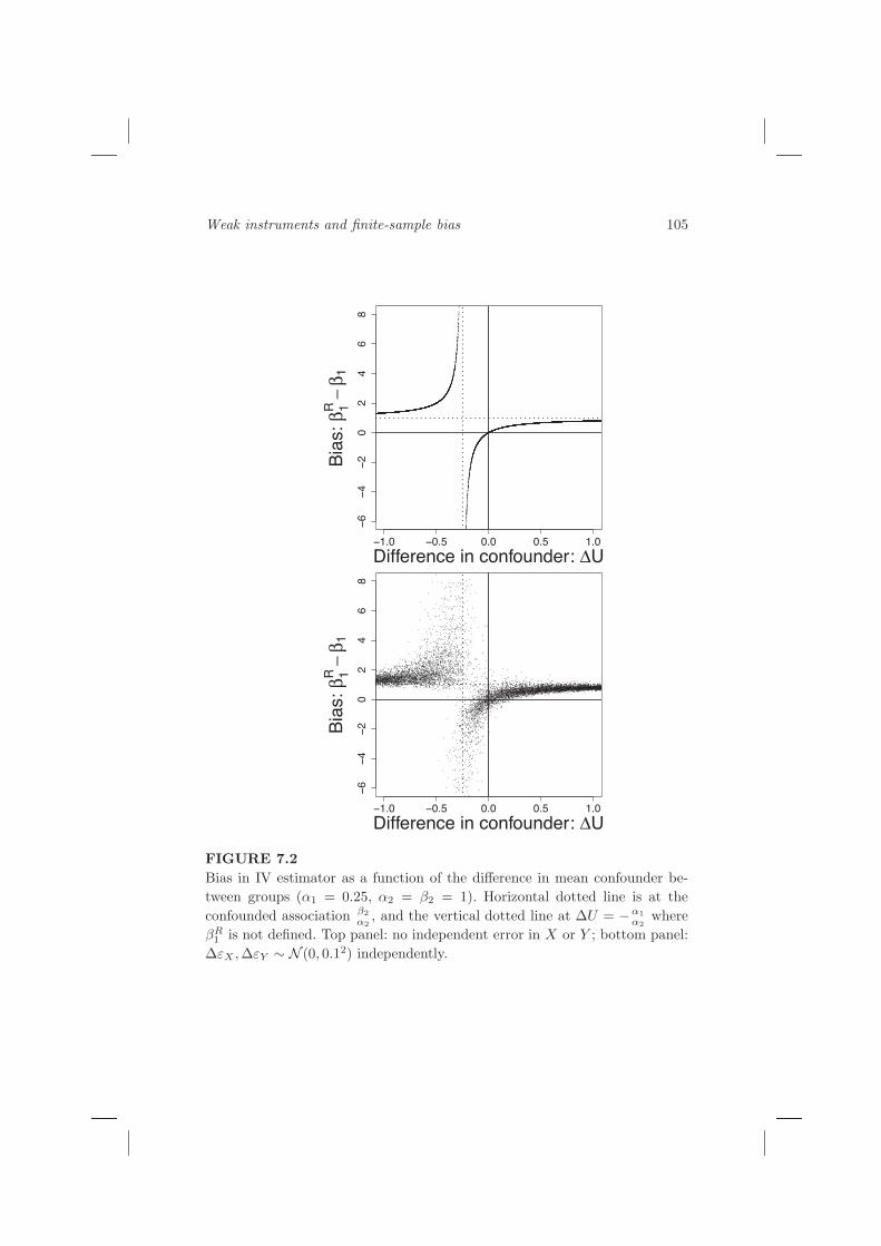
Finally, we offer a graphical explanation of weak instrument bias. To dothis, we simulate data with a negative causal effect of the exposure on theoutcome, but with positive confounding giving a strong positive observa-tional association between the exposure and outcome. We generate 1000 sim-ulated datasets with 600 subjects divided equally into three genetic subgroups
Weak instruments and finite-sample bias 105
−1.0 −0.5 0.0 0.5 1.0
−6
−4
−2
02
46
8
Difference in confounder: ∆U
Bia
s: β
1R−β
1
−1.0 −0.5 0.0 0.5 1.0
−6
−4
−2
02
46
8
Difference in confounder: ∆U
Bia
s: β
1R−β
1
FIGURE 7.2
Bias in IV estimator as a function of the difference in mean confounder be-
tween groups (α1 = 0.25, α2 = β2 = 1). Horizontal dotted line is at the
confounded association β2
α2
, and the vertical dotted line at ∆U = −α1
α2
where
βR1
is not defined. Top panel: no independent error in X or Y ; bottom panel:
∆εX ,∆εY ∼ N (0, 0.12) independently.

106 Mendelian Randomization
(G = 0, 1, or 2):
xi = α1gi + ui + εXi (7.3)
yi = β1xi + ui + εY i
ui ∼ N (0, σ2
U ); εXi ∼ N (0, σ2
X); εY i ∼ N (0, σ2
Y ) independently.
We set β1 = −0.4, σ2
U = 12, σ2
X = 0.22, and σ2
Y = 0.22, and take four val-ues for the strength of the IV (α1 = 0.5, 0.2, 0.1, and 0.05) correspondingto expected F statistics of 100, 16, 4.7, and 2.0. The mean levels of exposureand outcome for each genetic subgroup from each simulated dataset are plot-ted (Figure 7.3), representing joint density functions for each subgroup. Toexamine the sampling distribution of the IV estimate, we draw one point atrandom from each of these distributions; the gradient of the line through thesethree points is the 2SLS IV estimate. When the instrument is strong, the largedifferences in exposure between the subgroups due to variation in the IV willgenerally lead to estimating a negative effect of exposure on outcome. Whenthe instrument is weak, the differences in exposure between the subgroups dueto the IV are small and the positively confounded observational association ismore likely to be recovered.
7.4 Properties of IV estimates with weak instruments
In the previous section, we showed that IV estimates are biased in finite sam-ples. In this section, we consider the magnitude of the bias in IV estimates,as well as the coverage of IV methods with weak instruments.
7.4.1 Bias of IV estimates
The bias of an estimator is the difference between the expectation of theestimator and the true value of the parameter. In IV analysis, the relativemean bias is the ratio of the bias of the IV estimator (βIV ) to the bias of the
observational association (βOBS) found by linear regression of the outcome onthe exposure:
Relative mean bias =E(βIV )− β1
E(βOBS)− β1
. (7.4)
The relative mean bias from the 2SLS method is asymptotically approxi-mately equal to 1/E(F ), where E(F ) is the expected F statistic in the regres-sion of the exposure on the IV [Staiger and Stock, 1997]. This approximationis only valid when the number of IVs is at least three. The rule-of-thumb ofF < 10 indicating weak instruments (Section 4.5.2) derives from this expres-sion. This rule approximately limits the bias in the IV estimate to less than

Weak instruments and finite-sample bias 107
Strong instrument: E(F)=100
Exposure
Ou
tco
me
x
xxx
x
xx
xx
x
x
x x
xxx
xxx
x
x
xx
xx
x
xx
xx
x
x
x
xx
x
x
x
x
x
x
x
x
x
x
x
x
x
x
xx
x
xx
x
x
x
x
x
xxx
x
x
x
x
x
x x
x
x
x
x
x
x
x x
x
xxx
x
x
x
x
xx
x
xx
x
x
x
xxx
x
x
x
xx
xx
x
x
xx
xxx
xx
x
x
x
x
xxx
xx
x
xx x
xx
x
x
x
x
x
x
xx
x
xx
xx
x
xx
x
x
x
x xx
x
x
x
x
x
x xx
x
x
x xxxx
xx
x
xx
x
x
x
x
xx
x
xx
xxx
x
xx
xx
x xxxx
x
xx
xxx
x xx
x
x
xxx
x
x
x
x x
x
x
xx
xx
x
x
x
xx
x
x
xx
xx
xx
x
xx
x
xx
x
xxx
x
x
xx
x
xx
x
x
x
x
x
x
x
x
x
x x
xx
x
xx
xx
xxx
x
x
x
x
x x
x
x
x x
xx
x
x
xx
xx
x
xx
xx
x
xx
x
x
x
xx
x
x
x
xx
xx
x
xx
xx x
x
x
xx
x
x
xx
x
x
x
x
x
x
x
xxxx
x
x
x
xx
x
xx
x
x
x
x
xx
x
x
x
x
x
xx x
x
x
xx
x
x
x
xx
x
xx
x
x
x
x
x
x
x
x
xx
xx x
x
x
x
x
x
x
x
x
x
x
x
x
x
x
x
xx
x
x
x
x
x
x
xx
x
x xx
x
x
x
x
xx
x
x
x
x
x
x
x
x
x
x
x
x
xxx
x
xxx
x
x
x
x
x
x
xx
xx x
x
x
x
x
xx
x
x
x
x xxx
x
xx
xx
x
x
xx
x xx
x
x
xxxx
x
x
x
xx
xx
x
x
xx
x
xx
x
x x
x
xx
x
x
x
xxx
xx
x
x
xxx x
x
xx
x
x
x
xx
x
x
x
x
x
x
xx
x
x
x
x
xx
xxx
xx
x
x
x
x
xx
xx
x
x
x
xx
x
x
x
x
x
x
xx
x
x
x
x
x
x
x
x
x
xx
x
x
x
x
x
x
x
xx x
xxx
xx
x
x
xx xx
xx
x
x
x
x
x
x
x x
x
xx
x
xx
x
x
xxx
xx
x
x
x
x
x
x
xx
x
x
xxx x x
x
x
xx
x
x
x
xx
x x
x
x
xxx
x xx
xx
x
x
xx
xx
x
xx
x
x
xx
x
x
x
x
x
x
x x
xx
x
x
x
x
x
x
x x
x
xxx x
x
xxx
x
x
xx
xx
xxx
x
xx
x
x
xx
x
x
x
x
x
x
xxx
xxx
x
x
xx
x xxx
x
xx
x
x
x
x
x
x
x
x
xx
xx
x
xx
x
xxx
x
x
x
x
x
xxxxx
x
x
xx
x x
xx
x xx
x
x
x
x
x
x
x
xx x
x
xx
x
x
xx
x
x
x
x
x
xx
x
xx
xx
xx
x
x
xx
x
x
x
xxx
x
xxx
x
xxx
x
x
x
xx
x x
x
x
x
xx
xx
x
x
x
xx
x
x
xx
x
xx
xxxx
xxx
xx
xx
x
xxx x
x x
x
x
x
xx
xxx
x
x
x
xx
xx
x
x
xxx
xxxx
xx
x
xx
x
x
x
x
x
x
x
x
x
x
x
x
x
x
x
xxxx
x x
x x
x
x x
x
xx
xx xx
x
xx
x
xx
xx
xx
x
x
xx x
xx
x
xx
x
xx
x
xxx
xx
xx x
x
x
x
x
x
x
xx
x
xx
x
xx
x
x
x
x
xxx
xx
x
x
xx
x
x
x
x
x
x
x
x
x
xx
x
x
x
x
x
xx
x
x
x
o
o
o
o
o
o
oo
o
o
o
o
oo
o
o
oo
o
o
o
o
o
o o
o
oo
oo o
oo
o
o
o
o
oooo
o
ooo
o
ooo
o
o
o
o
o
o
o
o
o
o
o o oo
o
oo
o
o
oo
o
o
ooo o
ooo
o
oo
o
o
o
o
o
o
oo
oo
o
oo
o
oo
o
o
ooo
o
o
o
o
oo
o
o
o
oo
o
o
oo
o
o
o
o
o
o
o
o
o
oo
oo
oo
oo o
o
o
o
o
o
o
o
o
oo
oo
o
o
oo
o
o
oo
oo
o o
oo
o
o
o
o
o
o
oo
o
oo
o
oo
o
o
o
o
o
oo
oo
o
oo
oo
ooo o
o
o
oo
oo
o
o
ooo
o
o
o
o
o
ooo
o
o
o
o
o
o
o
o
oo
o
o
o
o
o
o
o
o
oo o
o
o
oo
o o
oo
oo
o
oo
oo
o
o
o
o
o
o
o
oo
oo
oo
o
oo
oo
ooo
o
o
o
o
o
o
oo
o
o
o
o
o
o
o
o
o
ooo
o
o
o
ooo
oo
o
o
o
oo
o
oo
oo
ooo
oo
o
o
o
oo
o
o
o
o
o
o
o
o oo o
o
oo
ooo
o
oo
o
ooo
oo
o
o
o
oooo o
ooo
o
o
o
o
o
oooo
o
o
o
o
oo
o
oo
ooo
o
o
o
o
o
o
oo
o
o
oo
o
o
oo
o
o
o
o
o
oo
o
o
o
oo
o
oo
o
ooo
o
o
oo
ooo
o
o
o
ooo
o
o
ooo oo
o
o
o
o
o
oo
o
o
o
o
o
o
o
o
o
o
o
oo
o
o
o
o
o
o
oo
o
oo
o
o
o
o
o
o
o
o
o
o
o
o
ooo
o
o
o
o
o
oo
o
oo
o
ooo
o
oo o
o
oo
o
o
o
o o
o
oo
o
oo
o
ooo
oo
oo
o
o
o
oo
o
oo
o
o
o
o
o
o
o
ooo
oooo
o
oo
oo
o
o
o
o
o
o
o
oo
o
oo
o
o
o
o
o
o
ooo
o
o
ooo
o
o
o
o
oo
o
o
o
o
o
oo
o
o
o
ooo
o
o
o
ooo
o o
oo
oo
o
oo
o
o
o
o
oooo
ooo
o
o
oo
o
oo
o
oo
o
ooo
o
oo
o
o
o
o
o
o
o
o
o
o
o
o
o
o
oo oo
o
o
o
o
o
o
o
o
o
o
o
o
o
o
o
ooo
o o oo
o
oo
o
o
o
o
ooo
o
oo
o
o
o
oo
o
oo
o
oo
oo
oo
o
o
oo
oo
o
o
o
o
o
oooo
oo
o
o
oo
o
o
ooo
o
o
o
oo
o
oo
o
o
o
o
o
o
o
o
o
ooo
o
o
o
o
oo oo
oo oo
o
o
o
oo
oo
o
o
o
o
o
o
o
o
o
o
oo
o
oo
o
oo
o
o
o
o
o
o
ooo
o
o
o
o
o
oo
o o
o
oo
o
o
o
o
o
o
o
o
o
oo
o
oo
o
o oo o
o
o
o
o
o
oo
ooo
o
o
o oo
o
o
o
o
o
oo
o
o
o
o
ooo
o o
o
o
o
o ooo
oo
o
o
o
o
o
o
o
o
o
oo
o
o
o
o
o
o
o
o
oo
o
ooo
o
o
o
o
o
oo
oo
ooo
o o
o
o
oo
oo
o
oo
oo
oo o
oo
o o
o
o
o
oo
oo
o
oo
o
o
oo
o
o
o
oo
o
o
o
o
o
o
o
oo
o
o
o
o
oo
o
oo
oo
o
o
o
o
oo
o
o
o
oo
o
o
o o
o
o
oo
o
oo
o
o
o
oo
ooo
o
o
o
o
o
oo
o
o
o
o
Moderate instrument: E(F)=16
Exposure
Ou
tco
me
x x
x
x
xx
x
x
x
x x
x
x
xxx
x
xx
x
x
x
x
x
x
x
xx
x
x
x
x
x
x
x
xx
x
x
x
x
x x
xx
x
xx
x
x
x
x
x
xx
xx
x
x
x
x
x
x
x
x
x
x
x
x
x
x
x
x
x
x
x
x
x
x
x
x
x
x
x
xx
x
x
x x
x
x
xx
x
x
xx
x
x
x
x
x
xx
x
x
x x
x
x
xx
xxxxx
x
x
x
x
x
x
x
x
x
x
x
x
x
x
x
x
x
x
x
x
x
x
xx
x
x
x x
x
x
x
x
x
x x
x
x
x
xx
x
x
x
x
x
x
x
xxx
x
x
x
xx
x
x
xx
x
xx
x
x
x
x
x
x
x
x
x
x
x
xx
xx
x
xx
xx
x
x
xx
x x
x
x
x
xx
x
x
x
x
x
x
x
xx
xx
x
x
x
x
x
x
xxx
x
x
x
x
x
x
x
x
x
x xx
x
xx
x
x
x x
xxx
x
x
x
x
x
xx
x
x
x
x
xx
x
x
x
x
x
x
x
x
x
x
x
x
x
x
xx
x
x
x
x
x
x
x
x
xx
x
xx
x x
x
xxx
x
x
x
x
x xx
x
x
x
xxx
xx
xx
x
x
x
x
x
x
x
xx
x x
x
x
x
x
x
x
x
x
xx
xx
x
xx
x x
x
xx
x
x
x
xx
x
x
x
x
x
x
x
x
x
x
x
xx
x
x
x
x
x
x
x
xx
x
x
x
x
xx x
x
x
x
x
x
x
xx
x
x
xxx
x
x
x
x
x
x
x
x
x
x
x
x
x
x
x
xx
x
x
x
x
x
x
x
x
x
xx
x
x
x
x
x
x
x
x
x
x
x
xx
x
x
xx
x
x
x
x
x
x
xx
x
x
x
x
x
xx
x
x
xx
x
x
x
x
xx
x
x
x x
x
x
x xx
x
x
x
x
x
x
x
x
x
x
x x
x
x
x
x
x
xx
xx
x
xxxx
x
x
xx
x
x
x
x
x
x
x
xx
x
x
xx
xx
x
x
xx
x
x
x
x
xx
x
x
x
x
x
x
x
x
x
x
x
xxx x
x
x
x
x
x
x
x x
x
x
xx
xx
x
x
x
x
x
x
xxx
xx
xx
x
x
xx
x
x
xxx
x
x
x
x
x
x
x
x x
x
xx
x
x
x
x
x
x
x
x
x
x
x
xx
x
x
x
x
x xxx
x
x
xx x
x
x
x
x
x
x
x
x
x
x
x
x
x
xx
x x
x
x
x
x
x
x
x
x
x
x
x
xx
x
x
x
x
xx
x
xx
x
x
x
x
x
xxx
x
x
x
x
x
x
x
x
x
x
x
x
x
x
x
x
x
x
x
x
x
xx
x
x
x
x
x
x
x
x
xx
xx
x
x
x
x
x
x
x
x
x
x xx
x
x x
x
x
x
x
x x
x
x
x
x
x
xx
x
x
x
x x
x
x
x
x
xx
xx
x
x
x
xxx
x
x
x
xx
x
x
x
x
x
xx
xx
x
x
xxx
x
x x
x
x
x
x
x
xxx
xx
x
x
x
x
x
xx
x
x
x
x
xx
x
x
x
x
x
x
x
x
x
x
x
x
x
xxx
xx
x
x
x
x
x
x
x
x
x
x
x
x
x
xx
x
x
x
x
xx
x
x
x
x
x
x
x
x
x
xx
x
x
x
x
x
x
x
x
x
x
x
x
x
x
x
xx
x
x
x
xx
x
xx
x
x
x
x
x
x
x
xx
xx
x
x
x
xx
x
x
x
x
xx
x
xx
x
x
x
xxx
x
x
x
x
x
x
x
x
x
x
xx
x
xx
x
xxx
x
x
x
x
x
x
xx x
xxx
x
x
xx
xx
x
x
xx
xx
x
x
x
x
x
x
x
x
xx
x
x
x
x
x
x
xx
x
x
x
xx
x
xx
x
x
xx
x
x
xx
x
x
x
x x
xxx
x xxx
x
x
xxx
x
x
x
x
x
xx
o o
o
oo
oo
o
o
o
o
o
o
o
oo
o
oo
oo o
oo
o
o
o
o
o
o
o
ooo
oo
oo
o
o
o
o
o
o
oo
o o
o
oo
o
oo
o
oo
o
o
oo
o
oo
oo
o
o
o
o
o
o
o
oo
o
o
o o
o
o
o
o
o
o
o
o
o
o
o
o
o
o
oo
o
o
o
oo
o
o
o
o
oo
o
o
o
o
o
oo
o
oo
oo
o
oo
oo
o
o o
o
ooo
o
o
o
o
o
o
o
o
o
o
o
oo
o
o
o
o
o
o
o
o
o
o
o
o
o
o
o
o
o
o
oo
o
o
o
o
o
o
o
o
oo
o
o
o
oo
o
o
o
o
o
o
o
o
oo
o
o
oo
o
o
o
o
o
o
o
o
o
o
o
o
o
o o
oo
o
o
o
o
o
o
o o
o
o
o
o
o
o
o
oo
o
o
ooo
oo
oo
oo
o
oo
o
oo
o
o
o
o
o
o
o
o
oo
o
o
o
o
o
o
o
oo
o
o
o
ooo
o
o oo
o
o
oo o
o
oo o
o
oo
o
o
o
o
o
o
o
oo
o
o
o
o
oo
o
o
o
o
oo
o
o
o
o
o
o
o o
o
oo
o
o
o
o
o
o
oo
o
o
o o
ooo
o
ooo o
oo
oo
oo
o
o
o
o
oo
oo
o
o
o
o
o
o
o
o
o
oo
o
o
o
o
o
o
o
oo
oo
o
o
oo
oo
o
o
o
oo
o
o
o
o
oo
o
o
o
o
o
o
o
oo
o o
o
o
o
oo
oo
o
o
o
o
o
o
o
o
o
o
o
o
o
o
oo
oo
oo
o
o
o
o
o
o
o
o
o
o
o
oo
o
o
o
o
o
o
o
o
o
o
o
o
o
o o
oo
o
o
o
o
o
o
o
o
o
o
o
o
oo
o
o
o
o
o
oo
o
o
o
o
o
o
o
o
o
o
ooo o
o
o
o
oo
o
oo
o
o
o
o
oo
o
o
o
o
o
oo
oo
o
o
o
o
o
o
ooo
o
o
oo
o
o
o
o
oo o
oo
o
o
oo
o
oo
o
o
o
o
o
o
o
o
o
o
o
o
o
o
o
o
o
oo
o
o
ooo
oo
o
o
o
o
oo
o
ooo
oo
o
oo
o
o
o
o o
o
o
o
o
oo
o
o
o
o
o
ooo
o
o
o
o
o
o
o
o
oo
o
o
o
o
oo
o
o
ooo
o
o
o
oo
o
o
o
o
o
o o
o
o
oo
o
o o
o
o
o
o
o
o
o
oo
o
o
oo
o
o
oo
o
o
o
o
o
o
o
o
o
o
o
o
o
o
o
o
o
o
o
o
o
o
o
o
o
o
o
o
o o
o
o
o
o
o
o
o
o
o
o
o
oo
o
o
o
o
o
o
o oo
o
o
o
o
o
o
o
o
oo
o
o
o
o
o
o
o
o
o
o
o
o
o
o
oo o
o
o
o
o
ooo
o
o
oo
o
oo
oo
o
o
o
o
o
o
o
oo
o
o
o
o
o
o
o
o
o
o
o
o
o
o
o
o
o
o
o
o
o
o
o
o
o
o
oo
o
oo
o
o o
o
o
oo
o
o
o
o
o
o
o
o
o
o
oo
o
o
o
o
o o
o
o
o
ooo
o
o
o
ooo
o
o
o
o
o
o
o
o
o
o
o
o
o
o
o
o
oo o
o
o
ooo
o
o
oo
o
o
o
o
o
o
o
o
o
o
o
oo o
o
o
o
oo
o
o
o
o
oo
o
oo
o
oo
o
o o
o
oo
o
o
o
o
o
o
oo
o
o
o
o
oo
oo
o
oo
oo
o
o
o
o
o
oo
o
o
o
o
o
o
ooo
o
o
o
o
o
o
o
o
o
o
o
o
oo
oo
o
o
o
o
o
o
oo
o
o
o oo
o
o
o
o
oo
o
o
o
o
oo
o
o
o
o
o
oo
o
o
o
oo
o
o
o
o
o
o o
o
o
o
o
o
Weak instrument: E(F)=4.7
Exposure
Ou
tco
me
x
xx
x
x
x
x
x
xxx
x
xx
x
x
x
x
x
xxx
x
x
x
x
x
xx
x
x
x
x
x
x
xx
x
xx
x
x
x
x
xx
x
x
x
x
xx
x
x
x
x
x
xxx
x x
xx
x
x
xx
x
x
x
xx
x
xx
x
xx
x
x
x
x
xx
xx
x
x
x
x
x
x
x
xx
x
x
x
x
x
x
xxx
xx
xx
x
x
x
x
xx
x
x
xx
x
x
x
x
x
xx
x
xx
x
x
x
x
x
xx
x
x
x
x
x
x
x
x
xx
x
x
x
x
x
x
x
x
x x
xx
x
x
x
x
x
x
x
xx
x
x
x
x
x
x
x
x
x
x
x
x
x
x
x
x
x
x
x
x
xx
x
x
x
xx
x
x
x
xx
x
x
x
x
x
xxx
xx
x
x
x
x
x
x
x
xxxx
x
x
xx
x
x
x
xx
x
x
x
xx
x
xx
x
x
x
xx
x
x
x
x
x
x
x
x
x
x
x
x
x
x
x
x
x
xx
x
xx
x
xx
xx
x
xx
xxx
x
x
x
x x
xxx x
x
x
x
x
x
xx
x
x
xx
x
x
x
x
x
x
xx
x
x
x
x
x
x
x
xx
x
x
x
x
x
x
x
x
x
x
x
x
x
x
x
x
xx
xx
x
x
x
x
x
x
x
x
x
x
x
x
x
x
x
x
x
xx
x
xx
x
x
x
x
x
x
xx
x
xx
x
x
x
x
x
x
x
x
x
x
x
x
x
x x
x
x
x
x
x
x
x
xx
x
xx
x
x
x
x
x
x
x
x
x
x
x
x
xx
x
x
x
x
xx
x
x
xx
x
x
xxx
xx
x
x
x x
x
x
x
x
x
x
x xx
x
xx
x
x
x
xx
x
x
x
x
x
x
x
x
x
xx
x
x
x
x
x
x
x
xx
x
x
x
x
x
x
x
x
x
x
x
x
x
xx
x
x
xxx
x
xx x
x
xxxx
xxx
xxx
x
x
x
x
x
xx
x
x
x
x
x
x
xx
x
xxxx
x
x
x
x
x
x
x
x
x
x
x
x
x
x
x
xx
x
x
x
x x
x
x
x
x
xx
xx
x
x
x
x
x
x
x
x
x
x
x
xx
x
x
x
x
x
x
x
x
x
x
xx
x
x
x
xx
x
xx
x
x
x
x
xxx
x
x
x
x
x x
x
xx
x
x
xx
x
x
xx
xx
x
x
x
x
x
x
x
x
x
x
x
x
x
x
x
x
x
xx
x
xx
x
x
x
x
x
x
xx
x
x
x
x
x
x
xx
x
x
x
x
x
x
x
x
x
x
xx
x
x
x
xx
x
xx
x
x
xx
x
xx
x
x
xxx
x
x
x
x
x
x
x
x
x
x
x
xx
x
x
xx
x
x
x
x
x
x
x
x
x
x
x
x
x
x
x
xx
x
x
x
x
x
xx
x
x
x
x
xx
x
x
x
x
x
x
x
x
x
xx
x x
x
x
xx
xxx
x
x
x x
x
x
x
x
x
x
xx
xx
x x
x
x
x
x x
x
x
x
xx
x
xx
x
x
x
x
x
xxx
x
x
x
x
x
xx
x
x
x
x
x
x
x
x
xx
x
x
x
xx
xx
x
xx
x
x
xx
x
x
x
x
x
x
x
x
x
x
xxx
x
x
x
x
xxx
x
x
x
x
x
x
x
x
x
x
x
xx
x
x
xx
x
x
x
x
x
xx
x
xx
x
x
xx
x
x
x
xx
x
xxx
x
x
x
x
x
x
x
xxx
x
x
x
x
x
x
x
xx
x
xx
xxx
x
xxx
x
x
x
x
xx
x
x
x
x
xx
x
x
x
xx
x
xx
x
x
x
x
x
x
xx
x
x
x
x
xx xx
xx
x
x
x
x
xx
x
x
x
x
x
xx
x
x xx
x
xx
x
x
x
x
xx
xx
xx
x
x
x
x
x
x
xx
x x
xx
x
x
x
x
x
x
x
x
x
xx
xx x
x
x
x
x
o
o
oo
o
o
o
o
oo
o
o
o
o
o
o
oo
oo
oo
o
o
o
o
o
o
o o
o
o
o
o
o
o
o
oo
o
o
o oo
o
oo
o
oo
o
o
o
o oo
o
o
o
o
o
o
o
o
o
oo
o
oo
o
o
o
o
o
o
o
o
o
o
o
o
o
oo
o
o
o
o
o
o
o
o
oo
oo
o
oo
o
o
o
o
oo
oo
o
o
o
oo
o
oo
o
o
o
o
o
o
o
o
o
o
o
o
o
o
o
o
o
o
o
o
o
o
o
oo
o
o
oo
o
o
o
o o
o
o
o
o
o
o
o
o
o
o
o
o
o
o
o
o
o
ooo
o o oo
oo
oo
o oo
o
o
o
o
o
o
oo
o
o
o
o
o
o
ooo
o
o
o
o
o
o
o
o
o
o
oo
o
o
o o
o
o
o
o
o
o
o
o
o
o
o
o
o oo
o
o
o
o
o
oo
o
oo
oo
o
oo
o
o
o
o
o
o
o
o
o
o
o
o
o
o
o
oo
o
o
o
ooo
o
oo
o
o
o
o
o
o
o
o
o
o
o
o
o
oo
oo
o
o o
o
o
o
o
o
o o o
o
oo
o
o
oo
o
o
o
o
o
o
o
o
oooo
o
o
o
o
oo
o
o
oo
o
o
o
o
o
o
o
o
o
o
oo
o
oo
o
o
o
o
o
o
o
o
o
o
o
o
o
o
o
o
o
o
o
o
o
o
o
o
o
o
o
o
o
o
o
o
o
o
o
o
o
oo
o
o o
o
o
o
o
o
o
o
o
o
o
o
o
o
o
o
o
o
o
o
oo
o
o o
oo
o
oo o
oo
oo
o
o
oo
o
o
o
oo
o
o
o o o
o
o
o
o
o
ooo
o
o
o
o
o o
o
o
o
o
o
o
o
o
o
o o
o oo
oo
o
o
o
o
oo
o o
o
o
o
o
o
oo
o
oo
o
o
oo o
o
o
o
o
o
o
o
o
o
oo
o
o
o
o
o
o
o
o
o
oo
o
o
o
o
o
o
o
oo o
o
o
ooo
o o
o
o
o
o
o
o
o
ooo
o
oo
oo
o
o
oo
oo
o
o
o
o
o
oooo
o
o
o
o
ooo
oo
o
o
o
oo
o
o
oo
o
o
o
oo
o
o o
o
o
o o
o
o
o
o
o
o o
o
o
o
o
o
oo
oo
o
o
o
o
o
o
oo
o
o
o
o
o
o
o
o
o
o
o
o
o
o
o
o
oo
o
o
o
o
o
o
o
o
o
o
oo
o
o
o
o
oo o
o
o
o
oo
oo
o
o
o
o
o
o
o
o
o
o
o
oo
o
o
o
o
o oo
o
oo
o
o
o
o
o
o
oo
o
o
o
o
o
oo
o
o
ooo
o
oo
o
oo
o
o
o
o
oo o
o
o
o
o
o
o
o
ooo
o
o
ooo
oo
o
oo
o
o
o
o
o
o
o
o
o
o
o
o
o
o
o
oo
o
o
o
oo
o
o
oo o
o
o
o
o
o
o
o
o
o
o
o
o
o o
oooo
o
o
oo
o
o
oo o
o
o
o
o
o
o
o
oo
o
o
o
o
o
oo
o
o
o
o
o
oo
o
o oo
o o
o oo
o
o
o
o
o
o
o
o
o
oo
o
o
o
o
o
o
o
o
oo
o
o
o
o
o
o
o
o
o
o
o
o
o
o
o
o
oo
o
o
o
o
o
oo
o
o
o
o
o
o
o
o
oo
o
o
oo o
o
o
o
o
o
o
oo
o
o
o
o
o o
o
o
o
o
oo
o
o
o
o
o
o
o
oo o
o
o
o
o
o
o
o
o
o
o
o
oo
o
o
o
oo
o
o
oo
o
o o
o
o
o
o
o
o o
o
o
o o
o
o
o
o
oo
o
o
o
o
o
o
o
ooo
o
o
o
o
o
oo
o
o
o
o
ooo
oo
o
o
o
o
o
o
o
o
o
o
o
o
o
o
o
o
oo
o
o
o
o
oo
o
o
o
Very weak instrument: E(F)=2.0
Exposure
Ou
tco
me
x
x
x
x
xx
x
x
x
x
x
x
xxx
x
x
x
xx
xx
x
x
x
x
x
x
x
x
x
x
x
x
x
x
xx
x
x
x
x
x
x
x
x
x
x
x
x
xx
x
x
x
x
x
x
x
xx
x
x
xx
x
x
xx
x
x
x
x
xx
x
x
x
x
xxx
x
x
x
x
x
x
xx
x
x
x
x
x
x
x
x
xx
x
x
x
x
x
xx
xx
x
x
x
x
x
x
x
xx
x
x
x
x
x
x
x
x
x
x
x
x
x
x
x
x
x
x
x
x
x
x
x
x
x
x
x
x
xx
x
xx
x
x
x
xx
x
x
x
x
xxx
x
x
x
x
x
x
x
xx x
xx
x
x
x
x
x
x
x
x
x
x
x
x
x x
x
xx
x
xx
x
x
x
x
x
x
x
xx x
xx
x
x
x
x
x
xx
x
x
x
xxx
x
x
x
x
x
x
x
xx
x
x
x
x
x
x
x
x
x
x
x
x
x
x
x
x
x
x
x
x
x
x
x
x
xx
x
x
xx
x
x
x
x
xx
x
x
x
x
x
x
x
x
x
x
x
x
x
x
x
x
xx
xx
x xx
x
x
x
x
x
x
x
x
x
x
x
x
x
x
x
x
xx
x
x
x
x x
x
x
x
x
x
xx
x
xx
x
x
xx
x
x
x
x
x
x
xx
xx
x
xx
x
xx x
x x
x
x
x
x
x
x
xx
x
x
x
x
x
x
x x
x
xx
x
x
x
x
x
x
xx
x
x
x
x
x
x
xx
x
x
x
x
x
x
x
x
x
x
x
xx
x
x
x
x
x
x
x
x
x
x
x
x
x
x
x
x
x
xx
x
x
x
x
x
x
x
xx
x
x
x
x
x
x
x
x
x
x
x
x
x
x
x
x
x
x
x
x
xx
xx
x
x
x
x
x
x
x
x
x
xx
x
x
x
x
xxx
x
x
x
x
xx
xx
x xx
x
x
xx
x
x
xx x
xx
x
x
x
x
x
x
x x
x
xx
x x
x
xx
x
x
x
x
x
xx
x
x
x
x
x
x
x
x
x
x
x
xx
xx
x
x
x
xxxx
x
x
x
xx
x
x
x
x
x
x
x
x
x
x
x
x
x
x
xx
x
x
x
xx
xx
x
x
x
x
x
x
x
x
x
x
x
x
xx
x
x
x
xx
x
x
x
x
x
x
x
x
xx
x
x
x
x
x
x
x
x
x
x
x
x
x
x
xx
x
x
xxxx
x
x
xx
x
x
x
x
x
x
x
x
x
x
xx
x
x
x
x
x
x
x
x
xx
x
x
x
x
x
x
xxx
x
x
xx
x
x
xxx xx x
x
x
x
x
x
x
x
x
x
x
x
x xx x
x
x
x
x
xx
x
x
xx
x
x
x
xx
x
x
x
x
x
xx
x
x
x
x
x
x
x
xxx
xx
x
x
x
x
x
x
x
x
x
x
x
x
x
x
x
xxx
x
x
xx
x
x
x
x
x
x
x
x
xx
x
x
x
x
x
x
x
x
x
x
x
x
x
xx
x
x
xx
x xx
xx
x x
xx
x
x
x
x
x
x
x
xx
x
xx
x
x
x
xx
xx
x
x
xx
x
x
x
x
x
x
x
x
x
x
x
x
x
x
x
x
x
x
x
x
x
x
x
x
x
x
x
x
x
x
x
x
x x
x
xx
x
xx
x
x
x
x
x
xx
x
x
x
x
x
x
x
xx
x xx
xx
x
x
x
x
x
x
x
x
x
x
x
x
x
x
x
x
x
xx
x
xx
x
x
x
x
x
x x
x
x
x
xx
x
x
x
x
x
x
x
x
x
xx
x
x
x
x
x
x
x
x
xx
x
x
x
x
x
x
x
x
x
x
x
xx
x
x
x
x
x
xx
x
x
xx
x
x
x
xxx
x
x
x
x
x
x
x
x
x
x
x
x
x
x
x
xx
x
x
xx
x
x
xxx x x
x
x
x
x
x
x
x
x
x
x
xx
x
x
x
xx
x
x
x
x
x
x
x x
x
xx
x
x x
x
xx x
xx
x
x
o o
o
oo
o
o
o
o
o
ooo
o
o
o
o
oo o
o
o
o
oo
ooo
o
oo
o
o
o
o
o
o
o
o
o
o
o
o
oo
o
o
o
o
o
o
o
o
oo
o
ooo
o
o
o
o
o
o o
oo
o
o
o
o
o
o
o
o
o
o
o
o
o
o
o
o
o
oo
o
o
o
o
oo
o
o
oooo
o
o
oo
o
o
o
o
o
o
o
o
oo
oo
o
o
oo
o
o
oo
o
oo
o
o
o
o
o
o
oo
o
o
o
o
o
o
o
o
o
o
o
o
o
o
o
o
o
oo
o
o
oo
o
o
o
o
o
o o
o
o
o o
o
o
o
o
o
o
o
o
o oo
o
o
o
o
o
o
o
o
o
oo
o
oo
o
o
o
o
o
o
o
o
o
o
o
o
o
o
o
o
o
o
o
o
o
o o
o
o
o
o
o
o
o
o
o
o
o
o
o
o o
o
o
o
o
o
o
o
o
o
o
o
o
o
o
o
o
o
ooo
o
o
o
o
o
o
o
o
o
o
o
o
o
o
o
o
o
o
o
o
o
o
o
o
o
o
o o
oo
o
o
o
oo
o
o
o
oo
oo
o
o
o
oo
o
oo
o o
o
o
o
o
o
o
o
o
o
o
o
o
o
o
o
o
o
oo
o
o
o
o
o
o
o
o
o o
o
o
o
o
oo
o
o
o
o
o
o
o
o
o o
o
o
o
o
o
o
o o
o
o
o
o
o
o
o
o
o
o
o
o
o
o
o
o
o
o
o
o
o
o
oo
o
oo
o
o
o
o
o
o
o
o
o
o
o
o
o
o
oo
o
o
o
o
o
o
o
o
o
o
o
o
o
o
oo
o o
o
oo
o
o o
o
o
o
o
o
o
o
o
o
oo
o
o
o
o
o
o
oo
o
o
o
o
o
o
o
o
o
o
o
o
o
o
o
o
o
oo
o
o
o
o
o
o
o
o
oo
o
o
o
oo
oo
o
o
o
oo
o
o
o
o
o
o
o
oo
o
o
o
o
o
o
o
o
o
o
o
o
oo
o
o
o
o
o
o
o
o
o
ooo
o
o
oo
oo
o
o
oo
oo
o
o
o
o
o
oo
o
o
o
oo
oo
o o
o
o
oo
o
o
o
oo
o
o
o
o
o
o o
o
o
o
o
o
o
o
o
o
o
o
o
o
o
o
o
o
o
o
o
o
o
o
oo
o
ooo
o
o
o
o
o
o
o
o
o
o
o
o
o
o
o
o
o
o
o
o
o
o
o
o
o
o
o
o
o
o
oo
o
oo
o
o
o
o
o
o
o
o
o
o o
o
o
o
o
oo
o
o
o
o o
o
oo
o
o
o
o
o o
oo
o
o
o
o
o
ooo
o o
o
o
o
o
o
o
o
o
o
o oo
o
o
o
oo
o
o
o
o
o
o
o
o
o
o
o
o
o
o
o
o
o
o
o
o
o
o
o
o
o
o
o
o
o
o
o
oo
o
o
o
oo
oo
o
o
o
oo
o
o
oo
o
o
o
o
o
o
o
o
o
o
o
oo
o
o
oo
oo
o
o
o
o
o
o
o
o
o
oo
o
o
o
o
o
o
o
o
oo
o
o
o
o
o
o
o
o
o
o
o
o
o
o
o
o
oo
o
o
o
o
o
o
o
o
o
o
o
o
o
o
o
oo
o
o
o
o
oo o
o
oo
o
o
o
o
o
oo
o
o
o
o
o
o
o
o
o
o
o
o
o o
o
oo
o
o
o
o
o
o
o
o
o
oo
o
o
o
o
o
o
o
o
o
o
o
o
o
o
o
o
o
o
o
o o
o
oooo
o
oo
oo
o
o
o
oo
oo
oo
oo
o
o
o
o
o
o
o o
o
ooo
o
ooo
o
ooo
o
o
o
o
o
o
oo
oo
o
o
o
o
o
oo
o
ooo
o
o
o
o
o
oo
o
o
o
o
oo
o
o
o
o
o
oo
o
oo
o
o
o
o
o
o
oo
o
oo
o
o
o
o
o
o
oo
o
oo
o
o
oo
oo
o
o
o
o
o
o
o
o
oo
o
FIGURE 7.3
Distribution of mean outcome and mean exposure levels in three genetic
subgroups (indicated by different symbols and shades of grey) for various
strengths of the instrument, with expected values of the F statistic. One point
of each colour comes from each of 1000 simulated datasets. The IV estimate
in each simulation is the gradient of the line through the three points.
108 Mendelian Randomization
10% of the bias in the observational association estimate. However, weak in-strument bias depends in a graded way on the F statistic, and such cut-offs arenot always helpful or sensible. Biases less than this, corresponding to greaterF statistics, can be important in practice. Moreover, as explained later in thischapter, there is an important distinction between the expected F statistic,on which the magnitude of the bias depends, and the F statistic observed ina particular dataset.
With a single IV, the expected value of the 2SLS estimate, and hence thebias, is undefined (Section 4.1.6). Simulations have shown that the medianbias of the 2SLS method with a single IV (or equivalently the ratio or LIMLmethod) is close to zero even for IVs with expected F statistics around 5, wherethe median bias is defined as the difference between the median estimate andthe true value [Burgess and Thompson, 2011].
Other methods, such as likelihood-based methods, are less susceptible tobias. Although the mean bias of the LIML estimate is undefined (Section4.3.2), the median bias is close to zero [Angrist and Pischke, 2009]. Simulationsfor Bayesian methods for IVs with expected F statistics around 5 have shownmean and median bias close to zero [Burgess and Thompson, 2012].
7.4.2 Coverage of IV estimates
In addition to problems of bias, IV estimates with weak instruments can haveunderestimated coverage [Stock and Yogo, 2002; Mikusheva and Poi, 2006].As seen in Figure 7.1, the distribution of the IV estimate has long tails, and sois poorly approximated by a normal distribution. This means that asymptot-ically derived confidence intervals may underestimate the true uncertainty inthe causal effect. This underestimation is especially severe when confoundingis strong. Simulations for the 2SLS method have shown coverage as low as 75%for a nominal 95% confidence interval [Burgess and Thompson, 2012]. Similarresults have been observed for the LIML method when there is a large numberof IVs; while a correction is available (Bekker standard errors [Bekker, 1994]),this leads to inefficient estimates [Davies et al., 2014]. Confidence intervalsfrom Fieller’s theorem (Section 4.1.5), which are not constrained to be sym-metric (or even finite), or those which do not rely on asymptotic assumptions,such as credible intervals from a Bayesian posterior distribution drawn fromMonte Carlo Markov chain (MCMC) sampling, result in better coverage prop-erties [Imbens and Rosenbaum, 2005]. Alternatively, confidence intervals frominverting a test statistic, such as the Anderson–Rubin test statistic [Andersonand Rubin, 1949] or the conditional likelihood ratio test statistic [Moreira,2003] give appropriate confidence levels under the null hypothesis with weakinstruments [Mikusheva, 2010].

Weak instruments and finite-sample bias 109
7.4.3 Lack of identification
For semi-parametric approaches to IV analysis, such as the generalized methodof moments (GMM) or structural mean models (SMM), there is no guaranteethat a unique parameter estimate will be obtained, as the estimating equa-tions may have no or multiple solutions (Section 4.4.3*). This is a commonproblem when the instrument is weak. Even when there is a unique solution, ifthe gradient of the graph of the objective function from the estimating equa-tions against parameter values is close to zero in the neighbourhood of theparameter estimate, or if the objective function cannot be well approximatedby a quadratic function, then identification is said to be weak, and problems ofbias and coverage as explained above are likely to occur. Simulations suggestthat the probability of obtaining a unique solution to the estimating equa-tions with a binary outcome and a log-linear model is not especially sensitiveto the sample size, depending more on the coefficient of determination (R2,the proportion of variance in the exposure explained by the IV(s)) than theF statistic. With R2 of 2% or less, lack of identification in a multiplicativeGMM (or equivalently a multiplicative SMM) model was observed in over50% of simulated datasets even when the F statistic was in the hundreds oreven thousands [Burgess et al., 2014c].
7.5 Bias of IV estimates with different choices of IV
Including more instruments, where each instrument explains extra variationin the exposure, should give more information on the causal parameter (seeChapter 8). However, bias may increase, due to the weakening of the set ofinstruments. In this section, we consider the impact of choice of instrumenton the bias of IV estimates.
7.5.1 Multiple candidate IVs in simulated data
In order to investigate how using multiple instruments affects the bias of IVestimates, we perform simulations in a model [Burgess and Thompson, 2011]where, for each participant indexed by i, the exposure xi depends linearlyon six dichotomous IVs (gik, k = 1, . . . , 6), a normally distributed confounderui, and an independent normally distributed error term εXi. Outcome yi isa linear combination of exposure, confounder, and an independent error term
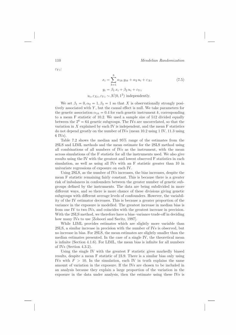
110 Mendelian Randomization
εY i:
xi =
6∑
k=1
α1k gik + α2 ui + εXi (7.5)
yi = β1 xi + β2 ui + εY i
ui, εXi, εY i ∼ N (0, 12) independently.
We set β1 = 0, α2 = 1, β2 = 1 so that X is observationally strongly posi-tively associated with Y , but the causal effect is null. We take parameters forthe genetic association α1k = 0.4 for each genetic instrument k, correspondingto a mean F statistic of 10.2. We used a sample size of 512 divided equallybetween the 26 = 64 genetic subgroups. The IVs are uncorrelated, so that thevariation in X explained by each IV is independent, and the mean F statisticsdo not depend greatly on the number of IVs (mean 10.2 using 1 IV, 11.3 using6 IVs).
Table 7.2 shows the median and 95% range of the estimates from the2SLS and LIML methods and the mean estimate for the 2SLS method usingall combinations of all numbers of IVs as the instrument, with the meanacross simulations of the F statistic for all the instruments used. We also giveresults using the IV with the greatest and lowest observed F statistics in eachsimulation, as well as using all IVs with an F statistic greater than 10 inunivariate regressions of exposure on each IV.
Using 2SLS, as the number of IVs increases, the bias increases, despite themean F statistic remaining fairly constant. This is because there is a greaterrisk of imbalances in confounders between the greater number of genetic sub-groups defined by the instruments. The data are being subdivided in moredifferent ways, and so there is more chance of these divisions giving geneticsubgroups with different average levels of confounders. However, the variabil-ity of the IV estimator decreases. This is because a greater proportion of thevariance in the exposure is modelled. The greatest increase in median bias isfrom one IV to two IVs, and coincides with the greatest increase in precision.With the 2SLS method, we therefore have a bias–variance trade-off in decidinghow many IVs to use [Zohoori and Savitz, 1997].
While LIML provides estimates which are slightly more variable than2SLS, a similar increase in precision with the number of IVs is observed, butno increase in bias. For 2SLS, the mean estimates are slightly smaller than themedian estimates presented. In the case of a single IV, the theoretical meanis infinite (Section 4.1.6). For LIML, the mean bias is infinite for all numbersof IVs (Section 4.3.2).
Using the single IV with the greatest F statistic gives markedly biasedresults, despite a mean F statistic of 23.9. There is a similar bias only usingIVs with F > 10. In the simulation, each IV in truth explains the sameamount of variation in the exposure. If the IVs are chosen to be included inan analysis because they explain a large proportion of the variation in theexposure in the data under analysis, then the estimate using these IVs is

Weak instruments and finite-sample bias 111
additionally biased. This is because the IVs explaining the most variation willbe overestimating the proportion of true variation explained, due to chancecorrelation with confounders. In the notation of Section 7.3.1, ∆U is largeand, having the same sign as α1, leads to an estimate biased in the directionof β2
α2
. Conversely, if the IV with the least F statistic is used as an instrument,the IV estimator will be biased in the opposite direction to the observationalassociation, as shown in Table 7.2.
So we see that if the F statistic is used either to choose between instru-ments, or via a rule such as only including an IV in the analysis if F > 10, thisprocedure itself introduces a selection bias which can be greater in magnitudethan the bias from weak instruments [Hall et al., 1996]. In a more realisticexample, IVs would not all have the same true strength. However, the largesampling variation in F statistics means that choosing between IVs on thebasis of a single measured F statistic is unreliable. One solution to this inpractice is to use the strength of the IVs in an independent dataset to de-termine the IVs to include in an applied analysis, or to use an allele score tosummarize multiple variants as a single IV (see Chapter 8).
Median 2.5% to 97.5% quantiles Mean Mean F
IVs used 2SLS LIML 2SLS 1 statistic
1 IV 0.00 −1.12 to 0.53 − 10.2
2 IVs 0.02 −0.54 to 0.39 0.00 −0.64 to 0.39 0.00 10.4
3 IVs 0.03 −0.39 to 0.33 0.00 −0.48 to 0.32 0.02 10.6
4 IVs 0.03 −0.31 to 0.30 0.00 −0.40 to 0.28 0.02 10.8
5 IVs 0.04 −0.26 to 0.27 0.00 −0.34 to 0.26 0.03 11.0
6 IVs 0.04 −0.23 to 0.26 0.00 −0.31 to 0.23 0.03 11.3
Greatest F 0.14 −0.30 to 0.52 − 23.9
Least F −0.32 −2.57 to 0.58 − 6.7
IVs with F > 10 0.11 −0.20 to 0.39 0.10 −0.22 to 0.39 0.11 16.4
TABLE 7.2
Evaluation of bias: Median and 95% range of estimates of β1 = 0 using 2SLS
and LIML methods, mean estimate using 2SLS method and mean F statistic
across 100 000 simulations using combinations of six uncorrelated instruments,
using the instrument with the greatest/least F statistic, and using all instru-
ments with univariate F statistics greater than 10.
1Mean estimate is reported only when it is not theoretically infinite
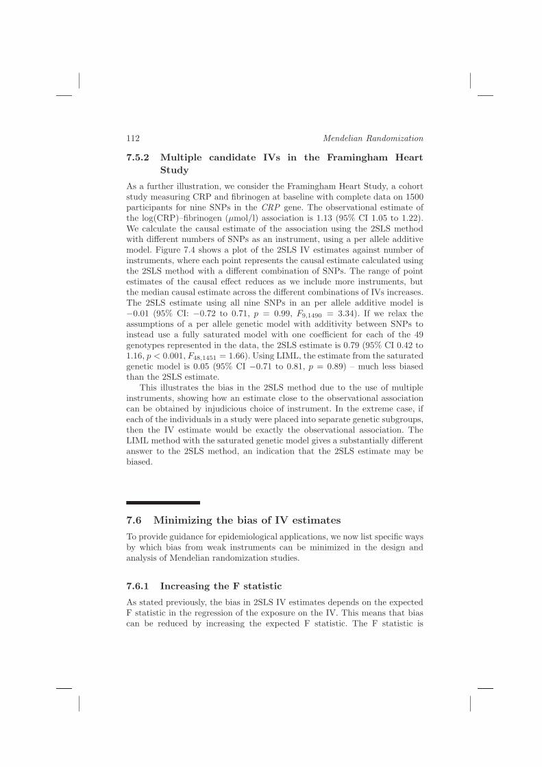
112 Mendelian Randomization
7.5.2 Multiple candidate IVs in the Framingham Heart
Study
As a further illustration, we consider the Framingham Heart Study, a cohortstudy measuring CRP and fibrinogen at baseline with complete data on 1500participants for nine SNPs in the CRP gene. The observational estimate ofthe log(CRP)–fibrinogen (µmol/l) association is 1.13 (95% CI 1.05 to 1.22).We calculate the causal estimate of the association using the 2SLS methodwith different numbers of SNPs as an instrument, using a per allele additivemodel. Figure 7.4 shows a plot of the 2SLS IV estimates against number ofinstruments, where each point represents the causal estimate calculated usingthe 2SLS method with a different combination of SNPs. The range of pointestimates of the causal effect reduces as we include more instruments, butthe median causal estimate across the different combinations of IVs increases.The 2SLS estimate using all nine SNPs in an per allele additive model is−0.01 (95% CI: −0.72 to 0.71, p = 0.99, F9,1490 = 3.34). If we relax theassumptions of a per allele genetic model with additivity between SNPs toinstead use a fully saturated model with one coefficient for each of the 49genotypes represented in the data, the 2SLS estimate is 0.79 (95% CI 0.42 to1.16, p < 0.001, F48,1451 = 1.66). Using LIML, the estimate from the saturatedgenetic model is 0.05 (95% CI −0.71 to 0.81, p = 0.89) – much less biasedthan the 2SLS estimate.
This illustrates the bias in the 2SLS method due to the use of multipleinstruments, showing how an estimate close to the observational associationcan be obtained by injudicious choice of instrument. In the extreme case, ifeach of the individuals in a study were placed into separate genetic subgroups,then the IV estimate would be exactly the observational association. TheLIML method with the saturated genetic model gives a substantially differentanswer to the 2SLS method, an indication that the 2SLS estimate may bebiased.
7.6 Minimizing the bias of IV estimates
To provide guidance for epidemiological applications, we now list specific waysby which bias from weak instruments can be minimized in the design andanalysis of Mendelian randomization studies.
7.6.1 Increasing the F statistic
As stated previously, the bias in 2SLS IV estimates depends on the expectedF statistic in the regression of the exposure on the IV. This means that biascan be reduced by increasing the expected F statistic. The F statistic is
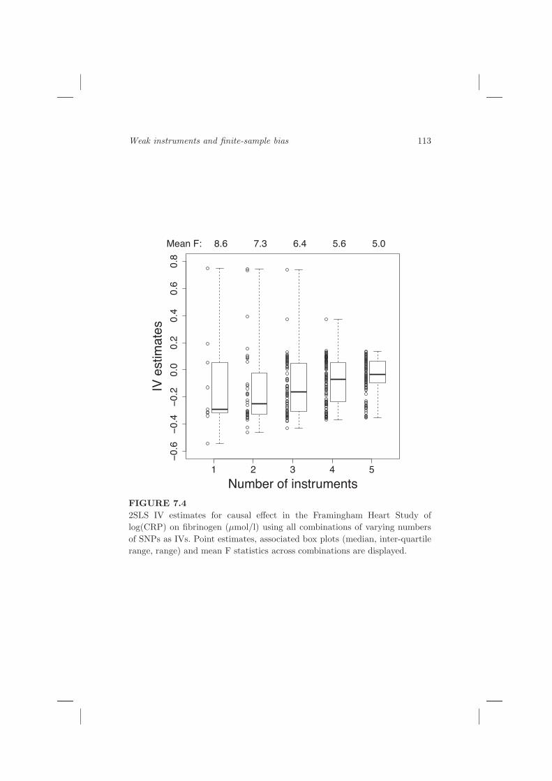
Weak instruments and finite-sample bias 113
1 2 3 4 5
−0.6
−0.4
−0.2
0.0
0.2
0.4
0.6
0.8
Number of instruments
IV estimates
Mean F: 8.6 7.3 6.4 5.6 5.0
FIGURE 7.4
2SLS IV estimates for causal effect in the Framingham Heart Study of
log(CRP) on fibrinogen (µmol/l) using all combinations of varying numbers
of SNPs as IVs. Point estimates, associated box plots (median, inter-quartile
range, range) and mean F statistics across combinations are displayed.

114 Mendelian Randomization
related to the proportion of variance in the exposure explained by the ge-netic variants (R2), sample size (N) and number of instruments (K) by the
formula F = (N−K−1
K) ( R2
1−R2 ). As the F statistic depends on the sample size,bias can be reduced by increasing the sample size. Similarly, if there are in-struments that are not contributing much to explaining the variation in theexposure, then excluding these instruments will increase the F statistic. Ingeneral, employing fewer degrees of freedom to model the genetic association,that is using parsimonious models, will increase the F statistic and reduceweak instrument bias, provided that the model does not misrepresent thedata [Pierce et al., 2011; Palmer et al., 2011a]. Simulations have shown that,even when the true model is only approximately linear in the IV, a per allelegenetic model reduces bias [Burgess and Thompson, 2011].
However, it is not enough to simply rely on an F statistic measured fromdata to inform us about bias [Hall et al., 1996]. Returning to the example fromSection 7.2.1 where we divided the Copenhagen General Population Study into16 equally sized substudies with mean F statistic 10.8, Figure 7.5 shows theestimates of these 16 substudies using the 2SLS method with their correspond-ing F statistics. We see that the substudies which have greater estimates arethe ones with larger F statistics; the correlation between F statistics and pointestimates is 0.83. The substudies with higher F statistics also have tighter CIsand so receive more weight in the meta-analysis. If we exclude from the meta-analysis substudies with an F statistic less than 10, then the pooled estimateincreases from 0.23 (SE 0.14, p = 0.09) to 0.43 (SE 0.16, p = 0.006). Equally,if we only use as instruments in each substudy the IVs with an F statisticgreater than 10 when regressed in a univariate regression on the exposure,then the pooled estimate increases to 0.28 (SE 0.15, p = 0.06). So neither ofthese approaches are useful in reducing bias.
Although the expectation of the F statistic is a good indicator of bias,the observed F statistic shows considerable variation. In the 16 substudies ofFigure 7.5, the measured F statistic ranges from 3.4 to 22.6. In more realisticexamples, assuming similar instruments in each study, larger studies wouldhave higher expected F statistics which would correspond to truly strongerinstruments and less bias. However, the sampling variation of causal effectsand observed F statistics in each study would still tend to follow the patternof Figure 7.5, with larger observed F statistics corresponding to more biasedcausal estimates.
So while it is desirable to use strong instruments, the measured strengthof instruments in data is not a good guide to the true instrument strength.Echoing the comments of Section 7.5 regarding the inclusion of IVs in a model,any guidance that relies on providing a threshold (such as F > 10) as aninclusion criterion is flawed and may introduce more bias than it prevents.

Weak instruments and finite-sample bias 115
−3.0 −1.8 −0.6 0.4 1.4
0.23 ( −0.04 , 0.50 )
−0.91 ( −2.90 , 1.08 )
−0.80 ( −2.54 , 0.93 )
−0.67 ( −2.04 , 0.70 )
−0.44 ( −2.61 , 1.73 )
−0.41 ( −1.77 , 0.95 )
−0.27 ( −1.64 , 1.10 )
−0.14 ( −1.98 , 1.69 )
−0.12 ( −1.11 , 0.87 )
−0.01 ( −1.28 , 1.26 )
0.02 ( −1.06 , 1.10 )
0.05 ( −0.87 , 0.97 )
0.18 ( −0.95 , 1.32 )
0.33 ( −0.65 , 1.30 )
0.59 ( −0.22 , 1.40 )
0.74 ( 0.05 , 1.42 )
0.83 ( 0.11 , 1.54 )
Study
F statistic: 4.4
F statistic: 5.9
F statistic: 8.6
F statistic: 3.4
F statistic: 8.2
F statistic: 6.9
F statistic: 4.2
F statistic: 14.2
F statistic: 7.4
F statistic: 11.4
F statistic: 16.5
F statistic: 10.4
F statistic: 12.4
F statistic: 17.2
F statistic: 22.6
F statistic: 19.4
Pooled estimate
Effect (95% CI)
FIGURE 7.5
Forest plot of causal estimates of log(CRP) on fibrinogen (µmol/l) using data
from the Copenhagen General Population Study divided randomly into 16
equally sized substudies (each N ≃ 2230). Studies ordered by causal esti-
mate. F statistic from regression of exposure on three IVs. Size of markers is
proportional to weight in a fixed-effect meta-analysis.

116 Mendelian Randomization
7.6.2 Adjustment for measured covariates
If we can find measured covariates that explain variation in the exposure, andthat are not on the causal pathway between exposure and outcome, then wecan incorporate these covariates in our model. This will increase precision inthe genetic association with the exposure and reduce weak instrument bias.Simulations have shown that we may also see an increase in the precision ofthe IV estimator if these covariates are additionally used to explain variationin the outcome [Burgess et al., 2011b].
As an example, we consider data on interleukin-6 (IL6), a cytokine which isinvolved in the inflammation process upstream of CRP and fibrinogen [Hans-son, 2005]. Elevated levels of IL6 lead to elevated levels of both CRP andfibrinogen, so IL6 is correlated with short-term variation in CRP [Kaptoge etal., 2010], but is independent of underlying genetic variation in CRP [CCGC,2011]. We assume that it is a confounder in the association of CRP with fib-rinogen and not on the causal pathway (if such a pathway exists). As IL6 hasa positively skewed distribution, we take its logarithm.
We use data from the Cardiovascular Health Study, a cohort study fromthe CCGC measuring CRP, IL6 and fibrinogen at baseline, as well as threeSNPs (rs1205, rs1417938, and rs1800947) on the CRP gene, with completedata for 4137 subjects. The proportion of variance in log(CRP) explained bylog(IL6) is 26%. We calculate the 2SLS IV estimate of the CRP–fibrinogen as-sociation for each SNP separately and for all the SNPs together in an per alleleadditive model, both without and with adjustment for log(IL6) in the first-and second-stage regressions. Results are given in Table 7.3. We see that afteradjusting for log(IL6) the causal estimate in each case has decreased (reflect-ing reduced weak instrument bias), its standard error has reduced (reflectingincreased precision), and the F statistic has increased. With adjustment fora covariate, the relevant F statistic is a partial F statistic, representing thevariation in the exposure explained by the IVs once the variation explainedby the covariate has been accounted for. This is calculated from an analysisof variance (ANOVA) model.
7.6.3 Borrowing information across studies
The IV estimator would be unbiased if we knew the true values for the averageexposure in different genetic subgroups. In a meta-analysis context [Thompsonet al., 2005], we can combine the estimates of genotype–exposure associationfrom different studies to give more precise estimates of exposure levels in eachgenetic subgroup. In the 2SLS method, an individual participant data (IPD)fixed-effect meta-analysis for data on individual i in study m with exposurexim, outcome yim and gikm for number of minor alleles (0, 1, or 2) of genetic

Weak instruments and finite-sample bias 117
Not adjusted Adjusted
IV estimate Estimate (SE) F statistic Estimate (SE) F statistic
Using rs1205 0.219 (0.201) 79.6 0.173 (0.196) 100.2
Using rs1417938 −0.457 (0.407) 27.6 −0.458 (0.362) 37.2
Using rs1800947 0.354 (0.325) 28.6 0.324 (0.316) 36.5
Using all 3 SNPs 0.186 (0.194) 24.4 0.127 (0.188) 32.2
TABLE 7.3
2SLS estimates and standard errors (SE) of the causal effect of log(CRP)
on fibrinogen, and F statistic for regression of log(CRP) on IVs, calculated
using each SNP separately and all SNPs together in per allele additive model,
without and with adjustment for log(IL6) in the Cardiovascular Health Study.
variant k (k = 1, 2, . . .Km) is:
xim = α0m +
Km∑
k=1
αkm gikm + εXim (7.6)
yim = β0m + β1 xim + εY im
εXim ∼ N (0, σ2
X); εY im ∼ N (0, σ2
Y ) independently.
The exposure levels are regressed on the IVs using a per allele additive linearmodel separately in each study, and then the outcome levels are regressed onthe fitted values of exposure (xim). The terms α0m and β0m are study-specificintercept terms. Here we assume homogeneity of variances across studies; wecan use Bayesian methods to allow for possible heterogeneity (see Section 9.6).
If the same genetic variants are measured in each study and are assumedto have the same effect on the exposure, we can use common genetic effects(i.e. αkm = αk) across studies by replacing the first line in equation (7.6) with:
xim = α0m +
K∑
k=1
αk gikm + εXim (7.7)
If the assumption of common genetic effects is correct, this will improve theprecision of the fitted values (xim) and reduce weak instrument bias.
To illustrate this, we consider the Copenhagen City Heart Study (CCHS),Edinburgh Artery Study (EAS), Health Professionals Follow-up Study(HPFS), Nurses Health Study (NHS), and Stockholm Heart EpidemiologyProgram (SHEEP), which are cohort studies or case-control studies measuringCRP and fibrinogen levels at baseline [CCGC, 2008]. In case-control studies,we use the data from controls alone since these better represent cross-sectionalpopulation studies. These five studies measured the same three SNPs on theCRP gene: rs1205, rs1130864 and rs3093077 (or rs3093064, which is in com-plete linkage disequilibrium with rs3093077). We estimate the causal effect

118 Mendelian Randomization
Causal Observational
Study N F df estimate (SE) estimate (SE)
CCHS 7999 29.6 (3, 7995) −0.286 (0.373) 1.998 (0.030)
EAS 650 6.9 (3, 646) 0.754 (0.327) 1.115 (0.056)
HPFS 405 5.3 (3, 401) 0.758 (0.423) 1.048 (0.081)
NHS 385 6.1 (3, 381) −0.906 (0.636) 0.562 (0.114)
SHEEP 1044 10.5 (3, 1040) 0.088 (0.345) 1.078 (0.051)
Different genetic effects 14.4 (15, 10463) 0.021 (0.195)
Common genetic effects 56.6 ( 3, 10475) −0.093 (0.225)
Study-level estimates 0.234 (0.174)
TABLE 7.4
Estimates of effect of log(CRP) on fibrinogen (µmol/l) from each of five stud-
ies separately and from meta-analysis of studies: number of participants (N),
F statistic (F ) with degrees of freedom (df) from per allele additive regression
of exposure on three SNPs used as IVs, causal estimate using 2SLS with stan-
dard error (SE), observational estimate with SE. Fixed-effect meta-analyses
conducted using individual-level data with different study-level genetic ef-
fects, common pooled genetic effects, and combining study-level estimates
with inverse-variance weighting.
using the 2SLS method with different genetic effects (model 7.6), common ge-netic effects (model 7.7) and by a fixed-effect meta-analysis of estimates fromeach study.
Table 7.4 shows that the studies analysed separately have apparently dis-parate causal estimates with large SEs. The meta-analysis estimate assumingcommon genetic effects across studies is further from the confounded observa-tional estimates and closer to the IV estimate from the largest study with thestrongest instruments (CCHS) than the model with different genetic effects,suggesting that the latter suffers bias from weak instruments.
The pooled estimate from the study-level meta-analysis is greater thanthose from the individual-level meta-analyses. Although the CCHS study hasabout 8 times the number of participants as SHEEP and 12 times as many asEAS, its causal estimate has a larger standard error. The standard errors inthe 2SLS method are known to be underestimated when the correlation due toconfounding is strong, especially with weak instruments (Section 7.4.2) [Stockand Yogo, 2002]. Also, Figure 7.5 showed that causal estimates nearer to theobservational association have lower variance. So a study-level meta-analysismay be biased due to overestimated weights in the studies with more biasedestimates.
Returning to the example of data from the Copenhagen General Popu-lation Study considered in Section 7.2.1, if we use the IPD (model 7.6) to

Weak instruments and finite-sample bias 119
Different Common
genetic genetic
Substudies Meta-analysis p-value effects p-value effects p-value
1 −0.05 (0.15) 0.76
5 −0.01 (0.15) 0.95 −0.03 (0.15) 0.85 −0.05 (0.15) 0.75
10 0.09 (0.14) 0.54 0.04 (0.14) 0.80 −0.05 (0.15) 0.76
16 0.23 (0.14) 0.09 0.15 (0.14) 0.26 −0.05 (0.15) 0.75
40 0.46 (0.13) < 0.001 0.30 (0.13) 0.02 −0.04 (0.15) 0.77
100 0.83 (0.11) < 0.001 0.68 (0.11) < 0.001 −0.04 (0.15) 0.77
250 1.27 (0.08) < 0.001 1.15 (0.08) < 0.001 −0.04 (0.15) 0.78
TABLE 7.5
2SLS estimates of causal effect (standard error) of log(CRP) on fibrinogen
from the Copenhagen General Population Study divided randomly into sub-
studies and combined: using fixed-effect meta-analysis of substudy estimates,
and using individual patient data (IPD) with different or common genetic
effects across substudies.
combine the substudies in the meta-analysis rather than combining estimatesfrom each substudy, then the pooled estimates are somewhat less biased (Ta-ble 7.5). If we additionally assume common genetic effects across studies(model 7.7), then we recover close to the original estimate based on analysingthe full dataset as one study: weak instrument bias has been eliminated.
7.7 Discussion
This chapter has demonstrated the effect of weak instrument bias on causalestimates in real and simulated data. The magnitude of this bias depends onthe statistical strength of the association between instrument and exposure.
Weak instrument bias can reintroduce the problem that IVs were developedto solve. It is misleading not solely because it biases estimates, but becauseestimates suffering from the bias do not provide a valid test of the null hy-pothesis. Weak instruments may convince a researcher that an observationalassociation that they have estimated is in fact causal. The reason for the biasis that the variation in the exposure explained by the IV is not large enough todominate the variation in the exposure caused by chance correlation betweenthe IV and confounders.
While the magnitude of the bias depends on the instrument strengththrough the expected or mean F statistic, for a study of fixed size and under-lying instrument strength, an observed F statistic greater than its expectedvalue corresponds to an estimate closer to the observational association with

120 Mendelian Randomization
greater precision; conversely an observed F statistic less than the expectedvalue corresponds with an estimate further from the observational associationwith less precision. Simply relying on an F statistic from an individual studyis over-simplistic and threshold rules such as ensuring F > 10 may cause morebias than they prevent.
7.7.1 Bias–variance trade-off
Using the 2SLS method, we demonstrated a bias–variance trade-off for thenumber of instruments used in IV estimation. For a fixed mean F statistic,as the number of instruments increases, the precision of the IV estimatorincreases, but the bias also increases. Using the LIML method, bias did notincrease with the number of instruments, but the precision was slightly lowerthan for 2SLS. When using 2SLS, we seek parsimonious models of geneticassociation, for example using per allele additive models and including onlyIVs with a known association with the exposure, based on biological knowledgeand external information. Provided the data are not severely misrepresented,these should provide the best estimates of the causal effect. Again, post hocuse of observed F statistics to choose between instruments may cause morebias than it prevents.
7.7.2 Combatting weak instrument bias in practice
Ideally, issues of weak instrument bias should be addressed prior to data col-lection, by specifying sample sizes, instruments, and genetic models using thebest prior evidence available, to ensure that the expected values of F statis-tics are large. Where this is not possible, our advice would be to conductsensitivity analyses using different IV methods, numbers of instruments andgenetic models to investigate the impact of different assumptions on the causalestimate.
Testing the association between the outcome and each IV in turn (withoutestimating a causal effect) is a valid test of a causal relationship even withweak instruments. If there is a single IV, then an expected F statistic of 5corresponds to a p-value in the regression of the exposure on the IV of around0.03. It is perhaps unlikely that an IV would be considered for use in a datasetif the expected p-value were much greater than 0.03, and so bias from weakinstruments would not be expected to be an issue in practice with a singleIV. If there are multiple IVs, LIML or Bayesian methods could be used in theanalysis, as the estimates from these are less biased than the 2SLS estimate.A difference between the 2SLS and LIML IV estimates is evidence of possiblebias from weak instruments. The use of Fieller’s theorem, the Anderson–Rubintest statistic or a Bayesian posterior distribution for inference is recommended.
It is also possible to summarize multiple SNPs into a single variable toreduce weak instrument bias using an allele score. Details about how to con-struct such a score are given in Chapter 8.
Weak instruments and finite-sample bias 121
Adjustment for covariates helps reduce weak instrument bias. Includingpredictors of the exposure in the first-stage regression, or predictors of theoutcome in the second-stage regression, also increases precision of the causalestimate. The former will also increase the F statistic for the IVs, and thusreduce weak instrument bias.
This chapter has considered bias in a one-sample Mendelian randomiza-tion setting. If the genetic associations with the exposure and outcome areestimated in non-overlapping sets of individuals, then bias from weak instru-ments will act in the direction of the null (Section 9.8.2). Although bias isnever welcome, the direction of bias in a two-sample Mendelian randomiza-tion analysis means that a non-null causal effect estimate will not simply bean artefact of weak instrument bias.
7.7.3 Bias in study-level meta-analysis
In a meta-analysis context, bias is a more serious issue, as it arises not onlyfrom the bias in the individual studies, but also from the correlation betweencausal effect estimates and their variances which results in studies with effectscloser to the observational estimate being over-weighted. By using a singleIPD model, we can reduce the second source of bias. Additionally, we canpool information on the genetic association across studies to strengthen theinstruments. The assumptions of homogeneity of variances and common ge-netic effects across studies made in Section 7.6.3 are overly restrictive in prac-tice; more reasonable extensions of IV methods to a meta-analysis context arediscussed in Chapter 9.
7.7.4 Caution about validity of IVs
Finally, we recall that the use of a genetic instrument in Mendelian randomiza-tion relies on certain assumptions. In this chapter we have assumed, althoughthese may fail in finite samples, that they hold asymptotically. If these as-sumptions do not hold, for example if there were a true correlation betweenthe instrument and a confounder, then IV estimates can be entirely misleading[Small and Rosenbaum, 2008].
7.8 Key points from chapter
• Bias from weak instruments can result in seriously misleading estimates ofcausal effects. Studies with instruments having large expected F statisticsare less biased on average. However, if a study by chance has a larger
122 Mendelian Randomization
observed F statistic than expected, then the causal estimate will be morebiased.
• Coverage levels with weak instruments can be poorly estimated by methodswhich rely on assumptions of asymptotic normality.
• Data-driven choice of instruments or analysis can exacerbate bias. In partic-ular, any threshold guideline such as ensuring that an observed F statisticis greater than 10 is misleading. Methods, instruments, and data to beused should be specified prior to data analysis. Meta-analyses based onstudy-specific estimates of causal effect are susceptible to bias.
• Bias can be alleviated by use of measured covariates and parsimoniousmodelling of the genetic association (such as a per allele additive SNPmodel rather than one coefficient per genotype). This should be accom-panied by sensitivity analyses to assess potential bias, for example frommodel misspecification.
• Bias can be reduced substantially by using LIML, Bayesian and allele score(see next chapter) methods rather than 2SLS, and bias in practice with asingle IV should be minimal. Nominal coverage levels can be maintainedby the use of Fieller’s theorem with a single IV, and confidence intervalsfrom the Anderson–Rubin test statistic or Bayesian MCMC methods withmultiple IVs.


![Parameter-free, weak imposition of Dirichlet …WEAK COUPLING OF TRIMMED PATCHES 671 the finite cell method [3, 4], an embedded domain method of high order, which is also applicable](https://img.dokumen.tips/doc/110x75/5f4f08abec270a77940dd887/parameter-free-weak-imposition-of-dirichlet-weak-coupling-of-trimmed-patches-671.jpg)