Weak instruments - London School of Economics and ...econ.lse.ac.uk/staff/spischke/ec533/Weak IV.pdfIV regression with weak instruments Bound, Jaeger, and Baker (1995) pointed out

Weak instruments

Jörn-Steffen Pischke

LSE

October 14, 2016

Pischke (LSE) Weak instruments October 14, 2016 1 / 25

IV regression with weak instruments

Bound, Jaeger, and Baker (1995) pointed out that the quarter of birthinstruments explain only a tiny proportion of the variation in schooling.This leads to two distinct problems:

The 2SLS estimator with weak instruments is biased in small samples.

Any inconsisency from a small violation of the exclusion restrictiongets magnified by weak instruments.


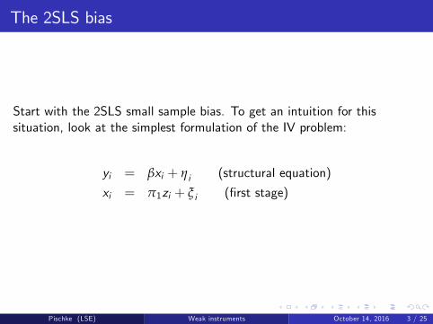
The 2SLS bias

Start with the 2SLS small sample bias. To get an intuition for thissituation, look at the simplest formulation of the IV problem:

yi = βxi + ηi (structural equation)

xi = π1zi + ξ i (first stage)


The small sample behavior with one instrument

If an instrument is basically irrelevant then π1 ≈ 0. Recall

βIV =cov (yi , zi )cov (xi , zi )

butcov (xi , zi ) = cov (π1zi + ξ i , zi ) = π1σ

2Z

So if π1 = 0,cov (xi , zi ) = 0

and the IV estimator doesn’t exist.

Even when π1 is truely zero, in any finite sample the sample analogueto cov (xi , zi ) will not be exactly zero. But this is of little comfort asthe sampling variation in cov (xi , zi ) is not helpful to estimate β.


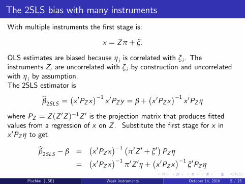
The 2SLS bias with many instruments

With multiple instruments the first stage is:

x = Zπ + ξ.

OLS estimates are biased because ηi is correlated with ξ i . Theinstruments Zi are uncorrelated with ξ i by construction and uncorrelatedwith ηi by assumption.The 2SLS estimator is

β̂2SLS =(x ′PZ x

)−1 x ′PZ y = β+(x ′PZ x

)−1 x ′PZ η

where PZ = Z (Z ′Z )−1Z ′ is the projection matrix that produces fittedvalues from a regression of x on Z . Substitute the first stage for x inx ′PZ η to get

β̂2SLS − β =(x ′PZ x

)−1 (π′Z ′ + ξ ′

)PZ η

=(x ′PZ x

)−1π′Z ′η +

(x ′PZ x

)−1ξ ′PZ η


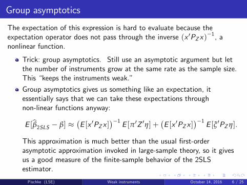
Group asymptotics

The expectation of this expression is hard to evaluate because theexpectation operator does not pass through the inverse (x ′PZ x)

−1, anonlinear function.

Trick: group asymptotics. Still use an asymptotic argument but letthe number of instruments grow at the same rate as the sample size.This “keeps the instruments weak.”

Group asymptotics gives us something like an expectation, itessentially says that we can take these expectations throughnon-linear functions anyway:

E [β̂2SLS − β] ≈(E [x ′PZ x ]

)−1 E [π′Z ′η] + (E [x ′PZ x ])−1 E [ξ ′PZ η].

This approximation is much better than the usual first-orderasymptotic approximation invoked in large-sample theory, so it givesus a good measure of the finite-sample behavior of the 2SLSestimator.



Remember the instruments Zi are uncorrelated with ξ i and ηi . ThereforeE [π′Z ′η] = 0, and we have

E [β̂2SLS − β] ≈(E [x ′PZ x ]

)−1 E [π′Z ′η] + (E [x ′PZ x ])−1 E [ξ ′PZ η]

=(E [x ′PZ x ]

)−1 E [ξ ′PZ η].

Substitute in the first stage again.

E [β̂2SLS − β] ≈(E [(π′Z ′ + ξ ′

)PZ (Zπ + ξ)]

)−1 E [ξ ′PZ η].

Note that E [π′Z ′ξ] = 0, so we get no cross-terms:

E [β̂2SLS − β] ≈[E(π′Z ′Zπ

)+ E (ξ ′PZ ξ)

]−1 E (ξ ′PZ η).



Matrix algebra trick: ξ ′PZ ξ is a scalar, therefore equal to its trace; thetrace is a linear operator which passes through expectations and isinvariant to cyclic permutations; finally, the trace of PZ , an idempotentmatrix, is equal to it’s rank, q. Using these facts

E(ξ ′PZ ξ

)= E

[tr(ξ ′PZ ξ

)]= E

[tr(PZ ξξ ′

)]= tr

(PZE

[ξξ ′])

= tr(PZ σ2ξ I

)= σ2ξtr (PZ )

= σ2ξq,

where we have assumed that ξ i is homoskedastic. Similarly, applying thetrace trick to ξ ′PZ η shows that this term is equal to σηξq.



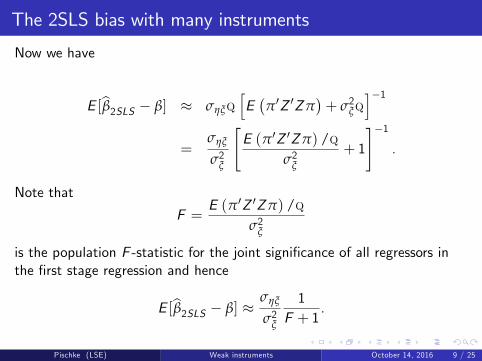
Now we have

E [β̂2SLS − β] ≈ σηξq[E(π′Z ′Zπ

)+ σ2ξq

]−1=

σηξ

σ2ξ

[E (π′Z ′Zπ) /q

σ2ξ+ 1

]−1.

Note that

F =E (π′Z ′Zπ) /q

σ2ξ

is the population F -statistic for the joint significance of all regressors inthe first stage regression and hence

E [β̂2SLS − β] ≈σηξ

σ2ξ

1F + 1

.


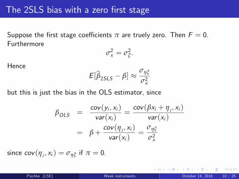
The 2SLS bias with a zero first stage

Suppose the first stage coeffi cients π are truely zero. Then F = 0.Furthermore

σ2x = σ2ξ .

HenceE [β̂2SLS − β] ≈

σηξ

σ2x

but this is just the bias in the OLS estimator, since

βOLS =cov(yi , xi )var(xi )

=cov(βxi + ηi , xi )

var(xi )

= β+cov(ηi , xi )var(xi )

=σηξ

σ2x

since cov(ηi , xi ) = σηξ if π = 0.


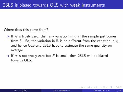
2SLS is biased towards OLS with weak instruments

Where does this come from?

If π is truely zero, then any variation in x̂i in the sample just comesfrom ξ i . So, the variation in x̂i is no different from the variation in xi ,and hence OLS and 2SLS have to estimate the same quantity onaverage.

If π is not truely zero but F is small, then 2SLS will be biasedtowards OLS.


What does the weak instrument bias depend on?

The weak instrument bias tends to get worse as we add more (weak)instruments. To see this consider

F =E (π′Z ′Zπ) /q

σ2ξ

Suppose you have some existing instruments, and you add new ones withno additional exploratory power. I.e. the π coeffi cients on the additionalinstruments will be zero.

π′Z ′Zπ will remain the same as before adding more instruments.

Since the first stage regression is unchanged by the additionalinstruments, σ2ξ will also remain the same.

q will go up.

As a result, F will go down, and the 2SLS bias will get worse.


Summing up on the bias

With weak instruments

2SLS is biased towards OLS.

The bias will tend to be worse when there are many overidentifyingrestrictions (many instruments compared to endogenous regressors).

Just identified IV is approximately unbiased (or less biased) even withweak instruments (although it is not possible to see this from the biasformula).

Estimated standard errors of 2SLS and IV estimators may be toosmall.


LIML

There are alternative estimators, which have better small sampleproperties than 2SLS with weak instruments. One such estimator isLIML (limited information maximum likelihood).

LIML is a linear combination of the OLS and 2SLS estimate (with theweights depending on the data), and the weights happen to be suchthat they (approximately) eliminate the 2SLS bias.


A Monte Carlo Experiment

Simulate data from the following model

yi = βxi + ηi

xi =Q

∑j=1

πjzij + ξ i

with β = 1, π1 = 0.1, πj = 0 for j = 2, ...,Q,(ηiξ i

)∣∣∣∣Z ∼ N (( 00

),

(1 0.80.8 1

)),

where the zij are independent, normally distributed random variables withmean zero and unit variance. The sample size is 1000.


Monte Carlo Results2SLS, LIML: 2 instruments, IV: one instrument

0.2

5.5

.75

1

0 .5 1 1.5 2 2.5x

OLS IV2SLS LIML


Monte Carlo Results20 instruments

0.2

5.5

.75

1

0 .5 1 1.5 2 2.5x

OLS 2SLSLIML


Monte Carlo Results20 garbage instruments

0.2

5.5

.75

1

0 .5 1 1.5 2 2.5x

OLS 2SLSLIML


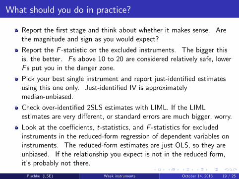
What should you do in practice?

Report the first stage and think about whether it makes sense. Arethe magnitude and sign as you would expect?

Report the F -statistic on the excluded instruments. The bigger thisis, the better. F s above 10 to 20 are considered relatively safe, lowerF s put you in the danger zone.

Pick your best single instrument and report just-identified estimatesusing this one only. Just-identified IV is approximatelymedian-unbiased.

Check over-identified 2SLS estimates with LIML. If the LIMLestimates are very different, or standard errors are much bigger, worry.

Look at the coeffi cients, t-statistics, and F -statistics for excludedinstruments in the reduced-form regression of dependent variables oninstruments. The reduced-form estimates are just OLS, so they areunbiased. If the relationship you expect is not in the reduced form,it’s probably not there.


Some alternative AK91 estimates

“38332_Angrist” — 10/18/2008 — 17:36 — page 214

−101

214 Chapter 4

Table 4.6.2Alternative IV estimates of the economic returns to schooling

(1) (2) (3) (4) (5) (6)

2SLS .105 .435 .089 .076 .093 .091(.020) (.450) (.016) (.029) (.009) (.011)

LIML .106 .539 .093 .081 .106 .110(.020) (.627) (.018) (.041) (.012) (.015)

F-statistic 32.27 .42 4.91 1.61 2.58 1.97(excluded instruments)

ControlsYear of birth � � � � � �State of birth � �Age, age squared � � �Excluded instrumentsQuarter-of-birth dummies � �Quarter of birth*year of birth � � � �Quarter of birth*state of birth � �Number of excluded instruments 3 2 30 28 180 178

Notes: The table compares 2SLS and LIML estimates using alternative sets of instru-ments and controls. The age and age squared variables measure age in quarters. The OLSestimate corresponding to the models reported in columns 1–4 is .071; the OLS estimatecorresponding to the models reported in columns 5 and 6 is .067. Data are from the Angristand Krueger (1991) 1980 census sample. The sample size is 329,509. Standard errors arereported in parentheses.

The first column in the table reports 2SLS and LIML esti-mates of a model using three quarter-of-birth dummies asinstruments, with year-of-birth dummies as covariates. TheOLS estimate for this specification is 0.071, while the 2SLSestimate is a bit higher, at 0.105. The first-stage F-statistic isover 32, well out of the danger zone. Not surprisingly, theLIML estimate is almost identical to 2SLS in this case.

Angrist and Krueger (1991) experimented with models thatinclude age and age squared measured in quarters as additionalcontrols. These controls are meant to pick up omitted ageeffects that might confound the quarter-of-birth instruments.The addition of age and age squared reduces the number ofinstruments to two, since age in quarters, year of birth, andquarter of birth are linearly dependent. As shown in column 2,the first-stage F-statistic drops to 0.4 when age and age squaredare included as controls, a sure sign of trouble. But the 2SLS


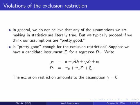
Violations of the exclusion restriction

In general, we do not believe that any of the assumptions we aremaking in statistics are literally true. But we typically proceed if wethink our assumptions are “pretty good.”

Is “pretty good”enough for the exclusion restriction? Suppose wehave a candidate instrument Zi for a regressor Di . Write

yi = α+ ρDi + γZi + eiDi = π0 + π1Zi + ξ i .

The exclusion restriction amounts to the assumption γ = 0.


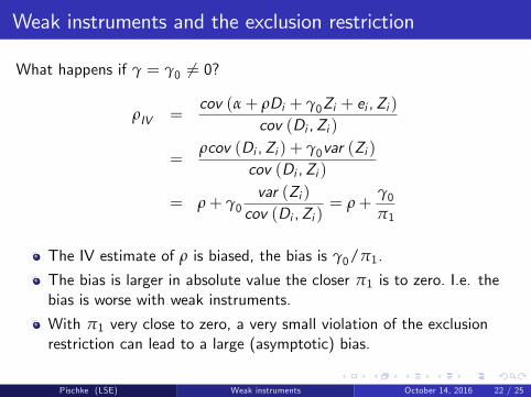
Weak instruments and the exclusion restriction

What happens if γ = γ0 6= 0?

ρIV =cov (α+ ρDi + γ0Zi + ei ,Zi )

cov (Di ,Zi )

=ρcov (Di ,Zi ) + γ0var (Zi )

cov (Di ,Zi )

= ρ+ γ0var (Zi )

cov (Di ,Zi )= ρ+

γ0π1

The IV estimate of ρ is biased, the bias is γ0/π1.

The bias is larger in absolute value the closer π1 is to zero. I.e. thebias is worse with weak instruments.

With π1 very close to zero, a very small violation of the exclusionrestriction can lead to a large (asymptotic) bias.


Can violation of the exclusion restriction explain AK91?

School starting age (SSA) is a candidate violation of the exclusionrestriction. Individuals born in quarter 4 start school younger.

The best paper on school starting age is Black, Devereux, andSalvanes, “Too Young to Leave the Nest?”REStat 2011 for Norway.They find an effect on log earnings of -0.1 at age 25, -0.01 (notsignificant) at age 30, 0.0 at age 35, suggesting SSA works throughlost labor market experience. (AK91 sample is in their 40s.)

To play with the numbers:

π1 = 0.09, this is the difference in schooling between quarter 4 andother quartersThose born in quarter 4 start school about 6 months younger, or -0.5of a year.γ0 is the effect of school starting age on earnings. Using the age 30 γ0of -0.01

γ0π1

=−0.01 ∗ −0.5

0.09= 0.055


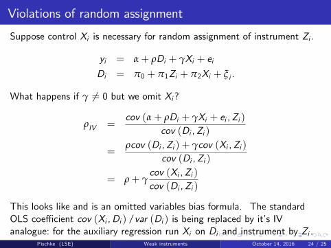
Violations of random assignment

Suppose control Xi is necessary for random assignment of instrument Zi .

yi = α+ ρDi + γXi + eiDi = π0 + π1Zi + π2Xi + ξ i .

What happens if γ 6= 0 but we omit Xi?

ρIV =cov (α+ ρDi + γXi + ei ,Zi )

cov (Di ,Zi )

=ρcov (Di ,Zi ) + γcov (Xi ,Zi )

cov (Di ,Zi )

= ρ+ γcov (Xi ,Zi )cov (Di ,Zi )

This looks like and is an omitted variables bias formula. The standardOLS coeffi cient cov (Xi ,Di ) /var (Di ) is being replaced by it’s IVanalogue: for the auxiliary regression run Xi on Di and instrument by Zi .


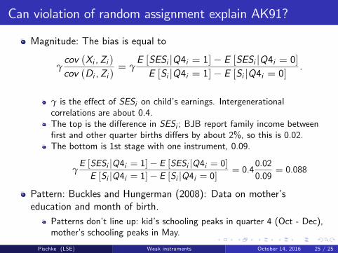
Can violation of random assignment explain AK91?

Magnitude: The bias is equal to

γcov (Xi ,Zi )cov (Di ,Zi )

= γE [SESi |Q4i = 1]− E [SESi |Q4i = 0]E [Si |Q4i = 1]− E [Si |Q4i = 0]

.

γ is the effect of SESi on child’s earnings. Intergenerationalcorrelations are about 0.4.The top is the difference in SESi ; BJB report family income betweenfirst and other quarter births differs by about 2%, so this is 0.02.The bottom is 1st stage with one instrument, 0.09.

γE [SESi |Q4i = 1]− E [SESi |Q4i = 0]E [Si |Q4i = 1]− E [Si |Q4i = 0]

= 0.40.020.09

= 0.088

Pattern: Buckles and Hungerman (2008): Data on mother’seducation and month of birth.

Patterns don’t line up: kid’s schooling peaks in quarter 4 (Oct - Dec),mother’s schooling peaks in May.


Documents

Weak instruments - London School of Economics and ...econ.lse.ac.uk/staff/spischke/ec533/Weak IV.pdfIV regression with weak instruments Bound, Jaeger, and Baker (1995) pointed out