On Bootstrap Validity for Specification Tests with Weak Instruments

Firmin Doko Tchatoka

Working Paper No. 2014-06 June, 2014

Copyright the authors

School of Economics

Working Papers ISSN 2203-6024

On bootstrap validity for specification tests with

weak instruments

Firmin Doko Tchatoka∗

The University of Adelaide

June 19, 2014

∗ School of Economics, The University of Adelaide, 10 Pulteney Street, Adelaide SA 5005, Tel:+6188313 5540, Fax:+618 8223 1460, e-mail: firmin.dokotchatoka@adelaide.edu.au

ABSTRACT

We investigate the asymptotic validity of the bootstrap forDurbin-Wu-Hausman (DWH)

tests of exogeneity in linear IV regressions, with or without identification. Our analysis

of the properties (size and power) of the proposed bootstraptests provides some new in-

sights and extensions of earlier studies. More precisely, we show that when identification

is strong, the bootstrap: (1) provides an asymptotic refinement of the size of the DWH tests

under exogeneity, and (2) is consistent under the alternative hypothesis if the endogeneity

parameter is fixed. However, the bootstrap only provides a first-order approximation of the

asymptotic distributions of these statistics when instruments are weak. Moreover, we char-

acterize the necessary and sufficient condition under whichthe proposed bootstrap DWH

tests exhibit power under fixed endogeneity and weak instruments. The latter condition

may still hold over a wide range of cases, provided that at least one instrument is not irrel-

evant. But all bootstrap tests have low power when all instruments are irrelevant, a case of

little interest in empirical work. We present a Monte Carlo experiment that confirms our

theoretical findings.

Key words: Exogeneity testing; Durbin-Wu-Hausman tests; weak instruments; bootstrap

validity; asymptotic refinement.

JEL classification: C3; C12; C15; C52.

i

1. Introduction

Exogeneity tests of the type proposed by Durbin (1954), Wu (1973, 1974), and Hausman

(1978), henceforth DWH tests, are widely used in applied work to determine whether or-

dinary least squares (OLS) or instrumental variables (IVs)method is appropriate. There is

now a considerable body of research1 on this topic, and most studies often impose iden-

tifying assumptions on model coefficients, thus leaving outissues associated withweak

instruments. It is well known that IV estimators can be imprecise and thatinference proce-

dures (such as tests and confidence sets) can be highly unreliable in the presence of weak

instruments. In recent years, concerns have been raised about the reliability of DWH pro-

cedures in the presence of weak instruments because they mainly rely on IV estimators.2

Staiger and Stock (1997) show that the limiting distributions of Hausman (1978) type

statistics depend on the concentration matrix, which usually determines the strength of the

identification. Meanwhile, Wu (1973, 1974)T2 andT4 statistics are asymptotically pivotal

under exogeneity even when identification is weak. Doko Tchatoka and Dufour (2011b)

provide a characterization of the finite-sample distributions of DWH statistics, allowing for

the possibility of identification failure and non-Gaussianerrors. They show that the statis-

tics T1, T2, andT4 by Wu (1973, 1974) are pivotal under exogeneity without identifying

assumptions, even when the errors are non-Gaussian. However, Wu (1973, 1974)T3 and

alternative Hausman (1978) type statistics do not share this property, but they are bound-

edly pivotal with or without non-Gaussian errors, no matterhow weak the instruments are.

This suggests that all DWH tests are valid (in the sense that their level is controlled) in the

presence of weak instruments if the usualF or asymptoticχ2 critical values are applied in

the inference. However, when applying the asymptoticχ2 critical values, Wu (1973, 1974)

1For examples, see Revankar and Hartley (1973), Farebrother(1976), Revankar (1978), Dufour (1987),Hwang (1980, 1985), Kariya and Hodoshima (1980), Nakamura and Nakamura (1981), Engle (1982), Holly(1982), Reynolds (1982), and Smith (1984, 1985, 1987), among others.

2For examples, see Staiger and Stock (1997), Wong (1996, 1997), Guggenberger (2010), Hahn, Ham andMoon (2010), Doko Tchatoka and Dufour (2011a, 2011b, 2014),Kiviet and Niemczyk (2007, 2012), andKiviet and Pleus (2012), among others.

1

T3 and Hausman (1978) statistic can lead to overly conservative procedures when identifi-

cation is weak. Size correction of the latter statistics is nonetheless achievable by resorting

to the exact Monte Carlo tests method such as in Dufour (2006)[see Doko Tchatoka and

Dufour (2011b)]. However, the proposed Monte Carlo method requires that the conditional

distribution of the structural disturbance, given the instruments, be specified, at least up to

an unknown scalar factor. In many empirical applications, researchers usually do not know

the distribution of the errors even conditionally on available instruments. So, implement-

ing the exact Monte Carlo tests can be difficult. Therefore, providing a distributional-free

method to improve the size and power of the DWH tests, especially when identification

is not very strong, can be of great interest in applied work. This paper attempts to make

progress in this direction.

To be more specific, we propose a bootstrap method for DWH exogeneity statistics that

is robust to identifying assumptions and does not require any distributional assumption on

model errors. To do this, we exploit the score interpretation of these statistics [see En-

gle (1982) and Smith (1983)] to suggest a bootstrap method similar to those of Moreira,

Porter and Suarez (2009).3 We provide an analysis of the limiting distributions of the pro-

posed bootstrap DWH statistics under both the null hypothesis (size) and the alternative

hypothesis (power), with or without weak instruments. Our results provide some new in-

sights and extensions of earlier studies. We show that when identification is strong, the

proposed bootstrap method offers an asymptotic refinement of the size of the DWH tests

under exogeneity. Furthermore, the proposed bootstrap tests are consistent under fixed al-

ternative hypotheses. However, when identification is weak, the bootstrap only provides

a first-order approximation of the asymptotic distributions of DWH statistics. Although

high-order refinement is no longer possible under weak instruments, the first-order validity

of the bootstrap represents an improvement, particulary for the quasi-Wald versions of the

3Moreira (2009, footnote 1) shows that testing exogeneity isequivalent to test a null hypothesis of theform Hβ : β = β 0 in model (2.1)-(2.2), whereβ 0 = σ12/σ2

v2, σ12 = cov(v1t ,v2t), σ2

v2= var(v2t) for all

t = 1, . . . ,n, andv1 andv2 are given in (2.3). This suggests that the bootstrap method in Moreira et al. (2009)for the score statistics ofHβ : β = β 0 can be adapted to exogeneity statistics.

2

DWH tests which are not asymptotically pivotal (under exogeneity) with weak IVs.

We stress the fact that the validity of the bootstrap for Wu (1973, 1974)T2 and T4

statistics and the related Durbin (1954) statistics can be viewed as a generalization of Mor-

eira et al. (2009) to score tests for exogeneity because these statistics are typically score

tests; see Engle (1982) and Smith (1983). However, the validity of the bootstrap for the

quasi-Wald DWH tests [including the Hausman (1978) test] isnot intuitive. Indeed, it

is well known that the bootstrap often fails for Wald-type statistics when instruments are

weak because their limiting distributions often depend on nuisance parameters; see Dufour

(1997, 2003), Andrews and Guggenberger (2010), and Moreiraet al. (2009), among oth-

ers. The bootstrap validity under weak instruments here is mainly justified by the fact that

even the quasi-Wald DWH statistics do not directly depend onthe unidentified coefficient

of the endogenous regressors in the structural equation of interest, whether endogeneity is

present or not; see Wu (1973, Section 3), Wu (1974, eqs. 3.11 -3.16), and Doko Tchatoka

and Dufour (2011a, 2011b).

This paper is organized as follows. In section 2, the model and assumptions are formu-

lated, and the studied statistics are presented. In section3, the proposed bootstrap method

is discussed and the properties of the corresponding DWH tests are characterized. In sec-

tion 4, the Monte Carlo experiment is presented, and the auxiliary lemmas and proofs are

provided in the Appendix. Throughout the paper,Iq stands for the identity matrix of order

q. For any full-column rankn×m matrix A, PA = A(A′A)−1A is the projection matrix on

the space spanned byA, andMA = In−PA. The notationvec(A) is thenm×1 dimensional

column vectorization ofA. B > 0 for a squared matrixB means thatB is positive defi-

nite. Convergence almost surely is symbolized by “a.s.,” “p→” stands for convergence in

probability, while “d→” means convergence in distribution. The usual orders of magnitude

are denoted byOp(.), op(.), O(1), ando(1). ‖U‖ denotes the usual Euclidian or Frobenius

norm for a matrixU, while rank(U) is the rank ofU. For any setB, ∂B is the boundary of

B and(∂B)ε is theε-neighborhood ofB. Finally, supω ∈Ω

| f (ω)| is the supremum norm

3

on the space of bounded continuous real functions, with topological spaceΩ .

2. Framework

We consider a standard linear structural model described bythe following equations:

y1 = y2β +Z1γ +u, (2.1)

y2 = Z1π1+Z2π2+v2, (2.2)

wherey1 ∈ Rn is a vector of observations on a dependent variable,y2 ∈ R

n is a vector

of observations on a (possibly) endogenous explanatory variable,Z1 ∈ Rn×k1 is a matrix

of observations on exogenous variables excluded from the structural equation (2.1),Z2 ∈

Rn×k2 is a matrix of excluded exogenous from (2.1) (instruments),u= (u1, . . . , un)

′ ∈ Rn

is a vector of structural disturbances,v2 = (v21, . . . , v2n)′ ∈ R

n is a vector of reduced-form

disturbances,β and γ are unknown fixed scalar coefficients (structural parameters), and

π1 ∈ Rk1 andπ2 ∈ R

k2 are vectors of reduced-form coefficients.

Let Z = [Z1, Z2] = [Z•1, . . . ,Z•n]′, Y = [y1,y2] = [Y1, . . . ,Yn]

′, and Rn =

vech[

(Y′n,Z

′•n)

′(Y′

n,Z′•n)

]

= ( f1(Y′n,Z

′•n), f2(Y′

n,Z′•n), . . . , fm(Y′

n,Z′•n))

′ , where fp(·)

[p = 1, . . . , m= 12(k+ 2)(k+ 3) and k = k1 + k2] are elements of(Y′

n, Z′n)

′(Y′

n, Z′n). We

suppose thatZ has full-column rankk with probability one andk2 ≥ 1. The full-column

rank condition ofZ ensures the existence of unique least squares estimates in (2.2) when

y2 is regressed on each column ofZ. As long asZ has full-column rank with probability

one and the conditional distribution ofy2 given Z is absolutely continuous (with respect

to the Lebesgue measure),[y2,Z1] also has full-column rank with probability one. So,

the least squares estimates ofβ andγ in (2.1) are also unique. From (2.1)-(2.2), we can

express the reduced-forms fory1 andy2 as:

(y1 : y2) = Z1(π1β + γ : π1)+Z2 (π2β : π2)+(v1 : v2), (2.3)

4

wherev1 = u+v2β . If u andv2 have zero means4 andZ has full-column rank with proba-

bility one, then the usual necessary and sufficient condition for the identification of model

(2.1)-(2.2) isπ2 6= 0. If π2 = 0, Z2 is irrelevant, andβ andγ are completely unidentified.

If π2 is close to zero,β andγ are ill-determined by the data, a situation often called “weak

identification” in the literature; see Staiger and Stock (1997), Stock, Wright and Yogo

(2002), Dufour (2003), and Andrews and Stock (2007).

We make the following generic assumptions on the model variables, whereΣ =

σ2u σv2u

σv2u σ2v2

, QZ =

QZ1 Q′Z1Z2

QZ1Z2 QZ2

, andi =

√−1.

Assumption 2.1 E(‖Rn‖s)< ∞ for some s≥ 3 and limsup‖t‖→∞ | E(exp(it ′Rn)) |< 1.

Assumption 2.2 When the sample size n goes to infinity, we have:

n−1 ∑nt=1(ut ,v2t)

′(ut,v2t)p→ Σ > 0, n−1 ∑n

t=1Z•tZ′•t

p→ QZ > 0 and n−1/2Z•t(ut,v2t)d→

(ψZu,ψZv2), where ψZu = (ψ ′

Z1u,ψ ′Z2u)

′ : k × 1, ψZv2= (ψ ′

Z1v2,ψ ′

Z2v2)′ : k × 1, and

vec(ψZu,ψZv2)∼ N(0, Σ ⊗QZ).

Assumption2.1 is similar to Moreira et al. (2009, Assumptions 2-3). It requires that

Rn has third moments or greater and that its characteristic function be bounded above by

1. In particular, the third moments ofRn exist if E(‖(Y′n, Z′

n)‖2s) < ∞ for somes≥ 3.

The bound on the characteristic function ofRn is the commonly used Cramer’s condition

[see Bhattacharya and Ghosh (1978)]. The first two convergence in Assumption2.2are the

weak law of large numbers (WLLN) property of[u, v2] andZ, respectively, while the last

one is the central limit theorem (CLT) property.

Under Assumption2.2, the exogeneity ofy2 in (2.1) - (2.2) can be expressed as

H0 : σv2u = 0. (2.4)

In this paper, we are concerned with the validity of the bootstrap for the DWH tests ofH0

4This assumption may also be replaced by another “location assumption,” such as zero medians.

5

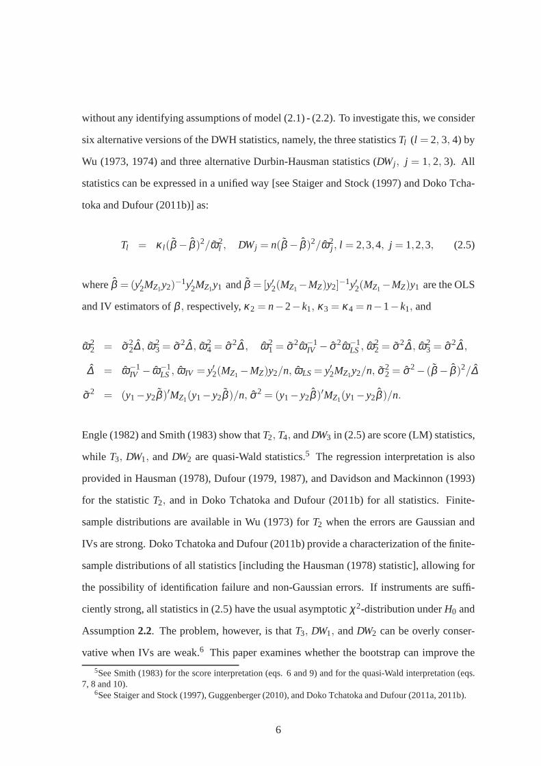
without any identifying assumptions of model (2.1) - (2.2).To investigate this, we consider

six alternative versions of the DWH statistics, namely, thethree statisticsTl (l = 2, 3, 4) by

Wu (1973, 1974) and three alternative Durbin-Hausman statistics (DWj , j = 1, 2, 3). All

statistics can be expressed in a unified way [see Staiger and Stock (1997) and Doko Tcha-

toka and Dufour (2011b)] as:

Tl = κ l(β − β )2/ω2l , DWj = n(β − β )2/ω2

j , l = 2,3,4, j = 1,2,3, (2.5)

whereβ = (y′2MZ1y2)−1y′2MZ1y1 andβ = [y′2(MZ1−MZ)y2]

−1y′2(MZ1−MZ)y1 are the OLS

and IV estimators ofβ , respectively,κ2 = n−2−k1, κ3 = κ4 = n−1−k1, and

ω22 = σ2

2∆ , ω23 = σ2∆ , ω2

4 = σ2∆ , ω21 = σ2ω−1

IV − σ2ω−1LS, ω2

2 = σ2∆ , ω23 = σ2∆ ,

∆ = ω−1IV − ω−1

LS, ω IV = y′2(MZ1 −MZ)y2/n, ωLS= y′2MZ1y2/n, σ22 = σ2− (β − β )2/∆

σ2 = (y1−y2β )′MZ1(y1−y2β )/n, σ2 = (y1−y2β )′MZ1(y1−y2β )/n.

Engle (1982) and Smith (1983) show thatT2, T4, andDW3 in (2.5) are score (LM) statistics,

while T3, DW1, andDW2 are quasi-Wald statistics.5 The regression interpretation is also

provided in Hausman (1978), Dufour (1979, 1987), and Davidson and Mackinnon (1993)

for the statisticT2, and in Doko Tchatoka and Dufour (2011b) for all statistics. Finite-

sample distributions are available in Wu (1973) forT2 when the errors are Gaussian and

IVs are strong. Doko Tchatoka and Dufour (2011b) provide a characterization of the finite-

sample distributions of all statistics [including the Hausman (1978) statistic], allowing for

the possibility of identification failure and non-Gaussianerrors. If instruments are suffi-

ciently strong, all statistics in (2.5) have the usual asymptotic χ2-distribution underH0 and

Assumption2.2. The problem, however, is thatT3, DW1, andDW2 can be overly conser-

vative when IVs are weak.6 This paper examines whether the bootstrap can improve the

5See Smith (1983) for the score interpretation (eqs. 6 and 9) and for the quasi-Wald interpretation (eqs.7, 8 and 10).

6See Staiger and Stock (1997), Guggenberger (2010), and DokoTchatoka and Dufour (2011a, 2011b).

6

size and power of the above DWH tests, especially when identification is not very strong.

Wong (1996) suggests that bootstrapping the Hausman (1978)exogeneity test improves

its size and power. Li (2006) extends this result to models with serially correlated errors.

However, neither Wong (1996) nor Li (2006) provides a formalproof of the validity of their

bootstraps even when IVs are strong. Both studies are Monte Carlo study experiments and

the designs of the experiments only consider cases where thestrength of the instruments is

moderate. In this paper, our analysis allows for any arbitrary level of instrument strength.

It is also worth noting that the exogeneity tests in (2.5) have their own shortcomings.

Indeed, Moreira (2009, footnote 1) shows that testingH0 : σv2u = 0 is equivalent to test

Hβ : β = β 0 in model (2.1)-(2.2), whereβ 0 = σ12/σ2v2, σ12= cov(v1t ,v2t), σ2

v2= var(v2t)

for all t = 1, . . . ,n, andv1 andv2 are given in (2.3). This means that doing a pre-test onσv2u

may imply important size distortions when making inferenceon β using a t-type test after

the pre-test. Guggenberger (2010) shows that the asymptotic size of the two-staget-test

where a DWH pre-test is used in the first-stage equals 1 for empirically relevant choices

of the parameter space. Despite this important issue, the DWH tests are still widely used

in many empirical work: for example, the Baum, Schaffer and Stillman (2003) versions of

these tests is now implemented in Stata and the study has morethan three hundred citations

in RePEc. Wong (1997) shows through a Monte Carlo study experiment that bootstrapping

substantially improves inference over the conventional pretesting procedure. Our goal in

this paper is to make progress in this direction.

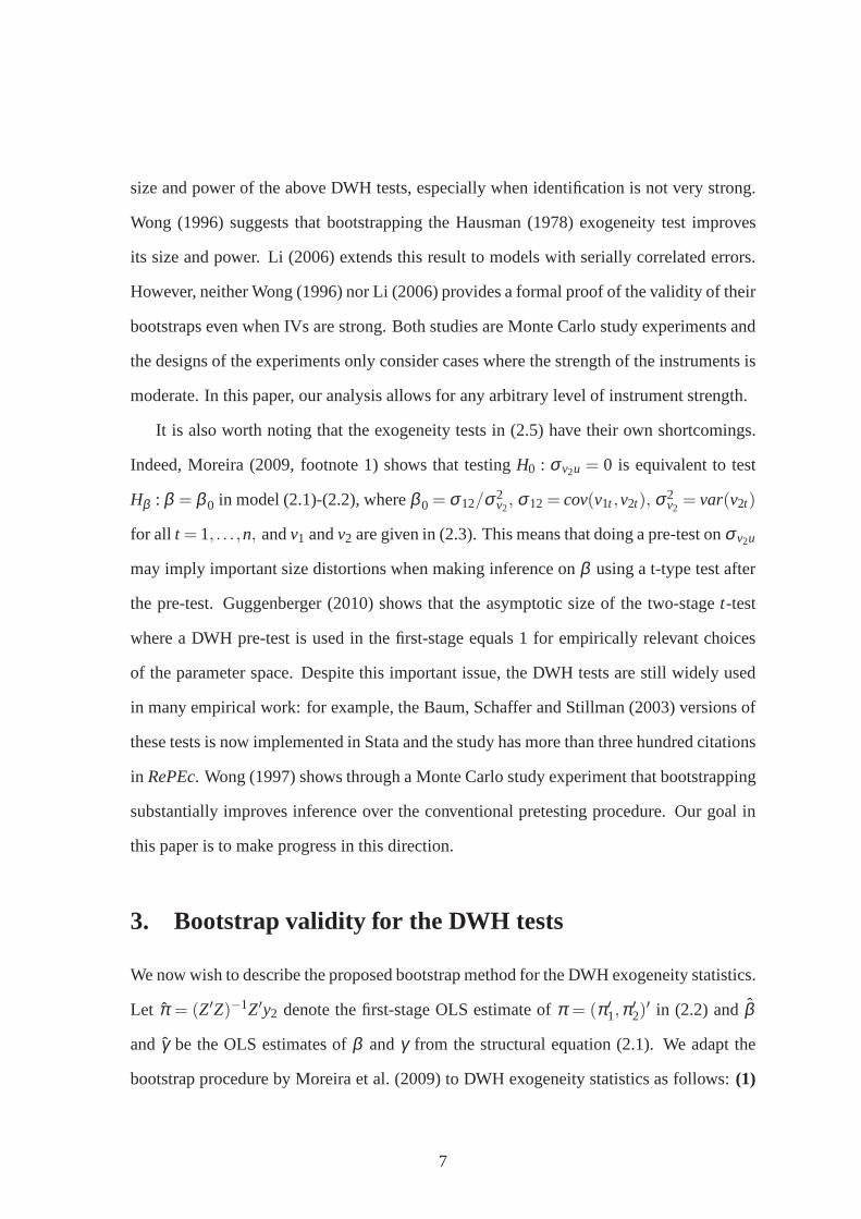
3. Bootstrap validity for the DWH tests

We now wish to describe the proposed bootstrap method for theDWH exogeneity statistics.

Let π = (Z′Z)−1Z′y2 denote the first-stage OLS estimate ofπ = (π ′1,π

′2)

′ in (2.2) andβ

and γ be the OLS estimates ofβ andγ from the structural equation (2.1). We adapt the

bootstrap procedure by Moreira et al. (2009) to DWH exogeneity statistics as follows:(1)

7

from the observed data, computeπ andβ along with all other things necessary to obtain

the realizations of the statisticsTl , DWj , and the residuals from the reduced-form equation

(2.3): v1 = y1−Z1(π1β + γ)−Z2π2β , v2 = y2−Zπ . These residuals are then re-centered

by subtracting sample means to yield(v1, v2); (2) for each bootstrap sampler = 1, . . . , B,

the data are generated following

y∗1 = Z∗1(π1β + γ)+Z∗

2π2β +v∗1, y∗2 = Z∗π +v∗2, (3.1)

whereZ∗ = [Z∗1 : Z∗

2] and (v∗1, v∗2) are drawn independently from the joint empirical dis-

tribution of Z and(v1, v2). The corresponding bootstrap statisticsT∗r

l andDW∗r

j are then

computed for each bootstrap sampler = 1, . . . , B; (3) the simulated bootstrapp-value of

each statistic is obtained as the proportion of bootstrap statistics that are more extreme than

the computed statistic from the observed data;(4) the corresponding bootstrap test rejects

exogeneity at levelα if its p-value is less thanα.

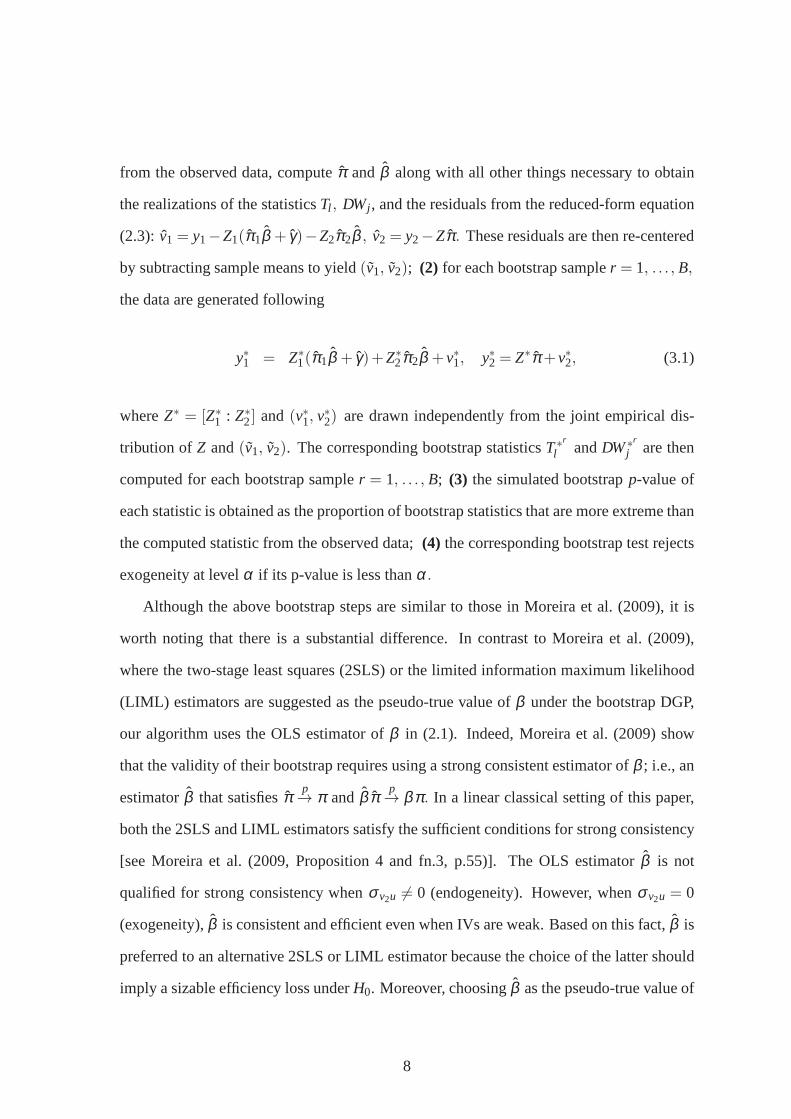
Although the above bootstrap steps are similar to those in Moreira et al. (2009), it is

worth noting that there is a substantial difference. In contrast to Moreira et al. (2009),

where the two-stage least squares (2SLS) or the limited information maximum likelihood

(LIML) estimators are suggested as the pseudo-true value ofβ under the bootstrap DGP,

our algorithm uses the OLS estimator ofβ in (2.1). Indeed, Moreira et al. (2009) show

that the validity of their bootstrap requires using a strongconsistent estimator ofβ ; i.e., an

estimatorβ that satisfiesπ p→ π andβ π p→ βπ. In a linear classical setting of this paper,

both the 2SLS and LIML estimators satisfy the sufficient conditions for strong consistency

[see Moreira et al. (2009, Proposition 4 and fn.3, p.55)]. The OLS estimatorβ is not

qualified for strong consistency whenσv2u 6= 0 (endogeneity). However, whenσv2u = 0

(exogeneity),β is consistent and efficient even when IVs are weak. Based on this fact,β is

preferred to an alternative 2SLS or LIML estimator because the choice of the latter should

imply a sizable efficiency loss underH0. Moreover, choosingβ as the pseudo-true value of

8

β whenH0 is false is suggested in Horowitz (1994, Section 2.3) to approximate the power

function of the bootstrap tests.7

In the reminder of the paper, letFn denote the empirical distribution ofR∗n =

vech(

(Y∗′n ,Z∗′

n )′(Y∗′

n ,Z∗′n )

)

conditional onFn = (Y′1, Z′

1), . . . , (Y′n, Z′

n) , P∗

be the proba-

bility under the empirical distribution function (conditional onFn), andE∗

its correspond-

ing expectation operator. Also, letG1(·) andg1(·) be the cumulative density function (cdf)

and the probability density function (pdf) of aχ2-distributed random variable with one de-

gree of freedom. In order to ease the exposition of our results, we shall deal separately with

the case where identification is strong and the one where it isweak. Since strong identifi-

cation is relatively easy to tackle, we will focus on that case first. Section 3.1 presents the

results.

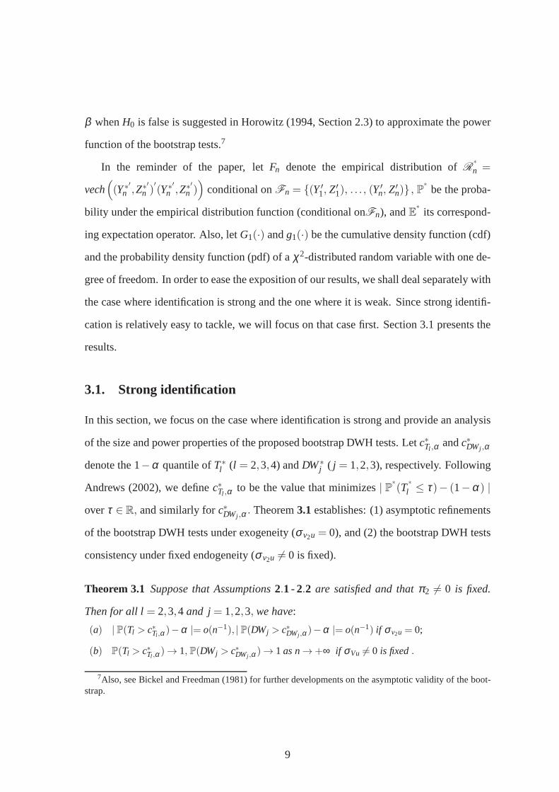
3.1. Strong identification

In this section, we focus on the case where identification is strong and provide an analysis

of the size and power properties of the proposed bootstrap DWH tests. Letc∗Tl ,α andc∗DWj ,α

denote the 1−α quantile ofT∗l (l = 2,3,4) andDW∗

j ( j = 1,2,3), respectively. Following

Andrews (2002), we definec∗Tl ,α to be the value that minimizes| P∗(T

∗l ≤ τ)− (1−α) |

overτ ∈ R, and similarly forc∗DWj ,α . Theorem3.1establishes: (1) asymptotic refinements

of the bootstrap DWH tests under exogeneity (σv2u = 0), and (2) the bootstrap DWH tests

consistency under fixed endogeneity (σv2u 6= 0 is fixed).

Theorem 3.1 Suppose that Assumptions2.1 - 2.2 are satisfied and thatπ2 6= 0 is fixed.

Then for all l= 2,3,4 and j= 1,2,3, we have:

(a) | P(Tl > c∗Tl ,α)−α |= o(n−1), | P(DWj > c∗DWj ,α)−α |= o(n−1) if σv2u = 0;

(b) P(Tl > c∗Tl ,α)→ 1, P(DWj > c∗DWj ,α)→ 1 as n→+∞ if σVu 6= 0 is fixed.

7Also, see Bickel and Freedman (1981) for further developments on the asymptotic validity of the boot-strap.

9

Theorem3.1-(a) gives the conditions under which the bootstrap critical values forT∗l

andDW∗j yield levels for theTl andDWj tests that are correct throughO(n−1) underH0. So,

the bootstrap makes an error of sizeO(n−1) under exogeneity, which is smaller asn→+∞

than bothO(n−1/2) and the error made by the first-order asymptotic approximations. The

bootstrap provides a greater accuracy than theO(n−1/2) order because all DWH statistics

are quadratic functions of symmetric pivotal statistics [see Horowitz (2001, Ch. 52, eq.

3.13)] under exogeneity (σv2u = 0) and strong identification (π2 6= 0). Theorem3.1-(b)

shows that test consistency holds if the bootstrap criticalvalues are used in the inference.

This is because the asymptotic distributions of all DWH statistics diverge under fixed en-

dogeneity (σv2u 6= 0 is fixed) and strong identification (π2 6= 0). Hence, test consistency

will still hold if the empiricalsize-correctedcritical values are used instead of the bootstrap

ones, as suggested by Horowitz (1994). Although Theorem3.1-(b) considers the case of

fixed endogeneity, there is no impediment to expanding it to local to zero alternatives of the

form H1c : σv2u = c/√

n for some scalarc 6= 0. In this case, test consistency does no longer

hold becauseσv2u → 0 asn→+∞ so that the limiting distributions of the bootstrap DWH

statistics are not far from their limiting distributions under exogeneity (σv2u = 0). How-

ever, we can provide high-order refinements of the power functions of the tests similar to

Theorem3.1-(a), where the Edgeworth expansion is run atµc = E(Rn) 6= 0; for example,

see Taniguchi (1988). This proof is omitted in order to shorten the exposition.

3.2. Local to zero weak instruments

We now analyze the Staiger and Stock (1997) local to zero weakinstruments framework.

To be more specific, we assume thatπ2 = π02/√

n, whereπ02 ∈ Rk2 is a fixed vector

(possibly zero). As argued previously, high-order refinements of the size of the tests in

Theorem3.1-(a) are no longer achievable due to identification failure.This is because the

functionsH(·) andH(·) in eqs.(A.2) - (A.3) of the appendix are no longer smooth around

µ =E(Rn). For example, both functions depend ony′2(MZ1−MZ)y2/n but their derivatives

10

with respect toy′2(MZ1 −MZ)y2/n is not well-defined whenπ2 = 0 or does not even exist

if π2 = π02cn for any sequencecn ↓ 0 [similar to Moreira et al. (2009, footnote 2)]. This is

particularly the case in the Staiger and Stock (1997) setup wherecn = 1/√

n. Nonetheless,

we can establish the following theorem on the first-order validity of the bootstrap.

Theorem 3.2 Suppose that Assumption2.2 is satisfied and thatπ2 = π02/√

n, where

π02 ∈ Rk2 is fixed. If further for someδ > 0, E(‖Zi‖4+δ , ‖vi‖2+δ )< ∞, then we have:

(a) | P(Tl > c∗Tl ,α)−α |= o(1), | P(DWj > c∗DWj ,α)−α |= o(1) if π02σv2u = 0;

(b) | P(Tl > c∗Tl ,α)− (1−αTl ) |= o(1), | P(DWj > c∗DWj ,α)− (1−αDWj ) |= o(1) if π02σVu 6= 0,

where αTl = E[G1(c∗Tl ,α ;‖µ‖2)] for l = 2,4, αT3 = E[(σ2u/σ2

u)G1(c∗T3,α ;‖µ‖2)], αDWj =

E[(σ2u/σ2

u)G1(c∗DWj ,α ;‖µ‖2)] for j = 1,2, αDW3 = E[G1(c∗DW3,α ;‖µ‖2)], G1(.;‖µ‖2) is the

cdf of a noncentralχ2 distributed random variable with one degree of freedom and non-centrality

parameter‖µ‖2, σ2u andµ are defined in LemmaA.4.

Theorem3.2-(a) holds in particular whenH0 : σv2u = 0 is satisfied. So, the bootstrap

critical values forT∗l andDW

∗j yield levels for theTl andDWj tests that are asymptotically

correct under exogeneity, despite the lack of identification. Since the statisticsT2, T4, and

DW3 are score statistics [see Engle (1982) and Smith (1983)], and that testingH0 is equiva-

lent to testHβ : β = β 0 = σ12/σ2v2

[see Moreira (2009, footnote 1)], the bootstrap validity

for these statistics under weak instruments is not surprising, as established in Moreira et al.

(2009). However, the bootstrap validity for the quasi-WaldtestsT3, DW1, andDW2 is not

intuitive. In general, the bootstrap often fails for Wald-type statistics when instruments are

weak because their limiting distributions often involve nuisance parameters; see Dufour

(1997, 2003, 2006), Andrews and Guggenberger (2010), and Moreira et al. (2009), among

others. The validity of the bootstrap for these statistics here is mainly justified by the fact

that they do not directly depend on the structural coefficient β even when endogeneity is

present; see Wu (1973, Section 3), Wu (1974, eqs. 3.11 - 3.16), and Doko Tchatoka and

Dufour (2011a, 2011b).

11

Theorem3.2-(b) indicates that the DWH tests may still exhibit power under weak in-

struments if the bootstrap critical values are used, provided thatπ02σv2u 6= 0. However,

the bootstrap critical values yield tests with power no higher than the nominal size for any

level of endogeneity ifπ02σv2u = 0, as showed Theorem3.2-(a). This is particularly the

case when all instruments are irrelevant (π02 = 0) so thatβ is completely unidentified.

This is because whenπ02σv2u = 0, the limiting distributions of all DWH statistics (both

the standard and bootstrap statistics) are the same as underexogeneity, despite the fact that

σv2u 6= 0; see LemmasA.4 andA.7 in Appendix. This result is intuitive becauseσv2u is

not identifiable ifβ is not identifiable [see Doko Tchatoka and Dufour (2014)], which is

the case8 whenπ02σv2u = 0. In many empirical applications, not all instruments are often

irrelevant, so, the bootstrap tests may have power if at least one instrument is not very poor.

4. Monte Carlo experiment

We use simulation to examine the finite-sample performance of the proposed bootstrap

DWH tests. The DGP is described by eqs. (2.1) and (2.2) withk1 = 0 [no exogenous

instruments in (2.1)],Z2 containsk2 = 5 instruments, each generatedi.i.d. N(0, 1) and

independent of(ut, v2t)′ for all t = 1, . . . , n. The true value ofβ is set at 2 and the

reduced-form coefficientπ2 is chosen asπ2 = λπ02, whereπ02 ∈ Rk2 is a vector of ones

and λ ∈ 0,0.05,0.1,1 characterizes the strength of the instruments.9 More precisely,

λ = 0 is a design of complete non-identification (irrelevant instruments),λ = 0.05 de-

signs weak identification,λ = 0.1 is the setup of moderate identification, and finallyλ = 1

symbolizes strong identification. The errors(ut , v2t)′ are generated as(ut, v2t)

′ = Jε t ,

whereε t ∼ N(0, I2) , J =

1ρv2u

(1+ρ2v2u)

1/2

0 1(1+ρ2

v2u)1/2

, andρv2u measures the endogeneity ofy2.

8Whenπ02σv2u = 0, all values of(β ,σ v2u) ∈R2 areobservationally equivalentso that the bootstrap tests

have no power to discriminate betweenσv2u 6= 0 andσv2u = 0.9Dufour and Taamouti (2007) and Doko Tchatoka (2014) consider similar data-generating processes for

the first-stage regression (2.2).

12

The exogeneity ofy2 is then expressed asH0 : ρv2u = 0. In this experiment, we varyρv2u

in −0.8,0,0.2,0.9, but the results do not change qualitatively for alternativevalues of

ρv2u. The rejection frequencies are computed using 1,000 replications for the standard

DWH tests, while those of the bootstrap tests are obtained with N = 1,000 replications and

B= 999 bootstrap pseudo-samples of sizen= 300.

Table 1 presents the results. In the first part of the table, the rejection frequencies of the

DWH tests are reported using both the bootstrap and usual asymptotic critical values. The

second part of the table reports the rejection frequencies of Wong’s (1997) second-stage

bootstrap tests as well as the usual second-stage two-sidedt-tests ofHβ : β = β 0 (after

pre-testing exogeneity). The nominal levels are set at 0.05 for both the pre-tests and the

second-stage tests. The first column of the table contains the statistics, while the others

present, for each value of the endogeneityρv2u and IV qualityλ , the empirical rejection

frequencies of the tests. The columnρv2u = 0 represents exogeneity, while those with

ρv2u 6= 0 indicate endogeneity.

First, we observe that the empirical rejection frequencies of allDWH tests when the

bootstrap critical values are used are close to the 5% nominal level whenρv2u= 0 (exogene-

ity), irrespective of the value ofλ (quality of the instruments), thus confirming our theoreti-

cal findings in Theorems3.1-(a) and Theorem3.2-(a). Meanwhile, only the LM versions of

these tests, namely,T2, T4, andDW3, have correct size asymptotically forλ ∈ 0,0.05,0.1

(weak or moderate instruments) when the usual asymptotic critical values are used in the

inference. The quasi-Wald versions of the DWH tests (T3, DW1, andDW2) are overly con-

servative under weak instruments [λ ∈ 0,0.05]. As expected, the rejection frequencies

of all tests are similar and close to the 5% nominal level under exogeneity (ρv2u = 0) and

strong identification (λ = 1), with both the bootstrap and asymptoticχ2 critical values.

Clearly, bootstrapping substantially improves the size ofT3, DW1, and DW2, especially

when identification is weak.

Second, whenρv2u 6= 0 (endogeneity), we observe that all tests have empirical rejec-

13

tions approaching or equal to 100% when identification is moderate or strong and endo-

geneity is large [see columnsρv2u ∈ −0.8,0.9 andλ ∈ 0.1,1], whether the bootstrap

or asymptoticχ2 critical values are used, thus confirming our theoretical findings in Theo-

rem3.1- (b). However, all tests have low power when identification is very weak [columns

ρv2u 6= 0 andλ ∈ 0,0.05] even if the bootstrap critical values are used, as expectedfrom

the theoretical results in Theorem3.2- (a). Nevertheless, even the quasi-Wald DWH tests

exhibit power with weak instruments and large endogeneity [see columnsλ = 0.05 and

ρv2u ∈ −0.8,0.9] if the bootstrap critical values are used, thus confirming the analysis in

Theorem3.2- (b). So, in contrast to the usual asymptoticχ2-critical values, the bootstrap

improves the power of the quasi-Wald versions of the DWH tests, provided that identifica-

tion is not completely irrelevant. For examples, the empirical rejection frequencies ofT3,

DW1, andDW2 with the bootstrap critical values whenρv2u = 0.9 andλ = 0.05 are around

24%. These represents nearly the triple of their rejection frequencies when the asymptotic

χ2-critical values are used (about 8%). Furthermore, the tests T3, DW1, andDW2 become

competitive with the bootstrap critical values in terms of power compared withT2, T4, and

DW3. Indeed, while the usual asymptotic LM tests (T2, T4, andDW3) strictly dominate the

quasi-Wald ones (T3, DW1, andDW2), the empirical rejection frequencies using the boot-

strap critical values are very close for all tests even when identification is not strong.

Finally, the second part of the table show that the size of theusual two-staget-tests,

where a DWH-type pre-test is used in the first-stage, is closeto 1 whenλ ∈ 0,0.05,0.1

(weak instruments) and endogeneity is present (ρv2u 6= 0).10 The usual two-staget-tests

have approximately good size asymptotically only when identification is very strongλ = 1

(see the bottom part of Table 1). In contrast, the bootstrap tests ofHβ : β = β 0, similar

to those of Wong (1997), substantially improves the size over the conventional two-stage

t-tests. For example, the maximal rejection frequencies of the proposed bootstrap tests

of Hβ : β = β 0 are around 12%, while those of the conventional two-staget-tests can

10Similar to Guggenberger (2010).

14

be as high as 99.9%. More interestingly, while the usual asymptotic LM versions of the

DWH tests (T2, T4, andDW3) have correct size and are (almost uniformly) more powerful

than their bootstrap’s counterparts, their use as pre-tests lead to serious size distortions

of the second staget-tests. Meanwhile, using the bootstrap versions of all DWH tests

(including the quasi-Wald DWH tests) substantially improves the conventional pre-testing

based-inference.

Acknowledgments

We are grateful to Professor Richard J. Smith, Managing Editor of The Econometrics Jour-

nal and two anonymous referees for their constructive commentsand suggestions. We

would also like to thank Professors Jean-Marie Dufour, Mardi Dungey, and Jan Kiviet for

several useful comments. This project is supported by a Faculty of Business and School of

Economics and Finance (University of Tasmania) jointresearch grant, and I am grateful

for their support.

APPENDIX

A. Auxiliary Lemmata and Proofs

In the remainder of this appendix, we defineSl ,n =√

n(β − β )/ω l and Sj,n =√

n(β − β )/ω j ,

l = 2,3,4; j = 1,2,3, whereβ , β , ω l , and ω j are given in (2.5). It is then easy to see that the

statisticsTl (l = 2,3,4) andDWj ( j = 1,2,3) in (2.5) can be expressed as

Tl = n−1κ l ‖ Sl ,n ‖2, DWj =‖ Sj,n ‖2 . (A.1)

We shall now state the following auxiliary lemmas that are used in the proofs of the main results.

15

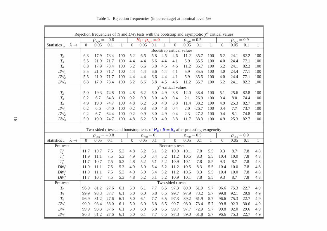
Table 1. Rejection frequencies (in percentage) at nominal level 5%

Rejection frequencies ofTl andDWj tests with the bootstrap and asymptoticχ2 critical valuesρv2u =−0.8 H0 : ρv2u = 0 ρv2u = 0.5 ρv2u = 0.9

Statistics↓ λ → 0 0.05 0.1 1 0 0.05 0.1 1 0 0.05 0.1 1 0 0.05 0.1 1Bootstrap critical values

T2 6.8 17.9 73.4 100 5.2 6.6 5.8 4.5 4.6 11.2 35.7 100 6.2 24.1 82.2100T3 5.5 21.0 71.7 100 4.4 4.4 6.6 4.4 4.1 5.9 35.5 100 4.0 24.4 77.1 100T4 6.8 17.9 73.4 100 5.2 6.6 5.8 4.5 4.6 11.2 35.7 100 6.2 24.1 82.2100

DW1 5.5 21.0 71.7 100 4.4 4.4 6.6 4.4 4.1 5.9 35.5 100 4.0 24.4 77.1 100DW2 5.5 21.0 71.7 100 4.4 4.4 6.6 4.4 4.1 5.9 35.5 100 4.0 24.4 77.1 100DW3 6.8 17.9 73.4 100 5.2 6.6 5.8 4.5 4.6 11.2 35.7 100 6.2 24.1 82.2100

χ2-critical valuesT2 5.0 19.3 74.8 100 4.8 6.2 6.0 4.9 3.8 12.0 38.4 100 5.1 25.6 82.8100T3 0.2 6.7 64.3 100 0.2 0.9 3.0 4.9 0.4 2.1 26.9 100 0.4 8.0 74.4 100T4 4.9 19.0 74.7 100 4.8 6.2 5.9 4.9 3.8 11.4 38.2 100 4.9 25.3 82.7100

DW1 0.2 6.6 64.0 100 0.2 0.8 3.0 4.8 0.4 2.0 26.7 100 0.4 7.7 73.7 100DW2 0.2 6.7 64.4 100 0.2 0.9 3.0 4.9 0.4 2.3 27.2 100 0.4 8.1 74.8 100DW3 5.0 19.0 74.7 100 4.8 6.2 5.9 4.9 3.8 11.7 38.3 100 4.9 25.3 82.7100

Two-sidedt-tests and bootstrap tests ofHβ : β = β 0 after pretesting exogeneityρv2u =−0.8 ρv2u = 0 ρv2u = 0.5 ρv2u = 0.9

Statistics↓ λ → 0 0.05 0.1 1 0 0.05 0.1 1 0 0.05 0.1 1 0 0.05 0.1 1Pre-tests Bootstrap tests

T∗2 11.7 10.7 7.5 5.3 4.8 5.2 5.1 5.2 10.9 10.1 7.8 5.5 9.3 8.7 7.8 4.8

T∗3 11.9 11.1 7.5 5.3 4.9 5.0 5.4 5.2 11.2 10.5 8.3 5.5 10.4 10.0 7.84.8

T∗4 11.7 10.7 7.5 5.3 4.8 5.2 5.1 5.2 10.9 10.1 7.8 5.5 9.3 8.7 7.8 4.8

DW∗1 11.9 11.1 7.5 5.3 4.9 5.0 5.4 5.2 11.2 10.5 8.3 5.5 10.4 10.0 7.84.8

DW∗2 11.9 11.1 7.5 5.3 4.9 5.0 5.4 5.2 11.2 10.5 8.3 5.5 10.4 10.0 7.84.8

DW∗3 11.7 10.7 7.5 5.3 4.8 5.2 5.1 5.2 10.9 10.1 7.8 5.5 9.3 8.7 7.8 4.8

Pre-tests Two-sidedt-testsT2 96.9 81.2 27.6 6.1 5.0 6.1 7.7 6.5 97.3 89.0 61.9 5.7 96.6 75.3 22.7 4.9T3 99.9 93.3 37.7 6.1 5.0 6.0 6.8 6.5 99.7 97.9 73.2 5.7 99.8 92.1 29.9 4.9T4 96.9 81.2 27.6 6.1 5.0 6.1 7.7 6.5 97.3 89.2 61.9 5.7 96.6 75.3 22.7 4.9

DW1 99.9 93.4 38.0 6.1 5.0 6.0 6.8 6.5 99.7 98.0 73.4 5.7 99.8 92.3 30.6 4.9DW1 99.9 93.3 37.6 6.1 5.0 6.0 6.8 6.5 99.7 97.7 72.9 5.7 99.8 92.0 29.6 4.9DW1 96.8 81.2 27.6 6.1 5.0 6.1 7.7 6.5 97.3 89.0 61.8 5.7 96.6 75.3 22.7 4.9

16

A.1. Auxiliary Lemmata

Lemma A.1 Suppose that Assumptions2.1 - 2.2 are satisfied and thatπ2 6= 0 is fixed. Then we

have:

(a) supτ ∈R | P(Sl ,n ≤ τ)−Φ(τ)−∑s−2h=1 n

−h/2ph

Sl ,n(τ ;F,π2)φ (τ) |= o(n

− s−22 ),

supτ ∈R | P(Sj,n ≤ τ)−Φ(τ)−∑s−2h=1n

−h/2ph

Sj,n(τ ;F,π2)φ (τ) |= o(n

− s−22 ) if σ v2u = 0;

(b) supτ ∈RP(|Sl ,n| ≤ τ)→ 0, supτ ∈RP(|Sj,n| ≤ τ)→ 0 as n→+∞ if σVu 6= 0 is fixed,

whereΦ(·) andφ(·) are the cdf and pdf of a standard normal random variable, phSl ,n

and

phSj,n

are polynomials inτ with coefficients depending onβ , π2, and the moments of the

distribution F ofRn.

Lemma A.2 Suppose that Assumptions2.1 - 2.2 are satisfied and thatπ2 6= 0 is fixed. Then for

some r∈ N, we have:

(a) supτ ∈R | P(Tl ≤ τ)−G1(τ)−∑rh=1n

−hph

Tl ,n(τ ;F,π2)g1(τ) |= o(n−r ),

supτ ∈R | P(DWj ≤ τ)−G1(τ)−∑rh=1n

−hph

DWj,n(τ ;F,π2)g1(τ) |= o(n−r) if σ v2u = 0;

(b) supτ ∈RP(Tl ≤ τ)→ 0, supτ ∈RP(DWj ≤ τ)→ 0 as n→+∞ if σVu 6= 0 is fixed,

where G1(·) and g1(·) are the cdf and pdf of aχ2(1)-distributed random variable, phTl ,n

and phDWj,n

are polynomials inτ with coefficients depending onβ , π2, and the moments of

the distribution F ofRn.

Lemma A.3 Suppose that Assumptions2.1 - 2.2 are satisfied and thatπ2 6= 0 is fixed. Then for

some r∈ N, we have:

(a) supτ ∈R | P∗(T∗l ≤ τ)−G1(τ)−∑r

h=1n−h

phTl(τ ;Fn, β , π2)g1(τ) |= o(n−r),

supτ ∈R | P∗(DW∗j ≤ τ)−G1(τ)−∑r

h=1n−h

phDWj

(τ ;Fn, β , π2)g1(τ) |= o(n−r) a.s. if σ v2u = 0;

(b) supτ ∈RP∗(T

∗l ≤ τ)→ 0, supτ ∈RP

∗(DW∗j ≤ τ)→ 0 a.s. as n→+∞ if σVu 6= 0 is fixed,

phTl, ph

DWjare polynomials inτ with coefficients depending onβ , π2 and the moments of Fn.

Lemma A.4 Suppose Assumption2.2 is satisfied and thatπ2 = π02/√

n, π02 ∈ Rk2 is fixed. Then

we have:

(a) T2,T4,H3d→ χ2(1)and T3,H1,H2 | ψZ2v2

d→ σ2u

σ2uχ2(1)≤ χ2(1) whenπ02σv2u = 0;

(b) T2,T4,H3 | ψZ2v2

d→ χ2(1,‖µ‖2) and T3,H1,H2d→ σ2

uσ2

uχ2(1,‖µ‖2)≤ χ2(1,‖µ‖2)

whenπ02σ v2u 6= 0, whereµ = σ−1u σ−2

v2Ψ−1/2

Z2v2Q−1

Z2π02σv2u

17

with ΨZ2v2 = (ψZ2v2+ QZ2π02)

′Q−1Z2(ψZ2v2

+ QZ2π02), ψZ2v2= ψZ2v2

− QZ2Z1Q−1Z1

ψZ1v2, ψZ2u =

ψZ2u − QZ2Z1Q−1Z1

ψZ1u, σ2u = σ2

u − 2σ v2uΨ−1Z2v2

(ψZ2v2+ QZ2π02)

′Q−1Z2

ψZ2u + σv2ψ ′Z2uQ−1

Z2(ψZ2v2

+

QZ2π02)Ψ−2Z2v2

(ψZ2v2+ QZ2π02)

′Q−1Z2

ψZ2u, andQZ2 = QZ2 −QZ2Z1Q−1Z1

Q′Z2Z1

.

LemmaA.4-(a) holds in particular whenσ v2u = 0 (exogeneity). So,T2, T4 andH3 are pivotal

under weak instruments and exogeneity, whileH1, H2 andT3 are boundly pivotal. Since Lemma

A.4-(a) may still hold even ifσ v2u 6= 0, hence all exogeneity tests have no power against endogeneity

if π02σ v2u = 0. This is the case ifπ02 = 0 (irrelevant IVs) so that (a) holds for any value ofσ v2u:

the power of all tests cannot exceed the nominal level asymptotical; see Doko Tchatoka and Dufour

(2011b). However, all tests exhibit power against endogeneity even when IVs are weak, provided

thatπ02σ v2u 6= 0, as showed LemmaA.4-(b).

Lemma A.5 Suppose that Assumption2.2 is satisfied and that H0 holds. If for someδ > 0, we

haveE(‖Zt‖2+δ , ‖vt‖2+δ ) < ∞, thenE∗(|Z∗

jt v∗mt|2+δ ) andE

∗(|Z∗

ji u∗i |2+δ ) are bounded a.s. for all

j = 1, . . . ,k and m= 1, 2; where Z∗ and v∗ = [v∗1 : v∗2] are the bootstrap draws from the empirical

distribution of Z and the re-centered residualsv= [v1 : v2], and u∗ = v∗1−v∗2β .

Lemma A.6 Suppose that Assumption2.2 is satisfied. If for some δ > 0,

E(‖Zi‖4+δ , ‖vi‖2+δ ) < ∞, then under H0, we have 1√n

(

Z∗u∗,Z∗v∗2,(W∗′

1

n − W′1

n ))

| Fnd→

N

0,

diag(σ 2u, σv2)⊗QZ 0

0 Σw

a.s, where W = (w1, . . . , wn), wi = vech(ZiZ′

i ),

W∗ = (w∗1, . . . , w∗

n), w∗i = vech(Z∗

i Z∗′i ) ∈ R

k(k+1)/2, Σw = var(wi), and 1 is a (n by 1) con-

stant vector of ones.

Lemma A.7 Suppose Assumption2.2 is satisfied and letπ2 = π02/√

n, π02 ∈ Rk2 is fixed. If for

someδ > 0, E(‖Zi‖4+δ , ‖vi‖2+δ )< ∞, then, conditional onFn, we have:

(a) T∗2 ,T

∗4 ,H

∗3

d→ χ2(1) and T∗3 ,H∗1 ,H

∗2 | ψZ2v2

d→ σ2u

σ2uχ2(1)≤ χ2(1)a.s.whenπ02σv2u = 0;

(b) T∗2 ,T

∗4 ,H

∗3 | ψZ2v2

d→ χ2(1,‖µ‖2) and T∗3 ,H∗1 ,H

∗2 | ψZ2v2

d→ σ2u

σ2uχ2(1,‖µ‖2)≤ χ2(1,‖µ‖2)

a.s. whenπ02σ v2u 6= 0.

Lemma A.8 Suppose Assumption2.2 is satisfied and letπ2 = π02/√

n, whereπ02∈Rk2 is fixed. If

for someδ > 0, E(‖Zi‖4+δ , ‖vi‖2+δ )< ∞, then we have: supτ ∈R | P∗(T∗l ≤ τ)−P(Tl ≤ τ) |= op(1)

18

and supτ ∈R | P∗(DW∗j ≤ τ)−P(DWj ≤ τ) |= op(1) for any value ofσ v2u.

A.2. Proofs

PROOF OFLEMMA A.1 (a) Suppose first thatH0 is satisfied (i.e.,σv2u = 0). We can expressSl ,n

andSj,n as:

Sl ,n =(1)√

n(y′2MZ1y2/n)−1(y′2MZ1y1/n)− (y′2(MZ1 −MZ)y2/n)−1(y′2(MZ1 −MZ)y1/n)

√

y′1My2 y1n [(

y′2(MZ1−MZ)y2n )−1− (

y′2MZ1y2n )−1]− [(

y′2MZ1 y2n )−1(

y′2MZ1y1n )− (

y′2(MZ1−MZ)y2n )−1(

y′2(MZ1−MZ)y1n )]2

=(2)√

n(y′2MZ1y2/n)−1(y′2MZ1u/n)− (y′2(MZ1 −MZ)y2/n)−1(y′2(MZ1 −MZ)u/n)

√

y′1My2 y1n [(

y′2(MZ1−MZ)y2n )−1− (

y′2MZ1y2n )−1]− [(

y′2MZ1 y2n )−1(

y′2MZ1y1n )− (

y′2(MZ1−MZ)y2n )−1(

y′2(MZ1−MZ)y1n )]2

=(3)√

nH(Rn) =√

n[

H(Rn)−H(µ)]

(A.2)

Sj,n =(1)√

n(y′2MZ1y2/n)−1(y′2MZ1y1/n)− (y′2(MZ1 −MZ)y2/n)−1(y′2(MZ1 −MZ)y1/n)

√

y′1My2 y1n [(

y′2(MZ1−MZ)y2n )−1− (

y′2MZ1y2n )−1]

=(2)√

n(y′2MZ1y2/n)−1(y′2MZ1u/n)− (y′2(MZ1 −MZ)y2/n)−1(y′2(MZ1 −MZ)u/n)

√

y′1My2 y1n [(

y′2(MZ1−MZ)y2n )−1− (

y′2MZ1 y2n )−1]

=(3)√

nH(Rn) =√

n[H(Rn)− H(µ)] (A.3)

where H(y2y2, y2y1, y2y2, y2y1, y1y1) =(y′2y2)

−1y′2y1−(y′2y2)−1y′2y1√

y′1y1[(y′2y2)−1−(y′2y2)−1]−[(y′2y2)−1y′2y1−(y′2y2)−1y′2y1]and

H(y2y2, y2y1, y2y2, y2y1, y1y1) =(y′2y2)

−1y′2y1−(y′2y2)−1y′2y1√

y′1y1[(y′2y2)−1−(y′2y2)−1]are real-valued Borel measurable func-

tions onRm with derivatives of orders≥ 3 and lower, being continuous on the neighborhood of

µ = E(Rn) whenπ2 6= 0 is fixed,H(µ) = 0 andH(µ) = 0 underH0. Note that the derivatives of

orders≥ 3 and lower ofH(·) andH(·) with respect toy′2MZ1y2/n, y′2MZ1y1/n, y′2(MZ1 −MZ)y1/n,

and y′1My2y1/n are well define for any value ofπ2. However, their derivatives with respect to

y′2(MZ1 −MZ)y2/n is not well-defined whenπ2 = 0 and does not even exist ifπ2 = π02cn for any

sequencecn ↓ 0 [similar to Moreira et al. (2009, footnote 2)]. The resultsin LemmaA.1 - (a) follow

from (A.2)-(A.2) by using Bhattacharya and Ghosh (1978, Theorem 2).

(b) Suppose now thatσv2u 6= 0 is fixed. Since π2 6= 0 is fixed and As-

sumption 2.2 holds, we can writeSl ,n =√

n(n−1/2Sl ,n − µ l ,S) +√

nµ l ,S, where µ l ,S =

plimn→+∞ n−1/2Sl ,n = − 1σu[π ′

2(QZ2 − Q′Z1Z2

Q−1Z1

QZ1Z2)π2 + σ v2]−1σv2u 6= 0 and

√n(n−1/2Sl ,n −

µ l ,S)d→ ψ l ,S ∼ N

0, [π ′2(QZ2 −Q′

Z1Z2Q−1

Z1QZ1Z2)π2]

−1− [π ′2(QZ2 −Q′

Z1Z2Q−1

Z1QZ1Z2)π2+σv2]

−1

,

and similarly for Sj,n. Therefore, for any τ ∈ R, we have limn→+∞P(|Sl ,n| ≤ τ) =

limn→+∞P(|√n(n−1/2Sl ,n−µ l ,S)+√

nµ l ,S| ≤ τ)≤ limn→+∞P(|√n(n−1/2Sl ,n−µ l ,S)|+√

n|µ l ,S| ≤

τ) → P(|ψ l ,S|+∞ ≤ τ) = 0, and similarly we have limn→+∞P(|Sj,n| ≤ τ) → 0. It immediately

19

follows that supτ ∈R | P(|Sl ,n| ≤ τ) |→ 0 and supτ ∈R | P(|Sj,n| ≤ τ) |→ 0, as stated.

PROOF OFLEMMA A.2 (a) Suppose first thatH0 is satisfied. Since we haveTl = n−1κ l ‖ Sl ,n ‖2

andDWj =‖ Sj,n ‖2 from (A.1) for all l and j, it suffices to approximateP(Tl ≤ τ) andP(DWj ≤ τ)

uniformly in τ to complete the proof. First, we can write bothP(Tl ≤ τ) andP(DWj ≤ τ) as:

P(Tl ≤ τ) = P(Sl ,n ∈ Cτ), P(DWj ≤ τ) = P(Sj,n ∈ Cτ), (A.4)

whereCτ =

x∈ R;x2 ≤ τ

are convex sets. From Bhattacharya and Rao (1976, Corollary3.2), we

have supτ∈R Φ((∂Cτ)ε) ≤ d.ε for some constantd andε > 0. So, Bhattacharya and Ghosh (1978,

Theorem 1) holds withB= Cτ andWn ∈ Sl ,n, Sj,n. By using the approximation ofP(Sl ,n ≤ τ) and

P(Sj,n ≤ τ) in LemmaA.1 - (a) and the definition ofCτ in (A.4), LemmaA.2 - (a) follows directly

from the fact that the odd terms of the quadratic expansion are even [see also Horowitz (2001, Ch.52,

eq.3.13) for the high-order approximation of pivotal symmetric statistics].

PROOF OFLEMMA A.3 The proof of (a) follows the same steps as Theorem 3 of Moreiraet al.

(2009) and is therefore omitted. The proof of (b) follows similar steps to those of LemmaA.1 - (b),

thus it is also omitted.

PROOF OF THEOREM 3.1 The proof of Theorem3.1-(a) is similar Hall and Horowitz (1996)

by exploiting LemmasA.2-A.3, hence is therefore omitted. Note that LemmasA.3-(a) shows that

the bootstrap estimates and the(r +1)-term empirical Edgeworth expansion in LemmaA.2-(a) for

all statistics are asymptotically equivalent up to theo(n−r) order underH0. Theorem3.1-(b) holds

mainly because the asymptotic distributions of all DWH statistics diverge under fixed endogeneity

(σ v2u 6= 0 is fixed) and strong identification (π 6= 0); as showed LemmaA.2-(b).

PROOF OFLEMMA A.4 LemmaA.4 is a special case of Doko Tchatoka and Dufour (2011a) for

G= 1, therefore the proof is omitted.

20

PROOF OFLEMMA A.5 The proof of LemmaA.5 is similar to those of Lemma A.1 in Moreira

et al. (2009) and is therefore omitted.

PROOF OFLEMMA A.6 The proof of LemmaA.6 is similar to those of Lemma A.2 in Moreira

et al. (2009) and is also omitted.

PROOF OFLEMMA A.7 First, we can write the bootstrap DWH statistics as

T∗l = n−1κ l ‖ S∗l ,n ‖2, DW∗

j =‖ S∗j,n ‖2, (A.5)

where S∗l ,n =√

n(β ∗ − β∗)/ω∗

l and S∗j,n =√

n(β ∗ − β∗)/ω∗

j , and β ∗, β

∗, ω∗

l , ω∗j are the boot-

strap counterparts ofβ , β , ω l , and ω j , respectively. Now, observe thatE∗(Z∗′Z∗/n) = Z′Z/n,

E∗(Z∗′u∗/n) = Z′u/n, E

∗(Z∗′v∗2/n) = Z′v2/n, andE

∗[(u∗ : v∗2)

′(u∗ : v∗2)/n] = (u : v2)′(u : v2)/n.

So, conditional onFn, we have by the Markov law of large numbers:Z∗′Z∗/n− Z′Z/n → 0,

Z∗′u∗/n− Z′u/n → 0, Z∗′v∗2/n− Z′v2/n → 0, and (u∗ : v∗2)′(u∗ : v∗2)/n− (u : v2)

′(u : v2)/n →

0 a.s. Since Z′Z/np→ QZ, Z′v2/n

p→ 0, Z′u/np→ 0, and (u : v2)

′(u : v2)/np→ Σ , hence we

have Z∗′Z∗/n → QZ, Z∗′u∗/n → 0, Z∗′v∗2/n → 0, and (u∗ : v∗2)′(u∗ : v∗2)/n → Σ a.s. under As-

sumption 2.2. Now, if π2 = π02/√

n and LemmaA.6 holds, we can show that (condi-

tional onFn): S∗2,n, S∗4,n, S∗3,nd→ Ψβ = 1

σuΨ−1/2

Z2v2(ψZ2v2

+ QZ2π02)′Q−1

Z2ψZ2u − 1

σuΨ 1/2

Z2v2σ−2

v2σ v2u and

S∗3,n, S∗1,n, S∗2,nd→ (σu/σu)Ψβ a.s., whereΨZ2v2 = (ψZ2v2

+QZ2π02)′Q−1

Z2(ψZ2v2

+QZ2π02), ψZ2v2=

ψZ2v2− QZ2Z1Q

−1Z1

ψZ1v2∼ N(0, σ2

v2QZ2), ψZ2u = ψZ2u − QZ2Z1Q

−1Z1

ψZ1u ∼ N(0, σ2uQZ2), QZ2 =

QZ2−QZ2Z1Q−1Z1

Q′Z2Z1

, andσ2u = σ2

u−2σv2uΨ−1Z2v2

(ψZ2v2+QZ2π02)

′Q−1Z2

ψZ2u+σv2ψ ′Z2uQ−1

Z2(ψZ2v2

+

QZ2π02)Ψ−2Z2v2

(ψZ2v2+ QZ2π02)

′Q−1Z2

ψZ2u. Moreover, we haveΨβ | ψZ2v2

d→ N(µ , 1), where µ =

σ−1u Ψ−1/2

Z2v2Q−1

Z2π02σ−2

v2σv2u = σ−1

u σ−2v2

Ψ−1/2Z2v2

Q−1Z2

π02σ v2u. We will now distinguish the following

two cases: (a)π02σ v2u = 0 and (b)π02σ v2u 6= 0.

(a) Suppose first thatπ02σv2u = 0. Then, we haveµ = 0 so thatΨβ | ψZ2v2

d→ N(0, 1). As a

result, we also haveT∗2 ,T

∗4 ,H

∗3 | ψZ2v2

d→ χ2(1) andT∗3 ,H

∗1 ,H

∗2 | ψZ2v2

d→ Ψ0 =σ2

uσ2

uχ2(1) ≤ χ2(1)

from (A.5). Hence, LemmaA.7-(a) follows immediately.

21

(b) Suppose now thatπ02σv2u 6= 0. Then, we haveµ 6= 0 so thatT∗2 ,T

∗4 ,H

∗3 | ψZ2v2

d→

χ2(1,‖µ‖2), T∗3 ,H

∗1 ,H

∗2 | ψZ2v2

d→ σ2u

σ2uχ2(1,‖µ‖2)≤ χ2(1,‖µ‖2), and LemmaA.7-(b) follows.

PROOF OFLEMMA A.8 LemmaA.8 follows directly from LemmasA.4-A.7.

PROOF OFTHEOREM 3.2 From LemmaA.8, we haveP(Tl > τ)−P∗(T∗

l > τ) = op(1) uniformly

overτ ∈ R. So, the results follow from LemmaA.7 and an expected value argument.

References

Andrews, D. W., Guggenberger, P. , 2010. Asymptotic size anda problem with subsampling and

with them out ofn bootstrap. Econometric Theory 26(2), 426–468.

Andrews, D. W. K., 2002. High-order improvement of a computationally attractive k-step bootstrap

for extremum estimators. Econometrica 70(1), 119–162.

Andrews, D. W. K., Stock, J. H., 2007. Inference with weak instruments. In: R. Blundell, W. Newey

, T. Pearson, eds, Advances in Economics and Econometrics, Theory and Applications, 9th

Congress of the Econometric Society Vol. 3. Cambridge University Press, Cambridge, U.K.,

chapter 6.

Baum, C., Schaffer, M. , Stillman, S. , 2003. Instrumental variables and GMM: Estimation and

testing. Stata Journal 3(1), 1–30.

Bhattacharya, R. N. , Ghosh, J. , 1978. On the validity of the formal Edgeworth expansion. The

Annals of Statistics 6, 434–451.

Bhattacharya, R. N., Rao, R., 1976. Normal approximation and asymptotic expansions. In: R. Bhat-

tacharya, R. Rao, eds, Normal Approximation and AsymptoticExpansions. Wiley Series in

Probability and Mathematical Analysis, New York.

22

Bickel, P. J. , Freedman, D. A. , 1981. Some asymptotic theoryfor the bootstrap. The Annals of

Statistics 9(6), 1196–1217.

Davidson, R., Mackinnon, J., 1993. Econometric Theory and Methods. Oxford University Press,

New York, New York.

Doko Tchatoka, F., 2014. Subset hypotheses testing and instrument exclusion in the linear IV re-

gression. Econometric Theory forthcoming.

Doko Tchatoka, F., Dufour, J.-M., 2011a. Exogeneity tests and estimation in IV regressions. Tech-

nical report, Department of Economics, McGill University Montreal, Canada.

Doko Tchatoka, F., Dufour, J.-M., 2011b. On the finite-sample theory of exogeneity tests with possi-

bly non-Gaussian errors and weak identification. Technicalreport, Department of Economics,

McGill University Montreal, Canada.

Doko Tchatoka, F., Dufour, J.-M., 2014. Identification-robust inference for endogeneity parameters

in linear structural models. The Econometrics Journal 17, 165–187.

Dufour, J.-M., 1979. Methods for Specification Errors Analysis with Macroeconomic Applications

PhD thesis University of Chicago. 257 + XIV pages.

Dufour, J.-M., 1987. Linear Wald methods for inference on covariances and weak exogeneity tests

in structural equations. In: I. B. MacNeill , G. J. Umphrey, eds, Advances in the Statistical

Sciences: Festschrift in Honour of Professor V.M. Joshi’s 70th Birthday. Volume III, Time

Series and Econometric Modelling. D. Reidel, Dordrecht, The Netherlands, pp. 317–338.

Dufour, J.-M., 1997. Some impossibility theorems in econometrics, with applications to structural

and dynamic models. Econometrica 65, 1365–1389.

Dufour, J.-M. , 2003. Identification, weak instruments and statistical inference in econometrics.

Canadian Journal of Economics 36(4), 767–808.

Dufour, J.-M. , 2006. Monte Carlo tests with nuisance parameters: A general approach to finite-

sample inference and nonstandard asymptotics in econometrics. Journal of Econometrics

138, 2649–2661.

23

Dufour, J.-M., Taamouti, M., 2007. Further results on projection-based inference in IV regressions

with weak, collinear or missing instruments. Journal of Econometrics 139(1), 133–153.

Durbin, J., 1954. Errors in variables. Review of the International Statistical Institute 22, 23–32.

Engle, R. F., 1982. A general approach to Lagrange multiplier diagnostics. Journal of Econometrics

20, 83–104.

Farebrother, R. W., 1976. A remark on the Wu test. Econometrica 44, 475–477.

Guggenberger, P., 2010. The impact of a Hausman pretest on the size of the hypothesis tests. Econo-

metric Theory 156, 337–343.

Hahn, J., Ham, J., Moon, H. R., 2010. The Hausman test and weakinstruments. Journal of Econo-

metrics 160, 289–299.

Hall, P., Horowitz, J. L., 1996. Bootstrap critical values for tests based on generalized-method-of-

moments estimators. Econometrica 64(4), 891–916.

Hausman, J., 1978. Specification tests in econometrics. Econometrica 46, 1251–1272.

Holly, A., 1982. A remark on Hausman’s test. Econometrica 50, 749–759.

Horowitz, J. L. , 1994. Bootstrap-based critical values forthe IM test. Journal of Econometrics

61, 395–411.

Horowitz, J. L., 2001. The bootstrap. In: J. Heckman, E. E. Leamer, eds, Handbook of Econometrics.

Elsvier Science, Amsterdam, The Netherlands.

Hwang, H.-S. , 1980. Test of independence between a subset ofstochastic regressors and distur-

bances. International Economic Review 21, 749–760.

Hwang, H.-S., 1985. The equivalence of Hausman and Lagrangemultiplier tests of independence

between disturbance and a subset of stochastic regressors.Economics Letters 17, 83–86.

Kariya, T., Hodoshima, H., 1980. Finite-sample propertiesof the tests for independence in structural

systems and LRT. The Quarterly Journal of Economics 31, 45–56.

24

Kiviet, J. F., Niemczyk, J., 2007. The asymptotic and finite-sample distributions of OLS and simple

IV in simultaneous equations. Computational Statistics and Data Analysis 51, 3296–3318.

Kiviet, J. F., Niemczyk, J., 2012. Comparing the asymptoticand empirical (un)conditional distri-

butions of OLS and IV in a linear static simultaneous equation. Computational Statistics and

Data Analysis 56, 3567–3586.

Kiviet, J. F., Pleus, M., 2012. The performance of tests on endogeneity of subsets of explanatory

variables scanned by simulation. Technical report, Amsterdam School of Economics Amster-

dam, The Netherlands.

Li, J., 2006. The block bootstrap test of Hausman’s exogeneity in the presence of serial correlation.

Economics Letters 91, 76–82.

Moreira, M. J., 2009. Tests with correct size when instruments can be abitrarily weak. Journal of

Econometrics 152, 131–140.

Moreira, M. J., Porter, J., Suarez, G., 2009. Bootstrap validity for the score test when instruments

may be weak. Journal of Econometrics 149, 52–64.

Nakamura, A., Nakamura, M., 1981. On the relationships among several specification error tests

presented by Durbin, Wu and Hausman. Econometrica 49, 1583–1588.

Revankar, N. S., 1978. Asymptotic relative efficiency analysis of certain tests in structural sysytems.

International Economic Review 19, 165–179.

Revankar, N. S., Hartley, M. J., 1973. An independence test and conditional unbiased predictions in

the context of simultaneous equation systems. International Economic Review 14, 625–631.

Reynolds, R. A., 1982. Posterior odds for the hypothesis of independence between stochastic re-

gressors and disturbances. International Economic Review23(2), 479–490.

Smith, R. J. , 1983. On the classical nature of the Wu-Hausmanstatistics for independence of

stochastic regressors and disturbance. Economics Letters11, 357–364.

25

Smith, R. J., 1984. A note on likelihood ratio tests for the independence between a subset of stochas-

tic regressors and disturbances. International Economic Review 25, 263–269.

Smith, R. J. , 1985. Wald tests for the independence of stochastic variables and disturbance of a

single linear stochastic simultaneous equation. Economics Letters 17, 87–90.

Smith, R. J., 1987. Testing for exogeneity in limited dependent variable models using a simplified

likelihood ratio statistic. Journal of Applied Econometrics 2(3), 237–245.

Staiger, D., Stock, J. H., 1997. Instrumental variables regression with weak instruments. Economet-

rica 65(3), 557–586.

Stock, J. H., Wright, J. H., Yogo, M., 2002. A survey of weak instruments and weak identification in

generalized method of moments. Journal of Business and Economic Statistics 20(4), 518–529.

Taniguchi, M., 1988. Asymptotic expansions of the distriutions of some tests statistics for Gausssian

ARMA processes. Journal of Multivariate Analysis 27, 494–511.

Wong, K., 1996. Bootstrapping Hausman’s exogeneity test. Economics Letters 53, 139–143.

Wong, K., 1997. Effect on inference of pretesting the exogeneity of a regressor. Economics Letters

56, 267–271.

Wu, D.-M., 1973. Alternative tests of independence betweenstochastic regressors and disturbances.

Econometrica 41, 733–750.

Wu, D.-M., 1974. Alternative tests of independence betweenstochastic regressors and disturbances:

Finite sample results. Econometrica 42, 529–546.

26