Embed Size (px)
Citation preview

Wage rigidities in an estimated DSGE model of the UK labour
market�
Renato Facciniy Stephen MillardBank of England
Francesco Zanettiz
October 2009
Abstract
This paper estimates a New Keynesian model with matching frictions and nominal wage
rigidities on UK data. The estimation enables the identi�cation of important structural para-
meters of the British economy, the recovery of the unobservable shocks that a¤ected the UK
economy since 1975 and the study of the transmission mechanism. Results show that with
matching frictions wage rigidities have limited e¤ect on in�ation dynamics, despite improving
the empirical performance of the model. The reason is the following. With matching frictions,
marginal costs depend on unit labour costs and on an additional component related to search
costs. Wage rigidities a¤ect both components in opposite ways leaving marginal costs and in�a-
tion virtually una¤ected.
JEL: E24, E32, E52, J64.
Keywords: Bayesian estimation, labour market search, wage rigidities.
�We are grateful to Thomas Lubik, Antonella Trigari and seminar participants at the Bank of England for theircomments and suggestions. This paper represents the views and analysis of the authors and should not be thoughtto represent those of the Bank of England or the Monetary Policy Committee members.
yCorrespondence: Renato Faccini, Bank of England, Threadneedle Street, London EC2R 8AH, U.K. Tel: +44-2076014615. Fax: +44-2076015018. Email: [email protected].
zCorrespondence: Francesco Zanetti, Bank of England, Threadneedle Street, London EC2R 8AH, U.K. Tel: +44-2076015602. Fax: +44-2076015018. Email: [email protected].
1 Introduction
Dynamic, stochastic, general equilibrium models based on the New Keynesian paradigm have be-
come a powerful tool to investigate the propagation of shocks and in�ation dynamics.1 In this
framework price rigidities establish a link between nominal and real activity: if nominal prices are
staggered, �uctuations of nominal aggregates trigger �uctuations of real aggregates. Using this
framework, seminal work by Gali and Gertler (1999) has documented that the dynamic behaviour
of in�ation is tightly linked with �rms�marginal cost (represented by unit labour cost), whose
dynamics crucially depend on the functioning of the labour market.
Gali and Gertler (1999) assume frictionless labour markets. However, empirical evidence from
virtually all the major industrialised countries, as surveyed by Bean (1994) and Nickell (1997),
shows that labour markets are characterised by frictions that prevent the competitive allocation
of resources. As shown in Krause and Lubik (2007), these frictions, once incorporated in a New
Keynesian model, enrich the notion of marginal cost, by incorporating the costs of establishing a
work relationship over and above the unit labour cost, thereby, in principle, altering the dynamics of
in�ation. A growing number of empirical studies document that embedding labour market frictions
into a standard New Keynesian model increases the model�s empirical performance and enables a
more accurate description of in�ation dynamics.2
The contribution of our paper is two-fold. First, we build on these previous studies to estimate a
New Keynesian model characterised by labour market frictions on UK data. This estimation allows
us to recover the structural parameters of the UK economy, the unobservable shocks and study their
transmission mechanism. Second, we investigate how staggered wage negotiations a¤ect the propa-
gation of shocks and the ability of the model to �t the data. To this end, the theoretical framework
allows, but does not require, nominal wage rigidities to a¤ect the model�s dynamics, therefore leav-
ing the data to establish the importance of wage rigidities. In particular, this estimation strategy
allows us to investigate the e¤ect of nominal wage rigidities on in�ation.
Our �ndings are the following. First, we estimate important structural parameters of the labour
market that characterise the British economy. In particular, we identify a relatively low Frish
elasticity of labour supply, re�ecting the fact that employment is more volatile along the extensive
margin than the intensive margin. The estimate of the ratio of the income value of non working
activity over wages is about 77%. As pointed out by Costain and Reiter (2008), this estimate is
consistent with a semielasticity of unemployment to unemployment insurance equal to 2, which is in
line with empirical evidence. This �nding casts doubt on the argument by Hagedorn and Manovskii
(2008) that a high opportunity cost of working be a plausible solution of the unemployment volatility
puzzle in the UK. Similar results have been obtained by Gertler et al. (2008) using US data. The
elasticity of the matching function with respect to unemployment is equal to 0.55, lower than the
1See Smets and Wouters (2003, 2007) for an extensive application of this framework.2Noticeable examples, documented below, are Gertler et al. (2008), Christo¤el et al. (2009a), Krause et al.
(2008b), Zanetti (2007a) and Ravenna and Walsh (2008).
1
estimates of 0.7 in Petrongolo and Pissarides (2001), suggesting that the number of new hires equally
depends on the number of unemployed workers as well the number of vacancies posted. The estimate
of the job destruction rate is approximately equal to 7%, higher than the estimates from microdata
which range from 3%, as estimated by Bell and Smith (2002), to 4.5%, as given by Hobijn and
Sahin (2007). We also provide estimates for the monetary authority reaction function. We �nd that
the monetary authority�s response to in�ation is particularly strong and there is a mild degree of
interest rate inertia, while the response to output �uctuations is robust.
The estimated model allows us to characterise the transmission of shocks. We investigate how
the model variables react to supply and demand shocks, and we �nd that shocks to preferences and
the labour supply are more important than technology and monetary policy shocks in explaining
the data. Finally, using a Kalman �lter on the model�s reduced form we provide estimates for the
unobservable shocks that characterised the post 1970s British economy. In general, we �nd that the
magnitude of shocks has somewhat decreased since the mid-1990s, with the exception of preferences
shocks, whose size has remained broadly unchanged. Furthermore, similarly to studies for other
countries, we �nd that the volatility of monetary policy shocks declined after the mid-1990s. These
�ndings corroborate the results of empirical studies, such as Benati (2007) and Bianchi et al. (2009),
which detected a period of macroeconomic stability triggered by a lower volatility of shocks in the
UK during the past decade.
We establish that staggered wage setting enables the model to �t the data more closely. We
�nd that although a positive degree of staggered wage setting is supported by the data, the model
is unable to precisely identify the frequency of wage adjustment. Nominal wage rigidities make
the dynamics of wages subdue, and have important implications for labour market dynamics. For
instance, in the staggered wage speci�cation vacancies fall in reaction to a positive technology shock
as prices fall at a faster pace than wages, inducing an increase in the real wage and a reduction in
the value of a job to the �rm.
Similarly to Krause and Lubik (2007), we �nd that at the estimated equilibrium wage rigidities
are irrelevant for in�ation dynamics, despite being important in characterising labour market dy-
namics. In a frictional labour market in�ation depends on unit labour costs and on an additional
term which is related to labour market frictions, that is, to the expected change in the search costs
incurred in �nding a match. Following a shock, wage rigidities have a direct e¤ect on the unit
labour cost. However, the contribution of unit labour costs to marginal costs is o¤set by the con-
tribution of the component related to labour market frictions. We elaborate more on the intuition
in the main text. This result holds for all the shocks in our model economy and stands in sharp
contrast with those obtained in a New Keynesian models with competitive labour markets. Absent
search frictions in the labour market, the dynamics of in�ation are only driven by the unit labour
costs. It follows that wage rigidities generate in�ation persistence by making unit labour costs more
persistent (see Christiano et al. 2005).
The paper is related to several studies. As in Krause and Lubik (2007), Krause et al. (2008a,
2

2008b), Ravenna and Walsh (2009) and Zanetti (2007a), we internalise the importance of labour
market frictions to describe in�ation dynamics, but we also extend the framework to incorporate
and test the empirical relevance of staggered wage setting. In this respect, our approach is similar
to Gertler et al. (2008). However, our work di¤ers from theirs as we allow �rms to change the
labour input along both the extensive and the intensive margin, and we simplify the modeling of
wage rigidities following Thomas (2008). Moreover, we show that by assuming that newly hired
workers become immediately productive creates a channel from wages to in�ation without departing
from e¢ cient bargaining on hours. As shown by Trigari (2006), under e¢ cient bargaining on hours
and a delay in the timing of the matching function there is no link between wages and in�ation.
The intuition is straightforward: if it takes time for workers to contribute to production, �rms can
change output only by changing hours. As a result, marginal costs will only depend on hours. But
when hours are e¢ ciently bargained the marginal cost will depend only on the number of hours
which is solely related to the ratio between marginal rate of substitution and the marginal product
of labour, which in turn are independent from wages. In order to introduce a link between wages and
in�ation, a number of authors have abandoned the assumption of e¢ cient bargaining to investigate
the implications of right to manage (Christo¤el and Kuester, 2008, Christo¤el and Linzert, 2006,
Christo¤el et al. 2009a, Christo¤el et al. 2009b, Mattesini and Rossi 2009, and Zanetti 2007b).
We build on this literature by showing that a contemporaneous timing of the matching function
restores a wage channel in the presence of e¢ cient bargaining on hours. However, we �nd that at the
estimated equilibrium the wage channel is unable to a¤ect in�ation dynamics. Finally, di¤erently
from all the aforementioned studies, we are the �rst to estimate a model with labour market frictions
and nominal wage rigidities on the UK economy.
The remainder of the paper is organised as follows. Section 2 sets up the model and details
the speci�cation of marginal costs. Section 3 presents the results of the estimation. Section 4 uses
impulse-response functions to lay out the transmission mechanism of the model. It then evaluates
the importance of each shock in explaining the dynamics of the endogenous variables, and �nally
uses the reduced form of the model to recover the dynamics of the unobserved shocks. Finally,
Section 5 concludes.
2 The model
The model combines the search and matching framework in Krause et al. (2008a) with the staggered
wage setting mechanism in Thomas (2008). The economy consists of households, �rms, comprised
of a continuum of producers indexed by j 2 [0; 1] and retailers, a monetary and �scal authority. Inwhat follows we explain the structure of the labour market and the problems faced by households
and �rms. We conclude by detailing the speci�cation of marginal costs.
3
2.1 The labour market
The matching of workers and �rms is established by the standard matching function M(Ut; Vt) =
mU �t V1��t , which represents the aggregate �ow of hires in a unit period3. The variable Ut denotes
aggregate unemployment and Vt aggregate vacancies, m > 0 captures matching e¢ ciency and
0 < � < 1 denotes the elasticity of the matching function with respect to unemployment. During
each period, vacancies are �lled with probability q(�t) = Mt=Vt; where �t = Vt=Ut denotes labour
market tightness. Constant returns to scale in the matching function imply that workers �nd a job
with probability �tq(�t):
We assume that new hires start working at the beginning of each period t, and at the end of each
period a constant fraction of workers loses the job with probability �: Consequently, the evolution
of aggregate employment Nt is4:
Nt = (1� �)Nt�1 +Mt: (1)
Workers who lose the job at time t�1 can look for a job at the beginning of time t: The stock ofworkers searching for a job at time t is therefore given by the number of workers who did not work
in t� 1, 1�Nt�1; plus those who lost their job at the end of the period, �Nt�1. The evolution ofaggregate unemployment is written:
Ut = 1� (1� �)Nt�1:
2.2 Households
The economy is populated by a unit measure of households whose members can be either employed
or unemployed. We follow Merz (1995) and Andolfatto (1996) in assuming that members of the
representative household perfectly insure each other against �uctuations in income. The problem
of the representative household is to maximise an expected utility function of the form
Et
1Xt=0
�t�t
24(ct � &Ct�1)1�� � 11� � � �t
1Z0
njth1+�jt
1 + �dj
35 ; (2)
where � is the discount factor, �t is a preference shock and �t is a labour supply shock. The variable
ct denotes consumption of the representative household at time t, while Ct�1 denotes aggregate
consumption in period t � 1, and & is an index of external habits. The variable njt denotes thenumber of household members employed in �rm j; and hjt denotes the corresponding number of
hours. The parameter � governs the degree of risk aversion and � is the inverse of the Frish elasticity
3Note that Ut =R 10ujtdj and Vt =
R 10�jtdj:
4Note that Nt =R 10njtdj:
4

of labour supply. Consumption ct is a Dixit Stiglitz aggregator of a bundle of di¤erentiated goods:
ct =
0@ 1Z0
ct(j)(�t�1)=�tdj
1A(�t�1)=�t
;
where �t is the stochastic elasticity of substitution among di¤erentiated goods. Denoting by pjt the
price of a variety produced by a monopolistic competitor j; the expenditure minimising price index
associated with the representative consumption bundle ct is:
pt =
0@ 1Z0
pt (j)1��t dj
1A1=(1��t) :The household faces the following budget constraint:
It + ct +Btpt= Rt�1
Bt�1pt
+
1Z0
!jtnjthjtdj + (1� nt)b+ rkt kt + dt + Tt; (3)
which dictates that expenditure, on the left-hand side (LHS), must equal income, on the right-hand
side (RHS). The household�expenditure is investment, It, consumption, ct, and the acquisition of
bonds, Bt=pt. Households� income is the stock of bonds Bt�1 from previous period t � 1 which
pay a gross nominal interest rate Rt�1, the proceedings from working in �rm j,
1Z0
!jtnjthjtdj, and
the unemployed bene�ts, b, earned by each unemployed member of the household. In addition, the
household earns proceedings from renting capital, kt, to the �rms at the rate rkt , the dividends from
owning the �rms, dt, and the net government transfer Tt.
The household chooses ct; Bt and kt+1 to maximise the utility function (2), subject to the budget
constraint in equation (3) and the law of motion for capital,
It = kt+1 � (1� �k)kt; (4)
where �k denotes the rate of capital depreciation. By substituting equation (4) into (3), and letting
�t denote the Lagrange multiplier on the budget constraint, the �rst order conditions with respect
to ct; Bt and kt+1 are:
�t = �t(ct � &Ct�1)��; (5)
�t = �Et [�t+1Rt=�t+1)] ; (6)
�t = �Et�t+1
hrkt+1 + (1� �k)
i; (7)
where �t+1 = pt+1=pt denotes the gross in�ation rate. Equation (5) states that the Lagrange
5

multiplier equals the marginal utility of consumption. Equations (6) and (7), once equation (5)
is substituted in, are the household�s Euler equations that describe the consumption and capital
decisions respectively.
To conclude the description of the household we need to de�ne the marginal value of being
employed and unemployed. The marginal value of employment at �rm j, WEjt ; is given by:
WEjt = �t!jthjt � �t�t
h1+�jt
1 + �+ �Et�t+1
��WU
t+1 + (1� �)WEjt+1
�; (8)
which states that the marginal value of a job for a worker is given by the real wage net of the
disutility of work plus the expected-discounted value from being either employed or unemployed in
the following period. The marginal value of unemployment, WUt ; is:
WUt = �tb+ �Et�t+1
h(1� �t+1q(�t+1))WU
t+1 + �t+1q(�t+1)WEt+1
i; (9)
where EtWEt+1 =
R 10 W
Ejt+1dj is the expected value of employment outside the �rm in t + 1: This
equation states that the marginal value of unemployment is the sum of unemployment bene�ts plus
the expected-discounted value from being either employed or unemployed in t+1. Using equations
(8) and (9) we determine the household�s net value of employment at �rm j, WEjt �WU
t , denoted
by Wjt, as:
Wjt = �t!jthjt � �tb� �t�th1+�jt
1 + �+ �Et�t+1 (1� �)
hWjt+1 � �t+1q(�t+1)Wt+1
i: (10)
2.3 Firms
We assume two types of �rms: producers and retailers. Producers hire workers in a frictional labour
market and rent capital in a perfectly competitive market. They manufacture a homogeneous
intermediate good and sell it to retailers in a perfectly competitive market. Retailers transform
intermediate inputs from the production sector into di¤erentiated goods and sell them to consumers.
As it is standard in the New Keynesian literature, we assume staggered price adjustment à la Calvo
(1983). In what follows we describe the problems of the producers and retailers in detail.
Producers
There is a continuum of producers of unit measure selling homogeneous goods at the competitive
price 't. During each period, �rm j manufactures yjt units of goods according to the following
production technology yjt = At (njthjt)� k1��jt , where At is a stochastic variable capturing shocks
to total factor productivity. We assume constant returns to scale in production implying that all
�rms have the same capital-labour ratio kjt=njthjt = kt=ntht for all j. Consequently, the marginal
product of labour is also equalised across �rms such that mpljt = mplt:
Firms open vacancies at time t to choose employment in the same period; the cost of opening a
6
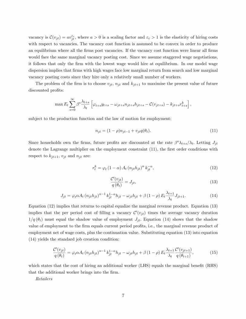
vacancy is C(vjt) = av"cjt ; where a > 0 is a scaling factor and "c > 1 is the elasticity of hiring costswith respect to vacancies: The vacancy cost function is assumed to be convex in order to produce
an equilibrium where all the �rms post vacancies. If the vacancy cost function were linear all �rms
would face the same marginal vacancy posting cost. Since we assume staggered wage negotiations,
it follows that only the �rm with the lowest wage would hire at equilibrium. In our model wage
dispersion implies that �rms with high wages face low marginal return from search and low marginal
vacancy posting costs since they hire only a relatively small number of workers.
The problem of the �rm is to choose vjt, njt and kjt+1 to maximise the present value of future
discounted pro�ts:
maxEt
1Xs=0
�s�t+s�t
h't+syt+s � !jt+snjt+shjt+s � C(vjt+s)� kjt+srkt+s
i;
subject to the production function and the law of motion for employment:
njt = (1� �)njt�1 + vjtq(�t): (11)
Since households own the �rms, future pro�ts are discounted at the rate �s�t+s=�t: Letting Jjtdenote the Lagrange multiplier on the employment constraint (11), the �rst order conditions with
respect to kjt+1, vjt and njt are:
rkt = 't (1� �)At (njthjt)� k��jt ; (12)
C0(vjt)q (�t)
= Jjt; (13)
Jjt = 't�At (njthjt)��1 k1��jt hjt � !jthjt + � (1� �)Et
�t+1�t
Jjt+1: (14)
Equation (12) implies that returns to capital equalize the marginal revenue product. Equation (13)
implies that the per period cost of �lling a vacancy C0(vjt) times the average vacancy duration1=q (�t) must equal the shadow value of employment Jjt: Equation (14) shows that the shadow
value of employment to the �rm equals current period pro�ts, i.e., the marginal revenue product of
employment net of wage costs, plus the continuation value. Substituting equation (13) into equation
(14) yields the standard job creation condition:
C0(vjt)q (�t)
= 't�At (njthjt)��1 k1��jt hjt � !jthjt + � (1� �)Et
�t+1�t
C0(vjt+1)q (�t+1)
; (15)
which states that the cost of hiring an additional worker (LHS) equals the marginal bene�t (RHS)
that the additional worker brings into the �rm.
Retailers
7
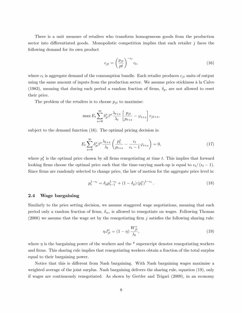
There is a unit measure of retailers who transform homogeneous goods from the production
sector into di¤erentiated goods. Monopolistic competition implies that each retailer j faces the
following demand for its own product
cjt =
�pjtpt
���tct; (16)
where ct is aggregate demand of the consumption bundle. Each retailer produces cjt units of output
using the same amount of inputs from the production sector. We assume price stickiness à la Calvo
(1983), meaning that during each period a random fraction of �rms, �p, are not allowed to reset
their price.
The problem of the retailers is to choose pjt to maximise:
maxEt
1Xs=0
�sp�s�t+s�t
�pjtpt+s
� 't+s�cjt+s;
subject to the demand function (16). The optimal pricing decision is:
Et
1Xs=0
�sp�s�t+s�t
�p�tpt+s
� �t�t � 1
't+s
�= 0; (17)
where p�t is the optimal price chosen by all �rms renegotiating at time t. This implies that forward
looking �rms choose the optimal price such that the time-varying mark-up is equal to �t= (�t � 1).Since �rms are randomly selected to change price, the law of motion for the aggregate price level is:
p1��tt = �pp1��tt�1 + (1� �p) (p�t )
1��t : (18)
2.4 Wage bargaining
Similarly to the price setting decision, we assume staggered wage negotiations, meaning that each
period only a random fraction of �rms, �w, is allowed to renegotiate on wages. Following Thomas
(2008) we assume that the wage set by the renegotiating �rm j satis�es the following sharing rule:
�J�jt = (1� �)W �jt
�t; (19)
where � is the bargaining power of the workers and the * superscript denotes renegotiating workers
and �rms. This sharing rule implies that renegotiating workers obtain a fraction of the total surplus
equal to their bargaining power.
Notice that this is di¤erent from Nash bargaining. With Nash bargaining wages maximise a
weighted average of the joint surplus. Nash bargaining delivers the sharing rule, equation (19), only
if wages are continuously renegotiated. As shown by Gertler and Trigari (2009), in an economy
8

with staggered wage negotiations Nash bargaining implies that, in the presence of staggered wage
negotiations, the share parameter � in equation (19) �uctuates over the cycle. This follows from the
fact that workers and �rms face di¤erent time horizons when they consider the e¤ects of di¤erent
wages. However, Gertler and Trigari (2009) suggest that this �horizon e¤ect� has quantitatively
negligible implications. We therefore choose to follow Thomas (2008) and adopt the sharing rule
in equation (19) as it simpli�es the analysis considerably.
With staggered wage negotiations, the shadow value of employment at �rm j to the household
that is allowed to renegotiate can be rewritten from equation (10) as follows:
W �jt
�t= !�jthjt � ~!jt + �Et
�t+1�t
(1� �)��wWjt+1jt�t+1
� (1� �w)W �jt+1
�t+1
�; (20)
where the worker�s opportunity cost of holding the job, ~!jt, is equal to:
~!jt = b+�t�t�t
h1+�jt
1 + �+ �Et
�t+1�t
(1� �) �t+1q(�t+1)Wt+1
�t:
The net value of employment to the household conditional on wage renegotiation at time t (eq.
(20)), equals the net �ow income from employment, !�jthjt� ~!jt, plus the continuation value, whichis the last term on the RHS. The latter is equal to the sum of the marginal discounted value
of employment in t + 1 conditional on the wage set a time t, if the �rm does not renegotiate with
probability �w, and the value of employment in t+1 conditional on a renegotiation, with probability
1� �w: Similarly, the shadow value of employment to the renegotiating �rm j can be written:
J�jt = �!jt � !�jthjt + (1� �)Et�t+1�t
��wJjt+1jt + (1� �w)J�jt+1
�: (21)
where �!jt = 'tmplthjt denotes the marginal revenue product: The marginal value of employment
for a renegotiating �rm equals the net �ow value of the match plus the continuation value. In turn,
this equals the marginal value of employment in t+1 conditional on the previous period wage, with
probability �w, and the marginal value conditional on a wage renegotiation, with probability 1��w.Iterating equations (20) and (21) forward it is possible to rewrite them as follows:
W �jt
�t= Et
1Xs=0
�s�t+s�t
(1� �)s�sw�!�jthjt+s � ~!jt+s
�
+(1� �)(1� �w)Et1Xs=0
�s+1�t+s+1�t
(1� �)s�swW �jt+s+1
�t+s+1; (22)
J�jt = Et
1Xs=0
�s�t+s�t
(1� �)s�sw��!jt+s � !�jthjt+s
�
9
+(1� �)(1� �w)Et1Xs=0
�s+1�t+s+1�t
(1� �)s�swJ�jt+s+1: (23)
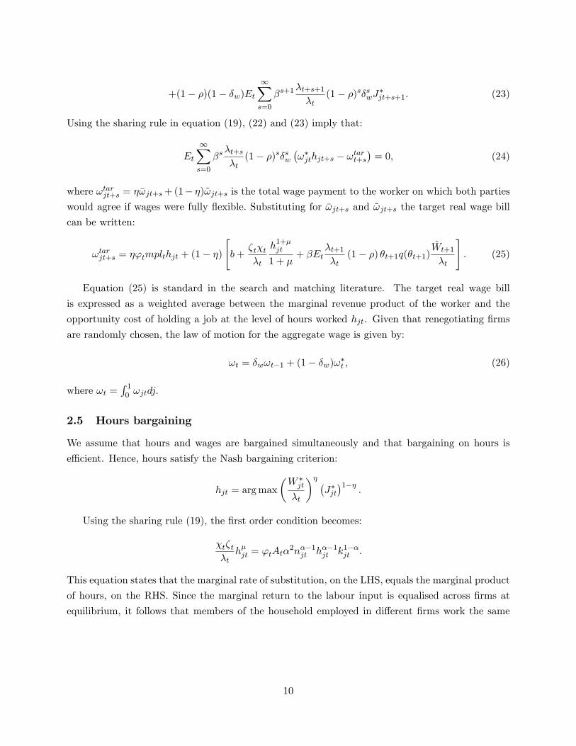
Using the sharing rule in equation (19), (22) and (23) imply that:
Et
1Xs=0
�s�t+s�t
(1� �)s�sw�!�jthjt+s � !tart+s
�= 0; (24)
where !tarjt+s = ��!jt+s+(1� �)~!jt+s is the total wage payment to the worker on which both partieswould agree if wages were fully �exible: Substituting for �!jt+s and ~!jt+s the target real wage bill
can be written:
!tarjt+s = �'tmplthjt + (1� �)"b+
�t�t�t
h1+�jt
1 + �+ �Et
�t+1�t
(1� �) �t+1q(�t+1)Wt+1
�t
#: (25)
Equation (25) is standard in the search and matching literature. The target real wage bill
is expressed as a weighted average between the marginal revenue product of the worker and the
opportunity cost of holding a job at the level of hours worked hjt. Given that renegotiating �rms
are randomly chosen, the law of motion for the aggregate wage is given by:
!t = �w!t�1 + (1� �w)!�t ; (26)
where !t =R 10 !jtdj:
2.5 Hours bargaining
We assume that hours and wages are bargained simultaneously and that bargaining on hours is
e¢ cient. Hence, hours satisfy the Nash bargaining criterion:
hjt = argmax
�W �jt
�t
�� �J�jt�1��
:
Using the sharing rule (19), the �rst order condition becomes:
�t�t�th�jt = 'tAt�
2n��1jt h��1jt k1��jt :
This equation states that the marginal rate of substitution, on the LHS, equals the marginal product
of hours, on the RHS. Since the marginal return to the labour input is equalised across �rms at
equilibrium, it follows that members of the household employed in di¤erent �rms work the same
10
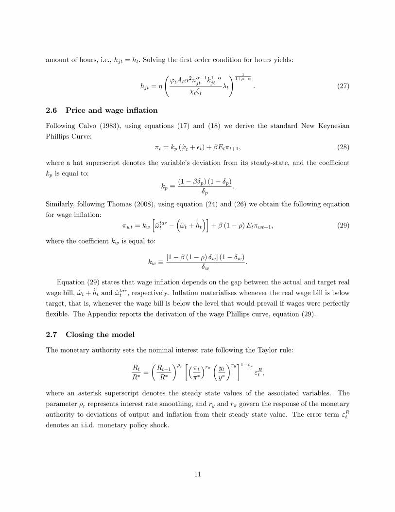
amount of hours, i.e., hjt = ht: Solving the �rst order condition for hours yields:
hjt = �
'tAt�
2n��1jt k1��jt
�t�t�t
! 11+���
: (27)
2.6 Price and wage in�ation
Following Calvo (1983), using equations (17) and (18) we derive the standard New Keynesian
Phillips Curve:
�t = kp ('t + �t) + �Et�t+1; (28)
where a hat superscript denotes the variable�s deviation from its steady-state, and the coe¢ cient
kp is equal to:
kp �(1� ��p) (1� �p)
�p:
Similarly, following Thomas (2008), using equation (24) and (26) we obtain the following equation
for wage in�ation:
�wt = kw
h!tart �
�!t + ht
�i+ � (1� �)Et�wt+1; (29)
where the coe¢ cient kw is equal to:
kw �[1� � (1� �) �w] (1� �w)
�w:
Equation (29) states that wage in�ation depends on the gap between the actual and target real
wage bill, !t + ht and !tart , respectively. In�ation materialises whenever the real wage bill is below
target, that is, whenever the wage bill is below the level that would prevail if wages were perfectly
�exible. The Appendix reports the derivation of the wage Phillips curve, equation (29).
2.7 Closing the model
The monetary authority sets the nominal interest rate following the Taylor rule:
RtR�
=
�Rt�1R�
��r ���t��
�r� � yty�
�ry�1��r"Rt ;
where an asterisk superscript denotes the steady state values of the associated variables. The
parameter �r represents interest rate smoothing, and ry and r� govern the response of the monetary
authority to deviations of output and in�ation from their steady state value. The error term "Rt
denotes an i.i.d. monetary policy shock.
11

The �scal authority is assumed to run a balanced budget:
Btpt= Rt�1
Bt�1pt
+ Tt + b (1� nt) :
2.8 Marginal costs
In this section we compare the speci�cation of marginal costs in our model against alternative
formulations in the literature. This is important to unveil some key properties of the model and
understand the �ndings detailed in the next section. Trigari (2006) shows that whenever �rms post
vacancies at time t to control employment in the following period, the matching model with e¢ cient
bargaining on hours lacks a transmission channel from wages to prices since the real marginal cost
is independent from wages. The intuition is straightforward. Since current hires contribute to next
period employment, in the current period �rms can change production only by adjusting hours. This
implies that the marginal cost of production depends solely on hours. With e¢ cient bargaining the
number of hours worked is determined by the marginal rate of substitution between consumption
and leisure and the marginal product of labour, and therefore it is independent from wages. It
follows that wages are irrelevant for marginal costs.
Following Trigari (2006), a number of authors such as Christo¤el and Kuester (2008), Christo¤el
and Linzert (2006), Mattesini and Rossi (2009) and Zanetti (2007b) have restored the transmission
channel from wages to prices by resorting to alternative bargaining schemes such as the right
to manage. In our model we are able to restore a wage channel while preserving e¢ cient Nash
bargaining. We do so by changing the timing assumption of the matching function. That is, we
allow �rms to control employment at time t by choosing vacancies in the same period, as described
by equation (11). Under this timing assumption, the cost of increasing production at the margin
depends on the cost of hiring an additional worker, which is represented by the wage paid to the
new hire. This can be seen by solving the job creation condition in equation (14) for marginal costs
't:
't =!thtmpet
+Jt � �Et �t+1�t
(1� �) Jjt+1mpet
; (30)
wherempet = At� (njthjt)��1 k1��jt hjt denotes the marginal product of employment. From equation
(30), as shown by Krause and Lubik (2007), real marginal costs are equal to the sum of the unit
labour cost and an additional term related to matching frictions. Given that the shadow value of
employment Jt equals the expected hiring cost, the second term on the RHS of equation (30) can
be interpreted as the expected change in search costs. By equation (13), this term depends on the
expected value of labour market tightness in the next period relative to the current period. If we
had assumed that newly hired workers were unable to contribute to production immediately, the
decision on vacancies would only a¤ect next period marginal costs, leaving current period marginal
costs depend solely on the number of hours, which, due to e¢ cient wage bargaining, are independent
12

from wages.
3 Estimation
The model is estimated with Bayesian methods. It is �rst loglinearised around the deterministic
steady state. We then solve the model and apply the Kalman �lter to evaluate the likelihood function
of the observable variables. The likelihood function and the prior distribution of the parameters are
combined to obtain the posterior distributions. The posterior kernel is simulated numerically using
the Metropolis-Hasting algorithm. We �rst discuss the data and the priors used in the estimation
and then report the parameter estimates.
3.1 Priors and data
The model is estimated over the period 1975Q1-2009Q1 using �ve shocks and �ve data series. We
use quarterly observations of real output scaled by the labour force. Real GDP is measured as
seasonally adjusted gross value added at basic prices. In�ation is measured as percentage changes
of the implied GDP de�ator. We also use series on average hours, employment in heads and Bank
rates. All series, with the exception of the Bank rate, are passed through a Hodrick-Prescott �lter
with smoothing parameter 1600.
The �ve shocks in the model are a preference shock, a mark-up shock, a labour supply shock, a
technology shock and a monetary policy shock. All shocks, with the exception of monetary policy
shock, are assumed to follow a �rst-order autoregressive process with i.i.d. normal error terms such
that ln�t+1 = �� ln�t + �t, where the shock � 2 f�; �; �; Ag, 0 < �� < 1 and �t � N (0; ��) :
Monetary policy shocks "Rt are i.i.d.
Some parameters are �xed, while other are estimated. We start by discussing the �xed parame-
ters. The discount factor � is set at 0.99 implying a real interest rate of 4%. Capital depreciation
�k is set at 0.025, to match an average annual rate of capital destruction of 10%, and � at 0.69 to
match the labour share over the period of the estimation. The habits parameter, &, the bargaining
power of the workers, �, and the elasticity of the vacancy cost function, "c, are also �xed, due to
identi�cation problems. Consequently, the habits parameter is then calibrated at 0.5, a value lying
in the mid range of the estimates reported in the literature for the UK economy, as detailed in
Harrison, and Oomen (2009). The bargaining power of the workers is set at 0.5, in line with the
estimates in Petrongolo and Pissarides (2001). The elasticity of the vacancy cost function is set
at 1.1, a value which is relatively close to the standard assumption of linear adjustment costs, and
satis�es the assumption of convexity. Table A summarises the values of the �xed parameters.
The remaining parameters are all estimated. We use the beta distribution for parameters that
take sensible values between zero and one, the gamma distribution for coe¢ cients restricted to be
positive and the inverse gamma distribution for the shock variances. Tables B and C report priors,
13

posterior estimates and 90% con�dence intervals.
The unemployment bene�ts coe¢ cient, b, is calibrated to match a replacement ratio of 0:38 as
in Nickell (1997). This parameter is important to generate ampli�cation of labour market variables.
As shown by Hagedorn and Manovskii (2008), values of b close to unity generate responses of
unemployment and vacancies to productivity shocks that are close to the data. When b is high, the
value of a job to the worker is very close to the value of unemployment. In this case the surplus of
a job is very small and tiny changes in the productivity of the labour input produce a high change
in the total surplus of a match, boosting the response of employment. However, as detailed below,
Costain and Reiter (2008) show that a high value of b is empirically implausible. For this reason we
choose a prior value for b which is low enough not to generate an additional source of ampli�cation.
The prior of the elasticity of the matching function, �, is set to 0:7, as estimated by Petrongolo
and Pissarides (2001) for the UK economy. The constant of the matching function, m, is normalised
to 1. The prior mean of the job destruction rate, �, is set to 0:03, in line with the estimates from
the Labour Force Survey in Bell and Smith (2002).
The Calvo parameter on wages, �!, is set to match a yearly average wage renegotiation frequency,
as in Dickens et al. (2007). Similarly, the Calvo parameter on prices, �p, is chosen to match an
average duration of prices of about six months, in line with the �ndings by Bunn and Ellis (2009)
for the UK economy. The elasticity of demand, �, is set to 11, a value suggested in Britton, Larsen
and Small (2000), which implies a steady state mark-up of 10%.
Finally, we choose the prior mean of the Taylor rule response to in�ation, r� = 1:5, and to output
ry = 0:5: While the former value is standard in the literature, the latter is somewhat higher than
the typically reported values. Our reason for a relatively high value of ry lies in the identi�cation
problems related to the use of more moderate priors. The model favours high values for ry and does
not appear to be identi�ed for relatively low values of this prior. The prior mean of the interest
rate smoothing parameter is set to 0.5.
3.2 Parameter estimates
Table B shows posterior means of the structural parameters together with 90% con�dence intervals.
The posterior mean of the unemployment bene�t parameter equal to 0.6 is substantially di¤erent
from its prior of 0.38. At the estimated equilibrium, the replacement ratio, computed as the sum of
unemployment bene�ts and the disutility of working over the wage, equals 0.77. This is remarkably
close to the value of 0.75 suggested by Costain and Reiter (2008), which is consistent with an
estimated semielasticity of unemployment to unemployment bene�ts around 2. This result suggests
that a high opportunity cost of working is unlikely to be a valid explanation for the unemployment
volatility puzzle, which is in line with the results obtained by Krause et al. (2008a) for the US
economy.
The estimate of the inverse Frish elasticity of labour supply of 1.5 is considerably higher than
14

the prior, and in line with microeconometric estimates. Since we use data on average hours, the
parameter appears to be well identi�ed. The high estimate re�ects the fact that employment
volatility is higher at the extensive margin than at the intensive margin. Krause et al. (2008a)
obtain similar results for the US, although their estimate for � is higher than ours.
The posterior means of the constant of the matching function, m, equal to 0.92 and the constant
of the vacancy cost function, a, equal to 6.5 are similar to their prior means. The posterior mean of
the rate of job separations, �; which is approximately equal to 0.7, is substantially higher than its
prior. These results imply a higher rate of unemployment than under our baseline calibration. The
unemployment rate implied by our estimated model is around 19%. This is substantially higher than
the average rate measured in the Labour Force Survey in the period 1975Q1-2009Q1. However, since
our model abstracts from the participation margin, the rate of unemployment can be interpreted as
including workers who are passively searching and are not included in the standard International
Labour Organization de�nition. In the calibration of matching models a wide range of values is
used and a rate of 19% would not be unprecedented. Trigari (2006) matches an unemployment rate
as high as 20% for the US economy.
The posterior distribution of the matching function elasticity, �, is equal to 0.55, which is
signi�cantly lower than its prior. This is evidence that the parameter is well identi�ed. The value
of 0.55 is close to the standard value 0.5 used in US studies, and inside the range of plausible values
� 2 [0:5; 0:7] estimated by Petrongolo and Pissarides (2001). This low estimate suggests that thenumber of new hires equally depend on the number of unemployed workers as well the number of
vacancies posted.
The posterior means of the Calvo parameters on the frequency of wage and price adjustments,
�! and �p, are equal to 0.75 and 0.5 respectively. These values imply an average frequency of wage
negotiations in the estimated model is one year, in line with Dickens et al. (2007), and an average
frequency of price negotiations is six months, in line with Bunn and Ellis (2009) for the UK economy.
Clearly, the estimation is unable to identify these parameters precisely as the posterior and prior
means are similar, irrespective from the assumed priors.
The parameters in the Taylor rule are well identi�ed. The posterior mean of the interest rate
response to in�ation, r�, equal to 1.46 indicates a strong response to in�ation and the degree of
interest rate smoothing, �r, equal to 0.47 suggests mild degree of interest rate inertia. Somewhat
more surprising the high estimate for ry, equal to 0.78 suggests a strong response to output. The
estimated value is larger than the typical value of 0.125, and this is obtained despite an already
large prior of 0.5. Imposing lower priors impaired the identi�cation of the model.
Table C shows estimates of the shock parameters. The posterior means of the persistence
parameters �� and �� , equal to 0.95 and 0.99 respectively, show that shocks to the labour supply
and preferences are highly persistent, while the estimates of �� and �a, equal to 0.32 and 0.69
respectively, display lower persistence of the mark-up and technology shocks. The posterior means
of �� , �a and ��, equal to 0.015, 0.008 and 0.013 respectively, show that the variances of the
15
preference, technology and monetary policy shocks are of a similar magnitude, while the estimates
of �� and �R, equal to 0.31, 0.21 respectively, display substantial higher variance of labour supply
and mark-up shocks. Both the values of the persistence and standard deviation of shocks are well
identi�ed, with the posterior distributions being largely shifted from the priors. Interestingly, the
persistence of the preference shock is close to unity, suggesting that despite wage rigidities the
model lacks an internal mechanism of propagation and requires persistence in the underlying shocks
in order to match in�ation persistence.
We now discuss how the parameter estimates change when we impose �exible wages, while
keeping the priors unchanged. The estimates are in Tables D and E. Table D shows that the
constant of the vacancy cost function is lower than in the sticky wage economy, while the constant
of the matching function and the job destruction rate are higher. This implies higher turn over
at the stationary equilibrium than we estimate in the sticky wages economy. The posterior mean
of unemployment bene�ts parameter is well identi�ed and somewhat higher than in the sticky
wage economy. All other estimates remain substantially unchanged. Importantly, the estimation
reveals that the model with sticky wages is preferred to the model with �exible wages by about 17
likelihood points. (The likelihood is 2053 for the �exible wages economy and 2070 for the sticky
wages economy).
4 Impulse response functions, variance decomposition and unob-
served shocks
In this section we investigate by use of impulse responses how the shocks are transmitted to the
endogenous variables. In order to disentangle the e¤ect of nominal wage rigidities we use both our
baseline model and the model estimated under �exible wages.
Figures 1-5 plot the impulse responses of selected variables to a one-standard-deviation shock.
Each entry compares the responses of the model with �exible wages against those with sticky
wages. Figure 1 shows that output raises in reaction to a positive technology shock and, due to the
downward sloping demand curve, prices and in�ation fall. Lower in�ation triggers a lower nominal
interest rate, which fosters consumption and investment. The qualitative reactions of these variables
are similar in the �exible and staggered wage models. On the contrary, the presence of staggered
wage setting introduces important di¤erences in the reaction of labour market variables.
Following the shock, real wages increase by more in the presence of nominal wage rigidities.
With sticky wages, price de�ation translates into higher real wages. With �exible wages, nominal
wages fall, tempering the increase in real wages. It is noticeable that vacancies, employment and
labour market tightness fall in the presence of sticky wages, while they raise when wages are �exible.
The intuition for this is straightforward. A technology shock increases both the marginal product
of labour and the real wage. The di¤erence between these two determines the incentives for posting
16
vacancies, as dictated by equation (15). With sticky wages, real wages increase by more than the
marginal product of labour, and remain elevated during the sluggish process of adjustment. With
�exible wages instead, real wages increase below the marginal product of labour and freely adjust
in the aftermath of the shock, preserving the �rms�incentives to post vacancies.
Even though wage rigidities a¤ect the transmission of technology shocks to labour market vari-
ables they are unable to produce sizeable changes to the dynamics of in�ation. Why is in�ation
dynamics similar in the two settings? As detailed in Section 2.8, search frictions introduce an addi-
tional term into marginal costs, over and above unit labour costs, which re�ects the expected change
in search costs. Following a positive technology shock, nominal wage rigidities attenuate the drop
in unit labour costs and amplify the fall in the frictional component of marginal costs compared
to a �exible wage regime. As a result, marginal costs and in�ation dynamics behave similarly in
the two settings. Wage rigidities attenuate the reaction of unit labour costs since real wages hold
up on impact as �rms are not allowed to renegotiate lower wages. At the same time, as mentioned
above, wage rigidities induce labour market tightness to fall on impact and then steadily increase.
As a result, the �rm�s cost of searching for a worker falls on impact and it then raises over time.5
The rising pro�le in expected search costs implies that the �rm can save on future hiring costs by
increasing current period hiring. From equation (30), higher expected search costs next period,
translate in lower marginal costs in the current period. As a result, the impact of wage rigidities
on the frictional component of marginal costs compensates the impact on unit labour costs, leaving
total marginal costs unchanged compared to the case of �exible wages.
Figure 2 shows that a one-standard-deviation mark-up shock leads to an increase in in�ation.
As the interest rate increases, consumption and investment fall. In reaction to the shock, the �rm
reduces the labour input along both the intensive and the extensive margin to decrease production.
Note that the qualitative responses of the variables in the staggered wage model are similar to those
in the model with �exible wage setting, since mark-up shocks do not induce the �rm to adjust labour
market variables di¤erently, as in the case of technology shocks. Nonetheless, similarly to the case
of technology shocks, the reaction of marginal costs and in�ation remains substantially unchanged
in the two settings.
Figure 3 shows that one-standard-deviation labour supply shock reduces hours and exerts upward
pressure on nominal wages by increasing the disutility of work. With �exible nominal wages, real
wages increase, leading to a reduction in vacancies and employment. On the contrary, with staggered
wage bargaining nominal wage in�ation is lower than price in�ation, which implies that real wages
fall. Consequently, in the sticky wage model, vacancies and employment increase. With continuous
wage negotiations higher nominal wage in�ation translates into higher price in�ation, which leads
to higher interest rates and lower consumption and investment. Wage rigidities appear to have
somewhat sizeable impact on marginal costs since the e¤ect produced through unit labour costs is
only partially o¤set by the e¤ect of the frictional component of marginal costs.5Note that the average duration of a vacancy, 1=q(�t), depends only on labour market tightness.
17
Figure 4 shows that a one-standard-deviation monetary policy shock causes an increase in the
nominal interest rate, and a fall in both in�ation and output. As in the cases of mark-up shocks,
nominal wage rigidities do not alter the qualitative responses of the variables on impact, with the
exception of the reaction of real wages. In both settings, in reaction to the shock, vacancies and
employment fall, while in the presence of sticky wages price de�ation generates higher real wages.
When wages are continuously renegotiated instead, nominal wages fall at a faster pace than prices
and real wages fall. Once again nominal wage rigidities have a di¤erent impact on unit labour costs
in the two settings, whose movements are o¤set by the reaction of search costs. This generates
similar marginal costs and price in�ation in the two settings.
Figure 5 shows impulse responses to a one-standard-deviation preference shock. The qualitative
responses of the variables are the same for the sticky and �exible settings. The preference shock
generates an increase in consumption and upward pressure on prices. As price in�ation increases,
the nominal interest rate raises, and both investment and output fall. The preference shock induces
the worker to work a lower number of hours, thereby generating lower return from employment.
Hence, the �rm posts fewer vacancies, contracting employment and labour market tightness. Finally,
also in this instance, nominal wage rigidities produce only a minor impact on marginal costs, since
search friction costs o¤set movements in unit labour costs. As a result, in�ation dynamics remain
similar with and without staggered wage settings.
To summarize, we �nd that while wage rigidities might a¤ect the response of labour market
variables, they are substantially irrelevant for the dynamics of in�ation. This echoes the �ndings
in Krause and Lubik (2007), who reached a similar conclusion in a calibrated model with an ad-
hoc staggered wage setting and fewer shocks. This is in stark contrast with the predictions of the
standard New Keynesian model without labour market frictions, as in Christiano et al. (2005).
In their model unit labour costs are the only determinant of marginal costs, implying that wage
rigidities naturally generate in�ation persistence. Our analysis shows that in a model with search
frictions, the contribution of unit labour costs for marginal costs is o¤set by movements in search
costs, which become an additional component of marginal costs. However, this �nding is at odds
with the results obtained by Gertler et al. (2008), who estimate a similar model on the US economy
and �nd that wage rigidities are important for the dynamics of in�ation. This suggests that the
link between in�ation and marginal costs might depend on the estimated parameter values, and in
particular on the degree of nominal wage and price rigidities. Future studies should investigate this
issue further.
To understand the extent to which cyclical movements of each variable are explained by the
shocks, Table F reports the variance decompositions for the model with sticky wages. Entries reveal
that most of the movements in the model�s variables are driven by preference shocks. Preference
shocks exhibit an autocorrelation coe¢ cient of 0.99, as detailed in Table C, which is higher than in
all other shocks, and therefore magni�es the importance of preference shocks. This suggests that the
model has a weak internal propagation mechanism and the �uctuation of the endogenous variables
18

heavily depends on extrinsic sources of persistence, similarly to Krause et al. (2008a). However,
while in Krause et al. (2008a) in�ation persistence is generated by a number of shocks, in our
model preference shocks are the main source of persistence. In addition, since the persistence of the
preference shock is equally large both in the sticky and in the �exible wage model, we conclude that
wage rigidities alone are unable to produce in�ation persistence. Table F also shows that mark-up
shocks play a limited role in explaining movements of variables, suggesting that demand shocks are
the main driver of economic �uctuations in the UK. Labour supply shocks appear to play a role,
albeit a minor one, in driving vacancies and employment. Hours instead are mostly driven by labour
supply shocks.
To detail how the exogenous shocks have evolved during the estimation period, Figure 6 plots
shocks estimates using the Kalman smoothing algorithm from the state-space representation of the
estimated model with sticky wages. The estimates show that the magnitude of shocks has somewhat
decreased since the mid-1990s, with the exception of preferences shocks, whose size has remained
broadly unchanged. Furthermore, similarly to studies for other countries, we �nd that the volatility
of monetary policy shocks declined after the mid-1990s. These �ndings corroborate the results of
empirical studies, such as Benati (2007) and Bianchi et al. (2009), which detected a period of
macroeconomic stability triggered by a lower volatility of shocks in the UK during the past decade.
5 Conclusion
We have estimated a New Keynesian model characterized by labour market frictions on UK data to
identify some key features of the UK economy. First, we estimated important structural parameters
of the British economy, which enabled the investigation of the transmission mechanism of shocks
and how it changes due to wage rigidities. We established that shocks to preferences and the labour
supply are more important than technology, monetary policy, or mark-up shocks in explaining
movements in the data. In addition, using a Kalman �lter on the model�s reduced form we provided
estimates for the unobserved shocks that characterised the post 1970s British economy. Similarly
to studies for other countries, we found that the volatility of shocks declined after the mid-1990s,
corroborating the evidence that this factor might have contributed to the macroeconomic stability
of the past decade.
Second, we established that staggered wage setting a¤ects the behaviour of labour market vari-
ables and enables the model to �t the data more closely, despite playing an irrelevant role for the
dynamics of in�ation. In a search and matching model the marginal cost depends on the unit labor
cost as well as on the frictional costs of searching. We show that introducing wage rigidities into
an otherwise identical model with �exible wages generates o¤setting reactions in the frictional costs
of employment and in the unit labor cost. As a result, in�ation dynamics remain substantially
una¤ected. This �nding, which echoes the results by Krause and Lubik (2007), is obtained despite
establishing a link between wage and in�ation by assuming that newly hired workers become im-
19
mediately productive. However, this result is in contrast to Gertler et al. (2008), who, using a
similar timing assumption, �nd that wage rigidities a¤ect in�ation dynamics in a model estimated
on the US. This discrepancy suggests that future research should investigate the role of the esti-
mated parameter values in determining the link between in�ation and marginal costs. Furthermore,
the �nding is also di¤erent from studies that have restored the transmission channel from wages
to prices by resorting to alternative wage bargaining schemes, such as right-to-manage bargaining.
Future research needs to establish what bargaining scheme the data support more strongly.
While the results do unveil key features of the UK economy, it should also be noted that the
estimation was unable to precisely identify important parameters of the model, such as the degree
of nominal wage and price adjustments, calling for re�nements to the theoretical setting that could
improve the empirical performance of the model. Furthermore, although the model developed here
allows for a variety of supply and demand shocks to have e¤ects on the economy, in practice, a
variety of other aggregate shocks may play a role. The amendment of the model and the inclusion
of additional disturbances remain outstanding tasks for future research.
20
References
[1] Andolfatto, D. (1996). �Business Cycles and Labour Market Search�, American Economic
Review 86, 112-132.
[2] Bean, C. R. (1994). �European unemployment: a survey�, Journal of Economic Literature, 32,
573-619.
[3] Bell, B., and Smith, J., (2002). �On gross worker �ows in the United Kingdom: evidence from
the Labour Force Survey�, Bank of England Woking Paper 160.
[4] Benati, L. (2007). �The Great Moderation in the United Kingdom�, Journal of Money, Credit
and Banking, 39(1), 121-147.
[5] Bianchi, F., Mumtaz, H. and Surico, P. (2009). �The great Moderation of the Term Structure
of UK Interest Rates�, Journal of Monetary Economics, 56(6), 749-906.
[6] Britton, E., Larsen, J. D., and Small, I., (2000). �Imperfect competition and the dynamics of
mark-ups�, Bank of England Working Paper 110.
[7] Bunn, P. and Ellis, C. (2009). �Price-setting behaviour in the United Kingdom: a microdata
approach�, Bank of England Quarterly Bullettin 2009 Q1.
[8] Calvo, G. (1983). �Staggered Contracts in a Utility Maximizing Framework�, Journal of Mon-
etary Economics 12, 383-398.
[9] Christiano, L.J., Eichenbaum, M., Evans, C., (2005). �Nominal Rigidities and the Dynamic
E¤ects of a Shock to Monetary Policy�, Journal of Political Economy 105, 249-283.
[10] Christo¤el, K., Costain, J., de Walque, G., Kuester, K., Linzert, T., Millard, S. and Pierrard,
O., (2009). �In�ation dynamics with labour market matching: assessing alternative speci�ca-
tions�Working Papers 09-6, Federal Reserve Bank of Philadelphia.
[11] Christo¤el, K. and Kuester, K. (2008). �Resuscitating the wage Channel in Models with Un-
employment Fluctuations�, Journal of Monetary Economics, 55(5), 865-887.
[12] Christo¤el, K., Kuester, K. and Linzert, T. (2009). �The role of Labor Markets for Euro Area
Monetary Policy�European Economic Review, forthcoming.
[13] Christo¤el, K. and Linzert, T. (2006). �The Role of Real Wage Rigidity and Labor Market
Frictions for Unemployment and In�ation Dynamics�, Discussion Paper Series 1: Economic
Studies 2006,11, Deutsche Bundesbank, Research Centre.
21
[14] Costain, J.S., and Reiter, M. (2008). �Business Cycles, Unemployment Insurance, and the
Calibration of Matching Models�, Journal of Economic Dynamics and Control, 32(4), 1120-
1155.
[15] Dickens, W. T., Goette, L., Groshen. E. L., Holden, S., Messina, J., Schweitzer, M. E., Turunen,
J. and Ward, M. E. (2007). �How Wages Change: Micro Evidence from the International Wage
Flexibility Project�, Journal of Economic Perspectives, 21(2), 195-214.
[16] Gali, J. and Gertler, M. (1999). �In�ation Dynamics: a Structural Econometric Analysis�,
Journal of Monetary Economics 44, 195-222.
[17] Gertler, M., Sala, L. and Trigari, A. (2008). �An Estimated Monetary DSGE Model with Un-
employment and Staggered Nominal Wage Bargaining�, Journal of Money, Credit and Banking,
40(8), 1713-1764.
[18] Gertler, M. and Trigari, A. (2009). �Unemployment Fluctuations with Staggered Nash Bar-
gaining�, Journal of Political Economy, 117(1), 38-86.
[19] Harrison, R. and Oomen, O. (2009). �Evaluating and Estimating a DSGE Model for United
Kingdom�, Bank of England Working Paper, forthcoming.
[20] Hobijn, B., Sahin, A., (2007). �Job-�nding and separation rates in the OECD�, Federal Reserve
Bank of New York Sta¤ Report 298.
[21] Mattesini, F. and Rossi, L. (2008). �Optimal Monetary Policy in Economies With Dual Labor
Markets�, Journal of Economic Dynamics and Control, 33(7), 1469-1489.
[22] Merz, M. (1995). �Search in the Labor Market and the Real Business Cycle�, Journal of
Monetary Economics, 36, 269-300.
[23] Nickell, S. (1997) �Unemployment and Labor Market Rigidities: Europe versus North Amer-
ica�, Journal of Economic Perspectives, Vol.11, No.3, 55-74.
[24] Hagedorn, M., and Manovskii, I. (2008). �The Cyclical Behaviour of Equilibrium Unemploy-
ment and Vacancies Revisited�, American Economic Review, 98(4), 1692-1706.
[25] Krause, M., Lopez-Salido, D.J. and Lubik, T.A. (2008a). �In�ation Dynamics with Search
Frictions: A Structural Econometric Analysis�, Journal of Monetary Economics, 55(5), 892-
916.
[26] Krause, M., Lopez-Salido, D.J. and Lubik, T.A., (2008b). �Do Search Frictions Matter for
In�ation Dynamics?�, European Economic Review, 52(8), 1464-1479.
22
[27] Krause, M. and Lubik, T.A. (2007). �The Irrelevance of Real Wage Rigidity in the New Key-
nesian Model with Search Frictions�, Journal of Monetary Economics, 54, 706-727.
[28] Petrongolo, B. and Pissarides, C.A. (2001) �Looking into the Black Box: A Survey of the
Matching Function�, Journal of Economic Literature, 39(2),390-431.
[29] Ravenna, F. and Walsh, C.E. (2008) �Vacancies, Unemployment, and the Phillips Curve�,
European Economic Review, 52(8), 1494-1521.
[30] Smets, F. and Wouters, R. (2003). �An Estimated Dynamic Stochastic General Equilibrium
Model of the Euro Area�Journal of the European Economic Association 1(5), 527-549.
[31] Smets, F. and Wouters, R. (2007). �Shocks and Frictions in US business Cycles: a Bayesian
DSGE Approach�, American Economic Review, 97(3), 586-606.
[32] Thomas, C. (2008). �Search and Matching Frictions and Optimal Monetary Policy�, Journal
of Monetary Economics, 55, 936-956.
[33] Trigari, A. (2006). �The Role of Search Frictions and Bargaining for In�ation Dynamics�,
Working Paper 304, IGIER (Innocenzo Gasparini Institute for Economic Research), Bocconi
University.
[34] Zanetti, F. (2007a). �Labor market institutions and aggregate �uctuations in a search and
matching model�, Bank of England Working Paper, no. 333.
[35] Zanetti, F. (2007b), �A non-Walrasian labor market in a monetary model of the business cycle�,
Journal of Economic Dynamics and Control 31(7), July, 2413-2437.
23
Appendix ADerivation of the wage Phillips curve.
A �rst order Taylor expansion on (24) yields:
Et
1Xs=0
�s(1� �)s�sw�log!�jthjt+s log!h� !tarjt+sjt
�= 0: (31)
Notice from equation (25) in the text that !tarjt = !tart . If !tarjt = !tart , then equation (24) implies
that !�jt = !�t :
Equation (31) can be rewritten solving for !�t , and expressing the solution recursively:
log!�t = [1� � (1� �) �w]�!tart � log ht + log!h
�+ � (1� �) �wEt log!�t+1: (32)
The law of motion of the wage index in equation (26) can be rewritten as follows:
log!�t � log!t�1 = �wt; (33)
where �wt = log!t � log!t�1: Using (33), equation (31) can be rewritten as:
�wt = kw
�!tart � !t � ht
�+ � (1� �)Et�wt+1;
where kw = [1� � (1� �) �w] (1� �w) =�w:Appendix BThe log-linear equilibrium conditions:
Euler equations
�t = �t+1 + rt � �t+1
�t = �t � [�= (1� &)] (ct � ct�1)
�t = �t+1 + � (1� �)'
�
y
k
�'t+1 � �t+1 + yt+1 � kt+1
�Production function
yt = At + ��nt + ht
�+ (1� �) kt
Resource constraint
yt =
�c
y
�ct +
"ccv"c
yvt +
i
y{t +
g
ybgt
Unemployment
ut = �(1� �)n
unt�1
Employment
nt = (1� �)nt�1 + � [�ut + (1� �) vt]
24

Tightness
�t = vt � ut
Investmenti
k{t = kt+1 � (1� �k) kt
Job Creation
"ccv"c�1��
m
h("c � 1) vt + ��t
i= �
'
�
y
n
�cmct � �t + yt � nt�� !h�!t + ht�
+(1� �)� "ccv"c�1��
m
h("c � 1) vt+1 + ��t+1 + �t+1 � �t
iTarget wage bill
!tart =1
!h
��'mpe ('t + dmpet) + (1� �) h1+�1 + �
1
�
��t + �t � �t + (1 + �) ht
��
+� (1� �)�"ccv"c�1�h�t+1 � �t + �t+1 + ("c � 1) vt+1
iHours
ht =1
(1 + �� �)
h't + At + (�� 1) nt + (1� �) kt + �t � �t � �t
iMarginal product of employment
dmpet = At + (1� �)�kt�1 � nt�+ �ntAverage real wage
!t � !t�1 + �t = �wt
Wage in�ation
�wt = kw
�!tart � !t � ht
�+ ��t+1
Price in�ation
�t = kp ('t + �t) + ��t+1
Taylor rule
rt = �rrt�1 + (1� �r) (r��t + ryyt) + "Rt
25

Table A: Fixed Parameters
Parameters Description Values
� Discount factor 0:99
� Labour share 0:69
�k Capital depreciation rate 0:025
& Habit persistence 0:50
"c Elasticity of the vacancy cost function 1:10
� Bargaining power parameter 0:50
26
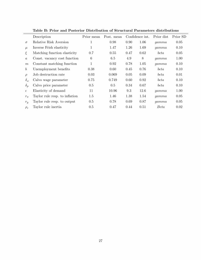
Table B: Prior and Posterior Distribution of Structural Parameters distributions
Description Prior mean Post. mean Con�dence int. Prior dist Prior SD
� Relative Risk Aversion 1 0:98 0:90 1:06 gamma 0:05
� Inverse Frish elasticity 1 1:47 1:26 1:69 gamma 0:10
� Matching function elasticity 0:7 0:55 0:47 0:62 beta 0:05
a Const. vacancy cost function 6 6:5 4:9 8 gamma 1:00
m Constant matching function 1 0:92 0:78 1:05 gamma 0:10
b Unemployment bene�ts 0:38 0:60 0:45 0:76 beta 0:10
� Job destruction rate 0:03 0:069 0:05 0:09 beta 0:01
�! Calvo wage parameter 0:75 0:749 0:60 0:92 beta 0:10
�p Calvo price parameter 0:5 0:5 0:34 0:67 beta 0:10
� Elasticity of demand 11 10:96 9:3 12:6 gamma 1:00
r� Taylor rule resp. to in�ation 1:5 1:46 1:38 1:54 gamma 0:05
ry Taylor rule resp. to output 0:5 0:78 0:69 0:87 gamma 0:05
�r Taylor rule inertia 0:5 0:47 0:44 0:51 Beta 0:02
27
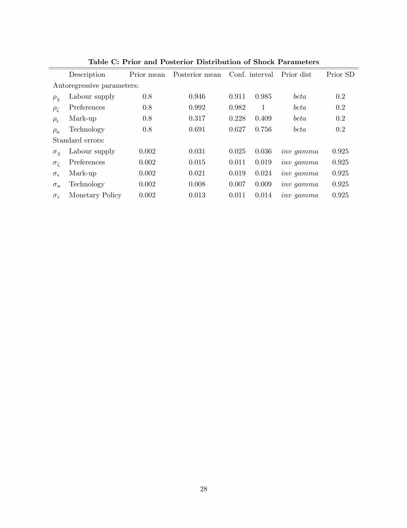
Table C: Prior and Posterior Distribution of Shock Parameters
Description Prior mean Posterior mean Conf. interval Prior dist Prior SD
Autoregressive parameters:
�� Labour supply 0:8 0:946 0:911 0:985 beta 0:2
�� Preferences 0:8 0:992 0:982 1 beta 0:2
�� Mark-up 0:8 0:317 0:228 0:409 beta 0:2
�a Technology 0:8 0:691 0:627 0:756 beta 0:2
Standard errors:
�� Labour supply 0:002 0:031 0:025 0:036 inv gamma 0:925
�� Preferences 0:002 0:015 0:011 0:019 inv gamma 0:925
�� Mark-up 0:002 0:021 0:019 0:024 inv gamma 0:925
�a Technology 0:002 0:008 0:007 0:009 inv gamma 0:925
�" Monetary Policy 0:002 0:013 0:011 0:014 inv gamma 0:925
28

Table D: Prior and Posterior Distribution of Structural Parameters distributions,�exible wages economy
Description Prior mean Post. mean Con�dence int. Prior dist Prior SD
� Relative Risk Aversion 1 0:96 0:88 1:04 gamma 0:05
� Inverse Frish elasticity 1 1:51 1:31 1:70 gamma 0:10
� Matching function elasticity 0:7 0:53 0:53 0:46 beta 0:05
a Const. vacancy cost function 6 3:7 2:8 5:0 gamma 1:00
m Constant matching function 1 1:3 1:18 1:47 gamma 0:10
b Unemployment bene�ts 0:38 0:75 0:65 0:85 beta 0:10
� Job destruction rate 0:03 0:10 0:08 0:13 beta 0:01
�! Calvo wage parameter (�xed) 0 0 - - - -
�p Calvo price parameter 0:5 0:49 0:29 0:64 beta 0:10
� Elasticity of demand 11 11:1 9:0 12:7 gamma 1:00
r� Taylor rule resp. to in�ation 1:5 1:56 1:51 1:63 gamma 0:05
ry Taylor rule resp. to output 0:5 0:69 0:62 0:77 gamma 0:05
�r Taylor rule inertia 0:5 0:47 0:44 0:50 Beta 0:02
29

Table E: Prior and Posterior Distribution of Shock Parameters, �ex wages economy
Description Prior mean Posterior mean Conf. interval Prior dist Prior SD
Autoregressive parameters:
�� Labour supply 0:8 0:999 0:975 1 beta 0:2
�� Preferences 0:8 0:999 0:988 1 beta 0:2
�� Mark-up 0:8 0:371 0:285 0:442 beta 0:2
�a Technology 0:8 0:697 0:624 0:747 beta 0:2
Standard errors:
�� Labour supply 0:002 0:024 0:020 0:028 inv gamma 0:925
�� Preferences 0:002 0:013 0:011 0:015 inv gamma 0:925
�� Mark-up 0:002 0:018 0:016 0:021 inv gamma 0:925
�a Technology 0:002 0:008 0:007 0:009 inv gamma 0:925
�" Monetary Policy 0:002 0:012 0:011 0:013 inv gamma 0:925
30

Table F: Variance decomposition
Preference Labour supply Mark-up Technology Monetary policy
r 0:92 0:08 0:04 0:00 0:00
y 0:88 0:10 0:01 0:00 0:00
� 0:90 0:09 0:00 0:00 0:00
h 0:08 0:75 0:11 0:00 0:05
i 0:84 0:10 0:02 0:02 0:00
n 0:87 0:10 0:00 0:01 0:01
v 0:75 0:15 0:02 0:02 0:06
31
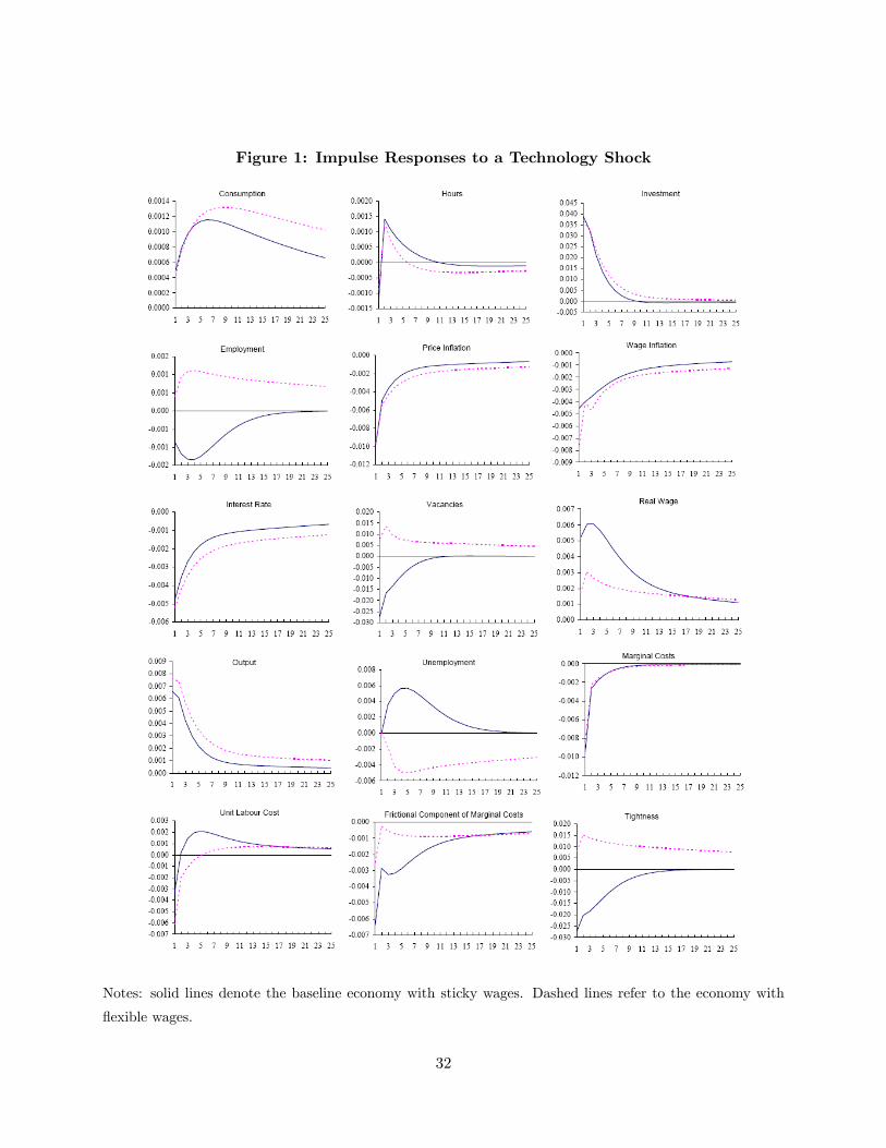
Figure 1: Impulse Responses to a Technology Shock
Notes: solid lines denote the baseline economy with sticky wages. Dashed lines refer to the economy with
�exible wages.
32
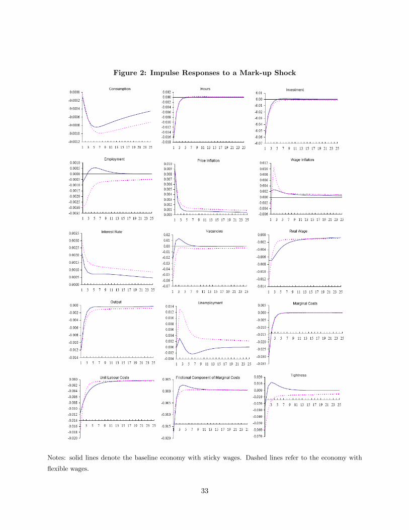
Figure 2: Impulse Responses to a Mark-up Shock
Notes: solid lines denote the baseline economy with sticky wages. Dashed lines refer to the economy with
�exible wages.
33

Figure 3: Impulse Responses to a Labour Supply Shock
Notes: solid lines denote the baseline economy with sticky wages. Dashed lines refer to the economy with
�exible wages.
34
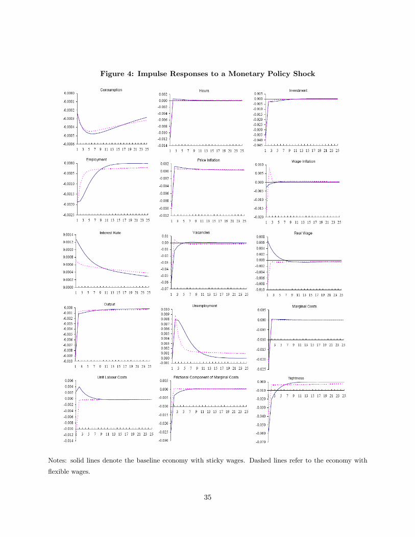
Figure 4: Impulse Responses to a Monetary Policy Shock
Notes: solid lines denote the baseline economy with sticky wages. Dashed lines refer to the economy with
�exible wages.
35
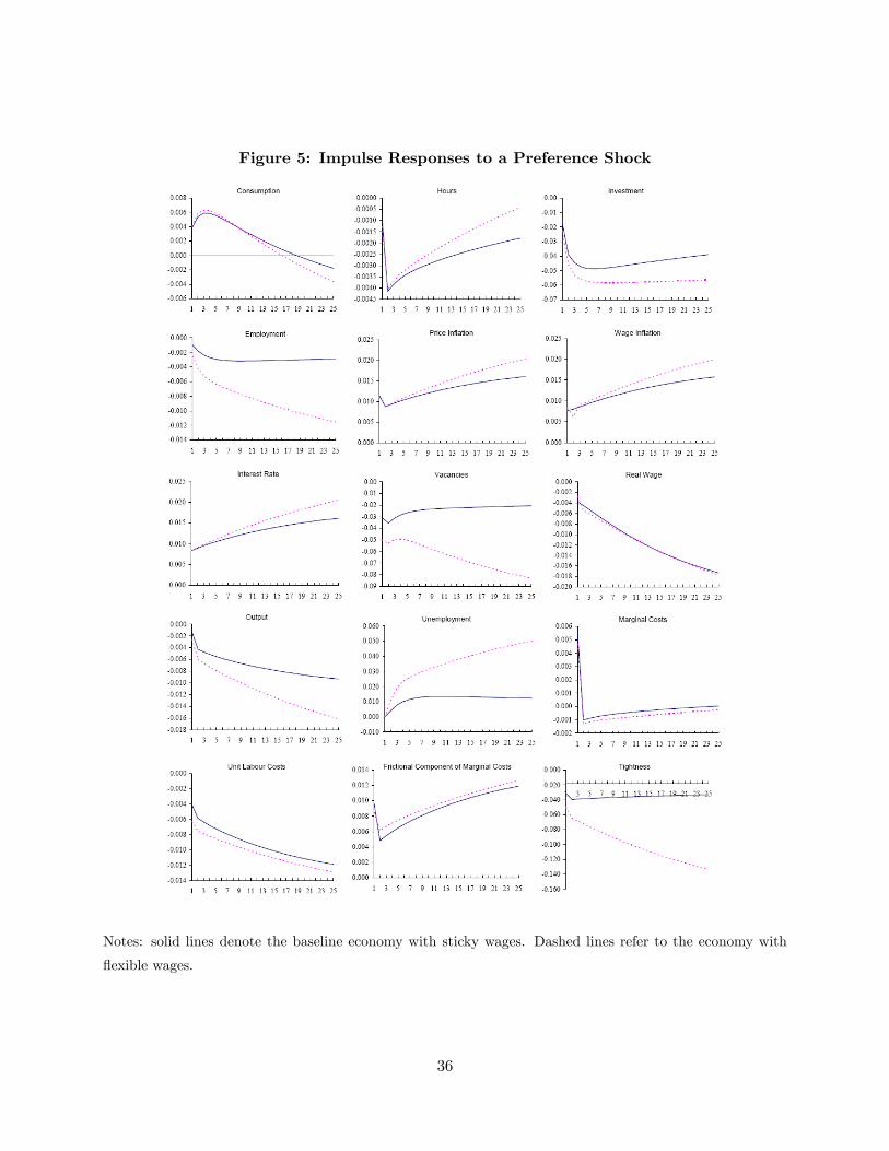
Figure 5: Impulse Responses to a Preference Shock
Notes: solid lines denote the baseline economy with sticky wages. Dashed lines refer to the economy with
�exible wages.
36

Figure 6: Smoothed Shocks
37