Embed Size (px)
Citation preview

Microfoundations of DSGE Models: III Lecture
Barbara Annicchiarico
BBLM del Dipartimento del Tesoro
21 Giugno 2010
B. Annicchiarico (Università di Tor Vergata) (Institute)Microfoundations of DSGE Models 21 Giugno 2010 1 / 65

Contents
A New Keynesian model with capital accumulationA New Keynesian model with capital accumulation, habitpersistence and adjustment costs on labour and investmentsA New Keynesian model with capital accumulation andrule-of-thumb householdsA complete model
B. Annicchiarico (Università di Tor Vergata) (Institute)Microfoundations of DSGE Models 21 Giugno 2010 2 / 65

Model #1: A NK Model with Capital AccumulationMain Features
Agentsa continuum of households that consume, own capital and supplydifferentiated labour services;a continuum of trade unions each of which representing workers ofa certain type;a continuum of intermediate goods producers that employ labourinputs, rent capital from households and produce differentiatedintermediate goods (monopolistic competition);a continuum of final goods producers that use intermediate goodsto produce a homogenous final good consumed by households(perfect competition);the government that set public spending;the central bank that implements monetary policy.
Imperfect competitionPrices rigiditiesBusiness cycles driven by nominal and real shocksRational expectations and no asymmetric information
B. Annicchiarico (Università di Tor Vergata) (Institute)Microfoundations of DSGE Models 21 Giugno 2010 3 / 65

Model #1: A NK Model with Capital AccumulationFinal-Good Firms
Each firm takes the other firms’ prices as given.The representative final-good firm uses Yt (j) units of eachintermediate good j 2 [0, 1] purchased at a nominal price Pt (j) toproduce Yt units of the final good with a constant returns to scaletechnology:
Yt =�Z 1
0Yt (j)
θ�1θ dj
� θθ�1
θ = the elasticity of substitution across intermediate goods, θ > 1. Asθ ! ∞ higher and higher degree of substitution ! less market powerof intermediate-goods producers.
B. Annicchiarico (Università di Tor Vergata) (Institute)Microfoundations of DSGE Models 21 Giugno 2010 4 / 65

Model #1: A NK Model with Capital AccumulationFinal-Good Firms
The problem of the representative firm is to max their profits wrt Yt (j) withj 2 [0, 1] (static problem) given the available technology.
PtYt �Z 1
0Pt (j)Yt (j) dj
Profit maximization yields the following set of demands for intermediategoods:
Yt (j) =�Pt (j)Pt
��θ
Yt
Perfect competition and free entry drives the final good-producing firms’profits to zero, so that from the zero-profit condition we obtain:
Pt =�Z 1
0Pt (j)
1�θ dj� 11�θ
.
which defines the aggregate price index of the economy and is such thatPtYt =
R 10 Pt (j)Yt (j) dj .
B. Annicchiarico (Università di Tor Vergata) (Institute)Microfoundations of DSGE Models 21 Giugno 2010 5 / 65

Model #1: A NK Model with Capital AccumulationIntermediate-Goods Firms
Each intermediate good j is produced by a monopolist which has aproduction function of the form:
Yt (j) = AtLt (j)αKt (j)1�α
where 0 < α < 1At = Total factor productivity, At = A exp(εA,t ) and εA,t = ρAεA,t + ξA,twith ξA,t � iid .N(0, σ2A)Lt (j) = CES aggregate of labor inputs supplied by unionized workersdefined below (see below)Kt (j) = physical capital
B. Annicchiarico (Università di Tor Vergata) (Institute)Microfoundations of DSGE Models 21 Giugno 2010 6 / 65
Model #1: A NK Model with Capital AccumulationPrice Rigidities à la Rotemberg
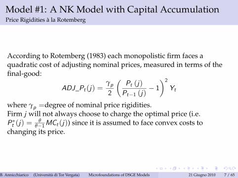
According to Rotemberg (1983) each monopolistic firm faces aquadratic cost of adjusting nominal prices, measured in terms of thefinal-good:
ADJ_Pt (j) =γp2
�Pt (j)Pt�1 (j)
� 1�2Yt
where γp =degree of nominal price rigidities.Firm j will not always choose to charge the optimal price (i.e.P�t (j) =
θθ�1MCt (j)) since it is assumed to face convex costs to
changing its price.
B. Annicchiarico (Università di Tor Vergata) (Institute)Microfoundations of DSGE Models 21 Giugno 2010 7 / 65

Model #1: A NK Model with Capital AccumulationPrice Rigidities à la Rotemberg
Why are price changes costly?
There is the cost of physically changing posted prices (probably afixed cost per price change).A firm that changes its prices may face a cost which results fromthe negative reaction of its costumers (reputation loss). From thispoint of view, probably customers react more strongly to largeprice changes than to gradual variations.
B. Annicchiarico (Università di Tor Vergata) (Institute)Microfoundations of DSGE Models 21 Giugno 2010 8 / 65
Model #1: A NK Model with Capital AccumulationPrice Rigidities à la Rotemberg
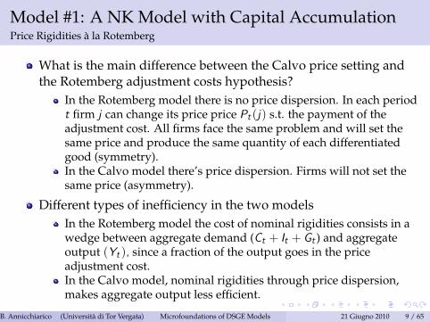
What is the main difference between the Calvo price setting andthe Rotemberg adjustment costs hypothesis?
In the Rotemberg model there is no price dispersion. In each periodt firm j can change its price price Pt (j) s.t. the payment of theadjustment cost. All firms face the same problem and will set thesame price and produce the same quantity of each differentiatedgood (symmetry).In the Calvo model there’s price dispersion. Firms will not set thesame price (asymmetry).
Different types of inefficiency in the two modelsIn the Rotemberg model the cost of nominal rigidities consists in awedge between aggregate demand (Ct + It + Gt ) and aggregateoutput (Yt ), since a fraction of the output goes in the priceadjustment cost.In the Calvo model, nominal rigidities through price dispersion,makes aggregate output less efficient.
B. Annicchiarico (Università di Tor Vergata) (Institute)Microfoundations of DSGE Models 21 Giugno 2010 9 / 65

Model #1: A NK Model with Capital AccumulationPrice Rigidities à la Rotemberg
Despite the economic difference between these two models of pricerigidities, up to a first order approximation and around a zero inflationsteady state, they imply the same reduced form of the New KeynesianPhillips curve.Otherwise, the Rotemberg model seems to be more robust tonon-linearities (implying more robust results).The implications of of having trend inflation in the two pricing models.On these issues: see Ascari and Merkl (2009); Ascari and Ropele (2007);Ascari and Rossi (2009, 2010).
B. Annicchiarico (Università di Tor Vergata) (Institute)Microfoundations of DSGE Models 21 Giugno 2010 10 / 65
Model #1: A NK Model with Capital AccumulationIntermediate-Goods Firms
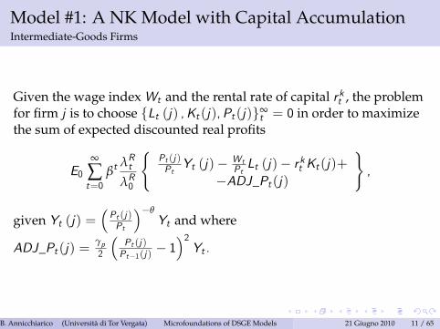
Given the wage index Wt and the rental rate of capital r kt , the problemfor firm j is to choose fLt (j) ,Kt (j),Pt (j)g∞
t = 0 in order to maximizethe sum of expected discounted real profits
E0∞
∑t=0
βtλRtλR0
(Pt (j)PtYt (j)� Wt
PtLt (j)� r kt Kt (j)+
�ADJ_Pt (j)
),
given Yt (j) =�Pt (j)Pt
��θYt and where
ADJ_Pt (j) =γp2
�Pt (j)Pt�1(j)
� 1�2Yt .
B. Annicchiarico (Università di Tor Vergata) (Institute)Microfoundations of DSGE Models 21 Giugno 2010 11 / 65
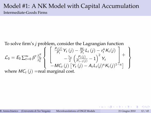
Model #1: A NK Model with Capital AccumulationIntermediate-Goods Firms
To solve firm’s j problem, consider the Lagrangian function
L0 = E0 ∑∞t=0 βt λRt
λR0
8>><>>:24 Pt (j)
PtYt (j)� Wt
PtLt (j)� r kt Kt (j)
�γp2
�Pt (j)Pt�1(j)
� 1�2Yt
35+�MCt (j)
�Yt (j)� AtLt (j)αKt (j)1�α
�9>>=>>;
where MCt (j) =real marginal cost.
B. Annicchiarico (Università di Tor Vergata) (Institute)Microfoundations of DSGE Models 21 Giugno 2010 12 / 65
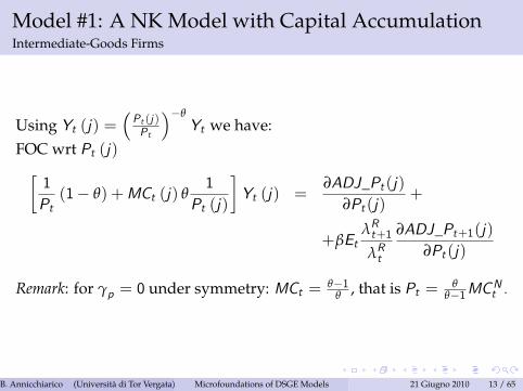
Model #1: A NK Model with Capital AccumulationIntermediate-Goods Firms
Using Yt (j) =�Pt (j)Pt
��θYt we have:
FOC wrt Pt (j)�1Pt(1� θ) +MCt (j) θ
1Pt (j)
�Yt (j) =
∂ADJ_Pt (j)∂Pt (j)
+
+βEtλRt+1
λRt
∂ADJ_Pt+1(j)∂Pt (j)
Remark: for γp = 0 under symmetry: MCt = θ�1θ , that is Pt = θ
θ�1MCNt .
B. Annicchiarico (Università di Tor Vergata) (Institute)Microfoundations of DSGE Models 21 Giugno 2010 13 / 65
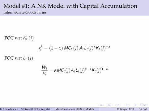
Model #1: A NK Model with Capital AccumulationIntermediate-Goods Firms
FOC wrt Kt (j)
r kt = (1� α)MCt (j)AtLt (j)αKt (j)�α
FOC wrt Lt (j)
Wt
Pt= αMCt (j)AtLt (j)α�1Kt (j)1�α
B. Annicchiarico (Università di Tor Vergata) (Institute)Microfoundations of DSGE Models 21 Giugno 2010 14 / 65
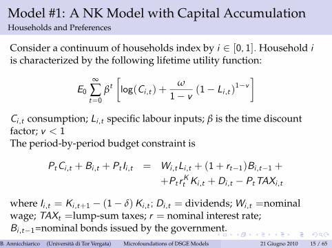
Model #1: A NK Model with Capital AccumulationHouseholds and Preferences
Consider a continuum of households index by i 2 [0, 1]. Household iis characterized by the following lifetime utility function:
E0∞
∑t=0
βt�log(Ci ,t ) +
ω
1� v (1� Li ,t )1�v�
Ci ,t consumption; Li ,t specific labour inputs; β is the time discountfactor; v < 1The period-by-period budget constraint is
PtCi ,t + Bi ,t + Pt Ii ,t = Wi ,tLi ,t + (1+ rt�1)Bi ,t�1 +
+Pt rKt Ki ,t +Di ,t � PtTAXi ,t
where Ii ,t = Ki ,t+1 � (1� δ)Ki ,t ; Di ,t = dividends; Wi ,t =nominalwage; TAXt =lump-sum taxes; r = nominal interest rate;Bi ,t�1=nominal bonds issued by the government.
B. Annicchiarico (Università di Tor Vergata) (Institute)Microfoundations of DSGE Models 21 Giugno 2010 15 / 65
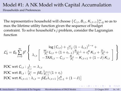
Model #1: A NK Model with Capital AccumulationHouseholds and Preferences
The representative household will choose fCi ,t ,Bi ,t ,Ki ,t+1g∞t=0 so as to
max the lifetime utility function given the sequence of budgetconstraint. To solve household’s j problem, consider the Lagrangianfunction
Li0 = E0∞
∑t=0
βt
8><>:log (Ci ,t ) + ω
1�v (1� Li ,t )1�v +
λi ,t
"W i ,tPtLi ,t + (1+ rt�1)
Bi ,t�1Pt
+ rKt Ki ,t +Di ,tPt+
�TAXi ,t � Ci ,t � Bi ,tPt�Ki ,t+1 + (1� δ)Ki ,t
# 9>=>;FOC wrt Ci ,t : 1
Ci ,t= λi ,t
FOC wrt Bi ,t : λi ,tPt= βEt
λi ,t+1Pt+1
(1+ rt )
FOC wrt Ki ,t+1 : λi ,t = βEtλi ,t+1�rKt+1 + (1� δ)
�B. Annicchiarico (Università di Tor Vergata) (Institute)Microfoundations of DSGE Models 21 Giugno 2010 16 / 65

Model #1: A NK Model with Capital AccumulationHouseholds and Preferences
Combining the previous conditions we derive the Euler equationgoverning the time path of consumption
1Ci ,t
= βEt1
Ci ,t+1
1+ rt1+ πt+1
and the asset equation according to which at the optimum a householdis indifferent between the two assets (capital and risk-free public debtbonds) since the expected benefit in terms of utility is the same:
Etλi ,t+11+ rt1+ πt+1
= Etλi ,t+1hrKt+1 + (1� δ)
i
B. Annicchiarico (Università di Tor Vergata) (Institute)Microfoundations of DSGE Models 21 Giugno 2010 17 / 65

Model #1: A NK Model with Capital AccumulationWage Setting
There is a continuum of unions each of which represents workers of acertain type. Effective labour input hired by the intermediate-goodfirm j is a CES function of the quantities of the different labour typesemployed:
Lt (j) =
1R0Li ,t (i)
σL�1σL di
! σLσL�1
where σL > 1 elasticity of substitution across different types of labourinputs. At the optimum (and under symmetry among firms) thedemand for each variety of labour input i is
Li ,t =�Wi ,t
Wt
��σL
Lt
where Wt =hR 10 W
1�σLi ,t di
i 11�σL such thatWtLt =
1R0Wi ,tLi ,tdi .
B. Annicchiarico (Università di Tor Vergata) (Institute)Microfoundations of DSGE Models 21 Giugno 2010 18 / 65

Model #1: A NK Model with Capital AccumulationWage Setting
The union representing worker of type i will setWi ,t in order to max
the expected utility of household i given Li ,t =�W i ,tWt
��σLLt . The
relevant part of the Lagrangian is
E0βt�
ω
1� v (1� Li ,t )1�v + λi ,t
Wi ,t
PtLi ,t
�At the optimum:
Wi ,t
Pt=
σLσL � 1| {z }
wage markup
ω (1� Li ,t )�v
λi ,t
B. Annicchiarico (Università di Tor Vergata) (Institute)Microfoundations of DSGE Models 21 Giugno 2010 19 / 65

Model #1: A NK Model with Capital AccumulationThe Government
The government budget constraint is
Bt = (1+ rt )Bt�1 + PtGt � PtTAXt
where Gt = G exp(εg ,t ) and εg ,t = ρg εg ,t + ξg ,t with ξg ,t � iid .N(0, σ2g ),while
PtTAXt = PtTAX + τPtBt
where τ is set in order to rule out any explosive path of the publicdebt ("passive" rule as meant by Leeper 1991).
B. Annicchiarico (Università di Tor Vergata) (Institute)Microfoundations of DSGE Models 21 Giugno 2010 20 / 65
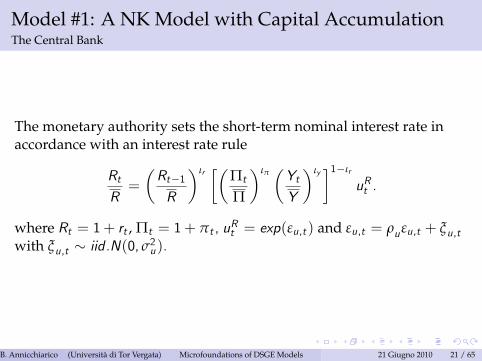
Model #1: A NK Model with Capital AccumulationThe Central Bank
The monetary authority sets the short-term nominal interest rate inaccordance with an interest rate rule
RtR=
�Rt�1R
�ιr ��Πt
Π
�ιπ �YtY
�ιy �1�ιr
uRt .
where Rt = 1+ rt , Πt = 1+ πt , uRt = exp(εu,t ) and εu,t = ρuεu,t + ξu,twith ξu,t � iid .N(0, σ2u).
B. Annicchiarico (Università di Tor Vergata) (Institute)Microfoundations of DSGE Models 21 Giugno 2010 21 / 65

Model #1: A NK Model with Capital AccumulationEquilibrium
Combining the above conditions, imposing symmetry between firms,households and unions the equilibrium of the economy is described bythe following equations.The Euler equation
λt = βEtλt+11+ rt1+ πt+1
The capital asset equation
λt = βEtλt+1hrKt+1 + (1� δ)
iThe Lagrange multiplier
λt =1Ct
The wage equation
Wt
Pt=
σLσL � 1
ω (1� Lt )�v
λt
B. Annicchiarico (Università di Tor Vergata) (Institute)Microfoundations of DSGE Models 21 Giugno 2010 22 / 65

Model #1: A NK Model with Capital AccumulationEquilibrium
The aggregate production function
Yt = AtLαtK
1�αt
The demand of capital
r kt = (1� α)MCtAtLαtK
�αt
The demand of labour
Wt
Pt= αMCtAtLα�1
t K 1�αt
The inflation equation
1� γp (Πt � 1)Πt + βγpEtλRt+1
λRt(Πt+1 � 1)
Yt+1Yt
Πt+1 = (1�MCt ) θ
B. Annicchiarico (Università di Tor Vergata) (Institute)Microfoundations of DSGE Models 21 Giugno 2010 23 / 65

Model #1: A NK Model with Capital AccumulationEquilibrium
The budget constraint of the government
Bt = (1+ rt )Bt�1 + PtGt � PtTAXt
The tax rulePtTAXt = PtTAX + τPtBt
The interest rate rule
RtR=
�Rt�1R
�ιr ��Πt
Π
�ιπ �YtY
�ιy �1�ιr
uRt .
B. Annicchiarico (Università di Tor Vergata) (Institute)Microfoundations of DSGE Models 21 Giugno 2010 24 / 65

Model #1: A NK Model with Capital AccumulationEquilibrium
The capital accumulation equation
Kt+1 = (1� δ)Kt + It
The resource constraint of the economy
Yt = Ct + It + Gt +γp2(Πt � 1)2 Yt
The exogenous processes governing At , Gt and uRt
B. Annicchiarico (Università di Tor Vergata) (Institute)Microfoundations of DSGE Models 21 Giugno 2010 25 / 65
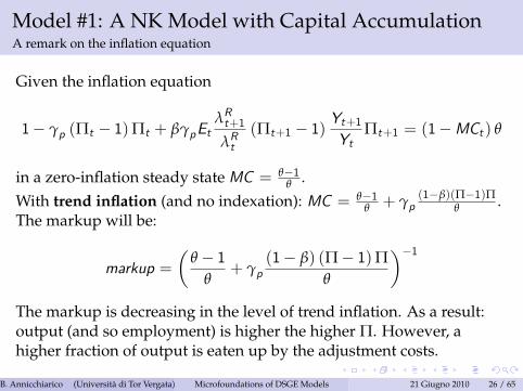
Model #1: A NK Model with Capital AccumulationA remark on the inflation equation
Given the inflation equation
1� γp (Πt � 1)Πt + βγpEtλRt+1
λRt(Πt+1 � 1)
Yt+1Yt
Πt+1 = (1�MCt ) θ
in a zero-inflation steady stateMC = θ�1θ .
With trend inflation (and no indexation): MC = θ�1θ + γp
(1�β)(Π�1)Πθ .
The markup will be:
markup =�
θ � 1θ
+ γp(1� β) (Π� 1)Π
θ
��1The markup is decreasing in the level of trend inflation. As a result:output (and so employment) is higher the higher Π. However, ahigher fraction of output is eaten up by the adjustment costs.
B. Annicchiarico (Università di Tor Vergata) (Institute)Microfoundations of DSGE Models 21 Giugno 2010 26 / 65

Model #1: A NK Model with Capital AccumulationCalibration
α = 2/3 labour shareβ = 0.99 discount factorδ = 0.1/4 depreciation ratev = 0.8 preference parameterγp = 58.25 degree of price rigidities 1� θ = 0.25θ = 6 elasticity of subst. between goodsσL = 5 elasticity of subst. between labour inputsρA = 0.9 persistence of tech shockρG = 0.9 persistence of the public spending shockρR = 0.9 persistence of monetary policy shock
B. Annicchiarico (Università di Tor Vergata) (Institute)Microfoundations of DSGE Models 21 Giugno 2010 27 / 65
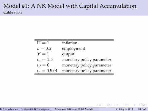
Model #1: A NK Model with Capital AccumulationCalibration
Π = 1 inflationL = 0.3 employmentY = 1 outputιπ = 1.5 monetary policy parameterιR = 0 monetary policy parameterιy = 0.5/4 monetary policy parameter
B. Annicchiarico (Università di Tor Vergata) (Institute)Microfoundations of DSGE Models 21 Giugno 2010 28 / 65
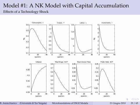
Model #1: A NK Model with Capital AccumulationEffects of a Technology Shock
0 20 400.1
0.2
0.3
0.4
0.5
0.6Consumption, c
quarters
%
0 20 400
0.2
0.4
0.6
0.8
1
1.2
1.4Output, Y
quarters0 20 40
0.2
0
0.2
0.4
0.6Labour, L
0 20 400.25
0.2
0.15
0.1
0.05
0Inflation
quarters
0 20 401
0
1
2
3
4
5
6Investments, I
quarters
%0 20 40
0.1
0.2
0.3
0.4
0.5
0.6
0.7
0.8Real Wage, W/P
quarters0 20 40
0.02
0.01
0
0.01
0.02
0.03
0.04
0.05Real Interest Rate
quarters0 20 40
0.1
0.05
0
0.05
0.1
0.15
0.2
0.25Public Debt, B/P
quarters
B. Annicchiarico (Università di Tor Vergata) (Institute)Microfoundations of DSGE Models 21 Giugno 2010 29 / 65

Model #1: A NK Model with Capital AccumulationEffects of a Technology Shock: Propagation
Higher Productivity ! lower marginal costs ! lower inflationAs in the basic RBC model a transitory productivity shock, whichtemporarily raises the real wage rate, increases employment(maybe we have a too low degree of price rigidity)Productivity " !MPK " !rental rate of capital "
Substitution effect increases savings (prevails)Consumption increases gradually (consumption smoothing)Investments increases on impact (the volatile component)As a result y increases more than proportionally.
B. Annicchiarico (Università di Tor Vergata) (Institute)Microfoundations of DSGE Models 21 Giugno 2010 30 / 65
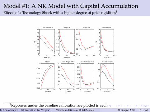
Model #1: A NK Model with Capital AccumulationEffects of a Technology Shock with a higher degree of price rigidities1
0 20 400
0.1
0.2
0.3
0.4
0.5
0.6
0.7Cons umption, c
quarters
%
0 20 400
0.2
0.4
0.6
0.8
1
1.2
1.4Output, Y
quarters0 20 40
0.4
0.2
0
0.2
0.4
0.6Labour, L
0 20 400.25
0.2
0.15
0.1
0.05
0Inflation
quarters
0 20 401
0
1
2
3
4
5
6Inv es tments , I
quarters
%
0 20 400
0.1
0.2
0.3
0.4
0.5
0.6
0.7Real Wage, W/P
quarters0 20 40
0.02
0.01
0
0.01
0.02
0.03
0.04
0.05Real Interes t Rate
quarters0 20 40
0.2
0.1
0
0.1
0.2Public Debt, B/P
quarters
1Reponses under the baseline calibration are plotted in red.B. Annicchiarico (Università di Tor Vergata) (Institute)Microfoundations of DSGE Models 21 Giugno 2010 31 / 65
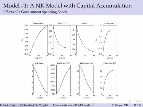
Model #1: A NK Model with Capital AccumulationEffects of a Government Spending Shock
0 20 400.08
0.07
0.06
0.05
0.04
0.03
0.02
0.01Consumption, c
quarters
%
0 20 400.02
0
0.02
0.04
0.06
0.08Output, Y
quarters0 20 40
0
0.02
0.04
0.06
0.08
0.1
0.12Labour, L
0 20 401
2
3
4
5
6x 10 3Inflation
quarters
0 20 400.4
0.3
0.2
0.1
0
0.1Investments, I
quarters
%0 20 40
0.04
0.035
0.03
0.025
0.02
0.015
0.01
0.005Real Wage, W/P
quarters0 20 40
0.5
1
1.5
2
2.5
3x 10 3Real Interest Rate
quarters0 20 40
0
0.2
0.4
0.6
0.8
1Public Debt, B/P
quarters
B. Annicchiarico (Università di Tor Vergata) (Institute)Microfoundations of DSGE Models 21 Giugno 2010 32 / 65

Model #1: A NK Model with Capital AccumulationEffects of a Government Spending Shock: Propagation
Government spending " !taxes increase " !net wage income#income effect (agents need to work more) !employment increasesthen gradually returns to normalconsumption falls, but the rise in government supply is temporary,hence agents respond by decreasing their capital holdings(consumption smoothing)firms will revise their prices upward (as real marginal costs arehigher)! the Central Bank will react to inflation by increasing thenominal interest rate more than proportionally ! as a result thereal interest rate will increase (lean against the wind policy).
As a result y will increase less than proportionally.Remark: no comovement between c and g .
B. Annicchiarico (Università di Tor Vergata) (Institute)Microfoundations of DSGE Models 21 Giugno 2010 33 / 65
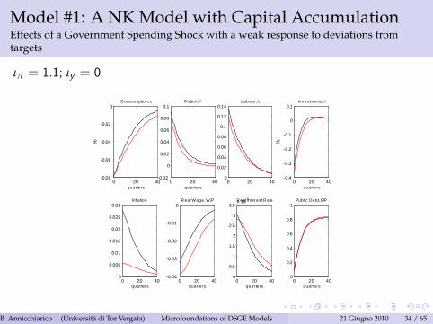
Model #1: A NK Model with Capital AccumulationEffects of a Government Spending Shock with a weak response to deviations fromtargets
ιπ = 1.1; ιy = 0
0 20 400.08
0.06
0.04
0.02
0Cons umption, c
quarters
%
0 20 400.02
0
0.02
0.04
0.06
0.08
0.1Output, Y
quarters0 20 40
0
0.02
0.04
0.06
0.08
0.1
0.12
0.14Labour, L
0 20 400
0.005
0.01
0.015
0.02
0.025
0.03Inflation
quarters
0 20 400.4
0.3
0.2
0.1
0
0.1Inv es tments , I
quarters
%0 20 40
0.04
0.03
0.02
0.01
0Real Wage, W/P
quarters0 20 40
0
0.5
1
1.5
2
2.5
3
3.5x 10³Real Interes t Rate
quarters0 20 40
0
0.2
0.4
0.6
0.8
1Public Debt, B/P
quarters
B. Annicchiarico (Università di Tor Vergata) (Institute)Microfoundations of DSGE Models 21 Giugno 2010 34 / 65
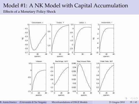
Model #1: A NK Model with Capital AccumulationEffects of a Monetary Policy Shock
0 20 400.7
0.6
0.5
0.4
0.3
0.2
0.1
0Consumption, c
quarters
%
0 20 402
1.5
1
0.5
0Output, Y
quarters0 20 40
3
2.5
2
1.5
1
0.5
0
0.5Labour, L
0 20 401.5
1
0.5
0
0.5Inflation
quarters
0 20 4010
8
6
4
2
0
2Investments, I
quarters
%0 20 40
1.4
1.2
1
0.8
0.6
0.4
0.2
0Real Wage, W/P
quarters0 20 40
0.01
0.015
0.02
0.025
0.03
0.035
0.04
0.045Real Interest Rate
quarters0 20 40
0
0.2
0.4
0.6
0.8
1
1.2
1.4Public Debt, B/P
quarters
B. Annicchiarico (Università di Tor Vergata) (Institute)Microfoundations of DSGE Models 21 Giugno 2010 35 / 65

Model #1: A NK Model with Capital AccumulationEffects of a Monetary Policy Shock: Propagation
The presence of price rigidities is a source of nontrivial real effects ofmonetary policy shocks.Firms cannot immediatly adjust the price of their good when theyreceive new information about costs or demand conditions.The shock generates an increase in the real rate, a decrease in inflation,output and employment.
B. Annicchiarico (Università di Tor Vergata) (Institute)Microfoundations of DSGE Models 21 Giugno 2010 36 / 65
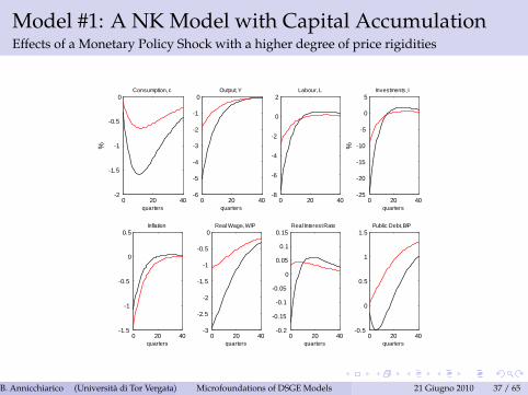
Model #1: A NK Model with Capital AccumulationEffects of a Monetary Policy Shock with a higher degree of price rigidities
0 20 402
1.5
1
0.5
0Consumption, c
quarters
%
0 20 406
5
4
3
2
1
0Output, Y
quarters0 20 40
8
6
4
2
0
2Labour, L
0 20 401.5
1
0.5
0
0.5Inflation
quarters
0 20 4025
20
15
10
5
0
5Investments, I
quarters
%0 20 40
3
2.5
2
1.5
1
0.5
0Real Wage, W/P
quarters0 20 40
0.2
0.15
0.1
0.05
0
0.05
0.1
0.15Real Interest Rate
quarters0 20 40
0.5
0
0.5
1
1.5Public Debt, B/P
quarters
B. Annicchiarico (Università di Tor Vergata) (Institute)Microfoundations of DSGE Models 21 Giugno 2010 37 / 65

Model #2: Model #1+ Habit+Adjust. Costs
Extend the previous model to account for:
external habit (see Lecture I)adjustment costs on investments (see Lecture I)adjustment costs on investments on labour (see Lecture I)
B. Annicchiarico (Università di Tor Vergata) (Institute)Microfoundations of DSGE Models 21 Giugno 2010 38 / 65

Model #2: Model #1+ Habit+Adjust. CostsHouseholds and Preferences
The typical household will solve the following problemHousehold i is characterized by the following lifetime utility function:
E0∞
∑t=0
βt�log(Ci ,t � heC t�1) +
ω
1� v (1� Li ,t )1�v�
C average aggregate consumption; he measure of habit intensityThe period-by-period budget constraint is
PtCi ,t + Bi ,t + Pt Ii ,t = Wi ,tLi ,t + (1+ rt�1)Bi ,t�1 + Pt rKt Ki ,t+Di ,t � PtTAXt � PtADJ(It ,Kt )
whereKi ,t+1 = (1� δ)Ki ,t + Ii ,t
ADJ(Ii ,t ,Ki ,t ) =γI2
�Ii ,tKi ,t
� δ
�2Ki ,t
B. Annicchiarico (Università di Tor Vergata) (Institute)Microfoundations of DSGE Models 21 Giugno 2010 39 / 65
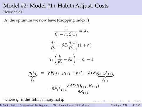
Model #2: Model #1+ Habit+Adjust. CostsHouseholds
At the optimum we now have (dropping index i )
1
Ct � heC t�1= λt
λtPt= βEt
λt+1Pt+1
(1+ rt )
γI
�ItKt� δK
�= qt � 1
qtλt|{z}ξt
= βEtλt+1rt+1 + β (1� δ)Etqt+1λt+1| {z }ξt+1
�βEtλt+1∂ADJ(It+1,Kt+1)
∂Kt+1
where qt is the Tobin’s marginal q.B. Annicchiarico (Università di Tor Vergata) (Institute)Microfoundations of DSGE Models 21 Giugno 2010 40 / 65

Model #2: Model #1+ Habit+Adjust. CostsIntermediate-goods firms the adjustment costs on labour
We now assume that hiring and firing unionized workers is costly, inparticular we have:
ADJ_Lt (j) =γL2
�Lt (j)Lt�1 (j)
� 1�2Yt
As a result the optimal demand of labor is
Wt
Pt= αLMCt (J)
Yt (j)Lt (j)
� γL
�Lt (j)Lt�1 (j)
� 1�
YtLt�1 (j)
+
+βγLEtλRt+1
λRt
�Lt+1 (j)Lt (j)
� 1�Lt+1 (j)
Lt (j)2 Yt+1
B. Annicchiarico (Università di Tor Vergata) (Institute)Microfoundations of DSGE Models 21 Giugno 2010 41 / 65

Model #2: Model #1+ Habit+Adjust. CostsThe resource constrain of the economy
The resource constraint of the economy is now
Yt = Ct + It + Gt +
+γp2(Πt � 1)2 Yt +
+γL2
�Lt (j)Lt�1 (j)
� 1�2Yt +
+γI2
�ItKt� δ
�2Kt
B. Annicchiarico (Università di Tor Vergata) (Institute)Microfoundations of DSGE Models 21 Giugno 2010 42 / 65
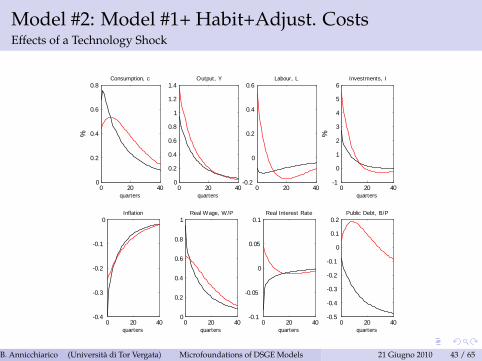
Model #2: Model #1+ Habit+Adjust. CostsEffects of a Technology Shock
0 20 400
0.2
0.4
0.6
0.8Consumption, c
quarters
%
0 20 400
0.2
0.4
0.6
0.8
1
1.2
1.4Output, Y
quarters0 20 40
0.2
0
0.2
0.4
0.6Labour, L
0 20 400.4
0.3
0.2
0.1
0Inflation
quarters
0 20 401
0
1
2
3
4
5
6Investments, I
quarters
%0 20 40
0
0.2
0.4
0.6
0.8
1Real Wage, W/P
quarters0 20 40
0.1
0.05
0
0.05
0.1Real Interest Rate
quarters0 20 40
0.5
0.4
0.3
0.2
0.1
0
0.1
0.2Public Debt, B/P
quarters
B. Annicchiarico (Università di Tor Vergata) (Institute)Microfoundations of DSGE Models 21 Giugno 2010 43 / 65
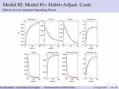
Model #2: Model #1+ Habit+Adjust. CostsEffects of a Government Spending Shock
0 20 400.14
0.12
0.1
0.08
0.06
0.04
0.02
0Consumption, c
quarters
%
0 20 400.02
0
0.02
0.04
0.06
0.08Output, Y
quarters0 20 40
0
0.02
0.04
0.06
0.08
0.1
0.12Labour, L
0 20 400
0.01
0.02
0.03
0.04
0.05
0.06Inflation
quarters
0 20 400.5
0.4
0.3
0.2
0.1
0
0.1
0.2Investments, I
quarters
%0 20 40
0.2
0.15
0.1
0.05
0Real Wage, W/P
quarters0 20 40
0
0.005
0.01
0.015
0.02
0.025
0.03Real Interest Rate
quarters0 20 40
0
0.2
0.4
0.6
0.8
1Public Debt, B/P
quarters
B. Annicchiarico (Università di Tor Vergata) (Institute)Microfoundations of DSGE Models 21 Giugno 2010 44 / 65
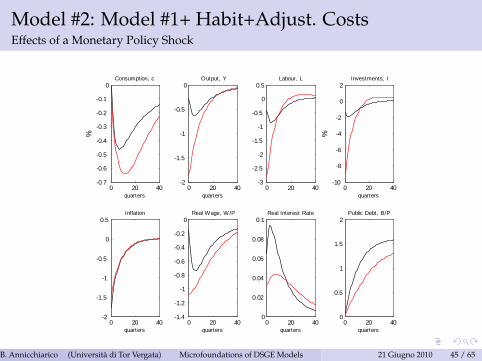
Model #2: Model #1+ Habit+Adjust. CostsEffects of a Monetary Policy Shock
0 20 400.7
0.6
0.5
0.4
0.3
0.2
0.1
0Consumption, c
quarters
%
0 20 402
1.5
1
0.5
0Output, Y
quarters0 20 40
3
2.5
2
1.5
1
0.5
0
0.5Labour, L
0 20 402
1.5
1
0.5
0
0.5Inflation
quarters
0 20 4010
8
6
4
2
0
2Investments, I
quarters
%0 20 40
1.4
1.2
1
0.8
0.6
0.4
0.2
0Real Wage, W/P
quarters0 20 40
0
0.02
0.04
0.06
0.08
0.1Real Interest Rate
quarters0 20 40
0
0.5
1
1.5
2Public Debt, B/P
quarters
B. Annicchiarico (Università di Tor Vergata) (Institute)Microfoundations of DSGE Models 21 Giugno 2010 45 / 65

Model #3: Model #1+RoT
Extend the Model #1 to account for:
Consider rule of thumb households as in Galí, López-Salido andVallés (2007).
B. Annicchiarico (Università di Tor Vergata) (Institute)Microfoundations of DSGE Models 21 Giugno 2010 46 / 65
Model #3: Model #1+RoTHouseholds
There is a continuum of households. Population is constant andnormalized to 1.A fraction sNR of households do not borrow and save, and justconsume their current labor income (hand-to-mouth households) !extreme form of non-Ricardian behaviorMotivation: an extensive empirical literature provides evidence of“excessive” dependence of consumption on current income; deviationsfrom the permanent income hypothesis.As a result now we have two types of households:
Non-Ricardian households (population share sNR )Ricardian households (population share 1� sNR )
B. Annicchiarico (Università di Tor Vergata) (Institute)Microfoundations of DSGE Models 21 Giugno 2010 47 / 65

Model #3: Model #1+RoTThe Ricardian Households
The typical Ricardian household will solve the following problemHousehold i is characterized by the following lifetime utility function:
E0∞
∑t=0
βt�log(CRi ,t � heC t�1) +
ω
1� v�1� LRi ,t
�1�v �C average aggregate consumption; he measure of habit intensityThe period-by-period budget constraint is
PtCRi ,t + Bri ,t + Pt I
ri ,t = Wi ,tLRi ,t + (1+ rt�1)B
Ri ,t�1 +
+Pt rKt KRi ,t +D
Ri ,t � PtTAXRt
whereKRi ,t+1 = (1� δ)KRi ,t + I
Ri ,t
B. Annicchiarico (Università di Tor Vergata) (Institute)Microfoundations of DSGE Models 21 Giugno 2010 48 / 65
Model #3: Model #1+RoTThe Ricardian Households
At the optimum we now have (dropping index i) we have thestandard optimality conditions:
1CRt
= λRt
λRtPt= βEt
λRt+1Pt+1
(1+ rt )
λi ,t = βEtλi ,t+1hrKt+1 + (1� δ)
i
B. Annicchiarico (Università di Tor Vergata) (Institute)Microfoundations of DSGE Models 21 Giugno 2010 49 / 65

Model #3: Model #1+RoTThe Non-Ricardian Households
Non-Ricardian households are assumed to behave in a“hand-to-mouth” fashion: they fully consume their current laborincome (no consumption smoothing).The representative household of this category derives utility fromconsumption and leisure:
logCNRi ,t �ω
1� v�1� LNRi ,t
�1�vNAgiven a flow budget constraint of the form:
PtCNRi ,t = Wi ,tLNRi ,t � PtTAXNRi ,t
Consumption function is then:
CNRi ,t =Wi ,t
PtLNRi ,t � TAXNRi ,t
B. Annicchiarico (Università di Tor Vergata) (Institute)Microfoundations of DSGE Models 21 Giugno 2010 50 / 65
Model #3: Model #1+RoTAggregate variables
Aggregate consumption is now defined as
Ct � sNRCNRt + (1� sNR )CRt
while investments and capital aggregates of the economy are give by
It � (1� sNR )IRt
Kt � (1� sNR )KRt
B. Annicchiarico (Università di Tor Vergata) (Institute)Microfoundations of DSGE Models 21 Giugno 2010 51 / 65
Model #3: Model #1+RoTWage Setting
New assumption: The fraction of Non-Ricardian and Ricardianhouseholds is uniformly distributed across workers types and henceacross unions. Each period a typical union representing worker i setsthe wage for its workers in order to maximize the objective function ofthe form
sNR
�ω
1� v (1� Li ,t )1�v + λNRi ,t
Wi ,t
PtLi ,t
�+
+(1� sNR )�
ω
1� v (1� Li ,t )1�v + λRi ,t
Wi ,t
PtLi ,t
�s.t. to the demand schedule: Li ,t =
�W i ,tWt
��σLLt . At the optimum the
wage equation is
σLσL � 1
ω (1� Lt )�v =hsNRλNRt + (1� sNR )λRt
i Wt
Pt
B. Annicchiarico (Università di Tor Vergata) (Institute)Microfoundations of DSGE Models 21 Giugno 2010 52 / 65

Model #3: Model #1+RoTThe government
The government budget constraint is
Bt = (1+ rt )Bt�1 + PtGt � PtTAXt
where Gt = G exp(εg ,t ) and εg ,t = ρg εg ,t + ξg ,t with ξg ,t � iid .N(0, σ2g ),while
TAXt � sNRTAXNRt + (1� sNR )TAXRtwhere we assume that TAXNRt = TAXRt = TAXtThe fiscal rule is as before:
PtTAXt = PtTAX + τPtBt
Set sNR = 0.20.
B. Annicchiarico (Università di Tor Vergata) (Institute)Microfoundations of DSGE Models 21 Giugno 2010 53 / 65
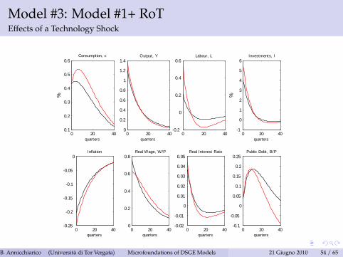
Model #3: Model #1+ RoTEffects of a Technology Shock
0 20 400.1
0.2
0.3
0.4
0.5
0.6Consumption, c
quarters
%
0 20 400
0.2
0.4
0.6
0.8
1
1.2
1.4Output, Y
quarters0 20 40
0.2
0
0.2
0.4
0.6Labour, L
0 20 400.25
0.2
0.15
0.1
0.05
0Inflation
quarters
0 20 401
0
1
2
3
4
5
6Investments, I
quarters
%0 20 40
0
0.2
0.4
0.6
0.8Real Wage, W/P
quarters0 20 40
0.02
0.01
0
0.01
0.02
0.03
0.04
0.05Real Interest Rate
quarters0 20 40
0.1
0.05
0
0.05
0.1
0.15
0.2
0.25Public Debt, B/P
quarters
B. Annicchiarico (Università di Tor Vergata) (Institute)Microfoundations of DSGE Models 21 Giugno 2010 54 / 65
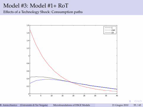
Model #3: Model #1+ RoTEffects of a Technology Shock: Consumption paths
0 5 10 15 20 25 30 35 400
0.2
0.4
0.6
0.8
1
1.2
1.4
1.6
1.8CCNRCR
B. Annicchiarico (Università di Tor Vergata) (Institute)Microfoundations of DSGE Models 21 Giugno 2010 55 / 65
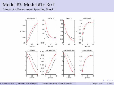
Model #3: Model #1+ RoTEffects of a Government Spending Shock
0 20 400.08
0.06
0.04
0.02
0Consumption, c
quarters
%
0 20 400.02
0
0.02
0.04
0.06
0.08Output, Y
quarters0 20 40
0
0.02
0.04
0.06
0.08
0.1
0.12Labour, L
0 20 401
2
3
4
5
6x 10 3Inflation
quarters
0 20 400.6
0.5
0.4
0.3
0.2
0.1
0
0.1Investments, I
quarters
%0 20 40
0.04
0.035
0.03
0.025
0.02
0.015
0.01
0.005Real Wage, W/P
quarters0 20 40
0.5
1
1.5
2
2.5
3x 10 3Real Interest Rate
quarters0 20 40
0
0.2
0.4
0.6
0.8
1Public Debt, B/P
quarters
B. Annicchiarico (Università di Tor Vergata) (Institute)Microfoundations of DSGE Models 21 Giugno 2010 56 / 65
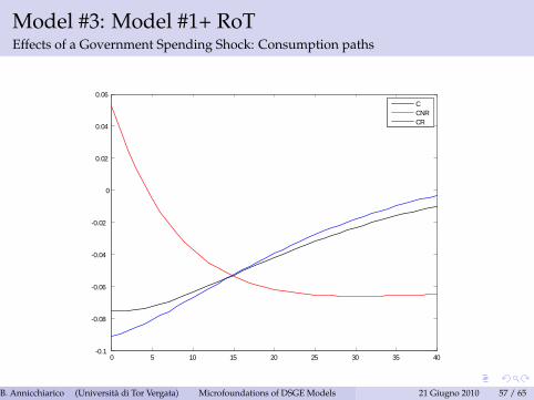
Model #3: Model #1+ RoTEffects of a Government Spending Shock: Consumption paths
0 5 10 15 20 25 30 35 400.1
0.08
0.06
0.04
0.02
0
0.02
0.04
0.06CCNRCR
B. Annicchiarico (Università di Tor Vergata) (Institute)Microfoundations of DSGE Models 21 Giugno 2010 57 / 65
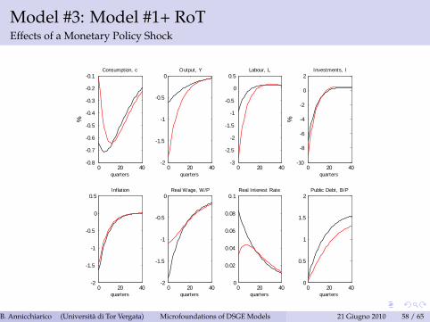
Model #3: Model #1+ RoTEffects of a Monetary Policy Shock
0 20 400.8
0.7
0.6
0.5
0.4
0.3
0.2
0.1Consumption, c
quarters
%
0 20 402
1.5
1
0.5
0Output, Y
quarters0 20 40
3
2.5
2
1.5
1
0.5
0
0.5Labour, L
0 20 402
1.5
1
0.5
0
0.5Inflation
quarters
0 20 4010
8
6
4
2
0
2Investments, I
quarters
%0 20 40
2
1.5
1
0.5
0Real Wage, W/P
quarters0 20 40
0
0.02
0.04
0.06
0.08
0.1Real Interest Rate
quarters0 20 40
0
0.5
1
1.5
2Public Debt, B/P
quarters
B. Annicchiarico (Università di Tor Vergata) (Institute)Microfoundations of DSGE Models 21 Giugno 2010 58 / 65
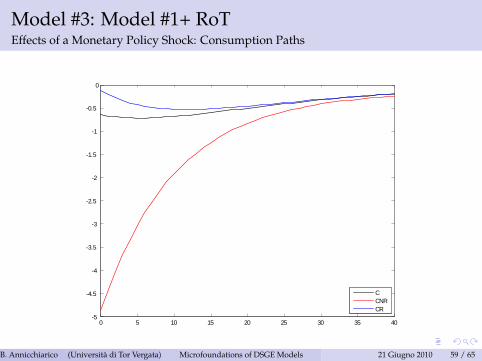
Model #3: Model #1+ RoTEffects of a Monetary Policy Shock: Consumption Paths
0 5 10 15 20 25 30 35 405
4.5
4
3.5
3
2.5
2
1.5
1
0.5
0
CCNRCR
B. Annicchiarico (Università di Tor Vergata) (Institute)Microfoundations of DSGE Models 21 Giugno 2010 59 / 65
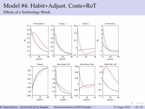
Model #4: Habit+Adjust. Costs+RoTEffects of a Technology Shock
0 20 400
0.1
0.2
0.3
0.4
0.5
0.6
0.7Consumption, c
quarters
%
0 20 400
0.2
0.4
0.6
0.8
1
1.2
1.4Output, Y
quarters0 20 40
0.2
0
0.2
0.4
0.6Labour, L
0 20 400.35
0.3
0.25
0.2
0.15
0.1
0.05
0Inflation
quarters
0 20 401
0
1
2
3
4
5
6Investments, I
quarters
%0 20 40
0
0.2
0.4
0.6
0.8
1
1.2
1.4Real Wage, W/P
quarters0 20 40
0.04
0.02
0
0.02
0.04
0.06Real Interest Rate
quarters0 20 40
0.3
0.2
0.1
0
0.1
0.2Public Debt, B/P
quarters
B. Annicchiarico (Università di Tor Vergata) (Institute)Microfoundations of DSGE Models 21 Giugno 2010 60 / 65
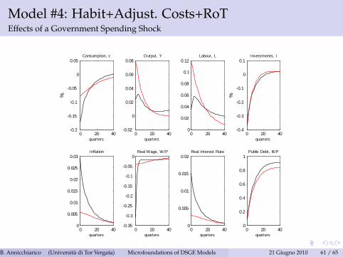
Model #4: Habit+Adjust. Costs+RoTEffects of a Government Spending Shock
0 20 400.2
0.15
0.1
0.05
0
0.05Consumption, c
quarters
%
0 20 400.02
0
0.02
0.04
0.06
0.08Output, Y
quarters0 20 40
0
0.02
0.04
0.06
0.08
0.1
0.12Labour, L
0 20 400
0.005
0.01
0.015
0.02
0.025
0.03Inflation
quarters
0 20 400.4
0.3
0.2
0.1
0
0.1Investments, I
quarters
%0 20 40
0.35
0.3
0.25
0.2
0.15
0.1
0.05
0Real Wage, W/P
quarters0 20 40
0
0.005
0.01
0.015
0.02Real Interest Rate
quarters0 20 40
0
0.2
0.4
0.6
0.8
1Public Debt, B/P
quarters
B. Annicchiarico (Università di Tor Vergata) (Institute)Microfoundations of DSGE Models 21 Giugno 2010 61 / 65
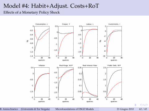
Model #4: Habit+Adjust. Costs+RoTEffects of a Monetary Policy Shock
0 20 401.4
1.2
1
0.8
0.6
0.4
0.2
0Consumption, c
quarters
%
0 20 402
1.5
1
0.5
0
0.5Output, Y
quarters0 20 40
3
2.5
2
1.5
1
0.5
0
0.5Labour, L
0 20 402
1.5
1
0.5
0
0.5Inflation
quarters
0 20 4010
8
6
4
2
0
2Investments, I
quarters
%0 20 40
3
2.5
2
1.5
1
0.5
0Real Wage, W/P
quarters0 20 40
0
0.05
0.1
0.15
0.2
0.25Real Interest Rate
quarters0 20 40
0
0.5
1
1.5
2
2.5Public Debt, B/P
quarters
B. Annicchiarico (Università di Tor Vergata) (Institute)Microfoundations of DSGE Models 21 Giugno 2010 62 / 65

DiscussionWhat is still missing to have a more complete model?
IndexationWage rigiditiesVariable capacity utilizationInternational trade and international capital markets
B. Annicchiarico (Università di Tor Vergata) (Institute)Microfoundations of DSGE Models 21 Giugno 2010 63 / 65

DiscussionChallenges of DSGE modelling
Labour migration and remittancesForeign direct investmentsHeterogenous workers (atypical, self-employed etc...)Informal sectorRole of relative price movementsNon-market sector (public goods)Financial market frictionsPortfolio choiceTerm structure of interest ratesCurrency risk premiaEndogenous growthTime varying parameters and structural breaksEstimation problems
B. Annicchiarico (Università di Tor Vergata) (Institute)Microfoundations of DSGE Models 21 Giugno 2010 64 / 65

References
Galí, J., López-Salido, J.D., Vallés, J., (2007), Understanding the Effects of GovernmentSpending on Consumption, Journal of the European Economic Association, 5(1).Rotemberg, J., (1983), Aggregate Consequences of Fixed Costs of Price Adjustment,American Economic Review, 73(3).Ascari, G., Merkl, C., (2009), Real Wage Rigidities and the Cost of Disinflations,Journal of Money, Credit and Banking, 41(2-3).Ascari, G., Ropele, T., (2007), Optimal monetary policy under low trend inflation,Journal of Monetary Economics, 54(8).Ascari, G., Rossi, L. (2009), Real Wage Rigidities and Disinflation Dynamics: Calvo vs.Rotemberg Pricing, University of Pavia.Ascari, G., Rossi, L. (2010), Trend Inflation, Non-linearities and Firms Price-Setting:Rotemberg vs. Calvo, University of Pavia.Leeper, E. M., (1991), Equilibria under ’active’ and ’passive’ monetary and fiscalpolicies, Journal of Monetary Economics 27(1).
B. Annicchiarico (Università di Tor Vergata) (Institute)Microfoundations of DSGE Models 21 Giugno 2010 65 / 65