Solution and Estimation Methods for DSGE Modelseconomics.sas.upenn.edu/~jesusfv/FVRS_Handbook.pdf · Solution and Estimation Methods for DSGE Models 531. DSGE model with recursive

CHAPTER 9

Solution and Estimation Methodsfor DSGE ModelsJ. Fernández-Villaverde*, J.F. Rubio-Ramírez†,{,§,¶, F. Schorfheide**University of Pennsylvania, Philadelphia, PA, United States†Emory University, Atlanta, GA, United States{Federal Reserve Bank of Atlanta, Atlanta, GA, United States§BBVA Research, Madrid, Madrid, Spain¶Fulcrum Asset Management, London, England, United Kingdom

Contents

1. Introduction 530Part I. Solving DSGE Models 531

2. Solution Methods for DSGE Models 5313. A General Framework 534

3.1 The Stochastic Neoclassical Growth Model 5343.2 A Value Function 5353.3 Euler Equation 5363.4 Conditional Expectations 5373.5 The Way Forward 539

4. Perturbation 5404.1 The Framework 5414.2 The General Case 543

4.2.1 Steady State 5434.2.2 Exogenous Stochastic Process 5464.2.3 Solution of the Model 5494.2.4 First-Order Perturbation 5514.2.5 Second-Order Perturbation 5574.2.6 Higher-Order Perturbations 559

4.3 A Worked-Out Example 5604.4 Pruning 5674.5 Change of Variables 568

4.5.1 A Simple Example 5694.5.2 A More General Case 5704.5.3 The Optimal Change of Variables 571

4.6 Perturbing the Value Function 5745. Projection 577

5.1 A Basic Projection Algorithm 5795.2 Choice of Basis and Metric Functions 5835.3 Spectral Bases 583

5.3.1 Unidimensional Bases 5845.3.2 Multidimensional Bases 592

5.4 Finite Elements 598

527Handbook of Macroeconomics, Volume 2A © 2016 Elsevier B.V.ISSN 1574-0048, http://dx.doi.org/10.1016/bs.hesmac.2016.03.006 All rights reserved.

http://dx.doi.org/10.1016/bs.hesmac.2016.03.006

5.5 Objective Functions 6035.5.1 Weight Function I: Least Squares 6045.5.2 Weight Function II: Subdomain 6055.5.3 Weight Function III: Collocation 6055.5.4 Weight Function IV: Galerkin or Rayleigh–Ritz 605

5.6 A Worked-Out Example 6075.7 Smolyak's Algorithm 611

5.7.1 Implementing Smolyak's Algorithm 6125.7.2 Extensions 618

6. Comparison of Perturbation and Projection Methods 6197. Error Analysis 620

7.1 A w2 Accuracy Test 6217.2 Euler Equation Errors 6227.3 Improving the Error 626

Part II. Estimating DSGE Models 6278. Confronting DSGE Models with Data 627

8.1 A Stylized DSGE Model 6288.1.1 Loglinearized Equilibrium Conditions 6298.1.2 Model Solution 6308.1.3 State-Space Representation 632

8.2 Model Implications 6338.2.1 Autocovariances and Forecast Error Variances 6358.2.2 Spectrum 6388.2.3 Impulse Response Functions 6408.2.4 Conditional Moment Restrictions 6418.2.5 Analytical Calculation of Moments vs Simulation Approximations 642

8.3 Empirical Analogs 6438.3.1 Autocovariances 6438.3.2 Spectrum 6458.3.3 Impulse Response Functions 6468.3.4 Conditional Moment Restrictions 648

8.4 Dealing with Trends 6499. Statistical Inference 650

9.1 Identification 6529.1.1 Local Identification 6529.1.2 Global Identification 655

9.2 Frequentist Inference 6569.2.1 “Correct” Specification of DSGE Model 6569.2.2 Misspecification and Incompleteness of DSGE Models 657

9.3 Bayesian Inference 6589.3.1 “Correct” Specification of DSGE Models 6599.3.2 Misspecification of DSGE Models 660

10. The Likelihood Function 66210.1 A Generic Filter 66310.2 Likelihood Function for a Linearized DSGE Model 66310.3 Likelihood Function for Nonlinear DSGE Models 666

10.3.1 Generic Particle Filter 66710.3.2 Bootstrap Particle Filter 669

528 Handbook of Macroeconomics

10.3.3 (Approximately) Conditionally Optimal Particle Filter 67111. Frequentist Estimation Techniques 672

11.1 Likelihood-Based Estimation 67311.1.1 Textbook Analysis of the ML Estimator 67311.1.2 Illustration 67511.1.3 Stochastic Singularity 67611.1.4 Dealing with Lack of Identification 677

11.2 (Simulated) Minimum Distance Estimation 67811.2.1 Textbook Analysis 67911.2.2 Approximating Model-Implied Moments 68111.2.3 Misspecification 68211.2.4 Illustration 68411.2.5 Laplace Type Estimators 685

11.3 Impulse Response Function Matching 68611.3.1 Invertibility and Finite-Order VAR Approximations 68611.3.2 Practical Considerations 68711.3.3 Illustration 688

11.4 GMM Estimation 69112. Bayesian Estimation Techniques 693

12.1 Prior Distributions 69412.2 Metropolis–Hastings Algorithm 695

12.2.1 The Basic MH Algorithm 69712.2.2 Random-Walk Metropolis–Hastings Algorithm 69712.2.3 Numerical Illustration 69812.2.4 Blocking 70012.2.5 Marginal Likelihood Approximations 70112.2.6 Extensions 70212.2.7 Particle MCMC 702

12.3 SMC Methods 70312.3.1 The SMC Algorithm 70412.3.2 Tuning the SMC Algorithm 70612.3.3 Numerical Illustration 707

12.4 Model Diagnostics 70812.5 Limited Information Bayesian Inference 709

12.5.1 Single-Equation Estimation 70912.5.2 Inverting a Sampling Distribution 70912.5.3 Limited-Information Likelihood Functions 71112.5.4 Nonparametric Likelihood Functions 712

13. Conclusion 712Acknowledgments 713References 713

Abstract

This chapter provides an overview of solution and estimation techniques for dynamic stochasticgeneral equilibrium models. We cover the foundations of numerical approximation techniques as wellas statistical inference and survey the latest developments in the field.

529Solution and Estimation Methods for DSGE Models

Keywords

Approximation error analysis, Bayesian inference, DSGE model, Frequentist inference, GMM estimation,Impulse response function matching, Likelihood-based inference, Metropolis-Hastings algorithm,Minimum distance estimation, Particle filter, Perturbation methods, Projection methods, SequentialMonte Carlo.

JEL Classification Codes

C11, C13, C32, C52, C61, C63, E32, E52

1. INTRODUCTION

The goal of this chapter is to provide an illustrative overview of the state-of-the-art

solution and estimation methods for dynamic stochastic general equilibrium (DSGE)

models. DSGE models use modern macroeconomic theory to explain and predict

comovements of aggregate time series over the business cycle. The term DSGE model

encompasses a broad class of macroeconomic models that spans the standard neoclassical

growth model discussed in King et al. (1988) as well as New Keynesian monetary models

with numerous real and nominal frictions along the lines of Christiano et al. (2005) and

Smets and Wouters (2003). A common feature of these models is that decision rules of

economic agents are derived from assumptions about preferences, technologies, informa-

tion, and the prevailing fiscal and monetary policy regime by solving intertemporal opti-

mization problems. As a consequence, the DSGE model paradigm delivers empirical

models with a strong degree of theoretical coherence that are attractive as a laboratory

for policy experiments. Modern DSGE models are flexible enough to accurately

track and forecast macroeconomic time series fairly well. They have become one of

the workhorses of monetary policy analysis in central banks.

The combination of solution and estimation methods in a single chapter reflects our

view of the central role of the tight integration of theory and data in macroeconomics.

Numerical solution methods allow us to handle the rich DSGE models that are needed

for business cycle analysis, policy analysis, and forecasting. Estimation methods enable

us to take these models to the data in a rigorous manner. DSGE model solution and

estimation techniques are the two pillars that form the basis for understanding the behav-

ior of aggregate variables such as GDP, employment, inflation, and interest rates, using

the tools of modern macroeconomics.

Unfortunately for PhD students and fortunately for those who have worked with

DSGE models for a long time, the barriers to entry into the DSGE literature are quite

high. The solution of DSGE models demands familiarity with numerical approximation

techniques and the estimation of the models is nonstandard for a variety of reasons,

including a state-space representation that requires the use of sophisticated filtering tech-

niques to evaluate the likelihood function, a likelihood function that depends in a


complicated way on the underlying model parameters, and potential model misspecifica-

tion that renders traditional econometric techniques based on the “axiom of correct

specification” inappropriate. The goal of this chapter is to lower the barriers to entry into

this field by providing an overview of what have become the “standard” methods of

solving and estimating DSGEmodels in the past decade and by surveying the most recent

technical developments. The chapter focuses on methods more than substantive appli-

cations, though we provide detailed numerical illustrations as well as references to applied

research. The material is grouped into two parts. Part I: Solving DSGE Models

(Sections 2–7) is devoted to solution techniques, which are divided into perturbation

and projection techniques. Part II: Estimating DSGE Models (Sections 8–12) focuses

on estimation. We cover both Bayesian and frequentist estimation and inference

techniques.

PART I. SOLVING DSGE MODELS2. SOLUTION METHODS FOR DSGE MODELS

DSGE models do not admit, except in a few cases, a closed-form solution to their equi-

librium dynamics that we can derive with “paper and pencil.” Instead, we have to resort

to numerical methods and a computer to find an approximated solution.

However, numerical analysis and computer programming are not a part of the stan-

dard curriculum for economists at either the undergraduate or the graduate level. This

educational gap has created three problems. The first problem is that many macroeco-

nomists have been reluctant to accept the limits imposed by analytic results. The cavalier

assumptions that are sometimes taken to allow for closed-form solutions may confuse

more than clarify. While there is an important role for analytic results for building intu-

ition, for understanding economic mechanisms, and for testing numerical approxima-

tions, many of the questions that DSGE models are designed to address require a

quantitative answer that only numerical methods can provide. Think, for example, about

the optimal response of monetary policy to a negative supply shock. Suggesting that the

monetary authority should lower the nominal interest rate to smooth output is not

enough for real-world advice. We need to gauge the magnitude and the duration of such

an interest rate reduction. Similarly, showing that an increase in government spending

raises output does not provide enough information to design an effective countercyclical

fiscal package.

The second problem is that the lack of familiarity with numerical analysis has led to

the slow diffusion of best practices in solution methods and little interest in issues such as

the assessment of numerical errors. Unfortunately, the consequences of poor approxima-

tions can be severe. Kim and Kim (2003) document how inaccurate solutions may cause

spurious welfare reversals. Similarly, the identification of parameter values may depend

on the approximated solution. For instance, van Binsbergen et al. (2012) show that a


DSGE model with recursive preferences needs to be solved with higher-order approx-

imations for all parameters of interest to be identified. Although much progress in the

quality of computational work has been made in the last few years, there is still room

for improvement. This is particularly important as essential nonlinearities—such as those

triggered by nonstandard utility functions, time-varying volatility, or occasionally binding

constraints—are becoming central to much research on the frontier of macroeconomics.

Nonstandard utility functions such as the very popular Epstein–Zin preferences (Epstein

and Zin, 1989) are employed in DSGE models by Tallarini (2000), Piazzesi and

Schneider (2006), Rudebusch and Swanson (2011, 2012), van Binsbergen et al.

(2012), and Fernandez-Villaverde et al. (2014), among many others. DSGE models with

time-varying volatility include Fernandez-Villaverde and Rubio-Ramırez (2007),

Justiniano and Primiceri (2008), Bloom (2009), Fernandez-Villaverde et al. (2011,

2015b), also among many others. Occasionally binding constraints can be caused by

many different mechanisms. Two popular ones are the zero lower bound (ZLB) of

nominal interest rates (Eggertsson and Woodford, 2003; Christiano et al., 2011;

Fernandez-Villaverde et al., 2015a; Aruoba and Schorfheide, 2015; and Gust et al.,

2016) and financial frictions (such as in Bernanke and Gertler, 1989; Carlstrom and

Fuerst, 1997; Bernanke et al., 1999; Fernandez-Villaverde, 2010; Christiano et al.,

2014; and dozens of others). Inherent nonlinearities force macroeconomists to move

beyond traditional linearization methods.

The third problem is that, even within the set of state-of-the-art solution methods,

researchers have sometimes been unsure about the trade-offs (for example, regarding

speed vs accuracy) involved in choosing among different algorithms.

Part I of the chapter covers some basic ideas about solution methods for DSGE

models, discusses the trade-offs created by alternative algorithms, and introduces basic

concepts related to the assessment of the accuracy of the solution. Throughout the

chapter, we will include remarks with additional material for those readers willing to

dig deeper into technical details.

Because of space considerations, there are important topics we cannot cover in what

is already a lengthy chapter. First, we will not deal with value and policy function iter-

ation. Rust (1996) and Cai and Judd (2014) review numerical dynamic programming in

detail. Second, we will not discuss models with heterogeneous agents, a task already

well accomplished by Algan et al. (2014) and Nishiyama and Smetters (2014) (the for-

mer centering on models in the Krusell and Smith (1998) tradition and the latter focus-

ing on overlapping generations models). Although heterogeneous agent models are,

indeed, DSGE models, they are often treated separately for simplicity. For the purpose

of this chapter, a careful presentation of issues raised by heterogeneity will consume

many pages. Suffice it to say, nevertheless, that most of the ideas in our chapter can

also be applied, with suitable modifications, to models with heterogeneous agents.

Third, we will not spend much time explaining the peculiarities of Markov-switching


regime models and models with stochastic volatility. Finally, we will not explore how

the massively parallel programming allowed by graphic processor units (GPUs) is a

game-changer that opens the door to the solution of a much richer class of models.

See, for example, Aldrich et al. (2011) and Aldrich (2014). Finally, for general back-

ground, the reader may want to consult a good numerical analysis book for economists.

Judd (1998) is still the classic reference.

Two additional topics—a survey of the evolution of solution methods over time and

the contrast between the solution of models written in discrete and continuous time—are

briefly addressed in the next two remarks.

Remark 1 (The evolution of solution methods) Wewill skip a detailed historical survey of

methods employed for the solution of DSGE models (or more precisely, for their ances-

tors during the first two decades of the rational expectations revolution). Instead, we will

just mention four of the most influential approaches.

Fair and Taylor (1983) presented an extended path algorithm. The idea was to solve,

for a terminal date sufficiently far into the future, the path of endogenous variables using a

shooting algorithm. Recently, Maliar et al. (2015) have proposed a promising derivation

of this idea, the extended function path (EFP), to analyze applications that do not admit

stationary Markov equilibria.

Kydland and Prescott (1982) exploited the fact that the economy they were analyzing

was Pareto optimal to solve the social planner’s problem instead of the recursive equilib-

rium of their model. To do so, they substituted a linear quadratic approximation to the

original social planner’s problem and exploited the fast solution algorithms existing for

that class of optimization problems. We will discuss this approach and its relation with

perturbation in Remark 13.

King, Plosser, and Rebelo (in the widely disseminated technical appendix, not pub-

lished until 2002), building on Blanchard and Kahn (1980)’s approach, linearized the

equilibrium conditions of the model (optimality conditions, market clearing conditions,

etc.), and solved the resulting system of stochastic linear difference equations. We will

revisit linearization below by interpreting it as a first-order perturbation.

Christiano (1990) applied value function iteration to the social planner’s problem of a

stochastic neoclassical growth model.

Remark 2 (Discrete vs continuous time) In this chapter, we will deal with DSGE models

expressed in discrete time.We will only make passing references to models in continuous

time. We do so because most of the DSGE literature is in discrete time. This, however,

should not be a reason to forget about the recent advances in the computation of DSGE

models in continuous time (see Parra-Alvarez, 2015) or to underestimate the analytic

power of continuous time. Researchers should be open to both specifications and

opt, in each particular application, for the time structure that maximizes their ability

to analyze the model and take it to the data successfully.


3. A GENERAL FRAMEWORK

A large number of solution methods have been proposed to solve DSGE models. It is,

therefore, useful to have a general notation to express the model and its solution. This

general notation will make the similarities and differences among the solution methods

clear and will help us to link the different approaches with mathematics, in particular with

the well-developed study of functional equations.

Indeed, we can cast numerous problems in economics in the form of a functional

equation.a Let us define a functional equation more precisely. Let J1 and J2 be two func-

tional spaces,Ω�n (whereΩ is the state space), andH : J1! J2 be an operator between

these two spaces. A functional equation problem is to find a function d� J1: Ω!m

such that:

H dð Þ¼ 0: (1)

From Eq. (1), we can see that regular equations are nothing but particular examples of

functional equations. Also, note that 0 is the space zero, different in general than the zero

in the real numbers.

Examples of problems in macroeconomics that can be framed as a functional equation

include value functions, Euler equations, and conditional expectations. To make this

connection explicit, we introduce first the stochastic neoclassical growth model, the

ancestor of all modern DSGE models. Second, we show how we can derive a functional

equation problem that solves for the equilibrium dynamics of the model in terms of either

a value function, an Euler equation, or a conditional expectation. After this example, the

reader will be able to extend the steps in our derivations to her application.

3.1 The Stochastic Neoclassical Growth ModelWe have an economy with a representative household that picks a sequence of consump-

tion ct and capital kt to solve

maxct,kt +1f g

0

X∞t¼0

βtu ctð Þ (2)

where t is the conditional expectation operator evaluated at period t, β is the discount

factor, and u is the period utility function. For simplicity, we have eliminated the labor

supply decision.

a Much of we have to say in this chapter is not, by any means, limited to macroeconomics. Similar problems

appear in fields such as finance, industrial organization, international finance, etc.


The resource constraint of the economy is given by

ct + kt+1¼ ezt kαt + ð1�δÞkt (3)

where δ is the depreciation rate and zt is an AR(1) productivity process:

zt ¼ ρzt�1 + σεt,εt �Nð0,1Þ and ρj j< 1: (4)

Since both fundamental welfare theorems hold in this economy, we can jump between

the social planner’s problem and the competitive equilibrium according to which

approach is more convenient in each moment. In general, this would not be possible,

and some care is required to stay on either the equilibrium problem or the social planner’s

problem according to the goals of the exercise.

3.2 A Value FunctionUnder standard technical conditions (Stokey et al., 1989), we can transform the sequen-

tial problem defined by Eqs. (2)–(4) into a recursive problem in terms of a value function

V kt,ztð Þ for the social planner that depends on the two state variables of the economy,

capital, kt, and productivity, zt. More concretely, V kt,ztð Þ is defined by the Bellman

operator:

V kt,ztð Þ¼ maxkt +1

u eztkαt + ð1�δÞkt�kt+1

� �+ βtV kt+1,zt+1ð Þ� �

(5)

where we have used the resource constraint (3) to substitute for ct in the utility function

and the expectation in (5) is takenwith respect to (4). This value function has an associated

decision rule g :+�!+:

kt+1¼ g kt,ztð Þthat maps the states kt and zt into optimal choices of kt+1 (and, therefore, optimal choices

of ct ¼ ezt kαt + ð1�δÞkt� g kt,ztð Þ).Expressing the model as a value function problem is convenient for several reasons.

First, we have many results about the properties of value functions and the decision rules

associated with them (for example, regarding their differentiability). These results can be

put to good use both in the economic analysis of the problem and in the design of numer-

ical methods. The second reason is that, as a default, we can use value function iteration

(as explained in Rust, 1996 and Cai and Judd, 2014), a solutionmethod that is particularly

reliable, although often slow.

We can rewrite the Bellman operator as:

V kt,ztð Þ�maxkt +1

u eztkαt + ð1�δÞkt�kt+1

� �+ βtV kt+1,zt+1ð Þ� �¼ 0,


for all kt and zt. If we define:

H dð Þ¼V kt,ztð Þ�maxkt+1

u ezt kαt + ð1�δÞkt�kt+1

� �+ βtV kt+1,zt+1ð Þ� �¼ 0, (6)

for all kt and zt, where d � , �ð Þ¼V � , �ð Þ, we see how the operator H, a rewrite of the

Bellman operator, takes the value function V � , �ð Þ and obtains a zero. More precisely,

Eq. (6) is an integral equation given the presence of the expectation operator. This can

lead to some nontrivial measure theory considerations that we leave aside.

3.3 Euler EquationWe have outlined several reasons why casting the problem in terms of a value function is

attractive. Unfortunately, this formulation can be difficult. If the model does not satisfy

the two fundamental welfare theorems, we cannot easily move between the social plan-

ner’s problem and the competitive equilibrium. In that case, also, the value function of

the household and firms will require laws of motion for individual and aggregate state

variables that can be challenging to characterize.b

An alternative is to work directly with the set of equilibrium conditions of the model.

These include the first-order conditions for households, firms, and, if specified, govern-

ment, budget and resource constraints, market clearing conditions, and laws of motion

for exogenous processes. Since, at the core of these equilibrium conditions, we will have

the Euler equations for the agents in the model that encode optimal behavior (with the

other conditions being somewhat mechanical), this approach is commonly known as the

Euler equation method (sometimes also referred to as solving the equilibrium conditions

of the models). This solution strategy is extremely general and it allows us to handle

non-Pareto efficient economies without further complications.

In the case of the stochastic neoclassical growth model, the Euler equation for the

sequential problem defined by Eqs. (2)–(4) is:

u0 ctð Þ¼ βt u0 ct+1ð Þ αezt +1kα�1

t+1 + 1�δ� ��

: (7)

Again, under standard technical conditions, there is a decision rule g :+�!2+ for

the social planner that gives the optimal choice of consumption (g1 kt,ztð Þ) and capital

tomorrow (g2 kt,ztð Þ) given capital, kt, and productivity, zt, today. Then, we can rewrite

the first-order condition as:

u0 g1 kt,ztð Þ� �¼ βt u0 g1 g2 kt,ztð Þ,zt+1

� �� αeρzt + σεt+1 g2 kt ,ztð Þ� �α�1

+ 1�δ� �h i

,

b See Hansen and Prescott (1995), for examples of how to recast a non-Pareto optimal economy into the

mold of an associated Pareto-optimal problem.


for all kt and zt, where we have used the law of motion for productivity (4) to substitute

forzt+1 or, alternatively:

u0 g1 kt,ztð Þ� ��βt u0 g1 g2 kt,ztð Þ,zt+1


+ 1�δ� �h i !

¼ 0, (8)

for all kt and zt (note the composition of functions g1 g2 kt,ztð Þ,zt+1

� �when evaluating

consumption at t + 1). We also have the resource constraint:

g1 kt,ztð Þ+ g2 kt,ztð Þ¼ ezt kαt + ð1�δÞkt (9)

Then, we have a functional equation where the unknown object is the decision rule g.

Mapping Eqs. (8) and (9) into our operator H is straightforward:

H dð Þ¼u0 g1 kt,ztð Þ� �

�βt u0 g1 g2 kt,ztð Þ,zt+1


+ 1�δ� �h i

g1 kt,ztð Þ+ g2 kt,ztð Þ� ezt kαt �ð1�δÞkt¼ 0

8><>: ,

for all kt and zt, where d ¼ g.

In this simple model, we could also have substituted the resource constraint in Eq. (8)

and solved for a one-dimensional decision rule, but by leaving Eqs. (8) and (9), we illus-

trate how to handle cases where this substitution is either infeasible or inadvisable.

An additional consideration that we need to take care of is that the Euler equation (7)

is only a necessary condition. Thus, after finding g � , �ð Þ, we would also need to ensure

that a transversality condition of the form:

limt!∞

βtu0 ctð Þu0 c0ð Þkt ¼ 0

(or a related one) is satisfied. We will describe below how we build our solution methods

to ensure that this is, indeed, the case.

3.4 Conditional ExpectationsWe have a considerable degree of flexibility in how we specifyH and d. For instance, if

we go back to the Euler equation (7):

u0 ctð Þ¼ βt u0 ct+1ð Þ αezt+1kα�1

t+1 + 1�δ� ��

we may want to find the unknown conditional expectation:

t u0 ct+1ð Þ αezt+1kα�1

t+1 + 1�δ� ��

:

This may be the case either because the conditional expectation is the object of interest in

the analysis or because solving for the conditional expectation avoids problems associated


with the decision rule. For example, we could enrich the stochastic neoclassical growth

model with additional constraints (such as a nonnegative investment: kt+1 � (1 � δ)kt)that induce kinks or other undesirable properties in the decision rules. Even when those

features appear, the conditional expectation (since it smooths over different realizations of

the productivity shock) may still have properties such as differentiability that the

researcher can successfully exploit either in her numerical solution or later in the

economic analysis.c

To see how this would work, we can define g :+�!+:

g kt,ztð Þ¼t u0 ct+1ð Þ αezt+1kα�1

t+1 + 1�δ� ��

(10)

where we take advantage of t being a function of the states of the economy. Going

back to our the Euler equation (7) and the resource constraint (3), if we have access

to g, we can find:

ct ¼ u0 βg kt ,ztð Þð Þ�1 (11)

and

kt+1¼ ezt kαt + ð1�δÞkt�u0 βg kt ,ztð Þð Þ�1:

Thus, knowledge of the conditional expectation allows us to recover all the other

endogenous variables of interest in the model. To save on notation, we write ct ¼ cg,tand kt+1 ¼ kg,t to denote the values of ct and kt+1 implied by g. Similarly:

ct+1¼ cg, t+1¼ u0 βg kt+1,zt+1ð Þð Þ�1¼ u0 βg kg, t ,zt+1

� �� 1

is the value of ct+1 implied by the recursive application of g.

To solve for g, we use its definition in Eq. (10):

g kt,ztð Þ¼ βt u0 cg, t+1

� �αeρzt + σεt+1kα�1

g, t +1�δ� �h i

and write:

H dð Þ¼ g kt,ztð Þ�βt u0 cg, t+1

� �αeρzt + σεt+1kα�1

g, t +1�δ� �h i

¼ 0

where d ¼ g.

c See Fernandez-Villaverde et al. (2015a) for an example. The paper is interested in solving a NewKeynesian

business cycle model with a zero lower bound (ZLB) on the nominal interest rate. This ZLB creates a kink

on the function that maps states of the model into nominal interest rates. The paper gets around this prob-

lem by solving for consumption, inflation, and an auxiliary variable that encodes information similar to that

of a conditional expectation. Once these functions have been found, the rest of the endogenous variables

of the model, including the nominal interest rate, can be derived without additional approximations.

In particular, the ZLB is always satisfied.


3.5 The Way ForwardWe have argued that a large number of problems in macroeconomics can be expressed in

terms of a functional equation problem

H dð Þ¼ 0

and we have illustrated our assertion by building the operatorH for a value function, for

an Euler equation problem, and for a conditional expectation problem. Our examples,

though, do not constitute an exhaustive list. Dozens of other cases can be constructed

following the same ideas.

We will move now to study the two main families of solution methods for functional

equation problems: perturbation and projection methods. Both families replace the

unknown function d for an approximation dj x,θð Þ in terms of the state variables of the

model x and a vector of coefficients θ and a degree of approximation j (we are deliberately

being ambiguous about the interpretation of that degree). We will use the terminology

“parameters” to refer to objects describing the preferences, technology, and information

sets of the model. The discount factor, risk aversion, the depreciation rate, or the per-

sistence of the productivity shock are examples of parameters. We will call the numerical

terms “coefficients” in the numerical solution. While the “parameters” usually have a

clear economic interpretation associated with them, the “coefficients” will, most of

the time, lack such interpretation.

Remark 3 (Structural parameters?) We are carefully avoiding the adjective

“structural” when we discuss the parameters of the model. Here we follow

Hurwicz (1962), who defined a “structural parameter” as a parameter that was

invariant to a class of policy interventions the researcher is interested in analyzing.

Many parameters of interest may not be “structural” in Hurwicz’s sense. For exam-

ple, the persistence of a technology shock may depend on the barriers to entry/exit

in the goods and services industries and how quickly technological innovations can

diffuse. These barriers may change with variations in competition policy. See a

more detailed discussion on the “structural” character of parameters in DSGE

models as well as empirical evidence in Fernandez-Villaverde and Rubio-

Ramırez (2008).

The states of the model will be determined by the structure of the model. Even if, in the

words of Thomas Sargent, “finding the states is an art” (meaning both that there is no

constructive algorithm to do so and that the researcher may be able to find different sets

of states that accomplish the goal of fully describing the situation of the model, some of

which may be more useful than the others in one context but less so in another one),

determining the states is a step previous to the numerical solution of the model and,

therefore, outside the purview of this chapter.


4. PERTURBATION

Perturbation methods build approximate solutions to a DSGE economy by starting from

the exact solution of a particular case of the model or from the solution of a nearby model

whose solution we have access to. Perturbation methods are also known as asymptotic

methods, although we will avoid such a name because it risks confusion with related

techniques regarding the large sample properties of estimators as the ones we will intro-

duce in Part II of the chapter. In their more common incarnation in macroeconomics,

perturbation algorithms build Taylor series approximations to the solution of a DSGE

model around its deterministic steady state using implicit-function theorems. However,

other perturbation approaches are possible, and we should always talk about a perturbation

of the model instead of the perturbation. With a long tradition in physics and other natural

sciences, perturbation theory was popularized in economics by Judd and Guu (1993) and it

has been authoritatively presented by Judd (1998), Judd and Guu (2001), and Jin and Judd

(2002).d Since there is much relevant material about perturbation problems in economics

(including a formal mathematical background regarding solvability conditions, and more

advanced perturbation techniques such as gauges and Pad�e approximants) that we cannot

cover in this chapter, we refer the interested reader to these sources.

Over the last two decades, perturbationmethods have gainedmuch popularity among

researchers for four reasons. First, perturbation solutions are accurate around an approx-

imation point. Perturbation methods find an approximate solution that is inherently

local. In other words, the approximated solution is extremely close to the exact, yet

unknown, solution around the point where we take the Taylor series expansion. How-

ever, researchers have documented that perturbation often displays good global proper-

ties along a wide range of state variable values. See the evidence in Judd (1998); Aruoba

et al. (2006) and Caldara et al. (2012). Also, as we will discuss below, the perturbed

solution can be employed as an input for other solution methods, such as value function

iteration. Second, the structure of the approximate solution is intuitive and easily inter-

pretable. For example, a second-order expansion of a DSGE model includes a term that

corrects for the standard deviation of the shocks that drive the stochastic dynamics of the

economy. This term, which captures precautionary behavior, breaks the certainty equiv-

alence of linear approximations that makes the discussion of welfare and risk in a linear-

ized world challenging. Third, as we will explain below, a traditional linearization is

nothing but a first-order perturbation. Hence, economists can import into perturbation

theory much of their knowledge and practical experience while, simultaneously, being

able to incorporate the formal results developed in applied mathematics. Fourth, thanks

d Perturbation approaches were already widely used in physics in the 19th century. They became a central

tool in the natural sciences with the development of quantum mechanics in the first half of the 20th

century. Good general references on perturbation methods are Simmonds and Mann (1997) and

Bender and Orszag (1999).


to open-source software such as Dynare and Dynare++ (developed by St�ephane Adje-mian, Michel Juillard, and their team of collaborators), or Perturbation AIM (developed

by Eric Swanson, Gary Anderson, and Andrew Levin) higher-order perturbations are

easy to compute even for practitioners less familiar with numerical methods.e

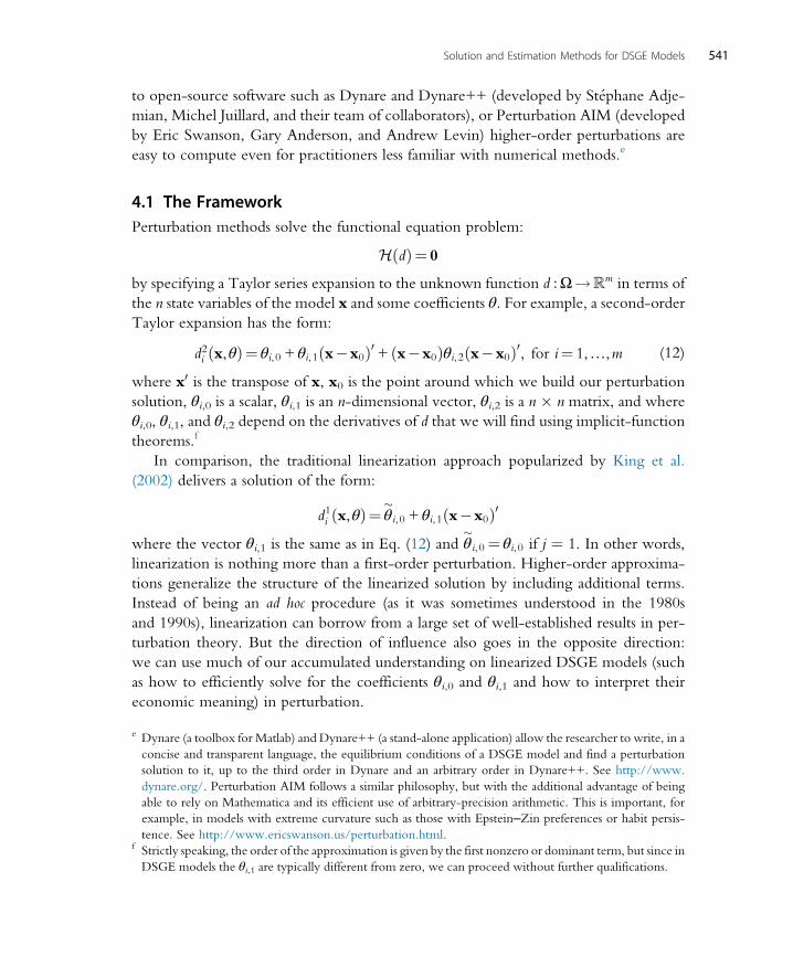
4.1 The FrameworkPerturbation methods solve the functional equation problem:

H dð Þ¼ 0

by specifying a Taylor series expansion to the unknown function d :Ω!m in terms of

the n state variables of the model x and some coefficients θ. For example, a second-order

Taylor expansion has the form:

d2i x,θð Þ¼ θi,0 + θi,1 x�x0ð Þ0 + x�x0ð Þθi,2 x�x0ð Þ0, for i¼ 1,…,m (12)

where x0 is the transpose of x, x0 is the point around which we build our perturbation

solution, θi,0 is a scalar, θi,1 is an n-dimensional vector, θi,2 is a n � n matrix, and where

θi,0, θi,1, and θi,2 depend on the derivatives of d that we will find using implicit-function

theorems.f

In comparison, the traditional linearization approach popularized by King et al.

(2002) delivers a solution of the form:

d1i x,θð Þ¼ θ�i,0 + θi,1 x�x0ð Þ0

where the vector θi,1 is the same as in Eq. (12) and θ�i,0¼ θi,0 if j ¼ 1. In other words,

linearization is nothing more than a first-order perturbation. Higher-order approxima-

tions generalize the structure of the linearized solution by including additional terms.

Instead of being an ad hoc procedure (as it was sometimes understood in the 1980s

and 1990s), linearization can borrow from a large set of well-established results in per-

turbation theory. But the direction of influence also goes in the opposite direction:

we can use much of our accumulated understanding on linearized DSGE models (such

as how to efficiently solve for the coefficients θi,0 and θi,1 and how to interpret their

economic meaning) in perturbation.

e Dynare (a toolbox for Matlab) and Dynare++ (a stand-alone application) allow the researcher to write, in a

concise and transparent language, the equilibrium conditions of a DSGE model and find a perturbation

solution to it, up to the third order in Dynare and an arbitrary order in Dynare++. See http://www.

dynare.org/. Perturbation AIM follows a similar philosophy, but with the additional advantage of being

able to rely on Mathematica and its efficient use of arbitrary-precision arithmetic. This is important, for

example, in models with extreme curvature such as those with Epstein–Zin preferences or habit persis-

tence. See http://www.ericswanson.us/perturbation.html.f Strictly speaking, the order of the approximation is given by the first nonzero or dominant term, but since in

DSGE models the θi,1 are typically different from zero, we can proceed without further qualifications.


http://www.dynare.org/

http://www.dynare.org/

http://www.ericswanson.us/perturbation.html

Remark 4 (Linearization vs loglinearization) Linearization and, more generally, per-

turbation, can be performed in the level of the state variables or after applying some

change of variables to any (or all) the variables of the model. Loglinearization, for

example, approximates the solution of the model in terms of the log-deviations of

the variables with respect to their steady state. That is, for a variable x 2 x,

we define:

x¼ logx

�x

where �x is its steady-state value, and then we find a second-order approximation:

d2i x,θð Þ¼ θi,0 + θi,1 x� x0ð Þ0 + x� x0ð Þθi,2 x� x0ð Þ0, for i¼ 1,…,m:

If x0 is the deterministic steady state (this is more often than not the case), x0¼ 0, since for

all variables x 2 x

x0¼ logx

�x¼ 0:

This result provides a compact representation:

d2i x,θð Þ¼ θi,0 + θi,1x0 + xθi,2x0, for i¼ 1,…,m:

Loglinear solutions are easy to read (the loglinear deviation is an approximation of the

percentage deviation with respect to the steady state) and, in some circumstances, they

can improve the accuracy of the solution. We will revisit the change of variables later in

the chapter.

Before getting into technical details of how to implement perturbation methods, we will

briefly distinguish between regular and singular perturbations. A regular perturbation is a

situation where a small change in the problem induces a small change in the solution. An

example is a standard New Keynesian model (Woodford, 2003). A small change in the

standard deviation of the monetary policy shock will lead to a small change in the

properties of the equilibrium dynamics (ie, the standard deviation and autocorrelation

of variables such as output or inflation). A singular perturbation is a situation where a

small change in the problem induces a large change in the solution. An example can

be an excess demand function. A small change in the excess demand function may lead

to an arbitrarily large change in the price that clears the market.

Many problems involving DSGE models will result in regular perturbations. Thus,

we will concentrate on them. But this is not necessarily the case. For instance, introduc-

ing a new asset in an incomplete market model can lead to large changes in the solution.

As researchers pay more attention to models with financial frictions and/or market

incompleteness, this class of problems may become common. Researchers will need

to learn more about how to apply singular perturbations. See, for pioneering work,


Judd and Guu (1993), and a presentation of bifurcation methods for singular problems in

Judd (1998).

4.2 The General CaseWe are now ready to deal with the details of how to implement a perturbation. We pre-

sent first the general case of how to find a perturbation solution of a DSGE model by (1)

using the equilibrium conditions of the model and (2) by finding a higher-order Taylor

series approximation. Once we have mastered this task, it would be straightforward to

extend the results to other problems, such as the solution of a value function, and to

conceive other possible perturbation schemes. This section follows much of the structure

and notation of section 3 in Schmitt-Groh�e and Uribe (2004).

We start by writing the equilibrium conditions of the model as

tHðy,y0,x,x0Þ ¼ 0, (13)

where y is an ny� 1 vector of controls, x is an nx� 1 vector of states, and n¼ nx+ ny. The

operator H :ny �ny �nx �nx !n stacks all the equilibrium conditions, some of

which will have expectational terms, some of which will not. Without loss of generality,

and with a slight change of notation with respect to Section 3, we place the conditional

expectation operator outside H: for those equilibrium conditions without expectations,

the conditional expectation operator will not have any impact. Moving t outsideHwill

make some of the derivations below easier to follow. Also, to save on space, when there is

no ambiguity, we will employ the recursive notation where x represents a variable at

period t and x0 a variable at period t + 1.

It will also be convenient to separate the endogenous state variables (capital, asset

positions, etc.) from the exogenous state variables (productivity shocks, preference

shocks, etc.). In that way, it will be easier to see the variables on which the perturbation

parameter that we will introduce below will have a direct effect. Thus, we partition the

state vector x (and taking transposes) as

x¼ ½x01; x02�0:where x1 is an nx�nEð Þ�1 vector of endogenous state variables and x2 is an nE �1 vector

of exogenous state variables. Let ~n¼ nx�nE.

4.2.1 Steady StateIf we suppress the stochastic component of the model (more details below), we can define

the deterministic steady-state of the model as vectors ð�x,�yÞ such that:

Hð�y,�y,�x,�xÞ¼ 0: (14)

The solution ð�x,�yÞ of this problem can often be found analytically. When this cannot be

done, it is possible to resort to a standard nonlinear equation solver.


The previous paragraph glossed over the possibility that the model we are dealing

with either does not have a steady state or that it has several of them (in fact, we can even

have a continuum of steady states). Given our level of abstraction with the definition of

Eq. (13), we cannot rule out any of these possibilities. Galor (2007) discusses in detail the

existence and stability (local and global) of steady states in discrete time dynamic models.

A case of interest is when the model, instead of having a steady state, has a balanced

growth path (BGP): that is, when the variables of the model (with possibly some excep-

tions such as labor) grow at the same rate (either deterministic or stochastic). Given that

perturbation is an inherently local solution method, we cannot deal directly with solving

such a model. However, on many occasions, we can rescale the variables xt in the model

by the trend μt:

xt ¼ xt

μt

to render them stationary (the trend itself may be a complicated function of some tech-

nological processes in the economy, as when we have both neutral and investment-

specific technological change; see Fernandez-Villaverde and Rubio-Ramırez, 2007).

Then, we can undertake the perturbation in the rescaled variable xt and undo the rescal-

ing when using the approximated solution for analysis and simulation.g

Remark 5 (Simplifying the solution of ð�x,�yÞ) Finding the solution ð�x,�yÞ can often be

made much easier by using two “tricks.” One is to substitute some of the variables away

from the operator H �ð Þ and reduce the system from being one of n equations in n

unknowns into a system of n0 < n equations in n0 unknowns. For example, if we have

a law of motion for capital involving capital next period, capital next period, and

investment:

kt+1¼ 1�δð Þkt + it

we can substitute out investment throughout the whole system just by writing:

it ¼ kt+1� 1�δð Þkt:Since the complexity of solving a nonlinear system of equations grows exponentially in

the dimension of the problem (see Sikorski, 1985, for classic results on computational

complexity), even a few substitutions can produce considerable improvements.

A second possibility is to select parameter values to pin down one or more variables of

the model and then to solve all the other variables as a function of the fixed variables. To

illustrate this point, let us consider a simple stochastic neoclassical growth model with a

representative household with utility function:

g This rescaling is also useful with projection methods since they need a bounded domain of the state

variables.


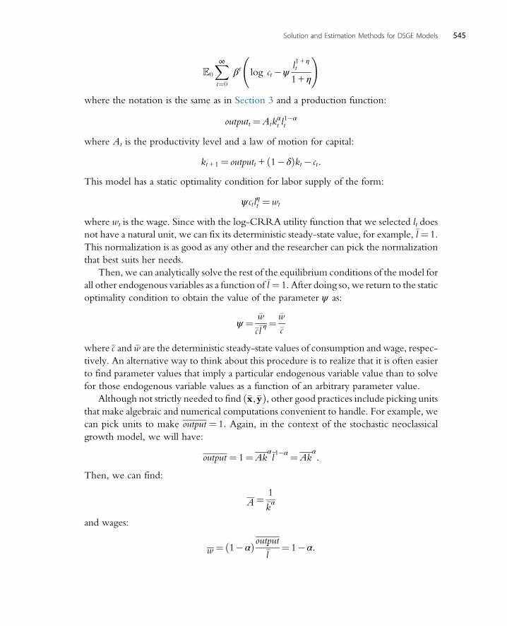
0

X∞t¼0

βt log ct�ψl1+ ηt

1+ η

!

where the notation is the same as in Section 3 and a production function:

outputt ¼Atkαt l1�αt

where At is the productivity level and a law of motion for capital:

kt+1 ¼ outputt + ð1�δÞkt� ct:

This model has a static optimality condition for labor supply of the form:

ψ ctlηt ¼wt

where wt is the wage. Since with the log-CRRA utility function that we selected lt does

not have a natural unit, we can fix its deterministic steady-state value, for example, �l ¼ 1.

This normalization is as good as any other and the researcher can pick the normalization

that best suits her needs.

Then, we can analytically solve the rest of the equilibrium conditions of the model for

all other endogenous variables as a function of �l ¼ 1. After doing so, we return to the static

optimality condition to obtain the value of the parameter ψ as:

ψ ¼ �w

�c�lη¼

�w

�c

where�c and �w are the deterministic steady-state values of consumption and wage, respec-

tively. An alternative way to think about this procedure is to realize that it is often easier

to find parameter values that imply a particular endogenous variable value than to solve

for those endogenous variable values as a function of an arbitrary parameter value.

Although not strictly needed to find ð�x,�yÞ, other good practices include picking unitsthat make algebraic and numerical computations convenient to handle. For example, we

can pick units to make output ¼ 1: Again, in the context of the stochastic neoclassical

growth model, we will have:

output ¼ 1¼Akα�l

1�α¼Akα:

Then, we can find:

A¼ 1

�kα

and wages:

w ¼ 1�αð Þoutput�l¼ 1�α:


Going back to the intertemporal Euler equation:

1

�c¼ 1

�cβ 1+�r �δð Þ

where r is the rental rate of capital and δ is depreciation, we find:

�r ¼ 1

β�1+ δ:

Since:

�r ¼ αoutput

�k¼ α

�kwe get:

�k¼ α1

β�1+ δ

and:

�c ¼ output�δ�k¼ 1�δα

1

β�1+ δ

,

from which:

ψ ¼w

�c¼ 1�α

1�δα

1

β�1+ δ

In this example, two judicious choices of units (�l ¼ output ¼ 1) render the solution of the

deterministic steady state a straightforward exercise. While the deterministic steady state

of more complicated models would be harder to solve, experience suggests that following

the advice in this remark dramatically simplifies the task in many situations.

The deterministic steady state ð�x,�yÞ is different from a fixed point ðx, yÞ of (13):tHðy, y, x, xÞ¼ 0,

because in the former case we eliminate the conditional expectation operator while in the

latter we do not. The vector ðx, yÞ is sometimes known as the stochastic steady state

(although, since we find the idea of mixing the words “stochastic” and “steady state”

in the same term confusing, we will avoid that terminology).

4.2.2 Exogenous Stochastic ProcessFor the exogenous stochastic variables, we specify a stochastic process of the form:

x02¼Cðx2Þ+ σηEE0 (15)


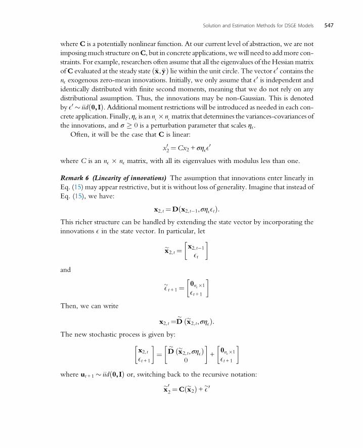
whereC is a potentially nonlinear function. At our current level of abstraction, we are not

imposingmuch structure onC, but in concrete applications,wewill need to addmore con-

straints. For example, researchers often assume that all the eigenvalues of theHessianmatrix

ofC evaluated at the steady state ð�x,�yÞ lie within the unit circle. The vector E0 contains thenE exogenous zero-mean innovations. Initially, we only assume that E0 is independent andidentically distributed with finite second moments, meaning that we do not rely on any

distributional assumption. Thus, the innovations may be non-Gaussian. This is denoted

by E0 � iid 0,Ið Þ. Additional moment restrictions will be introduced as needed in each con-

crete application. Finally, ηE is an nE �nE matrix that determines the variances-covariances of

the innovations, and σ � 0 is a perturbation parameter that scales ηE.Often, it will be the case that C is linear:

x02¼Cx2 + σηEE0

where C is an nE � nE matrix, with all its eigenvalues with modulus less than one.

Remark 6 (Linearity of innovations) The assumption that innovations enter linearly in

Eq. (15) may appear restrictive, but it is without loss of generality. Imagine that instead of

Eq. (15), we have:

x2, t ¼Dðx2, t�1,σηEEtÞ:This richer structure can be handled by extending the state vector by incorporating the

innovations E in the state vector. In particular, let

x�2, t ¼ x2, t�1

Et

�

and

E�t+1 ¼ 0nE�1

Et+1

�

Then, we can write

x2, t ¼D� ðx�2, t,σηEÞ:

The new stochastic process is given by:

x2, tEt+1

� ¼ D

� ðx�2, t,σηEÞ0

� +

0nE�1

Et+1

�

where ut+1� iid 0,Ið Þ or, switching back to the recursive notation:

x�02¼Cðx�2Þ+ E�0


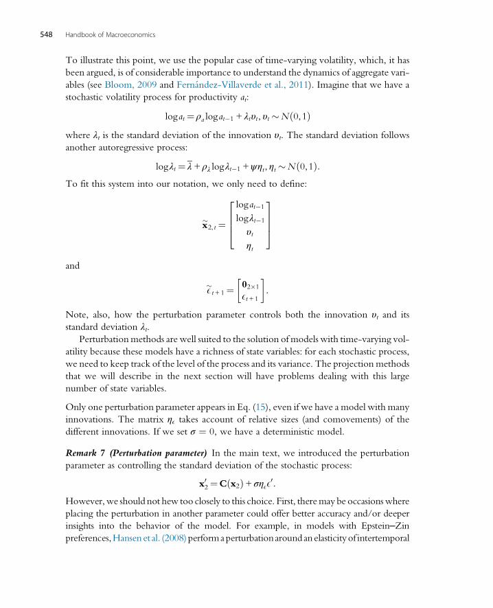
To illustrate this point, we use the popular case of time-varying volatility, which, it has

been argued, is of considerable importance to understand the dynamics of aggregate vari-

ables (see Bloom, 2009 and Fernandez-Villaverde et al., 2011). Imagine that we have a

stochastic volatility process for productivity at:

logat ¼ ρa logat�1 + λtυt, υt �N 0,1ð Þwhere λt is the standard deviation of the innovation υt. The standard deviation follows

another autoregressive process:

logλt ¼ λ + ρλ logλt�1 +ψηt, ηt �N 0,1ð Þ:To fit this system into our notation, we only need to define:

x�2, t ¼

logat�1

logλt�1

υtηt

2664

3775

and

E�t+1¼ 02�1

Et+1

� :

Note, also, how the perturbation parameter controls both the innovation υt and its

standard deviation λt.Perturbationmethods are well suited to the solution of models with time-varying vol-

atility because these models have a richness of state variables: for each stochastic process,

we need to keep track of the level of the process and its variance. The projection methods

that we will describe in the next section will have problems dealing with this large

number of state variables.

Only one perturbation parameter appears in Eq. (15), even if we have a model with many

innovations. The matrix ηE takes account of relative sizes (and comovements) of the

different innovations. If we set σ ¼ 0, we have a deterministic model.

Remark 7 (Perturbation parameter) In the main text, we introduced the perturbation

parameter as controlling the standard deviation of the stochastic process:

x02¼Cðx2Þ+ σηEE0:

However,we should not hew too closely to this choice. First, theremay be occasionswhere

placing the perturbation in another parameter could offer better accuracy and/or deeper

insights into the behavior of the model. For example, in models with Epstein–Zin

preferences,Hansenet al. (2008)performaperturbationaroundanelasticityof intertemporal


substitution equal to 1. Also, the choice of perturbation would be different in a continuous

time model, where it is usually more convenient to control the variance.

We depart from Samuelson (1970) and Jin and Judd (2002), who impose a bounded sup-

port for the innovations of the model. By doing so, these authors avoid problems with the

stability of the simulations coming from the perturbation solution that we will discuss

below. Instead, we will introduce pruning as an alternative strategy to fix these problems.

4.2.3 Solution of the ModelThe solution of the model will be given by a set of decision rules for the control variables

y¼ g x; σð Þ, (16)

and for the state variables

x0 ¼h x; σð Þ+ σηE0, (17)

where g maps nx �+ into Rny and h maps nx �+ into nx . Note our timing con-

vention: controls depend on current states, while states next period depend on states

today and the innovations tomorrow. By defining additional state variables that store

the information of states with leads and lags, this structure is sufficiently flexible to capture

rich dynamics. Also, we separate states x and the perturbation parameter σ by a semicolon

to emphasize the difference between both elements.

The nx � nE matrix η is:

η¼ ;ηE

�

where the first nx rows come from the states today determining the endogenous states

tomorrow and the last nE rows come from the exogenous states tomorrow depending

on the states today and the innovations tomorrow.

The goal of perturbation is to find a Taylor series expansion of the functions g and h

around an appropriate point. A natural candidate for this point is the deterministic steady

state, xt ¼ �x and σ ¼ 0. As we argued above, we know how to compute this steady state

and, consequently, how to evaluate the derivatives of the operator H �ð Þ that we will

require.

First, note by the definition of the deterministic steady state (14) we have that

�y¼ gð�x; 0Þ (18)

and

�x¼hð�x; 0Þ: (19)

Second, we plug-in the unknown solution on the operator H and define the new

operator F :nx +1!n:


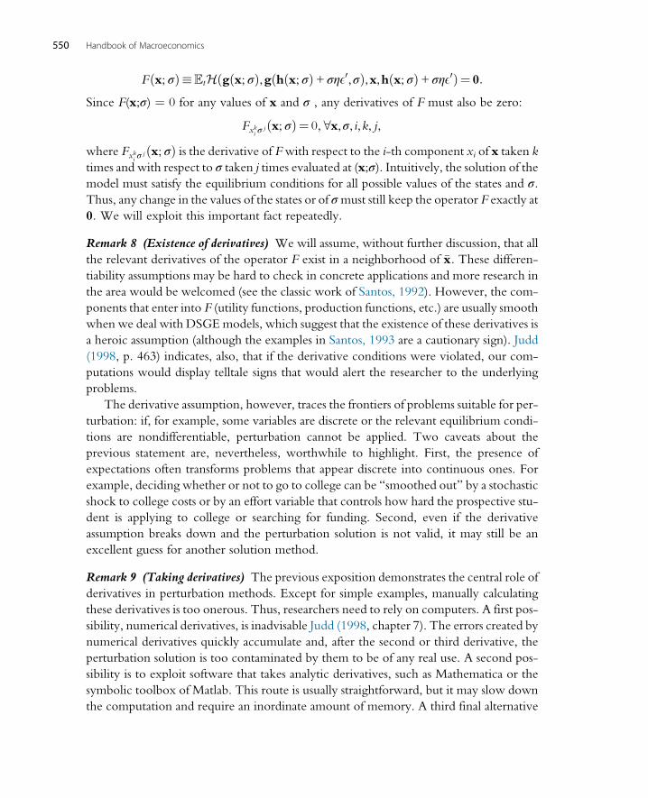
Fðx; σÞtHðgðx; σÞ,gðh x; σð Þ+ σηE0,σÞ,x,h x; σð Þ+ σηE0Þ ¼ 0:

Since F(x;σ) ¼ 0 for any values of x and σ , any derivatives of F must also be zero:

Fxki σjðx; σÞ¼ 0, 8x,σ, i,k, j,

where Fxki σjðx; σÞ is the derivative of Fwith respect to the i-th component xi of x taken k

times and with respect to σ taken j times evaluated at (x;σ). Intuitively, the solution of themodel must satisfy the equilibrium conditions for all possible values of the states and σ.Thus, any change in the values of the states or of σmust still keep the operator F exactly at

0. We will exploit this important fact repeatedly.

Remark 8 (Existence of derivatives) We will assume, without further discussion, that all

the relevant derivatives of the operator F exist in a neighborhood of �x. These differen-tiability assumptions may be hard to check in concrete applications and more research in

the area would be welcomed (see the classic work of Santos, 1992). However, the com-

ponents that enter into F (utility functions, production functions, etc.) are usually smooth

when we deal with DSGEmodels, which suggest that the existence of these derivatives is

a heroic assumption (although the examples in Santos, 1993 are a cautionary sign). Judd

(1998, p. 463) indicates, also, that if the derivative conditions were violated, our com-

putations would display telltale signs that would alert the researcher to the underlying

problems.

The derivative assumption, however, traces the frontiers of problems suitable for per-

turbation: if, for example, some variables are discrete or the relevant equilibrium condi-

tions are nondifferentiable, perturbation cannot be applied. Two caveats about the

previous statement are, nevertheless, worthwhile to highlight. First, the presence of

expectations often transforms problems that appear discrete into continuous ones. For

example, deciding whether or not to go to college can be “smoothed out” by a stochastic

shock to college costs or by an effort variable that controls how hard the prospective stu-

dent is applying to college or searching for funding. Second, even if the derivative

assumption breaks down and the perturbation solution is not valid, it may still be an

excellent guess for another solution method.

Remark 9 (Taking derivatives) The previous exposition demonstrates the central role of

derivatives in perturbation methods. Except for simple examples, manually calculating

these derivatives is too onerous. Thus, researchers need to rely on computers. A first pos-

sibility, numerical derivatives, is inadvisable Judd (1998, chapter 7). The errors created by

numerical derivatives quickly accumulate and, after the second or third derivative, the

perturbation solution is too contaminated by them to be of any real use. A second pos-

sibility is to exploit software that takes analytic derivatives, such as Mathematica or the

symbolic toolbox of Matlab. This route is usually straightforward, but it may slow down

the computation and require an inordinate amount of memory. A third final alternative


is to employ automatic differentiation, a technique that takes advantage of the application

of the chain rule to a series of elementary arithmetic operations and functions (for

how automatic differentiation can be applied to DSGE models, see Bastani and

Guerrieri, 2008).

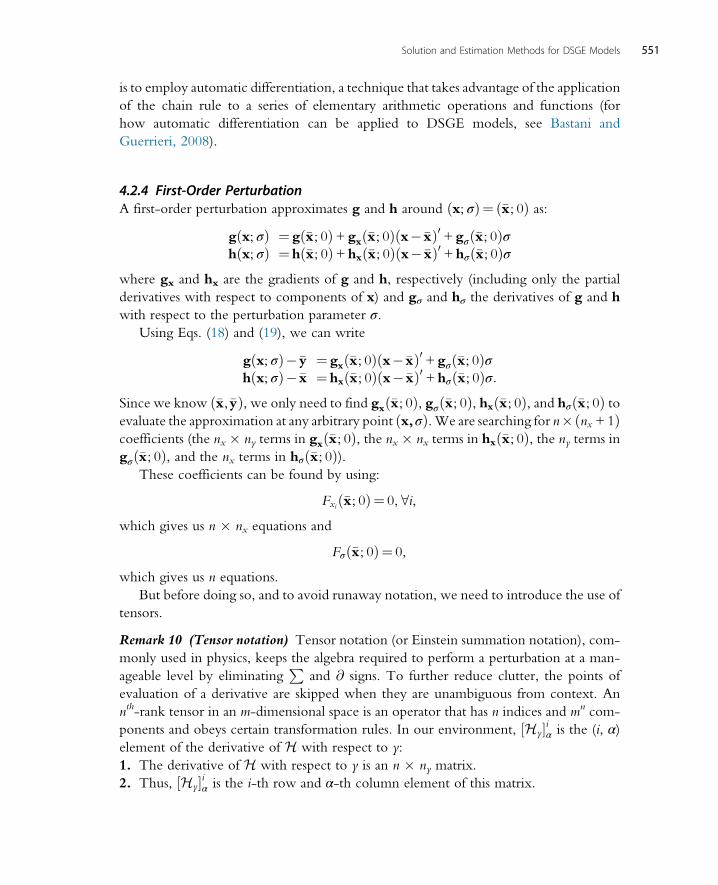
4.2.4 First-Order PerturbationA first-order perturbation approximates g and h around ðx; σÞ¼ ð�x; 0Þ as:

gðx; σÞ ¼ gð�x; 0Þ+ gxð�x; 0Þðx��xÞ0 + gσð�x; 0Þσhðx; σÞ ¼hð�x; 0Þ+hxð�x; 0Þðx��xÞ0 +hσð�x; 0Þσ

where gx and hx are the gradients of g and h, respectively (including only the partial

derivatives with respect to components of x) and gσ and hσ the derivatives of g and h

with respect to the perturbation parameter σ.Using Eqs. (18) and (19), we can write

gðx; σÞ��y ¼ gxð�x; 0Þðx��xÞ0 + gσð�x; 0Þσhðx; σÞ� �x ¼hxð�x; 0Þðx��xÞ0 +hσð�x; 0Þσ:

Since we know ð�x,�yÞ, we only need to find gxð�x; 0Þ, gσð�x; 0Þ, hxð�x; 0Þ, and hσð�x; 0Þ toevaluate the approximation at any arbitrary point x,σð Þ.We are searching for n� nx +1ð Þcoefficients (the nx � ny terms in gxð�x; 0Þ, the nx � nx terms in hxð�x; 0Þ, the ny terms in

gσð�x; 0Þ, and the nx terms in hσð�x; 0Þ).These coefficients can be found by using:

Fxið�x; 0Þ¼ 0, 8i,which gives us n � nx equations and

Fσð�x; 0Þ¼ 0,

which gives us n equations.

But before doing so, and to avoid runaway notation, we need to introduce the use of

tensors.

Remark 10 (Tensor notation) Tensor notation (or Einstein summation notation), com-

monly used in physics, keeps the algebra required to perform a perturbation at a man-

ageable level by eliminatingP

and @ signs. To further reduce clutter, the points of

evaluation of a derivative are skipped when they are unambiguous from context. An

nth-rank tensor in an m-dimensional space is an operator that has n indices and mn com-

ponents and obeys certain transformation rules. In our environment, ½Hy�iα is the (i, α)element of the derivative of H with respect to y:

1. The derivative of H with respect to y is an n � ny matrix.

2. Thus, ½Hy�iα is the i-th row and α-th column element of this matrix.


3. When a subindex appears as a superindex in the next term, we are omitting a sum

operator. For example,

½Hy�iα½gx�αβ½hx�βj ¼Xnyα¼1

Xnxβ¼1

@Hi

@yα@gα

@xβ@hβ

@xj:

4. The generalization to higher derivatives is direct. If we have ½Hy0y0 �iαγ:(a) Hy0y0 is a three-dimensional array with n rows, ny columns, and ny pages.

(b) Thus, ½Hy0y0 �iαγ denotes the i-th row, α-th column element, and γ-th page of this

matrix.

With the tensor notation, we can get into solving the system. First, gxð�x; 0Þ and hxð�x; 0Þare the solution to:

½Fxð�x; 0Þ�ij ¼ ½Hy0 �iα½gx�αβ½hx�βj + ½Hy�iα½gx�αj + ½Hx0 �iβ½hx�βj + ½Hx�ij ¼ 0;

i¼ 1,…,n; j,β¼ 1,…,nx; α¼ 1,…,ny:(20)

The derivatives of H evaluated at ðy,y0,x,x0Þ ¼ ð�y,�y,�x,�xÞ are known. Therefore,

we have a system of n � nx quadratic equations in the n � nx unknowns given by the

elements of gxð�x; 0Þ and hxð�x; 0Þ. After some algebra, the system (20) can be written as:

AP2�BP�C¼ 0

where the ~n� ~n matrix A, the ~n� ~n matrix B and the ~n� ~n matrix C involve terms from

½Hy0 �iα, ½Hy�iα, ½Hx0 �iβ, and ½Hx�ij and the ~n� ~nmatrix P the terms ½hx�βj related to the law of

motion of x1 (in our worked-out example of the next subsection, we will make this alge-

bra explicit). We can solve this system with a standard quadratic matrix equation solver.

Remark 11 (Quadratic equation solvers) The literature has proposed several procedures

to solve quadratic systems. Without being exhaustive, we can list Blanchard and Kahn

(1980), King and Watson (1998), Uhlig (1999), Klein (2000), and Sims (2002). These

different approaches vary in the details of how the solution to the system is found and

how general they are (regarding the regularity conditions they require). But, conditional

on applicability, all methods find the same policy functions since the linear space approx-

imating a nonlinear space is unique.

For concision, we will only present one of the simplest of these procedures, as

discussed by Uhlig (1999, pp. 43–45). Given

AP2�BP�C¼ 0,

define the 2~n�2~n matrix:

D¼ A 0~n0~n I~n

�


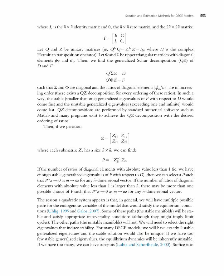
where I~n is the ~n� ~n identity matrix and 0~n the ~n� ~n zero matrix, and the 2~n�2~nmatrix:

F ¼ B C

In 0n

�

Let Q and Z be unitary matrices (ie, QHQ¼ZHZ¼ I2~n where H is the complex

Hermitian transposition operator). LetΦ andΣ be upper triangularmatriceswith diagonal

elements ϕii and σii. Then, we find the generalized Schur decomposition (QZ) of

D and F:

Q0ΣZ¼D

Q0ΦZ¼F

such that Σ andΦ are diagonal and the ratios of diagonal elements ϕii=σiij j are in increas-ing order (there exists a QZ decomposition for every ordering of these ratios). In such a

way, the stable (smaller than one) generalized eigenvalues of F with respect to D would

come first and the unstable generalized eigenvalues (exceeding one and infinite) would

come last. QZ decompositions are performed by standard numerical software such as

Matlab and many programs exist to achieve the QZ decomposition with the desired

ordering of ratios.

Then, if we partition:

Z¼ Z11 Z12

Z21 Z22

�

where each submatrix Zii has a size ~n� ~n, we can find:

P¼�Z�121 Z22:

If the number of ratios of diagonal elements with absolute value less than 1 (ie, we have

enough stable generalized eigenvalues of Fwith respect toD), then we can select a P such

that Pmx! 0 as m!∞ for any ~n-dimensional vector. If the number of ratios of diagonal

elements with absolute value less than 1 is larger than ~n, there may be more than one

possible choice of P such that Pmx! 0 as m!∞ for any ~n-dimensional vector.

The reason a quadratic system appears is that, in general, we will have multiple possible

paths for the endogenous variables of the model that would satisfy the equilibrium condi-

tions (Uhlig, 1999 andGalor, 2007). Some of these paths (the stablemanifolds) will be sta-

ble and satisfy appropriate transversality conditions (although they might imply limit

cycles). The other paths (the unstable manifolds) will not. We will need to select the right

eigenvalues that induce stability. For many DSGE models, we will have exactly ~n stablegeneralized eigenvalues and the stable solution would also be unique. If we have too

few stable generalized eigenvalues, the equilibrium dynamics will be inherently unstable.

If we have too many, we can have sunspots (Lubik and Schorfheide, 2003). Suffice it to


note here that all these issueswould depend only on the first-order approximation and that

going to higher-order approximations would not change the issues at hand. If we have

uniqueness of equilibrium in the first-order approximation, we will also have uniqueness

in the second-order approximation. And if we have multiplicity of equilibria in the first-

order approximation, we will also have multiplicity in the second-order approximation.

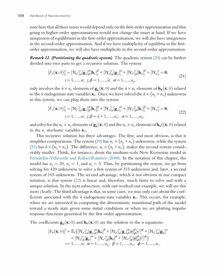
Remark 12 (Partitioning the quadratic system) The quadratic system (20) can be further

divided into two parts to get a recursive solution. The system:


i¼ 1,…,n; j,β¼ 1,…,~n; α¼ 1,…,ny:(21)

only involves the ~n�ny elements of gxð�x; 0Þ and the ~n�nx elements of hxð�x; 0Þ relatedto the ~n endogenous state variables x1. Once we have solved the ~n� ny + nx

� �unknowns

in this system, we can plug them into the system:


i¼ 1,…,n; j,β¼ ~n+1,…,nx; α¼ 1,…,ny:(22)

and solve for the nE� ny elements of gxð�x; 0Þ and the nE� nx elements of hxð �x; 0ð Þ relatedto the nE stochastic variables x2.

This recursive solution has three advantages. The first, and most obvious, is that it

simplifies computations. The system (20) has nx� ny + nx� �

unknowns, while the system

(21) has ~n� ny + nx� �

. The difference, nE� ny + nx� �

, makes the second system consid-

erably smaller. Think, for instance, about the medium-scale New Keynesian model in

Fernandez-Villaverde and Rubio-Ramırez (2008). In the notation of this chapter, the

model has nx ¼ 20, ny ¼ 1, and nE ¼ 5. Thus, by partitioning the system, we go from

solving for 420 unknowns to solve a first system of 315 unknowns and, later, a second

system of 105 unknowns. The second advantage, which is not obvious in our compact

notation, is that system (22) is linear and, therefore, much faster to solve and with a

unique solution. In the next subsection, with our worked-out example, we will see this

more clearly. The third advantage is that, in some cases, wemay only care about the coef-

ficients associated with the ~n endogenous state variables x1. This occurs, for example,

when we are interested in computing the deterministic transitional path of the model

toward a steady state given some initial conditions or when we are plotting impulse

response functions generated by the first-order approximation.

The coefficients gσð�x; 0Þ and hσð�x; 0Þ are the solution to the n equations:

½Fσð�x; 0Þ�i¼tf½Hy0 �iα½gx�αβ½hσ�β + ½Hy0 �iα½gx�αβ½η�βϕ½E0�ϕ + ½Hy0 �iα½gσ�α+ ½Hy�iα½gσ�α + ½Hx0 �iβ½hσ�β + ½Hx0 �iβ½η�βϕ½E0�ϕg

i¼ 1,…,n; α¼ 1,…,ny; β¼ 1,…,nx; ϕ¼ 1,…,nE:


Then:

½Fσð�x; 0Þ�i¼ ½Hy0 �iα½gx�αβ½hσ�β + ½Hy0 �iα½gσ�α + ½Hy�iα½gσ�α + ½ fx0 �iβ½hσ�β ¼ 0;

i¼ 1,…,n; α¼ 1,…,ny; β¼ 1,…,nx; ϕ¼ 1,…,nE:

Inspection of the previous equations shows that they are linear and homogeneous equa-

tions in gσ and hσ. Thus, if a unique solution exists, it satisfies:

gσ ¼ 0

hσ ¼ 0

In other words, the coefficients associated with the perturbation parameter are zero and

the first-order approximation is

gðx; σÞ��y¼ gxð�x; 0Þðx� �xÞ0hðx; σÞ� �x¼hxð�x; 0Þðx� �xÞ0:

These equations embody certainty equivalence as defined by Simon (1956) and Theil

(1957). Under certainty equivalence, the solution of the model, up to first-order, is iden-

tical to the solution of the same model under perfect foresight (or under the assumption

that σ ¼ 0). Certainty equivalence does not preclude the realization of the shock from

appearing in the decision rule. What certainty equivalence precludes is that the standard

deviation of it appears as an argument by itself, regardless of the realization of the shock.

The intuition for the presence of certainty equivalence is simple. Risk-aversion

depends on the second derivative of the utility function (concave utility). However,

Leland (1968) and Sandmo (1970) showed that precautionary behavior depends on

the third derivative of the utility function. But a first-order perturbation involves

the equilibrium conditions of the model (which includes first derivatives of the utility

function, for example, in the Euler equation that equates marginal utilities over time)

and first derivatives of these equilibrium conditions (and, therefore, second derivatives

of the utility function), but not higher-order derivatives.

Certainty equivalence has several drawbacks. First, it makes it difficult to talk about

the welfare effects of uncertainty. Although the dynamics of the model are still partially

driven by the variance of the innovations (the realizations of the innovations depend on

it), the agents in the model do not take any precautionary behavior to protect themselves

from that variance, biasing any welfare computation. Second, related to the first point,

the approximated solution generated under certainty equivalence cannot generate any

risk premia for assets, a strongly counterfactual prediction.h Third, certainty equivalence

prevents researchers from analyzing the consequences of changes in volatility.

h In general equilibrium, there is an intimate link between welfare computations and asset pricing. An exer-

cise on the former is always implicitly an exercise on the latter (see Alvarez and Jermann, 2004).


Remark 13 (Perturbation and LQ approximations) Kydland and Prescott (1982)—and

many papers after them—took a different route to solving DSGE models. Imagine that

we have an optimal control problem that depends on nx states xt and nu control variables

ut. To save on notation, let us also define the column vector wt ¼ xt , ut½ �0 of dimension

nw ¼ nx + nu. Then, we can write the optimal control problem as:

max 0

X∞t¼0

βtr wtð Þs:t: xt+1¼A wt,εtð Þ

where r is a return function, εt a vector of nε innovations with zero mean and finite var-

iance, and A summarizes all the constraints and laws of motion of the economy. By

appropriately enlarging the state space, this notation can accommodate the innovations

having an impact on the period return function and some variables being both controls

and states.

In the case where the return function r is quadratic, ie,

r wtð Þ¼B0 +B1wt +w0tQwt

(where B0 is a constant, B1 a row vector 1 � nw, and B2 is an nw � nw matrix) and the

function A is linear:

xt+1¼B3wt +B4εt

(where B3 is an nx � nw matrix and B4 is an nx � nε matrix), we are facing a stochastic

discounted linear-quadratic regulator (LQR) problem. There is a large and well-developed

research area on LQR problems. This literature is summarized by Anderson et al. (1996)

and Hansen and Sargent (2013). In particular, we know that the optimal decision rule in

this environment is a linear function of the states and the innovations:

ut ¼Fwwt +Fεεt

where Fw can be found by solving a Ricatti equation Anderson et al. (1996, pp. 182–183)

and Fε by solving a Sylvester equation Anderson et al. (1996, pp. 202–205). Interestingly,

Fw is independent of the variance of εt. That is, if εt has a zero variance, then the optimal

decision rule is simply:

ut ¼Fwwt:

This neat separation between the computation of Fw and of Fε allows the researcher to

deal with large problems with ease. However, it also implies certainty equivalence.

Kydland and Prescott (1982) setup the social planner’s problem of their economy,

which fits into an optimal regulator problem, and they were able to write a function

A that was linear in wt, but they did not have a quadratic return function. Instead, they

took a quadratic approximation to the objective function of the social planner. Most of


the literature that followed them used a Taylor series approximation of the objective

function around the deterministic steady state, sometimes called the approximated

LQR problem (Kydland and Prescott also employed a slightly different point of approx-

imation that attempted to control for uncertainty; this did not make much quantitative

difference). Furthermore, Kydland and Prescott worked with the value function repre-

sentation of the problem. See Dıaz-Gim�enez (1999) for an explanation of how to deal

with the LQ approximation to the value function.

The result of solving the approximated LQR when the function A is linear is equiv-

alent to the result of a first-order perturbation of the equilibrium conditions of the

model. The intuition is simple. Derivatives are unique, and since both approaches

search for a linear approximation to the solution of the model, they have to yield

identical results.

However, approximated LQR have lost their popularity for three reasons. First, it

is often hard to write the function A in a linear form. Second, it is challenging to set

up a social planner’s problem when the economy is not Pareto efficient. And even

when it is possible to have a modified social planner’s problem that incorporates addi-

tional constraints that incorporate non-optimalities (see, for instance, Benigno and

Woodford, 2004), the same task is usually easier to accomplish by perturbing the equi-

librium conditions of the model. Third, and perhaps most important, perturbations

can easily go to higher-order terms and incorporate nonlinearities that break certainty

equivalence.

4.2.5 Second-Order PerturbationOnce we have finished the first-order perturbation, we can iterate on the steps before to

generate higher-order solutions. More concretely, the second-order approximations to g

around ðx; σÞ¼ ð�x; 0Þ are:½gðx; σÞ�i ¼ ½gð�x; 0Þ�i + ½gxð�x; 0Þ�ia½ðx�xÞ�a + ½gσð�x; 0Þ�i½σ�

+1

2½gxxð�x; 0Þ�iab½ðx� �xÞ�a½ðx��xÞ�b

+1

2½gxσð�x; 0Þ�ia½ðx� �xÞ�a½σ�

+1

2½gσxð�x; 0Þ�ia½ðx� �xÞ�a½σ�

+1

2½gσσð�x; 0Þ�i½σ�½σ�

where i¼ 1,…,ny, a,b¼ 1,…,nx, and j¼ 1,…,nx.

Similarly, the second-order approximations to h around ðx; σÞ¼ ð�x; 0Þ are:


½hðx; σÞ�j ¼ ½hð�x; 0Þ�j + ½hxð�x; 0Þ�ja½ðx�xÞ�a + ½hσð�x; 0Þ�j½σ�

+1

2½hxxð�x; 0Þ�jab½ðx��xÞ�a½ðx� �xÞ�b

+1

2½hxσð�x; 0Þ�ja½ðx� �xÞ�a½σ�

+1

2½hσxð�x; 0Þ�ja½ðx� �xÞ�a½σ�

+1

2½hσσð�x; 0Þ�j½σ�½σ�,

where i¼ 1,…,ny, a,b¼ 1,…,nx, and j¼ 1,…,nx.

The unknown coefficients in these approximations are ½gxx�iab, ½gxσ�ia, ½gσx�ia, [gσσ]i,½hxx�jab, ½hxσ�ja, ½hσx�ja, [hσσ]j. As before, we solve for these coefficients by taking the secondderivatives of F(x; σ) with respect to x and σ, making them equal to zero, and evaluating

them at ð�x; 0Þ.How do we solve the system? First, we exploit Fxxð�x; 0Þ to solve for gxxð�x; 0Þ and

hxxð�x; 0Þ:

½Fxxð�x; 0Þ�ijk ¼

½Hy0y0 �iαγ½gx�γδ½hx�δk + ½Hy0y�iαγ½gx�γk + ½Hy0x0 �iαδ½hx�δk + ½Hy0x�iαk� �

½gx�αβ½hx�βj+½Hy0 �iα½gxx�αβδ½hx�δk½hx�βj + ½Hy0 �iα½gx�αβ½hxx�βjk+ ½Hyy0 �iαγ½gx�γδ½hx�δk + ½Hyy�iαγ½gx�γk + ½Hyx0 �iαδ½hx�δk + ½Hyx�iαk� �

½gx�αj + ½Hy�iα½gxx�αjk+ ½Hx0y0 �iβγ½gx�γδ½hx�δk + ½Hx0y�iβγ½gx�γk + ½Hx0x0 �iβδ½hx�δk + ½Hx0x�iβk� �

½hx�βj + ½Hx0 �iβ½hxx�βjk+½Hxy0 �ijγ½gx�γδ½hx�δk + ½Hxy�ijγ½gx�γk + ½Hxx0 �ijδ½hx�δk + ½Hxx�ijk¼ 0;

i¼ 1,…n, j,k,β,δ¼ 1,…nx; α,γ¼ 1,…ny:

But we know the derivatives ofH.We also know the first derivatives of g and h evaluated

at ð�x, 0Þ. Hence, the above expression is a system of n � nx � nx linear equations in the

n� nx� nx unknown elements of gxx and hxx. This point is crucial: linear solvers are fast

and efficient. In the first-order approximation we had to solve a quadratic system to select

between stable and unstable solutions. But once we are already in the stable manifold,

there are no further additional solutions that we need to rule out. These quadratic

terms involve the endogenous state vector x1. Those terms capture nonlinear behavior

and induce nonsymmetries. We will discuss those in more detail in our worked-out

example below.


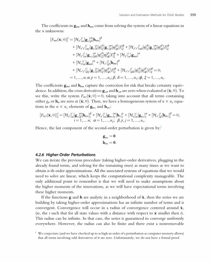
The coefficients in gσσ and hσσ come from solving the system of n linear equations in

the n unknowns:

½Fσσð�x; 0Þ�i¼ ½Hy0 �iα½gx�αβ½hσσ�β

+ ½Hy0y0 �iαγ½gx�γδ½η�δξ½gx�αβ½η�βϕ½I �ϕξ + ½Hy0x0 �iαδ½η�δξ½gx�αβ½η�βϕ½I �ϕξ+ ½Hy0 �iα½gxx�αβδ½η�δξ½η�βϕ½I �ϕξ + ½Hy0 �iα½gσσ�α

+ ½Hy�iα½gσσ�α + ½Hx0 �iβ½hσσ�β

+ ½Hx0y0 �iβγ½gx�γδ½η�δξ½η�βϕ½I �ϕξ + ½Hx0x0 �iβδ½η�δξ½η�βϕ½I �ϕξ ¼ 0;

¼ 1,…,n; α,γ¼ 1,…,ny; β, δ¼ 1,…,nx;ϕ, ξ¼ 1,…,nE:

The coefficients gσσ and hσσ capture the correction for risk that breaks certainty equiv-

alence. In addition, the cross derivatives gxσ and hxσ are zero when evaluated at ð�x; 0Þ. Tosee this, write the system Fσxð�x; 0Þ¼ 0, taking into account that all terms containing

either gσ or hσ are zero at ð�x; 0Þ. Then, we have a homogeneous system of n � nx equa-

tions in the n � nx elements of gσx and hσx:

½Fσxð�x; 0Þ�ij ¼ ½Hy0 �iα½gx�αβ½hσx�βj + ½Hy0 �iα½gσx�αγ ½hx�γj + ½Hy�iα½gσx�αj + ½Hx0 �iβ½hσx�βj ¼ 0;

i¼ 1,…n; α¼ 1,…,ny; β,γ, j¼ 1,…,nx:

Hence, the last component of the second-order perturbation is given by:i

gσx¼ 0

hσx¼ 0:

4.2.6 Higher-Order PerturbationsWe can iterate the previous procedure (taking higher-order derivatives, plugging in the

already found terms, and solving for the remaining ones) as many times as we want to

obtain n-th order approximations. All the associated systems of equations that we would

need to solve are linear, which keeps the computational complexity manageable. The

only additional point to remember is that we will need to make assumptions about

the higher moments of the innovations, as we will have expectational terms involving

these higher moments.

If the functions g and h are analytic in a neighborhood of �x, then the series we are

building by taking higher-order approximations has an infinite number of terms and is

convergent. Convergence will occur in a radius of convergence centered around �x,(ie, the r such that for all state values with a distance with respect to �x smaller then r).

This radius can be infinite. In that case, the series is guaranteed to converge uniformly

everywhere. However, the radius can also be finite and there exist a nonremovable

i We conjecture (and we have checked up to as high an order of a perturbation as computer memory allows)

that all terms involving odd derivatives of σ are zero. Unfortunately, we do not have a formal proof.


singularity on its boundary. Disappointingly, for most DSGE models, the radius of

convergence is unknown (for more details and examples, see Swanson et al., 2006

and Aldrich and Kung, 2011). More research on this topic is sorely needed. Also, even

when the series is convergent, there are two potential problems. First, at a j-th order

approximation, we may lose the “right” shape of g and h. For example, Aruoba et al.

(2006) document how the decision rules for consumption and capital of the stochastic

neoclassical growth model approximated with a fifth-order perturbation are no longer

globally concave, as implied by economic theory. Instead, the approximated functions

present oscillating patterns. Second, the convergence to the exact solution may not be

monotone: it is easy to build examples where the errors a bit away from �x are worse for

a j + 1-th order approximation than for a j-th order approximation. Neither of these

two problems is fatal, but the researcher needs to be aware of them and undertake the

necessary tests to minimize their impact (for instance, checking the solution for different

approximation orders).

Later, we will discuss how to gauge the accuracy of a solution and how to decide

whether a higher-order approximation is required. For example, to deal with models

with time-varying volatility, we would need at least a third-order approximation.

Levintal (2015a) has argued that to approximate well models with disaster risk, we need

a fifth-order approximation. The drawback of higher-order approximations is that we

will run into problems of computational cost and memory use.

4.3 A Worked-Out ExampleThe previous derivations were somewhat abstract and the notation, even using tensors,

burdensome. Consequently, it is useful to show how perturbation works in a concrete

example. For that, we come back to our example of the neoclassical growthmodel defined

by Eqs. (2)–(4), except that, to make the algebra easier, we assume u cð Þ¼ log c and δ¼ 1.

The equilibrium conditions of the model are then:

1

ct¼ βt

αezt+1kα�1t+1

ct+1

ct + kt+1¼ ezt kαt

zt ¼ ρzt�1 + ηεt

While this parameterization is unrealistic for periods of time such as a quarter or a year

typically employed in business cycle analysis, it has the enormous advantage of implying

that the model has a closed-form solution. With δ ¼ 1, the income and the substitution

effect from a productivity shock cancel each other, and consumption and investment are

constant fractions of income:

ct ¼ 1�αβð Þeztkαtkt+1 ¼ αβeztkαt


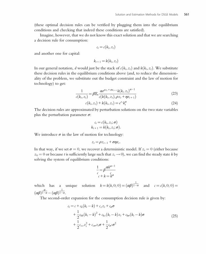
(these optimal decision rules can be verified by plugging them into the equilibrium

conditions and checking that indeed these conditions are satisfied).

Imagine, however, that we do not know this exact solution and that we are searching

a decision rule for consumption:

ct ¼ c kt,ztð Þand another one for capital:

kt+1¼ k kt,ztð ÞIn our general notation, d would just be the stack of c kt,ztð Þ and k kt,ztð Þ. We substitute

these decision rules in the equilibrium conditions above (and, to reduce the dimension-

ality of the problem, we substitute out the budget constraint and the law of motion for

technology) to get:

1

c kt,ztð Þ¼ βt

αeρzt + σεt+1k kt ,ztð Þα�1

c k kt,ztð Þ,ρzt + ηεt+1ð Þ (23)

c kt,ztð Þ+ k kt,ztð Þ¼ ezt kαt (24)

The decision rules are approximated by perturbation solutions on the two state variables

plus the perturbation parameter σ:

ct ¼ c kt,zt; σð Þkt+1¼ k kt,zt; σð Þ:

We introduce σ in the law of motion for technology:

zt ¼ ρzt�1 + σηεt:

In that way, if we set σ ¼ 0, we recover a deterministic model. If zt ¼ 0 (either because

z0¼ 0 or because t is sufficiently large such that zt ! 0), we can find the steady state k by

solving the system of equilibrium conditions:

1

c¼ β

αkα�1

cc + k¼ kα

which has a unique solution k¼ k k,0; 0ð Þ¼ αβð Þ 11�α and c¼ c k,0; 0ð Þ¼

αβð Þ α1�α� αβð Þ 1

1�α:The second-order expansion for the consumption decision rule is given by:

ct ¼ c + ck kt�kð Þ+ czzt + cσσ

+1

2ckk kt�kð Þ2 + ckz kt�kð Þzt + ckσ kt�kð Þσ

+1

2czzz

2t + czσztσ +

1

2cσ2σ

2

(25)


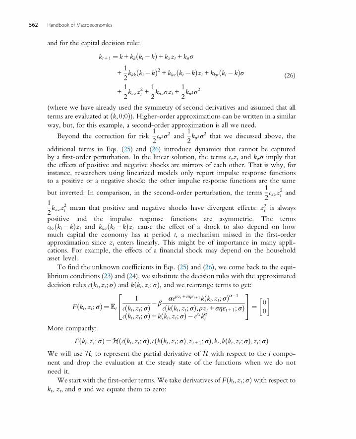
and for the capital decision rule:

kt+1 ¼ k+ kk kt�kð Þ+ kzzt + kσσ

+1

2kkk kt�kð Þ2 + kkz kt�kð Þzt + kkσ kt�kð Þσ

+1

2kzzz

2t +

1

2kσzσzt +

1

2kσ2σ

2

(26)

(where we have already used the symmetry of second derivatives and assumed that all

terms are evaluated at k,0;0ð Þ). Higher-order approximations can be written in a similar

way, but, for this example, a second-order approximation is all we need.

Beyond the correction for risk1

2cσ2σ

2 and1

2kσ2σ

2 that we discussed above, the

additional terms in Eqs. (25) and (26) introduce dynamics that cannot be capturedby a first-order perturbation. In the linear solution, the terms czzt and kσσ imply thatthe effects of positive and negative shocks are mirrors of each other. That is why, forinstance, researchers using linearized models only report impulse response functionsto a positive or a negative shock: the other impulse response functions are the same

but inverted. In comparison, in the second-order perturbation, the terms1

2czzz

2t and

1

2kzzz

2t mean that positive and negative shocks have divergent effects: z2t is always

positive and the impulse response functions are asymmetric. The termsckz kt�kð Þzt and kkz kt�kð Þzt cause the effect of a shock to also depend on howmuch capital the economy has at period t, a mechanism missed in the first-orderapproximation since zt enters linearly. This might be of importance in many appli-cations. For example, the effects of a financial shock may depend on the householdasset level.

To find the unknown coefficients in Eqs. (25) and (26), we come back to the equi-

librium conditions (23) and (24), we substitute the decision rules with the approximated

decision rules c kt,zt; σð Þ and k kt,zt; σð Þ, and we rearrange terms to get:

F kt,zt; σð Þ¼t

1

c kt,zt; σð Þ�βαeρzt + σηεt+1k kt ,zt; σð Þα�1

c k kt,zt; σð Þ,ρzt + σηεt+1; σð Þc kt,zt; σð Þ+ k kt,zt; σð Þ� ezt kαt

24

35¼ 0

0

�

More compactly:

F kt,zt; σð Þ¼H c kt,zt; σð Þ, c k kt,zt; σð Þ,zt+1; σð Þ,kt,k kt,zt; σð Þ,zt; σð ÞWe will use Hi to represent the partial derivative of H with respect to the i compo-

nent and drop the evaluation at the steady state of the functions when we do not

need it.

We start with the first-order terms. We take derivatives of F kt,zt; σð Þ with respect tokt, zt, and σ and we equate them to zero:


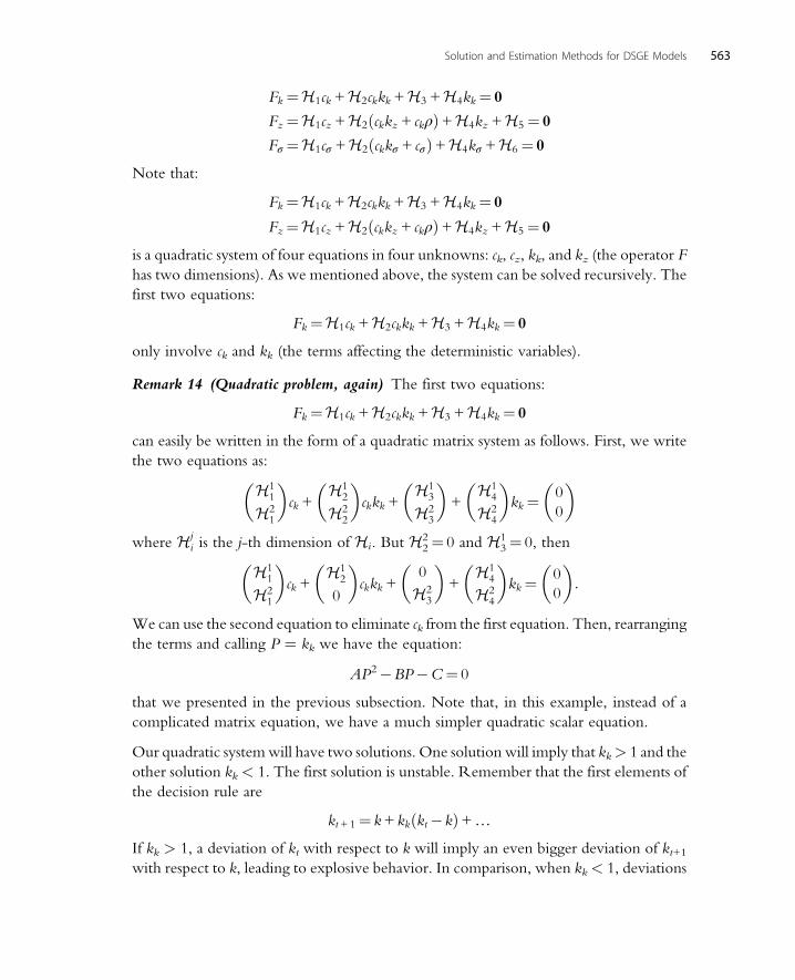
Fk ¼H1ck +H2ckkk +H3 +H4kk¼ 0

Fz¼H1cz +H2 ckkz + ckρð Þ+H4kz +H5 ¼ 0

Fσ ¼H1cσ +H2 ckkσ + cσð Þ+H4kσ +H6¼ 0

Note that:

Fk¼H1ck +H2ckkk +H3 +H4kk¼ 0

Fz¼H1cz +H2 ckkz + ckρð Þ+H4kz +H5¼ 0

is a quadratic system of four equations in four unknowns: ck, cz, kk, and kz (the operator F

has two dimensions). As we mentioned above, the system can be solved recursively. The

first two equations:


only involve ck and kk (the terms affecting the deterministic variables).

Remark 14 (Quadratic problem, again) The first two equations:


can easily be written in the form of a quadratic matrix system as follows. First, we write

the two equations as:

H11

H21

�ck +

H12

H22

�ckkk +

H13

H23

�+

H14

H24

�kk¼ 0

0

�

where Hji is the j-th dimension of Hi. But H2

2¼ 0 and H13¼ 0, then

H11

H21

�ck +

H12

0

�ckkk +

0

H23

�+

H14

H24

�kk¼ 0

0

�:

We can use the second equation to eliminate ck from the first equation. Then, rearranging

the terms and calling P ¼ kk we have the equation:

AP2�BP�C¼ 0

that we presented in the previous subsection. Note that, in this example, instead of a

complicated matrix equation, we have a much simpler quadratic scalar equation.

Our quadratic systemwill have two solutions. One solution will imply that kk> 1 and the

other solution kk < 1. The first solution is unstable. Remember that the first elements of

the decision rule are

kt+1¼ k+ kk kt�kð Þ+…

If kk > 1, a deviation of kt with respect to k will imply an even bigger deviation of kt+1with respect to k, leading to explosive behavior. In comparison, when kk < 1, deviations


of kt with respect to kwill, in the absence of additional shocks, dissipate over time. Once

we know ck and kk, we can come back to

Fz ¼H1cz +H2 ckkz + ckρð Þ+H4kz +H5¼ 0

and solve for cz and kz. As emphasized in Remark 12, this system is linear.

Finally, as in the general case, the last two equations

Fσ ¼H1cσ +H2 ckkσ + cσð Þ+H4kσ +H6¼ 0

form a linear, and homogeneous system in cσ and kσ. Hence, cσ ¼ kσ ¼ 0 and we obtain

the certainty equivalence of first-order approximations.

To find the second-order approximation, we take second derivatives of F kt,zt; σð Þaround k, 0, and 0:

Fkk¼ 0

Fkz¼ 0

Fkσ ¼ 0

Fzz¼ 0

Fzσ ¼ 0

Fσσ ¼ 0

(where we have already eliminated symmetric second derivatives). We substitute the

coefficients that we already know from the first-order approximation and we get a linear

system of 12 equations in 12 unknowns. Again, we get that all cross-terms on kσ and zσare zero.

Imposing the results concerning the coefficients that are equal to zero, we can rewrite

Eqs. (25) and (26) up to second-order as:

ct ¼ c + ck kt�kð Þ+ czzt

+1

2ckk kt�kð Þ2 + ckz kt�kð Þzt + 1

2czzz

2t +

1

2cσ2σ

2(27)

and

kt+1¼ k+ kk kt�kð Þ+ kzzt

+1

2kkk kt�kð Þ2 + kkz kt�kð Þzt + 1

2kzzz

2t +

1

2kσ2σ

2:(28)

Since even with this simple neoclassical growth model the previous systems of equations

are too involved to be written explicitly, we illustrate the procedure numerically. In

Table 1, we summarize the parameter values for the four parameters of the model.

We do not pretend to be selecting a realistic calibration (our choice of δ ¼ 1 precludes

any attempt at matching observed data). Instead, we pick standard parameter values in the


literature. The discount factor, β, is 0.99, the elasticity of output with respect to capital, α,is 0.33, the persistence of the autoregressive process, ρ, is 0.95, and the standard deviationof the innovation, η, is 0.01. With this calibration, the steady state is c ¼ 0.388 and

k ¼ 0.188.

The first-order components of the solution are (already selecting the stable solution):

ck¼ 0:680 cz ¼ 0:388kk¼ 0:330 kz¼ 0:188

and the second-order components:

ckk¼�2:420 ckz¼ 0:680 czz¼ 0:388 cσσ ¼ 0

kkk¼�1:174 kkz¼ 0:330 kzz¼ 0:188 kσσ ¼ 0

In addition, recall that we have the theoretical results: cσ ¼ kσ¼ ckσ ¼ kkσ ¼ czσ¼ kzσ¼ 0.

Thus, we get our second-order approximated solutions for the consumption decision

rule:

ct ¼ 0:388+ 0:680 kt�0:188ð Þ+0:388zt

�1:210 kt�0:188ð Þ2 + 0:680 kt�0:188ð Þzt +0:194z2t

and for the capital decision rule:

kt+1 ¼ 0:188+ 0:330 kt�0:188ð Þ+0:188zt

�0:587 kt�0:188ð Þ2 + 0:330 kt�0:188ð Þ zt +0:094z2t :

In this case, the correction for risk is zero. This should not be a surprise. In the neoclassical

growth model, risk is production risk driven by technology shocks. This production risk

is brought about by capital: the more capital the representative household accumulates,

the more it exposes itself to production risk. At the same time, the only asset available for

net saving in this economy is capital. Thus, any increment in risk (ie, a rise in the standard

deviation of the technology shock) generates two counterbalancing mechanisms: a desire

to accumulate more capital to buffer future negative shocks and a desire to accumulate less

capital to avoid the additional production risk. For low values of risk aversion, both

mechanisms nearly cancel each other (with a log utility function, they perfectly compen-

sate each other: in the exact solution, the standard deviation of the innovation to the

Table 1 CalibrationParameter Value

β 0.99

α 0.33

ρ 0.95

η 0.01


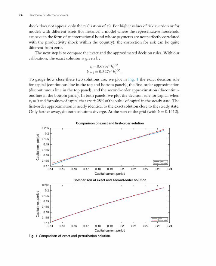
shock does not appear, only the realization of zt). For higher values of risk aversion or for

models with different assets (for instance, a model where the representative household

can save in the form of an international bond whose payments are not perfectly correlated

with the productivity shock within the country), the correction for risk can be quite

different from zero.

The next step is to compare the exact and the approximated decision rules. With our

calibration, the exact solution is given by:

ct ¼ 0:673eztk0:33t

kt+1¼ 0:327ezt k0:33t :

To gauge how close these two solutions are, we plot in Fig. 1 the exact decision rule

for capital (continuous line in the top and bottom panels), the first-order approximation

(discontinuous line in the top panel), and the second-order approximation (discontinu-

ous line in the bottom panel). In both panels, we plot the decision rule for capital when

zt¼ 0 and for values of capital that are 25% of the value of capital in the steady state. The

first-order approximation is nearly identical to the exact solution close to the steady state.

Only farther away, do both solutions diverge. At the start of the grid (with k ¼ 0.1412),

0.14 0.15 0.16 0.17 0.18 0.19 0.2 0.21 0.22 0.23 0.24

Capital current period

0.17

0.175

0.18

0.185

0.19

0.195

0.2

0.205

Cap

ital n

ext p

erio

d

Comparison of exact and first-order solution

ExactFirst-order

0.14 0.15 0.16 0.17 0.18 0.19 0.2 0.21 0.22 0.23 0.24

Capital current period

0.17

0.175

0.18

0.185

0.19

0.195

0.2

0.205

Cap

ital n

ext p

erio

d

Comparison of exact and second-order solution

ExactSecond-order

Fig. 1 Comparison of exact and perturbation solution.


the exact decision rule and the first-order approximation diverge by nearly 1%. The

second-order approximation, in comparison, is more accurate along the whole range

of values of capital. Even at k ¼ 0.1412, the difference between both solutions is only

0.13%. This result shows the often good global properties of perturbation solutions.

We will revisit below how to assess the accuracy of a solution. Suffice it to say at this

moment that whether 0.13% is too large or accurate enough is application dependent.

For instance, for the computation of business cycle moments, we often need less accuracy

than for welfare evaluations. The reason is that while errors in the approximation of a

moment of the model, such as the mean or variance of consumption, tend to cancel each

other, welfare is a nonlinear function of the allocation and small errors in computing an

allocation can translate into large errors in computing welfare.

4.4 PruningAlthough the higher-order perturbations that we described are intuitive and straightfor-

ward to compute, they often generate explosive sample paths evenwhen the corresponding

linear approximation is stable. These explosive sample paths arise because the higher-order

terms induce additional fixed points for the system, around which the approximated solu-

tion is unstable (see Kim et al., 2008 andDenHaan andDeWind, 2012). A simple example

clarifies this point. Imagine that we have an approximated decision rule for capital (where,

for simplicity, we have eliminated the persistence on the productivity process zt) that has

the form:

kt+1¼ a0 + a1kt + a2k2t +…+ b1εt +…

If we substitute recursively, we find:

kt+1¼ a1kt + a2 a1kt�1 + a2k2t�1

� �2+…+ b1εt +…,

an expression that involves terms in k3t�1 and k4t�1. If the support of εt is not bounded,sooner or later, we will have, in a simulation, an innovation large enough such that kt+1is far away from its steady-state value. As the simulation progresses over time, that value

of kt+1 will be raised to cubic and higher-order powers, and trigger an explosive path.

The presence of this explosive behavior complicates any model evaluation because no

unconditional moments would exist based on this approximation. It also means that

any unconditional moment-matching estimation methods, such as the generalized method

of moments (GMM) or the simulated method of moments (SMM), are inapplicable in

this context as they rely on finite moments from stationary and ergodic probability

distributions.

For second-order approximations, Kim et al. (2008) propose pruning the approxima-

tion. Loosely speaking, pruning means to eliminate, in the recursions, all terms that are of

a higher order than the order of the solution (ie, if we are dealing with a second-order


perturbation, all terms involving states or innovations raised to powers higher than 2).

Kim et al. (2008) prove that the pruned approximation does not explode.

Andreasen et al. (2013) extend Kim et al. (2008)’s approach by showing how to apply

pruning to an approximation of any arbitrary order by exploiting what the authors refer

to as the pruned state-space system. Under general technical conditions, Andreasen et al.

(2013) show that first and second unconditional moments for a pruned state-space system

exist. Then, they provide closed-form expressions for first and second unconditional

moments and impulse response functions. This is important because these expressions

let researchers avoid the use of numerical simulations to compute these moments. These

numerical simulations have often been shown to be unreliable, in particular, when solv-

ing for the generalized impulse response functions of DSGE models (for the definition of

generalized impulse response functions, see Koop et al., 1996). Andreasen et al. (2013)

also derive conditions for the existence of higher unconditional moments, such as

skewness and kurtosis.

4.5 Change of VariablesIn Remark 4, we discussed the possibility of performing the perturbation of a DSGE

model in logs of the variables of interest, instead of doing it in levels. In a creative

contribution, Judd (2003) argues that loglinearization is a particular case of the more

general idea of a change of variables and shows how this technique could be efficiently

implemented. In this subsection, we explain Judd’s contribution by following

Fernandez-Villaverde and Rubio-Ramırez (2006).

The point of departure is to note that if we have a Taylor expansion of a variable x

around a point a:

d xð Þ’ d að Þ+ @d að Þ@a

x� að Þ+H :O:T :,

(whereH.O.T. stands for higher-order terms), we can rewrite the expansion in terms of a

transformed variable Y xð Þ:

g yð Þ¼ h d X yð Þð Þð Þ¼ g bð Þ+ @g bð Þ@b

Y xð Þ� bð Þ+H :O:T :

where b¼Y að Þ and X yð Þ is the inverse of Y xð Þ. Since with a perturbation we find a

Taylor series approximation of the unknown function d that solves the operator H �ð Þas a function of the states x, the change of variables means we can find an alternative

Taylor series in terms of Y xð Þ.Why do we want to perform this change of variables? The famous British meteorol-

ogist Eric Eady (1915–1966) remarked once that: “It is not the process of linearization

that limits insight. It is the nature of the state that we choose to linearize about.”


By picking the right change of variables, we can reshape a highly nonlinear problem into

a much more linear one and, therefore, significantly increase the accuracy of the

perturbation.j

4.5.1 A Simple ExampleImagine that our aim is to approximate the decision rule for capital in our workhorse

stochastic neoclassical growth model with a first-order perturbation (the same ideas

would apply if we are trying to approximate other decision rules, expectations, value

functions, etc.). Remember that we derived that such an approximation had the form:

kt+1¼ k+ a1 kt�kð Þ+ b1zt

where a and b are the coefficients that we find by taking derivatives of F kt,zt; σð Þ and k

is the steady-state value of capital. In this section, it is more convenient to rewrite the

decision rule as:

kt+1�kð Þ¼ a1 kt�kð Þ+ b1zt:

Analogously a loglinear approximation of the policy function will take the form:

logkt+1� logk¼ a2 logkt� logkð Þ+ b2z

or in equivalent notation:

kt+1¼ a2kt + b2zt

where x¼ logx� logx0 is the percentage deviation of the variable x with respect to its

steady state.

How do we go from one approximation to the second one? First, we write the linear

system in levels as:

kt+1¼ dðkt,zt; σÞ¼ d k,0; 0ð Þ+ d1 k,0; 0ð Þ kt�kð Þ+ d2 k,0; 0ð Þztwhere d k,0; 0ð Þ¼ k, d1 k,0; 0ð Þ¼ a1, d2 k,0; 0ð Þ¼ b1. Second, we propose the changes of

variables h¼ logd, where Y xð Þ¼ logx and Y xð Þ¼ logx. Third, we apply Judd (2003)’s

formulae for this example:

logkt+1� logk¼ d1 k,0,0ð Þ logkt� logkð Þ+ 1

kd2 k,0,0ð Þz

Finally, by equating coefficients, we obtain a simple closed-form relation between the

parameters of both representations: a2 ¼ a1 and b2¼ 1

kb1:

j An idea related to the change of variables is the use of gauges, where the perturbation is undertaken not in

terms of powers of the perturbation parameter, σ, but of a series of gauge functions δn σð Þf g∞n¼1 such that:

lim n!∞δn+1 σð Þδn σð Þ ¼ 0: See Judd (1998) for details.


Three points are important. First, moving from a1 and b1 to a2 and b2 is an operation

that only involves k, a value that we already know from the computation of the first-order

perturbation in levels. Therefore, once the researcher has access to the linear solution,

obtaining the loglinear one is immediate.k Second, we have not used any assumption

on the utility or production functions except that they satisfy the general technical con-

ditions of the stochastic neoclassical growth model. Third, the change of variables can be

applied to a perturbation of an arbitrary order.We only presented the case for a first-order

approximation to keep the exposition succinct.

4.5.2 A More General CaseWe can now present a more general case of change of variables. The first-order solution

of a model is:

d xð Þ’ d að Þ+ @d að Þ@a

x� að Þ:

If we expand gðyÞ¼ h d X yð Þð Þð Þ around b¼Y að Þ, where X yð Þ is the inverse of Y xð Þ, wecan write:

g yð Þ¼ h d X yð Þð Þð Þ¼ g bð Þ+ gα bð Þ Yα xð Þ� bαð Þwhere gα¼ hAd

Ai X

iα comes from the application of the chain rule.

Following Judd (2003), we use this approach to encompass any power function

approximation of the form:

kt+1 k,z; γ,ζ,φð Þγ�kγ ¼ a3 kζt �kζ� �

+ b3zφ

where we impose φ� 1 to ensure that we have real values for the power zφ. Power func-

tions are attractive because, with only three free parameters γ,ζ,φð Þ, we can capture

many nonlinear structures and nest the log transformation as the limit case when the

coefficients γ and ζ tend to zero and φ ¼ 1. The changes of variables for this family

of functions are given by h ¼ dγ, Y ¼ xζ, and X ¼ y1ζ. Following the same reasoning

as before, we derive:

kt+1 k,z; γ,ζ,φð Þγ�kγ ¼ γ

ζkγ�ζa1 kζt �kζ

� �+

γ

φkγ�1b1z

φ:

The relation between the new and the old coefficients is again easy to compute:

a3¼ γ

ζkγ�ζa1 and b3¼ γ

φkγ�1b1.

k A heuristic argument that delivers the same result takes: kt +1�kð Þ¼ a1 kt�kð Þ+ b1zt and divides on both

sides by k:kt +1�k

k¼ a1

kt�k

k+1

kb1z:Noticing that

xt�x

x’ logxt� logx, we get back the same relation

as the one above. Our argument in the main text is more general and does not depend on an additional

approximation.


A slightly more restrictive case is to impose that γ ¼ ζ and z ¼ 1. Then, we get a

power function with only one free parameter γ:

kt+1 k,z; γð Þγ�kγ ¼ a4 kζt �kζ� �

+ b4z

or, by defining k�t ¼ k

γt �kγ, we get:

k�t+1¼ a4k

�t + b4z

with a4 ¼ a1 and b4 ¼ kγ�1b1. This representation has the enormous advantage of being a

linear system, which makes it suitable for analytic study and, as we will see in Section 10,

for estimation with a Kalman filter.

4.5.3 The Optimal Change of VariablesThe previous subsection showed how to go from a first-order approximation to the solu-

tion of a DSGEmodel to a more general representation indexed by some parameters. The

remaining question is how to select the optimal value of these parameters.l

Fernandez-Villaverde and Rubio-Ramırez (2006) argue that a reasonable criterion

(and part of the motivation for the change of variables) is to select these parameters to

improve the accuracy of the solution of the model. More concretely, the authors propose

to minimize the Euler error function with respect to some metric. Since we have not

introduced the measures of accuracy of the solution to a DSGE model, we will skip

the details of how to do so. Suffice it to say that Fernandez-Villaverde and Rubio-

Ramırez (2006) find that the optimal change of variables improves the average accuracy

of the solution by a factor of around three. This improvement makes a first-order approx-

imation competitive in terms of accuracy with much more involved methods.

Fernandez-Villaverde and Rubio-Ramırez (2006) also report that the optimal parameter

values depend on the standard deviation of the exogenous shocks to the economy. This is

a significant result: the change of variables corrects by the level of uncertainty existing in

the economy and breaks certainty equivalence.

Remark 15 (Loglinearization v. lognormal–loglinear approximation) A different solu-

tion technique, called lognormal–loglinear approximation, is popular in finance. Its rela-

tion with standard loglinearization (as a particular case of first-order perturbation with a

change of variables in logs) often causes confusion among researchers and students. Thus,

once we have understood the change of variables technique, it is worthwhile to dedicate

this remark to clarifying the similarities and differences between the first-order

l We do not even need to find the optimal value of these parameters. It may be the case that a direct but not

optimal choice of parameter values already delivers substantial improvements in accuracy at a very low

computational cost. When one is maximizing, for example, a likelihood function, being at the true

maximum matters. When one is finding parameters that improve accuracy, optimality is desirable but

not essential, and it can be traded off against computational cost.


perturbation in logs and the lognormal–loglinear approximation. The best way to illus-

trate this point is with a concrete example. Imagine that we have a household with utility

function

max0

X∞t¼0

βt logCt

and budget constraint:

Wt+1 ¼Rt+1 Wt�Ctð Þwhere Wt is total wealth and W0 is given. Then, the optimality conditions are:

1¼ βt

Ct

Ct+1

Rt+1

Wt+1 ¼Rt+1 Wt�Ctð Þ

with steady state R¼ 1

βand W ¼R W �Cð Þ:

Under a standard first-order perturbation in logs (loglinearization) around the

previous steady state, and after some algebra:

tΔct+1¼t r t+1

wt+1¼ r t+1 +1

ρwt + 1�1

ρ

�ct

where, for a variable Xt,

xt ¼ xt�x¼ logXt� logX

and ρ¼W �C

W. Subtracting wt from the second equation:

Δwt+1¼ r t+1 + 1�1

ρ

�ct� wtð Þ

If we want to express these two equations in logs, instead of log-deviations (and using the

fact that r ¼� logβ):

tΔct+1¼ logβ+trt+1 (29)

Δwt+1 ¼ rt+1 + k+ 1�1

ρ

�ct�wtð Þ (30)

where

k¼�r� 1�1

ρ

�c�wð Þ:


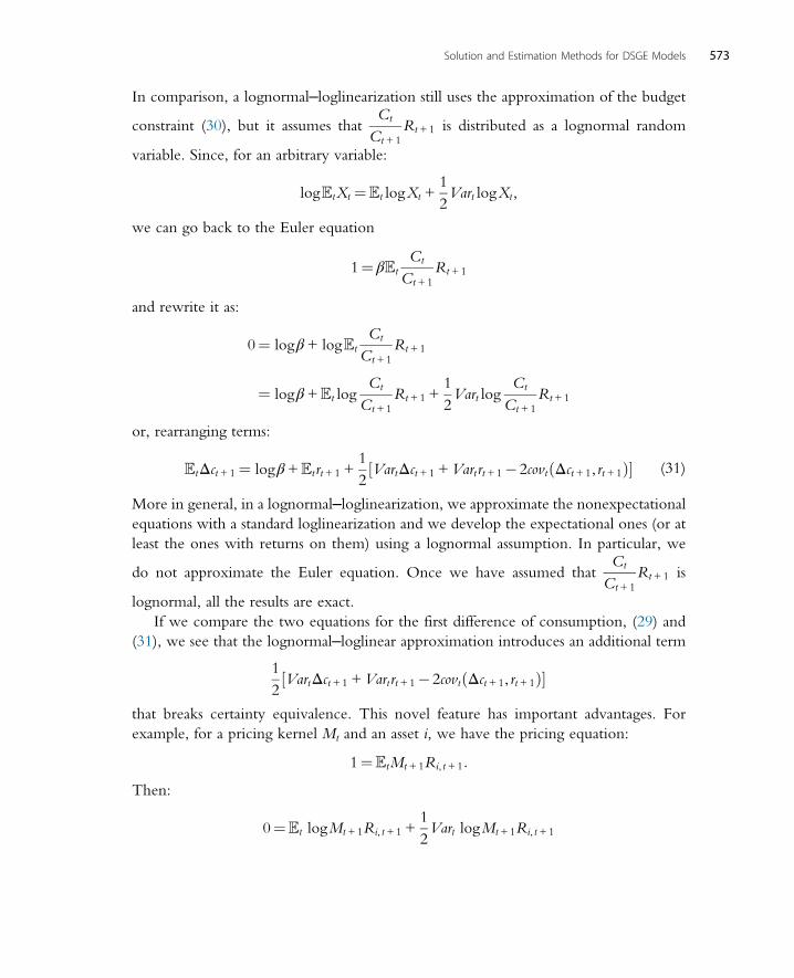
In comparison, a lognormal–loglinearization still uses the approximation of the budget

constraint (30), but it assumes thatCt

Ct+1

Rt+1 is distributed as a lognormal random

variable. Since, for an arbitrary variable:

logtXt ¼t logXt +1

2Vart logXt,

we can go back to the Euler equation

1¼ βt

Ct

Ct+1

Rt+1

and rewrite it as:

0¼ logβ+ logt

Ct

Ct+1

Rt+1

¼ logβ+t logCt

Ct+1

Rt+1 +1

2Vart log

Ct

Ct+1

Rt+1

or, rearranging terms:

tΔct+1¼ logβ+trt+1 +1

2VartΔct+1 +Vartrt+1�2covt Δct+1, rt+1ð Þ½ � (31)

More in general, in a lognormal–loglinearization, we approximate the nonexpectational

equations with a standard loglinearization and we develop the expectational ones (or at

least the ones with returns on them) using a lognormal assumption. In particular, we

do not approximate the Euler equation. Once we have assumed thatCt

Ct+1

Rt+1 is

lognormal, all the results are exact.

If we compare the two equations for the first difference of consumption, (29) and

(31), we see that the lognormal–loglinear approximation introduces an additional term

1

2VartΔct+1 +Vartrt+1�2covt Δct+1, rt+1ð Þ½ �

that breaks certainty equivalence. This novel feature has important advantages. For

example, for a pricing kernel Mt and an asset i, we have the pricing equation:

1¼tMt+1Ri, t+1:

Then:

0¼t logMt+1Ri, t+1 +1

2Vart logMt+1Ri, t+1


or:

t ri, t+1¼�tmt+1�1

2Vartmt+1�1

2Vartri, t+1� covt mt+1, ri, t+1ð Þ

If we look at the same expression for the risk-free bond:

1¼tMt+1Rf , t+1

we get:

rf , t+1¼�tmt+1�1

2Vartmt+1

and we can find that the excess return is:

t ri, t+1� rf , t+1¼�1

2Vartri, t+1� covt mt+1, ri, t+1ð Þ,

an expression that it is easy to interpret.

On the other hand, this expression also embodies several problems. First, it is often

unclear to what extent, in a general equilibrium economy,Ct

Ct+1

Rt+1 is close to lognor-

mality. Second, in lognormal–loglinear approximation, we are mixing two approaches, a

lognormal assumption with a loglinearization. This is not necessarily coherent from the

perspective of perturbation theory and we may lack theoretical foundations for the

approach (including an absence of convergence theorems). Third, in the loglinearization,

we can compute all the coefficients by solving a quadratic matrix system. In the

lognormal–loglinear approximation, we need to compute second moments and, in many

applications, how to do so may not be straightforward. Finally, it is not obvious how to

get higher-order approximations with the lognormal–loglinear approximation, while

perturbation theory can easily handle higher-order solutions.

4.6 Perturbing the Value FunctionIn some applications, it is necessary to perturb the value function of a DSGE model, for

example, when we are dealing with recursive preferences or when we want to evaluate

welfare. Furthermore, a perturbed value function can be an outstanding initial guess for

value function iteration, making it possible to deal with high-dimensional problems

that could be otherwise too slow to converge. Given the importance of perturbing

the value function, this section illustrates in some detail how to do so.

Since all that we learned in the general case subsection will still apply by just changing

the operator H from the equilibrium conditions to the Bellman operator, we can go

directly to a concrete application. Consider a value function problem (following the same

notation as above).


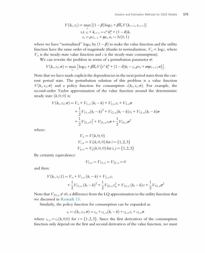
V kt,ztð Þ¼ maxct

1�βð Þ log ct + βtV kt+1,zt+1ð Þ½ �s:t: ct + kt+1¼ ezt kαt + 1�δð Þktzt ¼ ρzt�1 + ηεt, εt �N 0,1ð Þ

where we have “normalized” log ct by 1�βð Þ to make the value function and the utility

function have the same order of magnitude (thanks to normalization, Vss ¼ log c, where

Vss is the steady-state value function and c is the steady-state consumption).

We can rewrite the problem in terms of a perturbation parameter σ:

V kt,zt; σð Þ¼ maxct

log ct + βtV ezt kαt + 1�δð Þkt� ct,ρzt + σηεt+1; σ� ��

:

Note that we have made explicit the dependencies in the next period states from the cur-

rent period state. The perturbation solution of this problem is a value function

V kt,zt; σð Þ and a policy function for consumption c kt,zt; σð Þ. For example, the

second-order Taylor approximation of the value function around the deterministic

steady state k,0; 0ð Þ is:V kt,zt; σð Þ¼Vss +V1, ss kt�kð Þ+V2, sszt +V3, ssσ

+1

2V11, ss kt�kð Þ2 +V12, ss kt�kð Þzt +V13, ss kt�kð Þσ

+1

2V22, ssz

2t +V23, ssztσ +

1

2V33, ssσ

2

where:

Vss ¼V k,0; 0ð ÞVi, ss ¼Vi k,0; 0ð Þ for i¼ 1,2,3f gVij, ss ¼Vij k,0; 0ð Þ for i, j¼ 1,2,3f g

By certainty equivalence:

V3, ss ¼V13, ss¼V23, ss ¼ 0

and then:

V kt,zt;1ð Þ¼Vss +V1, ss kt�kð Þ+V2, sszt

+1

2V11, ss kt�kð Þ2 + 1

2V22, ssz

2tt +V12, ss kt�kð Þz+ 1

2V33, ssσ

2

Note thatV33,ss 6¼ s0, a difference from the LQ approximation to the utility function that

we discussed in Remark 13.

Similarly, the policy function for consumption can be expanded as:

ct ¼ c kt,zt; σð Þ¼ css + c1, ss kt�kð Þ+ c2, sszt + c3, ssσ

where ci, ss ¼ c1 k,0;0ð Þ for i¼ 1,2,3f g. Since the first derivatives of the consumption

function only depend on the first and second derivatives of the value function, we must


have that c3,ss ¼ 0 (remember that precautionary consumption depends on the third

derivative of the value function; Kimball, 1990).

To find the linear components of our approximation to the value function, we take

derivatives of the value function with respect to controls (ct), states (kt, zt), and the per-

turbation parameter σ and solve the associated system of equations when σ ¼ 0. We can

find the quadratic components of the value function by taking second derivatives,

plugging in the known components from the previous step, and solving the system

when σ ¼ 0.

We are ready now to show some of the advantages of perturbing the value function.

First, we have an evaluation of the welfare cost of business cycle fluctuations readily avail-

able. At the deterministic steady state kt ¼ k and zt ¼ 0, we have:

V k, 0; σð Þ¼Vss +1

2V33, ssσ

2:

Hence1

2V33, ssσ

2 is a measure of the welfare cost of the business cycle: it is the difference,

up to second-order, between the value function evaluated at the steady-state value of the

state variables k,0ð Þ and the steady-state value function (where not only are we at the

steady state, but where we know that in future periods we will be at that point as well).

Note that this last quantity is not necessarily negative. Indeed, it may well be positive in

many models, such as in a stochastic neoclassical growth model with leisure choice. For

an explanation and quantitative evidence, see Cho et al. (2015).m

It is easier to interpret V33,ss if we can transform it into consumption units. To do so,

we compute the decrease in consumption τ that will make the household indifferent

between consuming 1� τð Þc units per period with certainty or ct units with uncertainty.

That is, τ satisfies:

log 1� τð Þc¼ log c +1

2V33, ssσ

2

where we have used Vss¼ log c. Then,

τ¼ 1� e12V33, ssσ2 :

m In his classical calculation about the welfare cost of the business cycle, Lucas Jr. (1987) assumed an endow-

ment economy, where the representative household faces the same consumption process as the one

observed for the US economy. Thus, for any utility function with risk aversion, the welfare cost of the

business cycle must be positive (although Lucas’ point, of course, was that it was rather small). When

consumption and labor supply are endogenous, agents can take advantage of uncertainty to increase their

welfare. A direct utility function that is concave in allocations can generate a convex indirect utility

function on prices and those prices change in general equilibrium as a consequence of the agents’ responses

to uncertainty.


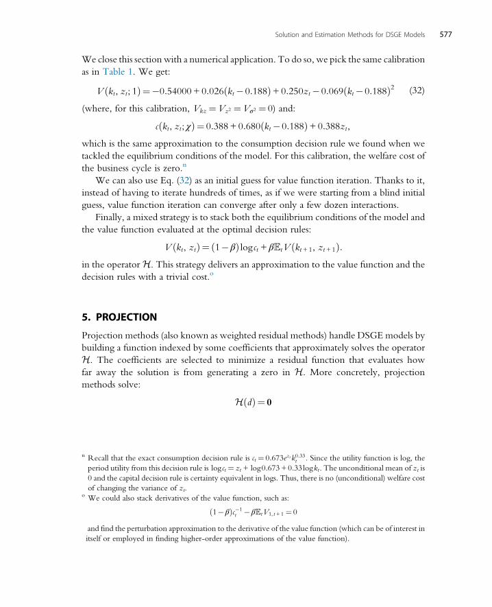
We close this section with a numerical application. To do so, we pick the same calibration

as in Table 1. We get:

V kt, zt; 1ð Þ¼�0:54000+ 0:026 kt�0:188ð Þ+0:250zt�0:069 kt�0:188ð Þ2 (32)

(where, for this calibration, Vkz¼Vz2 ¼Vσ2 ¼ 0) and:

c kt, zt; χð Þ¼ 0:388+ 0:680 kt�0:188ð Þ+0:388zt,

which is the same approximation to the consumption decision rule we found when we

tackled the equilibrium conditions of the model. For this calibration, the welfare cost of

the business cycle is zero.n

We can also use Eq. (32) as an initial guess for value function iteration. Thanks to it,

instead of having to iterate hundreds of times, as if we were starting from a blind initial

guess, value function iteration can converge after only a few dozen interactions.

Finally, a mixed strategy is to stack both the equilibrium conditions of the model and

the value function evaluated at the optimal decision rules:

V kt, ztð Þ¼ 1�βð Þ log ct + βtV kt+1, zt+1ð Þ:in the operatorH. This strategy delivers an approximation to the value function and the

decision rules with a trivial cost.o

5. PROJECTION

Projection methods (also known as weighted residual methods) handle DSGE models by

building a function indexed by some coefficients that approximately solves the operator

H. The coefficients are selected to minimize a residual function that evaluates how

far away the solution is from generating a zero in H. More concretely, projection

methods solve:

H dð Þ¼ 0

n Recall that the exact consumption decision rule is ct ¼ 0:673ezt k0:33t . Since the utility function is log, the

period utility from this decision rule is log ct ¼ zt + log0:673+ 0:33logkt. The unconditional mean of zt is

0 and the capital decision rule is certainty equivalent in logs. Thus, there is no (unconditional) welfare cost

of changing the variance of zt.o We could also stack derivatives of the value function, such as:

1�βð Þc�1t �βtV1, t +1 ¼ 0

and find the perturbation approximation to the derivative of the value function (which can be of interest in

itself or employed in finding higher-order approximations of the value function).


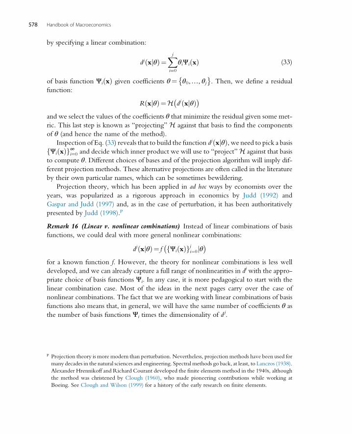
by specifying a linear combination:

dj xjθð Þ¼Xji¼0

θiΨi xð Þ (33)

of basis function Ψi xð Þ given coefficients θ¼ θ0,…, θj�

. Then, we define a residual

function:

R xjθð Þ¼H dj xjθð Þ� �and we select the values of the coefficients θ that minimize the residual given some met-

ric. This last step is known as “projecting” H against that basis to find the components

of θ (and hence the name of the method).

Inspection of Eq. (33) reveals that to build the function dj xjθð Þ, we need to pick a basisΨi xð Þf g∞i¼0 and decide which inner product we will use to “project”H against that basis

to compute θ. Different choices of bases and of the projection algorithm will imply dif-

ferent projection methods. These alternative projections are often called in the literature

by their own particular names, which can be sometimes bewildering.

Projection theory, which has been applied in ad hoc ways by economists over the

years, was popularized as a rigorous approach in economics by Judd (1992) and

Gaspar and Judd (1997) and, as in the case of perturbation, it has been authoritatively

presented by Judd (1998).p

Remark 16 (Linear v. nonlinear combinations) Instead of linear combinations of basis

functions, we could deal with more general nonlinear combinations:

dj xjθð Þ¼ f Ψi xð Þf gji¼0jθ� �

for a known function f. However, the theory for nonlinear combinations is less well

developed, and we can already capture a full range of nonlinearities in dj with the appro-

priate choice of basis functions Ψi. In any case, it is more pedagogical to start with the

linear combination case. Most of the ideas in the next pages carry over the case of

nonlinear combinations. The fact that we are working with linear combinations of basis

functions also means that, in general, we will have the same number of coefficients θ as

the number of basis functions Ψi times the dimensionality of dj.

p Projection theory is more modern than perturbation. Nevertheless, projection methods have been used for

many decades in the natural sciences and engineering. Spectral methods go back, at least, to Lanczos (1938).

Alexander Hrennikoff and Richard Courant developed the finite elements method in the 1940s, although

the method was christened by Clough (1960), who made pioneering contributions while working at

Boeing. See Clough and Wilson (1999) for a history of the early research on finite elements.


5.1 A Basic Projection AlgorithmConceptually, projection is easier to present than perturbation (although its computa-

tional implementation is harder). We can start directly by outlining a projection

algorithm:

Algorithm 1 (Projection Algorithm)

1. Define j + 1 known linearly independent functions ψ i :Ω!where j<∞. We call

the ψ0, ψ1,…, ψ j the basis functions. These basis functions depend on the vector of

state variables x.

2. Define a vector of coefficients θl ¼ [θ0l , θ1

l ,…, θjl] for l ¼ 1,…,m (where recall that m

is the dimension that the function d of interest maps into). Stack all coefficients on a

m �(j+1) matrix θ ¼ [θ1; θ2;…; θl].3. Define a combination of the basis functions and the θ’s:

dl, j � jθl� �¼Xji¼0

θliψ i �ð Þ

for l ¼ 1,…,m. Then:

d j � jθð Þ¼ d1, j � jθl� �; d2, j � jθl� �

;…; dm, j � jθl� �� :

4. Plug dj (�jθ) into the operator H(�) to find the residual equation:

R � jθð Þ¼H dj � jθð Þ� �:

5. Find the value of θ^that makes the residual equation as close to 0 as possible given

some objective function ρ : J2 � J2 ! :

θ ¼ arg minθ2m� j+1ð Þ

ρ R � jθð Þ,0ð Þ:

To ease notation, we have made two simplifications on the previous algorithm. First, we

assumed that, along each dimension of d, we used the same basis functions ψ i and the same

number j+1 of them.Nothing forces us to do so. At themere cost of cumbersome notation,

we could have different basis functions for each dimension and a different number of them

(ie, different j’s).While the former is not too common in practice, the latter is standard, since

some variables’ influence on the function d can be harder to approximate than others’.q

We specify a metric function ρ to gauge how close the residual function is to zero over

the domain of the state variables. For example, in Fig. 2, we plot two different residual

q For the nonlinear combination case, f Ψi xð Þf gji¼0jθ� �

, we would just write the residual function:

R � jθð Þ¼H f Ψi xð Þf gji¼0jθ� ��

and find the θ’s that minimize a given metric. Besides the possible computational complexities of dealing

with arbitrary functions f Ψi xð Þf gji¼0jθ� �

, the conceptual steps are the same.


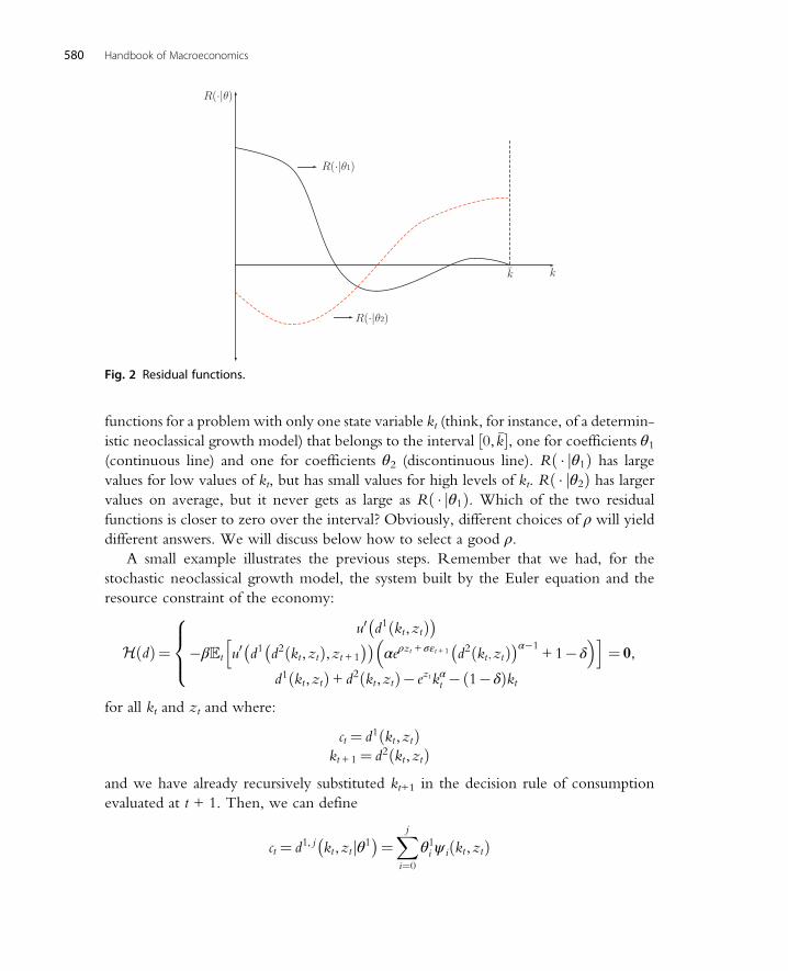
functions for a problem with only one state variable kt (think, for instance, of a determin-

istic neoclassical growth model) that belongs to the interval 0, �k½ �, one for coefficients θ1(continuous line) and one for coefficients θ2 (discontinuous line). R � jθ1ð Þ has large

values for low values of kt, but has small values for high levels of kt. R � jθ2ð Þ has largervalues on average, but it never gets as large as R � jθ1ð Þ. Which of the two residual

functions is closer to zero over the interval? Obviously, different choices of ρ will yield

different answers. We will discuss below how to select a good ρ.A small example illustrates the previous steps. Remember that we had, for the

stochastic neoclassical growth model, the system built by the Euler equation and the

resource constraint of the economy:

H dð Þ¼u0 d1 kt,ztð Þ� �

�βt u0 d1 d2 kt,ztð Þ,zt+1

� �� αeρzt + σεt+1 d2 kt ,ztð Þ� �α�1

+ 1�δ� �h i

d1 kt,ztð Þ+ d2 kt,ztð Þ� ezt kαt �ð1�δÞkt¼ 0

8><>: ,

for all kt and zt and where:

ct ¼ d1 kt,ztð Þkt+1 ¼ d2 kt,ztð Þ

and we have already recursively substituted kt+1 in the decision rule of consumption

evaluated at t + 1. Then, we can define

ct ¼ d1, j kt,ztjθ1� �¼Xj

i¼0

θ1i ψ i kt,ztð Þ

R(·|θ1)

R(·|θ)

k

R(·|θ2)

k

Fig. 2 Residual functions.


and

kt+1¼ d2, j kt,ztjθ2� �¼Xj

i¼0

θ2i ψ i kt,ztð Þ

for some ψ0 kt,ztð Þ,ψ1 kt,ztð Þ,…, ψ j kt,ztð Þ. Below we will discuss which basis functions

we can select for this role.

The next step is to write the residual function:

R kt,ztjθð Þ¼

u0Xj

i¼0θ1i ψ i kt,ztð Þ

� �

�βt

u0Xj

i¼0θ1i ψ i

Xj

i¼0θ2i ψn kt,ztð Þ,ρzt + σεt+1

� ��

� αeρzt + σεt+1

Xj

i¼0θ2i ψ i kt ,ztð Þ

� �α�1

+ 1�δ

�2664

3775

Pji¼0θ

1i ψ i kt,ztð Þ+

Xj

i¼0θ2i ψ i kt,ztð Þ� ezt kαt �ð1�δÞkt

8>>>>>>>>><>>>>>>>>>:

,

for all kt and zt, θ¼ θ1; θ2� �

.

The final step is to find θ¼ arg minθ2m� j+1ð Þρ R � jθð Þ,0ð Þ. Again, we will discuss

these choices below in detail, but just for concreteness, let us imagine that we pick m�j+1ð Þ points kl,zlð Þ and select the metric function to be zero at each of these m� j+1ð Þpoints and one everywhere else. Such a metric is trivially minimized if wemake the resid-

ual function equal to zero exactly on those points. This is equivalent to solving the system

of m� j+1ð Þ equations:R kl,zljθð Þ¼ 0, for l¼ 1,…,m� j+1ð Þ

with m� j+1ð Þ unknowns (we avoid here the discussion about the existence and

uniqueness of such a solution).

Remark 17 (Relation to econometrics) Many readers will be familiar with the use of the

word “projection” in econometrics. This is not a coincidence. A commonway to present

linear regression is to think about the problem of searching for the unknown conditional

expectation function:

Y jXð Þfor some variables Y and X. Given that this conditional expectation is unknown, we can

approximate it with the first twomonomials onX, 1 (a constant) andX (a linear function),

and associated coefficients θ0 and θ1:

Y jXð Þ’ θ0 + θ1X:

These two monomials are the first two elements of a basis composed by the monomials

(and also of the Chebyshev polynomials, a basis of choice later in this section). The

residual function is then:


R Y ,X jθ0,θ1ð Þ¼Y �θ0�θ1X :

The most common metric in statistical work is to minimize the square of this residual:

R Y ,X jθ0,θ1ð Þ2

by plugging in the observed series Y ,Xf gt¼1:T . The difference, thus, between ordi-

nary least squares and the projection algorithm is that while in the former we use

observed data, in the latter we use the operator H dð Þ imposed by economic theory.

This link is even clearer when we study the econometrics of semi-nonparametric

methods, such as sieves (Chen, 2007), which look for flexible basis functions indexed

by a low number of coefficients and that, nevertheless, impose fewer restrictions than

a linear regression.

Remark 18 (Comparison with other methods) From our short description of projection

methods, we can already see that other algorithms in economics are particular cases of it.

Think, for example, about the parameterized expectations approach (Marcet and

Lorenzoni, 1999). This approach consists of four steps.

First, the conditional expectations that appear in the equilibrium conditions of the

model are written as a flexible function of the state variables of the model and some coef-

ficients. Second, the coefficients are initialized at an arbitrary value. Third, the values of

the coefficients are updated by running a nonlinear regression that minimizes the distance

between the conditional expectations forecasted by the function guessed in step 1 and the

actual realization of the model along a sufficiently long simulation. Step 3 is repeated until

the coefficient values used to simulate the model and the coefficient values that come out

of the nonlinear regression are close enough.

Step 1 is the same as in any other projection method: the function of interest (in this

case the conditional expectation) is approximated by a flexible combination of basis func-

tions. Often the parameterized expectations approach relies on monomials to do so (or

functions of the monomials), which, as we will argue below, is rarely an optimal choice.

But this is not an inherent property of the approach. Christiano and Fisher (2000) propose

to use functions of Chebyshev polynomials, which will yield better results. More impor-

tant is the iterative procedure outlined by steps 2–4. Finding the fixed point of the values

of the coefficients by simulation and a quadratic distances is rarely the best option. Even if,

under certain technical conditions (Marcet and Marshall, 1994) the algorithm converges,

such convergence can be slow and fragile. In the main text, we will explain that a

collocation approach can achieve the same goal much more efficiently and without hav-

ing to resort to simulation (although there may be concrete cases where simulation is a

superior strategy).

Value function iteration and policy function iteration can also be understood as par-

ticular forms of projection, where the basis functions are linear functions (or higher-order


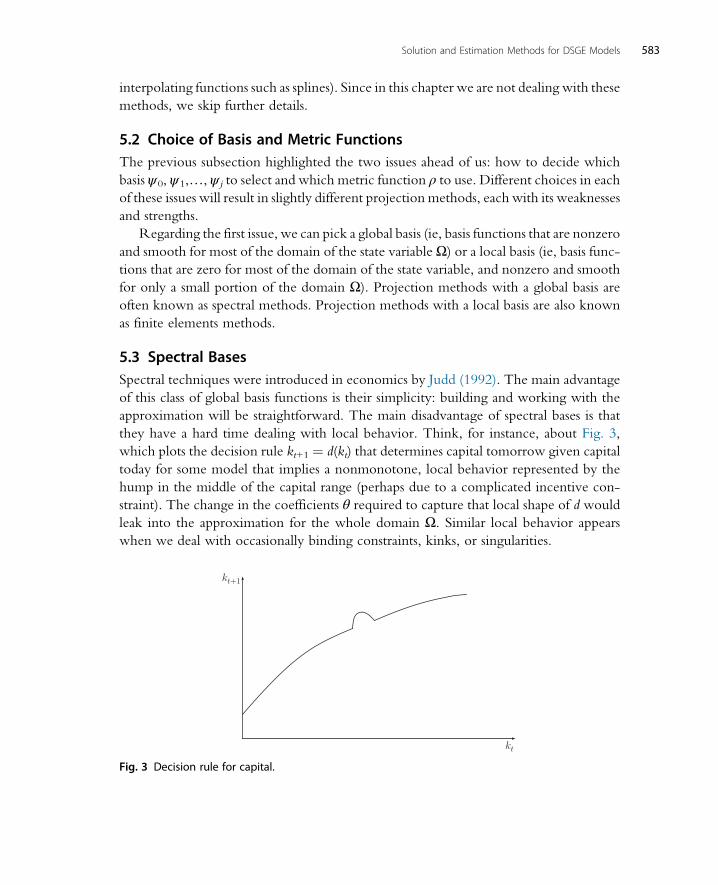
interpolating functions such as splines). Since in this chapter we are not dealing with these

methods, we skip further details.

5.2 Choice of Basis and Metric FunctionsThe previous subsection highlighted the two issues ahead of us: how to decide which

basis ψ0, ψ1,…, ψ j to select and which metric function ρ to use. Different choices in each

of these issues will result in slightly different projection methods, each with its weaknesses

and strengths.

Regarding the first issue, we can pick a global basis (ie, basis functions that are nonzero

and smooth for most of the domain of the state variable Ω) or a local basis (ie, basis func-tions that are zero for most of the domain of the state variable, and nonzero and smooth

for only a small portion of the domain Ω). Projection methods with a global basis are

often known as spectral methods. Projection methods with a local basis are also known

as finite elements methods.

5.3 Spectral BasesSpectral techniques were introduced in economics by Judd (1992). The main advantage

of this class of global basis functions is their simplicity: building and working with the

approximation will be straightforward. The main disadvantage of spectral bases is that

they have a hard time dealing with local behavior. Think, for instance, about Fig. 3,

which plots the decision rule kt+1 ¼ d(kt) that determines capital tomorrow given capital

today for some model that implies a nonmonotone, local behavior represented by the

hump in the middle of the capital range (perhaps due to a complicated incentive con-

straint). The change in the coefficients θ required to capture that local shape of d would

leak into the approximation for the whole domain Ω. Similar local behavior appears

when we deal with occasionally binding constraints, kinks, or singularities.

kt+1

kt

Fig. 3 Decision rule for capital.


A well-known example of this problem is the Gibbs phenomenon. Imagine that we

are trying to approximate a piecewise continuously differentiable periodic function with

a jump discontinuity, such as a square wave function (Fig. 4, panel A):

f xð Þ¼π

4, if x2 2jπ,2 j+1ð Þπ½ � and for 8j2

�π

4, otherwise:

8<:

Given that the function is periodic, a sensible choice for a basis is a trigonometric series

sin xð Þ, sin 2xð Þ, sin 3xð Þ, … The optimal approximation is:

sin xð Þ+ 1

3sin 3xð Þ+ 1

5sin 5xð Þ+…

The approximation behaves poorly at a jump discontinuity. As shown in Fig. 4, panel B,

even after using 10 terms, the approximation shows large fluctuations around all the

discontinuity points 2jπ and 2 j+1ð Þπ. These fluctuations will exist even if we keep add-ing many more terms to the approximation. In fact, the rate of convergence to the true

solution as n!∞ is only O nð Þ.

5.3.1 Unidimensional BasesWe will introduce in this subsection some of the most common spectral bases. First, we

will deal with the unidimensional case where there is only one state variable. This will

allow us to present most of the relevant information in a succinct fashion. It would be

important to remember, however, that our exposition of unidimensional bases cannot

be exhaustive (for instance, in the interest of space, we will skip splines) and that the

researcher may find herself tackling a problem that requires a specific basis. One of

the great advantages of projection methods is their flexibility to accommodate

Xt

Xt+

1

Square wave function

Xt

Xt+

1

10 Terms approximation

A B

Fig. 4 Gibbs phenomenon.


unexpected requirements. In the next subsection, we will deal with the case of an

arbitrary number of state variables and we will discuss how to address the biggest

challenge of projection methods: the curse of dimensionality.

5.3.1.1 MonomialsA first basis is the monomials 1, x, x2, x3, … Monomials are simple and intuitive. Fur-

thermore, even if this basis is not composed by orthogonal functions, if J1 is the space of

bounded measurable functions on a compact set, the Stone–Weierstrass theorem tells us

that we can uniformly approximate any continuous function defined on a closed interval

with linear combinations of these monomials.

Rudin (1976, p. 162) provides a formal statement of the theorem:

Theorem 1 (Stone–Weierstrass) LetA be an algebra of real continuous functions on a com-

pact setK. IfA separates points onK and ifA vanishes at no point ofK, then the uniform closure Bof A consists of all real continuous functions on K.

A consequence of this theorem is that if we have a real function f that is continuous onK,

we can find another function h2B such that for ε > 0:

f xð Þ�h xð Þj j< ε,

for all x 2 K.

Unfortunately, monomials suffer from two severe problems. First, monomials are

(nearly) multicollinear. Fig. 5 plots the graphs of x10 (continuous line) and x11 (discon-

tinuous line) for x2 0:5,1:5½ �. Both functions have a very similar shape. As we add higher

monomials, the new components of the solution do not allow the distance between the

exact function we want to approximate and the computed approximation to diminish

sufficiently fast.r

Second, monomials vary considerably in size, leading to scaling problems and the

accumulation of numerical errors. We can also see this point in Fig. 5: x11 goes from

4.8828e�04 to 86.4976 just by moving x from 0.5 to 1.5.

The challenges presented by the use of monomials motivate the search for an orthog-

onal basis in a natural inner product that has a bounded variation in range. Orthogonality

will imply that when we add more one element of the basis (ie, when we go from order j

r A sharp case of this problem is when H �ð Þ is linear. In that situation, the solution of the projection

involves the inversion of matrices. When the basis functions are similar, the condition numbers of these

matrices (the ratio of the largest and smallest absolute eigenvalues) are too high. Just the first six mono-

mials can generate condition numbers of 1010. In fact, the matrix of the least squares problem of fitting

a polynomial of degree 6 to a function (the Hilbert Matrix) is a popular test of numerical accuracy since

it maximizes rounding errors. The problem of the multicollinearity of monomials is also well appre-

ciated in econometrics.


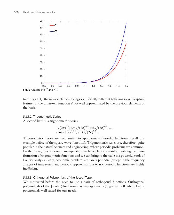
to order j + 1), the newest element brings a sufficiently different behavior so as to capture

features of the unknown function d not well approximated by the previous elements of

the basis.

5.3.1.2 Trigonometric SeriesA second basis is a trigonometric series

1= 2πð Þ0:5, cosx= 2πð Þ0:5, sinx= 2πð Þ0:5,…,

coskx= 2πð Þ0:5, sinkx= 2πð Þ0:5,…Trigonometric series are well suited to approximate periodic functions (recall our

example before of the square wave function). Trigonometric series are, therefore, quite

popular in the natural sciences and engineering, where periodic problems are common.

Furthermore, they are easy to manipulate as we have plenty of results involving the trans-

formation of trigonometric functions and we can bring to the table the powerful tools of

Fourier analysis. Sadly, economic problems are rarely periodic (except in the frequency

analysis of time series) and periodic approximations to nonperiodic functions are highly

inefficient.

5.3.1.3 Orthogonal Polynomials of the Jacobi TypeWe motivated before the need to use a basis of orthogonal functions. Orthogonal

polynomials of the Jacobi (also known as hypergeometric) type are a flexible class of

polynomials well suited for our needs.

Fig. 5 Graphs of x10 and x11.


The Jacobi polynomial of degree n, Pα,βn xð Þ for α, β > �1, is defined by the orthog-

onality condition:Z 1

�1

1�xð Þα 1+ xð ÞβPα,βn xð ÞPα,β

m xð Þdx¼ 0 form 6¼ n

One advantage of this class of polynomials is that we have a large number of alternative

expressions for them. The orthogonality condition implies, with the normalizations:

Pα,βn 1ð Þ¼ n+ α

n

�,

that the general n term is given by:

2�nXnk¼0

n+ αk

�n+ βn�k

�x�1ð Þn�k

x+1ð Þk

Recursively:

2 n+1ð Þ n+ α+ β+1ð Þ 2n+ α+ βð ÞPn+1¼2n+ α+ β+1ð Þ α2�β2

� �+ 2n+ α+ βð Þ 2n+ α+ β+1ð Þ 2n+ α+ β+2ð Þx

!Pn

�2 n+ αð Þ n+ βð Þ 2n+ α+ β+2ð ÞPn�1

Two important cases of Jacobi polynomials are the Legendre polynomials, where

α¼ β¼�1

2, and the Chebyshev polynomials, where α¼ β¼ 0. There is a generalization

of Legendre and Chebyshev polynomials, still within the Jacobi family, known as the

Gegenbauer polynomials, which set α¼ β¼ υ�1

2for a parameter υ.

Boyd and Petschek (2014) compare the performance of Gegenbauer, Legendre, and

Chebyshev polynomials. Their table 1 is particularly informative.We read it as suggesting

that, except for some exceptions that we find of less relevance in the solution of DSGE

models, Chebyshev polynomials are the most convenient of the three classes of polyno-

mials. Thus, from now on, we focus on Chebyshev polynomials.

5.3.1.4 Chebyshev PolynomialsChebyshev polynomials are one of the most common tools of applied mathematics. See,

for example, Boyd (2000) and Fornberg (1996) for references and background material.

The popularity of Chebyshev polynomials is easily explained if we consider some of their

advantages.

First, numerous simple closed-form expressions for the Chebyshev polynomials are

available. Thus, the researcher can easily move from one representation to another


according to her convenience. Second, the change between the coefficients of a Cheby-

shev expansion of a function and the values of the function at the Chebyshev nodes is

quickly performed by the cosine transform. Third, Chebyshev polynomials are more

robust than their alternatives for interpolation. Fourth, Chebyshev polynomials are

smooth and bounded between �1,1½ �. Finally, several theorems bound the errors for

Chebyshev polynomials’ interpolations.

The most common definition of the Chebyshev polynomials is recursive, with

T0 xð Þ¼ 1, T1 xð Þ¼ x, and the general n + 1-th order polynomial given by:

Tn+1 xð Þ¼ 2xTn xð Þ�Tn�1 xð ÞApplying this recursive definition, the first few polynomials are 1, x, 2x2 � 1, 4x3 � 3x,

8x4 � 8x2 + 1,… Thus, the approximation of a function with Chebyshev polynomials is

not different from an approximation with monomials (and, thus, we can rely on appro-

priate versions of the Stone–Weierstrass theorem), except that the orthogonality prop-

erties of how Chebyshev polynomials group the monomials make the approximation

better conditioned.

Fig. 6 plots the Chebyshev polynomials of order 0–5. The first two polynomials coin-

cide with the first two monomials, a constant and the 45-degree line. The Chebyshev

polynomial of order two is a parabola. Higher-order Chebyshev polynomials accumulate

several waves. Fig. 6 shows that the Chebyshev polynomials of order n has n zeros,

given by

xk¼ cos2k�1

2nπ

�,k¼ 1,…,n:

This property will be useful when we describe collocation in a few pages. Also, these

zeros are quadratically clustered toward 1.

Other explicit and equivalent definitions for the Chebyshev polynomials include

Tn xð Þ¼ cos n arccos xð Þ

¼ 1

2zn +

1

zn

�where

1

2z+

1

z

�¼ x

¼ 1

2x+ x2�1� �0:5� �n

+ x� x2�1� �0:5� �n� �

¼ 1

2

Xn=2½ �

k¼0

�1ð Þk n�k�1ð Þ!k! n�2kð Þ! 2xð Þn�2k

¼ �1ð Þnπ0:5

2nΓ n+1

2

� 1�x2� �0:5 dn

dxn1�x2� �n� 1

2

�:


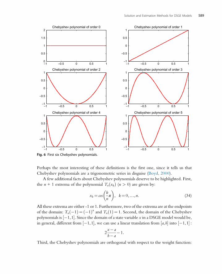
Perhaps the most interesting of these definitions is the first one, since it tells us that

Chebyshev polynomials are a trigonometric series in disguise (Boyd, 2000).

A few additional facts about Chebyshev polynomials deserve to be highlighted. First,

the n + 1 extrema of the polynomial Tn xkð Þ (n > 0) are given by:

xk¼ cosk

nπ

�, k¼ 0,…,n: (34)

All these extrema are either -1 or 1. Furthermore, two of the extrema are at the endpoints

of the domain: Tn �1ð Þ¼ �1ð Þn and Tn 1ð Þ¼ 1. Second, the domain of the Chebyshev

polynomials is �1,1½ �. Since the domain of a state variable x in a DSGE model would be,

in general, different from �1,1½ �, we can use a linear translation from a,b½ � into �1,1½ � :2x� a

b� a�1:

Third, the Chebyshev polynomials are orthogonal with respect to the weight function:

–1 –0.5 0 0.5 10

0.5

1

1.5

2Chebyshev polynomial of order 0

–1 –0.5 0 0.5 1–1

–0.5

0

0.5


–1 –0.5 0 0.5 1–1

–0.5

0

0.5


–1 –0.5 0 0.5 1–1

–0.5

0

0.5


–1 –0.5 0 0.5 1–1

–0.5

0

0.5


–1 –0.5 0 0.5 1–1

–0.5

0

0.5


Fig. 6 First six Chebyshev polynomials.


w xð Þ¼ 1

1�x2ð Þ0:5 :

We conclude the presentation of Chebyshev polynomials with two remarkable results,

which we will use below. The first result, due to Erd€os and Turan (1937),s tells us

that if an approximating function is exact at the roots of the nth1 order Chebyshev

polynomial, then, as n1!∞, the approximation error becomes arbitrarily small.

The Chebyshev interpolation theorem will motivate, in a few pages, the use of orthogonal

collocation where we pick as collocation points the zeros of a Chebyshev polynomial

(there are also related, less used, results when the extrema of the polynomials are

chosen instead of the zeros).

Theorem 2 (Chebyshev interpolation theorem) If d xð Þ 2 C a,b½ �, if ϕi xð Þ,fi¼ 0,…g is a system of polynomials (where ϕi xð Þ is of exact degree i) orthogonal to with respectto w xð Þ on a,b½ � and if pj ¼

Pji¼0 θiϕi xð Þ interpolates f xð Þ in the zeros of ϕn+1 xð Þ, then:

limj!∞

d� pj��

2

� �2¼ lim

n!∞

Z b

a

w xð Þ d xð Þ� pj� �2

dx¼ 0

We stated a version of the theorem that shows L2 convergence (a natural norm in eco-

nomics), but the result holds for Lp convergence for any p > 1. Even if we called this

result the Chebyshev interpolation theorem, its statement is more general, as it will

apply to other polynomials that satisfy an orthogonality condition. The reason we used

Chebyshev in the theorem’s name is that the results are even stronger if the function d xð Þsatisfies a Dini–Lipschitz condition and the polynomials ϕi xð Þ are Chebyshev to uniformconvergence, a much more reassuring finding.t

But the previous result requires that j!∞, which is impossible in real applications.

The second result will give a sense of how big is the error we are accepting by truncating

the approximation of d �ð Þ after a finite (and often relatively low) j.

s We reproduce the statement of the theorem, with only minor notational changes, from Mason and

Handscomb (2003), chapter 3, where the interested reader can find related results and all the relevant

details. This class of theorems is usually derived in the context of interpolating functions.t A function f satisfies a Dini–Lipschitz condition if

limδ!0+

ω δð Þ logδ¼ 0

where ω δð Þ is a modulus of continuity of f with respect to δ such that:

f x+ δð Þ� f xð Þj j �ω δð Þ:


Theorem 3 (Chebyshev truncation theorem, Boyd (Boyd (2000), p. 47)) The

error in approximating d is bounded by the sum of the absolute values of all the neglected coefficients.

In other words, if we have

dj � jθð Þ¼Xji¼0

θiψ i �ð Þ

then

d xð Þ� dj xjθð Þ�� X∞i¼j+1

θij j

for any x2 �1,1½ � and any j.We can make the last result even stronger. Under certain technical conditions, we will

have a geometric convergence of the Chebyshev approximation to the exact unknown

function.u And when we have geometric convergence,

d xð Þ� dj xjθð Þ�� O θj� �

that is, the truncation error created by stopping at the polynomial j is of the same order of

magnitude as the coefficient θj of the last polynomial. This result also provides us with a

simple numerical test: we can check the coefficient θj from our approximation: if θj is notclose enough to zero, we probably need to increase j. We will revisit the evaluation of the

accuracy of an approximation in Section 7.

Remark 19 (Change of variables) Wementioned above that, since a state variable xt in a

DSGEmodel would have, in general, a domain different from �1,1½ �, we can use a lineartranslation from a,b½ � into �1,1½ � :

2xt� a

b� a�1:

This transformation points to a more general idea: the change of variables as a way to

improve the accuracy of an approximation (see also Section 4.5 for the application of

the same idea in perturbation). Imagine that we are solving the stochastic neoclassical

growth model. Instead of searching for

ct ¼ d1 kt,ztð Þand

kt+1¼ d2 kt,ztð Þ,

u Convergence of the coefficients is geometric if lim j!∞ log θj��

=j¼ constant: If the lim is infinity, con-

vergence is supergeometric; if the lim is zero, convergence is subgeometric.


we could, instead, search for

log ct ¼ d1 logkt, ztð Þand

logkt+1¼ d2 logkt, ztð Þ,by defining

log ct ¼ d1, j logkt, ztjθ1� �¼Xj

i¼0

θ1i ψ i logkt, ztð Þ

and

logkt+1 ¼ d2, j logkt, ztjθ2� �¼Xj

i¼0

θ2i ψ i logkt, ztð Þ:

In fact, even in the basic projection example above, we already have a taste of this idea, as

we used zt as a state variable, despite the fact that it appears in the production function

as ezt . An alternative yet equivalent reparameterization writes At ¼ ezt and zt ¼ logAt.

The researcher can use her a priori knowledge of the model (or preliminary computa-

tional results) to search for an appropriate change of variables in her problem. We have

changed both state and control variables, but nothing forced us to do so: we could

have just changed one variable but not the other or employed different changes of

variables.

Remark 20 (Boyd’s moral principle)

All of the conveniences of Chebyshev polynomials we just presented are not just theo-

retical. Decades of real-life applications have repeatedly shown how well Chebyshev

polynomials work in a wide variety of applications. In the case of DSGEmodels, the out-

standing performance of Chebyshev polynomial has been shown by Aruoba et al. (2006)

and Caldara et al. (2012). Boyd (2000, p. 10), only half-jokingly, has summarized these

decades of experience in what he has named his Moral Principle 1:

1. When in doubt, use Chebyshev polynomials unless the solution is spatially periodic,

in which case an ordinary Fourier series is better.

2. Unless you are sure another set of basis functions is better, use Chebyshev

polynomials.

3. Unless you are really, really sure another set of basis functions is better, use Chebyshev

polynomials.

5.3.2 Multidimensional BasesAll of the previous discussion presented unidimensional basis functions. This was useful to

introduce the topic. However, most problems in economics are multidimensional: nearly


all DSGE models involve several state variables. How do we generalize our basis

functions?

The answer to this question is surprisingly important. Projection methods suffer from

an acute curse of dimensionality. While solving DSGE models with one or two state

variables and projection methods is relatively straightforward, solving DSGE models

with 20 state variables and projection methods is a challenging task due to the curse

of dimensionality. The key to tackling this class of problems is to intelligently select

the multidimensional basis.

5.3.2.1 Discrete State VariablesThe idea that the state variables are continuous was implicit in our previous discussion.

However, there are many DSGE models where either some state variable is discrete

(ie, the government can be in default or not, as in Bocola (2015), or monetary policy

can be either active or passive in the sense of Leeper, 1991) or where we can discretize

one continuous state variable without losing much accuracy. The best example of the

latter is the discretization of exogenous stochastic processes for productivity or preference

shocks. Such discretization can be done with the procedures proposed by Tauchen

(1986) or Kopecky and Suen (2010), who find a finite state Markov chain that generates

the same population moments as the continuous process. Experience suggests that, in

most applications, a Markov chain with 5 or 7 states suffices to capture nearly all the

implications of the stochastic process for quantitative analysis.

A problemwith discrete state variables can be thought of as one where we search for a

different decision rule for each value of that state variable. For instance, in the stochastic

neoclassical growthmodel with state variables kt and zt, we can discretize the productivity

level zt into a Markov chain with n points

zt 2 z1, ::,znf gand transition matrix:

Pz,z0 ¼p11 … p1n

..

.€ ..

.

pn1 … pnn

8><>:

9>=>; (35)

where entry pij is the probability that the chain will move from position i in the current

period to position j in the next period.

Remark 21 (Discretization methods) Tauchen (1986) procedure to discretize an AR(1)

stochastic process

zt ¼ ρzt�1 + Et

with stationary distribution Nð0,σ2zÞ, where σz ¼σEffiffiffiffiffiffiffiffiffiffiffiffi1�ρ2

p , works as follows:


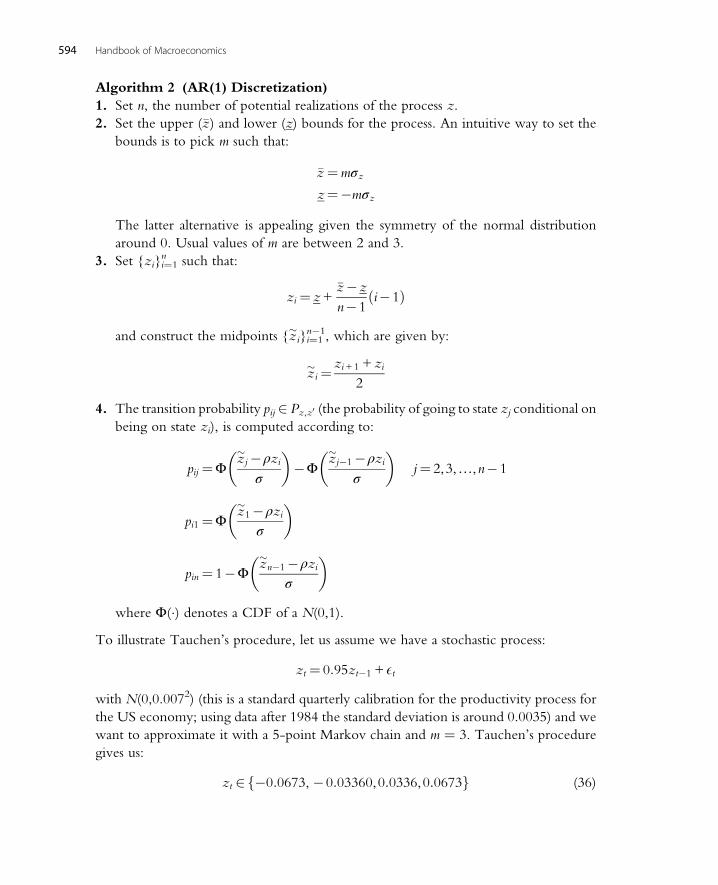
Algorithm 2 (AR(1) Discretization)

1. Set n, the number of potential realizations of the process z.

2. Set the upper (�z) and lower (z) bounds for the process. An intuitive way to set the

bounds is to pick m such that:

�z¼mσz

z¼�mσz

The latter alternative is appealing given the symmetry of the normal distribution

around 0. Usual values of m are between 2 and 3.

3. Set {zi}i¼1n such that:

zi ¼ z+�z�z

n�1ði�1Þ

and construct the midpoints {z�i}i¼1n�1, which are given by:

z�i¼ zi+1 + zi

2

4. The transition probability pij2 Pz,z0 (the probability of going to state zj conditional on

being on state zi), is computed according to:

pij ¼Φz�j�ρziσ

��Φ

z�j�1�ρzi

σ

�j¼ 2,3,…,n�1

pi1¼Φz�1�ρziσ

�

pin ¼ 1�Φz�n�1�ρzi

σ

�

where Φ(�) denotes a CDF of a N(0,1).

To illustrate Tauchen’s procedure, let us assume we have a stochastic process:

zt ¼ 0:95zt�1 + Et

with N(0,0.0072) (this is a standard quarterly calibration for the productivity process for

the US economy; using data after 1984 the standard deviation is around 0.0035) and we

want to approximate it with a 5-point Markov chain and m ¼ 3. Tauchen’s procedure

gives us:

zt 2 �0:0673, �0:03360,0:0336,0:0673f g (36)


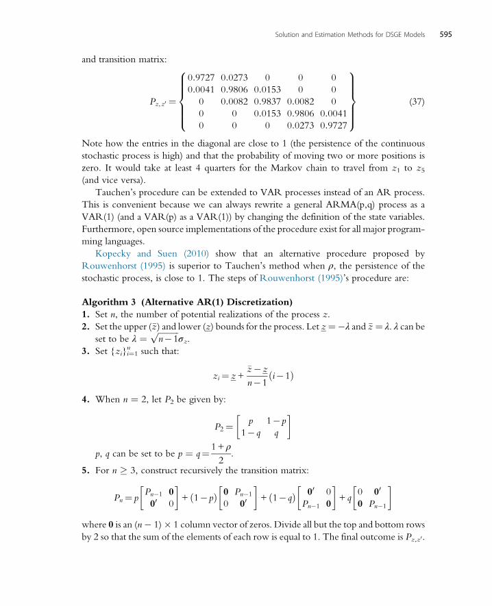
and transition matrix:

Pz,z0 ¼

0:9727 0:0273 0 0 0

0:0041 0:9806 0:0153 0 0

0 0:0082 0:9837 0:0082 0

0 0 0:0153 0:9806 0:00410 0 0 0:0273 0:9727

8>>>><>>>>:

9>>>>=>>>>;

(37)

Note how the entries in the diagonal are close to 1 (the persistence of the continuous

stochastic process is high) and that the probability of moving two or more positions is

zero. It would take at least 4 quarters for the Markov chain to travel from z1 to z5(and vice versa).

Tauchen’s procedure can be extended to VAR processes instead of an AR process.

This is convenient because we can always rewrite a general ARMA(p,q) process as a

VAR(1) (and a VAR(p) as a VAR(1)) by changing the definition of the state variables.

Furthermore, open source implementations of the procedure exist for all major program-

ming languages.

Kopecky and Suen (2010) show that an alternative procedure proposed by

Rouwenhorst (1995) is superior to Tauchen’s method when ρ, the persistence of the

stochastic process, is close to 1. The steps of Rouwenhorst (1995)’s procedure are:

Algorithm 3 (Alternative AR(1) Discretization)

1. Set n, the number of potential realizations of the process z.

2. Set the upper (�z) and lower (z) bounds for the process. Let z¼�λ and �z ¼ λ. λ can beset to be λ ¼ ffiffiffiffiffiffiffiffiffiffi

n�1p

σz.3. Set {zi}i¼1

n such that:

zi¼ z+�z�z

n�1ði�1Þ

4. When n ¼ 2, let P2 be given by:

P2¼ p 1�p

1� q q

�

p, q can be set to be p ¼ q¼ 1+ ρ

2.

5. For n � 3, construct recursively the transition matrix:

Pn¼ pPn�1 0

00 0

� + ð1�pÞ 0 Pn�1

0 00

� + ð1� qÞ 00 0

Pn�1 0

� + q

0 00

0 Pn�1

�

where 0 is an (n� 1)� 1 column vector of zeros. Divide all but the top and bottom rows

by 2 so that the sum of the elements of each row is equal to 1. The final outcome is Pz,z0.


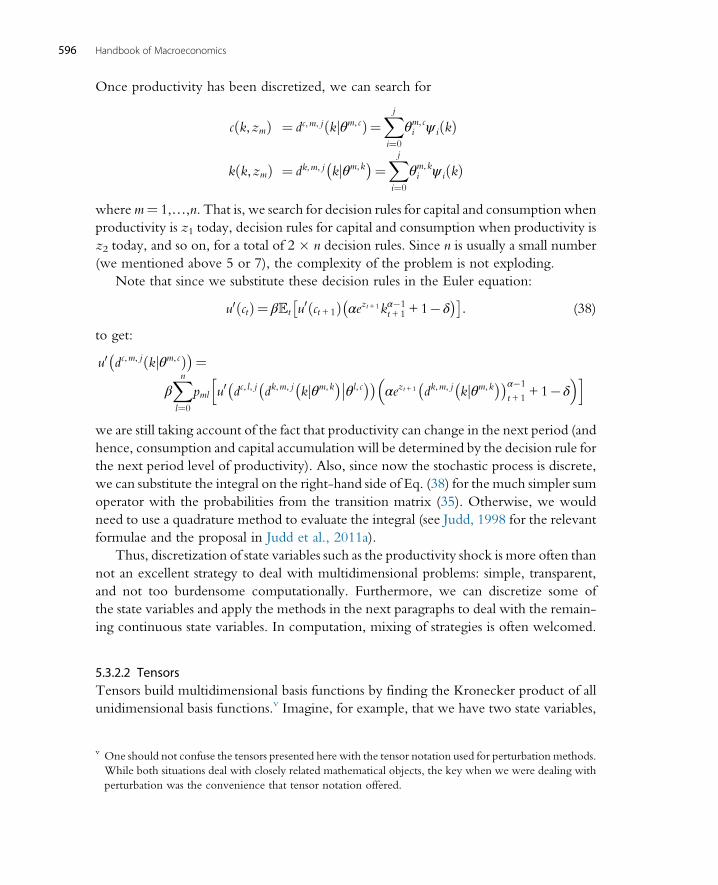
Once productivity has been discretized, we can search for

c k,zmð Þ ¼ dc,m, j kjθm, cð Þ¼Xji¼0

θm, ci ψ i kð Þ

k k,zmð Þ ¼ dk,m, j kjθm,k� �¼Xji¼0

θm,ki ψ i kð Þ

wherem¼ 1,…,n. That is, we search for decision rules for capital and consumption when

productivity is z1 today, decision rules for capital and consumption when productivity is

z2 today, and so on, for a total of 2 � n decision rules. Since n is usually a small number

(we mentioned above 5 or 7), the complexity of the problem is not exploding.

Note that since we substitute these decision rules in the Euler equation:

u0 ctð Þ¼ βt u0 ct+1ð Þ αezt +1kα�1

t+1 + 1�δ� ��

: (38)

to get:

u0 dc,m, j kjθm, cð Þ� �¼βXnl¼0

pml u0 dc, l, j dk,m, j kjθm,k� ��θl, c� ��

αezt+1 dk,m, j kjθm,k� �� α�1

t+1+ 1�δ

� �h i

we are still taking account of the fact that productivity can change in the next period (and

hence, consumption and capital accumulation will be determined by the decision rule for

the next period level of productivity). Also, since now the stochastic process is discrete,

we can substitute the integral on the right-hand side of Eq. (38) for the much simpler sum

operator with the probabilities from the transition matrix (35). Otherwise, we would

need to use a quadrature method to evaluate the integral (see Judd, 1998 for the relevant

formulae and the proposal in Judd et al., 2011a).

Thus, discretization of state variables such as the productivity shock is more often than

not an excellent strategy to deal with multidimensional problems: simple, transparent,

and not too burdensome computationally. Furthermore, we can discretize some of

the state variables and apply the methods in the next paragraphs to deal with the remain-

ing continuous state variables. In computation, mixing of strategies is often welcomed.

5.3.2.2 TensorsTensors build multidimensional basis functions by finding the Kronecker product of all

unidimensional basis functions.v Imagine, for example, that we have two state variables,

v One should not confuse the tensors presented here with the tensor notation used for perturbation methods.

While both situations deal with closely related mathematical objects, the key when we were dealing with

perturbation was the convenience that tensor notation offered.


physical capital kt and human capital ht. We have three Chebyshev polynomials for each

of these two state variables:

ψk0 ktð Þ, ψk

1 ktð Þ, and ψk2 ktð Þ

and

ψh0 htð Þ, ψh

1 htð Þ, and ψh2 htð Þ:

Then, the tensor is given by:

ψk0 ktð Þψh

0 htð Þ,ψk0 ktð Þψh







1 htð Þ, and ψk2 ktð Þψh

2 htð Þ:More formally, imagine that we want to approximate a function of n state variables

d : ½�1,1�n! with Chebyshev polynomial of degree j. We build the sum:

dj � jθð Þ¼Xji1¼0

…

Xjin¼0

θi1,…, inψ1i1

�ð Þ*…*ψnin

�ð Þ

where ψκiκis the Chebyshev polynomials of degree iκ on the state variable κ and θ is the

vector of coefficients θi1,…, in . To make the presentation concise, we have made three

simplifying assumptions. First, we are dealing with the case that d is one dimensional.

Second, we are using the same number of Chebyshev polynomials for each state variable.

Three, the functions ψκiκcould be different from the Chebyshev polynomials and

belong to any basis we want (there can even be a different basis for each state variable).

Eliminating these simplifications is straightforward, but notationally cumbersome.

There are two main advantages of a tensor basis. First, it is trivial to build. Second, if

the one-dimensional basis is orthogonal, then the tensor basis is orthogonal in the product

norm. The main disadvantage is the exponential growth in the number of coefficients

θi1,…, in : (j+1)n. In the example above, even using only three Chebyshev polynomials

(ie, j ¼ 2) for each of these two state variables, we end up having to solve for nine

coefficients. This curse of dimensionality is acute: with five state variables and three

Chebyshev polynomials, we end up with 243 coefficients. With ten Chebyshev polyno-

mials, we end up with 100,000 coefficients.

5.3.2.3 Complete PolynomialsIn practice, it is infeasible to use tensors when we are dealing with models with more than

3 continuous state variables and a moderate j. A solution is to eliminate some elements of

the tensor in a way that avoids much numerical degradation. In particular, Gaspar and

Judd (1997) propose using the complete polynomials:

Pnκ ψ1

i1*…*ψn

inwith jij � κ

n o


where

jij ¼Xnl¼1

il, 0� i1,…, in:

Completepolynomials, insteadof employing all the elements of the tensor, keeponly those

such that the sumof the order of the basis functions is less than a prefixed κ. The intuition isthat the elements of the tensor ψ1

i1*…*ψn

in, jij> κ add little additional information to the

basis: most of the flexibility required to capture the behavior of d is already in the complete

polynomials. For instance, if we are dealing with three state variables and Chebyshev

polynomials j ¼ 4, we can keep the complete polynomials of order 6:

P36 ψ1

i1*…*ψn

inwith jij � 6

n o:

Complete polynomials eliminate many coefficients: in our example, instead of (4 + 1)3¼125 coefficients of the tensor, when κ ¼ 6 we only need to approximate 87 coefficients.

Unfortunately,we still need toomany coefficients. In Section 5.7,wewill present an alter-

native: Smolyak’s algorithm.However, since themethod requires the introductionof a fair

amount of new notation and the presentation of the notion of interpolating polynomials,

we postpone the discussion and, instead, start analyzing the finite element methods.

5.4 Finite ElementsFinite elements techniques, based on local basis functions, were popularized in econom-

ics by McGrattan (1996) (see, also, Hughes (2000), for more background, and Brenner

and Scott (2008), for all the mathematical details that we are forced to skip in a handbook

chapter). The main advantage of this class of basis functions is they can easily capture local

behavior and achieve a tremendous level of accuracy even in the most challenging prob-

lems. That is why finite element methods are often used in mission-critical design in

industry, such as in aerospace or nuclear power plant engineering. Themain disadvantage

of finite elements methods is that they are hard to code and expensive to compute.

Therefore, we should choose this strategy when accuracy is more important than speed

of computation or when we are dealing with complicated, irregular problems.

Finite elements start by bounding the domain Ω of the state variables. Some of the

bounds would be natural (ie, kt > 0). Other bounds are not (kt < �k) and we need some

care in picking them. For example, we can guess a �k sufficiently large such that, in the

simulations of the model, kt never reaches �k. This needs, however, to be verified and

some iterative fine-tuning may be required.w

w Even if the simulation rarely reaches �k, it may be useful to repeat the computation with a slightly higher

bound ω�k, with ω > 1, to check that we still do not get to �k. In some rare cases, the first simulation might

not have reached �k because the approximation of the function d �ð Þ precluded traveling into that region.


The second step in the finite elements method is to partition Ω into small, noninter-

secting elements. These small sections are called elements (hence the name, “finite

elements”). The boundaries of the elements are called nodes. The researcher enjoys a

fantastic laxity in selecting the partition. One natural partition is to divide Ω into equal

elements: simple and direct. But elements can be of unequal size. More concretely, we

can have small elements in the areas ofΩwhere the economywill spendmost of the time,

while just a few large elements will cover areas of Ω infrequently visited (these areas can

be guessed based on the theoretical properties of the model, or they can be verified by an

iterative procedure of element partition; we will come back to this point below). Or we

can have small elements in the areas of Ω where the function d �ð Þ we are looking for

changes quickly in shape, while we reserve large elements for areas of Ω where the func-

tion d is close to linear. Thanks to this flexibility in the element partition, we can handle

kinks or constraints, which are harder to tackle with spectral methods (or next to impos-

sible to do with perturbation, as they violate differentiability conditions).x

An illustration of such capability appears in Fig. 7, where we plot the domain Ω of a

dynamic model of a firm with two state variables, bonds bt on the x-axis (values to the

right denote positive bond holdings by the firm and values to the left negative bond hold-

ings), and capital kt on the y-axis. The domainΩ does not include an area in the lower left

corner, of combinations of negative bond holdings (ie, debt) and low capital. This area is

excluded because of a financial constraint: firms cannot take large amounts of debt when

bt

kt

Fig. 7 Two-dimensional element grid.

x This flexibility in the definition of the elements is a main reason why finite elements methods are appre-

ciated in industry, where applications often do not conform to the regularity technical conditions required

by perturbation or spectral techniques.


they do not have enough capital to use as collateral (the concrete details of this financial

constraint or why the shape of the restricted area is the one we draw are immaterial for the

argument). In Fig. 7, the researcher has divided the domain Ω into unequal elements:

there are many of them, of small size, close to the lower left corner boundary. One

can suspect that the decision rule for the firm for bt and kt may change rapidly close

to the frontier or, simply, the researcher wants to ensure the accuracy of the solution

in that area. Farther away from the frontier, elements become larger. But even in those

other regions, the researcher can partition the domain Ω with very different elements,

some smaller (high levels of debt and kt), some larger (high levels of bt and kt), depending

on what the researcher knows about the shape of the decision rule.

There is a whole area of research concentrated on the optimal generation of an ele-

ment grid that we do not have space to review. The interested reader can check

Thompson et al. (1985). For a concrete application of unequal finite elements to the

stochastic neoclassical growth model to reduce computational time, see Fernandez-

Villaverde and Rubio-Ramırez (2004).

The third step in the finite elements method is to choose a basis for the policy func-

tions in each element. Since the elements of the partition of Ω are usually small, a linear

basis is often good enough. For instance, letting k0,k1,…, kj�

be the nodes of a partition

of Ω into elements, we can define the tent functions for i2 1, j�1f g

ψ i kð Þ¼

k�ki�1

ki�ki�1

, if x2 ki�1,ki½ �

ki+1�k

ki+1�ki, if k2 ki,ki+1½ �

0 elsewhere

8>>>>><>>>>>:

and the corresponding adjustments for the first function:

ψ0 kð Þ¼k0�k

k1�k0, if x2 k0,k1½ �

0 elsewhere

8<:

and the last one

ψ j kð Þ¼k�kj�1

kj�kj�1

, if k2 ki,ki+1½ �

0 elsewhere:

8<:

We plot examples of these tent functions in Fig. 8.

We can extend this basis to higher dimensions by either discretizing some of the state

variables (as we did when we talked about spectral bases) or by building tensors of them.

Below, we will also see how to use Smolyak’s algorithm with finite elements.


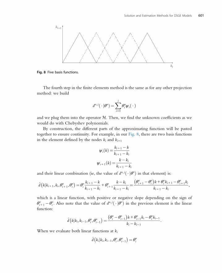
The fourth step in the finite elements method is the same as for any other projection

method: we build

dn, j � jθnð Þ¼Xji¼0

θni ψ i �ð Þ

and we plug them into the operator H. Then, we find the unknown coefficients as we

would do with Chebyshev polynomials.

By construction, the different parts of the approximating function will be pasted

together to ensure continuity. For example, in our Fig. 8, there are two basis functions

in the element defined by the nodes ki and ki+1

ψ i kð Þ¼ ki+1�k

ki+1�ki

ψ i+1 kð Þ¼ k�ki

ki+1�ki

and their linear combination (ie, the value of dn, j � jθnð Þ in that element) is:

d kjki+1,ki,θni+1,θ

ni

� �¼ θniki+1�k

ki+1�ki+ θni+1

k�ki

ki+1�ki¼ θni+1�θni� �

k+ θni ki+1�θni+1ki

ki+1�ki,

which is a linear function, with positive or negative slope depending on the sign of

θni+1�θni . Also note that the value of dn, j � jθnð Þ in the previous element is the linear

function:

d kjki,ki�1,θni ,θ

ni�1

� �¼ θni �θni�1

� �k+ θni�1ki�θni ki�1

ki�ki�1

:

When we evaluate both linear functions at ki

d kijki,ki�1,θni ,θ

ni�1

� �¼ θni

kt+1

kt

Fig. 8 Five basis functions.


and

d kijki+1,ki,θni+1,θ

ni

� �¼ θni

that is, both functions have the same value equal to the coefficient θni , which ensures con-tinuity (although, with only tent functions, we cannot deliver differentiability).

The previous derivation also shows why finite elements are a smart strategy. Imagine

that our metric ρ is such that we want to make the residual function equal to zero in the

nodes of the elements (below we will present a metric like this one). With our tent func-

tions, this amounts to picking, at each ki, the coefficient θni such that the approximating

and exact function coincide:

dn, j � jθnð Þ¼ dn �ð Þ:This implies that the value of dn outside ki are irrelevant for our choice of θ

ni . An exam-

ple of such piecewise linear approximation to a decision rule for the level of debt

tomorrow, bt+1, given capital today, kt, in a model of financial frictions, is drawn in

Fig. 9. The discontinuous line is the approximated decision rule and the continuous line

the exact one. The tent functions are multiplied by the coefficients to make the approx-

imation and the exact solution equal at the node points. We can appreciate an already

high level of accuracy. As the elements become smaller and smaller, the approximation

will become even more accurate (ie, smooth functions are locally linear).

This is a stark example of a more general point: the large system of nonlinear equations

that we will need to solve in a finite element method will be sparse, a property that can be

suitably exploited by modern nonlinear solvers.

Remark 22 (Finite elements method refinements) An advantage of the finite elements

method is that we can refine the solution that we obtain as much as we desire (with only

the constraints of computational time and memory). The literature distinguishes among

bt+1

kt

Fig. 9 Finite element approximation.


three different refinements. First, we have the h-refinement. This scheme subdivides each

element into smaller elements to improve resolution uniformly over the domain. That is,

once we have obtained a first solution, we check whether this solution achieves the

desired level of accuracy. If it does not, we go back to our partition, and we subdivide

the elements. We can iterate in this procedure as often as we need. Second, we have r-

refinement: This scheme subdivides each element only in those regions where there are

high nonlinearities. Third, we have the p-refinement: This scheme increases the order

of the approximation in each element, that is, it adds more basis functions (for example,

several Chebyshev polynomials). If the order of the expansion is high enough, we gen-

erate a hybrid of finite and spectral methods known as spectral elements. This approach

has gained much popularity in the natural sciences and engineering. See, for example,

Solın et al. (2004).

Sometimes, h-refinements and p-refinements are mixed in what is known as the hp-finite

element method, which delivers exponential convergence to the exact solution.

Although difficult to code and computationally expensive, an hp-finite element method

is, perhaps, the most powerful solution technique available for DSGE models, as it can

tackle even the most challenging problems.y

The three refinements can be automatically implemented: we can code the finite ele-

ment algorithm to identify the regions ofΩwhere, according to some goal of interest (for

example, how tightly a Euler equation is satisfied), we refine the approximation without

further input from the researcher. See Demkowicz (2007).

5.5 Objective FunctionsOur second choice is to select a metric function ρ to determine how we “project.” The

most common answer to this question is given by a weighted residual: we select θ to get theresidual close to 0 in the weighted integral sense. Since we did not impose much struc-

ture on the operatorH and therefore, on the residual function R � jθð Þ, we will deal withthe simplest case where R � jθð Þ is unidimensional. More general cases can be dealt with

at the cost of heavier notation. Given some weight functions ϕi :Ω!, we define themetric:

ρ R � jθð Þ,0ð Þ¼ 0 ifRΩϕi xð ÞR � jθð Þdx¼ 0, i¼ 1, ::, j+1

1 otherwise

�

y An additional, new refinement is the extended finite element method (x-fem), which adds to the basis

discontinuous functions that can help in capturing irregularities in the solution. We are not aware of

applications of the x-fem in economics.


Hence, the problem is to choose the θ that solves the system of integral equations:ZΩϕi xð ÞR � jθð Þdx¼ 0, i¼ 1, ::, j+1: (39)

Note that, for the system to have a solution, we need j + 1 weight functions. Thanks to

the combination of approximating the function d by basis functions ψ i and the definition

of weight functions ϕi, we have transformed a rather intractable functional equation

problem into a standard nonlinear equations system. The solution of this system can

be found using standard methods, such as a Newton algorithm for small problems or a

Levenberg–Marquardt method for bigger ones.

However, the system (39) may have no solution or it may have multiple ones. We

know very little about the theoretical properties of projection methods in economic

applications. The literature in applied mathematics was developed for the natural sciences

and engineering and many of the technical conditions required for existence and conver-

gence theorems to work do not easily travel across disciplines. In fact, some care must be

put into ensuring that the solution of the system (39) satisfies the transversality conditions

of the DSGEmodel (ie, we are picking the stable manifold). This can usually be achieved

with the right choice of an initial guess θ0 or by adding boundary conditions to the solver.As was the case with the bases, we will have plenty of choices for our weight func-

tions. Instead of reviewing all possible alternatives, we will focus on the most popular

ones in economics.

5.5.1 Weight Function I: Least SquaresLeast squares use as weight functions the derivatives of the residual function:

ϕi xð Þ¼ @R xjθð Þ@θi�1

for all i 2 1,.., j + 1. This choice is motivated by the variational problem:

minθ

ZΩR2 � jθð Þdx

with first-order condition:ZΩ

@R xjθð Þ@θi�1

R � jθð Þdx¼ 0, i¼ 1, ::, j+1:

This variational problem is mathematically equivalent to a standard regression problem

in econometrics.

While least squares are intuitive and there are algorithms that exploit some of their

structure to increase speed and decrease memory requirements, they require the compu-

tation of the derivative of the residual, which can be costly. Also, least squares problems

are often ill-conditioned and complicated to solve numerically.


5.5.2 Weight Function II: SubdomainThe subdomain approach divides the domainΩ into 1,.., j + 1 subdomainsΩi and define

the j + 1 step functions:

ϕi xð Þ¼ 1 if x2Ωi

0 otherwise

�

This choice is equivalent to solving the system:ZΩi

R � jθð Þdx¼ 0, i¼ 1, ::, j+1:

The researcher has plenty of flexibility to pick her subdomains as to satisfy her criteria of

interest.

5.5.3 Weight Function III: CollocationThis method is also known as pseudospectral or the method of selected points. It defines

the weight function as:

ϕi xð Þ¼ δ x�xið Þwhere δ is the Dirac delta function and xi are the j + 1 collocation points selected by the

researcher.

This method implies that the residual function is zero at the n collocation points. Thus,

instead of having to compute complicated integrals, we only need to solve the system:

R xijθð Þ¼ 0, i¼ 1, ::, j+1:

This is attractive when the operator H generates large nonlinearities.

A systematic way to pick collocation points is to use the zeros of the j+1ð Þ-th-orderChebyshev polynomial in each dimension of the state variable (or the corresponding

polynomials, if we are using different approximation orders along each dimension). This

approach is known as orthogonal collocation. The Chebyshev interpolation theorem tells

us that, with this choice of collocation points, we can achieveLp convergence and some-

times even uniform convergence to the unknown function d. Another possibility is to

pick, as collocation points, the extrema of the j-th-order Chebyshev polynomial in each

dimension. Experience shows a surprisingly good performance of orthogonal collocation

methods and it is one of our recommended approaches.

5.5.4 Weight Function IV: Galerkin or Rayleigh–RitzThe last weight function we consider is the Galerkin (also called Rayleigh–Ritz when it

satisfies some additional properties of less importance for economists). This approach

takes as the weight function the basis functions used in the approximation:

ϕi xð Þ¼ψ i�1 xð Þ:


Then we have: ZΩψ i xð ÞR � jθð Þdx¼ 0, i¼ 1, ::, j+1:

The interpretation is that the residual has to be orthogonal to each of the basis functions.

The Galerkin approach is highly accurate and robust, but difficult to code. If the basis

functions are complete over J1 (they are indeed a basis of the space), then the Galerkin

solution will converge pointwise to the true solution as n goes to infinity:

limj!∞

dj � jθð Þ¼ d �ð ÞAlso, practical experience suggests that a Galerkin approximation of order j is as accurate

as a pseudospectral j + 1 or j + 2 expansion.

In the next two remarks, we provide some hints for a faster and more robust solution

of the system of nonlinear equations:ZΩϕi xð ÞR � jθð Þdx¼ 0, i¼ 1, ::, j+1, (40)

a task that can be difficult if the number of coefficients is large and the researcher does not

have a good initial guess θ0 for the solver.

Remark 23 (Transformations of the problem) A bottleneck for the solution of (39) can be

the presence of strong nonlinearities. Fortunately, it is often the case that simple changes

in the problem can reduce these nonlinearities. For example, Judd (1992) proposes that if

we have an Euler equation:

1

ct¼ βt

1

ct+1

Rt+1

� �

where Rt+1 is the gross return rate of capital, we can take its inverse:

βct ¼ t

1

ct+1

Rt+1

� � ��1

,

which now is linear on the left-hand side and much closer to linear on the right-hand

side. Thus, instead of computing the residual for some state variable xt

R � jθð Þ¼ 1

c xtjθð Þ�βt

1

c xtjθð ÞRt+1 xtjθð Þ� �

,

we compute:

R� � jθð Þ¼ βc xtjθð Þ� t

1

c xtjθð ÞRt+1 xtjθð Þ� � ��1

:

Similar algebraic manipulations are possible in many DSGE models.


Remark 24 (Multistep schemes) The system (39) can involve a large number of coeffi-

cients. A natural strategy is to solve first a smaller system and to use that solution as an

input for a larger system. This strategy, called a multistep scheme, often delivers excellent

results, in particular when dealing with orthogonal bases such as Chebyshev polynomials.

More concretely, instead of solving the system for an approximation with j + 1 basis

functions, we can start by solving the system with only j0 +1≪ j+1 basis functions and

use the solution to this first problem as a guess for the more complicated problem. For

example, if we are searching for a solution with 10 Chebyshev polynomials andm dimen-

sions, we first find the approximation with only 3 Chebyshev polynomials. Therefore,

instead of solving a system of 10 � m equations, we solve a system of 3 � m. Once

we have the solution θ3, we build the initial guess for the problem with 10 Chebyshev

polynomials as:

θ0¼ θ3,01�m,…,01�m

� �,

that is, we use θ3 for the first coefficients and zero for the additional new coefficients.

Since the additional polynomials are orthogonal to the previous ones, the final values

of the coefficients associated with the three first polynomials will change little with

the addition of 7more polynomials: the initial guess θ3 is, thus, most splendid. Also, given

the fast convergence of Chebyshev polynomials, the coefficients associated with higher-

order polynomials will be close to zero. Therefore, our initial guess for those coefficients

is also informative.

The researcher can use as many steps as she needs. By judiciously coding the projec-

tion solver, the researcher can write the program as depending on an abstract number of

Chebyshev polynomials. Then, she can call the solver inside a loop and iteratively

increase the level of approximation from j0 to j as slow or as fast as required.

5.6 A Worked-Out ExampleWe present now a worked-out example of how to implement a projection method in a

DSGE model. In particular, we will use Chebyshev polynomials and orthogonal collo-

cation to solve the stochastic neoclassical growth model with endogenous labor supply.

In this economy, there is a representative household, whose preferences over

consumption, ct, and leisure, 1 � lt, are representable by the utility function:

0

X∞t¼1

βt�1 cτt 1� ltð Þ1�τ� �1�η

1�η

where β2 0,1ð Þ is the discount factor, η controls the elasticity of intertemporal substitu-

tion and risk aversion, τ controls labor supply, and 0 is the conditional expectation

operator.


There is one good in the economy, produced according to the aggregate production

function:

yt ¼ ezt kαt l1�αt

where kt is the aggregate capital stock, lt is aggregate labor, and zt is a stochastic process

for technology:

zt ¼ ρzt�1 + Et

with ρj j< 1 and Et � N(0, σ2). Capital evolves according to:

kt+1¼ð1�δÞkt + it

and the economy must satisfy the resource constraint yt ¼ ct + it.

Since both welfare theorems hold in this economy, we solve directly for the social

planner’s problem:

V kt,ztð Þ¼ maxct, lt

cτt 1� ltð Þ1�τ� �1�η

1�η+ βtV kt+1,zt+1ð Þ

s:t: kt+1¼ ezt kαt l1�αt + ð1�δÞkt� ct

zt ¼ ρzt�1 + Et

given some initial conditions k0 and z0. Tackling the social planner’s problem is only

done for convenience, and we could also solve for the competitive equilibrium. In fact,

one key advantage of projection methods is that they easily handle non-Pareto efficient

economies.

We calibrate the model with standard parameter values to match US quarterly data

(see Table 2). The only exception is η, for which we pick a value of 5, in the higher rangeof empirical estimates. Such high-risk aversion induces, through precautionary behavior,

more curvature in the decision rules. This curvature would present a more challenging

test bed for the projection method.

We discretize zt into a 5-point Markov chain z1,…,z5f g using Tauchen’s procedureand covering3 unconditional standard deviations of zt (this is the sameMarkov chain as

Table 2 CalibrationParameter Value

β 0.991

η 5.000

τ 0.357

α 0.300

δ .0196

ρ 0.950

σ 0.007


the example in Remark 21, see (36) and (37) for the concrete values of the discretization).

We will use pmn to denote the generic entry of the transition matrix Pz,z0 generated by

Tauchen’s procedure for zm today moving to zn next period.

Then, we approximate the value function V j ktð Þ and the decision rule for labor,

lj ktð Þ, for j ¼ 1,…,5 using 11 Chebyshev polynomials as:

V j ktjθV , j� �¼X10

i¼0

θV , ji Ti ktð Þ (41)

lj ktjθl, j� �¼X10

i¼0

θl,ki Ti ktð Þ (42)

Once we have the decision rule for labor, we can find output:

yj ktð Þ¼ ezt kαt lj ktjθl, j� �� 1�α

,

With output, from the first-order condition that relates the marginal utility consumption

and the marginal productivity of labor, we can find consumption:

cj ktð Þ¼ τ

1� τð1�αÞezt kαt lj ktjθl, j

� �� α1� lj ktjθl, j

� �� (43)

and, from the resource constraint, capital next period:

kj ktð Þ¼ eztkαt lj ktjθl, j� �� 1�α

+ ð1�δÞkt� cj ktð Þ (44)

Our notations yj ktð Þ, cj ktð Þ, and kj ktð Þ emphasize the exact dependence of these three

variables on capital and the productivity level: once we have approximated lj ktjθl, j� �

,

simple algebra with the equilibrium conditions allows us to avoid further approximation.

We decided to approximate the value function and the decision rule for labor and use

them to derive the other variables of interest to illustrate how flexible projection methods

are. We could, as well, have decided to approximate the decision rules for consumption

and capital and find labor and the value function using the equilibrium conditions. The

researcher should pick the approximating functions that are more convenient, either for

algebraic reasons or her particular goals.

To solve for the unknown coefficients θV and θl, we plug the functions (41), (42),

(43), and (44) into the Bellman equation to get:

X10i¼0

θV , ji Ti ktð Þ¼

cj ktð Þð Þθ 1�P10i¼0θ

liTi ktð Þ� �1�θ

� �1�τ

1� τ+ βX5m¼1

pjmX10i¼0

θV , ji Ti k

j ktð Þ� �(45)

where, since we are already using the optimal decision rules, we can drop the max oper-

ator. Also, we have substituted the expectation by the sum operator and the transition


probabilities pjm. We plug the same functions (41), (42), (43), and (44) into the Euler

equation to get:

cθt 1�P10i¼0θ

l,ki Ti ktð Þ� �1�θ

� �1�τ

ct¼ βt

X5m¼1

pjmX10i¼0

θV , ji Ti k

j ktð Þ� �0, (46)

where Ti kj ktð Þð Þ0 is the derivative of the Chebyshev polynomial with respect to its

argument.

The residual equation groups Eqs. (45) and (46):

R kt, zj��θ� �¼

P10i¼0θ

V , ji Ti ktð Þ�

cj ktð Þð Þθ 1�P10i¼0θ

liTi ktð Þ� �1�θ

� �1�τ

1� τ

�βP5

m¼1 pjmP10

i¼0θV , ji Ti k

j ktð Þ� �cθt 1�P10

i¼0θl,ki Ti ktð Þ� �1�θ

� �1�τ

ct�βt

X5

m¼1pjmX10

i¼0θV , ji Ti k

j ktð Þ� �0

8>>>>>>>>><>>>>>>>>>:

where θ stacks θV, j and θl,k. Given that we use 11 Chebyshev polynomials for the value

function and another 11 for the decision rule for labor for each of the 5 levels of zj, θ has110 elements (110 ¼ 11 � 2 � 5). If we evaluate the residual function at each of the

11 zeros of the Chebyshev of order 11 for capital and the 5 levels of zj, we will have

the 110 equations required to solve for those 110 coefficients. ANewton solver can easily

deal with this system (although, as explained in Remark 24, using a multistep approach

simplifies the computation: we used 3 Chebyshev polynomials in the first step and

11 Chebyshev polynomials in the second one).

We plot the main components of the solution in Fig. 10. The top left panel draws the

value function, with one line for each of the five values of productivity and capital on the

x-axis. As predicted by theory, the value function is increasing and concave in both

state variables, kt and zt. We follow the same convention for the decision rules for

consumption (top right panel), labor supply (bottom left panel), and capital next period,

kt+1 (bottom right panel). The most noticeable pattern is the near linearity of the capital

decision rule. Once the researcher has found the value function and all the decision rules,

she can easily simulate the model, compute impulse response functions, and evaluate

welfare.

The accuracy of the solution is impressive, with Euler equation errors below -13

in the log10 scale. Section 7 discusses how to interpret these errors. Suffice it to say

here that, for practical purposes, the solution plotted in Fig. 10 can be used instead

of the exact solution of the stochastic neoclassical growth model with a discrete produc-

tivity level.


5.7 Smolyak's AlgorithmAn alternative to complete polynomials that can handle the curse of dimensionality better

than other methods is Smolyak’s algorithm. See Smolyak (1963), Delvos (1982),

Barthelmann et al. (2000), and, especially, Bungartz and Griebel (2004) for a summary

of the literature. Kr€uger and Kubler (2004) and Malin et al. (2011) introduced the algo-

rithm in economics as a solution method for DSGE models. Subsequently, Smolyak’s

algorithm has been applied by many researchers. For example, Fernandez-Villaverde

et al. (2015a) rely on Smolyak’s algorithm to solve a New Keynesian model with a

ZLB (a model with 5 state variables), Fernandez-Villaverde and Levintal (2016) exploit

it to solve a NewKeynesian model with big disasters risk (a model with 12 state variables),

andGordon (2011) uses it to solve a model with heterogeneous agents.Malin et al. (2011)

can accurately compute a model with 20 continuous state variables and a considerable

deal of curvature in the production and utility functions. In the next pages, we closely

follow the explanations in Kr€uger and Kubler (2004) and Malin et al. (2011) and invite

the reader to check those papers for further details.z

Fig. 10 Solution, stochastic neoclassical growth model.

z There is also a promising line of research based on the use of ergodic sets to solve highly dimensional models

(Judd et al., 2011b; Maliar et al., 2011; and Maliar and Maliar, 2015). Maliar and Maliar (2014) cover the

material better than we could.


As before, we want to approximate a function (decision rule, value function, expec-

tation, etc.) on n state variables, d : ½�1,1�n ! (the generalization to the case

d : ½�1,1�n !m is straightforward, but tedious). The idea of Smolyak’s algorithm is

to find a grid of points ðq,nÞ 2 ½�1,1�n where q > n and an approximating function

dðxjθ, q, nÞ : ½�1,1�n! indexed by some coefficients θ such that, at the points

xi 2ðq,nÞ, the unknown function d �ð Þ and d(�jθ, q, n) are equal:d xið Þ¼ dðxijθ, q, nÞ

and, at the points xi 62 ðq,nÞ, d(�jθ, q, n) is close to the unknown function d �ð Þ. In otherwords, at the points xi 2 ðq, nÞ, the operator H �ð Þ would be exactly satisfied and, at

other points, the residual function would be close to zero. The integer q indexes the size

of the grid and, with it, the precision of the approximation.

The challenge is to judiciously select grid pointsðq,nÞ in such a way that the number

of coefficients θ does not explode with n. Smolyak’s algorithm is (almost) optimal for that

task within the set of polynomial approximations (Barthelmann et al., 2000). Also, the

method is universal, that is, almost optimal for many different function spaces.

5.7.1 Implementing Smolyak's AlgorithmOur search of a grid of points ðq,nÞ and a function d(xjθ,q,n) will proceed in several

steps.

5.7.1.1 First Step: Transform the Domain of the State VariablesFor any state variable x

�l, l ¼ 1,…,n that has a domain a,b½ �, we use a linear translation

from a,b½ � into �1,1½ � :

xl ¼ 2x�l� a

b� a�1:

5.7.1.2 Second Step: Setting the Order of the PolynomialWe define m1 ¼ 1 and mi ¼ 2i�1 + 1, i ¼ 2,…, where mi � 1 will be the order of the

polynomial that we will use to approximate d �ð Þ.

5.7.1.3 Third Step: Building the Gauss–Lobotto NodesWe build the sets:

Gi ¼fζi1,…,ζimig� ½�1,1�

that contain the Gauss–Lobotto nodes (also known as the Clenshaw–Curtis points), that

is, the extrema of the Chebyshev polynomials:


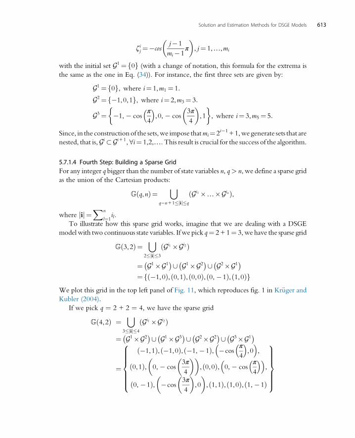
ζij ¼�cosj�1

mi�1π

�, j¼ 1,…,mi

with the initial set G1¼f0g (with a change of notation, this formula for the extrema is

the same as the one in Eq. (34)). For instance, the first three sets are given by:

G1¼f0g, where i¼ 1,m1¼ 1:

G2¼f�1,0,1g, where i¼ 2,m3¼ 3:

G3¼ �1, � cosπ

4

� �,0, � cos

3π

4

�,1

� �, where i¼ 3,m5¼ 5:

Since, in the constructionof the sets,we impose thatmi¼2i�1+1,wegenerate sets that are

nested, that is,Gi�Gi+1, 8i¼ 1,2,…. This result is crucial for the success of the algorithm.

5.7.1.4 Fourth Step: Building a Sparse GridFor any integer q bigger than the number of state variables n, q> n, we define a sparse grid

as the union of the Cartesian products:

ðq,nÞ¼[

q�n+1�jij�q

ðGi1 �…�GinÞ,

where ij j ¼Xn

l¼1il.

To illustrate how this sparse grid works, imagine that we are dealing with a DSGE

model with two continuous state variables. If we pick q¼ 2+ 1¼ 3, we have the sparse grid

3,2ð Þ¼[

2�jij�3

ðGi1 �Gi2Þ

¼ G1�G1� �[ G1�G2

� �[ G2�G1� �

¼ �1,0ð Þ, 0,1ð Þ, 0,0ð Þ, 0,�1ð Þ, 1,0ð Þf gWe plot this grid in the top left panel of Fig. 11, which reproduces fig. 1 in Kr€uger andKubler (2004).

If we pick q ¼ 2 + 2 ¼ 4, we have the sparse grid

ð4,2Þ ¼[

3�jij�4

ðGi1 �Gi2Þ

¼ G1�G2� �[ G1�G3

� �[ G2�G2� �[ G3�G1

� �

¼

�1,1ð Þ, �1,0ð Þ, �1, �1ð Þ, �cosπ

4

� �,0

� �,

0,1ð Þ, 0, � cos3π

4

� �, 0,0ð Þ, 0, � cos

π

4

� �� ,

0, �1ð Þ, �cos3π

4

�,0

�, 1,1ð Þ, 1,0ð Þ, 1, �1ð Þ

8>>>>><>>>>>:

9>>>>>=>>>>>;


We plot this grid in the top right panel of Fig. 11. Note that the sparse grids have a

hierarchical structure, where 3,2ð Þ 2 4,2ð Þ or, more generally, q,nð Þ 2 q+1,nð Þ.Following the same strategy, we can build ð5,2Þ, plotted in the bottom left panel

of Fig. 11, and ð6,2Þ, plotted in the bottom right panel of Fig. 11 (in the interest of

concision, we skip the explicit enumeration of the points of these two additional grids).

In Fig. 12, we plot a grid for a problem with 3 state variables, ð5,3Þ.The sparse grid has two important properties. First, the grid points cluster around

the corners of the domain of the Chebyshev polynomials and the central cross. Second,

the number of points in a sparse grid when q¼ n + 2 is given by 1 + 4n + 2n(n� 1). The

cardinality of this grid grows polynomially on n2. Similar formulae hold for other q > n.

For example, the cardinality of the grid grows polynomially on n3 when q¼ n+ 3. In fact,

the computational burden of the method notably increases as we keep n fixed and a rise q.

Fortunately, experience suggests that q ¼ n + 2 and q ¼ n + 3 are usually enough to

deliver the desired accuracy in DSGE models.

The nestedness of the sets of the Gauss–Lobotto nodes plays a central role in

controlling the cardinality of ðq,nÞ. In comparison, the number of points in a rect-

angular grid is 5n, an integer that grows exponentially on n. If n ¼ 2, this would

correspond, in the top right panel of Fig. 11, to having all possible tensors of

–1 –0.5 0 0.5 1–1

–0.5

0

0.5

1

–1 –0.5 0 0.5 1–1

–0.5

0

0.5

1

–1 –0.5 0 0.5 1–1

–0.5

0

0.5

1

–1 –0.5 0 0.5 1–1

–0.5

0

0.5

1

Fig. 11 Four sparse grids


�1, � cosπ

4

� �,0, � cos

3π

4

�,1

� �and �1, � cos

π

4

� �,0, � cos

3π

4

�,1

� �cover-

ing the whole of the [�1,1]2 square. Instead of keeping these 25 points, Smolyak’s

algorithm eliminates 12 of them and only keeps 13. To illustrate how dramatic is

the difference between polynomial and exponential growth, Table 3 shows the car-

dinality of both grids as we move from 2 state variables to 12.

5.7.1.5 Fifth Step: Building Tensor ProductsWe use the Chebyshev polynomials ψ i xið Þ¼Ti�1 xið Þ to build the tensor-product

multivariate polynomial:

–0.50

0.51

–1–1

–0.5

0

0.5

1–1

–0.5

0

0.5

1

Fig. 12 A sparse grid, 3 state variables.

Table 3 Size of the grid for q ¼ n + 2n ðq,nÞ 5n

2 13 25

3 25 125

4 41 625

5 61 3125

12 313 244,140,625


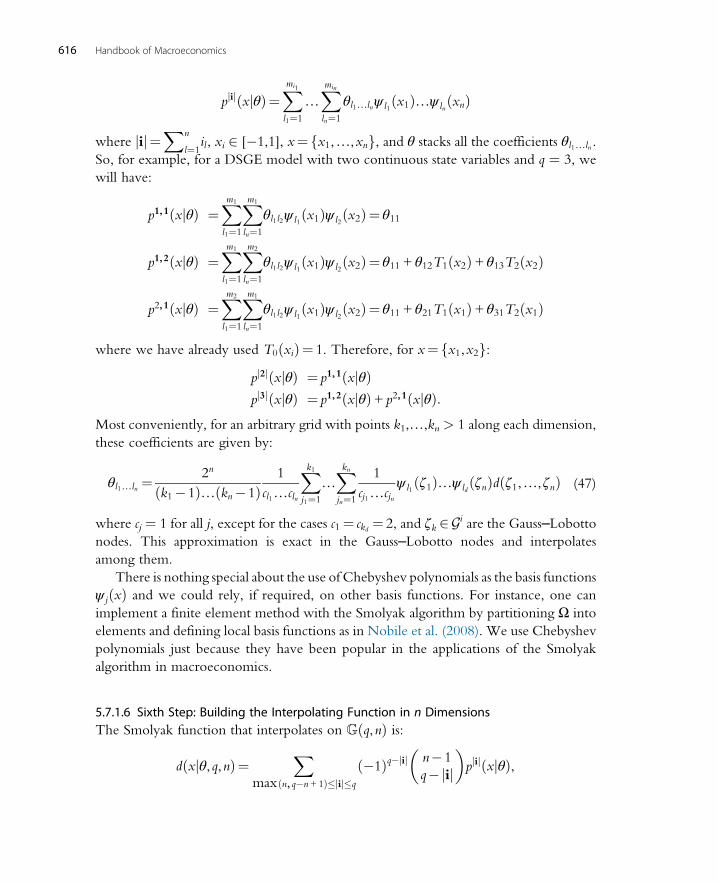
p ij jðxjθÞ¼Xmi1

l1¼1

…

Xmin

ln¼1

θl1…lnψ l1x1ð Þ…ψ ln

xnð Þ

where ij j ¼Xn

l¼1il, xi 2 [�1,1], x¼ x1,…,xnf g, and θ stacks all the coefficients θl1…ln .

So, for example, for a DSGE model with two continuous state variables and q ¼ 3, we

will have:

p1,1ðxjθÞ ¼Xm1

l1¼1

Xm1

ln¼1

θl1l2ψ l1x1ð Þψ l2

x2ð Þ¼ θ11

p1,2ðxjθÞ ¼Xm1

l1¼1

Xm2

ln¼1


x2ð Þ¼ θ11 + θ12T1 x2ð Þ+ θ13T2 x2ð Þ

p2,1ðxjθÞ ¼Xm2

l1¼1

Xm1

ln¼1


x2ð Þ¼ θ11 + θ21T1 x1ð Þ+ θ31T2 x1ð Þ

where we have already used T0 xið Þ¼ 1. Therefore, for x¼ x1,x2f g:p 2j j xjθð Þ ¼ p1,1ðxjθÞp 3j j xjθð Þ ¼ p1,2ðxjθÞ+ p2,1ðxjθÞ:

Most conveniently, for an arbitrary grid with points k1,…,kn > 1 along each dimension,

these coefficients are given by:

θl1…ln ¼2n

k1�1ð Þ… kn�1ð Þ1

cl1…cln

Xk1j1¼1

…

Xknjn¼1

1

cj1…cjnψ l1

ζ1ð Þ…ψ ldζnð Þd ζ1,…,ζnð Þ (47)

where cj ¼ 1 for all j, except for the cases c1¼ ckd ¼ 2, and ζk 2Gi are the Gauss–Lobotto

nodes. This approximation is exact in the Gauss–Lobotto nodes and interpolates

among them.

There is nothing special about the use of Chebyshev polynomials as the basis functions

ψ j xð Þ and we could rely, if required, on other basis functions. For instance, one can

implement a finite element method with the Smolyak algorithm by partitioning Ω into

elements and defining local basis functions as in Nobile et al. (2008). We use Chebyshev

polynomials just because they have been popular in the applications of the Smolyak

algorithm in macroeconomics.

5.7.1.6 Sixth Step: Building the Interpolating Function in n DimensionsThe Smolyak function that interpolates on ðq,nÞ is:

dðxjθ,q,nÞ¼X

max n,q�n+1ð Þ�jij�q

ð�1Þq�jij n�1

q�jij �

p ij jðxjθÞ,


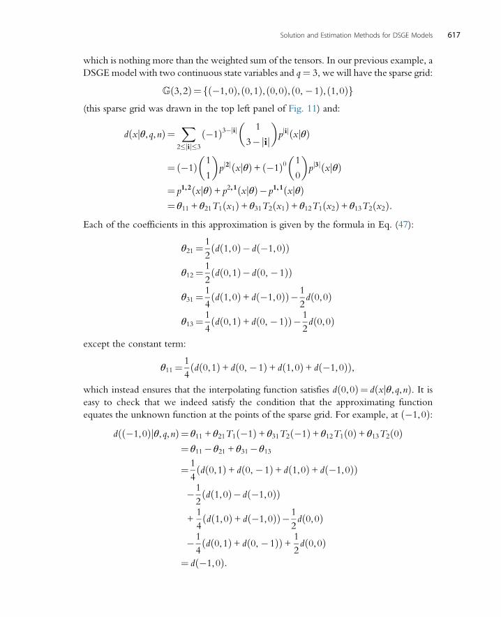
which is nothing more than the weighted sum of the tensors. In our previous example, a

DSGEmodel with two continuous state variables and q¼ 3, we will have the sparse grid:

ð3,2Þ¼ �1,0ð Þ, 0,1ð Þ, 0,0ð Þ, 0,�1ð Þ, 1,0ð Þf g(this sparse grid was drawn in the top left panel of Fig. 11) and:

dðxjθ,q,nÞ¼X

2�jij�3

ð�1Þ3�jij 1

3�jij

�p ij jðxjθÞ

¼ ð�1Þ 1

1

�p 2j jðxjθÞ+ ð�1Þ0 1

0

�p 3j jðxjθÞ

¼ p1,2ðxjθÞ+ p2,1ðxjθÞ�p1,1ðxjθÞ¼ θ11 + θ21T1 x1ð Þ+ θ31T2 x1ð Þ+ θ12T1 x2ð Þ+ θ13T2 x2ð Þ:

Each of the coefficients in this approximation is given by the formula in Eq. (47):

θ21¼ 1

2d 1,0ð Þ� d �1,0ð Þð Þ

θ12¼ 1

2d 0,1ð Þ� d 0, �1ð Þð Þ

θ31¼ 1

4d 1,0ð Þ+ d �1,0ð Þð Þ�1

2d 0,0ð Þ

θ13¼ 1

4d 0,1ð Þ+ d 0, �1ð Þð Þ�1

2d 0,0ð Þ

except the constant term:

θ11¼ 1

4d 0,1ð Þ+ d 0, �1ð Þ+ d 1,0ð Þ+ d �1,0ð Þð Þ,

which instead ensures that the interpolating function satisfies d 0,0ð Þ¼ dðxjθ,q,nÞ. It iseasy to check that we indeed satisfy the condition that the approximating function

equates the unknown function at the points of the sparse grid. For example, at �1,0ð Þ:dð �1,0ð Þjθ,q,nÞ¼ θ11 + θ21T1 �1ð Þ+ θ31T2 �1ð Þ+ θ12T1 0ð Þ+ θ13T2 0ð Þ

¼ θ11�θ21 + θ31�θ13

¼ 1

4d 0,1ð Þ+ d 0, �1ð Þ+ d 1,0ð Þ+ d �1,0ð Þð Þ

�1

2d 1,0ð Þ�d �1,0ð Þð Þ

+1

4d 1,0ð Þ+ d �1,0ð Þð Þ�1

2d 0,0ð Þ

�1

4d 0,1ð Þ+ d 0, �1ð Þð Þ+ 1

2d 0,0ð Þ

¼ d �1,0ð Þ:


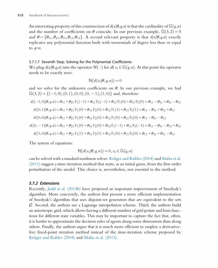
An interesting property of this construction of d(xjθ,q,n) is that the cardinality ofðq,nÞand the number of coefficients on θ coincide. In our previous example, ð3,2Þ ¼ 5

and θ¼ θ11,θ21,θ31,θ12,θ13f g. A second relevant property is that d(xjθ,q,n) exactlyreplicates any polynomial function built with monomials of degree less than or equal

to q–n.

5.7.1.7 Seventh Step: Solving for the Polynomial CoefficientsWe plug d(xjθ,q,n) into the operatorH �ð Þ for all xi 2ðq,nÞ. At this point the operatorneeds to be exactly zero:

H dðxijθ,q,nÞð Þ¼ 0

and we solve for the unknown coefficients on θ. In our previous example, we had

ð3,2Þ¼ �1,0ð Þ, 0,1ð Þ, 0,0ð Þ, 0, �1ð Þ, 1,0ð Þf g and, therefore:

dð �1,0ð Þjθ,q,nÞ¼ θ11 + θ21T1 �1ð Þ+ θ31T2 �1ð Þ+ θ12T1 0ð Þ+ θ13T2 0ð Þ¼ θ11�θ21 + θ31�θ13

dð 0,1ð Þjθ,q,nÞ¼ θ11 + θ21T1 0ð Þ+ θ31T2 0ð Þ+ θ12T1 1ð Þ+ θ13T2 1ð Þ¼ θ11�θ31 + θ12 + θ13

dð 0,0ð Þjθ,q,nÞ¼ θ11 + θ21T1 0ð Þ+ θ31T2 0ð Þ+ θ12T1 0ð Þ+ θ13T2 0ð Þ¼ θ11�θ31�θ13

dð 0, �1ð Þjθ,q,nÞ¼ θ11 + θ21T1 0ð Þ+ θ31T2 0ð Þ+ θ12T1 �1ð Þ+ θ13T2 �1ð Þ¼ θ11�θ31�θ12 + θ13

dð 1,0ð Þjθ,q,nÞ¼ θ11 + θ21T1 1ð Þ+ θ31T2 1ð Þ+ θ12T1 0ð Þ+ θ13T2 0ð Þ¼ θ11 + θ21 + θ31�θ13

The system of equations:

H dðxijθ,q,nÞð Þ¼ 0, xi 2ðq,nÞcan be solved with a standard nonlinear solver. Kr€uger and Kubler (2004) andMalin et al.

(2011) suggest a time-iteration method that starts, as an initial guess, from the first-order

perturbation of the model. This choice is, nevertheless, not essential to the method.

5.7.2 ExtensionsRecently, Judd et al. (2014b) have proposed an important improvement of Smolyak’s

algorithm. More concretely, the authors first present a more efficient implementation

of Smolyak’s algorithm that uses disjoint-set generators that are equivalent to the sets

Gi. Second, the authors use a Lagrange interpolation scheme. Third, the authors build

an anisotropic grid, which allows having a different number of grid points and basis func-

tions for different state variables. This may be important to capture the fact that, often,

it is harder to approximate the decision rules of agents along some dimensions than along

others. Finally, the authors argue that it is much more efficient to employ a derivative-

free fixed-point iteration method instead of the time-iteration scheme proposed by

Kr€uger and Kubler (2004) and Malin et al. (2011).


In comparison, Brumm and Scheidegger (2015) keep a time-iteration procedure,

but they embed on it an adaptive sparse grid. This grid is refined locally in an automatic

fashion, which allows the capture of steep gradients and some nondifferentiabilities.

The authors provide a fully hybrid parallel implementation of the method, which takes

advantage of the fast improvements in massively parallel processing.

6. COMPARISON OF PERTURBATION AND PROJECTION METHODS

After our description of perturbation and projection methods, we can offer some brief

comments on their relative strengths and weaknesses.

Perturbation methods have one great advantage: their computational efficiency. We

can compute, using a standard laptop computer, a third-order approximation to DSGE

models with dozens of state variables in a few seconds. Perturbation methods have one

great disadvantage: they only provide a local solution. The Taylor series expansion is

accurate around the point at which we perform the perturbation and deteriorates as

we move away from that point. Although perturbation methods often yield good global

results (see Aruoba et al., 2006; Caldara et al., 2012; and Swanson et al., 2006), such

performance needs to be assessed in each concrete application and even a wide range

of accuracy may not be sufficient for some quantitative experiments. Furthermore,

perturbation relies on differentiability conditions that are often violated by models of

interest, such as those that present kinks or occasionally binding constraints.aa

Projection methods are nearly the mirror image of perturbation. Projection methods

have one great advantage: Chebyshev and finite elements produce solutions that are of

high accuracy over the whole range of state variable values. See, again, Aruoba et al.

(2006) and Caldara et al. (2012). And projection methods can attack even the most com-

plex problems with occasionally binding constraints, irregular shapes, and local behavior.

But power and flexibility come at a cost: computational effort. Projection methods are

harder to code, take longer to run, and suffer, as we have repeatedly pointed out, from an

acute curse of dimensionality.ab

Thus, which method to use in real life? The answer, not unsurprisingly, is

“it depends.” Solution methods for DSGE models provide a menu of options. If we

are dealing, for example, with a standard middle-sized New Keynesian model with

aa Researchers have proposed getting around these problems with different devices, such as the use of penalty

functions. See, for example, Preston and Roca (2007). In fact, the recent experience of several central

banks pushing their target interest rates below zero suggests that many constraints such as the ZLB

may be closer to such a penalty function than to a traditional kink.ab The real bottleneck for most research projects involving DSGE models is coding time, not running time.

Moving from a few seconds of running time with perturbation to a few minutes of running time with

projection is a minuscule fraction of the cost of coding a finite elements method in comparison with

the cost of employing Dynare to find a perturbation.


25 state variables, perturbation methods are likely to be the best option. The New

Keynesian model is sufficiently well behaved that a local approximation would be good

enough for most purposes. A first-order approximation will deliver accurate estimates of

the business cycle statistics such as variances and covariances, and a second- or third-order

approximation is likely to generate good welfare estimates (although one should always

be careful when performing welfare evaluations). If we are dealing, in contrast, with a

DSGEmodel with financial constraints, large risk aversion, and only a few state variables,

a projection method is likely to be a superior option. An experienced researcher may

even want to have two different solutions to check one against the other, perhaps of

a simplified version of the model, and decide which one provides her with a superior

compromise between coding time, running time, and accuracy.

Remark 25 (Hybrid methods) The stark comparison between perturbation and projec-

tion methods hints at the possibility of developing hybrid methods that combine the best

of both approaches. Judd (1998, section 15.6), proposes the following hybrid algorithm:

Algorithm 4 (Hybrid algorithm)

1. Use perturbation to build a basis tailored to the DSGE model we need to solve.

2. Apply a Gram-Schmidt process to build an orthogonal basis from the basis obtained

in 1.

3. Employ a projection method with the basis from 2.

While this algorithm is promising (see the example provided by Judd, 1998), we are

unaware of further explorations of this proposal.

More recently, Levintal (2015b) and Fernandez-Villaverde and Levintal (2016)

have proposed the use of Taylor-based approximations that also have the flavor of a

hybrid method. The latter paper shows the high accuracy of this hybrid method in

comparison with pure perturbation and projection methods when computing a DSGE

model with disaster risk and a dozen state variables. Other hybrid proposals include

Maliar et al. (2013).

7. ERROR ANALYSIS

A final step in every numerical solution of a DSGE model is to assess the error created

by the approximation, that is, the difference between the exact and the approximated

solution. This may seem challenging since the exact solution of the model is unknown.

However, the literature has presented different methods to evaluate the errors.ac We will

concentrate on the two most popular procedures to assess error: χ2 �test proposed by

ac Here we follow much of the presentation of Aruoba et al. (2006), where the interested reader can find

more details.


Den Haan and Marcet (1994) and the Euler equation error proposed by Judd (1992).

Throughout this section, we will use the superscript j to index the perturbation order,

the number of basis functions, or another characteristic of the solution method. For

example, cj kt,ztð Þ will be the approximation to the decision rule for consumption

c kt,ztð Þ in a model with state variables kt and zt.

Remark 26 (Theoretical bounds) There are (limited) theoretical results bounding the

approximation errors and their consequences. Santos and Vigo-Aguiar (1998) derive

upper bounds for the error in models computed with value function iteration. Santos

and Rust (2004) extend the exercise for policy function iteration. Santos and Peralta-

Alva (2005) propose regularity conditions under which the error from the simulated

moments of the model converge to zero as the approximated equilibrium function

approaches the exact, but unknown, equilibrium function. Fernandez-Villaverde et al.

(2006) explore similar conditions for likelihood functions and Stachurski and Martin

(2008) perform related work for the computation of densities of ergodic distributions

of variables of interest. Judd et al. (2014a) have argued for the importance of constructing

lower bounds on the size of approximation errors and propose a methodology to do so.

Kogan and Mitra (2014) have studied the information relaxation method of Brown et al.

(2010) to measure the welfare cost of using approximated decision rules. Santos and

Peralta-Alva (2014) review the existing literature. But, despite all this notable work, this

is an area in dire need of further investigation.

Remark 27 (Preliminary assessments) Before performing a formal error analysis,

researchers should undertake several preliminary assessments. First, we need to check that

the computed solution satisfies theoretical properties, such as concavity or monotonicity

of the decision rules. Second, we need to check the shape and structure of decision rules,

impulse response functions, and basic statistics of the model. Third, we need to check

how the solution varies as we change the calibration of the model.

These steps often tell us more about the (lack of ) accuracy of an approximated solu-

tion than any formal method. Obviously, the researcher should also take aggressive steps

to verify that her code is correct and that she is, in fact, computing what she is supposed to

compute. The use of modern, industry-tested software engineering techniques is crucial

in ensuring code quality.

7.1 A x2 Accuracy TestDen Haan and Marcet (1994) noted that, if some of the equilibrium conditions of the

model are given by:

f ytð Þ¼t ϕ yt+1,yt+2, ::ð Þð Þ


where the vector yt contains n variables of interest at time t, f :n !m and

ϕ :n�∞!m are known functions, then:

t ut+1 h xtð Þð Þ¼ 0 (48)

for any vector xt measurable with respect to t with ut+1¼ϕ yt+1,yt+2, ::ð Þ� f ytð Þ and h :k!q being an arbitrary function.

If we simulate a series of length T from the DSGE model using a given solution

method, yjt

� t¼1:T

, we can find ujt+1, x

jt

� t¼1:T

and compute the sample analog of (48):

BjT ¼ 1

T

XTt¼1

ujt+1 h xjt

� �: (49)

The moment (49) would converge to zero as N increases almost surely if we were using

the exact solution to the model. When, instead, we are using an approximation, the

statistic B BjT

� �0AjT

� ��1BjT where A

jT is a consistent estimate of the matrix:

X∞t¼�∞

t ut+1 h xtð Þð Þ ut+1 h xtð Þð Þ0h i

converges to a χ2 distribution with qm degrees of freedom under the null that the

population moment (48) holds. Values of the test above the critical value can be inter-

preted as evidence against the accuracy of the solution. Since any solution method is

an approximation, as T grows we will eventually reject the null. To control for this

problem, Den Haan and Marcet (1990) suggest repeating the test for many simulations

and report the percentage of statistics in the upper and lower critical 5% of the dis-

tribution. If the solution provides a good approximation, both percentages should be

close to 5%.

This χ2�test helps the researcher to assess how the errors of the approximated

solution accumulate over time. Its main disadvantage is that rejections of accuracy

may be difficult to interpret.

7.2 Euler Equation ErrorsJudd (1992) proposed determining the quality of the solution method by defining nor-

malized Euler equation errors. The idea is to measure how close the Euler equation at

the core of nearly DSGE models is to be satisfied when we use the approximated

solution.

The best way to understand how to implement this idea is with an example. We can

go back to the stochastic neoclassical growth model that we solved in Section 5.6. This

model generates an Euler equation:

uc0 ct, ltð Þ¼ βt uc0 ct+1, lt+1ð ÞRt+1f g (50)


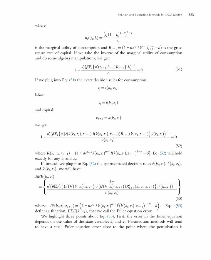
where

uc0 ct, ltð Þ¼ cτt 1� ltð Þ1�τ� �1�η

ct

is the marginal utility of consumption and Rt+1¼ 1+ αezt +1kα�1t l1�α

t+1 �δ� �

is the gross

return rate of capital. If we take the inverse of the marginal utility of consumption

and do some algebra manipulations, we get:

1�u0c βt u0c ct+1, lt+1ð ÞRt+1

� , lt

� ��1

ct¼ 0 (51)

If we plug into Eq. (51) the exact decision rules for consumption:

ct ¼ c kt,ztð Þ,labor

lt ¼ l kt,ztð Þand capital:

kt+1¼ k kt,ztð Þwe get:

1�u0c βt u0c c k kt ,ztð Þ,zt+1ð Þ, l k kt ,ztð Þ,zt+1ð Þð ÞRt+1 kt ,zt ,zt+1ð Þ� , l kt ,ztð Þ� ��1

c kt,ztð Þ ¼ 0

(52)

where R kt,zt,zt+1ð Þ¼ 1+ αezt+1k kt ,ztð Þα�1l k kt ,ztð Þ,zt+1ð Þ1�α�δ

� �. Eq. (52) will hold

exactly for any kt and zt.

If, instead, we plug into Eq. (52) the approximated decision rules cj kt,ztð Þ, lj kt,ztð Þ,and kj kt,ztð Þ, we will have:EEE kt,ztð Þ

¼1�

u0c βt u0c cj kj k

jt ,zt

� �,zt+1

� �, lj kj kt ,ztð Þ,zt+1ð Þ� �

Rjt+1 kt ,zt ,zt+1ð Þ�

, lj kt ,ztð Þ� ��1

cj kt,ztð Þ

8<:

9=;(53)

where Rj kt,zt,zt+1ð Þ¼ 1+ αezt+1kj kt ,ztð Þα�1li ki kt ,ztð Þ,zt+1

� �1�α�δ� �

. Eq. (53)

defines a function, EEE kt,ztð Þ, that we call the Euler equation error.

We highlight three points about Eq. (53). First, the error in the Euler equation

depends on the value of the state variables kt and zt. Perturbation methods will tend

to have a small Euler equation error close to the point where the perturbation is


undertaken and a larger Euler equation error farther from it. In contrast, projection

methods will deliver a more uniform Euler equation error across Ω. Consequently,researchers have found it useful to summarize the Euler equation error. Proposals include

the mean of the Euler equation error (either a simple average or using some estimate of

the ergodic distribution of state variablesad) or the maximum of the Euler equation error

in some region of Ω. Second, due to the algebraic transformation that we took on the

Euler equation, EEE kt,ztð Þ is expressed in consumption units, which have a meaningful

economic interpretation as the relative optimization error incurred by the use of the

approximated policy rule (Judd and Guu, 1997). For instance, if EEE kt,ztð Þ¼ 0:01, thenthe agent is making a $1 mistake for each $100 spent. In comparison, EEE kt,ztð Þ¼ 1e�6

implies that the agent is making a 1 cent mistake for each 1million spent. Third, the Euler

equation error is also important because we know that, under certain conditions, the

approximation error of the decision rule is of the same order of magnitude as the size

of the Euler equation error. Correspondingly, the change in welfare is of the square order

of the Euler equation error. Furthermore, the constants involved in these error bounds

can be related to model primitives (Santos, 2000). Unfortunately, in some DSGE models

it can be difficult to use algebraic transformations to achieve an expression for the Euler

equation error that is interpretable as consumption units (or other natural economic unit).

Following the convention in the literature, we plot in Fig. 13, the log10 EEE kt,ztð Þj jof the stochastic neoclassical growth model from Section 5.6. Taking the log10 eases

reading: a value of -3 means $1 mistake for each $1000, a value of -4 a $1 mistake for

each $10,000, and so on. Fig. 13 shows five lines, one for each value of productivity.

As we hinted when we described the Chebyshev-collocation projection method, this

accuracy is outstanding.

To compare this performance of Chebyshev-collocation with other solution

methods, we reproduce, in Figs. 14 and 15, results from Aruoba et al. (2006). That paper

uses the same stochastic neoclassical growth model with only a slightly different calibra-

tion (plus a few smaller details about how to handle zt). Both figures display a transversal

cut of the Euler equation errors when zt ¼ 0 and for values of capital between 70% and

130% of its steady-state value (23.14).

In Fig. 14, we plot the results for a first-order perturbation (in levels and in logs), a

second-order perturbation, and a fifth-order perturbation. First, perturbations have smal-

ler errors around the steady-state value of capital and deteriorate away from it. Second,

there is a considerable improvement when we go from a first- to a second-order approx-

imation. Third, a fifth-order approximation displays a great performance even 30% away

from the steady state.

ad Using the ergodic distribution has the complication that we may not have access to it, since it is derived

from the solution of the model, the object we are searching for. See Aruoba et al. (2006) for suggestions on

how to handle this issue.


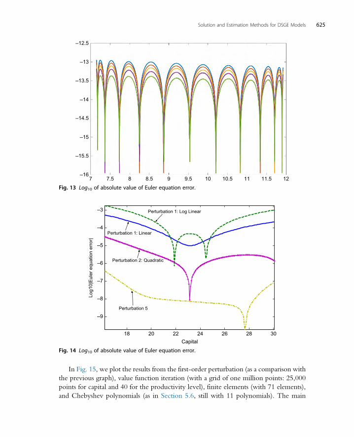
In Fig. 15, we plot the results from the first-order perturbation (as a comparison with

the previous graph), value function iteration (with a grid of one million points: 25,000

points for capital and 40 for the productivity level), finite elements (with 71 elements),

and Chebyshev polynomials (as in Section 5.6, still with 11 polynomials). The main

18 20 22 24 26 28 30

–9

–8

–7

–6

–5

–4

–3

Capital

Log1

0|E

uler

equ

atio

n er

ror|

Perturbation 1: Log Linear

Perturbation 1: Linear

Perturbation 2: Quadratic

Perturbation 5

Fig. 14 Log10 of absolute value of Euler equation error.

7.5 8 8.5 9 9.5 10 10.5 11 11.5 127–16

–15.5

–15

–14.5

–14

–13.5

–13

–12.5



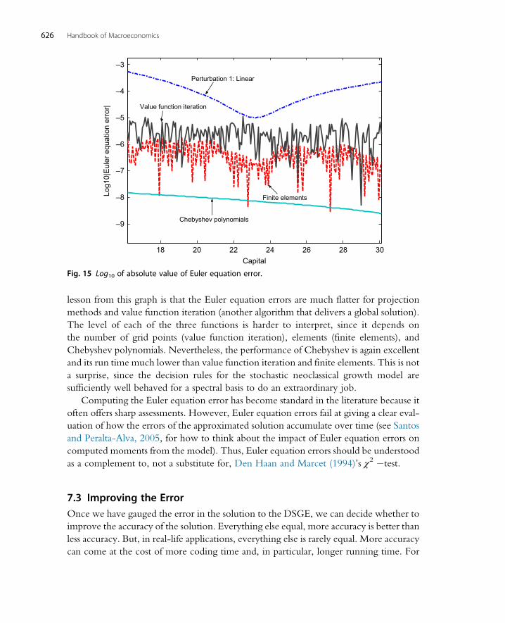
lesson from this graph is that the Euler equation errors are much flatter for projection

methods and value function iteration (another algorithm that delivers a global solution).

The level of each of the three functions is harder to interpret, since it depends on

the number of grid points (value function iteration), elements (finite elements), and

Chebyshev polynomials. Nevertheless, the performance of Chebyshev is again excellent

and its run time much lower than value function iteration and finite elements. This is not

a surprise, since the decision rules for the stochastic neoclassical growth model are

sufficiently well behaved for a spectral basis to do an extraordinary job.

Computing the Euler equation error has become standard in the literature because it

often offers sharp assessments. However, Euler equation errors fail at giving a clear eval-

uation of how the errors of the approximated solution accumulate over time (see Santos

and Peralta-Alva, 2005, for how to think about the impact of Euler equation errors on

computed moments from the model). Thus, Euler equation errors should be understood

as a complement to, not a substitute for, Den Haan and Marcet (1994)’s χ2 �test.

7.3 Improving the ErrorOnce we have gauged the error in the solution to the DSGE, we can decide whether to

improve the accuracy of the solution. Everything else equal, more accuracy is better than

less accuracy. But, in real-life applications, everything else is rarely equal. More accuracy

can come at the cost of more coding time and, in particular, longer running time. For

18 20 22 24 26 28 30

–9

–8

–7

–6

–5

–4

–3

Capital

Log1

0|E

uler

equ

atio

n er

ror|

Perturbation 1: Linear

Value function iteration

Chebyshev polynomials

Finite elements



example, in the exercise with the stochastic neoclassical growth model reported in

Fig. 15, we could subdivide the finite elements as much as we want and use modern sci-

entific libraries such as theGNU multiple precision arithmetic library to achieve any arbitrary

level of accuracy, but at the cost of longer running times andmorememory requirements.

The researcher must look at her needs and resources and, once inferior solution methods

are rejected, select those that best fit her goals.

But if the goal is indeed dependent on achieving additional accuracy, there are dif-

ferent possibilities available. If a perturbation is being used, we can increase the order of

the perturbation. If a projection method is being used, we can increase the number of

elements in the basis. The researcher can also explore changes of variables to make

the problem more linear or switch the solution method.

Once the error of the model has been assessed, we are finally ready to move to Part II

and see how the DSGE model can account for the observed data.

PART II. ESTIMATING DSGE MODELS8. CONFRONTING DSGE MODELS WITH DATA

The preceding sections discussed how to compute an approximate solution for a DSGE

model conditional on its parameterization. Part II focuses on determining the DSGE

model parameters based on the empirical evidence and assessing the model’s fit. More

specifically, we ask four fundamental questions: (i) How can one estimate the DSGE

model parameters from the observed macroeconomic time series? (ii) How well does

the estimated DSGE model capture salient features of the data? (iii) What are the quan-

titative implications of the estimated DSGE models with respect to, for instance, sources

of business cycle fluctuations, propagation of exogenous shocks, the effect of changes in

macroeconomic policies, and the future path of macroeconomic time series? (iv) How

should one construct measures of uncertainty for the parameters and the quantitative

implications of the DSGE model? To answer these questions, we begin by analytically

solving a stylized New Keynesian DSGEmodel in Section 8.1 and studying its properties

in Section 8.2. DSGEmodel-implied population moments, autocovariances, spectra, and

impulse response functions have sample analogs in the data, which are examined in

Section 8.3. Macroeconomic time series exhibit trends that may or may not be captured

by the DSGE model, which is discussed in Section 8.4.

Part II of this chapter assumes that the reader has some basic familiarity with econo-

metrics, at the level of a first-year PhD sequence in a US graduate program. With the

exception of Canova (2007) and DeJong and Dave (2007) there are no textbooks that

focus on the estimation of DSGE models. The literature has progressed quickly since

these two books were first written. The subsequent sections contain, in addition to a

critical introduction to “standard methods,” an overview of the most recent develop-

ments in the literature, which include identification conditions for DSGE models,


identification-robust frequentist inference, and sequential Monte Carlo techniques for

Bayesian analysis. Unlike the recent monograph byHerbst and Schorfheide (2015) which

focuses on Bayesian computations, Part II of this chapter also contains extensive discus-

sions of the consequences of misspecification for econometric inference and covers fre-

quentist methods.

8.1 A Stylized DSGE ModelThroughout Part II we consider a stylized New Keynesian DSGE model in its loglinear-

ized form.ae This model shares many of the features of its more realistic siblings that have

been estimated in the literature. It is a stripped-down version of the model developed in

the work by Christiano et al. (2005) and Smets andWouters (2003). The specific version

presented below is taken from Del Negro and Schorfheide (2008) and obtained by

imposing several parameter restrictions. It is not suitable to be confronted with actual

data, but it can be solved analytically, which is useful for the subsequent exposition.

For brevity, we refer to this model as the stylized DSGE model in the remainder of this

chapter.

The model economy consists of households, intermediate goods producers, final

goods producers, a monetary policy authority, and a fiscal authority. Macroeconomic

fluctuations are generated by four exogenous processes: a technology growth shock,

zt, a shock that generates shifts in the preference for leisure, ϕt, a price markup shock,

λt, and a monetary policy shock ER,t. We assume that the level of productivity Zt in

the economy is evolving exogenously according to a random walk with drift:

logZt ¼ logγ + logZt�1 + zt, zt ¼ ρzzt�1 + σzEz, t: (54)

The productivity processZt induces a stochastic trend in outputXt and real wagesWt. To

facilitate the model solution, it is useful to detrend output and real wages by the level of

technology, defining xt ¼ Xt/Zt and wt ¼Wt/Zt, respectively. In terms of the detrended

variables, the model has the following steady state:

�x¼ x*, �w ¼ lsh¼ 1

1+ λ, π ¼ π*, �R¼ π*

γ

β: (55)

Here x* and π* are free parameters. The latter can be interpreted as the central bank’s

target inflation rate, whereas the former can in principle be derived from the weight

on leisure in the households’ utility function. The steady-state real wage �w is equal to

the steady-state labor share lsh. The parameter λ can be interpreted as the steady-state

markup charged by the monopolistically competitive intermediate goods producers, βis the discount factor of the households, and γ is the growth rate of technology. Under

the assumption that the production technology is linear in labor and labor is the only

ae See Sections 4.1 and 4.5 for how to think about loglinearizations as a first-order perturbations.


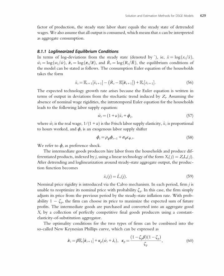
factor of production, the steady state labor share equals the steady state of detrended

wages.We also assume that all output is consumed, whichmeans that x can be interpreted

as aggregate consumption.

8.1.1 Loglinearized Equilibrium ConditionsIn terms of log-deviations from the steady state (denoted by ^), ie, x¼ logðxt=�xÞ,wt ¼ logðwt=�wÞ, π t ¼ logðπt=πÞ, and Rt ¼ logðRt= �RÞ, the equilibrium conditions of

the model can be stated as follows. The consumption Euler equation of the households

takes the form

xt ¼t+1½xt+1�� Rt�½π t+1��

+t½zt+1�: (56)

The expected technology growth rate arises because the Euler equation is written in

terms of output in deviations from the stochastic trend induced by Zt. Assuming the

absence of nominal wage rigidities, the intratemporal Euler equation for the households

leads to the following labor supply equation:

wt ¼ð1+ νÞxt +ϕt, (57)

where wt is the real wage, 1/(1 + ν) is the Frisch labor supply elasticity, xt is proportionalto hours worked, and ϕt is an exogenous labor supply shifter

ϕt ¼ ρϕϕt�1 + σϕEϕ, t: (58)

We refer to ϕt as preference shock.

The intermediate goods producers hire labor from the households and produce dif-

ferentiated products, indexed by j, using a linear technology of the form Xt( j)¼ ZtLt( j).

After detrending and loglinearization around steady-state aggregate output, the produc-

tion function becomes

xtðjÞ¼ L tðjÞ: (59)

Nominal price rigidity is introduced via the Calvo mechanism. In each period, firm j is

unable to reoptimize its nominal price with probability ζp. In this case, the firm simply

adjusts its price from the previous period by the steady-state inflation rate. With prob-

ability 1 � ζp, the firm can choose its price to maximize the expected sum of future

profits. The intermediate goods are purchased and converted into an aggregate good

Xt by a collection of perfectly competitive final goods producers using a constant-

elasticity-of-substitution aggregator.

The optimality conditions for the two types of firms can be combined into the

so-called New Keynesian Phillips curve, which can be expressed as

π t ¼ βt½π t+1�+ κpðwt + λtÞ, κp¼ð1�ζpβÞð1� ζpÞ

ζp, (60)


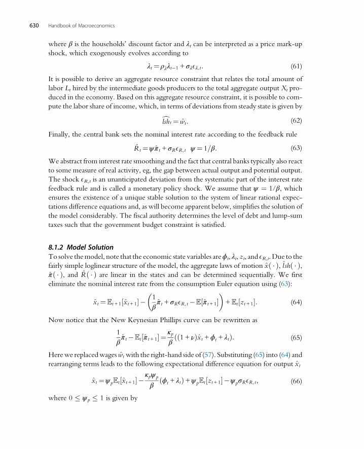
where β is the households’ discount factor and λt can be interpreted as a price mark-up

shock, which exogenously evolves according to

λt ¼ ρλλt�1 + σλEλ, t: (61)

It is possible to derive an aggregate resource constraint that relates the total amount of

labor Lt hired by the intermediate goods producers to the total aggregate output Xt pro-

duced in the economy. Based on this aggregate resource constraint, it is possible to com-

pute the labor share of income, which, in terms of deviations from steady state is given by

clsht ¼ wt: (62)

Finally, the central bank sets the nominal interest rate according to the feedback rule

Rt ¼ψπ t + σRER, t ψ ¼ 1=β: (63)

We abstract from interest rate smoothing and the fact that central banks typically also react

to some measure of real activity, eg, the gap between actual output and potential output.

The shock ER,t is an unanticipated deviation from the systematic part of the interest rate

feedback rule and is called a monetary policy shock. We assume that ψ ¼ 1/β, whichensures the existence of a unique stable solution to the system of linear rational expec-

tations difference equations and, as will become apparent below, simplifies the solution of

the model considerably. The fiscal authority determines the level of debt and lump-sum

taxes such that the government budget constraint is satisfied.

8.1.2 Model SolutionTo solve themodel, note that the economic state variables areϕt, λt, zt, and ER,t. Due to the

fairly simple loglinear structure of the model, the aggregate laws of motion xð � Þ, l shð � Þ,πð � Þ, and Rð � Þ are linear in the states and can be determined sequentially. We first

eliminate the nominal interest rate from the consumption Euler equation using (63):

xt ¼t+1½xt+1�� 1

βπ t + σRER, t�½π t+1�

�+t½zt+1�: (64)

Now notice that the New Keynesian Phillips curve can be rewritten as

1

βπ t�t½π t+1� ¼ κp

βð1+ νÞxt +ϕt + λtð Þ: (65)

Herewe replacedwages wt with the right-hand side of (57). Substituting (65) into (64) and

rearranging terms leads to the following expectational difference equation for output xt

xt ¼ψ pt½xt+1��κpψp

βðϕt + λtÞ+ψ pt½zt+1��ψpσRER, t, (66)

where 0 � ψp � 1 is given by


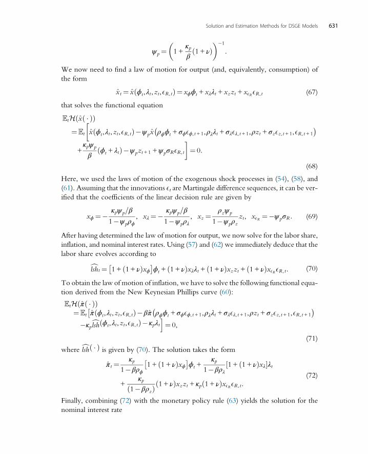
ψp¼ 1+κpβð1+ νÞ

��1

:

We now need to find a law of motion for output (and, equivalently, consumption) of

the form

xt ¼ x ϕt,λt,zt,ER, tð Þ¼ xϕϕt + xλλt + xzzt + xERER, t (67)

that solves the functional equation

tH xð � Þð Þ¼t x ϕt,λt,zt,ER, tð Þ�ψ px ρϕϕt + σϕEϕ, t+1,ρλλt + σλEλ, t+1,ρzt + σzEz, t+1,ER, t+1

� ��

+κpψ p

βðϕt + λtÞ�ψ pzt+1 +ψpσRER, t

¼ 0:

(68)

Here, we used the laws of motion of the exogenous shock processes in (54), (58), and

(61). Assuming that the innovations Et are Martingale difference sequences, it can be ver-

ified that the coefficients of the linear decision rule are given by

xϕ¼� κpψ p=β

1�ψ pρϕ, xλ¼� κpψp=β

1�ψ pρλ, xz ¼

ρzψ p

1�ψpρzzt, xER ¼�ψ pσR: (69)

After having determined the law of motion for output, we now solve for the labor share,

inflation, and nominal interest rates. Using (57) and (62) we immediately deduce that the

labor share evolves according to

clsht ¼ 1+ ð1+ νÞxϕ� �

ϕt + ð1+ νÞxλλt + ð1+ νÞxzzt + ð1+ νÞxERER, t: (70)

To obtain the law of motion of inflation, we have to solve the following functional equa-

tion derived from the New Keynesian Phillips curve (60):

tH πð � Þð Þ¼t π ϕt,λt,zt,ER, tð Þ�βπ ρϕϕt + σϕEϕ, t+1,ρλλt + σλEλ, t+1,ρzt + σzEz, t+1,ER, t+1

� ��κpclsh ϕt,λt,zt,ER, tð Þ�κpλt

i¼ 0,

(71)

where clshð � Þ is given by (70). The solution takes the form

π t ¼ κp1�βρϕ

1+ ð1+ νÞxϕ� �

ϕt +κp

1�βρλ1+ ð1+ νÞxλ½ �λt

+κp

ð1�βρzÞð1+ νÞxzzt + κpð1+ νÞxERER, t:

(72)

Finally, combining (72) with the monetary policy rule (63) yields the solution for the

nominal interest rate


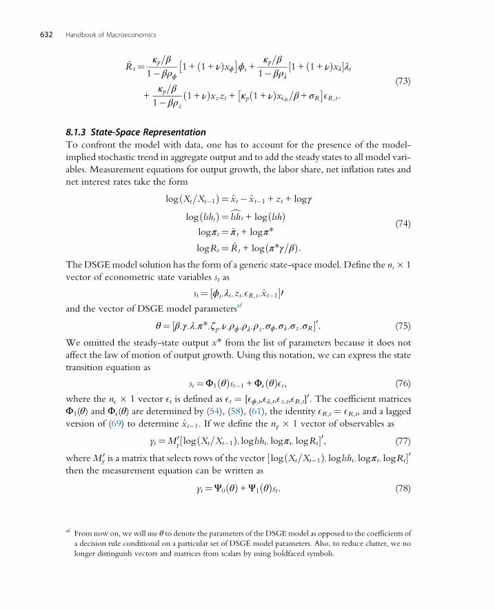
Rt ¼ κp=β

1�βρϕ1+ ð1+ νÞxϕ� �

ϕt +κp=β

1�βρλ1+ ð1+ νÞxλ½ �λt

+κp=β

1�βρzð1+ νÞxzzt + κpð1+ νÞxER=β+ σR

� �ER, t:

(73)

8.1.3 State-Space RepresentationTo confront the model with data, one has to account for the presence of the model-

implied stochastic trend in aggregate output and to add the steady states to all model vari-

ables. Measurement equations for output growth, the labor share, net inflation rates and

net interest rates take the form

logðXt=Xt�1Þ¼ xt� xt�1 + zt + logγ

logðlshtÞ¼clsht + logðlshÞlogπt ¼ π t + logπ*

logRt ¼ Rt + logðπ*γ=βÞ:

(74)

The DSGEmodel solution has the form of a generic state-space model. Define the ns� 1

vector of econometric state variables st as

st ¼ ½ϕt ,λt ,zt ,ER, t , xt�1�0and the vector of DSGE model parametersaf

θ¼ ½β,γ,λ,π*,ζp,ν,ρϕ,ρλ,ρz,σϕ,σλ,σz,σR�0: (75)

We omitted the steady-state output x* from the list of parameters because it does not

affect the law of motion of output growth. Using this notation, we can express the state

transition equation as

st ¼Φ1ðθÞst�1 +ΦEðθÞEt, (76)

where the nE � 1 vector Et is defined as Et ¼ [Eϕ,t,Eλ,t,Ez,t,ER,t]0. The coefficient matrices

Φ1(θ) and ΦE(θ) are determined by (54), (58), (61), the identity ER,t ¼ ER,t, and a lagged

version of (69) to determine xt�1. If we define the ny � 1 vector of observables as

yt ¼M 0y½ logðXt=Xt�1Þ, log lsht , logπt , logRt�0, (77)

whereMy0 is a matrix that selects rows of the vector ½ logðXt=Xt�1Þ, log lsht , logπt , logRt�0

then the measurement equation can be written as

yt ¼Ψ0ðθÞ+Ψ1ðθÞst: (78)

af From now on, we will use θ to denote the parameters of the DSGEmodel as opposed to the coefficients of

a decision rule conditional on a particular set of DSGE model parameters. Also, to reduce clutter, we no

longer distinguish vectors and matrices from scalars by using boldfaced symbols.


The coefficient matricesΨ0(θ) andΨ1(θ) can be obtained from (74), the equilibrium law

of motion for the detrended model variables given by (69), (70), (72), and (73). They are

summarized in Table 4.

The state-space representation of the DSGE model given by (76) and (78) provides

the basis for the subsequent econometric analysis. It characterizes the joint distribution of

the observables yt and the state variables st conditional on the DSGE model parameters θ

pðY1:T ,S1:T jθÞ¼Z YT

t¼1

pðytjst,θÞpðstjst�1,θÞ !

pðs0jθÞds0, (79)

where Y1:t ¼ {y1,…,yt} and S1:t ¼ {s1,…,st}. Because the states are (at least partially)

unobserved, we will often work with the marginal distribution of the observables

defined as

pðY1:T jθÞ¼Z

pðY1:T ,S1:T jθÞdS1:T : (80)

As a function of θ the density p(Y1:Tjθ) is called the likelihood function. It plays a centralrole in econometric inference and its evaluation will be discussed in detail in Section 10.

Remark 28 First, it is important to distinguish economic state variables, namely, ϕt, λt, zt,and ER,t, that are relevant for the agents’ intertemporal optimization problems, from the

econometric state variables st, which are used to cast the DSGE model solution into the

state-space form given by (76) and (78). The economic state variables of our simple model

are all exogenous. As we have seen in Section 4.3, the vector of state variables of a richer

DSGE model also may include one or more endogenous variables, eg, the capital stock.

Second, output growth in the measurement equation could be replaced by the level of

output. This would require adding x* to the parameter vector θ, eliminating xt�1 from st,

adding logZt=γt to st, and accounting for the deterministic trend component ð logγÞt inlog output in the measurement equation. Third, the measurement Eq. (78) could be aug-

mented by measurement errors. Fourth, if a DSGE model is solved with a higher-order

perturbation or projection method, then, depending on how exactly the state vector st is

defined, the state-transition Eq. (76), the measurement Eq. (78), or both are nonlinear.

8.2 Model ImplicationsOnce we specify a distribution for the innovation vector Et the probability distribution ofthe DSGE model variables is fully determined. Recall that the innovation standard

deviations were absorbed into the definition of the matrix ΦE(θ) in (76). For the sake

of concreteness, we assume that

Et � iidNð0, IÞ, (81)

where I denotes the identity matrix. Based on the probabilistic structure of the DSGE

model, we can derive a number of implications from the DSGE model that will later


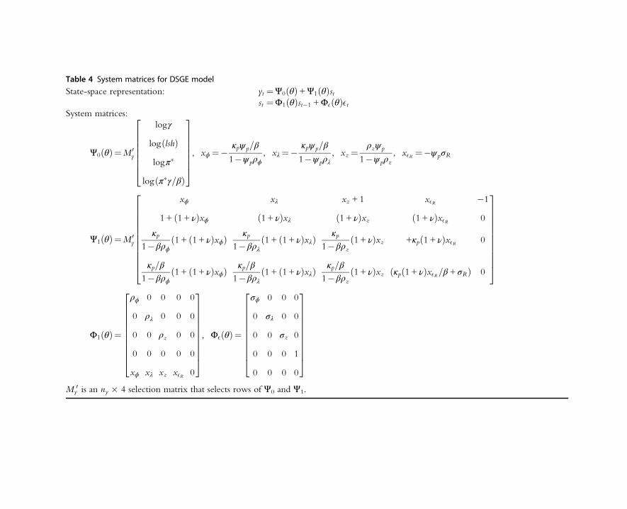
Table 4 System matrices for DSGE model

State-space representation: yt ¼Ψ0ðθÞ+Ψ1ðθÞstst ¼Φ1ðθÞst�1 +ΦEðθÞEt

System matrices:

Ψ0ðθÞ¼M 0y

logγ

logðlshÞlogπ�

logðπ�γ=βÞ

26666664

37777775, xϕ ¼� κpψ p=β

1�ψ pρϕ, xλ ¼� κpψ p=β

1�ψ pρλ, xz ¼

ρzψ p

1�ψ pρz, xER ¼�ψ pσR

Ψ1ðθÞ¼M 0y

xϕ xλ xz +1 xER �1

1+ ð1+ νÞxϕ ð1+ νÞxλ ð1+ νÞxz ð1+ νÞxER 0

κp1�βρϕ

ð1+ ð1+ νÞxϕÞ κp1�βρλ

ð1+ ð1+ νÞxλÞ κp1�βρz

ð1+ νÞxz +κpð1+ νÞxER 0

κp=β

1�βρϕð1+ ð1+ νÞxϕÞ κp=β

1�βρλð1+ ð1+ νÞxλÞ κp=β

1�βρzð1+ νÞxz ðκpð1+ νÞxER=β+ σRÞ 0

266666666664

377777777775

Φ1ðθÞ¼

ρϕ 0 0 0 0

0 ρλ 0 0 0

0 0 ρz 0 0

0 0 0 0 0

xϕ xλ xz xER 0

26666666664

37777777775, ΦEðθÞ¼

σϕ 0 0 0

0 σλ 0 0

0 0 σz 0

0 0 0 1

0 0 0 0

26666666664

37777777775

My0 is an ny � 4 selection matrix that selects rows of Ψ0 and Ψ1.

be used to construct estimators of the parameter vector θ and evaluate the fit of themodel.

For now, we fix θ to the values listed in Table 5.

8.2.1 Autocovariances and Forecast Error VariancesDSGE models are widely used for business cycle analysis. In this regard, the model-

implied variances, autocorrelations, and cross-correlations are important objects. For

linear DSGE models it is straightforward to compute the autocovariance function from

the state-space representation given by (76) and (78).ag Using the notation

ΓyyðhÞ¼½ytyt�h�, ΓssðhÞ¼½stst�h�, and ΓysðhÞ¼½yts0t�h�and the assumption that ½EtEt0� ¼ I , we can express the autocovariance matrix of st as the

solution to the following Lyapunov equation:ah

Γssð0Þ¼Φ1Γssð0ÞΦ10 +ΦEΦE0: (82)

Once the covariance matrix of st has been determined, it is straightforward to compute

the autocovariance matrices for h 6¼ 0 according to

ΓssðhÞ¼Φh1Γssð0Þ: (83)

Finally, using the measurement Eq. (78), we deduce that

ΓyyðhÞ¼Ψ1ΓssðhÞΨ01, ΓysðhÞ¼Ψ1ΓssðhÞ: (84)

Table 5 Parameter values for stylized DSGE modelParameter Value Parameter Value

β 1/1.01 γ expð0:005Þλ 0.15 π* expð0:005Þζp 0.65 ν 0

ρϕ 0.94 ρλ 0.88

ρz 0.13

σϕ 0.01 σλ 0.01

σz 0.01 σR 0.01

ag For the parameters in Table 5, the largest (in absolute value) eigenvalue of the matrix Φ1(θ) in (76) is less

than one, which implies that the VAR(1) law of motion for st is covariance stationary.ah Efficient numerical routines to solve Lyapunov equations are readily available in many software packages,

eg, the function dylap in MATLAB.


Correlations can be easily computed by normalizing the entries of the autocovariance

matrices using the respective standard deviations. Fig. 16 shows the model-implied auto-

correlation function of output growth and the cross-correlations of output growth with

the labor share, inflation, and interest rates as a function of the temporal shift h.

The law of motion for the state vector st can also be expressed as the infinite-order

vector moving average (MA) process

yt ¼Ψ0 +Ψ1

X∞s¼0

Φs1ΦEEt�s: (85)

Based on the moving average representation, it is straightforward to compute the

h-step-ahead forecast error, which is given by

etjt�h ¼ yt�t�h½yt� ¼Ψ1

Xh�1

s¼0

Φs1ΦEEt�s: (86)

The h-step-ahead forecast error covariance matrix is given by

½etjt�he0tjt�h� ¼Ψ1

Xh�1

s¼0

Φs1ΦEΦ0

EΦs01

!Ψ0

1 with limh!∞

½etjt�he0tjt�h� ¼Γssð0Þ: (87)

Under the assumption that ½EtE0t� ¼ I , it is possible to decompose the forecast error

covariance matrix as follows. Let I( j ) be defined by setting all but the j-th diagonal

element of the identity matrix I to zero. Then we can write

I ¼XnEj¼1

I ðjÞ: (88)

Corr (log(Xt/Xt−1), log(Xt−h/Xt−h−1)) Corr (log(Xt/Xt−1), log(Zt−h))

Fig. 16 Autocorrelations. Notes: Right panel: correlations of output growth with labor share (solid),inflation (dotted), and interest rates (dashed).


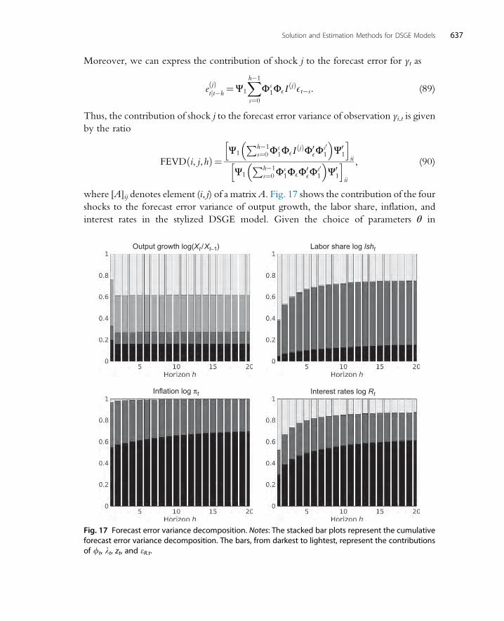
Moreover, we can express the contribution of shock j to the forecast error for yt as

eðjÞtjt�h

¼Ψ1

Xh�1

s¼0

Φs1ΦEI

ðjÞEt�s: (89)

Thus, the contribution of shock j to the forecast error variance of observation yi,t is given

by the ratio

FEVDði, j,hÞ¼Ψ1

Ph�1s¼0Φ

s1ΦEI

ðjÞΦ0EΦ

s01

� �Ψ0

1

h iii

Ψ1

Ph�1s¼0Φ

s1ΦEΦ0

EΦs01

� �Ψ0

1

h iii

, (90)

where [A]ij denotes element (i, j) of a matrixA. Fig. 17 shows the contribution of the four

shocks to the forecast error variance of output growth, the labor share, inflation, and

interest rates in the stylized DSGE model. Given the choice of parameters θ in

Output growth log(Xt /Xt−1)

Inflation log πt Interest rates log Rt

Labor share log lsht

Fig. 17 Forecast error variance decomposition. Notes: The stacked bar plots represent the cumulativeforecast error variance decomposition. The bars, from darkest to lightest, represent the contributionsof ft, lt, zt, and eR.t.


Table 5, most of the variation in output growth is due to the technology and the mon-

etary policy shocks. The labor share fluctuations are dominated by the mark-up shock λt,in particular in the long run. Inflation and interest rate movements are strongly influenced

by the preference shock ϕt and the mark-up shock λt.

8.2.2 SpectrumInstead of studying DSGE model implications over different forecasting horizons, one can

also consider different frequency bands. There is a long tradition of frequency domain anal-

ysis in the time series literature. A classic reference is Priestley (1981). We start with a brief

discussion of the linear cyclical model, whichwill be useful for interpreting some of the for-

mulas presented subsequently. Suppose that yt is a scalar time series that follows the process

yt ¼ 2Xmj¼1

aj cosθj cosðωjtÞ� sinθj sinðωjtÞ� �

, (91)

where θj� iidU[�π,π] and 0�ωj�ωj+1� π. The random variables θj cause a phase shiftof the cycle and are assumed to be determined in the infinite past. In a nutshell, the model

in (91) expresses the variable yt as the sum of sine and cosine waves that differ in their

frequency. The interpretation of the ωj’s depends on the length of the period t. Suppose

the model is designed for quarterly data and ωj ¼ (2π)/32. This means that it takes

32 periods to complete the cycle. Business cycles typically comprise cycles that have

a duration of 8–32 quarters, which would correspond to ωj 2 [0.196, 0.785] for

quarterly t.

Using Euler’s formula, we rewrite the cyclical model in terms of an exponential

function:

yt ¼Xmj¼�m

AðωjÞeiωj t, (92)

where ω�j ¼ �ωj, i¼ffiffiffiffiffiffiffi�1

p, and

AðωjÞ¼ ajðcosθjjj + i sinθjjjÞ if j> 0

ajðcosθjjj � i sinθjjjÞ if j< 0

�(93)

It can be verified that expressions (91) and (92) are identical. The function A(ωj) captures

the amplitude of cycles with frequency ωj.

The spectral distribution function of yt on the interval ω 2 (�π,π] is defined as

FyyðωÞ¼Xmj¼�m

½AðωjÞAðωjÞ�fωj �ωg, (94)

where fωj �ωg denotes the indicator function that is one if ωj�ω and �z¼ x� iy is the

complex conjugate of z¼ x + iy. If Fyy(ω) is differentiable with respect toω, then we candefine the spectral density function as


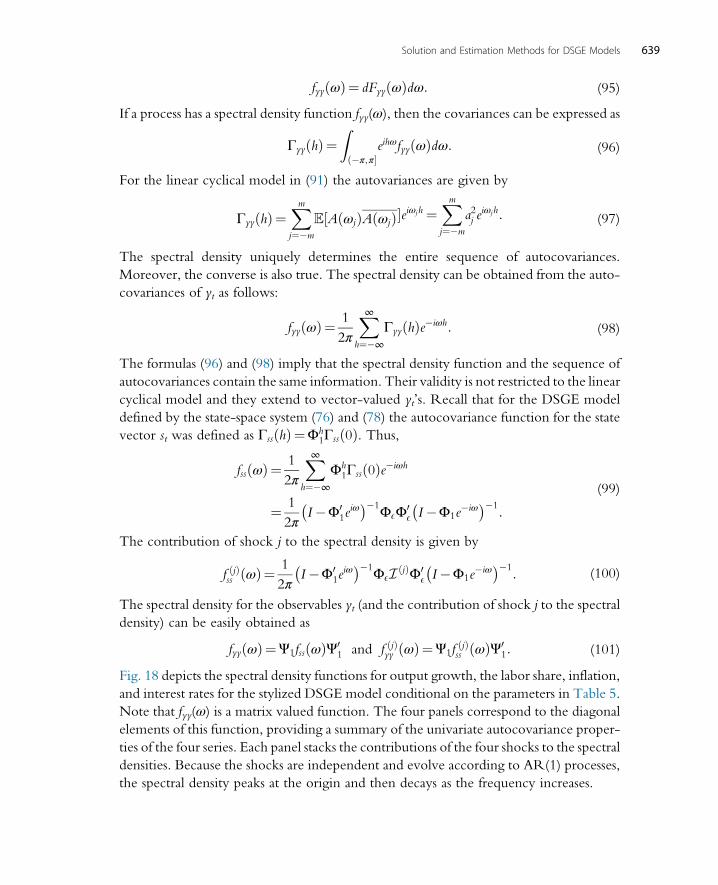
fyyðωÞ¼ dFyyðωÞdω: (95)

If a process has a spectral density function fyy(ω), then the covariances can be expressed as

ΓyyðhÞ¼Zð�π,π�

eihωfyyðωÞdω: (96)

For the linear cyclical model in (91) the autovariances are given by

ΓyyðhÞ¼Xmj¼�m

½AðωjÞAðωjÞ�eiωjh¼Xmj¼�m

a2j eiωjh: (97)

The spectral density uniquely determines the entire sequence of autocovariances.

Moreover, the converse is also true. The spectral density can be obtained from the auto-

covariances of yt as follows:

fyyðωÞ¼ 1

2π

X∞h¼�∞

ΓyyðhÞe�iωh: (98)

The formulas (96) and (98) imply that the spectral density function and the sequence of

autocovariances contain the same information. Their validity is not restricted to the linear

cyclical model and they extend to vector-valued yt’s. Recall that for the DSGE model

defined by the state-space system (76) and (78) the autocovariance function for the state

vector st was defined as ΓssðhÞ¼Φh1Γssð0Þ. Thus,

fssðωÞ¼ 1

2π

X∞h¼�∞

Φh1Γssð0Þe�iωh

¼ 1

2πI�Φ0

1eiω

� ��1ΦEΦ0E I�Φ1e

�iω� ��1

:

(99)

The contribution of shock j to the spectral density is given by

f ðjÞss ðωÞ¼ 1

2πI �Φ0

1eiω

� ��1ΦEIðjÞΦ0E I�Φ1e

�iω� ��1

: (100)

The spectral density for the observables yt (and the contribution of shock j to the spectral

density) can be easily obtained as

fyyðωÞ¼Ψ1fssðωÞΨ01 and f ðjÞyy ðωÞ¼Ψ1f

ðjÞss ðωÞΨ0

1: (101)

Fig. 18 depicts the spectral density functions for output growth, the labor share, inflation,

and interest rates for the stylized DSGE model conditional on the parameters in Table 5.

Note that fyy(ω) is a matrix valued function. The four panels correspond to the diagonal

elements of this function, providing a summary of the univariate autocovariance proper-

ties of the four series. Each panel stacks the contributions of the four shocks to the spectral

densities. Because the shocks are independent and evolve according to AR(1) processes,

the spectral density peaks at the origin and then decays as the frequency increases.


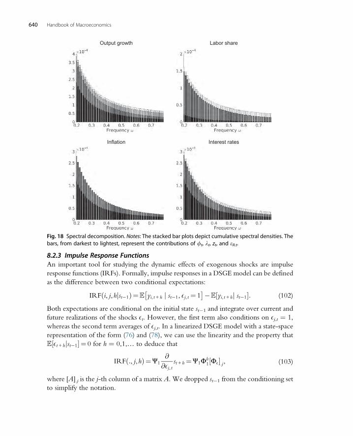
8.2.3 Impulse Response FunctionsAn important tool for studying the dynamic effects of exogenous shocks are impulse

response functions (IRFs). Formally, impulse responses in a DSGE model can be defined

as the difference between two conditional expectations:

IRFði, j,hjst�1Þ¼ yi, t+ h j st�1, Ej, t ¼ 1� �� yi, t+ hj st�1½ �: (102)

Both expectations are conditional on the initial state st�1 and integrate over current and

future realizations of the shocks Et. However, the first term also conditions on Ej,t ¼ 1,

whereas the second term averages of Ej,t. In a linearized DSGE model with a state-space

representation of the form (76) and (78), we can use the linearity and the property that

½Et+ hjst�1� ¼ 0 for h ¼ 0,1,… to deduce that

IRFð:, j,hÞ¼Ψ1

@

@Ej, tst+ h¼Ψ1Φh

1½ΦE�:j, (103)

where [A].j is the j-th column of a matrix A. We dropped st�1 from the conditioning set

to simplify the notation.

Output growth Labor share

Inflation Interest rates

Fig. 18 Spectral decomposition. Notes: The stacked bar plots depict cumulative spectral densities. Thebars, from darkest to lightest, represent the contributions of ft, lt, zt, and eR.t.


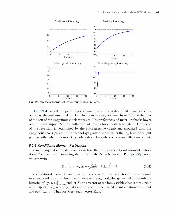
Fig. 19 depicts the impulse response functions for the stylized DSGE model of log

output to the four structural shocks, which can be easily obtained from (69) and the laws

of motion of the exogenous shock processes. The preference and mark-up shocks lower

output upon impact. Subsequently, output reverts back to its steady state. The speed

of the reversion is determined by the autoregressive coefficient associated with the

exogenous shock process. The technology growth shock raises the log level of output

permanently, whereas a monetary policy shock has only a one-period effect on output.

8.2.4 Conditional Moment RestrictionsThe intertemporal optimality conditions take the form of conditional moment restric-

tions. For instance, rearranging the terms in the New Keynesian Phillips (60) curve,

we can write

t�1 π t�1�βπ t� κpðclsht�1 + λt�1Þh i

¼ 0: (104)

The conditional moment condition can be converted into a vector of unconditional

moment conditions as follows. Let F t denote the sigma algebra generated by the infinite

histories of fyτ , sτ ,Eτgtτ¼�∞ and let Z�t be a vector of random variables that is measurable

with respect to F t, meaning that its value is determined based on information on current

and past (yt,st,Et). Then for every such vector Z�t�1,

Preference innov. ef,t Mark-up innov. el,t

Techn. growth innov. ez,t Monetary policy innov. eR,t

Fig. 19 Impulse responses of log output 100logðXt + h=XtÞ.


Z�t�1 π t�1�βπ t� κpðclsht�1 + λt�1Þ� �h i

¼ Z�t�1t�1 π t�1�βπ t� κpðclsht�1 + λt�1Þ

h ih i¼ 0,

(105)

where t�1½ � � ¼½ � jF t�1�.The moment conditions derived from the New Keynesian Phillips curve involve the

latent price mark-up shock λt, which will cause difficulties if one tries to use (105) in an

estimation objective function. Now consider the consumption Euler equation (56)

instead. Recall that the measurement equations imply that

xt� xt�1 + zt ¼ logXt� logXt�1� logγ and Rt ¼ logRt� logðπ*γ=βÞ:Thus, we can write

t�1 � logðXt=Xt�1Þ+ logRt�1� logπt� logð1=βÞ½ � ¼ 0: (106)

The terms γ and logπ* that appear in the steady-state formulas for the nominal interest

rate and inflation cancel and the conditional moment condition only depends on

observables and the model parameters, but not on latent variables. Finally, as long as

the monetary policy shock satisfies the martingale difference sequences property

t�1½ER, t� ¼ 0, we obtain from the monetary policy rule the condition that

t�1 logRt� logðγ=βÞ�ψ logπt�ð1�ψÞ logπ*½ � ¼ 0: (107)

Both (106) and (107) can be converted into an unconditional moment condition using an

F t�1 measurable random vector Zt�1 as in (105).

8.2.5 Analytical Calculation of Moments vs Simulation ApproximationsAs previously shown, formulas for autocovariance functions, spectra, and impulse

response functions for a linearized DSGE model can be derived analytically from the

state-space representation. These analytical expressions can then be numerically evalu-

ated for different vectors of parameter values θ. For DSGE models solved with pertur-

bation methods, there are also analytical formulas available that exploit a conditionally

linear structure of some perturbation solutions; see Andreasen et al. (2013). For a general

nonlinear DSGE model, the implied moments have to be computed using Monte Carlo

simulation. For instance, let Y*1:T denote a sequence of observations simulated from the

state-space representation of the DSGE model by drawing an initial state vector s0 and

innovations Et from their model-implied distributions, then

1

T

XTt¼1

y*t ��!a:s: ½yt�, (108)


provided that the DSGE model-implied yt is strictly stationary and ergodic.ai The down-

side of Monte Carlo approximations is that they are associated with a simulation error.

We will come back to this problem in Section 11.2, when we use simulation approxi-

mations of moments to construct estimators of θ.

8.3 Empirical AnalogsWe now examine sample analogs of the population moments derived from the state-

space representation of the DSGE model using US data. The time series were down-

loaded from the FRED database maintained by the Federal Reserve Bank of St. Louis

and we report the series labels in parentheses. For real aggregate output, we use quarterly,

seasonally adjusted GDP at the annual rate that has been pegged to 2009 dollars

(GDPC96). We turn GDP into growth rates by taking logs and then differencing.

The labor share is defined as Compensation of Employees (COE) divided by nominal

GDP (GDP). Both series are quarterly and seasonally adjusted at the annual rate. We

use the log labor share as the observable. Inflation rates are computed from the implicit

price deflator (GDPDEF) by taking log differences. Lastly, for the interest rate, we use the

Effective Federal Funds Rate (FEDFUNDS), which is monthly, and not seasonally

adjusted. Quarterly interest rates are obtained by taking averages of the monthly rates.

Throughout this section we focus on the post-Great Moderation and pre-Great

Recession period and restrict our sample from 1984:Q1 to 2007:Q4.

8.3.1 AutocovariancesThe sample analog of the population autocovariance Γyy(h) is defined as

ΓyyðhÞ¼ 1

T

XTt¼h

ðyt� μyÞðyt�h� μyÞ0, where μy¼1

T

XTt¼1

yt: (109)

Under suitable regularity conditions, eg, covariance stationarity of the vector process yt, a

sufficiently fast decay of the serial correlation in yt, and some bounds on higher-order

moments of yt, the sample autocovariance ΓyyðhÞ converges to the population autoco-

variance Γyy(h), satisfying a strong law of large numbers (SLLN) and a central limit

theorem (CLT).

If the object of interest is a sequence of autocovariance matrices, then it might

be more efficient to first estimate an auxiliary model and then convert the parameter esti-

mates of the auxiliary model into estimates of the autocovariance sequence. A natural

class of auxiliary models is provided by linear vector autoregressions (VARs). For

illustrative purposes consider the following VAR(1):

ai A sequence of random variables XT converges to a limit random variable X almost surely (a.s.) if the set of

trajectories for which XT !X has probability zero.


yt ¼Φ1yt�1 +Φ0 + ut, ut � iidð0,ΣÞ: (110)

The OLS estimator of Φ1 can be approximated by

Φ1¼ Γyyð1ÞΓ�1

yy ð0Þ+OpðT�1Þ, Σ¼ Γyyð0Þ� Γyyð1ÞΓ�1

yy ð0ÞΓ0yyð1Þ+OpðT�1Þ (111)

The Op(T�1) terms arise because the range of the summations in the definition of the

sample autocovariances in (109) and the definition of the OLS estimator are not exactly

the same.aj Suppose that now we plug the OLS estimator into the autocovariance for-

mulas associated with the VAR(1) (see (82) and (83)), then:

ΓV

yyð0Þ¼ Γyyð0Þ+OpðT�1Þ, ΓV

yyðhÞ¼ Γyyð1ÞΓ�1

yy ð0Þ� �h

Γyyð0Þ+OpðT�1Þ: (112)

Note that for h¼ 0,1 we obtain ΓV

yyð1Þ¼ Γyyð1Þ+OpðT�1Þ. For h> 1 the VAR(1) plug-

in estimate of the autocovariance matrix differs from the sample autocovariance matrix. If

the actual time series are well approximated by a VAR(1), then the plug-in autocovar-

iance estimate tends to be more efficient than the sample autocovariance estimate ΓyyðhÞ;see, for instance, Schorfheide (2005b).

In practice, a VAR(1) may be insufficient to capture the dynamics of a time series yt.

In this case the autocovariances can be obtained from a VAR(p)

yt ¼Φ1yt�1 +…+Φpyt�p +Φ0 + ut, ut � iidð0,ΣÞ: (113)

The appropriate lag length p can be determined with a model selection criterion, eg, the

Schwarz (1978) criterion, which is often called the Bayesian information criterion (BIC).

The notationally easiest way (but not the computationally fastest way) is to rewrite the

VAR(p) in companion form. This entails expressing the law of motion for the stacked

vector y�t ¼ ½y0t,y0t�1,…,y0t�p+1� as VAR(1):

y�t ¼Φ

�1y�t�1 +Φ

�0 + ~ut, ~ut � iidð0, Σ�Þ, (114)

where

Φ�1¼

Φ1 … Φp�1 Φp

In�n … 0n�n 0n�n

..

. . .. ..

. ...

0n�n … In�n 0n�n

266664

377775, Φ

�0¼

Φ0

0nðp�1Þ�1

" #,

E�t ¼Et

0nðp�1Þ�1

" #, Σ

� ¼ Σ 0n�nðp�1Þ0nðp�1Þ�n 0nðp�1Þ�nðp�1Þ

" #:

aj We say that a sequence of random variables is Op(T�1) if TXT is stochastically bounded as T !∞.


The autocovariances for y�t are then obtained by adjusting the VAR(1) formulas (112) to

y�t and reading off the desired submatrices that correspond to the autocovariance matrices

for yt using the selection matrix M0 ¼ [In,0n�n(p�1)] such that yt ¼M 0y�t.

We estimate a VAR for output growth, labor share, inflation, and interest rates.

The lag length p ¼ 1 is determined by the BIC. The left panel of Fig. 20 shows sample

cross-correlations (obtained from ΓyyðhÞ in (109)) between output growth and leads and

lags of the labor share, inflation, and interest rates, respectively. The right panel depicts

correlation functions derived from the estimated VAR(1). The two sets of correlation

functions are qualitatively similar but quantitatively different. Because the VAR model

is more parsimonious, the VAR-implied correlation functions are smoother.

8.3.2 SpectrumAn intuitively plausible estimate of the spectrum is the sample periodogram, defined as

f yyðωÞ¼1

2π

XT�1

h¼�T +1

ΓyyðhÞe�iωh¼ 1

2πΓyyð0Þ+

XT�1

h¼1

ðΓyyðhÞ+ ΓyyðhÞ0Þcosωh !

: (115)

While the sample periodogram is an asymptotically unbiased estimator of the population

spectral density, it is inconsistent because its variance does not vanish as the sample size

T !∞. A consistent estimator can be obtained by smoothing the sample periodogram

across adjacent frequencies. Define the fundamental frequencies

ωj ¼ j2π

T, j¼ 1,…,ðT �1Þ=2

and let K(x) denote a kernel function with the property thatRKðxÞdx¼ 1. A smoothed

periodogram can be defined as

Sample correlations VAR implied correlations

Fig. 20 Empirical cross-correlations Corr logðXt=Xt�1Þ, logZt�hð Þ. Notes: Each plot shows thecorrelation of output growth logðXt=Xt�1Þ with interest rates (solid), inflation (dashed), and thelabor share (dotted), respectively. Left panel: correlation functions are computed from sampleautocovariance matrices GyyðhÞ. Right panel: correlation functions are computed from estimatedVAR(1).


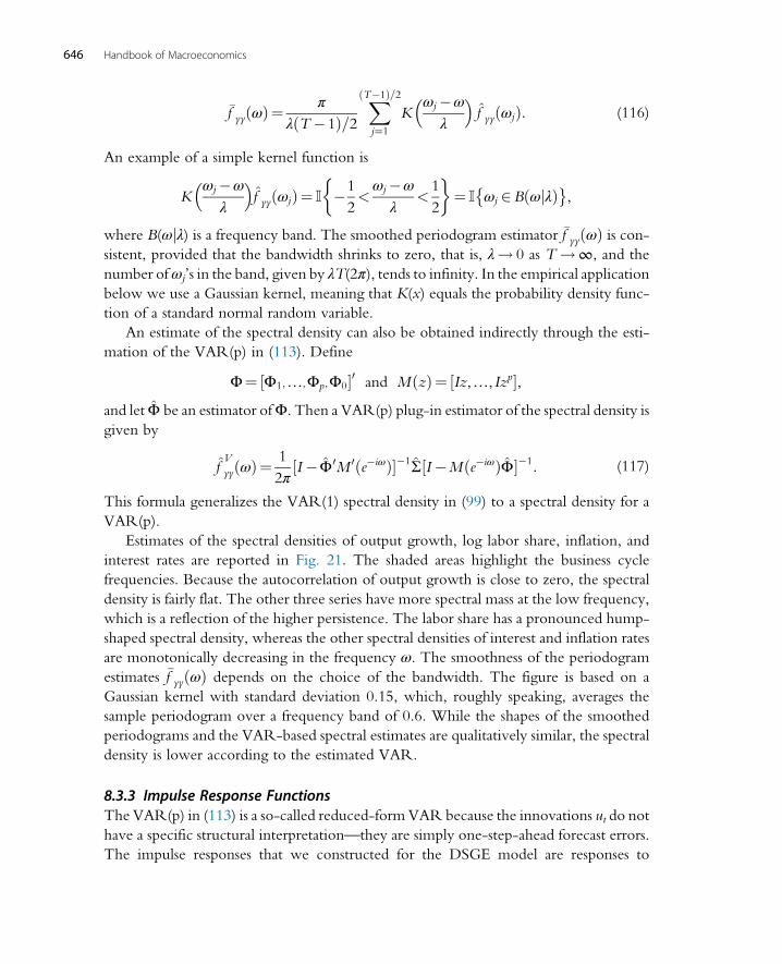
�f yyðωÞ¼π

λðT �1Þ=2XðT�1Þ=2

j¼1

Kωj�ω

λ

� �f yyðωjÞ: (116)

An example of a simple kernel function is

Kωj�ω

λ

� �f yyðωjÞ¼ �1

2<ωj�ω

λ<1

2

� �¼ ωj 2BðωjλÞ�

,

where B(ωjλ) is a frequency band. The smoothed periodogram estimator �f yyðωÞ is con-sistent, provided that the bandwidth shrinks to zero, that is, λ! 0 as T !∞, and the

number ofωj’s in the band, given by λT(2π), tends to infinity. In the empirical application

below we use a Gaussian kernel, meaning that K(x) equals the probability density func-

tion of a standard normal random variable.

An estimate of the spectral density can also be obtained indirectly through the esti-

mation of the VAR(p) in (113). Define

Φ¼ ½Φ1,…,Φp,Φ0�0 and MðzÞ¼ ½Iz,…, Izp�,and let Φ be an estimator ofΦ. Then a VAR(p) plug-in estimator of the spectral density is

given by

fV

yyðωÞ¼1

2π½I � Φ0M 0ðe�iωÞ��1Σ½I�Mðe�iωÞΦ��1: (117)

This formula generalizes the VAR(1) spectral density in (99) to a spectral density for a

VAR(p).

Estimates of the spectral densities of output growth, log labor share, inflation, and

interest rates are reported in Fig. 21. The shaded areas highlight the business cycle

frequencies. Because the autocorrelation of output growth is close to zero, the spectral

density is fairly flat. The other three series have more spectral mass at the low frequency,

which is a reflection of the higher persistence. The labor share has a pronounced hump-

shaped spectral density, whereas the other spectral densities of interest and inflation rates

are monotonically decreasing in the frequency ω. The smoothness of the periodogram

estimates �f yyðωÞ depends on the choice of the bandwidth. The figure is based on a

Gaussian kernel with standard deviation 0.15, which, roughly speaking, averages the

sample periodogram over a frequency band of 0.6. While the shapes of the smoothed

periodograms and the VAR-based spectral estimates are qualitatively similar, the spectral

density is lower according to the estimated VAR.

8.3.3 Impulse Response FunctionsThe VAR(p) in (113) is a so-called reduced-form VAR because the innovations ut do not

have a specific structural interpretation—they are simply one-step-ahead forecast errors.

The impulse responses that we constructed for the DSGE model are responses to


innovations in the structural shock innovations that contribute to the forecast error for

several observables simultaneously. In order to connect VAR-based impulse responses to

DSGE model-based responses, one has to link the one-step-ahead forecast errors to a

vector of structural innovations Et. We assume that

ut ¼ΦEEt ¼ΣtrΩEt, (118)

where Σtr is the unique lower-triangular Cholesky factor of Σwith nonnegative diagonal

elements, and Ω is an n � n orthogonal matrix satisfying ΩΩ0 ¼ I. The second equality

ensures that the covariance matrix of ut is preserved in the sense that

ΦEΦ0E¼ΣtrΩΩ0Σ0

tr ¼Σ: (119)

Output growth Labor share

Inflation Interest rates

Fig. 21 Empirical spectrum. Notes: The dotted lines are spectra computed from an estimated VAR(1);the solid lines are smoothed periodograms based on a Gaussian kernel with standard deviation 0.15.The shaded areas indicate business cycle frequencies (0.196–0.785).


By construction, the covariance matrix of the forecast error is invariant to the choice of

Ω, which implies that it is not possible to identify Ω from the data. In turn, much of the

literature on structural VARs reduces to arguments about an appropriate set of restric-

tions for the matrix Ω. Detailed surveys about the restrictions, or identification schemes,

that have been used in the literature to identify innovations to technology, monetary pol-

icy, government spending, and other exogenous shocks can be found, for instance, in

Cochrane (1994), Christiano et al. (1999), Stock and Watson (2001), and Ramey

(2016). Conditional on an estimate of the reduced-form coefficient matrices Φ and Σand an identification scheme for one or more columns of Ω, it is straightforward to

express the impulse response as

dIRFV ð:, j,hÞ¼ChðΦÞΣtr ½Ω�:j, (120)

where the moving average coefficient matrix ChðΦÞ can be obtained from the compan-

ion form representation of the VAR in (114):ChðΦÞ¼M 0Φ� h

1M withM0 ¼ [In,0n�n(p�1)].

For illustrative purposes, rather than conditioning the computation of impulse

response functions on a particular choice of Ω, we follow the recent literature on sign

restrictions; see Faust (1998), Canova and De Nicolo (2002), and Uhlig (2005). The

key idea of this literature is to restrict the matricesΩ to a setOðΦ,ΣÞ such that the implied

impulse response functions satisfy certain sign restrictions. This means that the magnitude

of the impulse responses are only set-identified. Using our estimated VAR(1) in output

growth, log labor share, inflation, and interest rates, we impose the condition that in

response to a contractionary monetary policy shock interest rates increase and inflation

is negative for four quarters. Without loss of generality, we can assume that the shocks are

ordered such that the first column ofΩ, denoted by q, captures the effect of the monetary

policy shock. Conditional on the reduced-form VAR coefficient estimates ðΦ, ΣÞ, wecan determine the set of unit-length vectors q such that the implied impulse responses

satisfy the sign restrictions. The bands depicted in Fig. 22 delimit the upper and lower

bounds of the estimated identified sets for the pointwise impulse responses of output,

labor share, inflation, and interest rates to a monetary policy shock. The sign restrictions

that are imposed on the monetary policy shock are not sufficiently strong to determine

the sign of the output and labor share responses to a monetary policy shock. Note that if a

researcher selects a particular q (possibly as a function of the reduced-form parameters Φand Σ), then the bands in the figure would reduce to a single line, which is exemplified by

the solid line in Fig. 22.

8.3.4 Conditional Moment RestrictionsThe unconditional moment restrictions derived from the equilibrium conditions of the

DSGE model discussed in Section 8.2.4 have sample analogs in which the population

expectations are replaced by sample averages. A complication arises if the moment


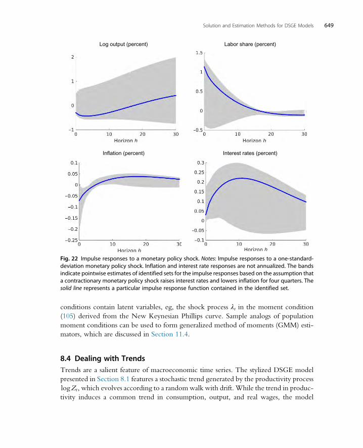
conditions contain latent variables, eg, the shock process λt in the moment condition

(105) derived from the New Keynesian Phillips curve. Sample analogs of population

moment conditions can be used to form generalized method of moments (GMM) esti-

mators, which are discussed in Section 11.4.

8.4 Dealing with TrendsTrends are a salient feature of macroeconomic time series. The stylized DSGE model

presented in Section 8.1 features a stochastic trend generated by the productivity process

logZt, which evolves according to a randomwalk with drift. While the trend in produc-

tivity induces a common trend in consumption, output, and real wages, the model

Log output (percent)

Inflation (percent)

Labor share (percent)

Interest rates (percent)

Fig. 22 Impulse responses to a monetary policy shock. Notes: Impulse responses to a one-standard-deviation monetary policy shock. Inflation and interest rate responses are not annualized. The bandsindicate pointwise estimates of identified sets for the impulse responses based on the assumption thata contractionary monetary policy shock raises interest rates and lowers inflation for four quarters. Thesolid line represents a particular impulse response function contained in the identified set.


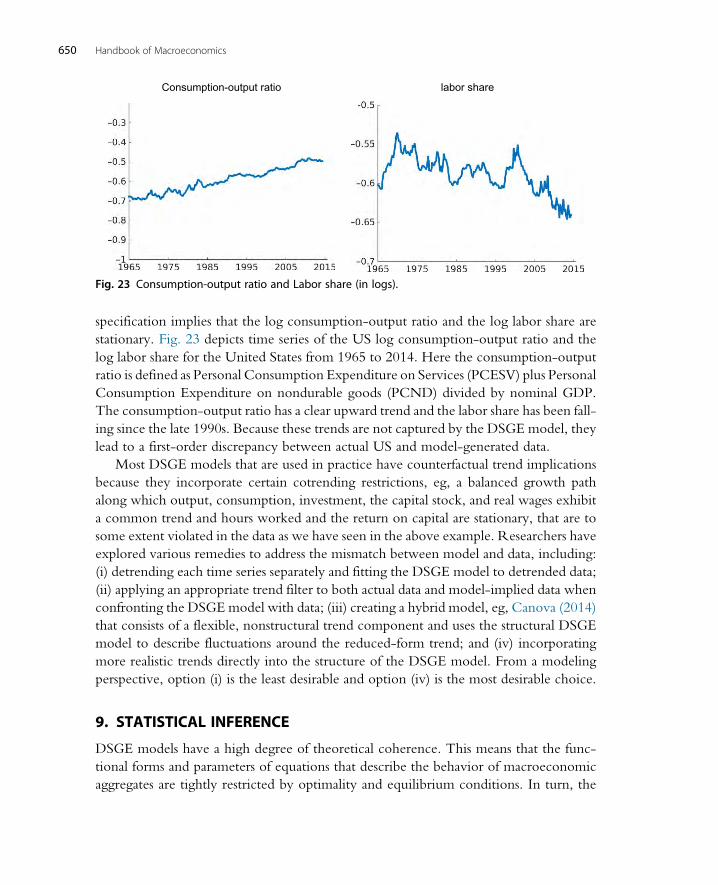
specification implies that the log consumption-output ratio and the log labor share are

stationary. Fig. 23 depicts time series of the US log consumption-output ratio and the

log labor share for the United States from 1965 to 2014. Here the consumption-output

ratio is defined as Personal Consumption Expenditure on Services (PCESV) plus Personal

Consumption Expenditure on nondurable goods (PCND) divided by nominal GDP.

The consumption-output ratio has a clear upward trend and the labor share has been fall-

ing since the late 1990s. Because these trends are not captured by the DSGE model, they

lead to a first-order discrepancy between actual US and model-generated data.

Most DSGE models that are used in practice have counterfactual trend implications

because they incorporate certain cotrending restrictions, eg, a balanced growth path

along which output, consumption, investment, the capital stock, and real wages exhibit

a common trend and hours worked and the return on capital are stationary, that are to

some extent violated in the data as we have seen in the above example. Researchers have

explored various remedies to address the mismatch between model and data, including:

(i) detrending each time series separately and fitting the DSGE model to detrended data;

(ii) applying an appropriate trend filter to both actual data and model-implied data when

confronting the DSGE model with data; (iii) creating a hybrid model, eg, Canova (2014)

that consists of a flexible, nonstructural trend component and uses the structural DSGE

model to describe fluctuations around the reduced-form trend; and (iv) incorporating

more realistic trends directly into the structure of the DSGE model. From a modeling

perspective, option (i) is the least desirable and option (iv) is the most desirable choice.

9. STATISTICAL INFERENCE

DSGE models have a high degree of theoretical coherence. This means that the func-

tional forms and parameters of equations that describe the behavior of macroeconomic

aggregates are tightly restricted by optimality and equilibrium conditions. In turn, the

Consumption-output ratio labor share

Fig. 23 Consumption-output ratio and Labor share (in logs).


family of probability distributions p(Y jθ), θ 2 Θ, generated by a DSGE model tends to

be more restrictive than the family of distributions associated with an atheoretical model,

such as a reduced-form VAR as in (113). This may place the empirical researcher in

a situation in which the data favor the atheoretical model and the atheoretical model

generates more accurate forecasts, but a theoretically coherent model is required for

the analysis of a particular economic policy. The subsequent discussion of statistical infer-

ence will devote special attention to this misspecification problem.

The goal of statistical inference is to infer an unknown parameter vector θ from obser-

vations Y; to provide a measure of uncertainty about θ; and to document the fit of the

statistical model. The implementation of these tasks becomes more complicated if

the statistical model suffers from misspecification. Confronting DSGE models with data

can essentially take two forms. If it is reasonable to assume that the probabilistic structure

of the DSGE model is well specified, then one can ask how far the observed data Yo1:T or

sample statistics SðYo1:T Þ computed from the observed data fall into the tails of the

model-implied distribution derived from p(Y1:Tjθ). The parameter vector θ can be

chosen to ensure that the density (likelihood) of SðYo1:TÞ is high under the distribution

p(Y1:Tjθ). If, on the other hand, there is a strong belief (possibly supported by empirical

evidence) that the probabilistic structure of the DSGE model is not rich enough to cap-

ture the salient features of the observed data, it is more sensible to consider a reference

model with a well-specified probabilistic structure, use it to estimate some of the pop-

ulation objects introduced in Section 8.2, and compare these estimates to their model

counterparts.

In Section 9.1 we ask the question whether the DSGE model parameters can be

determined based on observations Y and review the recent literature on identification.

We then proceed by reviewing two modes of statistical inference: frequentist and

Bayesian.ak We pay special attention to the consequences of model misspecification. Fre-

quentist inference, introduced in Section 9.2, takes a preexperimental perspective and

focuses on the behavior of estimators and test statistics, which are functions of the obser-

vations Y, in repeated sampling under the distribution Yθ . Frequentist inference is con-

ditioned on a “true” but unknown parameter θ, or on a data-generating process (DGP),

which is a hypothetical probability distribution under which the data are assumed to be

generated. Frequentist procedures have to be well behaved for all values of θ 2Θ. Bayes-ian inference, introduced in Section 9.3, takes a postexperimental perspective by treating

the unknown parameter θ as a random variable and updating a prior distribution p(θ) inview of the data Y using Bayes Theorem to obtain the posterior distribution p(θjY ).

Estimation and inference requires that the model be solved many times for different

parameter values θ. The subsequent numerical illustrations are based on the stylized

ak A comparison between econometric inference approaches and the calibration approach advocated by

Kydland and Prescott (1982) can be found in Rıos-Rull et al. (2012).


DSGE model introduced in Section 8.1, for which we have a closed-form solution.

However, such closed-form solutions are the exception and typically not available for

models used in serious empirical applications. Thus, estimationmethods, both frequentist

and Bayesian, have to be closely linked to model solution procedures. This ultimately

leads to a trade-off: given a fixed amount of computational resources, the more time

is spent on solving a model conditional on a particular θ, eg, through the use of a sophis-ticated projection technique, the less often an estimation objective function can be eval-

uated. For this reason, much of the empirical work relies on first-order perturbation

approximations of DSGE models, which can be obtained very quickly. The estimation

of models solved with numerically sophisticated projection methods is relatively rare,

because it requires a lot of computational resources. Moreover, as discussed in Part I, per-

turbation solutions are more easily applicable to models with a high-dimensional state

vector and such models, in turn, are less prone to misspecification and are therefore more

easily amenable to estimation. However, the recent emergence of low-cost parallel pro-

gramming environments and cloud computing will make it feasible for a broad group of

researchers to solve and estimate elaborate nonlinear DSGE models in the near future.

9.1 IdentificationThe question of whether a parameter vector θ is identifiable based on a sample Y is of

fundamental importance for statistical inference because one of the main objectives is

to infer the unknown θ based on the sample Y. Suppose that the DSGE model generates

a family of probability distributions p(Y jθ), θ 2Θ. Moreover, imagine a stylized setting in

which data are in fact generated from the DSGE model conditional on some “true”

parameter θ0. The parameter vector θ0 is globally identifiable if

pðY jθÞ¼ pðY jθ0Þ implies θ¼ θ0: (121)

The statement is somewhat delicate because it depends on the sample Y. From a preex-

perimental perspective, the sample is unobserved and it is required that (121) holds with

probability one under the distribution p(Y jθ0). From a postexperimental perspective, the

parameter θmay be identifiable for some trajectories Y, but not for others. The following

example highlights the subtle difference. Suppose that

y1, tjðθ,y2, tÞ� iidN θy2, t,1ð Þ, y2, t ¼ 0 w:p: 1=2� iidNð0,1Þ w:p: 1=2

�

Thus, with probability (w.p.) 1/2, one observes a trajectory along which θ is not iden-

tifiable because y2,t ¼ 0 for all t. If, on the other hand, y2,t 6¼ 0, then θ is identifiable.

9.1.1 Local IdentificationIf condition (121) is only satisfied for values of θ in an open neighborhood of θ0, then θ0 islocally identified. Most of the literature has focused on devising procedures to check local


identification in linearized DSGE models with Gaussian innovations. In this case the

distribution of Y jθ is a joint normal distribution and can be characterized by a Tny � 1

vector of means μ(θ) (where n is the dimension of the vector yt) and a Tny � Tnycovariance matrix Σ(θ). Defining m(θ) ¼ [μ(θ)0, vech(Σ(θ))0]0, where vech(�) vectorizesthe nonredundant elements of a symmetric matrix, we can restate the identification

condition as

mðθÞ¼mðθ0Þ implies θ¼ θ0: (122)

Thus, verifying the local identification condition is akin to checking whether the

Jacobian

J ðθÞ¼ @

@θ0mðθÞ (123)

is of full rank. This approach was proposed and applied by Iskrev (2010) to examine the

identification of linearizedDSGEmodels. If the joint distribution ofY is not Gaussian, say

because the DSGEmodel innovations Et are non-Gaussian or because the DSGEmodel is

nonlinear, then it is possible that θ0 is not identifiable based on the first and second

moments m(θ), but that there are other moments that make it possible to distinguish

θ0 from θ�6¼ θ0.

Local identification conditions are often stated in terms of the so-called information

matrix. Using Jensen’s inequality, it is straightforward to verify that the Kullback–Leibler

discrepancy between p(Y jθ0) and p(Y jθ) is nonnegative:

ΔKLðθjθ0Þ¼�Z

logpðY jθÞpðY jθ0Þ �

pðY jθ0ÞdY � 0: (124)

Under a nondegenerate probability distribution for Y, the relationship holds with equal-

ity only if p(Y jθ)¼ p(Y jθ0). Thus, we deduce that the Kullback–Leibler distance is min-

imized at θ ¼ θ0 and that θ0 is identified if θ0 is the unique minimizer of ΔKL(θjθ0). Let‘ðθjYÞ¼ logpðY jθÞ denote the log-likelihood function andr2

θ‘ðθjYÞ denote the matrix

of second derivatives of the log-likelihood function with respect to θ (Hessian), then

(under suitable regularity conditions that allow the exchange of integration and

differentiation)

rθ2ΔKLðθ0jθ0Þ¼Z

rθ2‘ðθ0jYÞpðY jθ0ÞdY : (125)

In turn, the model is locally identified at θ0 if the expected Hessian matrix is nonsingular.

For linearized Gaussian DSGE models that can be written in the form

Y �N μðθÞ,ΣðθÞð Þ we obtainZr2

θ‘ðθ0jYÞpðY jθ0ÞdY ¼J ðθÞ0ΩJ ðθÞ, (126)


where Ω is the Hessian matrix associated with the unrestricted parameter vector

m ¼ [μ0, vech(Σ)0]0 of a N(μ,Σ). Because Ω is a symmetric full-rank matrix of dimension

dim(m), we deduce that the Hessian is of full rank whenever the Jacobian matrix in (123)

is of full rank.

Qu and Tkachenko (2012) focus on the spectral density matrix of the process yt.

Using a frequency domain approximation of the likelihood function and utilizing the

information matrix equality, they express the Hessian as the outer product of the Jacobian

matrix of derivatives of the spectral density with respect to θ

Gðθ0Þ¼Z π

�π

@

@θ0vecðfyyðωÞ0Þ

�0 @

@θ0vecðfyyðωÞÞ

�dω (127)

and propose to verify whether G(θ0) is of full rank. The identification checks of Iskrev

(2010) and Qu and Tkachenko (2012) have to be implemented numerically. For each

conjectured θ0 the user has to compute the rank of the matrices J ðθ0Þ orG(θ0), respec-tively. Because in a typical implementation the computation of the matrices relies on

numerical differentiation (and integration), careful attention has be paid to the numerical

tolerance level of the procedure that computes the matrix rank. Detailed discussions can

be found in the two referenced papers.

Komunjer and Ng (2011) take a different route to assess the local identification of

linearized DSGE models. They examine the relationship between the coefficients of

the state-space representation of the DSGE model and the parameter vector θ. Recall

that the state-space representation takes the form

yt ¼Ψ0ðθÞ+Ψ1ðθÞ, st ¼Φ1ðθÞst�1 +ΦEðθÞEt: (128)

The notation highlights the dependence of the coefficient matrices on θ. Now stack the

coefficients of the Ψ and Φ matrices in the vector ϕ:

ϕ¼ vecðΨ0Þ0,vecðΨ1Þ0,vecðΦ1Þ0,vecðΦEÞ0� �0

:

It is tempting to conjecture that θ is locally identifiable if the Jacobian matrix associated

with the mapping from economic parameters θ to the reduced-form state-space param-

eters ϕ

@

@θ0ϕðθÞ (129)

has full column rank at θ0. The problem with this conjecture is that the reduced-form

parameters ϕ themselves are not identifiable. Let A be a nonsingular ns � ns matrix

and Ω an nE � nE orthogonal matrix, then we can define

s�t ¼Ast, Et

�¼ΩEt, Ψ�1¼Ψ1A

�1, Φ�1¼Φ1A

�1, Φ�E¼AΦEΩ0

to obtain an observationally equivalent state-space system


yt ¼Ψ0 +Ψ�1s�t, st ¼Φ

�1 s�t�1 +Φ

�EEt (130)

with ϕ 6¼ ϕ�. Thus, the number of identifiable reduced-form parameters is smaller than

the number of elements in theΨ andΦmatrices. The main contribution in Komunjer and

Ng (2011) is to account for the nonidentifiability of the reduced-form state-space param-

eters when formulating a rank condition along the lines of (129). In many DSGE models

a subset of the state transitions are deterministic, which complicates the formal analysis.

Identification becomes generally more tenuous the fewer variables are included in the

vector yt. For instance, in the context of the stylized DSGE model, suppose yt only

includes the labor share. According to (70) the law of motion for the labor share is

the sum of three AR(1) processes and an iid monetary policy shock. It can be rewritten

as an ARMA(3,3) process and therefore has at most 8 identifiable reduced-form param-

eters. Thus, the upper bound on the number of reduced-form parameters is less than the

number of DSGEmodel parameters, which is 13. In turn, it is not possible to identify the

entire θ vector.

9.1.2 Global IdentificationGlobal identification is more difficult to verify than local identification. Consider the

following example from Schorfheide (2013):

yt ¼ ½1 1�st, st ¼ θ21 0

1�θ21�θ1θ2 ð1�θ21Þ�

st�1 +1

0

� Et, Et � iidNð0,1Þ: (131)

Letting L denote the lag operator with the property that Lyt¼ yt�1, one can write the law

of motion of yt as an restricted ARMA(2,1) process:

1�θ21L� �

1�ð1�θ21ÞL� �

yt ¼ 1�θ1θ2Lð ÞEt: (132)

It can be verified that given θ1 and θ2, an observationally equivalent process can be

obtained by choosing θ�1 and θ

�2 such that

θ�1¼

ffiffiffiffiffiffiffiffiffiffiffiffi1�θ21

q, θ

�2¼ θ1θ2=θ

�1:

Here we switched the values of the two roots of the autoregressive lag polynomial. Qu

and Tkachenko (2014) propose to check for global identification by searching for solu-

tions to the equation

0¼△KLðθjθ0Þ, θ2Θ: (133)

If θ0 is the unique solution, then the DSGE model is globally identified. The authors

evaluate the Kullback–Leibler discrepancy using a frequency domain transformation.

The computational challenge is to find all the roots associated with (133). Kociecki

and Kolasa (2015) follow a slightly different approach that is attractive because it requires

the user to solve the DSGE model only at θ0, but not at all the other values of θ 2 Θ.


9.2 Frequentist InferenceThe fundamental problem of statistical inference is to infer the parameter vector θ, in ourcase the DSGE model parameters, based on a random sample Y. Frequentist inference

adopts a preexperimental perspective and examines the sampling distribution of estima-

tors and test statistics, which are transformations of the random sampleY, conditional on a

hypothetical DGP.We will distinguish between two cases. First, we consider the stylized

case in which the DSGE model is correctly specified. Formally, this means that Y is sam-

pled from p(Y jθ0), where the density p(Y jθ0) is derived from the DSGE model and θ isthe “true” but unknown parameter vector.al Second, we consider the case of misspeci-

fication, meaning the DSGE model is too stylized to capture some of the key features of

the data Y. As a consequence, the sampling distribution of Y has to be characterized by a

reference model, for instance, a VAR or a linear process. In terms of notation, we will

distinguish between the DSGE model, denoted byM1, and the reference modelM0. To

avoid confusion about which model generates the sampling distribution of Y, we add the

model indicator to the conditioning set and write, eg, p(Y jθ,M1) or p(Y jM0).We also use

the notation kakW ¼ a0Wa.

9.2.1 “Correct” Specification of DSGE ModelUnder the assumption of correct specification, the DSGE model itself is the DGP and

p(Y jθ0,M1) describes the sampling distribution of Y under which the behavior of

estimators and test statistics is being analyzed. In this case it is desirable to let the

model-implied probability distribution p(Y jθ0,M1) determine the choice of the objective

function for estimators and test statistics to obtain a statistical procedure that is efficient

(meaning that the estimator is close to θ0 with high probability in repeated sampling).

In this regard, the maximum likelihood (ML) estimator

θml ¼ argmaxθ2Θ logpðY jθ,M1Þ (134)

plays a central role in frequentist inference, because it is efficient under fairly general reg-

ularity conditions. One of these conditions is that θ0 is identifiable.Alternative estimators can be obtained by constructing an objective functionQT(θjY )

that measures the discrepancy between sample statistics mT ðYÞ (see Section 8.3) and

model-implied population statistics ½mTðYÞjθ,M1� (see Section 8.2). Examples of the

vector mT ðYÞ are, for instance, vectorized sample autocovariances such as

al In reality, of course, the observed Y is never generated from a probabilistic mechanism. Instead it reflects

measured macroeconomic activity. Thus, by “correct specification of a DSGE model” we mean that we

believe that its probabilistic structure is rich enough to assign high probability to the salient features of

macroeconomic time series.


mTðYÞ¼ vechðΓyyð0ÞÞ0,vecðΓyyð1ÞÞ0� �¼ 1

T

XTt¼1

mðyt�1:tÞ

or the OLS estimator of the coefficients of a VAR(1) (here without intercept)

mT ðYÞ¼ vec1

T

XTt¼1

yt�1y0t�1

!�11

T

XTt¼1

yt�1y0t

!:

We write the estimation objective function as

QT ðθjYÞ¼ mT ðYÞ�½mT ðYÞjθ,M1�k kWT, (135)

where WT is a symmetric positive-definite weight matrix. Under the assumption of a

correctly specified DSGE model, the optimal choice of the weight matrix WT is the

inverse of the DSGE model-implied covariance matrix of mTðYÞ. Thus, more weight

is assigned to sample moments that accurately approximate the underlying population

moment. The minimum distance (MD) estimator of θ is defined as

θmd ¼ argmaxθ2Θ QTðθjYÞ: (136)

Econometric inference is based on the sampling distribution of the estimator θmd and

confidence sets and test statistics derived from θmd and QT (θjY ) under the distribution

p(Y jθ0, M1).

9.2.2 Misspecification and Incompleteness of DSGE ModelsModel misspecification can be interpreted as a violation of the cross-coefficient restric-

tions embodied in the mapping from the DSGE model parameters θ into the system

matrices Ψ0, Ψ1, Φ1, and ΦE of the state-space representation in (76) and (78). An exam-

ple of an incomplete model is a version of the stylized DSGE model in which we do not

fully specify the law of motion for the exogenous shock processes and restrict our

attention to certain moment conditions, such as the consumption Euler equation. In

some cases, incompleteness and misspecification are two sides of the same coin. Consider

a version of the stylized DSGE model with only one structural shock, namely, the mon-

etary policy shock. This version does not contain sufficiently many shocks to explain the

observed variability in output growth, the labor share, inflation, and the interest rate.

More specifically, the one-shock DSGE model implies, for instance, that the linear

combination

1

κpð1+ νÞxER=β+ σRRt� 1

κpð1+ νÞxERπ t ¼ 0

is perfectly predictable; see (72) and (73). This prediction is clearly counterfactual. We

could regard the model as misspecified, in the sense that its predictions are at odds with


the data; or as incomplete, in the sense that adding more structural shocks could reduce

the gap between model and reality.

Regardless of whether the DSGE model is incomplete or misspecificed, it does not

produce a sampling distribution for the data Y that can be used to determine the frequen-

tist behavior of estimators and test statistics. In order to conduct a frequentist analysis, we

require a reference model M0 that determines the distribution of the data p(Y jM0) and

can be treated as a DGP. The reference model could be a fully specified parametric model

such as a VAR, p(Y jϕ, M0), where ϕ is a finite-dimensional parameter vector. Alterna-

tively, the reference model could be a general stochastic process for {yt} that satisfies a set

of regularity conditions necessary to establish large sample approximations of the sam-

pling distributions of estimators and test statistics.

If the DSGEmodel is incompletely specified, it is still possible to uphold the notion of

a “true” parameter vector θ0, in the sense that one could imagine the DGP to be the

incompletely specified DSGE model augmented by a set of equations (potentially with

additional parameters). If the DSGE model is misspecified, then the concept of a “true”

parameter value has to be replaced by the notion of a pseudo-true (or pseudo-optimal)

parameter value. The definition of a pseudo-true parameter value requires a notion of

discrepancy between the DGP p(Y jM0) and the DSGE model p(Y jθ, M1). Different

discrepancies lead to different pseudo-optimal values. Likelihood-based inference is asso-

ciated with the Kullback–Leibler discrepancy and would lead to

θ0ðKLÞ¼ argminθ2Θ �Z

logpðY jθ,M1ÞpðY jM0Þ

�pðY jM0ÞdY : (137)

Moment-based inference based on the sample objective function QT(θjY ) is associated

with a pseudo-optimal value

θ0ðQ,W Þ¼ argminθ2Θ QðθjM0Þ, (138)

where

QðθjM0Þ¼ ½mTðYÞjM0��½mðYÞjθ,M1�k kW :

Ultimately, the sampling properties of estimators and test statistics have to be derived

from the reference model M0.

9.3 Bayesian InferenceUnder the Bayesian paradigm, the calculus of probability is used not only to deal with

uncertainty about shocks Et, states st, and observations yt, but also to deal with uncertaintyabout the parameter vector θ. The initial state of knowledge (or ignorance) is summarized

by a prior distribution with density p(θ). This prior is combined with the conditional

distribution of the data given θ, ie, the likelihood function, to characterize the joint dis-

tribution of parameters and data. Bayes Theorem is applied to obtain the conditional


distribution of the parameters given the observed data Y. This distribution is called the

posterior distribution:

pðθjY ,M1Þ¼ pðY jθ,M1ÞpðθjM1ÞpðY jM1Þ , pðY jM1Þ¼

ZpðY jθ,M1ÞpðθjM1Þdθ: (139)

The posterior distribution contains all the information about θ conditional on sample

information Y. In a Bayesian setting a model comprises the likelihood function

p(Y jθ, M1) and the prior p(θjM1).

The posterior distribution of transformations of the DSGE model parameters θ, say,h(θ), eg, autocovariances and impulse response functions, can be derived from

p(θjY, M1). For instance,

YfhðθÞ� �hg¼Zθ j hðθÞ��h

pðθjY ,M1Þdθ: (140)

Solutions to inference problems can generally be obtained by specifying a suitable loss

function, stating the inference problem as a decision problem, and minimizing posterior

expected loss. For instance, to obtain a point estimator for h(θ), let L hðθÞ,δð Þ describe theloss associated with reporting δ if h(θ) is correct. The optimal decision δ* is obtained by

minimizing the posterior expected loss:

δ� ¼ argminδ2D

ZL hðθÞ,δð ÞpðθjY ,M1Þdθ: (141)

If the loss function is quadratic, then the optimal point estimator is the posterior mean

of h(θ).The most difficult aspect of Bayesian inference is the characterization of the posterior

moments of h(θ). Unfortunately, it is not possible to derive these moments analytically for

DSGE models. Thus, researchers have to rely on numerical methods. The Bayesian

literature has developed a sophisticated set of algorithms to generate draws θi from the pos-

terior distribution, such that averages of these draws converge to posterior expectations:

½hðθÞjY ,M1� ¼Z

hðθÞpðθjY ,M1Þdθ� 1

N

XNi¼1

hðθiÞ: (142)

Several of these computational techniques are discussed in more detail in Section 12.

9.3.1 “Correct” Specification of DSGE ModelsThe use of Bayes Theorem to learn about the DSGEmodel parameters implicitly assumes

that the researcher regards the probabilistic structure of the DSGEmodel as well specified

in the sense that there are parameters θ in the support of the prior distribution conditionalon which the salient features of the data Y are assigned a high probability. Of course, in

practice there is always concern that an alternative DSGE model may deliver a better


description of the data. The Bayesian framework is well suited to account for model

uncertainty.

Suppose the researcher contemplates two model specificationsM1 and M2, assuming

that one of them is correct. It is natural to place prior probabilities on the two models,

which we denote by πj,0. Ratios of model probabilities are called model odds. The pos-

terior odds of M1 vs M2 are given by

π1,Tπ2,T

¼ π1,0π2,0

pðY jM1ÞpðY jM2Þ , (143)

where the first factor on the right-hand side captures the prior odds and the second factor,

called Bayes factor, is the ratio of marginal data densities. Note that p(Y jMi) appears in the

denominator of Bayes Theorem (139). Posterior model odds and probabilities have

been widely used in the DSGE model literature to compare model specification or to

take averages across DSGE models. Prominent applications include Rabanal and

Rubio-Ramırez (2005) and Smets and Wouters (2007).

9.3.2 Misspecification of DSGE ModelsAs in the frequentist case, model misspecification complicates inference. Several

approaches have been developed in the literature to adapt Bayesian analysis to the poten-

tial misspecification of DSGEmodels. In general, the model space needs to be augmented

by a more densely parameterized reference model, M0, that provides a more realistic

probabilistic representation of the data.

Schorfheide (2000) considers a setting in which a researcher is interested in the rel-

ative ability of two (or more) DSGE models, say, M1 and M2, to explain certain popu-

lation characteristics φ, eg, autocovariances or impulse responses.am However, the DSGE

models may be potentially misspecified and the researcher considers a reference model

M0. As long as it is possible to form a posterior distribution for φ based on the reference

model, the overall posterior can be described by

pðφjYÞ¼X

j¼0,1,2πj,TpðφjY ,MjÞ: (144)

If one of the DSGE models is well specified, this model receives high posterior proba-

bility and dominates the mixture. If both DSGE models are at odds with the data, the

posterior probability of the reference model will be close to one. Given a loss function

over predictions of φ, one can compute DSGE model-specific predictions:

φðjÞ ¼ argminφ�

ZLðφ� ,φÞpðφjY ,MjÞdφ, j¼ 1,2: (145)

amFrequentist versions of this approach have been developed in Hnatkosvaka et al. (2012) and Marmer and

Otsu (2012).


Finally, the two DSGE models can be ranked based on the posterior riskZLðφðjÞ,φÞpðφjYÞdφ: (146)

Geweke (2010) assumes that the researcher regards the DSGEmodels not as models of the

data Y, but as models of some population moments φ. A reference modelM0, eg, a VAR,

provides the model for Y, but also permits the computation of implied population

moments. He shows that under these assumptions, one can define the posterior odds

of DSGE models as

π1,Tπ2,T

¼ π1,0π2,0

RpðφjM1ÞpðφjY ,M0ÞdφRpðφjM2ÞpðφjY ,M0Þdφ : (147)

Roughly, if we were able to observe φ, then p(φjMj) is the marginal likelihood. How-

ever, φ is unobservable and therefore replaced by a posterior predictive distribution

obtained from a reference model M0. The odds in favor of model M1 are high if there

is a lot of overlap between the preditive distribution for the population moments φ under

the DSGE model, and the posterior distribution of φ obtained when estimating the

reference model M0.

Building on work by Ingram and Whiteman (1994); Del Negro and Schorfheide

(2004) do not treat the DSGE model as a model of the data Y, but instead use it to con-

struct a prior distribution for a VAR. Consider the companion form VAR in (114). Use

the DSGE model to generate a prior distribution for ðΦ� 1,Φ�0, Σ

�Þ and combine this prior

with the VAR likelihood function

pðY ,Φ� 0,Φ�1,Σ

�,θjλÞ¼ pðY jΦ� 0

,Φ�1, Σ

�ÞpðΦ� 0,Φ�1, Σ

� jθ,λÞpðθÞ: (148)

The resulting hierarchical model is called a DSGE-VAR. The prior pðΦ� 0,Φ�1, Σ

� jθ,λÞ iscentered on restriction functions

Φ� �0ðθÞ, Φ

� �1ðθÞ, Σ

��ðθÞ,but allows for deviations from these restriction functions to account for model misspe-

cification. The parameter λ is a hyperparameter that controls the magnitude of the devi-

ations (prior variance) from the restriction function. This framework can be used for

forecasting, to assess the fit of DSGE models, eg, Del Negro et al. (2007), and to conduct

policy analysis, eg, Del Negro and Schorfheide (2009).

In a setting in which the reference model M0 plays a dominating role, Fernandez-

Villaverde and Rubio-Ramırez (2004) show that choosing the DSGE model that attains

the highest posterior probability (among, say, competing DSGEmodelsM1 andM2) leads

asymptotically to the specification that is closest to M0 in a Kullback–Leibler sense.

Rather than using posterior probabilities to select among or average across two DSGE

models, one can form a prediction pool, which is essentially a linear combination of

two predictive densities:


λpðytjY1:t�1,M1Þ+ ð1�λÞpðytjY1:t�1,M2Þ:The weight λ 2 [0,1] can be determined based on

YTt¼1

λpðytjY1:t�1,M1Þ+ ð1� λÞpðytjY1:t�1,M2Þ½ �:

This objective function could either be maximized with respect to λ or it can be treated asa likelihood function for λ and embedded in a Bayesian inference procedure. This idea is

developed in Geweke and Amisano (2011) and Geweke and Amisano (2012). Dynamic

versions with λ depending on time t are provided by Waggoner and Zha (2012) and

Del Negro et al. (2014).

10. THE LIKELIHOOD FUNCTION

The likelihood function plays a central role in both frequentist and Bayesian inference.

The likelihood function treats the joint density of the observables conditional on the

parameters, p(Y1:Tjθ), as a function of θ. The state-space representation of the DSGE

model leads to a joint distribution p(Y1:T,S1:Tjθ); see (79). In order to obtain the likeli-

hood function, one needs to integrate out the (hidden) states S1:T. This can be done

recursively, using an algorithm that is a called a filter.

This section focuses on the numerical evaluation of the likelihood function condi-

tional on a particular parameterization θ through the use of linear and nonlinear filters.

We assume that the DSGE model has the following, possibly nonlinear, state-space

representation:

yt ¼Ψðst, t;θÞ+ ut, ut �Fuð � ;θÞst ¼Φðst�1,Et;θÞ, Et �FEð � ;θÞ:

(149)

The state-space system is restricted in two dimensions. First, the errors in the measure-

ment equation enter in an additively separable manner. This implies that the conditional

density p(ytjst,θ) is given by pu yt�Ψðst, t;θÞjθð Þ, where pu(�jθ) is the pdf associated with

the measurement error distribution Fu(�;θ). In the absence of measurement errors, the

distribution ytj(st,θ) is a pointmass at Ψ(st,t;θ). Second, the state-transition equation

has a first-order Markov structure.an Owing to the first-order Markov structure of the

state-transition equation, neither the states st�2,st�3,… nor the observations

yt�1,yt�2,… provide any additional information about st conditional on st�1. Thus,

an Additional lags of the state vector could be easily incorporated using a companion form representation of

the state vector as in (114).


pðstjst�1,θÞ¼ pðstjst�1,S1:t�2,θÞ¼ pðstjst�1,S1:t�2,Y1:t�1,θÞ: (150)

For the linearized DSGE model of Section 8.1 with normally distributed measurement

errors ut � N(0,Σu) the conditional distributions are given by stjðst�1,θÞ�N Φ1st�1,ΦEΦ0

E

� �and ytj(st,θ) � N(Ψ0 +Ψ1st,Σu).

10.1 A Generic FilterWe now describe a generic filter that can be used to recursively compute the conditional

distributions p(stjY1:t,θ) and p(ytjY1:t�1,θ), starting from an initialization p(s0jθ). The dis-tributions p(stjY1:t,θ) are a by-product of the algorithm and summarize the information

about the state st conditional on the current and past observations Y1:t, which may be of

independent interest. The sequence of predictive distributions p(ytjY1:t�1,θ), t¼ 1,…,T,

can be used to obtain the likelihood function, which can be factorized as follows

pðY1:T jθÞ¼YTt¼1

pðytjY1:t�1,θÞ: (151)

The filter is summarized in Algorithm 5. In the description of the filter we drop the

parameter θ from the conditioning set to simplify the notation.

Algorithm 5 (Generic Filter). Let p(s0) ¼ p(s0jY1:0) be the initial distribution of the

state. For t ¼ 1 to T:

1. Forecasting t given t � 1:

(a) Transition equation:

pðstjY1:t�1Þ¼Z

pðstjst�1,Y1:t�1Þpðst�1jY1:t�1Þdst�1

(b) Measurement equation:

pðytjY1:t�1Þ¼Z

pðytjst,Y1:t�1ÞpðstjY1:t�1Þdst

2. Updating with Bayes Theorem. Once yt becomes available:

pðstjY1:tÞ¼ pðstjyt,Y1:t�1Þ¼ pðytjst,Y1:t�1ÞpðstjY1:t�1ÞpðytjY1:t�1Þ :

10.2 Likelihood Function for a Linearized DSGE ModelFor illustrative purposes, consider the prototypical DSGE model. Owing to the simple

structure of the model, we can use (69), (70), (72), and (73) to solve for the latent shocks

ϕt, λt, zt, and ER,t as a function of xt, ^lsht, π t, and Rt. Thus, we can deduce from (78) and

the definition of st that conditional on x0, the states st can be uniquely inferred from the

observables yt in a recursive manner, meaning that the conditional distributions


pðstjY1:t, x0Þ are degenerate. Thus, the only uncertainty about the state stems from the

initial condition.

Suppose that we drop the labor share and the interest rates from the definition of yt. In

this case it is no longer possible to uniquely determine st as a function of yt and x0, because

we only have two equations, (69) and (72), and four unknowns. The filter in Algorithm 5

now essentially solves an underdetermined system of equations, taking into account the

probability distribution of the four hidden processes. For our linearized DSGE model

with Gaussian innovations, all the distributions that appear in Algorithm 5 are Gaussian.

In this case the Kalman filter can be used to compute the means and covariance matrices

of these distributions recursively. To complete the model specification, we make the

following distributional assumptions about the initial state s0:

s0�N �s0j0,P0j0� �

:

In stationary models it is common to set �s0j0 and P0j0 equal to the unconditional first and

second moments of the invariant distribution associated with the law of motion of st in

(76). The four conditional distributions in the description of Algorithm 5 for a linear

Gaussian state-space model are summarized in Table 6. Detailed derivations can be found

in textbook treatments of the Kalman filter and smoother, eg, Hamilton (1994) or Durbin

and Koopman (2001).

To illustrate the Kalman filter algorithm, we simulate T ¼ 50 observations from the

stylized DSGE model conditional on the parameters in Table 5. The two left panels of

Fig. 24 depict the filtered shock processes ϕt and zt based on observations of only output

growth, which are defined as ½stjY1:t�. The bands delimit 90% credible intervals which

are centered around the filtered estimates and based on the standard deviationsffiffiffiffiffiffiffiffiffiffiffiffiffiffiffiffiffi½stjY1:t�

p. The information in the output growth series is not sufficient to generate

a precise estimate of the preference shock process ϕt, which, according to the forecast

Table 6 Conditional distributions for the Kalman filterDistribution Mean and variance

st�1jY1:t�1 N �st�1jt�1,Pt�1jt�1

� �Given from Iteration t � 1

stjY1:t�1 N �stjt�1,Ptjt�1

� ��stjt�1 ¼Φ1�st�1jt�1

Ptjt�1¼Φ1Pt�1jt�1Φ10 +ΦEΣEΦE

0

ytjY1:t�1 N �ytjt�1,Ftjt�1

� ��ytjt�1 ¼Ψ0 +Ψ1�stjt�1

Ftjt�1¼Ψ1Ptjt�1Ψ10 +Σu

stjY1:t N �stjt,Ptjt� �

�stjt ¼�stjt�1 + Ptjt�1Ψ01F

�1tjt�1ðyt��ytjt�1Þ

Ptjt ¼ Ptjt�1�Ptjt�1Ψ01F

�1tjt�1

Ψ1Ptjt�1

stj(St+1:T,Y1:T) N �stjt+1,Ptjt+1

� ��stjt+1 ¼�stjt + PtjtΦ0

1P�1t+1jtðst +1�Φ1�stjtÞ

Ptjt+1 ¼ Ptjt�PtjtΦ01P

�1t+1jtΦ1Ptjt


error variance decomposition in Fig. 17, only explains a small fraction of the variation in

output growth. The two right panels of Fig. 24 showwhat happens to the inference about

the hidden states if inflation and labor share are added to the set of observables.

Conditional on the three series, it is possible to obtain fairly sharp estimates of both

the preference shock ϕt and the technology growth shock zt.

Instead of using the Kalman filter, in a linearized DSGE model with Gaussian inno-

vations it is possible to characterize the joint distribution of the observables directly. Let Y

be a T � ny matrix composed of rows yt0. Then the joint distribution of Y is given by

vecðYÞjθ�N I Φ0ðθÞ,

Γyyð0jθÞ Γyyð1jθÞ … ΓyyðT �1jθÞΓ0yyð1jθÞ Γyyð0jθÞ … ΓyyðT �2jθÞ... ..

. . .. ..

.

Γ0yyðT �1jθÞ Γ0

yyðT �2jθÞ … Γyyð0jθÞ

26664

37775

0BBB@

1CCCA:

(152)

ft based on yt = log(Xt/Xt−1) ft based on yt = [log(Xt/Xt−1), lsht ,p t ]�

zt based on yt = log(Xt/Xt−1) zt based on yt = [log(Xt/Xt−1),lsht ,p t ]�

Fig. 24 Filtered states. Notes: The filtered states are based on a simulated sample of T ¼50 observations. Each panel shows the true state st (dotted), the filtered state ½stjY1:t� (dashed),and 90% credible bands based on p(stjY1:t) (grey area).


The evaluation of the likelihood function requires the calculation of the autocovariance

sequence and the inversion of an nyT � nyT matrix. For large T the joint density can be

approximated by the so-called Whittle likelihood function

pW ðY jθÞ∝YT�1

j¼0

2πf �1yy ðωjjθÞ

�� !1=2

exp �1

2

XT�1

j¼0

tr f �1yy ðωjjθÞf yyðωjÞh i( )

(153)

where fyy(ωjθ) is the DSGE model-implied spectral density, f yyðωÞ is the sample period-

ogram, and the ωj’s are the fundamental frequencies. The attractive feature of this like-

lihood function is that the researcher can introduce weights for the different frequencies,

and, for instance, only consider business cycle frequencies in the construction of the like-

lihood function. For the estimation of DSGE models, the Whittle likelihood has been

used, for instance, by Christiano and Vigfusson (2003), Qu and Tkachenko (2012),

and Sala (2015).

10.3 Likelihood Function for Nonlinear DSGE ModelsIf the DSGE model is solved using a nonlinear approximation technique, then either the

state-transition equation, or the measurement equation, or both become nonlinear. As

a consequence, analytical representations of the densities p(st�1jY1:t�1), p(stjY1:t�1),

and p(ytjY1:t�1) that appear in Algorithm 5 are no longer available. While there exists

a large literature on nonlinear filtering (see for instance Crisan and Rozovsky, 2011)

we focus on the class of particle filters. Particle filters belong to the class of sequential

Monte Carlo algorithms. The basic idea is to approximate the distribution stjY1:t through

a swarm of particles fsjt ,Wjt gMj¼1 such that

�ht,M ¼ 1

M

XMj¼1

hðsjtÞWjt �!a:s: ½hðstÞjY1:t�,

ffiffiffiffiffiM

p�ht,M �½hðstÞjY1:t�ð Þ ¼) N 0,Ωt½h�ð Þ,

(154)

where¼) denotes convergence in distribution.ao Here the sjt’s are particle values and the

Wjt ’s are the particle weights. The conditional expectation of h(st) is approximated by a

weighted average of the (transformed) particles hðsjtÞ. Under suitable regularity condi-

tions, the Monte Carlo approximation satisfies an SLLN and a CLT. The covariance

matrix Ωt[h] characterizes the accuracy of the Monte Carlo approximation. Setting

h(st) ¼ p(yt+1jst) yields the particle filter approximation of the likelihood increment

pðyt+1jY1:tÞ¼½pðyt+1jstÞjY1:t�. Each iteration of the filter manipulates the particle

values and weights to recursively track the sequence of conditional distributions stjY1:t.

The paper by Fernandez-Villaverde and Rubio-Ramırez (2007) was the first to

ao A sequence of random variables XT converges in distribution to a random variable X if for every measur-

able and bounded function f(�) that is continuous almost everywhere ½f ðXT Þ�!½f ðXÞ�.


approximate the likelihood function of a nonlinear DSGE model using a particle filter

and many authors have followed this approach.

Particle filters are widely used in engineering and statistics. Surveys and tutorials are

provided, for instance, in Arulampalam et al. (2002), Capp�e et al. (2007), Doucet and

Johansen (2011), and Creal (2012). The basic bootstrap particle filter algorithm is remark-

ably straightforward, but may perform quite poorly in practice. Thus, much of the

literature focuses on refinements of the bootstrap filter that increases the efficiency of

the algorithm; see, for instance, Doucet et al. (2001). Textbook treatments of the statis-

tical theory underlying particle filters can be found in Liu (2001), Capp�e et al. (2005), andDel Moral (2013).

10.3.1 Generic Particle FilterThe subsequent exposition draws from Herbst and Schorfheide (2015), who provide a

detailed presentation of particle filtering techniques in the context of DSGEmodel appli-

cations as well as a more extensive literature survey. In the basic version of the particle

filter, the time t particles are generated based on the time t� 1 particles by simulating the

state-transition equation forward. The particle weights are then updated based on the

likelihood of the observation yt under the sjt particle, pðytjsjtÞ. The more accurate the pre-

diction of yt based on sjt, the larger the density pðytjsjtÞ, and the larger the relative weight

that will be placed on particle j. However, the naive forward simulation ignores infor-

mation contained in the current observation yt andmay lead to a very uneven distribution

of particle weights, in particular, if the measurement error variance is small or if the model

has difficulties explaining the period t observation in the sense that for most particles sjt the

actual observation yt lies far in the tails of the model-implied distribution of ytjsjt. Theparticle filter can be generalized by allowing s

jt in the forecasting step to be drawn from

a generic importance sampling density gtð � jsjt�1Þ, which leads to the following

algorithm:ap

Algorithm 6 (Generic Particle Filter).

1. Initialization. Draw the initial particles from the distribution sj0�iidp(s0) and set

W0j ¼ 1, j ¼ 1,…,M.

2. Recursion. For t ¼ 1,…,T:

(a) Forecasting st. Draw s�j

t from density gt( s�tjst�1

j ) and define the importance

weights

ωjt ¼ pð s�j

tjsjt�1Þgtð s�j

t jsjt�1Þ : (155)

An approximation of E[h(st)jY1:t�1] is given by

ap To simplify the notation, we omit θ from the conditioning set.


ht,M ¼ 1

M

XMj¼1

hð s� jtÞωj

tWjt�1: (156)

(b) Forecasting yt. Define the incremental weights

w� j

t¼ pðytj s�j

tÞωjt: (157)

The predictive density p(ytjY1:t�1) can be approximated by

pðytjY1:t�1Þ¼ 1

M

XMj¼1

w� j

tWjt�1: (158)

(c) Updating. Define the normalized weights

W� j

t ¼w� j

tWjt�1

1

M

XM

j¼1w� j

tWjt�1

: (159)

An approximation of [h(st)jY1:t,θ] is given by

h�t,M

¼ 1

M

XMj¼1

hð s�j

tÞW� j

t: (160)

(d) Selection. Resample the particles via multinomial resampling. Let {stj}j¼1M

denoteM iid draws from a multinomial distribution characterized by support points

and weights f s�j

t,W� j

tg and setWtj ¼ 1 for j ¼,1…,M. An approximation of [h(st)j

Y1:t,θ] is given by

�ht,M ¼ 1

M

XMj¼1

hðs jt ÞWjt : (161)

3. Likelihood Approximation. The approximation of the log likelihood function is

given by

log pðY1:T jθÞ¼XTt¼1

log1

M

XMj¼1

w� j

tWjt�1

!: (162)

Conditional on the stage t � 1 weights Wjt�1 the accuracy of the approximation of the

likelihood increment p(ytjY1:t�1) depends on the variability of the incremental weightsω� j

t

in (157). The larger the variance of the incremental weights, the less accurate the particle

filter approximation of the likelihood function. In this regard, the most important choice

for the implementation of the particle filter is the choice of the proposal distribution

gtð s�j

tjsjt�1Þ, which is discussed in more detail below.


The selection step is included in the filter to avoid a degeneracy of particle weights.

While it adds additional noise to the Monte Carlo approximation, it simultaneously

equalizes the particle weights, which increases the accuracy of subsequent approxima-

tions. In the absence of the selection step, the distribution of particle weights would

become more uneven from iteration to iteration. The selection step does not have to

be executed in every iteration. For instance, in practice, users often apply a threshold rule

according to which the selection step is executed whenever the following measure falls

below a threshold, eg, 25% or 50% of the nominal number of particles:

dESSt ¼M=1

M

XMj¼1

ðW� jtÞ2

!: (163)

The effective sample size dESSt (in terms of number of particles) captures the variance of

the particle weights. It is equal toM ifW� j

t ¼ 1 for all j and equal to 1 if one of the particles

has weightM and all others have weight 0. The resampling can be executed with a variety

of algorithms. We mention multinomial resampling in the description of Algorithm 6.

Multinomial resampling is easy to implement and satisfies a CLT. However, there are

more efficient algorithms (meaning they are associated with a smaller Monte Carlo var-

iance), such as stratified or systematic resampling. A detailed textbook treatment can be

found in Liu (2001) and Capp�e et al. (2005).

10.3.2 Bootstrap Particle FilterThe bootstrap particle filter draws s

�jt from the state-transition equation and sets

gtð s� jtjsjt�1Þ¼ pð s�j

tjsjt�1Þ: (164)

This implies that ωjt ¼ 1 and the incremental weight is given by the likelihood pðytj s�j

tÞ,which unfortunately may be highly variable. Fig. 25 provides an illustration of the boot-

strap particle filter with M ¼ 100 particles using the same experimental design as for the

Kalman filter in Section 10.2. The observables are output growth, labor share, and infla-

tion and the observation equation is augmented with measurement errors. The measure-

ment error variance amounts to 10% of the total variance of the simulated data. Because

the stylized DSGE is loglinearized, the Kalman filter provides exact inference and any

discrepancy between the Kalman and particle filter output reflects the approximation

error of the particle filter. In this application the particle filter approximations are quite

accurate even with a small number of particles. The particle filtered states zt and ER,tappear to be more volatile than the exactly filtered states from the Kalman filter.

Fig. 26 illustrates the accuracy of the likelihood approximation. The left panel com-

pares log-likelihood increments logpðytjY1:t�1,θÞ obtained from the Kalman filter and a

single run of the particle filter. The left panel shows the distribution of the approximation

errors of the log-likelihood function: log pðY1:T jθÞ� logpðY1:T jθÞ. It has been shown,


eg, by Del Moral (2004) and Pitt et al. (2012), that the particle filter approximation of the

likelihood function is unbiased, which implies that the approximation of the log-likeli-

hood function has a downward bias, which is evident in the figure. Under suitable reg-

ularity conditions the particle filter approximations satisfy a CLT. The figure clearly

indicates that the distribution of the approximation errors becomes more concentrated

as the number of particles is increased from M ¼ 100 to M ¼ 500.

The accuracy of the bootstrap particle filter crucially depends on the quality of the fit

of the DSGE model and the magnitude of the variance of the measurement errors ut.

Recall that for the bootstrap particle filter, the incremental weights w� jt ¼ pðytj s�j

tÞ. Ifthe model fits poorly, then the one-step-ahead predictions conditional on the particles

s�j

t are inaccurate and the density of the actual observation yt falls far in the tails of the

predictive distribution. Because the density tends to decay quickly in the tails, the

ft λt

zt εR,t

Fig. 25 Particle-filtered states. Notes: We simulate a sample of T¼ 50 observations yt and states st fromthe stylized DSGE model. The four panels compare filtered states from the Kalman filter (solid) and asingle run of the particle filter (dashed) with M ¼ 100 particles. The observables used for filtering areoutput growth, labor share, and inflation. The measurement error variances are 10% of the totalvariance of the data.


incremental weights will have a high variability, which means that Monte Carlo approx-

imations based on these incremental weights will be inaccurate.

The measurement error defines a metric between the observation yt and the condi-

tional mean prediction Ψ(st,t;θ). Consider the extreme case in which the measurement

error is set to zero. This means that any particle that does not predict yt exactly would get

weight zero. In a model in which the error distribution is continuous, the probability of

drawing a s�jt that receives a nonzero weight is zero, which means that the algorithm

would fail in the first iteration. By continuity, the smaller the measurement error vari-

ance, the smaller the number of particles that would receive a nontrivial weight, and the

larger the variance of the approximation error of particle filter approximations. In prac-

tice, it is often useful to start the filtering with a rather large measurement error variance,

eg, 10% or 20% of the variance of the observables, and then observing the accuracy of the

filter as the measurement error variance is reduced.

10.3.3 (Approximately) Conditionally Optimal Particle FilterThe conditionally optimal particle filter sets

gtð s�t jsjt�1Þ¼ pð s�tjyt, sjt�1Þ, (165)

that is, s�t is sampled from the posterior distribution of the period t state given ðyt, sjt�1Þ.

In this case

w� j

t¼Z

pðytjstÞpðstjsjt�1Þdst ¼ pðytjsjt�1Þ: (166)

Log-likelihood approximation Distribution of approx. errors

Fig. 26 Particle-filtered log-likelihood. Notes: We simulate a sample of T¼ 50 observations yt and statesst from the stylized DSGE model. The left panel compares log-likelihood increments from the Kalmanfilter (solid) and a single run of the particle filter (dashed) withM¼ 100 particles. The right panel shows adensity plot for approximation errors of log pðY1:T jyÞ� logpðY1:T jyÞ based on Nrun¼ 100 repetitions ofthe particle filter for M ¼ 100 (solid), M ¼ 200 (dotted), and M ¼ 500 (dashed) particles. Themeasurement error variances are 10% of the total variance of the data.


Unfortunately, in a typical nonlinear DSGEmodel applications it is not possible to sample

directly from pð s�tjyt, sjt�1Þ. In this case the researcher could try to approximate the con-

ditionally optimal proposal density, which leads to an approximately conditionally optimal

particle filter. For instance, if the DSGE model’s nonlinearity arises from a higher-order

perturbation solution and the nonlinearities are not too strong, then an approximately

conditionally optimal importance distribution could be obtained by applying the one-

step Kalman filter updating described in Table 6 to the first-order approximation of

the DSGE model. More generally, as suggested in Guo et al. (2005), one could use

the updating steps of a conventional nonlinear filter, such as an extended Kalman filter,

unscented Kalman filter, or a Gaussian quadrature filter, to construct an efficient proposal

distribution. Approximate filters for nonlinear DSGE models have been developed by

Andreasen (2013) and Kollmann (2015).

Whenever one uses a proposal distribution that differs from pð s�jtjsjt�1Þ it becomes nec-

essary to evaluate the density pð s�jtjsjt�1Þ. In DSGE model applications, one typically does

not have a closed-form representation for this density. It is implicitly determined by the

distribution of Et and the state transitionΦ(st�1,Et). The problem of having to evaluate the

DSGE model-implied density of s�jt can be avoided by sampling an innovation from a

proposal density gEðE�tjsjt�1Þ and defining s�jt ¼Φðsjt�1, E

�tÞ. In this case the particle weights

can be updated by the density ratio

ωjt ¼ pEðE�j

tÞgtðE�

j

tjsjt�1Þ

, (167)

where pE(�) is the model-implied pdf of the innovation Et.Sometimes, DSGE models have a specific structure that may simplify the particle-

filter-based likelihood approximation. In models that are linear conditional on a subset

of state variables, eg, volatility states or Markov-switching regimes, it is possible to use

the Kalman filter to represent the uncertainty about a subset of states. In models in which

the number of shocks Et equals the number of observables yt, it might be possible (in the

absence of measurement errors) conditional on an initial state vector s0 to directly solve for

Et based on yt and st�1, which means that it may be possible to evaluate the likelihood

function p(Y1:Tjθ,s0) recursively. A more detailed discussion of these and other issues

related to particle filtering for DSGEmodels is provided inHerbst and Schorfheide (2015).

11. FREQUENTIST ESTIMATION TECHNIQUES

We will now consider four frequentist inference techniques in more detail: likelihood-

based estimation (Section 11.1), simulated method of moments estimation

(Section 11.2), impulse response function matching (Section 11.3), and GMMestimation

(Section 11.4). All of these econometric techniques, with the exception of the impulse


response function matching approach, are widely used in other areas of economics and

are associated with extensive literatures that we will not do justice to in this section. We

will sketch the main idea behind each of the econometric procedures and then focus on

adjustments that have been proposed to tailor the techniques to DSGE model applica-

tions. Each estimation method is associated with a model evaluation procedure that

essentially assesses the extent to which the estimation objective has been achieved.

11.1 Likelihood-Based EstimationUnder the assumption that the econometric model is well specified, likelihood-based

inference techniques enjoy many optimality properties. Because DSGE models deliver

a joint distribution for the observables, maximum likelihood estimation of θ is very

appealing. The maximum likelihood estimator θml was defined in (134). Altug (1989)

andMcGrattan (1994) are early examples of papers that estimated variants of a neoclassical

stochastic growth model by maximum likelihood, whereas Leeper and Sims (1995)

estimated a DSGE model meant to be usable for monetary policy analysis.

Even in a loglinearized DSGE model, the DSGE model parameters θ enter the coef-ficients of the state-space representation in a nonlinear manner, which can be seen in

Table 4. Thus, a numerical technique is required to maximize the likelihood function.

A textbook treatment of numerical optimization routines can be found, for instance, in

Judd (1998) and Nocedal and Wright (2006). Some algorithms, eg, Quasi-Newton

methods, rely on the evaluation of the gradient of the objective function (which requires

differentiability), and other methods, such as simulated annealing, do not. This distinc-

tion is important if the likelihood function is evaluated with a particle filter. Without

further adjustments, particle filter approximations of the likelihood function are nondif-

ferentiable in θ even if the exact likelihood function is. This issue and possible solutions

are discussed, for instance, in Malik and Pitt (2011) and Kantas et al. (2014).

11.1.1 Textbook Analysis of the ML EstimatorUnder the assumption that θ is well identified and the log-likelihood function is suffi-

ciently smooth with respect to θ, confidence intervals and test statistics for the DSGE

model parameters can be based on a large sample approximation of the sampling

distribution of the ML estimator. A formal analysis in the context of state-space models

is provided, for instance, in the textbook by Capp�e et al. (2005).We sketch the main steps

of the approximation, assuming that the DSGE model is correctly specified and the data

are generated by p(Y jθ0,M1). Of course, this analysis could be generalized to a setting in

which the DSGE model is misspecified and the data are generated by a reference model

p(Y jM0). In this case the resulting estimator is called quasi-maximum-likelihood estima-

tor and the formula for the asymptotic covariance matrix presented below would

have to be adjusted. A detailed treatment of quasi-likelihood inference is provided in

White (1994).


Recall fromSection 10 that the log-likelihood function can be decomposed as follows:

‘T ðθjYÞ¼XTt¼1

logpðytjY1:t�1,θÞ¼XTt¼1

log

Zpðytjst,θÞpðstjY1:t�1Þdst: (168)

Owing to the time-dependent conditioning information Y1:t�1 the summands are not

stationary. However, under the assumption that the sequence {st,yt} is stationary if

initialized in the infinite past, one can approximate the log-likelihood function by

‘sT ðθjYÞ¼XTt¼1

log

Zpðytjst,θÞpðstjY�∞:t�1Þdst, (169)

and show that the discrepancy ‘TðθjYÞ� ‘sT ðθjYÞ�� becomes negligible as T !∞. The

ML estimator is consistent if T�1‘sT ðθjYÞ�!a:s: ‘sðθÞ uniformly almost surely (a.s.), where

‘s(θ) is deterministic and maximized at the “true” θ0. The consistency can be stated as

θml �!a:s: θ0: (170)

Frequentist asymptotics rely on a second-order approximation of the log-likelihood

function. Define the score (vector of first derivatives) rθ‘sTðθjYÞ and the matrix of

second derivatives (Hessian, multiplied by minus one) �r2θ‘

sT ðθjYÞ and let

‘sT ðθjYÞ¼ ‘sT ðθ0jYÞ+T�1=2rθ‘sTðθ0jYÞ

ffiffiffiffiT

pðθ�θ0Þ

+1

2

ffiffiffiffiT

pðθ�θ0Þ0 r2

θ‘sT ðθ0jYÞ

� � ffiffiffiffiT

pðθ�θ0Þ+ small:

If the maximum is attained in the interior of the parameter space Θ, the first-order con-ditions can be approximated byffiffiffiffi

Tp ðθml�θ0Þ¼ �r2

θ‘sT ðθ0jYÞ

� ��1T�1=2rθ‘

sTðθ0jYÞ+ small: (171)

Under suitable regularity conditions, the score process satisfies a CLT:

T�1=2rθ‘T ðθjYÞ¼)Nð0,Iðθ0ÞÞ, (172)

where Iðθ0Þ is the Fisher information matrix.aq As long as the likelihood function is cor-

rectly specified, the term k�r2θ‘T ðθjYÞ�Iðθ0Þ k converges to zero uniformly in a

neighborhood around θ0, which is a manifestation of the so-called information matrix

equality. This leads to the following resultffiffiffiffiT

p ðθml�θ0Þ¼)N 0,I�1ðθ0Þ� �

: (173)

aq The formal definition of the information matrix for this model is delicate and therefore omitted.


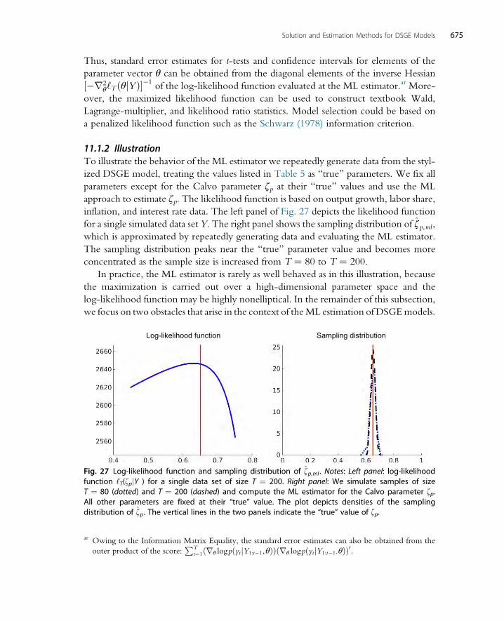
Thus, standard error estimates for t-tests and confidence intervals for elements of the

parameter vector θ can be obtained from the diagonal elements of the inverse Hessian

½�r2θ‘T ðθjYÞ��1

of the log-likelihood function evaluated at the ML estimator.ar More-

over, the maximized likelihood function can be used to construct textbook Wald,

Lagrange-multiplier, and likelihood ratio statistics. Model selection could be based on

a penalized likelihood function such as the Schwarz (1978) information criterion.

11.1.2 IllustrationTo illustrate the behavior of the ML estimator we repeatedly generate data from the styl-

ized DSGE model, treating the values listed in Table 5 as “true” parameters. We fix all

parameters except for the Calvo parameter ζp at their “true” values and use the ML

approach to estimate ζp. The likelihood function is based on output growth, labor share,

inflation, and interest rate data. The left panel of Fig. 27 depicts the likelihood function

for a single simulated data set Y. The right panel shows the sampling distribution of ζp,ml,which is approximated by repeatedly generating data and evaluating the ML estimator.

The sampling distribution peaks near the “true” parameter value and becomes more

concentrated as the sample size is increased from T ¼ 80 to T ¼ 200.

In practice, the ML estimator is rarely as well behaved as in this illustration, because

the maximization is carried out over a high-dimensional parameter space and the

log-likelihood function may be highly nonelliptical. In the remainder of this subsection,

we focus on two obstacles that arise in the context of theML estimation of DSGEmodels.

Log-likelihood function Sampling distribution

Fig. 27 Log-likelihood function and sampling distribution of zp,ml . Notes: Left panel: log-likelihoodfunction ‘T(zpjY ) for a single data set of size T ¼ 200. Right panel: We simulate samples of sizeT ¼ 80 (dotted) and T ¼ 200 (dashed) and compute the ML estimator for the Calvo parameter zp.All other parameters are fixed at their “true” value. The plot depicts densities of the samplingdistribution of zp . The vertical lines in the two panels indicate the “true” value of zp.

ar Owing to the Information Matrix Equality, the standard error estimates can also be obtained from the

outer product of the score:PT

t¼1 rθ logpðytjY1:t�1,θÞð Þ rθ logpðytjY1:t�1,θÞð Þ0.


The first obstacle is the potential stochastic singularity of the DSGE model-implied

conditional distribution of yt given its past. The second obstacle is caused by a potential

lack of identification of the DSGE model parameters.

11.1.3 Stochastic SingularityImagine removing all shocks except for the technology shock from the stylized DSGE

model, while maintaining that yt comprises output growth, the labor share, inflation,

and the interest rate. In this case, we have one exogenous shock and four observables,

which implies, among other things, that the DSGE model places probability one on

the event that

β logRt� logπt ¼ β logðπ*γ=βÞ� logπ*:

Because in the actual data β logRt� logπt is time varying, the likelihood function is equal

to zero and not usable for inference. The literature has adopted two types of approaches

to address the singularity, which we refer to as the “measurement error” approach and the

“more structural shocks” approach.

Under the measurement error approach (78) is augmented by a measurement error

process ut, which in general may be serially correlated. The term “measurement error” is

a bit of a misnomer. It tries to blame the discrepancy between the model and the data on

the accuracy of the latter rather than the quality of the former. In a typical DSGE model

application, the blame should probably be shared by both. A key feature of the

“measurement error” approach is that the agents in the model do not account for the

presence of utwhenmaking their decisions. The “measurement error” approach has been

particularly popular in the real business cycle literature—it was used, for instance, in

Altug (1989). The real business cycle literature tried to explain business cycle fluctuations

based on a small number of structural shocks, in particular, technology shocks.

The “more structural shocks” approach augments the DSGE model with additional

structural shocks until the number of shocks is equal to or exceeds the desired number of

observables stacked in the vector yt. For instance, if we add the three remaining shock

processes ϕt, λt, ER,t back into the prototypical DSGE model, then a stochastic singularity

is no longer an obstacle for the evaluation of the likelihood function. Of course, at a dee-

per level, the stochastic singularity problem never vanishes, as we could also increase the

dimension of the vector yt. Because the policy functions in the solution of the DSGE

model express the control variables as functions of the state variables, the set of potential

observables yt in any DSGE model exceeds the number of shocks (which are exogenous

state variables from the perspective of the underlying agents’ optimization problems).

Most of the literature that estimates loglinearized DSGE models uses empirical specifi-

cations in which the number of exogenous shocks is at least as large as the number of

observables. Examples are Schorfheide (2000), Rabanal and Rubio-Ramırez (2005),

and Smets and Wouters (2007).


The converse of the “more structural shocks” approach would be a “fewer

observables” approach, ie, one restricts the number of observables used in the construc-

tion of the likelihood function to the number of exogenous shocks included in the

model. This raises the question of which observables to include in the likelihood func-

tion, which is discussed in Guerron-Quintana (2010) and Canova et al. (2014). Qu

(2015) proposes to use a composite likelihood to estimate singular DSGE models.

A composite likelihood function is obtained by partitioning the vector of observables

yt into subsets, eg, yt0 ¼ [y1,t

0 ,y2,t0 ,y3,t0 ] for which the likelihood function is nonsingular,

eg, “composite likelihood” and then use the product of marginals p(Y1,1:Tjθ)p(Y2,1:Tjθ)p(Y3,1:Tjθ) as the estimation objective function.

11.1.4 Dealing with Lack of IdentificationIn many applications it is quite difficult to maximize the likelihood function. This dif-

ficulty is in part caused by the presence of local extrema and/or weak curvature in some

directions of the parameter space and may be a manifestation of identification problems.

One potential remedy that has been widely used in practice is to fix a subset of the param-

eters at plausible values, where “plausible” means consistent with some empirical obser-

vations that are not part of the estimation sample Y. Conditional on the fixed parameters,

the likelihood function for the remaining parameters may have a more elliptical shape and

therefore may be easier to maximize. Of course, such an approach ignores the uncertainty

with respect to those parameters that are being fixed. Moreover, if they are fixed at the

“wrong” parameter values, inference about the remaining parameters will be distorted.

Building on the broader literature on identification-robust econometric inference,

the recent literature has developed inference methods that remain valid even if some

parameters of the DSGE model are only weakly or not at all identified. Guerron-

Quintana et al. (2013) propose a method that relies on likelihood-based estimates of

the system matrices of the state-space representation Ψ0, Ψ1, Φ1 and ΦE. In view of

the identification problems associated with the Ψ and Φ matrices discussed in

Section 9.1, their approach requires a reparameterization of the state-space matrices in

terms of an identifiable reduced-form parameter vector ϕ ¼ f(θ) that, according to

the DSGE model, is a function of θ. In the context of our stylized DSGE model, such

a reparameterization could be obtained based on the information in Table 4.

LetMϕ1 denote the state-space representation of the DSGEmodel in terms ofϕ and let

ϕ be theML estimator ofϕ. The hypothesisH0 : θ¼ θ0 can be translated into the hypoth-esis ϕ ¼ f(θ0) and the corresponding likelihood ratio statistic takes the form

LRðY jθ0Þ¼ 2 logpðY jϕ,Mϕ1 Þ� logpðY jf ðθ0Þ,Mϕ

1 Þh i

¼)χ2dimðϕÞ: (174)

The degrees of freedom of the χ2 limit distribution depend on the dimension ofϕ (instead

of θ), which means that it is important to reduce the dimension of ϕ as much as possible

by using a minimal state-variable representation of the DSGE model solution and


to remove elements from the Ψ and Φ matrices that are zero for all values of θ.The likelihood ratio statistic can be inverted to generate a 1 � α joint confidence set

for the vector θ:

CSθðYÞ¼ θ j LRðY jθÞ� χ2crit�

, (175)

where χ2crit is the 1 � α quantile of the χ2dimðϕÞ distribution. Subvector inference can be

implemented by projecting the joint confidence set on the desired subspace. The inver-

sion of test statistics is computationally tedious because the test statistic has to be evaluated

for a wide range of θ values. However, it does not require the maximization of the like-

lihood function. Guerron-Quintana et al. (2013) show how the computation of the con-

fidence interval can be implemented based on the output from a Bayesian estimation of

the DSGE model.

Andrews andMikusheva (2015) propose an identification-robust Lagrange multiplier

test. The test statistic is based on the score process and its quadratic variation

sT , tðθÞ¼rθ‘ðθjY1:tÞ�rθ‘ðθjY1:t�1Þ, JT ðθÞ¼XTt¼1

sT , tðθÞs0T , tðθÞ

and is defined as

LMðθjYÞ¼r0θ‘T ðθ0jYÞ½ JTðθ0Þ��1rθ‘T ðθ0jYÞ¼)χ2dimðθ0Þ: (176)

Note that the degrees of freedom of the χ2 limit distribution now depend on the dimen-

sion of the parameter vector θ instead of the vector of identifiable reduced-form coef-

ficients. A confidence set for θ can be obtained by replacing the LR statistic in (175)

with the LM statistic. Andrews and Mikusheva (2015) also consider subvector inference

based on a profile likelihood function that concentrates out a subvector of well-identified

DSGE model parameters. A frequency domain version of the LM test based on the

Whittle likelihood function is provided by Qu (2014). Both Andrews and Mikusheva

(2015) and Qu (2014) provide detailed Monte Carlo studies to assess the performance

of the proposed identification-robust tests.

11.2 (Simulated) Minimum Distance EstimationMinimum distance (MD) estimation is based on the idea of minimizing the discrepancy

between sample moments of the data, which we denoted by mTðYÞ, and model-implied

moments, which we denoted by ½mT ðYÞjθ,M1�. The MD estimator θmd was defined in(135) and (136). Examples of the sample statistics mTðYÞ are the sample autocovariances

ΓyyðhÞ, a smoothed periodogram �f yyðωÞ as in Diebold et al. (1998), or estimates of the

parameters of an approximating model, eg, the VAR(p) in (113) as in Smith (1993). If

mTðYÞ consists of parameter estimates of a reference model, then the moment-based esti-

mation is also called indirect inference; see Gourieroux et al. (1993). In some cases it is


possible to calculate the model-implied moments analytically. For instance, suppose that

mT ðYÞ¼ 1

T

Xyty

0t�1, then we can derive

½mTðYÞjθ,M1� ¼ 1

T

X½yty0t�1jθ,M1� ¼½y2y01jθ,M1� (177)

from the state-space representation of a linearized DSGE model. Explict formulae for

moments of pruned models solved with perturbation methods are provided by

Andreasen et al. (2013) (recall Section 4.4). Alternatively, suppose that mTðYÞ corre-sponds to the OLS estimates of a VAR(1). In this case, even for a linear DSGE model,

it is not feasible to compute

½mT ðYÞ� ¼1

T

XTt¼1

yt�1y0t�1

!�11

T

XTt¼1

yt�1y0t

��θ,M1

" #: (178)

The model-implied expectation of the OLS estimator has to be approximated, for

instance, by a population regression:

½mTðYÞ� ¼ ½yt�1y0t�1jθ,M1�

� ��1½yt�1y

0tjθ,M1�, (179)

or the model-implied moment function has to be replaced by a simulation approxima-

tion, which will be discussed in more detail below.

11.2.1 Textbook AnalysisWe proceed by sketching the asymptotic approximation of the frequentist sampling

distribution of the MD estimator. Define the discrepancy

GT ðθjYÞ¼ mTðYÞ� ½mT ðYÞjθ,M1�, (180)

such that the criterion function of the MD estimator in (135) can be written as

QTðθjYÞ¼ GTðθjYÞk kWT: (181)

Suppose that there is a unique θ0 with the property thatas

mTðYÞ�½mT ðYÞjθ0,M1��!a:s: 0 (182)

and that the sample criterion function QT(θjY ) converges uniformly almost surely to a

limit criterion function Q(θ), then the MD estimator is consistent in the sense that

θmd!a:s: θ0.The analysis of the MD estimator closely mirrors the analysis of the ML estimator,

because both types of estimators are defined as the extremum of an objective function.

as In some DSGE models a subset of the series included in yt is nonstationary. Thus, moments are only well

defined after a stationarity-inducing transformation has been applied. This problem is analyzed in

Gorodnichenko and Ng (2010).


The sampling distribution of θmd can be derived from a second-order approximation of

the criterion function QT(θjY ) around θ0:

TQTðθjYÞ¼ffiffiffiffiT

prθQT ðθ0jYÞ

ffiffiffiffiT

pðθ�θ0Þ0

+1

2

ffiffiffiffiT

pðθ�θ0Þ0 1

Tr2

θQT ðθ0jYÞ� ffiffiffiffi

Tp

ðθ�θ0Þ+ small:(183)

If the minimum of QT(θjY ) is obtained in the interior, then

ffiffiffiffiT

p ðθmd�θ0Þ¼ � 1

Tr2

θQTðθ0jYÞ� �1 ffiffiffiffi

Tp rθQTðθ0jYÞ+ small: (184)

Using (180), the “score” process can be expressed asffiffiffiffiT

p rθQTðθ0jYÞ¼ rθGT ðθ0jYÞð ÞWT

ffiffiffiffiT

pGT ðθ0jYÞ (185)

and its distribution depends on the distribution offfiffiffiffiT

pGT ðθ0jYÞ¼

ffiffiffiffiT

pmTðYÞ�½mT ðYÞjθ0,M1�ð Þ

+ffiffiffiffiT

p½mT ðYÞjθ0,M1��½mTðYÞjθ0,M1��

¼ I + II ,

(186)

say. Term I captures the variability of the deviations of the sample moment mTðYÞ fromits expected value ½mT ðYÞjθ0,M1� and term II captures the error due to approximating

½mTðYÞjθ0,M1� by ½mT ðYÞjθ0,M1�. Under suitable regularity conditionsffiffiffiffiT

pGTðθ0jYÞ¼)N 0,Ωð Þ, (187)

and ffiffiffiffiT

p ðθmd�θ0Þ¼)N 0,ðDWD0Þ�1DWΩWD0ðDWD0Þ�1

� �, (188)

whereW is the limit of the sequence of weight matricesWT and thematrixD is defined as

the probability limit ofrθGT(θ0jY ). To construct tests and confidence sets based on the

limit distribution, the matrices D and Ω have to be replaced by consistent estimates. We

will discuss the structure of Ω in more detail below.

If the number of moment conditions exceeds the number of parameters, then the

model specification can be tested based on the overidentifying moment conditions. If

WT ¼ ½ΩT ��1, where ΩT is a consistent estimator of Ω, then

TQTðθmdjYÞ¼)χ2df , (189)

where the degrees of freedom df equal the number of overidentifying moment condi-

tions. The sample objective function can also be used to construct hypothesis tests for θ.Suppose that the null hypothesis is θ ¼ θ0. A quasi-likelihood ratio test is based on

TðQT ðθ0jYÞ�QT ðθmdjYÞ; a quasi-Lagrange-multiplier test is based on a properly


standardized quadratic form offfiffiffiffiT

p rθQT ðθ0jYÞ; and a Wald test is based on a properly

standardized quadratic form offfiffiffiffiT

p ðθmd�θ0Þ. Any of these test statistics can be inverted

to construct a confidence set. Moreover, if the parameters suffer from identification prob-

lems, then the approach of Andrews and Mikusheva (2015) can be used to conduct

identification-robust inference based on the quasi-Lagrange-multiplier test.

11.2.2 Approximating Model-Implied MomentsIn many instances the model-implied moments ½mTðYÞjθ,M1� are approximated by an

estimate ½mT ðYÞjθ,M1�. This approximation affects the distribution of θmd through

term II in (186). Consider the earlier example in (178) and (179) in which mT ðYÞ cor-responds to the OLS estimates of a VAR(1). Because the OLS estimator has a bias that

vanishes at rate 1/T, we can deduce that term II converges to zero and does not affect the

asymptotic covariance matrix Ω.Themore interesting case is theone inwhich ½mT ðYÞjθ,M1� is basedon the simulation

of the DSGEmodel. The asymptotic theory for simulation-based extremum estimators has

been developed in Pakes and Pollard (1989). Lee and Ingram (1991) and Smith Jr. (1993) are

the first papers that use simulated method of moments to estimate DSGE models. For

concreteness, suppose that mT(Y ) corresponds to the first-order (uncentered) sample auto-

covariances.We previously showed that, provided the yt’s are stationary,½mT ðYÞjθ,M1� isgiven by the DSGE model population autocovariance matrix ½y2y01jθ,M1�, which can beapproximated by simulating a sample of length λT of artificial observations Y * from the

DSGEmodelM1 conditional on θ. Based on these simulated observations one can compute

the sample autocovariances mλTðY �ðθ,M1ÞÞ. In this case term II is given by

II ¼ 1ffiffiffiλ

p ffiffiffiffiffiffiλT

p 1

λT

XλTt¼1

y�t y�t�1�½y2y01jθ0,M1�

!(190)

and satisfies a CLT. Because the simulated data are independent of the actual data, terms I

and II in (186) are independent and we can write

Ω¼∞½I �+∞½II �, (191)

where

∞½II � ¼ 1

λlimT!∞

T mT ðY �ðθ0,M1ÞÞ½ � �

(192)

and can be derived from the DSGEmodel. The larger λ, the more accurate the simulation

approximation and the contribution of ∞½II � to the overall covariance matrix Ω.We generated the simulation approximation by simulating one long sample of obser-

vations from the DSGE model. Alternatively, we could have simulated λ samples Y i,

i ¼ 1, λ of size T. It turns out that for the approximation, say, of ½y2y01jθ,M1�, it doesnot matter because mT ðY �ðθ,M1ÞÞ is an unbiased estimator of½y2y01jθ,M1�. However, if


mTðYÞ is defined as the OLS estimator of a VAR(1), then the small-sample bias of the

OLS estimator generates an O(T�1) wedge between

XλTt¼1

y�t�1y�0t�1

!�1XλTt¼1

y�t�1y�0t�1 and

XTt¼1

yt�1y0t�1

!�1XTt¼1

yt�1y0t�1

��θ,M1

" #:

For large values of λ, this wedge can be reduced by using

E½mT ðYÞjθ,M1� ¼ 1

λ

Xλi¼1

XTt¼1

yit�1yi0t�1

!�1XTt¼1

yit�1yi0t�1

instead. Averaging OLS estimators from model-generated data reproduces the O(T�1)

bias of the OLS estimator captured by ½mT ðYÞjθ0,M1� and can lead to a final sample

bias reduction in term II, which improves the small sample performance of θmd.at

When implementing the simulation approximation of the moments, it is important

to fix the random seed when generating the sample Y * such that for each parameter

value of θ the same sequence of random variables is used in computing Y *(θ,M1).

This ensures that the sample objective function QT(θjY ) remains sufficiently smooth

with respect to θ to render the second-order approximation of the objective function

valid.

11.2.3 MisspecificationUnder the assumption that the DSGE model is correctly specified, the MD estimator has

a well-defined almost-sure limit θ0 and the asymptotic variance∞½I � of term I in (186) is

given by the model-implied variance

∞½I � ¼ limT!∞

T mT ðY �ðθ0,M1ÞÞ½ � �

, (193)

which up to the factor of 1/λ is identical to the contribution ∞½II � of the simulation

approximation of the moments to the overall asymptotic variance Ω; see (192). Under

the assumption of correct specification, it is optimal to choose the weight matrixW based

on the accuracy with which the elements of the moment vector mTðYÞmeasure the pop-

ulation analog ½mTðYÞjθ0,M1�. If the number of moment conditions exceeds the num-

ber of parameters, it is optimal (in the sense of minimizing the sampling variance of θmd)to place more weight on matching moments that are accurately measured in the data,

by setting W ¼Ω�1. In finite sample, one can construct WT from a consistent estimator

of Ω�1.

at See Gourieroux et al. (2010) for a formal analysis in the context of a dynamic panel data model.


If the DSGE model is regarded as misspecified, then the sampling distribution of the

MD estimator has to be derived under the distribution of a reference model p(Y jM0).

In this case we can define

θ0ðQÞ¼ limT!∞

argminθ k½mTðYÞjM0��½mjθ,M1�jW (194)

and, under suitable regularity, the estimator θmd will converge to the pseudo-optimal

value θ0. Note that θ0 is a function of the moments mT ðYÞ that are being matched

and the weight matrix W (indicated by the Q argument). Both m and W are chosen

by the researcher based on the particular application. The vector m should correspond

to a set of moments that are deemed to be informative about the desired parameter-

ization of the DSGE model and reflect the ultimate purpose of the estimated DSGE

model. The weight matrix W should reflect beliefs about the informativeness of

certain sample moments with respect to the desired parameterization of the DSGE

model.

To provide an example, consider the case of a DSGEmodel with stochastic singularity

that attributes all business cycle fluctuations to technology shocks. To the extent that the

observed data are not consistent with this singularity, the model is misspecified.

A moment-based estimation of the model will ultimately lead to inflated estimates of

the standard deviation of the technology shock innovation, because this shock alone

has to generate the observed variability in, say, output growth, the labor share, and other

variables. The extent to which the estimated shock variance is upwardly biased depends

on exactly which moments the estimator is trying to match. If one of the priorities of the

estimation exercise is to match the unconditional variance of output growth, then the

weight matrix W should assign a large weight to this moment, even if it is imprecisely

measured by its sample analog in the data.

The asymptotic variance ∞½I � of term I in (186) is now determined by the variance

of the sample moments implied by the reference model M0:

∞½I � ¼ limT!∞

T½mTðYÞjM0� �

: (195)

Suppose that mT ðYÞ¼ 1

T

XT

t¼1yty

0t�1, which under suitable regularity conditions con-

verges to the population autocovariance matrix ½y1y00jM0� under the reference model

M0. If the reference model is a linear process, then the asymptotic theory developed

in Phillips and Solo (1992) can be used to determine the limit covariance matrix

∞½I �. An estimate of ∞½I � can be obtained with a heteroskedasticity and autocorrela-

tion consistent (HAC) covariance matrix estimator that accounts for the serial correlation

in the matrix-valued sequence fyty0t�1gTt¼1. An extension of indirect inference in which

mT ðYÞ comprises estimates of an approximating model to the case of misspecified DSGE

models is provided in Dridi et al. (2007).


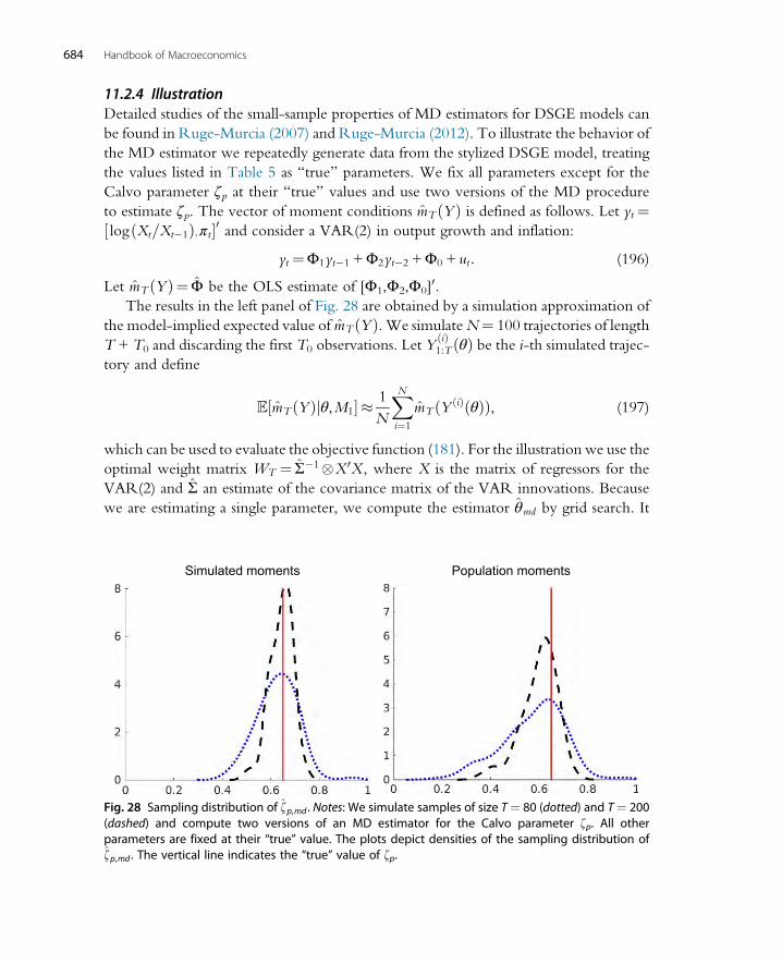
11.2.4 IllustrationDetailed studies of the small-sample properties of MD estimators for DSGE models can

be found in Ruge-Murcia (2007) and Ruge-Murcia (2012). To illustrate the behavior of

the MD estimator we repeatedly generate data from the stylized DSGE model, treating

the values listed in Table 5 as “true” parameters. We fix all parameters except for the

Calvo parameter ζp at their “true” values and use two versions of the MD procedure

to estimate ζp. The vector of moment conditions mT ðYÞ is defined as follows. Let yt ¼½ logðXt=Xt�1Þ,πt�0 and consider a VAR(2) in output growth and inflation:

yt ¼Φ1yt�1 +Φ2yt�2 +Φ0 + ut: (196)

Let mT ðYÞ¼ Φ be the OLS estimate of [Φ1,Φ2,Φ0]0.

The results in the left panel of Fig. 28 are obtained by a simulation approximation of

the model-implied expected value of mT ðYÞ. We simulateN¼ 100 trajectories of length

T + T0 and discarding the first T0 observations. Let YðiÞ1:T ðθÞ be the i-th simulated trajec-

tory and define

½mT ðYÞjθ,M1� � 1

N

XNi¼1

mT ðY ðiÞðθÞÞ, (197)

which can be used to evaluate the objective function (181). For the illustration we use the

optimal weight matrix WT ¼ Σ�1 X 0X , where X is the matrix of regressors for the

VAR(2) and Σ an estimate of the covariance matrix of the VAR innovations. Because

we are estimating a single parameter, we compute the estimator θmd by grid search. It

Simulated moments Population moments

Fig. 28 Sampling distribution of zp,md . Notes: We simulate samples of size T¼ 80 (dotted) and T¼ 200(dashed) and compute two versions of an MD estimator for the Calvo parameter zp. All otherparameters are fixed at their “true” value. The plots depict densities of the sampling distribution ofzp,md . The vertical line indicates the “true” value of zp.


is important to use the same sequence of random numbers for each value of θ2T to

compute the simulation approximation ½mT ðYÞjθ,M1�. The results in the right panel

of Fig. 28 are based on the VAR(2) approximation of the DSGE model based on a pop-

ulation regression. Let xt0 ¼ [yt�1

0,yt�20,1] and let

½mT ðYÞjθ,M1� � ½xtx0tjθ,M1�Þ� ��1½xty0tjθ,M1�: (198)

Fig. 28 depicts density estimates of the sampling distribution of ζp,md. The vertical lineindicates the “true” parameter value of ζp. As the sample size increases from T ¼ 80 to

T ¼ 200, the sampling distribution concentrates around the “true” value and starts to

look more like a normal distribution, as the asymptotic theory presented in this section

suggests. The distribution of the estimator based on the simulated objective function is

more symmetric around the “true” value and also less variable. However, even based on a

sample size of 200 observations, there is considerable uncertainty about the Calvo param-

eter and hence the slope of the NewKeynesian Phillips curve. A comparison with Fig. 27

indicates that the MD estimator considered in this illustration is less efficient than the ML

estimator.

11.2.5 Laplace Type EstimatorsIn DSGE model applications the estimation objective functionQT(θjY ) is often difficult

to optimize. Chernozhukov and Hong (2003) proposed computing a mean of a quasi-

posterior density instead of computing an extremum estimator. The resulting estimator is

called a Laplace-type (LT) estimator and defined as follows (provided the integral in the

denominator is well defined):

θLT ¼exp �1

2QT ðθjYÞ

� �Rexp �1

2QTðθjYÞ

� �dθ

: (199)

This estimator can be evaluated using the Metropolis–Hastings algorithm discussed in

Section 12.2 or the sequential Monte Carlo algorithm presented in Section 12.3 below.

The posterior computations may be more accurate than the computation of an extre-

mum. Moreover, suppose that the objective function is multimodal. In repeated sam-

pling, the extremum of the objective function may shift from one mode to the other,

making the estimator appear to be unstable. On the other hand, owing to the averaging,

the LT estimator may be more stable. Chernozhukov and Hong (2003) establish the

consistency and asymptotic normality of LT estimators, which is not surprising because

the sample objective function concentrates around its extremum as T !∞ and the dis-

crepancy between the extremum and the quasi-posterior mean vanishes. DSGE model

applications of LT estimators are provided in Kormilitsina and Nekipelov (2012, 2016).


LT estimators can be constructed not only fromMD estimators but also from IRFmatch-

ing estimators and GMM estimators discussed below.

11.3 Impulse Response Function MatchingAs discussed previously, sometimes DSGE models are misspecified because researchers

have deliberately omitted structural shocks that contribute to business cycle fluctuations.

An example of such a model is the one developed by Christiano et al. (2005). The authors

focus their analysis on the propagation of a single shock, namely, a monetary policy

shock. If it is clear that if the DSGE model does not contain enough structural shocks

to explain the variability in the observed data, then it is sensible to try to purge the effects

of the unspecified shocks from the data, before matching the DSGE model to the obser-

vations. This can be done by “filtering” the data through the lens of a VAR that identifies

the impulse responses to those shocks that are included in the DSGE model. The model

parameters can then be estimated byminimizing the discrepancy betweenmodel-implied

and empirical impulse response functions. A mismatch between the two sets of impulse

responses provides valuable information about the misspecification of the propagation

mechanism and can be used to develop better-fitting DSGE models. Influential papers

that estimate DSGE models by matching impulse response functions include

Rotemberg and Woodford (1997), Christiano et al. (2005), and Altig et al. (2011).

The casual description suggests that impulse response function matching estimators are

a special case of the previously discussed MD estimators (the DSGE modelM1 is misspe-

cified and a structural VAR serves as reference modelM0 under which the sampling dis-

tribution of the estimator is derived). Unfortunately, several complications arise, which

we will discuss in the remainder of this section. Throughout, we assume that the DSGE

model has been linearized. An extension to the case of nonlinear DSGE models is

discussed in Ruge-Murcia (2014).

11.3.1 Invertibility and Finite-Order VAR ApproximationsThe empirical impulse responses are based on a finite-order VAR, such as the one in (113).

However, even linearizedDSGEmodels typically cannot bewritten as a finite-order VAR.

Instead, they take the form of a state-space model, which typically has a VARMA repre-

sentation. In general we can distinguish the following three cases: (i) the solution of the

DSGE model can be expressed as a VAR(p). For the stylized DSGE model, this is the case

if yt is composed of four observables: output growth, the labor share, inflation, and interest

rates. (ii) The moving average polynomial of the VARMA representation of the DSGE

model is invertible. In this case the DSGE model can be expressed as an infinite-order

VAR driven by the structural shock innovations Et. (iii) The moving average polynomial

of the VARMA representation of the DSGE model is not invertible. In this case the inno-

vation of the VAR(∞) approximation do not correspond to the structural innovations Et.Only in case (i) can one expect a direct match between the empirical IRFs and the DSGE


model IRFs. Cases (ii) and (iii) complicate econometric inference. The extent to which

impulse-response-function-based estimation and model evaluation may be misleading

has been fiercely debated in Christiano et al. (2007) and Chari et al. (2008).

Fernandez-Villaverde et al. (2007) provide formal criteria to determine whether a

DSGE model falls under case (i), (ii), or (iii). Rather than presenting a general analysis

of this problem, we focus on a simple example. Consider the following twoMA processes

that represent the DSGE models in this example:

M1 : yt ¼ Et + θEt�1¼ð1+ θLÞEtM2 : yt ¼ θEt + Et�1¼ðθ+LÞEt, (200)

where 0 < θ < 1, L denotes the lag operator, and Et � iidN(0,1). ModelsM1 andM2 are

observationally equivalent, because they are associated with the same autocovariance

sequence. The root of the MA polynomial of model M1 is outside of the unit circle,

which implies that the MA polynomial is invertible and one can express yt as an

AR(∞) process:

ARð∞Þ for M1 : yt ¼�X∞j¼1

ð�θÞjyt�j + Et: (201)

It is straightforward to verify that the AR(∞) approximation reproduces the impulse

response function of M1:

@yt@Et

¼ 1,@yt+1

@Et¼ θ,

@yt+ h

@Et¼ 0 for h> 1:

Thus, the estimation of an autoregressive model with many lags can reproduce the

monotone impulse response function of model M1.

The root of the MA polynomial ofM2 lies inside the unit circle. WhileM2 could also

be expressed as an AR(∞), it would be a representation in terms of a serially uncorrelated

one-step-ahead forecast error ut that is a function of the infinite history of the Et’s: ut ¼(1+θL)�1(θ + L). As a consequence, the AR(∞) is unable to reproduce the hump-shaped

IRF of modelM2. More generally, if the DSGE model is associated with a noninvertible

moving average polynomial, its impulse responses cannot be approximated by a

VARð∞Þ and a direct comparison of VAR and DSGE IRFs may be misleading.

11.3.2 Practical ConsiderationsThe objective function for the IRF matching estimator takes the same form as the

criterion function of the method of moments estimator in (180) and (181), where

mT ðYÞ is the VAR IRF. For ½mT ðYÞjθ,M1� researchers typically just use the

DSGE model impulse response, say, IRF(�jθ,M1). In view of the problems caused by

noninvertible moving-average polynomials and finite-order VAR approximations of

infinite-order VAR representations, a more prudent approach would be to replace


IRF(�jθ,M1) by average impulse response functions that are obtained by repeatedly sim-

ulating data from the DSGE model (given θ) and estimating a structural VAR, as in the

indirect inference approach described in Section 11.2. Such a modification would address

the concerns about IRF matching estimators raised by Chari et al. (2008).

The sampling distribution of the IRF matching estimator depends on the sampling

distribution of the empirical VAR impulse responses mT ðYÞ under the VAR M0. An

approximation of the distribution of mTðYÞ could be obtained by first-order asymptotics

and the delta method as in L€utkepohl (1990) and Mittnik and Zadrozny (1993) for sta-

tionary VARs; or as in Phillips (1998), Rossi and Pesavento (2006), and Pesavento and

Rossi (2007) for VARs with persistent components. Alternatively, one could use the

bootstrap approximation proposed by Kilian (1998, 1999). If the number of impulse

responses stacked in the vector mTðYÞ exceeds the number of reduced-form VAR coef-

ficient estimates, then the sampling distribution of the IRFs becomes asymptotically sin-

gular. Guerron-Quintana et al. (2014) use nonstandard asymptotics to derive the

distribution of IRFs for the case in which there are more responses than reduced-form

parameters.

Because for high-dimensional vectors mT ðYÞ the joint covariance matrix may be

close to singular, researchers typically choose a diagonal weight matrix WT, where the

diagonal elements correspond to the inverse of the sampling variance for the estimated

response of variable i to shock j at horizon h. As discussed in Section 11.2, to the extent

that the DSGE model is misspecified, the choice of weight matrix affects the probability

limit of the IRF matching estimator and should reflect the researcher’s loss function.

In fact, impulse response function matching is appealing only if the researcher is con-

cerned about model misspecification. This misspecification might take two forms: First,

the propagation mechanism of the DSGEmodel is potentially misspecified and the goal is

to find pseudo-optimal parameter values that minimize the discrepancy between empir-

ical and model-implied impulse responses. Second, the propagation mechanisms for the

shocks of interest are believed to be correctly specified, but the model lacks sufficiently

many stochastic shocks to capture the observed variation in the data. In the second case, it

is in principle possible to recover the subset of “true” DSGE model parameters θ0 thataffect the propagation of the structural shock for which the IRF is computed. The con-

sistent estimation would require that the DSGE model allow for a VAR(∞) representa-

tion in terms of the structural shock innovations Et; that the number of lags included in

the empirical VAR increase with sample size T; and that the VAR identification scheme

correctly identify the shock of interest if the data are generated from a version of the

DSGE model that is augmented by additional structural shocks.

11.3.3 IllustrationTo illustrate the properties of the IRF matching estimator, we simulate data from the

stylized DSGE model using the parameter values given in Table 5. We assume that


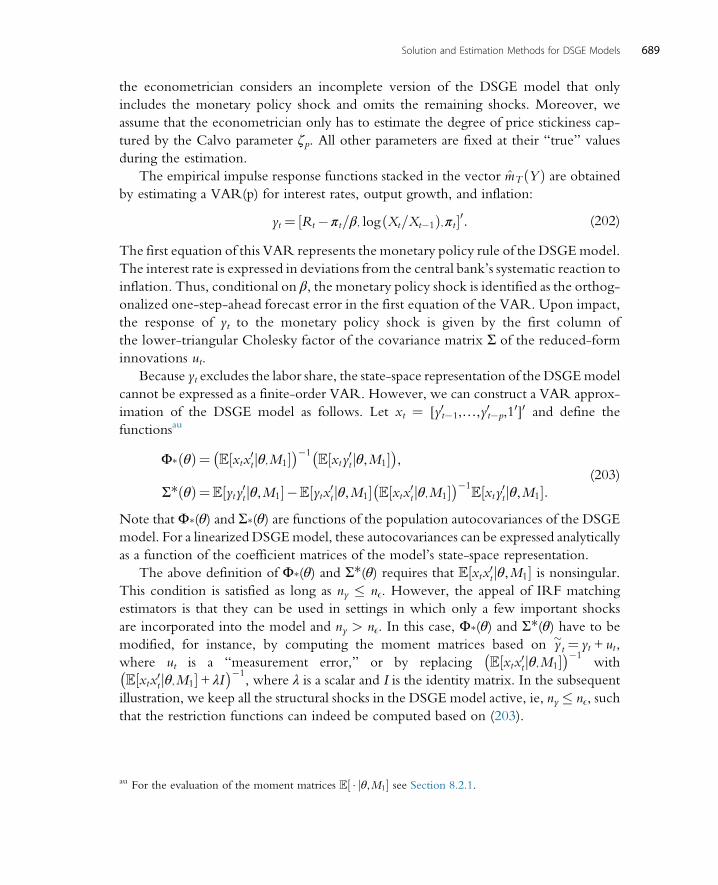
the econometrician considers an incomplete version of the DSGE model that only

includes the monetary policy shock and omits the remaining shocks. Moreover, we

assume that the econometrician only has to estimate the degree of price stickiness cap-

tured by the Calvo parameter ζp. All other parameters are fixed at their “true” values

during the estimation.

The empirical impulse response functions stacked in the vector mT ðYÞ are obtainedby estimating a VAR(p) for interest rates, output growth, and inflation:

yt ¼ Rt�πt=β, logðXt=Xt�1Þ,πt½ �0: (202)

The first equation of this VAR represents the monetary policy rule of the DSGEmodel.

The interest rate is expressed in deviations from the central bank’s systematic reaction to

inflation. Thus, conditional on β, the monetary policy shock is identified as the orthog-

onalized one-step-ahead forecast error in the first equation of the VAR. Upon impact,

the response of yt to the monetary policy shock is given by the first column of

the lower-triangular Cholesky factor of the covariance matrix Σ of the reduced-form

innovations ut.

Because yt excludes the labor share, the state-space representation of the DSGEmodel

cannot be expressed as a finite-order VAR. However, we can construct a VAR approx-

imation of the DSGE model as follows. Let xt ¼ [y0t�1,…,y0t�p,10]0 and define the

functionsau

Φ*ðθÞ¼ ½xtx0tjθ,M1�� 1

½xty0tjθ,M1��

,

Σ*ðθÞ¼½yty0tjθ,M1��½ytx0tjθ,M1� ½xtx0tjθ,M1�� 1

½xty0tjθ,M1�:(203)

Note that Φ*(θ) and Σ*(θ) are functions of the population autocovariances of the DSGE

model. For a linearized DSGEmodel, these autocovariances can be expressed analytically

as a function of the coefficient matrices of the model’s state-space representation.

The above definition of Φ*(θ) and Σ*(θ) requires that ½xtx0tjθ,M1� is nonsingular.This condition is satisfied as long as ny � nE. However, the appeal of IRF matching

estimators is that they can be used in settings in which only a few important shocks

are incorporated into the model and ny > nE. In this case, Φ*(θ) and Σ*(θ) have to be

modified, for instance, by computing the moment matrices based on y�t ¼ yt + ut,

where ut is a “measurement error,” or by replacing ½xtx0tjθ,M1�� 1

with

½xtx0tjθ,M1�+ λI� ��1

, where λ is a scalar and I is the identity matrix. In the subsequent

illustration, we keep all the structural shocks in the DSGE model active, ie, ny � nE, such

that the restriction functions can indeed be computed based on (203).

au For the evaluation of the moment matrices ½ � jθ,M1� see Section 8.2.1.


Fig. 29 compares the impulse responses from the state-space representation and the

VAR approximation of the DSGE model. It turns out that there is a substantial dis-

crepancy. Because the monetary policy shock is iid and the stylized DSGE model does

not have an endogenous propagation mechanism, both output and inflation revert

back to the steady state after one period. The VAR response, on the other hand, is

more persistent and the relative movement of output and inflation is distorted.

Augmenting a VAR(1) with additional lags has no noticeable effect on the impulse

response.

The IRF matching estimator minimizes the discrepancy between the empirical

and the DSGE model-implied impulse responses by varying ζp. Fig. 30 illustrates

the effect of ζp on the response of output and inflation. The larger ζp, the stronger

the nominal rigidity, and the larger the effect of a monetary policy shock on output.

Fig. 31 shows the sampling distribution of the IRF matching estimator for the sample

sizes T ¼ 80 and T ¼ 200. We match IRFs over 10 horizons and use an identity

weight matrix. If ½mTðYÞjθ,M1� is defined as the IRF implied by the state-space

representation, then the resulting estimator of ζp has a fairly strong downward bias.

This is not surprising in view of the mismatch depicted in Figs. 29 and 30. If the

state-space IRF is replaced by the IRF obtained from the VAR approximation of

the DSGE model, then the sampling distribution is roughly centered at the “true”

parameter value, though it is considerably more dispersed, also compared to the

MD estimator in Fig. 28. This is consistent with the fact that the IRF matching esti-

mator does not utilize variation in output and inflation generated by the other

shocks.

Inflation responseLog output response

Fig. 29 DSGE model and VAR impulse responses to a monetary policy shock. Notes: The figure depictsimpulse responses to a monetary policy shock computed from the state-space representation of theDSGE model (dashed) and the VAR(1) approximation of the DSGE model (solid).


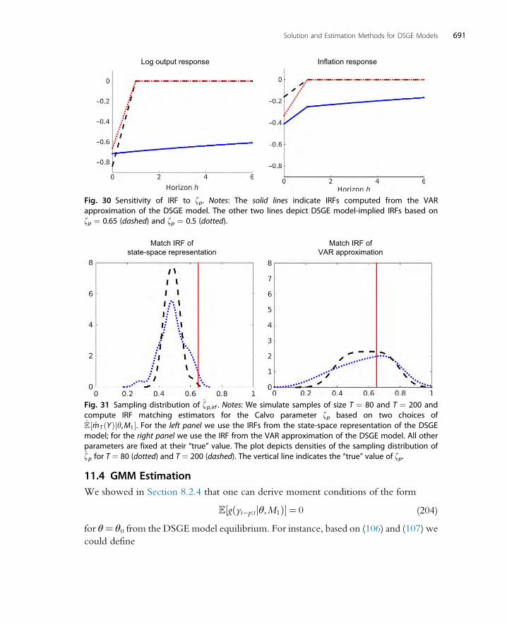
11.4 GMM EstimationWe showed in Section 8.2.4 that one can derive moment conditions of the form

½gðyt�p:tjθ,M1Þ�¼ 0 (204)

for θ¼ θ0 from the DSGEmodel equilibrium. For instance, based on (106) and (107) we

could define

Inflation responseLog output response

Fig. 30 Sensitivity of IRF to zp. Notes: The solid lines indicate IRFs computed from the VARapproximation of the DSGE model. The other two lines depict DSGE model-implied IRFs based onzp ¼ 0.65 (dashed) and zp ¼ 0.5 (dotted).

Match IRF ofstate-space representation

Match IRF ofVAR approximation

Fig. 31 Sampling distribution of zp, irf . Notes: We simulate samples of size T ¼ 80 and T ¼ 200 andcompute IRF matching estimators for the Calvo parameter zp based on two choices of½mT ðYÞjy,M1�. For the left panel we use the IRFs from the state-space representation of the DSGEmodel; for the right panel we use the IRF from the VAR approximation of the DSGE model. All otherparameters are fixed at their “true” value. The plot depicts densities of the sampling distribution ofzp for T ¼ 80 (dotted) and T ¼ 200 (dashed). The vertical line indicates the “true” value of zp.


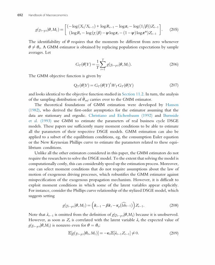
gðyt�p:tjθ,M1Þ¼� logðXt=Xt�1Þ+ logRt�1� logπt� logð1=βÞð ÞZt�1

logRt� logðγ=βÞ�ψ logπt�ð1�ψÞ logπ*ð ÞZt�1

� : (205)

The identifiability of θ requires that the moments be different from zero whenever

θ 6¼ θ0. A GMM estimator is obtained by replacing population expectations by sample

averages. Let

GTðθjYÞ¼ 1

T

XTt¼1

gðyt�p:tjθ,M1Þ: (206)

The GMM objective function is given by

QTðθjYÞ¼GTðθjYÞ0WTGT ðθjYÞ (207)

and looks identical to the objective function studied in Section 11.2. In turn, the analysis

of the sampling distribution of θmd carries over to the GMM estimator.

The theoretical foundations of GMM estimation were developed by Hansen

(1982), who derived the first-order asymptotics for the estimator assuming that the

data are stationary and ergodic. Christiano and Eichenbaum (1992) and Burnside

et al. (1993) use GMM to estimate the parameters of real business cycle DSGE

models. These papers use sufficiently many moment conditions to be able to estimate

all the parameters of their respective DSGE models. GMM estimation can also be

applied to a subset of the equilibrium conditions, eg, the consumption Euler equation

or the New Keynesian Phillips curve to estimate the parameters related to these equi-

librium conditions.

Unlike all the other estimators considered in this paper, the GMM estimators do not

require the researchers to solve the DSGEmodel. To the extent that solving the model is

computationally costly, this can considerably speed up the estimation process. Moreover,

one can select moment conditions that do not require assumptions about the law of

motion of exogenous driving processes, which robustifies the GMM estimator against

misspecification of the exogenous propagation mechanism. However, it is difficult to

exploit moment conditions in which some of the latent variables appear explicitly.

For instance, consider the Phillips curve relationship of the stylized DSGE model, which

suggests setting

gðyt�p:tjθ,M1Þ¼ π t�1�βπ t� κpðclsht�1Þ� �

Zt�1: (208)

Note that λt�1 is omitted from the definition of g(yt�p:tjθ,M1) because it is unobserved.

However, as soon as Zt is correlated with the latent variable λt the expected value of

g(yt�p:tjθ,M1) is nonzero even for θ ¼ θ0:

½gðyt�p:tjθ0,M1Þ� ¼�κ0½λt�1Zt�1� 6¼ 0: (209)


To the extent that λt is serially correlated, using higher-order lags of yt as instruments does

not solve the problem.av Recent work by Gallant et al. (2013) and Shin (2014) considers

extensions of GMM estimation to moment conditions with latent variables.

The recent literature on GMM estimation of DSGE models has focused on

identification-robust inference in view of the weak identification of Phillips curve and

monetary policy rule parameters. Generic identification problems in the context of mon-

etary policy rule estimation are highlighted in Cochrane (2011) and methods to conduct

identification-robust inference are developed inMavroeidis (2010). Identification-robust

inference for Phillips curve parameters is discussed in Mavroeidis (2005), Kleibergen and

Mavroeidis (2009), and Mavroeidis et al. (2014). Dufour et al. (2013) consider

identification-robust moment-based estimation of all of the equilibrium relationships

of a DSGE model.

12. BAYESIAN ESTIMATION TECHNIQUES

Bayesian inference is widely used in empirical work with DSGE models. The first papers

to estimate small-scale DSGE models using Bayesian methods were DeJong et al. (2000),

Schorfheide (2000), Otrok (2001), Fernandez-Villaverde and Rubio-Ramırez (2004),

and Rabanal and Rubio-Ramırez (2005). Subsequent papers estimated open-economy

DSGE models, eg, Lubik and Schorfheide (2006), and larger DSGE models tailored to

the analysis of monetary policy, eg, Smets and Wouters (2003) and Smets and Wouters

(2007). Because Bayesian analysis treats shock, parameter, and model uncertainty sym-

metrically by specifying a joint distribution that is updated in view of the observations

Y, it provides a conceptually appealing framework for decision making under uncer-

tainty. Levin et al. (2006) consider monetary policy analysis under uncertainty based

on an estimated DSGE model and the handbook chapter by Del Negro and

Schorfheide (2013) focuses on forecasting with DSGE models.

Conceptually, Bayesian inference is straightforward. A prior distribution is updated in

view of the sample information contained in the likelihood function. This leads to a pos-

terior distribution that summarizes the state of knowledge about the unknown parameter

vector θ. The main practical difficulty is the calculation of posterior moments and quan-

tiles of transformations h(�) of the parameter vector θ. The remainder of this section is

organized as follows.We provide a brief discussion of the elicitation of prior distributions

in Section 12.1. Sections 12.2 and 12.3 discuss two important algorithms to generate

parameter draws from posterior distributions: Markov chain Monte Carlo (MCMC)

and sequential Monte Carlo (SMC). Bayesian model diagnostics are reviewed in

av Under the assumption that λt follows an AR(1) process, one could quasi-difference the Phillips curve,

which would replace the term λt�1Zt�1 with Eλ,t�1Zt�1. If Zt�1 is composed of lagged observables dated

t � 2 and earlier, then the validity of the moment condition is restored.


Section 12.4. Finally, we discuss the recently emerging literature on limited-information

Bayesian inference in Section 12.5. Sections 12.1 and 12.3 are based on Herbst and

Schorfheide (2015), who provide a much more detailed exposition. Section 12.4 draws

from Del Negro and Schorfheide (2011).

12.1 Prior DistributionsThere is some disagreement in the Bayesian literature about the role of prior information

in econometric inference. Some authors advocate “flat” prior distributions that do not

distort the shape of the likelihood function, which raises two issues: first, most prior dis-

tributions are not invariant under parameter transformations. Suppose a scalar parameter

θ � U[�M,M]. If the model is reparameterized in terms of 1/θ, the implied prior is

no longer flat. Second, if the prior density is taken to be constant on the real line, say,

p(θ) ¼ c, then the prior is no longer proper, meaning the total prior probability mass

is infinite. In turn, it is no longer guaranteed that the posterior distribution is proper.

In many applications prior distributions are used to conduct inference in situations in

which the number of unknown parameters is large relative to the number of sample

observations. An example is a high-dimensional VAR. If the number of variables in

the VAR is n and the number of lags is p, then each equation has at least np unknown

parameters. For instance, a 4-variable VAR with p ¼ 4 lags has 16 parameters. If this

model is estimated based on quarterly post-Great Moderation and pre-Great Recession

data, the data-to-parameter ratio is approximately 6, which leads to very noisy parameter

estimates. A prior distribution essentially augments the estimation sample Y by artificial

observations Y * such that the model is estimated based on the combined sample (Y,Y *).Prior distributions can also be used to “regularize” the likelihood function by giving

the posterior density a more elliptical shape. Finally, a prior distribution can be used to

add substantive information about model parameters not contained in the estimation

sample θ to the inference problem. Bayesian estimation of DSGE models uses prior dis-

tributions mostly to add information contained in data sets other than Y and to smooth

out the likelihood function, down-weighing regions of the parameter space in which

implications of the structural model contradict nonsample information and the model

becomes implausible. An example would be a DSGE model with a likelihood that has

a local maximum at which the discount factor is, say, β ¼ 0.5. Such a value of β would

strongly contradict observations of real interest rates. A prior distribution that implies

that real interest rates are between 0% and 10% with high probability would squash

the undesirable local maximum of the likelihood function.

To the extent that the prior distribution is “informative” and affects the shape of the

posterior distribution, it is important that the specification of the prior distribution be

carefully documented. Del Negro and Schorfheide (2008) developed a procedure to con-

struct prior distributions based on information contained in presamples or in time series


that are not directly used for the estimation of the DSGE model. To facilitate the elic-

itation of a prior distribution it is useful to distinguish three groups of parameters: steady-

state-related parameters, exogenous shock parameters, and endogenous propagation

parameters.

In the context of the stylized DSGE model, the steady-state-related parameters are

given by β (real interest rate), π* (inflation), γ (output growth rate), and λ (labor share).A prior for these parameters could be informed by presample averages of these series. The

endogenous propagation parameters are ζp (Calvo probability of not being able to reop-

timize price) and ν (determines the labor supply elasticity). Micro-level information

about the frequency of price changes and labor supply elasticities can be used to specify

a prior distribution for these two parameters. Finally, the exogenous shock parameters are

the autocorrelation parameters ρ and the shock standard deviations σ.Because the exogenous shocks are latent, it is difficult to specify a prior distribution for

these parameters directly. However, it is possible to map beliefs about the persistence and

volatility of observables such as output growth, inflation, and interest rates into beliefs

about the exogenous shock parameters. This can be done using the formal procedure

described in Del Negro and Schorfheide (2008) or, informally, by generating draws of

θ from the prior distribution, simulating artificial observations from the DSGE model,

and computing the implied sample moments of the observables. If the prior predictive

distribution of these sample moments appears implausible, say, in view of sample statistics

computed from a presample of actual observations, then one can adjust the prior distri-

bution of the exogenous shock parameters and repeat the simulation until a plausible

prior is obtained. Table 7 contains an example of a prior distribution for our stylized

DSGE model. The joint distribution for θ is typically generated as a product of marginal

distributions for the elements (or some transformations thereof ) of the vector θ.aw In

most applications this product of marginals is truncated to ensure that the model has a

unique equilibrium.

12.2 Metropolis–Hastings AlgorithmDirect sampling from the posterior distribution of θ is unfortunately not possible. One

widely used algorithm to generate draws from p(θjY ) is the Metropolis–Hastings (MH)

algorithm, which belongs to the class of MCMC algorithms. MCMC algorithms

produce a sequence of serially correlated parameter draws θi, i ¼ 1,…,N with the prop-

erty that the random variables θi converge in distribution to the target posterior distri-

bution, which we abbreviate as

aw In high-dimensional parameter spaces it might be desirable to replace some of the θ elements by transfor-

mations, eg, steady states, that are more plausibly assumed to be independent. This transformation essen-

tially generates nonzero correlations for the original DSGE model parameters. Alternatively, the method

discussed in Del Negro and Schorfheide (2008) also generates correlations between parameters.


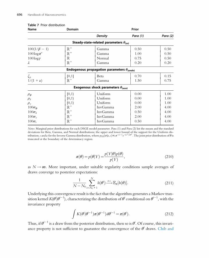
πðθÞ¼ pðθjYÞ¼ pðY jθÞpðθÞpðYÞ , (210)

as N !∞. More important, under suitable regularity conditions sample averages of

draws converge to posterior expectations:

1

N �N0

XNi¼N0 + 1

hðθiÞ�!a:s: π½hðθÞ�: (211)

Underlying this convergence result is the fact that the algorithm generates a Markov tran-

sition kernelK(θijθi�1), characterizing the distribution of θi conditional on θi�1, with the

invariance property ZKðθijθi�1Þπðθi�1Þdθi�1¼ πðθiÞ: (212)

Thus, if θi�1 is a draw from the posterior distribution, then so is θi. Of course, this invari-

ance property is not sufficient to guarantee the convergence of the θi draws. Chib and

Table 7 Prior distributionName Domain Prior

Density Para (1) Para (2)

Steady-state-related parameters θ(ss)

100(1/β � 1) + Gamma 0.50 0.50

100logπ� + Gamma 1.00 0.50

100logγ Normal 0.75 0.50

λ + Gamma 0.20 0.20

Endogenous propagation parameters θ(endo)

ζp [0,1] Beta 0.70 0.15

1/(1 + ν) + Gamma 1.50 0.75

Exogenous shock parameters θ(exo)

ρϕ [0,1) Uniform 0.00 1.00

ρλ [0,1) Uniform 0.00 1.00

ρz [0,1) Uniform 0.00 1.00

100σϕ + InvGamma 2.00 4.00

100σλ + InvGamma 0.50 4.00

100σz + InvGamma 2.00 4.00

100σr + InvGamma 0.50 4.00

Notes: Marginal prior distributions for each DSGE model parameter. Para (1) and Para (2) list the means and the standarddeviations for Beta, Gamma, and Normal distributions; the upper and lower bound of the support for the Uniform dis-tribution; s and ν for the Inverse Gamma distribution, where pIGðσjν, sÞ∝σ�ν�1e�νs2=2σ2 . The joint prior distribution of θ istruncated at the boundary of the determinacy region.


Greenberg (1995) provide an excellent introduction toMH algorithms and detailed text-

book treatments can be found, for instance, in Robert and Casella (2004) and Geweke

(2005).

12.2.1 The Basic MH AlgorithmThe key ingredient of the MH algorithm is a proposal distribution q(ϑjθi�1), which

potentially depends on the draw θi�1 in iteration i� 1 of the algorithm.With probability

α(ϑjθi�1) the proposed draw is accepted and θi¼ ϑ. If the proposed draw is not accepted,

then the chain does not move and θi ¼ θi�1. The acceptance probability is chosen to

ensure that the distribution of the draws converges to the target posterior distribution.

The algorithm takes the following form:

Algorithm 7 (Generic MH Algorithm). For i ¼ 1 to N:

1. Draw ϑ from a density q(ϑjθi�1).

2. Set θi ¼ ϑ with probability

αðϑjθi�1Þ¼ min 1,pðY jϑÞpðϑÞ=qðϑjθi�1Þ

pðY jθi�1Þpðθi�1ÞÞ=qðθi�1jϑÞ� �

and θi ¼ θi�1 otherwise.

Because pðθjYÞ∝pðY jθÞpðθÞ we can replace the posterior densities in the calculation of

the acceptance probabilities α(ϑjθi�1) with the product of the likelihood and prior, which

does not require the evaluation of the marginal data density p(Y ).

12.2.2 Random-Walk Metropolis–Hastings AlgorithmThe most widely used MH algorithm for DSGE model applications is the random walk

MH (RWMH) algorithm. The basic version of this algorithm uses a normal distribution

centered at the previous θi draw as the proposal density:

ϑjθi �N θi, c2Σ� �

: (213)

Given the symmetric nature of the proposal distribution, the acceptance probability

becomes

α¼ minpðϑjYÞ

pðθi�1jYÞ ,1� �

:

A draw, ϑ, is accepted with probability one if the posterior at ϑ has a higher value than theposterior at θi�1. The probability of acceptance decreases as the posterior at the candidate

value decreases relative to the current posterior.

To implement the RWMH, the user needs to specify c, and Σ. The proposal variancecontrols the relative variances and correlations in the proposal distribution. The sampler

can work very poorly if q is strongly at odds with the target distribution. A good choice


for Σ seeks to incorporate information from the posterior, to potentially capture the a

posteriori correlations among parameters. Obtaining this information can be difficult.

A popular approach, used in Schorfheide (2000), is to set Σ to be the negative of the

inverse Hessian at the mode of the log posterior, θ, obtained by running a numerical

optimization routine before running the MCMC algorithm. Using this as an estimate

for the covariance of the posterior is attractive, because it can be viewed as a large sample

approximation to the posterior covariance matrix.

Unfortunately, in many applications, the maximization of the posterior density is

tedious and the numerical approximation of the Hessian may be inaccurate. These prob-

lems may arise if the posterior distribution is very nonelliptical and possibly multimodal,

or if the likelihood function is replaced by a nondifferentiable particle filter approxima-

tion. In both cases, a (partially) adaptive approach may work well: First, generate a set of

posterior draws based on a reasonable initial choice for Σ, eg, the prior covariance matrix.

Second, compute the sample covariance matrix from the first sequence of posterior draws

and use it as Σ in a second run of the RWMH algorithm. In principle, the covariance

matrix Σ can be adjusted more than once. However, Σ must be fixed eventually to guar-

antee the convergence of the posterior simulator. Samplers that constantly (or automat-

ically) adjust Σ are known as adaptive samplers and require substantially more elaborate

theoretical justifications.

12.2.3 Numerical IllustrationWe generate a single sample of size T ¼ 80 from the stylized DSGE model using the

parameterization in Table 5. The DSGE model likelihood function is combined with

the prior distribution in Table 7 to form a posterior distribution. Draws from this pos-

terior distribution are generated using the RWMH described in the previous section.

The chain is initialized with a draw from the prior distribution. The covariance matrix

Σ is based on the negative inverse Hessian at the mode. The scaling constant c is set equal

to 0.075, which leads to an acceptance rate for proposed draws of 0.55.

The top panels of Fig. 32 depict the sequences of posterior draws of the Calvo param-

eter ζip and preference shock standard deviation σiϕ. It is apparent from the figure that the

draws are serially correlated. The draws for the standard deviation are strongly contam-

inated by the initialization of the chain, but they eventually settle to a range of 0.8–1.1.

The bottom panel depicts recursive means of the form

�hN jN0¼ 1

N �N0

XNi¼N0 + 1

hðθiÞ: (214)

To remove the effect of the initializationof theMarkovchain, it is common todrop the first

N0 draws from the computation of the posterior mean approximation. In the figure we set

N0 ¼ 7500 and N ¼ 37,500. Both recursive means eventually settle to a limit point.


The output of the algorithm is stochastic, which implies that running the algorithm

repeatedly will generate different numerical results. Under suitable regularity conditions

the recursive means satisfy a CLT. The easiest way to obtain a measure of numerical accu-

racy is to run the RWMH algorithm, say, fifty times using random starting points, and

compute the sample variance of �hN jN0across chains. Alternatively, one could compute a

heteroskedasticity and autocorrelation consistent (HAC) standard error estimate for�hN jN0

based on the output of a single chain.

Fig. 33 depicts univariate prior and posterior densities, which are obtained by apply-

ing a standard kernel density estimator to draws from the prior and posterior distribution.

In addition, one can also compute posterior credible sets based on the output of the

Recursive mean 1N−N0

Ni=N0+1Σ Recursive mean 1

N−N0

Ni=N0+1Σ

ζpi Draws σφ

i Draws

ζpi σφ

i

Fig. 32 Parameter draws from MH algorithm. Notes: The posterior is based on a simulated sample ofobservations of size T ¼ 80. The top panel shows the sequence of parameter draws and the bottompanel shows recursive means.


posterior sampler. For a univariate parameter, the shortest credible set is given by the

highest-posterior-density (HPD) set defined as

CSHPDðYÞ¼ θ pðθjYÞj � καf g, (215)

where κα is chosen to ensure that the credible set has the desired posterior coverage

probability.

12.2.4 BlockingDespite a careful choice of the proposal distribution q(�jθi�1), it is natural that the effi-

ciency of the MH algorithm decreases as the dimension of the parameter vector θincreases. The success of the proposed random walk move decreases as the dimension

d of the parameter space increases. One way to alleviate this problem is to break the

parameter vector into blocks. Suppose the dimension of the parameter vector θ is d.

A partition of the parameter space, B, is a collection of Nblocks sets of indices. These

sets are mutually exclusive and collectively exhaustive. Call the subvectors that cor-

respond to the index sets θb, b ¼ 1,…,Nblocks. In the context of a sequence of param-

eter draws, let θib refer to the b-th block of i-th draw of θ and let θi<b refer to the i-th

draw of all of the blocks before b and similarly for θi>b. Algorithm 8 describes a generic

Block MH algorithm.

Algorithm 8 (Block MH Algorithm). Draw θ0 2 Θ and then for i ¼ 1 to N:

1. Create a partition Bi of the parameter vector into Nblocks blocks θ1,…,θNblocksvia some

rule (perhaps probabilistic), unrelated to the current state of the Markov chain.

2. For b ¼ 1,…,Nblocks:

Posterior ζp Posterior σφ

0.7

Fig. 33 Prior and posterior densities. Notes: The dashed lines represent the prior densities, whereas thesolid lines correspond to the posterior densities of zp and sf. The posterior is based on a simulatedsample of observations of size T ¼ 80. We generate N ¼ 37,500 draws from the posterior and dropthe first N0 ¼ 7,500 draws.


(a) Draw ϑb � q(�j[θ<bi , θb

i�1, θ�bi�1]).

(b) With probability,

α¼ maxpð θi<b,ϑb,θ

i�1>b

� �jYÞqðθi�1b , jθi<b,ϑb,θ

i�1>b Þ

pðθi<b,θi�1b ,θi�1

>b jYÞqðϑbjθi<b,θi�1b ,θi�1

>b Þ,1

� �,

set θbi ¼ϑb, otherwise set θb

i ¼ θbi�1.

In order to make the Block MH algorithm operational, the researcher has to decide how

to allocate parameters to blocks in each iteration and how to choose the proposal distri-

bution qð � j θi<b,θi�1b ,θi�1

>b

� �Þ for parameters of block b.

A good rule of thumb, however, is that we want the parameters within a block, say, θb,to be as correlated as possible, while we want the parameters between blocks, say, θb andθ�b, to be as independent as possible, according to Robert and Casella (2004). Unfortu-

nately, picking the “optimal” blocks to minimize dependence across blocks requires a

priori knowledge about the posterior and is therefore often infeasible. Chib and

Ramamurthy (2010) propose grouping parameters randomly. Essentially, the user spec-

ifies howmany blocks to partition the parameter vector into and every iteration a new set

of blocks is constructed. Key to the algorithm is that the block configuration be indepen-

dent of the Markov chain. This is crucial for ensuring the convergence of the chain.

In order to tailor the block-specific proposal distributions, Chib and Ramamurthy

(2010) advocate using an optimization routine—specifically, simulated annealing—to

find the mode of the conditional posterior distribution. As in the RWMH-V algorithm,

the variance of the proposal distribution is based on the inverse Hessian of the conditional

log posterior density evaluated at the mode. Unfortunately, the tailoring requires many

likelihood evaluations that slow down the algorithm and a simpler procedure, such as

using marginal or conditional covariance matrices from an initial approximation of

the joint posterior covariance matrix, might be computationally more efficient.

12.2.5 Marginal Likelihood ApproximationsThe computations thus far do not rely on the marginal likelihood p(Y ), which appears in

the denominator of Bayes Theorem.Marginal likelihoods play an important role in asses-

sing the relative fit of models because they are used to turn prior model probabilities into

posterior probabilities. The most widely used marginal likelihood approximation in the

DSGE model literature is the modified harmonic mean estimator proposed by Geweke

(1999). This estimator is based on the identity

R f ðθÞpðYÞdθ¼

Zf ðθÞ

pðY jθÞpðθÞpðθjYÞdθ, (216)

where f(θ) has the property thatRf ðθÞdθ¼ 1. The identity is obtained by rewriting Bayes

Theorem, multiplying both sides with f(θ) and integrating over θ. Realizing that the


left-hand side simplifies to 1/p(Y ) and that the right-hand side can be approximated by a

Monte Carlo average we obtain

pHMðYÞ¼1

N

XNi¼1

f ðθiÞpðY jθiÞpðθiÞ

" #�1

, (217)

where the θi’s are drawn from the posterior p(θjY ). The function f(θ) should be chosen tokeep the variance of f(θi)/p(Y jθi)p(θi) small. Geweke (1999) recommends using for f(θ) atruncated normal approximation of the posterior distribution for θ that is computed from

the output of the posterior sampler. Alternative methods to approximate the marginal

likelihood are discussed in Chib and Jeliazkov (2001), Sims et al. (2008), and Ardia

et al. (2012). An and Schorfheide (2007) and Herbst and Schorfheide (2015) provide

accuracy comparisons of alternative methods.

12.2.6 ExtensionsThe basic estimation approach for linearized DSGE models has been extended in several

dimensions. Typically, the parameter space is restricted to a subspace in which a line-

arized model has a unique nonexplosive rational expectations solution (determinacy).

Lubik and Schorfheide (2004) relax this restriction and also consider the region of

the parameter space in which the solution is indeterminate. By computing the posterior

probability of parameter values associated with indeterminacy, they are able to conduct

a posterior odds assessment of determinacy vs indeterminacy. Justiniano and Primiceri

(2008) consider a linearized DSGE model with structural shocks that exhibit stochastic

volatility and develop an MCMC algorithm for posterior inference. A further extension

is provided by Curdia et al. (2014), who also allow for shocks that, conditional on the

volatility process, have a fat-tailed student-t distribution to capture extreme events such

as the Great Recession. Schorfheide (2005a) and Bianchi (2013) consider the estimation

of linearized DSGE models with regime switching in the coefficients of the state-space

representation.

M€uller (2012) provides an elegant procedure to assess the robustness of posterior

inference to shifts in the mean of the prior distribution. One of the attractive features of

his procedure is that the robustness checks can be carried out without having to reestimate

theDSGEmodelunder alternativepriordistributions.Koopet al. (2013)propose somediag-

nostics that allow users to determine the extent towhich the likelihood function is informa-

tive about the DSGE model parameters. In a nutshell, the authors recommend examining

whether thevarianceofmarginalposteriordistributions shrinks at the rateT�1 (in a stationary

model) if the number of observations is increased in a simulation experiment.

12.2.7 Particle MCMCWe now turn to the estimation of fully nonlinear DSGE models. As discussed in

Section 10, for nonlinear DSGE models the likelihood function has to be approximated


by a nonlinear filter. Embedding a particle filter approximation into an MCMC sampler

leads to a so-called particle MCMC algorithm.We refer to the combination of a particle-

filter approximated likelihood and the MH algorithm as a PFMH algorithm. This idea

was first proposed for the estimation of nonlinear DSGE models by Fernandez-

Villaverde and Rubio-Ramırez (2007). The theory underlying the PFMH algorithm

is developed in Andrieu et al. (2010). Flury and Shephard (2011) discuss non-DSGE

applications of particle MCMC methods in econometrics. The modification of

Algorithm 7 is surprisingly simple: one only has to replace the exact likelihood function

p(Y jθ) with the particle filter approximation pðY jθÞ.Algorithm 9 (PFMH Algorithm). For i ¼ 1 to N:

1. Draw ϑ from a density q(ϑjθi�1).

2. Set θi ¼ ϑ with probability

αðϑjθi�1Þ¼ min 1,pðY jϑÞpðϑÞ=qðϑjθi�1Þ

pðY jθi�1Þpðθi�1Þ=qðθi�1jϑÞ� �

and θi ¼ θi�1 otherwise. The likelihood approximation p(Yjϑ) is computed using

Algorithm 6.

The surprising implication of the theory developed in Andrieu et al. (2010) is that the

distribution of draws generated by Algorithm 9 from the PFMH algorithm that replaces

p(Y jθ) with pðY jθÞ in fact does converge to the exact posterior. The replacement of the

exact likelihood function by the particle-filter approximation generally increases the per-

sistence of the Markov chain and makes Monte Carlo approximations less accurate; see

Herbst and Schorfheide (2015) for numerical illustrations. Formally, the key requirement

is that the particle-filter approximation provide an unbiased estimate of the likelihood

function. In practice it has to be ensured that the variance of the numerical approximation

is small relative to the expected magnitude of the differential between p(Y jθi�1) and p(Y

jϑ) in an ideal version of the algorithm in which the likelihood could be evaluated

exactly. Thus, before embedding the particle-filter approximation into a likelihood func-

tion, it is important to assess its accuracy for low- and high-likelihood parameter values.

12.3 SMC MethodsSequential Monte Carlo (SMC) techniques to generate draws from posterior distribu-

tions of a static parameter θ are emerging as an attractive alternative to MCMCmethods.

SMC algorithms can be easily parallelized and, properly tuned, may produce more accu-

rate approximations of posterior distributions than MCMC algorithms. Chopin (2002)

showed how to adapt the particle filtering techniques discussed in Section 10.3 to

conduct posterior inference for a static parameter vector. Textbook treatments of

SMC algorithms can be found, for instance, in Liu (2001) and Capp�e et al. (2005).


The first paper that applied SMC techniques to posterior inference in a small-scale

DSGE models was Creal (2007). Herbst and Schorfheide (2014) develop the algorithm

further, provide some convergence results for an adaptive version of the algorithm build-

ing on the theoretical analysis of Chopin (2004), and show that a properly tailored SMC

algorithm delivers more reliable posterior inference for large-scale DSGE models with a

multimodal posterior than the widely used RWMH-V algorithm. Creal (2012) provides

a recent survey of SMC applications in econometrics. Durham and Geweke (2014) show

how to parallelize a flexible and self-tuning SMC algorithm for the estimation of time

series models on graphical processing units (GPU). The remainder of this section draws

heavily from the more detailed exposition in Herbst and Schorfheide (2014, 2015).

SMC combines features of classic importance sampling and modern MCMC

techniques. The starting point is the creation of a sequence of intermediate or bridge

distributions fπnðθÞgNϕ

n¼0 that converge to the target posterior distribution, ie,

πNϕðθÞ¼ πðθÞ. At any stage the posterior distribution πn(θ) is represented by a swarm

of particles fθin,WingNi¼1 in the sense that the Monte Carlo average

�hn,N ¼ 1

N

XNi¼1

WinhðθinÞ!

a:s:πn ½hðθnÞ�: (218)

The bridge distributions can be generated either by taking power transformations of the

entire likelihood function, that is, ½pðY jθÞ�ϕn , where ϕn" 1, or by adding observations tothe likelihood function, that is, pðY1:tn jθÞ, where tn" T. We refer to the first approach as

likelihood tempering and the second approach as data tempering. Formally, the

sequences of bridge distributions are defined as (likelihood tempering)

πnðθÞ¼ ½pðY jθÞ�ϕnpðθÞR ½pðY jθÞ�ϕnpðθÞdθ n¼ 0,…,Nϕ, ϕn " 1, (219)

and (data tempering, writing tn ¼ bϕnTc)

πðDÞn ðθÞ¼ pðY1:bϕnTcÞpðθÞR

pðY1:bϕnTcÞpðθÞdθn¼ 0,…,Nϕ, ϕn " 1, (220)

respectively. While data tempering is attractive in sequential applications, eg, real-time

forecasting, likelihood tempering generally leads to more stable posterior simulators for

two reasons: First, in the initial phase it is possible to add information that corresponds to a

fraction of an observation. Second, if the latter part of the sample contains influential

observations that drastically shift the posterior mass, data tempering may have difficulties

adapting to the new information.

12.3.1 The SMC AlgorithmThe algorithm can be initializedwith draws from the prior density p(θ), provided the priordensity is proper. For the prior inTable 7 it is possible to directly sample independent draws


θi0 from themarginal distributions of theDSGEmodel parameters.One can add an accept-

reject step that eliminates parameter draws for which the linearizedmodel does not have a

unique stable rational expectations solution.The initialweightsWi0 canbe set equal to one.

We adopt the convention that the weights are normalized to sum to N.

The SMC algorithm proceeds iteratively from n ¼ 0 to n ¼ Nϕ. Starting from stage

n � 1 particles fθin�1,Win�1gNi¼1 each stage n of the algorithm consists of three steps:

correction, that is, reweighting the stage n � 1 particles to reflect the density in iteration

n; selection, that is, eliminating a highly uneven distribution of particle weights (degener-

acy) by resampling the particles; and mutation, that is, propagating the particles forward

using a Markov transition kernel to adapt the particle values to the stage n bridge density.

Algorithm 10 (Generic SMC Algorithm with Likelihood Tempering).

1. Initialization. (ϕ0 ¼ 0). Draw the initial particles from the prior: θi0 �iidp

p(θ)and W 0

i ¼ 1, i ¼ 1,…,N.

2. Recursion. For n ¼ 1,…,Nϕ,

(a) Correction.Reweight the particles from stage n� 1 by defining the incremen-

tal weights

w� i

n¼ ½pðY jθin�1Þ�ϕn�ϕn�1 (221)

and the normalized weights

W� i

n ¼w� i

nWin�1

1

N

XN

i¼1w� inW

in�1,

i¼ 1,…,N : (222)

(b) Selection (Optional). Resample the particles via multinomial resampling. Let

{θ}i¼1N denoteN iid draws from a multinomial distribution characterized by support

points and weights {θn�1i ,W

�ni }i¼1

N and set Wni ¼ 1.

(c) Mutation. Propagate the particles {θ i,Wni } via NMH steps of an MH algorithm

with transition density θni � Kn(θnjθni ; ζn) and stationary distribution πn(θ). An

approximation of πn [h(θ)] is given by

�hn,N ¼ 1

N

XNi¼1

hðθinÞWin: (223)

3. For n ¼ Nϕ (ϕNϕ¼ 1) the final importance sampling approximation of π[h(θ)] is

given by:

�hNϕ,N ¼XNi¼1

hðθiNϕÞWi

Nϕ: (224)

The correction step is a classic importance sampling step, in which the particle weights are

updated to reflect the stage n distribution πn(θ). Because this step does not change the

particle value, it is typically not necessary to reevaluate the likelihood function.


The selection step is optional. On the one hand, resampling adds noise to the Monte

Carlo approximation, which is undesirable. On the other hand, it equalizes the particle

weights, which increases the accuracy of subsequent importance sampling approxima-

tions. The decision of whether or not to resample is typically based on a threshold rule

for the variance of the particle weights. As for the particle filter in Section 10.3, we can

define an effective particle sample size as:

dESSn¼N=1

N

XNi¼1

ðW� inÞ2

!(225)

and resample whenever dESSn is less thatN/2 orN/4. In the description of Algorithm 10

we consider multinomial resampling. Other, more efficient resampling schemes are dis-

cussed, for instance, in the books by Liu (2001) or Capp�e et al. (2005) (and references

cited therein).

Themutation step changes the particle values. In the absence of the mutation step, the

particle values would be restricted to the set of values drawn in the initial stage from the

prior distribution. This would clearly be inefficient, because the prior distribution is a

poor proposal distribution for the posterior in an importance sampling algorithm. As

the algorithm cycles through the Nϕ phases, the particle values successively adapt to

the shape of the posterior distribution. The key feature of the transition kernel

Knðθnjθn;ζnÞ is the invariance property:

πnðθnÞ¼Z

Knðθnjθn;ζnÞπnðθnÞdθn: (226)

Thus, if θi

n is a draw from πn, then so is θin. The mutation step can be implemented by

using one or more steps of the RWMH algorithm described in Section 12.2.2. The prob-

ability of mutating the particles can be increased by blocking or by iterating the RWMH

algorithm over multiple steps. The vector ζn summarizes the tuning parameters, eg, c and

Σ of the RWMH algorithm.

The SMC algorithm produces as a by-product an approximation of the marginal like-

lihood. It can be shown that

pSMCðYÞ¼YNϕ

n¼1

1

N

XNi¼1

w� inW

in�1

!

converges almost surely to p(Y ) as the number of particles N !∞.

12.3.2 Tuning the SMC AlgorithmThe implementation of the SMC algorithm requires the choice of several tuning con-

stants. The most important choice is the number of particles N. As shown in Chopin

(2004), Monte Carlo averages computed from the output of the SMC algorithm satisfy


a CLT as the number of particles increases to infinity. This means that the variance of the

Monte Carlo approximation decreases at the rate 1/N. The user has to determine the

number of bridge distributionsNϕ and the tempering schedule ϕn. Based on experiments

with a small-scale DSGE model, Herbst and Schorfheide (2015) recommend a convex

tempering schedule of the form ϕn ¼ (n/Nϕ)λ with λ � 2. Durham and Geweke

(2014) recently developed a self-tuning algorithm that chooses the sequence ϕn adap-

tively as the algorithm cycles through the stages.

The mutation step requires the user to determine the number of MH steps NMH and

the number of parameter blocks. The increased probability of mutation raises the accu-

racy but unfortunately, the number of likelihood evaluations increases as well, which

slows down the algorithm. The scaling constant c and the covariance matrix Σ can be

easily chosen adaptively. Based on the MH rejection frequency, c can be adjusted to

achieve a target rejection rate of approximately 25–40%. For Σn one can use an approx-

imation of the posterior covariance matrix computed at the end of the stage n

correction step.

To monitor the accuracy of the SMC approximations Durham and Geweke (2014)

suggest creating H groups of N particles and setting up the algorithm so that there is no

communication across groups. This leads to HMonte Carlo approximations of posterior

moments of interest. The across-group standard deviation of within-group Monte Carlo

averages provides a measure of numerical accuracy. Parallelization of the SMC algorithm

is relatively straightforward because the mutation step and the computation of the incre-

mental weights in the correction step can be carried out in parallel on multiple processors,

each of which is assigned a group of particles. In principle, the exact likelihood function

can be replaced by a particle-filter approximation, which leads to an SMC2 algorithm,

developed by Chopin et al. (2012) and discussed in more detail in the context of DSGE

models in Herbst and Schorfheide (2015).

12.3.3 Numerical IllustrationWenow illustrate the SMCmodel in the context of the stylizedDSGEmodels. The setup

is similar to the one in Section 12.2.3.We generateT¼ 80 observations using the param-

eters listed in Table 5 and use the prior distribution given in Table 7. The algorithm is

configured as follows. We use N ¼ 2048 particles and Nϕ ¼ 500 tempering stages.

We set λ ¼ 3, meaning that we add very little information in the initial stages to ensure

that the prior draws adapt to the shape of the posterior. We use one step of a single-block

RWMH algorithm in the mutation step and choose c and Σn adaptively as described in

Herbst and Schorfheide (2014). The target acceptance rate for the mutation step is 0.25.

Based on the output of the SMC algorithm, we plot marginal bridge densities πn(�) for theprice stickiness parameter ζp and the shock standard deviation σϕ in Fig. 34. The initial setof particles is drawn from the prior distribution. As ϕn increases to one, the distribution

concentrates. The final stage approximates the posterior distribution.


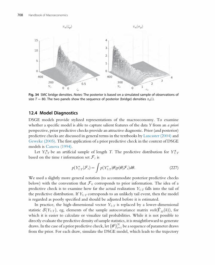
12.4 Model DiagnosticsDSGE models provide stylized representations of the macroeconomy. To examine

whether a specific model is able to capture salient features of the data Y from an a priori

perspective, prior predictive checks provide an attractive diagnostic. Prior (and posterior)

predictive checks are discussed in general terms in the textbooks by Lancaster (2004) and

Geweke (2005). The first application of a prior predictive check in the context of DSGE

models is Canova (1994).

Let Y1:T* be an artificial sample of length T. The predictive distribution for Y *1:Tbased on the time t information set F t is

pðY �1:T jF tÞ¼

ZpðY �

1:T jθÞpðθjF tÞdθ: (227)

We used a slightly more general notation (to accommodate posterior predictive checks

below) with the convention that F 0 corresponds to prior information. The idea of a

predictive check is to examine how far the actual realization Y1:T falls into the tail of

the predictive distribution. If Y1:T corresponds to an unlikely tail event, then the model

is regarded as poorly specified and should be adjusted before it is estimated.

In practice, the high-dimensional vector Y1:T is replaced by a lower-dimensional

statistic SðY1:TÞ, eg, elements of the sample autocovariance matrix vechðΓyyðhÞÞ, forwhich it is easier to calculate or visualize tail probabilities. While it is not possible to

directly evaluate the predictive density of sample statistics, it is straightforward to generate

draws. In the case of a prior predictive check, let fθigNi¼1 be a sequence of parameter draws

from the prior. For each draw, simulate the DSGE model, which leads to the trajectory

πn(ζp) πn(σφ)

Fig. 34 SMC bridge densities. Notes: The posterior is based on a simulated sample of observations ofsize T ¼ 80. The two panels show the sequence of posterior (bridge) densities pn(�).


Y �i1:T . For each of the simulated trajectories, compute the sample statistic Sð � Þ, which

leads to a draw from the predictive density.

For a posterior predictive check one equates F t with the sample Y1:T. The posterior

predictive check examines whether the estimated DSGE model captures the salient fea-

tures of the sample. A DSGEmodel application can be found in Chang et al. (2007), who

examine whether versions of an estimated stochastic growthmodel are able to capture the

variance and the serial correlation of hours worked.

12.5 Limited Information Bayesian InferenceBayesian inference requires a likelihood function p(Y jθ). However, as discussed in

Section 11, many of the classical approaches to DSGE model estimation,

eg, (generalized) methods of moments and impulse response function matching, do

not utilize the likelihood function of the DSGE model, in part because there is some

concern about misspecification. These methods are referred to as limited-information

(instead of full information) techniques. This subsection provides a brief survey of

Bayesian approaches to limited-information inference.

12.5.1 Single-Equation EstimationLubik and Schorfheide (2005) estimate monetary policy rules for small open economy

models by augmenting the policy rule equation with a vector-autoregressive law of

motion for the endogenous regressors, eg, the output gap and inflation in the case of

our stylized model. This leads to a VAR for output, inflation, and interest rates, with

cross-coefficient restrictions that are functions of the monetary policy rule parameters.

The restricted VAR can be estimated with standard MCMC techniques. Compared

to the estimation of a fully specified DSGE model, the limited-information approach

robustifies the estimation of the policy rule equation against misspecification of the pri-

vate sector’s behavior. Kleibergen andMavroeidis (2014) apply a similar technique to the

estimation of a New Keynesian Phillips curve. Their work focuses on the specification of

prior distributions that regularize the likelihood function in settings in which the sample

only weakly identifies the parameters of interest, eg, the slope of the New Keynesian

Phillips curve.

12.5.2 Inverting a Sampling DistributionSuppose one knows the sampling distribution pðθjθÞ of an estimator θ. Then, instead ofupdating beliefs conditional on the observed sampleY, one could update the beliefs about

θ based on the realization of θ:

pðθjθÞ¼ pðθjθÞpðθÞRpðθjθÞpðθÞ : (228)


This idea dates back at least to Pratt et al. (1965) and is useful in situations in which a

variety of different distributions for the sample Y lead to the same distribution of the

estimator θ. The drawback of this approach is that a closed-form representation of the

density pðθjθÞ is typically not available.

In practice one could use a simulation-based approximation of pðθjθÞ, which is an

idea set forth by Boos and Monahan (1986). Alternatively, one could replace the

finite-sample distribution with a limit distribution, eg,ffiffiffiffiT

p ðθT �θTÞjθT¼)N 0,V ðθÞð Þ, (229)

where the sequence of “true” parameters θT converges to θ. This approach is consideredby Kwan (1999). In principle θT could be any of the frequentist estimators studied in

Section 11 for which we derived an asymptotic distribution, including theMD estimator,

the IRF matching estimator, or the GMM estimator. However, in order for the resulting

limited-information posterior to be meaningful, it is important that the convergence to

the asymptotic distribution be uniform in θ, which requires (229) to hold for each

sequence θT!θ. A uniform convergence to a normal distribution is typically not attain-

able as θT approaches the boundary of the region of the parameter space in which the time

series Y1:T is stationary.

Rather than making statements about the approximation of the limited-information

posterior distribution pðθjθÞ, M€uller (2013) adopts a decision-theoretic framework and

shows that decisions based on the quasi-posterior that is obtained by inverting the limit

distribution of θT jθ are asymptotically optimal (in the sense that they minimize expected

loss) under fairly general conditions. Suppose that the likelihood function of a DSGE

model is misspecified. In this case the textbook analysis of the ML estimator in

Section 11.1 has to be adjusted as follows. The information matrix equality that ensures

that k�r2θ‘T ðθjYÞ�Iðθ0Þ k converges to zero is no longer satisfied. If we let

D¼ plimT!∞�r2θ‘TðθjYÞ, then the asymptotic variance of the ML estimator takes

the sandwich form DIðθ0ÞD0. Under the limited-information approach coverage sets

for individual DSGE model parameters would be computed based on the diagonal

elements of DIðθ0ÞD0, whereas under a full-information Bayesian approach with mis-

specified likelihood function, the coverage sets would (asymptotically) be based on

I�1ðθ0Þ. Thus, the limited-information approach robustifies the coverage sets against

model misspecification.

Instead of inverting a sampling distribution of an estimator, one could also invert the

sampling distribution of some auxiliary sample statistic φðYÞ. Not surprisingly, the main

obstacle is the characterization of the distribution φjθ. A collection of methods referred to

as approximate Bayesian computations (ABC) use a simulation approximation of pðφjθÞand they could be viewed as a Bayesian version of indirect inference. These algorithms

target


pδABCðθ, φ*jφÞ∝pðφ*jθÞpðθÞfk φ*� φ k� δg, (230)

where φ refers to the auxiliary statistic computed from the observed data, φ* is the aux-iliary statistic computed from data simulated from the model conditional on a parameter

θ, and δ is the level of tolerance for discrepancies between model-simulated and observed

statistics. To date, there are few applications of ABC in econometrics. Forneron and Ng

(2015) discuss the relationship between ABC and the simulated MD estimators intro-

duced in Section 11.2 and Scalone (2015) explores a DSGE model application.

12.5.3 Limited-Information Likelihood FunctionsKim (2002) constructs a limited-information likelihood function from the objective

function of an extremum estimator. For illustrative purposes we consider the GMM

estimator discussed in Section 11.4, but the same idea can also be applied to the MD

estimator and the IRF matching estimator. Suppose the data are generated under the

probability measure and at θ ¼ θ0 the following GMMmoment condition is satisfied:

½gðyt�p:tjθ0Þ� ¼ 0. The sample objective function QT(θjY ) for the resulting GMM

estimator based on a weight matrixWwas given in (207). Assuming uniform integrability

of the sample objective function

limT!∞

½QTðθ0jYÞ� ¼ r (231)

where r is the number of overidentifying moment conditions (meaning the difference

between the number of moments stacked in the vector g(�) and the number of elements

of the parameter vector θ).Let PðθÞ denote the collection of probability distributions that satisfy the moment

conditions in the following sense:

PðθÞ¼ P j limT!∞

P ½TQTðθjYÞ� ¼ r

� �: (232)

PðθÞ cannot be used directly for likelihood-based inference because it comprises a col-

lection of probability distributions indexed by θ. To obtain a unique distribution for eachθ, Kim (2002) projects the “true” distribution onto the set PðθÞ using the Kullback–Leibler discrepancy as the metric:

P*ðY jθÞ¼ argminP2PðθÞRlogðdP=dÞdP: (233)

The solution takes the convenient form

p*ðY jθÞ∝ exp �1

2QT ðθjYÞ

� �, (234)

where p*ðY jθÞ¼ dP=d is the Radon–Nikodym derivative of P with respect to .


Kim’s (2002) results suggest that the frequentist objective functions of Sections

11.2–11.4 can be combined with a prior density and used for (limited information)

Bayesian inference. The posterior mean

θ¼Rθexp �1

2QT ðθjYÞ

� �pðθÞdθ

Rexp �1

2QT ðθjYÞ

� �pðθÞdθ

(235)

resembles the LT estimator discussed in Section 11.2. The main difference is that the LT

estimator was interpreted from a frequentist perspective, whereas the quasi-posterior

based on p*(Y jθ) and statistics such as the posterior mean are meant to be interpreted

from a Bayesian perspective. This idea has been recently exploited by Christiano et al.

(2010) to propose a Bayesian IRF matching estimator. An application to an asset pricing

model is presented in Gallant (2015) and an extension to models with latent variables is

provided in Gallant et al. (2013). Inoue and Shintani (2014) show that the limited infor-

mation marginal likelihood

p*ðY jMÞ¼Z

p*ðY jθ,MÞpðθÞdθ

can be used as a model selection criterion that asymptotically is able to select a correct

model specification.

12.5.4 Nonparametric Likelihood FunctionsThere is also a literature on nonparametric likelihood functions that are restricted to sat-

isfy model-implied moment conditions. Lazar (2003) and Schennach (2005) use empir-

ical likelihood functions, which, roughly speaking assign probability pt to observation ytsuch that the likelihood function is written as

QTt¼1pt, at least if the data are iid. One then

imposes the side constraintPT

t¼1ptgðyt�p:tjθÞ¼ 0 and concentrates out pt probabilities to

obtain a profile objective function that only depends on θ. This method is designed for iid

data and possible models in which g(yt�p:tjθ) is a martingale difference sequence.

Kitamura and Otsu (2011) propose to using a Dirichlet process to generate a prior for

the distribution of Y1:T and then project this distribution on the set of distributions that

satisfies the moment restrictions. Shin (2014) uses a Dirichlet process mixture and

provides a time series extension.

13. CONCLUSION

Over the past two decades the development and application of solution and estimation

methods for DSGEmodels have experienced tremendous growth. Part of this growth has

been spurred by central banks, which have included DSGE models in their suites of


models used for forecasting and policy analysis. The rapid rise of computing power has

enabled researchers to study more and more elaborate model specifications. As we have

beenwriting this chapter, newmethods have been developed and novel applications have

been explored. While it is impossible to provide an exhaustive treatment of such a

dynamic field, we hope that this chapter provides a thorough training for those who

are interested in working in this area, offers a good overview of the state of the art as

of 2015, and inspires innovative research that expands the frontier of knowledge.

ACKNOWLEDGMENTSJ.F.-V. and J.F.R.-R. gratefully acknowledges financial support from the National Science Foundation

under Grant SES 1223271. F.S. gratefully acknowledges financial support from the National Science Foun-

dation under Grant SES 1424843. Minsu Chang, Eugenio Rojas, and Jacob Warren provided excellent

research assistance. We thank our discussant Serguei Maliar, the editors John Taylor and Harald Uhlig, John

Cochrane, Michael Curran, Oren Levintal, Ben Moll, Eric Swanson, and the participants at the Handbook

Conference hosted by the Hoover Institution for helpful comments and suggestions. Computer code to

implement the solution and estimation techniques discussed in this chapter is available on the authors’

websites.

REFERENCESAldrich, E.M., 2014. GPU computing in economics. In: Schmedders, K., Judd, K.L. (Eds.), Handbook of

Computational Economics, vol. 3. Elsevier, Amsterdam, pp. 557–598.Aldrich, E.M., Kung, H., 2011. Computational methods for production-based asset pricing models with

recursive utility. Economic Research Initiatives at Duke (ERID) Working Paper Series 87.Aldrich, E.M., Fernandez-Villaverde, J., Gallant, A.R., Rubio-Ramırez, J.F., 2011. Tapping the supercom-

puter under your desk: solving dynamic equilibrium models with graphics processors. J. Econ. Dyn.Control 35, 386–393.

Algan, Y., Allais, O., Den Haan, W.J., Rendahl, P., 2014. Solving and simulating models with heteroge-neous agents and aggregate uncertainty. In: Schmedders, K., Judd, K.L. (Eds.), Handbook of Compu-tational Economics, vol. 3. Elsevier, Amsterdam, pp. 277–324.

Altig, D., Christiano, L., Eichenbaum, M., Linde, J., 2011. Firm-specific capital, nominal rigidities and thebusiness cycle. Rev. Econ. Dyn. 14 (2), 225–247. http://ideas.repec.org/a/red/issued/09-191.html.

Altug, S., 1989. Time-to-build and aggregate fluctuations: some new evidence. Int. Econ. Rev. 30 (4),889–920.

Alvarez, F., Jermann, U.J., 2004. Using asset prices to measure the cost of business cycles. J. Polit. Econ.112, 1223–1256.

An, S., Schorfheide, F., 2007. Bayesian analysis of DSGE models. Econ. Rev. 26 (2-4), 113–172. http://dx.doi.org/10.1080/07474930701220071.

Anderson, E.W., Hansen, L.P., McGrattan, E.R., Sargent, T.J., 1996. On the mechanics of forming andestimating dynamic linear economies. In: Amman, H.M., Kendrick, D.A., Rust, J. (Eds.), Handbookof Computational Economics, vol. 1. Elsevier, Amsterdam, pp. 171–252.

Andreasen, M.M., 2013. Non-linear DSGE models and the central difference Kalman filter. J. Appl. Econ.28 (6), 929–955.

Andreasen, M.M., Fernandez-Villaverde, J., Rubio-Ramırez, J.F., 2013. The pruned state-space system fornonlinear DSGE models: theory and empircal applications. NBER Working 18983.

Andrews, I., Mikusheva, A., 2015. Maximum likelihood inference in weakly identified DSGE models.Quant. Econ 6 (1), 123–152.


http://refhub.elsevier.com/S1574-0048(16)00007-0/rf0010










http://ideas.repec.org/a/red/issued/09-191.html

http://ideas.repec.org/a/red/issued/09-191.html





http://dx.doi.org/10.1080/07474930701220071

http://dx.doi.org/10.1080/07474930701220071










Andrieu, C., Doucet, A., Holenstein, R., 2010. ParticleMarkov chainMonte Carlo methods. J. R. Stat. Soc.Ser. B 72 (3), 269–342.

Ardia, D., Bast€urk, N., Hoogerheide, L., van Dijk, H.K., 2012. A comparative study of Monte Carlomethods for efficient evaluation of marginal likelihood. Comput. Stat. Data Anal. 56 (11), 3398–3414.

Arulampalam, S., Maskell, S., Gordon, N., Clapp, T., 2002. A tutorial on particle filters for online nonlinear/non-gaussian Bayesian tracking. IEEE Trans. Signal Proc. 50 (2), 174–188.

Aruoba, S.B., Schorfheide, F., 2015. Inflation during and after the zero lower bound.Manuscript, Universityof Maryland.

Aruoba, S.B., Fernandez-Villaverde, J., Rubio-Ramırez, J.F., 2006. Comparing solution methods fordynamic equilibrium economies. J. Econ. Dyn. Control 30 (12), 2477–2508.

Barthelmann, V., Novak, E., Ritter, K., 2000. High dimensional polynomial interpolation on sparse grids.Adv. Comput. Math. 12, 273–288.

Bastani, H., Guerrieri, L., 2008. On the application of automatic differentiation to the likelihood function fordynamic general equilibrium models. In: Bischof, C.H., B€ucker, H.M., Hovland, P., Naumann, U.,Utke, J. (Eds.), Advances in Automatic Differentiation: Lecture Notes in Computational Scienceand Engineering, vol. 64. Springer, pp. 303–313.

Bender, C.M., Orszag, S.A., 1999. Advanced Mathematical Methods for Scientists and Engineers: Asymp-totic Methods and Perturbation Theory. Springer.

Benigno, P., Woodford, M., 2004. Optimal monetary and fiscal policy: a linear-quadratic approach.In: NBER Macroeconomics Annual 2003, vol. 18. MIT Press, Cambridge, MA, pp. 271–364.

Bernanke, B.S., Gertler, M., 1989. Agency costs, net worth, and business fluctuations. Am. Econ. Rev.79 (1), 14–31.

Bernanke, B.S., Gertler, M., Gilchrist, S., 1999. The financial accelerator in a quantitative business cycleframework. In: Taylor, J.B., Woodford, M. (Eds.), Handbook of Macroeconomics, vol. 1. Elsevier,pp. 1341–1393.

Bianchi, F., 2013. Regime switches, agents’ beliefs, and post-world war II U.S. macroeconomic dynamics.Rev. Econ. Stud. 80 (2), 463–490.

Blanchard, O.J., Kahn, C.M., 1980. The solution of linear difference models under rational expectations.Econometrica 48 (5), 1305–1312.

Bloom, N., 2009. The impact of uncertainty shocks. Econometrica 77, 623–685.Bocola, L., 2015. The pass-through of sovereign risk. Manuscript, Northwestern University.Boos, D.D., Monahan, J.F., 1986. Bootstrap methods using prior information. Biometrika 73 (1), 77–83.Boyd, J.P., 2000. Chebyshev and Fourier Spectral Methods. Dover.Boyd, J.P., Petschek, R.G., 2014. The relationships between Chebyshev, Legendre and Jacobi polynomials:

the generic superiority of Chebyshev polynomials and three important exceptions. J. Sci. Comput.59, 1–27.

Brenner, S., Scott, R., 2008. The Mathematical Theory of Finite Element Methods. Springer Verlag.Brown, D.B., Smith, J.E., Peng, S., 2010. Information relaxations and duality in stochastic dynamic

programs. Operat. Res. 58 (4), 785–801.Brumm, J., Scheidegger, S., 2015. Using adaptive sparse grids to solve high-dimensional dynamic models.

Manuscript, University of Zurich.Bungartz, H.J., Griebel, M., 2004. Sparse grids. Acta Numer. 13, 147–269.Burnside, C., Eichenbaum, M., Rebelo, S., 1993. Labor hoarding and the business cycle. J. Polit. Econ.

101 (2), 245–273. http://ideas.repec.org/a/ucp/jpolec/v101y1993i2p245-73.html.Cai, Y., Judd, K.L., 2014. Advances in numerical dynamic programming and new applications.

In: Schmedders, K., Judd, K.L. (Eds.), Handbook of Computational Economics, vol. 3. Elsevier,pp. 479–516.

Caldara, D., Fernandez-Villaverde, J., Rubio-Ramırez, J.F., Yao,W., 2012. Computing DSGEmodels withrecursive preferences and stochastic volatility. Rev. Econ. Dyn. 15, 188–206.

Canova, F., 1994. Statistical inference in calibrated models. J. Appl. Econ. 9, S123–S144.Canova, F., 2007. Methods for Applied Macroeconomic Research. Princeton University Press.Canova, F., 2014. Bridging cyclical DSGE models and the raw data. J. Monet. Econ. 67, 1–15. http://www.

crei.cat/people/canova/pdf/%20files/dsge_trend.pdf.














































http://ideas.repec.org/a/ucp/jpolec/v101y1993i2p245-73.html








http://www.crei.cat/people/canova/pdf/%20files/dsge_trend.pdf



Canova, F., De Nicolo, G., 2002. Monetary disturbances matter for business fluctuations in the G-7.J. Monet. Econ. 49 (4), 1131–1159. http://ideas.repec.org/a/ijc/ijcjou/y2007q4a4.html.

Canova, F., Ferroni, F., Matthes, C., 2014. Choosing the variables to estimate singular DSGE models.J. Appl. Econ. 29 (7), 1099–1117.

Capp�e, O., Moulines, E., Ryden, T., 2005. Inference in Hidden Markov Models. Springer Verlag.Capp�e, O., Godsill, S.J., Moulines, E., 2007. An overview of existing methods and recent advances in

sequential Monte Carlo. Proc. IEEE 95 (5), 899–924.Carlstrom, C., Fuerst, T.S., 1997. Agency costs, net worth, and business fluctuations: a computable general

equilibrium analysis. Am. Econ. Rev. 87, 893–910.Chang, Y., Doh, T., Schorfheide, F., 2007. Non-stationary hours in a DSGE model. J. Money, Credit,

Bank. 39 (6), 1357–1373.Chari, V.V., Kehoe, P.J., McGrattan, E.R., 2008. Are structural VARs with long-run restrictions useful in

developing business cycle theory? J. Monet. Econ. 55 (8), 1337–1352.Chen, X., 2007. Large sample sieve estimation of semi-nonparametric models. In: Heckman, J.J., Leamer, E.

E. (Eds.), Handbook of Econometrics, vol. 6. Elsevier, pp. 5549–5632.Chernozhukov, V., Hong, H., 2003. An MCMC approach to classical estimation. J. Econ.

115, 293–346.Chib, S., Greenberg, E., 1995. Understanding the metropolis-hastings algorithm. Am. Stat. 49, 327–335.Chib, S., Jeliazkov, I., 2001. Marginal likelihoods from the metropolis hastings output. J. Am. Stat. Assoc.

96 (453), 270–281.Chib, S., Ramamurthy, S., 2010. Tailored randomized block MCMC methods with application to DSGE

models. J. Econ. 155 (1), 19–38.Cho, J.O., Cooley, T.F., Kim, H.S.E., 2015. Business cycle uncertainty and economic welfare. Rev. Econ.

Dyn. 18, 185–200.Chopin, N., 2002. A sequential particle filter for static models. Biometrika 89 (3), 539–551.Chopin, N., 2004. Central limit theorem for sequential Monte Carlo methods and its application to Bayesian

inference. Ann. Stat. 32 (6), 2385–2411.Chopin, N., Jacob, P.E., Papaspiliopoulos, O., 2012. SMC2: an efficient algorithm for sequential analysis of

state-space models. ArXiv:1101.1528.Christiano, L.J., 1990. Linear-quadratic approximation and value-function iteration: a comparison. J. Bus.

Econ. Stat. 8, 99–113.Christiano, L.J., Eichenbaum, M., 1992. Current real-business-cycle theories and aggregate labor-market

fluctuations. Am. Econ. Rev. 82 (3), 430–450. http://ideas.repec.org/a/aea/aecrev/v82y1992i3p430-50.html.

Christiano, L.J., Fisher, J.D.M., 2000. Algorithms for solving dynamic models with occasionally bindingconstraints. J. Econ. Dyn. Control 24, 1179–1232.

Christiano, L.J., Vigfusson, R.J., 2003. Maximum likelihood in the frequency domain: the importance oftime-to-plan. J. Monet. Econ. 50 (4), 789–815. http://ideas.repec.org/a/eee/moneco/v50y2003i4p789-815.html.

Christiano, L.J., Eichenbaum, M., Evans, C.L., 1999. Monetary policy shocks: what have we learned and towhat end. In: Taylor, J.B., Woodford, M. (Eds.), Handbook of Macroeconomics, vol. 1a. NorthHolland, Amsterdam, pp. 65–148.

Christiano, L.J., Eichenbaum, M., Evans, C.L., 2005. Nominal rigidities and the dynamic effects of a shockto monetary policy. J. Polit. Econ. 113 (1), 1–45.

Christiano, L.J., Eichenbaum, M., Vigfusson, R., 2007. Assessing structural VARs. In: Acemoglu, D.,Rogoff, K., Woodford, M. (Eds.), NBER Macroeconomics Annual 2006, vol. 21. MIT Press,Cambridge, pp. 1–72.

Christiano, L.J., Trabandt, M., Walentin, K., 2010. Dsge models for monetary policy analysis.In: Friedman, B.M., Woodford, M. (Eds.), Handbook of Monetary Economics, vol. 3. Elsevier,pp. 285–367. http://ideas.repec.org/h/eee/monchp/3-07.html.

Christiano, L.J., Eihenbaum, M., Rebelo, S.T., 2011. When is the government spending multiplier large?J. Polit. Econ. 119 (1), 78–121.

Christiano, L.J., Motto, R., Rostagno, M., 2014. Risk shocks. Am. Econ. Rev. 104, 27–65.


http://ideas.repec.org/a/ijc/ijcjou/y2007q4a4.html


































http://ideas.repec.org/a/aea/aecrev/v82y1992i3p430-50.html





http://ideas.repec.org/a/eee/moneco/v50y2003i4p789-815.html











http://ideas.repec.org/h/eee/monchp/3-07.html

http://ideas.repec.org/h/eee/monchp/3-07.html




Clough, R.W., 1960. The finite element method in plane stress analysis. In: Proceedings of the 2nd ASCEConference on Electronic Computation.

Clough, R.W., Wilson, E.L., 1999. Early finite element research at Berkeley. Manuscript, University ofCalifornia, Berkeley.

Cochrane, J.H., 1994. Shocks. Carnegie Rochester Conf. Ser. Publ. Pol. 41 (4), 295–364. http://ideas.repec.org/a/ijc/ijcjou/y2007q4a4.html.

Cochrane, J.H., 2011. Determinacy and identification with Taylor rules. J. Polit. Econ. 119 (3), 565–615.http://ideas.repec.org/a/ucp/jpolec/doi10.1086-660817.html.

Creal, D., 2007. Sequential Monte Carlo samplers for Bayesian DSGE models. Manuscript, Chicago Booth.Creal, D., 2012. A survey of sequential Monte Carlo methods for economics and finance. Econ. Rev. 31 (3),

245–296.Crisan, D., Rozovsky, B., (Eds. )2011. TheOxford Handbook of Nonlinear Filtering. Oxford University Press.Curdia, V., Del Negro, M., Greenwald, D.L., 2014. Rare shocks, great recessions. J. Appl. Econ. 29 (7),

1031–1052.DeJong, D.N., Dave, C., 2007. Structural Macroeconometrics. Princeton University Press.DeJong, D.N., Ingram, B.F., Whiteman, C.H., 2000. A Bayesian approach to dynamic macroeconomics.

J. Econ. 98 (2), 203–223.Del Moral, P., 2004. Feynman-Kac Formulae. Springer Verlag.Del Moral, P., 2013. Mean Field Simulation for Monte Carlo Integration. Chapman & Hall/CRC.Del Negro, M., Schorfheide, F., 2004. Priors from general equilibrium models for VARs. Int. Econ. Rev.

45 (2), 643–673.Del Negro, M., Schorfheide, F., 2008. Forming priors for DSGEmodels (and how it affects the assessment of

nominal rigidities). J. Monet. Econ. 55 (7), 1191–1208. ISSN 0304-3932. http://dx.doi.org/10.1016/j.jmoneco.2008.09.006. http://www.sciencedirect.com/science/article/B6VBW-4TKPVGT-3/2/508d89fdb8eb927643250b7f36aab161.

Del Negro, M., Schorfheide, F., 2009. Monetary policy with potentially misspecified models. Am. Econ.Rev. 99 (4), 1415–1450. http://www.econ.upenn.edu/schorf/papers/mpol_p11.pdf.

Del Negro, M., Schorfheide, F., 2011. Bayesian macroeconometrics. In: van Dijk, H., Koop, G., Geweke, J.(Eds.), Handbook of Bayesian Econometrics. Oxford University Press, pp. 293–389.

Del Negro, M., Schorfheide, F., 2013. DSGE model-based forecasting. In: Elliott, G., Timmermann, A.(Eds.), Handbook of Economic Forecasting, vol. 2. North Holland, Amsterdam, pp. 57–140.

Del Negro, M., Schorfheide, F., Smets, F., Wouters, R., 2007. On the fit of new Keynesian models. J. Bus.Econ. Stat. 25 (2), 123–162.

Del Negro, M., Hasegawa, R., Schorfheide, F., 2014. Dynamic prediction pools: an investigation of finan-cial frictions and forecasting performance. NBER Working Paper 20575.

Delvos, F.J., 1982. d-Variate Boolean interpolation. J. Approx. Theory 34, 99–114.Demkowicz, L., 2007. Computing with hp-Adaptive Finite Elements, Volume 1. Chapman & Hall/CRC.Den Haan,W.J., DeWind, J., 2012. Nonlinear and stable perturbation-based approximations. J. Econ. Dyn.

Control 36, 1477–1497.Den Haan, W.J., Marcet, A., 1990. Solving the stochastic growth model by parameterizing expectations.

J. Bus. Econ. Stat. 8 (1), 31–34.Den Haan, W.J., Marcet, A., 1994. Accuracy in simulations. Rev. Econ. Stud. 61, 3–17.Dıaz-Gim�enez, J., 1999. Linear-quadratic approximations: an introduction. In: Marimon, R., Scott, A.

(Eds.), Computational Methods for the Study of Dynamic Economies. Oxford University Press.Diebold, F.X., Ohanian, L.E., Berkowitz, J., 1998. Dynamic equilibrium economies: a framework for

comparing models and data. Rev. Econ, Stud. 65 (3), 433–452.Doucet, A., Johansen, A.M., 2011. A tutorial on particle filtering and smoothing: fifteen years later.

In: Crisan, D., Rozovsky, B. (Eds.), Handook of Nonlinear Filtering. Oxford University Press.Doucet, A., de Freitas, N., Gordon, N., 2001. Sequential Monte CarloMethods in Practice. Springer Verlag.Dridi, R., Guay, A., Renault, E., 2007. Indirect inference and calibration of dynamic stochastic general

equilibrium models. J. Econ. 136 (2), 397–430.Dufour, J.M., Khalaf, L., Kichian, M., 2013. Identification-robust analysis of DSGE and structural macro-

economic models. J. Monet. Econ. 60, 340–350.









http://ideas.repec.org/a/ucp/jpolec/doi10.1086-660817.html

http://ideas.repec.org/a/ucp/jpolec/doi10.1086-660817.html














http://dx.doi.org/10.1016/j.jmoneco.2008.09.006


http://www.sciencedirect.com/science/article/B6VBW-4TKPVGT-3/2/508d89fdb8eb927643250b7f36aab161

http://www.sciencedirect.com/science/article/B6VBW-4TKPVGT-3/2/508d89fdb8eb927643250b7f36aab161

http://www.econ.upenn.edu/schorf/papers/mpol_p11.pdf




























Durbin, J., Koopman, S.J., 2001. Time Series Analysis by State Space Methods. Oxford University Press.Durham, G., Geweke, J., 2014. Adaptive sequential posterior simulators for massively parallel computing

environments. Adv. Econ. 34, 1–44.Eggertsson, G.B., Woodford, M., 2003. The zero bound on interest rates and optimal monetary policy.

Brook. Pap. Econ. Act. 34, 139–235.Epstein, L.G., Zin, S.E., 1989. Substitution, risk aversion, and the temporal behavior of consumption and

asset returns: a theoretical framework. Econometrica 57, 937–969.Erd€os, P., Turan, P., 1937. On interpolation I. Quadrature and mean convergence in the Lagrange inter-

polation. Ann. Math. 38, 142–155.Fair, R.C., Taylor, J.B., 1983. Solution and maximum likelihood estimation of dynamic nonlinear rational

expectations models. Econometrica 51, 1169–1185.Faust, J., 1998. The robustness of identified VAR conclusions about money. Carnegie Rochester Conf. Ser.

Publ. Pol. 49 (4), 207–244. http://ideas.repec.org/a/ijc/ijcjou/y2007q4a4.html.Fernandez-Villaverde, J., 2010. Fiscal policy in a model with financial frictions. Am. Econ. Rev. Pap. Proc.

100, 35–40.Fernandez-Villaverde, J., Levintal, O., 2016. Solution methods for models with rare disasters. Manuscript,

University of Pennsylvania.Fernandez-Villaverde, J., Rubio-Ramırez, J.F., 2004. Comparing dynamic equilibrium models to data: a

Bayesian approach. J. Econ. 123 (1), 153–187.Fernandez-Villaverde, J., Rubio-Ramırez, J.F., 2006. Solving DSGEmodels with perturbation methods and

a change of variables. J. Econ. Dyn. Control 30, 2509–2531.Fernandez-Villaverde, J., Rubio-Ramırez, J.F., 2007. Estimating macroeconomic models: a likelihood

approach. Rev. Econ. Stud. 74 (4), 1059–1087.Fernandez-Villaverde, J., Rubio-Ramırez, J.F., 2008. How structural are structural parameters?

In: Acemoglu, D., Rogoff, K., Woodford, M. (Eds.), NBER Macroeconomics Annual 2007, vol.22. University of Chicago Press, Chicago, IL.

Fernandez-Villaverde, J., Rubio-Ramırez, J.F., Santos, M.S.S., 2006. Convergence properties of the like-lihood of computed dynamic models. Econometrica 74 (1), 93–119. http://dx.doi.org/10.1111/j.1468-0262.2006.00650.x.

Fernandez-Villaverde, J., Rubio-Ramırez, J.F., Sargent, T.J., Watson, M.W., 2007. ABCs (and Ds) ofunderstanding VARs. Am. Econ. Rev. 97 (3), 1021–1026.

Fernandez-Villaverde, J., Guerron-Quintana, P.A., Rubio-Ramırez, J.F., Uribe, M., 2011. Risk matters:the real effects of volatility shocks. Am. Econ. Rev. 101, 2530–2561.

Fernandez-Villaverde, J., Guerron-Quintana, P.A., Rubio-Ramırez, J.F., 2014. Supply-side policies and thezero lower bound. IMF Econ. Rev. 62, 248–260.

Fernandez-Villaverde, J., Gordon, G., Guerron-Quintana, P.A., Rubio-Ramırez, J.F., 2015a. Nonlinearadventures at the zero lower bound. J. Econ. Dyn. Control 57, 182–204.

Fernandez-Villaverde, J., Guerron-Quintana, P.A., Rubio-Ramırez, J.F., 2015b. Estimating dynamic equi-librium models with stochastic volatility. J. Econ. 185, 216–229.

Flury, T., Shephard, N., 2011. Bayesian inference based only on simulated likelihood: particle filter analysisof dynamic economic models. Econ. Theory 27, 933–956.

Fornberg, B., 1996. A Practical Guide to Pseudospectral Methods. Cambridge University Press.Forneron, J.J., Ng, S., 2015. The ABC of simulation estimation with auxiliary statistics. Manuscript, Colum-

bia University.Gallant, A.R., 2015. Reflections on the probability space induced by moment conditions with implications

for Bayesian inference. J. Fin. Econ. Forthcoming. http://jfec.oxfordjournals.org/content/early/2015/05/28/jjnec.nbv008.abstract.

Gallant, A.R., Giacomini, R., Ragusa, G., 2013. Generalized method of moments with latent variables.CEPR Discussion Papers DP9692.

Galor, O., 2007. Discrete Dynamical Systems. Springer.Gaspar, J., Judd, K.L., 1997. Solving large-scale rational-expectations models. Macroecon. Dyn. 1, 45–75.Geweke, J., 1999. Using simulation methods for Bayesian econometric models: inference, development, and

communication. Econ. Rev. 18 (1), 1–126.





























http://dx.doi.org/10.1111/j.1468-0262.2006.00650.x

http://dx.doi.org/10.1111/j.1468-0262.2006.00650.x
















http://jfec.oxfordjournals.org/content/early/2015/05/28/jjnec.nbv008.abstract

http://jfec.oxfordjournals.org/content/early/2015/05/28/jjnec.nbv008.abstract







Geweke, J., 2005. Contemporary Bayesian Econometrics and Statistics. John Wiley & Sons, Inc.Geweke, J., 2010. Complete and Incomplete EconometricModels. PrincetonUniversity Press, Princeton, NJ.Geweke, J., Amisano, G., 2011. Optimal prediction pools. J. Econ. 164, 130–141.Geweke, J., Amisano, G., 2012. Prediction with misspecified models. Am. Econ. Rev. Pap. Proc. 103 (3),

482–486.Gordon, G., 2011. Computing dynamic heterogeneous-agent economies: tracking the distribution. PIER

Working Paper 11-018, University of Pennsylvania.Gorodnichenko, Y., Ng, S., 2010. Estimation of DSGEmodels when the data are persistent. J. Monet. Econ.

57 (3), 325–340.Gourieroux, C., Monfort, A., Renault, E., 1993. Indirect inference. J. Appl. Econ. 8, S85–S118.Gourieroux, C., Phillips, P.C.B., Yu, J., 2010. Indirect inference for dynamic panel models. J. Econ. 157 (1),

68–77.Guerron-Quintana, P.A., 2010. What you match does matter: the effects of observable variables on DSGE

estimation. J. Appl. Econ. 25, 774–804.Guerron-Quintana, P.A., Inoue, A., Kilian, L., 2013. Frequentist inference in weakly identified dynamic

stochastic general equilibrium models. Quant. Econ. 4, 197–229.Guerron-Quintana, P.A., Inoue, A., Kilian, L., 2014. Impulse response matching estimators for DSGE

models. In: Center for Financial Studies (Frankfurt am Main): CFS working paper series, No. 498,CFS working paper seriesWirtschaftswissenschaften URL http://ssrn.com/abstract¼2533453.

Guo, D., Wang, X., Chen, R., 2005. New sequential Monte Carlo methods for nonlinear dynamic systems.Stat. Comput. 15, 135–147.

Gust, C., Herbst, E., Lopez-Salido, J.D., Smith, M.E., 2016. The empirical implications of the interest-ratelower bound. Federal Reserve Board.

Hamilton, J.D., 1994. Time Series Analysis. Princeton University Press.Hansen, L.P., 1982. Large sample properties of generalized method of moments estimators. Econometrica

50 (4), 1029–1054. http://ideas.repec.org/a/ecm/emetrp/v50y1982i4p1029-54.html.Hansen, G.D., Prescott, E.C., 1995. Recursive methods for computing equilibria of business cycle models.

In: Cooley, T.F. (Ed.), Frontiers of Business Cycle Research. Princeton University Press, pp. 39–64.Hansen, L.P., Sargent, T.J., 2013. Recursive Models of Dynamic Linear Economies. Princeton Press.Hansen, L.P., Heaton, J.C., Li, N., 2008. Consumption strikes back?Measuring long-run risk. J. Polit. Econ.

116 (2), 260–302.Herbst, E., Schorfheide, F., 2014. Sequential Monte Carlo sampling for DSGEmodels. J. Appl. Econ. 29 (7),

1073–1098.Herbst, E., Schorfheide, F., 2015. Bayesian Estimation of DSGE Models. Princeton University Press.Hnatkosvaka, V., Marmer, V., Tang, Y., 2012. Comparison of misspecified calibrated models: the minimum

distance approach. J. Econ. 169 (1), 131–138.Hughes, T.J.R., 2000. The Finite Element Method: Linear Static and Dynamic Finite Element Analysis.

Dover.Hurwicz, L., 1962. On the structural form of interdependent systems. In: Nagel, E., Tarski, A. (Eds.), Logic,

Methodology and Philosophy of Science. Stanford University Press.Ingram, B., Whiteman, C., 1994. Supplanting the minnesota prior-forecasting macroeconomic time series

using real business cycle model priors. J. Monet. Econ. 49 (4), 1131–1159. http://ideas.repec.org/a/ijc/ijcjou/y2007q4a4.html.

Inoue, A., Shintani, M., 2014. Quasi-Bayesian model selection. Manuscript, Vanderbilt University.Iskrev, N., 2010. Local identification of DSGE models. J. Monet. Econ. 2, 189–202. http://dx.doi.org/

10.1016/j.jmoneco.2009.12.007.Jin, H.H., Judd, K.L., 2002. Perturbation methods for general dynamic stochastic models. Manuscript,

Hoover Institution.Judd, K., 1998. Numerical Methods in Economics. MIT Press, Cambridge.Judd, K.L., 1992. Projection methods for solving aggregate growth models. J. Econ. Theory 58, 410–452.Judd, K.L., 2003. Perturbationmethods with nonlinear changes of variables.Manuscript, Hoover Institution.Judd, K.L., Guu, S.M., 1993. Perturbation solution methods for economic growth models. In: Varian, H.

(Ed.), Economic and Financial Modeling with Mathematica. Springer Verlag, pp. 80–103.


















http://ssrn.com/abstract=2533453








http://ideas.repec.org/a/ecm/emetrp/v50y1982i4p1029-54.html





























Judd, K.L., Guu, S.M., 1997. Asymptotic methods for aggregate growth models. J. Econ. Dyn. Control21, 1025–1042.

Judd, K.L., Guu, S.M., 2001. Asymptotic methods for asset market equilibrium analysis. Econ. Theory18, 127–157.

Judd, K.L.,Maliar, L.,Maliar, S., 2011. How to solve dynamic stochastic models computing expectations justonce. NBER Working Paper 17418.

Judd, K.L., Maliar, L., Maliar, S., 2011. Numerically stable and accurate stochastic simulation methods forsolving dynamic models. Quant. Econ. 2, 173–210.

Judd, K.L., Maliar, L., Maliar, S., 2014. Lower bounds on approximation errors: testing the hypothesis that anumerical solution is accurate. Manuscript, Hoover Institution.

Judd, K.L., Maliar, L., Maliar, S., Valero, R., 2014. Smolyak method for solving dynamic economic models:Lagrange interpolation, anisotropic grid and adaptive domain. J. Econ. Dyn. Control 44, 92–123.

Justiniano, A., Primiceri, G.E., 2008. The time-varying volatility of macroeconomic fluctuations. Am. Econ.Rev. 98 (3), 604–641.

Kantas, N., Doucet, A., Singh, S., Maciejowski, J., Chopin, N., 2014. On particle methods for parameterestimation in state-space models. ArXiv Working Paper 1412.8659v1.

Kilian, L., 1998. Small-sample confidence intervals for impulse response functions. Rev. Econ. Stat. 80 (2),218–230. http://dx.doi.org/10.1162/003465398557465.

Kilian, L., 1999. Finite-sample properties of percentile and percentile-t bootstrap confidence intervals forimpulse responses. Rev. Econ. Stat. 81 (4), 652–660.

Kim, J.Y., 2002. Limited information likelihood and Bayesian analysis. J. Econ. 107 (1-2), 175–193. http://dx.doi.org/10.1016/S0304-4076(01)00119-1.

Kim, J., Kim, S.H., 2003. Spurious welfare reversals in international business cycle models. J. Int. Econ.60, 471–500.

Kim, J., Kim, S.H., Schaumburg, E., Sims, C.A., 2008. Calculating and using second-order accurate solu-tions of discrete time dynamic equilibrium models. J. Econ. Dyn. Control 32, 3397–3414.

Kimball, M.S., 1990. Precautionary saving in the small and in the large. Econometrica 58, 53–73.King, R.G., Watson, M.W., 1998. The solution of singular linear difference systems under rational expec-

tations. Int. Econ. Rev. 39, 1015–1026.King, R.G., Plosser, C.I., Rebelo, S., 1988. Production, growth, and business cycles: I the basic neoclassical

model. J. Monet. Econ. 21 (2-3), 195–232.King, R.G., Plosser, C.I., Rebelo, S.T., 2002. Production, growth and business cycles: technical appendix.

Comput. Econ. 20, 87–116.Kitamura, Y., Otsu, T., 2011. Bayesian analysis of moment condition models using nonparametric priors.

Manuscript, Yale University and LSE.Kleibergen, F., Mavroeidis, S., 2009.Weak instrument robust tests in GMM and the NewKeynesian Phillips

curve. J. Bus. Econ. Stat. 27 (3), 293–311. http://ideas.repec.org/a/bes/jnlbes/v27i3y2009p293-311.html.

Kleibergen, F., Mavroeidis, S., 2014. Identification issues in limited-information Bayesian analysis of struc-tural macroeconomic models. J. Appl. Econ. 29, 1183–1209.

Klein, P., 2000. Using the generalized Schur form to solve a multivariate linear rational expectations model.J. Econ. Dyn. Control 24 (10), 1405–1423. http://dx.doi.org/10.1016/S0165-1889(99)00045-7.

Kociecki, A., Kolasa, M., 2015. Global identification of linearized DSGE models. Manuscript, Bank ofPoland.

Kogan, L., Mitra, I., 2014. Accuracy verification for numerical solutions of equilibrium models. Manuscript,MIT.

Kollmann, R., 2015. Tractable latent state filtering for non-linear DSGE models using a second-orderapproximation and pruning. Comput. Econ. 45, 239–260.

Komunjer, I., Ng, S., 2011. Dynamic identification of DSGE models. Econometrica 79 (6), 1995–2032.Koop, G., Pesaran, H.M., Potter, S.M., 1996. Impulse response analysis in nonlinear multivariate models.

J. Econ. 74, 119–147.Koop, G., Pesaran, H.M., Smith, R.P., 2013. On identification of Bayesian DSGE models. J. Bus. Econ.

Stat. 31 (3), 300–314.


















http://dx.doi.org/10.1162/003465398557465



http://dx.doi.org/10.1016/S0304-4076(01)00119-1

http://dx.doi.org/10.1016/S0304-4076(01)00119-1














http://ideas.repec.org/a/bes/jnlbes/v27i3y2009p293-311.html

http://ideas.repec.org/a/bes/jnlbes/v27i3y2009p293-311.html



http://dx.doi.org/10.1016/S0165-1889(99)00045-7












Kopecky, K.A., Suen, R.M.H., 2010. Finite state Markov-chain approximations to highly persistent pro-cesses. Rev. Econ. Dyn. 13, 701–714.

Kormilitsina, A., Nekipelov, D., 2012. Approximation properties of Laplace-type estimators. Adv. Econ.28, 291–318.

Kormilitsina, A., Nekipelov, D., 2016. Consistent variance of the Laplace type estimators: application toDSGE models. Int. Econ. Rev. 57 (2), 603–622.

Kr€uger, D., Kubler, F., 2004. Computing equilibrium in OLG models with stochastic production. J. Econ.Dyn. Control 28, 1411–1436.

Krusell, P., Smith, A.A., 1998. Income and wealth heterogeneity in the macroeconomy. J. Polit. Econ.106, 867–896.

Kwan, Y.K., 1999. Asymptotic Bayesian analysis based on a limited information estimator. J. Econ.88, 99–121.

Kydland, F.E., Prescott, E.C., 1982. Time to build and aggregate fluctuations. Econometrica 50 (6),1345–1370.

Lancaster, T., 2004. An Introduction to Modern Bayesian Econometrics. Blackwell Publishing.Lanczos, C., 1938. Trigonometric interpolation of empirical and analytical functions. J. Math. Phys.

17, 123–199.Lazar, N.A., 2003. Bayesian empirical likelihood. Biometrika 90 (2), 319–326.Lee, B.S., Ingram, B.F., 1991. Simulation estimation of time-series models. J. Econ. 47 (2-3), 197–205.

http://ideas.repec.org/a/eee/econom/v47y1991i2-3p197-205.html.Leeper, E.M., 1991. Equilibria under ‘active’ and ‘passive’ monetary and fiscal policies. J. Monet. Econ.

27, 129–147.Leeper, E.M., Sims, C.A., 1995. Toward a modern macroeconomic model usable for policy analysis.

In: Fischer, S., Rotemberg, J.J. (Eds.), NBER Macroeconomics Annual 1994. MIT Press,Cambridge, pp. 81–118.

Leland, H.E., 1968. Saving and uncertainty: the precautionary demand for saving. Q. J. Econ. 82, 465–473.Levin,A.,Onatski,A.,Williams, J.C.,Williams,N., 2006.Monetarypolicyunderuncertainty inmicro-founded

macroeconometric models. In: Gertler, M., Rogoff, K. (Eds.), NBER Macroeconomics Annual 2005,vol. 20. MIT Press, Cambridge, pp. 229–287. http://www.columbia.edu/%7Eao2027/LOWW.pdf.

Levintal, O., 2015a. Fifth-order perturbation solution to DSGE models. Manuscript, Interdisciplinary Cen-ter Herzliya.

Levintal, O., 2015b. Taylor projection: a new solution method to dynamic general equilibrium models.Manuscript, Interdisciplinary Center Herzliya.

Liu, J.S., 2001. Monte Carlo Strategies in Scientific Computing. Springer Verlag.Lubik, T., Schorfheide, F., 2003. Computing sunspot equilibria in linear rational expectations models.

J. Econ. Dyn. Control 28 (2), 273–285.Lubik, T., Schorfheide, F., 2005. Do central banks respond to exchange rate movements? A structural inves-

tigation. J. Monet. Econ. 54 (4), 1069–1087.Lubik, T., Schorfheide, F., 2006. A Bayesian look at the new open macroeconomics. NBER Macroeco-

nomics Annual 2005.Lubik, T.A., Schorfheide, F., 2004. Testing for indeterminancy: an application to U.S. monetary policy.

Am. Econ. Rev. 94 (1), 190–217.Lucas Jr., R.E., 1987. Models of Business Cycles. Basil Blackwell, Oxford.L€utkepohl, H., 1990. Asymptotic distributions of impulse response functions and forecast error variance

decompositions of vector autoregressive models. Rev. Econ. Stat. 72 (1), 116–125. http://ideas.repec.org/a/tpr/restat/v72y1990i1p116-25.html.

Maliar, L., Maliar, S., 2014. Numerical methods for large scale dynamic economic models.In: Schmedders, K., Judd, K.L. (Eds.), Handbook of Computational Economics. vol. 3. Elsevier,pp. 325–477.

Maliar, L., Maliar, S., 2015. Merging simulation and projection approaches to solve high-dimensional prob-lems with an application to a New Keynesian model. Quant. Econ. 6, 1–47.

Maliar, L., Maliar, S., Judd, K.L., 2011. Solving themulti-country real business cycle model using Ergodic setmethods. J. Econ. Dyn. Control 35, 207–228.





















http://ideas.repec.org/a/eee/econom/v47y1991i2-3p197-205.html








http://www.columbia.edu/%7Eao2027/LOWW.pdf















http://ideas.repec.org/a/tpr/restat/v72y1990i1p116-25.html

http://ideas.repec.org/a/tpr/restat/v72y1990i1p116-25.html








Maliar, L., Maliar, S., Taylor, J.B., Tsener, I., 2015. A tractable framework for analyzing a class of nonsta-tionary Markov models. NBER Working Paper 21155.

Maliar, L., Maliar, S., Villemot, S., 2013. Taking perturbation to the accuracy frontier: a hybrid of local andglobal solutions. Comput. Econ. 42, 307–325.

Malik, S., Pitt, M.K., 2011. Particle filters for continuous likelihood evaluation and maximization. J. Econ.165, 190–209.

Malin, B.A., Kr€uger, D., Kubler, F., 2011. Solving the multi-country real business cycle model using aSmolyak-collocation method. J. Econ. Dyn. Control 35, 229–239.

Marcet, A., Lorenzoni, G., 1999. Parameterized expectations approach: some practical issues. In:Marimon, R., Scott, A. (Eds.), Computational Methods for the Study of Dynamic Economies. OxfordUniversity Press.

Marcet, A., Marshall, D.A., 1994. Solving nonlinear rational expectations models by parameterized expec-tations: convergence to stationary solutions. .

Marmer, V., Otsu, T., 2012. Optimal comparison of misspecified moment restriction models under a chosenmeasure of fit. J. Econ. 170 (2), 538–550.

Mason, J.C., Handscomb, D., 2003. Chebyshev Polynomials. CRC Press.Mavroeidis, S., 2005. Identification issues in forward-looking models estimated by GMM, with an applica-

tion to the Phillips curve. J. Money Credit Bank. 37 (3), 421–448. http://ideas.repec.org/a/mcb/jmoncb/v37y2005i3p421-48.html.

Mavroeidis, S., 2010. Monetary policy rules and macroeconomic stability: some new evidence. Am. Econ.Rev. 100 (1), 491–503. http://www.ingentaconnect.com/content/aea/aer/2010/00000100/00000001/art00018.

Mavroeidis, S., Plagborg-Moller, M., Stock, J.H., 2014. Empirical evidence on inflation expectations in theNew Keynesian Phillips curve. J. Econ. Lit. 52 (1), 124–188. http://ideas.repec.org/a/aea/jeclit/v52y2014i1p124-88.html.

McGrattan, E.R., 1994. The macroeconomic effects of distortionary taxation. J. Monet. Econ. 33 (3),573–601.

McGrattan, E.R., 1996. Solving the stochastic growth model with a finite element method. J. Econ. Dyn.Control 20, 19–42.

Mittnik, S., Zadrozny, P.A., 1993. Asymptotic distributions of impulse responses, step responses, andvariance decompositions of estimated linear dynamic models. Econometrica 61 (4), 857–870. http://ideas.repec.org/a/ecm/emetrp/v61y1993i4p857-70.html.

M€uller, U., 2012. Measuring prior sensitivity and prior informativeness in large Bayesian models. J. Monet.Econ. 59, 581–597.

M€uller, U., 2013. Risk of Bayesian inference in misspecified models, and the sandwich covariance matrix.Econometrica 81 (5), 1805–1849.

Nishiyama, S., Smetters, K., 2014. Analyzing fiscal policies in a heterogeneous-agent overlapping-generations economy. In: Schmedders, K., Judd, K.L. (Eds.), Handbook of Computational Economics,vol. 3. Elsevier, pp. 117–160.

Nobile, F., Tempone, R.,Webster, C.G., 2008. An anisotropic sparse grid stochastic collocation method forpartial differential equations with random input data. SIAM J. Numer. Anal. 46, 2411–2442.

Nocedal, J., Wright, S.J., 2006. Numerical Optimization. Springer Verlag.Otrok, C., 2001. On measuring the welfare costs of business cycles. J. Monet. Econ. 47 (1), 61–92.Pakes, A., Pollard, D., 1989. Simulation and the asymptotics of optimization estimators. Econometrica

57 (5), 1027–1057. http://EconPapers.repec.org/RePEc:ecm:emetrp:v:57:y:1989:i:5:p:1027-57.Parra-Alvarez, J.C., 2015. Solution methods and inference in continuous-time dynamic equilibrium econ-

omies. Aarhus University.Pesavento, E., Rossi, B., 2007. Impulse response confidence intervals for persistent data: what have we

learned? J. Econ. Dyn. Control 31 (7), 2398–2412. ISSN 0165-1889. http://dx.doi.org/10.1016/j.jedc.2006.07.006.

Phillips, P.C.B., 1998. Impulse response and forecast error variance asymptotics in nonstationary vars.J. Econ. 83 (1-2), 21–56. http://ideas.repec.org/a/eee/econom/v83y1998i1-2p21-56.html.

Phillips, P.C., Solo, V., 1992. Asymptotics for linear processes. Ann. Stat. 20 (2), 971–1001.



















http://ideas.repec.org/a/mcb/jmoncb/v37y2005i3p421-48.html



http://www.ingentaconnect.com/content/aea/aer/2010/00000100/00000001/art00018



http://ideas.repec.org/a/aea/jeclit/v52y2014i1p124-88.html























http://EconPapers.repec.org/RePEc:ecm:emetrp:v:57:y:1989:i:5:p:1027-57



http://dx.doi.org/10.1016/j.jedc.2006.07.006

http://dx.doi.org/10.1016/j.jedc.2006.07.006



Piazzesi, M., Schneider, M., 2006. Equilibrium yield curves. NBER Macroeconomics Annual 2006.Pitt, M.K., Silva, R.d.S., Giordani, P., Kohn, R., 2012. On some properties of Markov chain Monte Carlo

simulation methods based on the particle filter. J. Econ. 171, 134–151.Pratt, J.W., Raiffa, H., Schlaifer, R., 1965. Introduction to Statistical Decision Theory. Wiley, New York,

NY.Preston, B., Roca, M., 2007. Incomplete markets, heterogeneity and macroeconomic dynamics. NBER

Working Paper 13260.Priestley, M.B., 1981. Spectral Analysis and Time Series. Academic Press.Qu, Z., 2014. Inference in dynamic stochastic general equilibrium models with possible weak identification.

Quant. Econ. 5, 457–494.Qu, Z., 2015. A composite likelihood framework for analyzing singular DSGE models. Manuscript, Boston

University.Qu, Z., Tkachenko, D., 2012. Identification and frequency domain quasi-maximum likelihood estimation

of linearized DSGE models. Quant. Econ. 3, 95–132.Qu, Z., Tkachenko, D., 2014. Local and global parameter identification in DSGE models: allowing for

indeterminancy. Manuscript, Boston University.Rabanal, P., Rubio-Ramırez, J.F., 2005. Comparing New Keynesian models of the business cycle:

a Bayesian approach. J. Monet. Econ. 52 (6), 1151–1166.Ramey, V.A., 2016. Macroeconomic shocks and their propagation. In: Taylor, J.B., Uhlig, H. (Eds.),

Handbook of Macroeconomics, vol. 2A. Elsevier, Amsterdam, Netherlands, pp. 71–162.Rıos-Rull, J.V., Schorfheide, F., Fuentes-Albero, C., Kryshko, M., Santaeulalia-Llopis, R., 2012. Methods

versus substance: measuring the effects of technology shocks. J. Monet. Econ. 59 (8), 826–846.Robert, C.P., Casella, G., 2004. Monte Carlo Statistical Methods. Springer.Rossi, B., Pesavento, E., 2006. Small-sample confidence intervals for multivariate impulse response functions

at long horizons. J. Appl. Econ. 21 (8), 1135–1155. http://ideas.repec.org/a/jae/japmet/v21y2006i8p1135-1155.html.

Rotemberg, J.J., Woodford, M., 1997. An optimization-based econometric framework for the evaluation ofmonetary policy. In: Bernanke, B.S., Rotemberg, J.J. (Eds.), NBER Macroeconomics Annual 1997.MIT Press, Cambridge.

Rouwenhorst, K.G., 1995. Asset pricing implications of equilibrium business cycle models. In: Cooley, T.F.(Ed.), Frontiers of Business Cycle Research. Princeton University Press, pp. 294–330.

Rudebusch, G., Swanson, E., 2011. Examining the bond premium puzzle with a DSGE model. J. Monet.Econ. 55.

Rudebusch, G., Swanson, E., 2012. The bond premium in a DSGE model with long-run real and nominalrisks. Am. Econ. J. Macroecon. 4, 105–143.

Rudin, W., 1976. Principles of Mathematical Analysis. McGraw and Hill, New York, NY.Ruge-Murcia, F., 2012. Estimating nonlinear DSGE models by the simulated method of moments: with an

application to business cycles. J. Econ. Dyn. Control 36, 914938.Ruge-Murcia, F., 2014. Indirect inference estimation of nonlinear dynamic general equilibrium models:

with an application to asset pricing under skewness risk. McGill University, Working Paper.Ruge-Murcia, F.J., 2007.Methods to estimate dynamic stochastic general equilibriummodels. J. Econ. Dyn.

Control 31 (8), 2599–2636. http://ideas.repec.org/a/eee/dyncon/v31y2007i8p2599-2636.html.Rust, J., 1996. Numerical dynamic programming in economics. In: Amman, H.M., Kendrick, D.A., Rust, J.

(Eds.), Handbook of Computational Economics, vol. 1. Elsevier, pp. 619–729.Sala, L., 2015. DSGE models in the frequency domain. J. Appl. Econ. 30, 219–240. http://ideas.repec.org/

p/igi/igierp/504.html.Samuelson, P.A., 1970. The fundamental approximation theorem of portfolio analysis in terms of means,

variances and higher moments. Rev. Econ. Stud. 37, 537–542.Sandmo, A., 1970. The effect of uncertainty on saving decisions. Rev. Econ. Stud. 37, 353–360.Santos, M.S., 1992. Differentiability and comparative analysis in discrete-time infinite-horizon optimization.

J. Econ. Theory 57, 222–229.Santos, M.S., 1993. On high-order differentiability of the policy function. Econ. Theory 2, 565–570.

























http://ideas.repec.org/a/jae/japmet/v21y2006i8p1135-1155.html

















http://ideas.repec.org/a/eee/dyncon/v31y2007i8p2599-2636.html

http://ideas.repec.org/a/eee/dyncon/v31y2007i8p2599-2636.html



http://ideas.repec.org/p/igi/igierp/504.html









Santos, M.S., 2000. Accuracy of numerical solutions using the Euler equation residuals. Econometrica68, 1337–1402.

Santos, M.S., Peralta-Alva, A., 2005. Accuracy of simulations for stochastic dynamic models. Econometrica73 (6), 1939–1976.http://EconPapers.repec.org/RePEc:ecm:emetrp:v:73:y:2005:i:6:p:1939-1976.

Santos, M.S., Peralta-Alva, A., 2014. Analysis of numerical errors. In: Schmedders, K., Judd, K.L. (Eds.),Handbook of Computational Economics, vol. 3. Elsevier, pp. 517–556.

Santos, M.S., Rust, J., 2004. Convergence properties of policy iteration. SIAM J. Control Optim.42, 2094–2115.

Santos, M.S., Vigo-Aguiar, J., 1998. Analysis of a numerical dynamic programming algorithm applied toeconomic models. Econometrica 66, 409–426.

Scalone, V., 2015. Estimating non-linear DSGEs with approximate Bayesian computations. Manuscript,University of Rome La Sapienza.

Schennach, S.M., 2005. Bayesian exponential tilted empirical likelihood. Biometrika 92, 31–46.Schmitt-Groh�e, S., Uribe, M., 2004. Solving dynamic general equilibrium models using a second-order

approximation to the policy function. J. Econ. Dyn. Control 28, 755–775.Schorfheide, F., 2000. Loss function-based evaluation of DSGE models. J. Appl. Econ. 15, 645–670.Schorfheide, F., 2005. Learning and monetary policy shifts. Rev. Econ. Dyn. 8 (2), 392–419.Schorfheide, F., 2005. VAR forecasting under misspecification. J. Econ. 128 (1), 99–136.Schorfheide, F., 2013. Estimation and evaluation of DSGE models: progress and challenges.

In: Acemoglu, D., Arellano, M., Dekel, E. (Eds.), Advances in Economics and Econometrics: TenthWorld Congress, vol. III. Cambridge University Press, pp. 184–230.

Schwarz, G., 1978. Estimating the dimension of a model. Ann. Stat. 6 (2), 461–464.Shin, M., 2014. Bayesian GMM. PhD Thesis, University of Pennsylvania.Sikorski, K., 1985. Optimal solution of nonlinear equations. J. Complex. 1, 197–209.Simmonds, J.G., Mann, J.E.J., 1997. A First Look at Perturbation Theory. Dover.Simon, H.A., 1956. Dynamic programming under uncertainty with a quadratic criterion function.

Econometrica 24, 74–81.Sims, C.A., 2002. Solving linear rational expectations models. Comput. Econ. 20, 1–20.Sims, C.A., Waggoner, D., Zha, T., 2008. Methods for inference in large multiple-equation Markov-

switching models. J. Econ. 146 (2), 255–274. http://www.frbatlanta.org/filelegacydocs/wp0622.pdf.Smets, F., Wouters, R., 2003. An estimated dynamic stochastic general equilibrium model of the euro area.

J. Eur. Econ. Assoc. 1 (5), 1123–1175.Smets, F., Wouters, R., 2007. Shocks and frictions in US business cycles: a Bayesian DSGE approach. Am.

Econ. Rev. 97, 586–608.Smith Jr., A., 1993. Estimating nonlinear time-series models using simulated vector autoregressions. J. Appl.

Econ. 8, S63–S84. http://ideas.repec.org/a/jae/japmet/v8y1993isps63-84.html.Smolyak, S.A., 1963. Quadrature and interpolation formulas for tensor products of certain classes of func-

tions. Sov. Math. 4, 240–243.Solın, P., Segeth, K., Dolezel, I., 2004. Higher-Order Finite Elements Method. Chapman & Hall/CRC.Stachurski, J., Martin, V., 2008. Computing the distributions of economic models via simulation.

Econometrica 76, 443–450.Stock, J.H., Watson, M.W., 2001. Vector autoregressions. J. Econ. Perspect. 15 (4), 101–115. http://ideas.

repec.org/a/ijc/ijcjou/y2007q4a4.html.Stokey, N.L., Lucas Jr., R.E., Prescott, E.C., 1989. Recursive Methods in Economic Dynamics. Harvard

University Press.Swanson, E.T., Anderson, G.S., Levin, A.T., 2006. Higher-order perturbation solutions to dynamic,

discrete-time rational expectations models. Federal Reserve Bank of San Francisco, Working PaperSeries, 2006-01.

Tallarini, T.D.J., 2000. Risk-sensitive real business cycles. J. Monet. Econ. 45, 507–532.Tauchen, G., 1986. Finite state Markov-chain approximations to univariate and vector autoregressions.

Econ. Lett. 20, 177–181.Theil, H., 1957. A note on certainty equivalence in dynamic planning. Econometrica 25, 346–349.




http://EconPapers.repec.org/RePEc:ecm:emetrp:v:73:y:2005:i:6:p:1939-1976


























http://www.frbatlanta.org/filelegacydocs/wp0622.pdf

http://www.frbatlanta.org/filelegacydocs/wp0622.pdf





http://ideas.repec.org/a/jae/japmet/v8y1993isps63-84.html

http://ideas.repec.org/a/jae/japmet/v8y1993isps63-84.html


















Thompson, J.F., Warsi, Z., Mastin, C.W., 1985. Numerical Grid Generation: Foundations and Applica-tions. North-Holland, New York, NY.

Uhlig, H., 1999. A toolkit for analysing nonlinear dynamic stochastic models easily. In: Marimon, R.,Scott, A. (Eds.), Computational Methods for the Study of Dynamic Economies. Oxford UniversityPress, pp. 30–61.

Uhlig, H., 2005. What are the effects of monetary policy on output? Results from an agnostic identificationprocedure. J. Monet. Econ. 52 (2), 381–419.

van Binsbergen, J.H., Fernandez-Villaverde, J., Koijen, R.S., Rubio-Ramırez, J.F., 2012. The term struc-ture of interest rates in a DSGE model with recursive preferences. J. Monet. Econ. 59, 634–648.

Waggoner, D., Zha, T., 2012. Confronting model misspecification in macroeconomics. J. Econ. 171 (2),167184.

White, H., 1994. Estimation, Inference, and Specification Analysis. Cambridge University Press.Woodford, M., 2003. Optimal interest-rate smoothing. Rev. Econ. Stud. 70, 861–886.















Documents

Solution and Estimation Methods for DSGE Modelseconomics.sas.upenn.edu/~jesusfv/FVRS_Handbook.pdf · Solution and Estimation Methods for DSGE Models 531. DSGE model with recursive