NBER WORKING PAPER SERIES

SOLUTION AND ESTIMATION METHODS FOR DSGE MODELS

Jesús Fernández-VillaverdeJuan F. Rubio Ramírez

Frank Schorfheide

Working Paper 21862http://www.nber.org/papers/w21862

NATIONAL BUREAU OF ECONOMIC RESEARCH1050 Massachusetts Avenue

Cambridge, MA 02138January 2016

Fernández-Villaverde and Rubio-Ramírez gratefully acknowledges financial support from the NationalScience Foundation under Grant SES 1223271. Schorfheide gratefully acknowledges financial supportfrom the National Science Foundation under Grant SES 1424843. Minsu Chang, Eugenio Rojas, andJacob Warren provided excellent research assistance. We thank our discussant Serguei Maliar, theeditors John Taylor and Harald Uhlig, John Cochrane, and the participants at the Handbook Conferencehosted by the Hoover Institution for helpful comments and suggestions. The views expressed hereinare those of the authors and do not necessarily reflect the views of the National Bureau of EconomicResearch.

NBER working papers are circulated for discussion and comment purposes. They have not been peer-reviewed or been subject to the review by the NBER Board of Directors that accompanies officialNBER publications.

© 2016 by Jesús Fernández-Villaverde, Juan F. Rubio Ramírez, and Frank Schorfheide. All rightsreserved. Short sections of text, not to exceed two paragraphs, may be quoted without explicit permissionprovided that full credit, including © notice, is given to the source.

Solution and Estimation Methods for DSGE ModelsJesús Fernández-Villaverde, Juan F. Rubio Ramírez, and Frank SchorfheideNBER Working Paper No. 21862January 2016JEL No. C11,C13,C32,C52,C61,C63,E32,E52

ABSTRACT

This paper provides an overview of solution and estimation techniques for dynamic stochastic generalequilibrium (DSGE) models. We cover the foundations of numerical approximation techniques aswell as statistical inference and survey the latest developments in the field.

Jesús Fernández-VillaverdeUniversity of Pennsylvania160 McNeil Building3718 Locust WalkPhiladelphia, PA 19104and NBERjesusfv@econ.upenn.edu

Juan F. Rubio RamírezEmory UniversityRich Memorial BuildingAtlanta, GA 30322-2240and Atlanta Federal Reserve Bank and Fulcrum Asset Managementjuan.rubio-ramirez@emory.edu

Frank SchorfheideUniversity of PennsylvaniaDepartment of Economics3718 Locust WalkPhiladelphia, PA 19104-6297and NBERschorf@ssc.upenn.edu

Fernandez-Villaverde, Rubio-Ramırez, Schorfheide: This Version December 30, 2015 i

Contents

1 Introduction 1

I Solving DSGE Models 3

2 Solution Methods for DSGE Models 3

3 A General Framework 6

3.1 The Stochastic Neoclassical Growth Model . . . . . . . . . . . . . . . . . . . 7

3.2 A Value Function . . . . . . . . . . . . . . . . . . . . . . . . . . . . . . . . . 8

3.3 Euler Equation . . . . . . . . . . . . . . . . . . . . . . . . . . . . . . . . . . 9

3.4 Conditional Expectations . . . . . . . . . . . . . . . . . . . . . . . . . . . . . 10

3.5 The Way Forward . . . . . . . . . . . . . . . . . . . . . . . . . . . . . . . . . 12

4 Perturbation 13

4.1 The Framework . . . . . . . . . . . . . . . . . . . . . . . . . . . . . . . . . . 14

4.2 The General Case . . . . . . . . . . . . . . . . . . . . . . . . . . . . . . . . . 16

4.3 A Worked-Out Example . . . . . . . . . . . . . . . . . . . . . . . . . . . . . 36

4.4 Pruning . . . . . . . . . . . . . . . . . . . . . . . . . . . . . . . . . . . . . . 44

4.5 Change of Variables . . . . . . . . . . . . . . . . . . . . . . . . . . . . . . . . 46

4.6 Perturbing the Value Function . . . . . . . . . . . . . . . . . . . . . . . . . . 52

Fernandez-Villaverde, Rubio-Ramırez, Schorfheide: This Version December 30, 2015 ii

5 Projection 56

5.1 A Basic Projection Algorithm . . . . . . . . . . . . . . . . . . . . . . . . . . 57

5.2 Choice of Basis and Metric Functions . . . . . . . . . . . . . . . . . . . . . . 62

5.3 Spectral Bases . . . . . . . . . . . . . . . . . . . . . . . . . . . . . . . . . . . 63

5.4 Finite Elements . . . . . . . . . . . . . . . . . . . . . . . . . . . . . . . . . . 79

5.5 Objective Functions . . . . . . . . . . . . . . . . . . . . . . . . . . . . . . . . 85

5.6 A Worked-Out Example . . . . . . . . . . . . . . . . . . . . . . . . . . . . . 90

5.7 Smolyak’s Algorithm . . . . . . . . . . . . . . . . . . . . . . . . . . . . . . . 93

6 Comparison of Perturbation and Projection Methods 102

7 Error Analysis 104

7.1 A χ2 Accuracy Test . . . . . . . . . . . . . . . . . . . . . . . . . . . . . . . . 106

7.2 Euler Equation Errors . . . . . . . . . . . . . . . . . . . . . . . . . . . . . . 107

7.3 Improving the Error . . . . . . . . . . . . . . . . . . . . . . . . . . . . . . . 111

II Estimating DSGE Models 113

8 Confronting DSGE Models with Data 113

8.1 A Stylized DSGE Model . . . . . . . . . . . . . . . . . . . . . . . . . . . . . 114

8.2 Model Implications . . . . . . . . . . . . . . . . . . . . . . . . . . . . . . . . 121

8.3 Empirical Analogs . . . . . . . . . . . . . . . . . . . . . . . . . . . . . . . . 131

8.4 Dealing with Trends . . . . . . . . . . . . . . . . . . . . . . . . . . . . . . . 139

9 Statistical Inference 140

9.1 Identification . . . . . . . . . . . . . . . . . . . . . . . . . . . . . . . . . . . 142

9.2 Frequentist Inference . . . . . . . . . . . . . . . . . . . . . . . . . . . . . . . 146

9.3 Bayesian Inference . . . . . . . . . . . . . . . . . . . . . . . . . . . . . . . . 149

Fernandez-Villaverde, Rubio-Ramırez, Schorfheide: This Version December 30, 2015 iii

10 The Likelihood Function 153

10.1 A Generic Filter . . . . . . . . . . . . . . . . . . . . . . . . . . . . . . . . . . 154

10.2 Likelihood Function for a Linearized DSGE Model . . . . . . . . . . . . . . . 155

10.3 Likelihood Function for Non-linear DSGE Models . . . . . . . . . . . . . . . 158

11 Frequentist Estimation Techniques 166

11.1 Likelihood-Based Estimation . . . . . . . . . . . . . . . . . . . . . . . . . . . 166

11.2 (Simulated) Minimum Distance Estimation . . . . . . . . . . . . . . . . . . . 173

11.3 Impulse Response Function Matching . . . . . . . . . . . . . . . . . . . . . . 181

11.4 GMM Estimation . . . . . . . . . . . . . . . . . . . . . . . . . . . . . . . . . 189

12 Bayesian Estimation Techniques 190

12.1 Prior Distributions . . . . . . . . . . . . . . . . . . . . . . . . . . . . . . . . 191

12.2 Metropolis-Hastings Algorithm . . . . . . . . . . . . . . . . . . . . . . . . . 194

12.3 SMC Methods . . . . . . . . . . . . . . . . . . . . . . . . . . . . . . . . . . . 203

12.4 Model Diagnostics . . . . . . . . . . . . . . . . . . . . . . . . . . . . . . . . 208

12.5 Limited Information Bayesian Inference . . . . . . . . . . . . . . . . . . . . . 210

13 Conclusion 214

References 215

Fernandez-Villaverde, Rubio-Ramırez, Schorfheide: This Version December 30, 2015 1

1 Introduction

The goal of this chapter is to provide an illustrative overview of the state-of-the-art solution

and estimation methods for dynamic stochastic general equilibrium (DSGE) models. DSGE

models use modern macroeconomic theory to explain and predict comovements of aggregate

time series over the business cycle. The term DSGE model encompasses a broad class of

macroeconomic models that spans the standard neoclassical growth model discussed in King,

Plosser, and Rebelo (1988) as well as New Keynesian monetary models with numerous real

and nominal frictions along the lines of Christiano, Eichenbaum, and Evans (2005) and Smets

and Wouters (2003). A common feature of these models is that decision rules of economic

agents are derived from assumptions about preferences, technologies, information, and the

prevailing fiscal and monetary policy regime by solving intertemporal optimization problems.

As a consequence, the DSGE model paradigm delivers empirical models with a strong degree

of theoretical coherence that are attractive as a laboratory for policy experiments. Modern

DSGE models are flexible enough to accurately track and forecast macroeconomic time series

fairly. They have become one of the workhorses of monetary policy analysis in central banks.

The combination of solution and estimation methods in a single chapter reflects our view

of the central role of the tight integration of theory and data in macroeconomics. Numerical

solution methods allow us to handle the rich DSGE models that are needed for business cycle

analysis, policy analysis, and forecasting. Estimation methods enable us to take these models

to the data in a rigorous manner. DSGE model solution and estimation techniques are the

two pillars that form the basis for understanding the behavior of aggregate variables such as

GDP, employment, inflation, and interest rates, using the tools of modern macroeconomics.

Unfortunately for PhD students and fortunately for those who have worked with DSGE

models for a long time, the barriers to entry into the DSGE literature are quite high. The

solution of DSGE models demands familiarity with numerical approximation techniques and

the estimation of the models is nonstandard for a variety of reasons, including a state-space

representation that requires the use of sophisticated filtering techniques to evaluate the like-

lihood function, a likelihood function that depends in a complicated way on the underlying

model parameters, and potential model misspecification that renders traditional economet-

ric techniques based on the “axiom of correct specification” inappropriate. The goal of this

chapter is to lower the barriers to entry into this field by providing an overview of what

Fernandez-Villaverde, Rubio-Ramırez, Schorfheide: This Version December 30, 2015 2

have become the “standard” methods of solving and estimating DSGE models in the past

decade and by surveying the most recent technical developments. The chapter focuses on

methods more than substantive applications, though we provide detailed numerical illustra-

tions as well as references to applied research. The material is grouped into two parts. Part

I (Sections 2 to 7) is devoted to solution techniques, which are divided into perturbation

and projection techniques. Part II (Sections 8 to 12) focuses on estimation. We cover both

Bayesian and frequentist estimation and inference techniques.

3

Part I

Solving DSGE Models

2 Solution Methods for DSGE Models

DSGE models do not admit, except in a few cases, a closed-form solution to their equilibrium

dynamics that we can derive with “paper and pencil.” Instead, we have to resort to numerical

methods and a computer to find an approximated solution.

However, numerical analysis and computer programming are not a part of the standard

curriculum for economists at either the undergraduate or the graduate level. This educational

gap has created three problems. The first problem is that many macroeconomists have

been reluctant to accept the limits imposed by analytic results. The cavalier assumptions

that are sometimes taken to allow for closed-form solutions may confuse more than clarify.

While there is an important role for analytic results for building intuition, for understanding

economic mechanisms, and for testing numerical approximations, many of the questions that

DSGE models are designed to address require a quantitative answer that only numerical

methods can provide. Think, for example, about the optimal response of monetary policy to

a negative supply shock. Suggesting that the monetary authority should lower the nominal

interest rate to smooth output is not enough for real-world advice. We need to gauge the

magnitude and the duration of such an interest rate reduction. Similarly, showing that an

increase in government spending raises output does not provide enough information to design

an effective countercyclical fiscal package.

The second problem is that the lack of familiarity with numerical analysis has led to

the slow diffusion of best practices in solution methods and little interest in issues such as

the assessment of numerical errors. Unfortunately, the consequences of poor approxima-

tions can be severe. Kim and Kim (2003) document how inaccurate solutions may cause

spurious welfare reversals. Similarly, the identification of parameter values may depend on

the approximated solution. For instance, van Binsbergen, Fernandez-Villaverde, Koijen,

and Rubio-Ramırez (2012) show that a DSGE model with recursive preferences needs to

be solved with higher-order approximations for all parameters of interest to be identified.

Although much progress in the quality of computational work has been made in the last few

4

years, there is still room for improvement. This is particularly important as essential non-

linearities -such as those triggered by non-standard utility functions, time-varying volatility,

or occasionally binding constraints- are becoming central to much research on the frontier of

macroeconomics. Non-standard utility functions such as the very popular Epstein-Zin prefer-

ences (Epstein and Zin (1989)) are employed in DSGE models by Tallarini (2000), Piazzesi

and Schneider (2006), Rudebusch and Swanson (2011), Rudebusch and Swanson (2012),

van Binsbergen, Fernandez-Villaverde, Koijen, and Rubio-Ramırez (2012), and Fernandez-

Villaverde, Guerron-Quintana, and Rubio-Ramırez (2014), among many others. DSGE mod-

els with time-varying volatility include Fernandez-Villaverde and Rubio-Ramırez (2007),

Justiniano and Primiceri (2008), Bloom (2009), Fernandez-Villaverde, Guerron-Quintana,

Rubio-Ramırez, and Uribe (2011), Fernandez-Villaverde, Guerron-Quintana, and Rubio-

Ramırez (2015), also among many others. Occasionally binding constraints can be caused by

many different mechanisms. Two popular ones are the zero lower bound (ZLB) of nominal in-

terest rates (Eggertsson and Woodford (2003), Christiano, Eichenbaum, and Rebelo (2011),

Fernandez-Villaverde, Gordon, Guerron-Quintana, and Rubio-Ramırez (2015), and Aruoba

and Schorfheide (2015)) and financial frictions (such as in Bernanke and Gertler (1989),

Carlstrom and Fuerst (1997), Bernanke, Gertler, and Gilchrist (1999), Fernandez-Villaverde

(2010), and Christiano, Motto, and Rostagno (2014), and dozens of others). Inherent non-

linearities force macroeconomists to move beyond traditional linearization methods.

The third problem is that, even within the set of state-of-the-art solution methods,

researchers have sometimes been unsure about the trade-offs (for example, regarding speed

vs. accuracy) involved in choosing among different algorithms.

Part I of the chapter covers some basic ideas about solution methods for DSGE models,

discusses the trade-offs created by alternative algorithms, and introduces basic concepts

related to the assessment of the accuracy of the solution. Throughout the chapter, we will

include remarks with additional material for those readers willing to dig deeper into technical

details.

Because of space considerations, there are important topics we cannot cover in what is

already a lengthy chapter. First, we will not deal with value and policy function iteration.

Rust (1996) and Cai and Judd (2014) review numerical dynamic programming in detail.

Second, we will not discuss models with heterogeneous agents, a task already well accom-

plished by Algan, Allais, Den Haan, and Rendahl (2014) and Nishiyama and Smetters (2014)

5

(the former centering on models in the Krusell and Smith (1998) tradition and the latter

focusing on overlapping generations models). Although heterogeneous agent models are, in-

deed, DSGE models, they are often treated separately for simplicity. For the purpose of this

chapter, a careful presentation of issues raised by heterogeneity will consume many pages.

Suffice it to say, nevertheless, that most of the ideas in our chapter can also be applied,

with suitable modifications, to models with heterogeneous agents. Third, we will not spend

much time explaining the peculiarities of Markov-switching regime models and models with

stochastic volatility. Finally, we will not explore how the massively parallel programming

allowed by graphic processor units (GPUs) is a game-changer that opens the door to the

solution of a much richer class of models. See, for example, Aldrich, Fernandez-Villaverde,

Gallant, and Rubio-Ramırez (2011) and Aldrich (2014). Finally, for general background, the

reader may want to consult a good numerical analysis book for economists. Judd (1998) is

still the classic reference.

Two additional topics -a survey of the evolution of solution methods over time and the

contrast between the solution of models written in discrete and continuous time- are briefly

addressed in the next two remarks.

Remark 1 (The evolution of solution methods). We will skip a detailed historical survey of

methods employed for the solution of DSGE models (or more precisely, for their ancestors

during the first two decades of the rational expectations revolution). Instead, we will just

mention four of the most influential approaches.

Fair and Taylor (1983) presented an extended path algorithm. The idea was to solve,

for a terminal date sufficiently far into the future, the path of endogenous variables using

a shooting algorithm. Recently, Maliar, Maliar, Taylor, and Tsener (2015) have proposed a

promising derivation of this idea, the extended function path (EFP), to analyze applications

that do not admit stationary Markov equilibria.

Kydland and Prescott (1982) exploited the fact that the economy they were analyzing

was Pareto optimal to solve the social planner’s problem instead of the recursive equilibrium

of their model. To do so, they substituted a linear quadratic approximation to the original

social planner’s problem and exploited the fast solution algorithms existing for that class of

optimization problems. We will discuss this approach and its relation with perturbation in

Remark 13.

6

King, Plosser, and Rebelo (in the widely disseminated technical appendix, not published

until 2002), building on Blanchard and Kahn (1980)’s approach, linearized the equilibrium

conditions of the model (optimality conditions, market clearing conditions, etc.), and solved

the resulting system of stochastic linear difference equations. We will revisit linearization

below by interpreting it as a first-order perturbation.

Christiano (1990) applied value function iteration to the social planner’s problem of a

stochastic neoclassical growth model.

Remark 2 (Discrete vs. continuous time). In this chapter, we will deal with DSGE models

expressed in discrete time. We will only make passing references to models in continuous

time. We do so because most of the DSGE literature is in discrete time. This, however,

should not be a reason to forget about the recent advances in the computation of DSGE

models in continuous time (see Parra-Alvarez (2015)) or to underestimate the analytic power

of continuous time. Researchers should be open to both specifications and opt, in each

particular application, for the time structure that maximizes their ability to analyze the

model and take it to the data successfully.

3 A General Framework

A large number of solution methods have been proposed to solve DSGE models. It is,

therefore, useful to have a general notation to express the model and its solution. This

general notation will make the similarities and differences among the solution methods clear

and will help us to link the different approaches with mathematics, in particular with the

well-developed study of functional equations.

Indeed, we can cast numerous problems in economics in the form of a functional equa-

tion.1 Let us define a functional equation more precisely. Let J1 and J2 be two functional

spaces, Ω ⊆ Rn (where Ω is the state space), and H : J1 → J2 be an operator between these

two spaces. A functional equation problem is to find a function d ⊆ J1: Ω→ Rm such that:

H (d) = 0. (3.1)

1Much of we have to say in this chapter is not, by any means, limited to macroeconomics. Similar

problems appear in fields such as finance, industrial organization, international finance, etc.

7

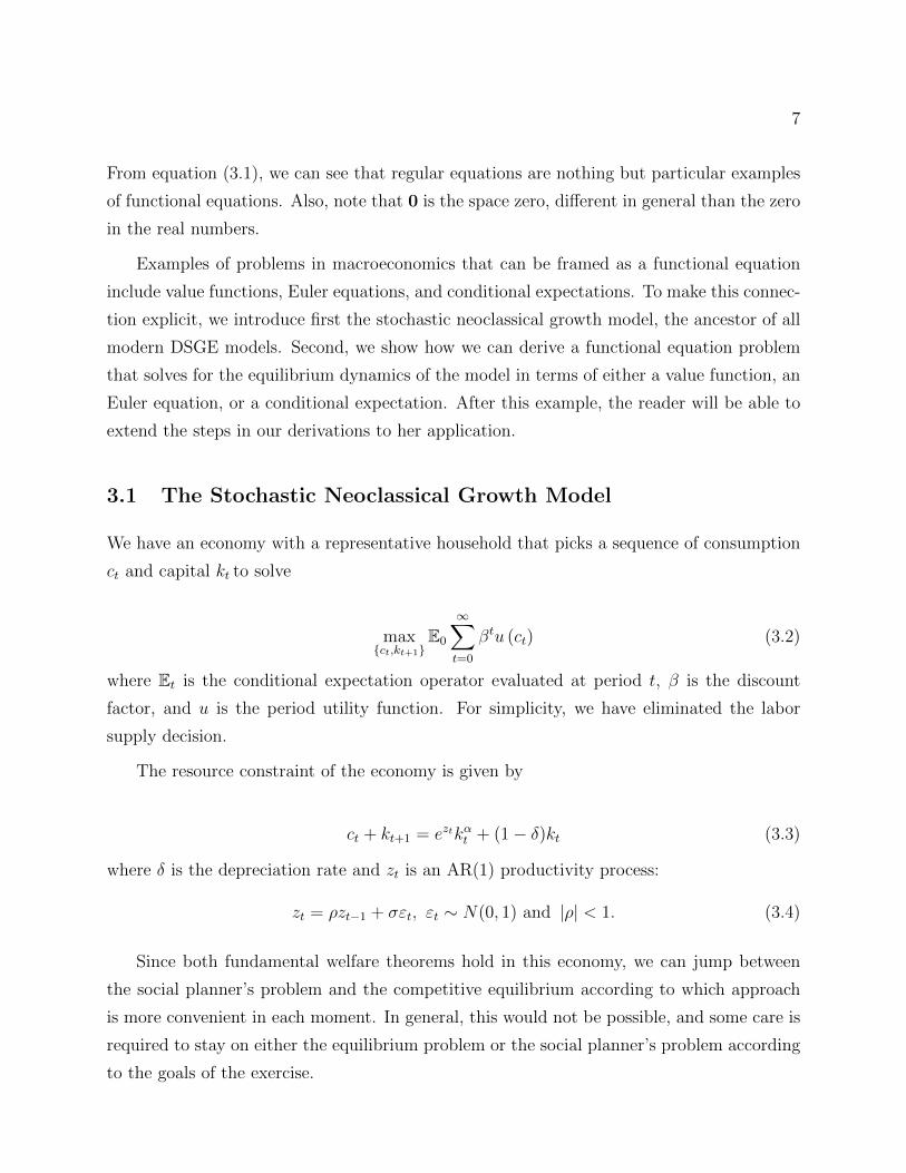
From equation (3.1), we can see that regular equations are nothing but particular examples

of functional equations. Also, note that 0 is the space zero, different in general than the zero

in the real numbers.

Examples of problems in macroeconomics that can be framed as a functional equation

include value functions, Euler equations, and conditional expectations. To make this connec-

tion explicit, we introduce first the stochastic neoclassical growth model, the ancestor of all

modern DSGE models. Second, we show how we can derive a functional equation problem

that solves for the equilibrium dynamics of the model in terms of either a value function, an

Euler equation, or a conditional expectation. After this example, the reader will be able to

extend the steps in our derivations to her application.

3.1 The Stochastic Neoclassical Growth Model

We have an economy with a representative household that picks a sequence of consumption

ct and capital kt to solve

maxct,kt+1

E0

∞∑t=0

βtu (ct) (3.2)

where Et is the conditional expectation operator evaluated at period t, β is the discount

factor, and u is the period utility function. For simplicity, we have eliminated the labor

supply decision.

The resource constraint of the economy is given by

ct + kt+1 = eztkαt + (1− δ)kt (3.3)

where δ is the depreciation rate and zt is an AR(1) productivity process:

zt = ρzt−1 + σεt, εt ∼ N(0, 1) and |ρ| < 1. (3.4)

Since both fundamental welfare theorems hold in this economy, we can jump between

the social planner’s problem and the competitive equilibrium according to which approach

is more convenient in each moment. In general, this would not be possible, and some care is

required to stay on either the equilibrium problem or the social planner’s problem according

to the goals of the exercise.

8

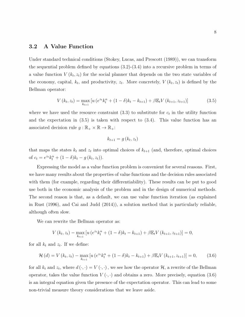
3.2 A Value Function

Under standard technical conditions (Stokey, Lucas, and Prescott (1989)), we can transform

the sequential problem defined by equations (3.2)-(3.4) into a recursive problem in terms of

a value function V (kt, zt) for the social planner that depends on the two state variables of

the economy, capital, kt, and productivity, zt. More concretely, V (kt, zt) is defined by the

Bellman operator:

V (kt, zt) = maxkt+1

[u (eztkαt + (1− δ)kt − kt+1) + βEtV (kt+1, zt+1)] (3.5)

where we have used the resource constraint (3.3) to substitute for ct in the utility function

and the expectation in (3.5) is taken with respect to (3.4). This value function has an

associated decision rule g : R+ × R→ R+:

kt+1 = g (kt, zt)

that maps the states kt and zt into optimal choices of kt+1 (and, therefore, optimal choices

of ct = eztkαt + (1− δ)kt − g (kt, zt)).

Expressing the model as a value function problem is convenient for several reasons. First,

we have many results about the properties of value functions and the decision rules associated

with them (for example, regarding their differentiability). These results can be put to good

use both in the economic analysis of the problem and in the design of numerical methods.

The second reason is that, as a default, we can use value function iteration (as explained

in Rust (1996), and Cai and Judd (2014)), a solution method that is particularly reliable,

although often slow.

We can rewrite the Bellman operator as:

V (kt, zt)−maxkt+1

[u (eztkαt + (1− δ)kt − kt+1) + βEtV (kt+1, zt+1)] = 0,

for all kt and zt. If we define:

H (d) = V (kt, zt)−maxkt+1

[u (eztkαt + (1− δ)kt − kt+1) + βEtV (kt+1, zt+1)] = 0, (3.6)

for all kt and zt, where d (·, ·) = V (·, ·) , we see how the operator H, a rewrite of the Bellman

operator, takes the value function V (·, ·) and obtains a zero. More precisely, equation (3.6)

is an integral equation given the presence of the expectation operator. This can lead to some

non-trivial measure theory considerations that we leave aside.

9

3.3 Euler Equation

We have outlined several reasons why casting the problem in terms of a value function is

attractive. Unfortunately, this formulation can be difficult. If the model does not satisfy

the two fundamental welfare theorems, we cannot easily move between the social planner’s

problem and the competitive equilibrium. In that case, also, the value function of the

household and firms will require laws of motion for individual and aggregate state variables

that can be challenging to characterize.2

An alternative is to work directly with the set of equilibrium conditions of the model.

These include the first-order conditions for households, firms, and, if specified, government,

budget and resource constraints, market clearing conditions, and laws of motion for exoge-

nous processes. Since, at the core of these equilibrium conditions, we will have the Euler

equations for the agents in the model that encode optimal behavior (with the other condi-

tions being somewhat mechanical), this approach is commonly known as the Euler equation

method (sometimes also referred to as solving the equilibrium conditions of the models).

This solution strategy is extremely general and it allows us to handle non-Pareto efficient

economies without further complications.

In the case of the stochastic neoclassical growth model, the Euler equation for the se-

quential problem defined by equations (3.2)-(3.4) is:

u′ (ct) = βEt[u′ (ct+1)

(αezt+1kα−1

t+1 + 1− δ)]. (3.7)

Again, under standard technical conditions, there is a decision rule g : R+×R→ R2+ for the

social planner that gives the optimal choice of consumption (g1 (kt, zt)) and capital tomorrow

(g2 (kt, zt)) given capital, kt, and productivity, zt, today. Then, we can rewrite the first-order

condition as:

u′(g1 (kt, zt)

)= βEt

[u′(g1(g2 (kt, zt) , zt+1

)) (αeρzt+σεt+1

(g2 (kt, zt)

)α−1+ 1− δ

)],

for all kt and zt, where we have used the law of motion for productivity (3.4) to substitute

forzt+1 or, alternatively: u′ (g1 (kt, zt))

−βEt[u′ (g1 (g2 (kt, zt) , zt+1))

(αeρzt+σεt+1 (g2 (kt, zt))

α−1+ 1− δ

)] = 0, (3.8)

2See Hansen and Prescott (1995), for examples of how to recast a non-Pareto optimal economy into the

mold of an associated Pareto-optimal problem.

10

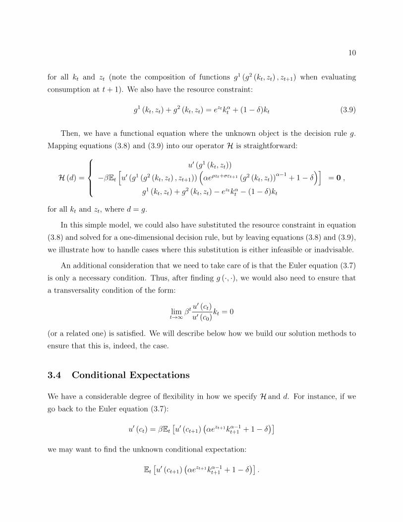
for all kt and zt (note the composition of functions g1 (g2 (kt, zt) , zt+1) when evaluating

consumption at t+ 1). We also have the resource constraint:

g1 (kt, zt) + g2 (kt, zt) = eztkαt + (1− δ)kt (3.9)

Then, we have a functional equation where the unknown object is the decision rule g.

Mapping equations (3.8) and (3.9) into our operator H is straightforward:

H (d) =

u′ (g1 (kt, zt))

−βEt[u′ (g1 (g2 (kt, zt) , zt+1))

(αeρzt+σεt+1 (g2 (kt, zt))

α−1+ 1− δ

)]g1 (kt, zt) + g2 (kt, zt)− eztkαt − (1− δ)kt

= 0 ,

for all kt and zt, where d = g.

In this simple model, we could also have substituted the resource constraint in equation

(3.8) and solved for a one-dimensional decision rule, but by leaving equations (3.8) and (3.9),

we illustrate how to handle cases where this substitution is either infeasible or inadvisable.

An additional consideration that we need to take care of is that the Euler equation (3.7)

is only a necessary condition. Thus, after finding g (·, ·), we would also need to ensure that

a transversality condition of the form:

limt→∞

βtu′ (ct)

u′ (c0)kt = 0

(or a related one) is satisfied. We will describe below how we build our solution methods to

ensure that this is, indeed, the case.

3.4 Conditional Expectations

We have a considerable degree of flexibility in how we specify H and d. For instance, if we

go back to the Euler equation (3.7):

u′ (ct) = βEt[u′ (ct+1)

(αezt+1kα−1

t+1 + 1− δ)]

we may want to find the unknown conditional expectation:

Et[u′ (ct+1)

(αezt+1kα−1

t+1 + 1− δ)].

11

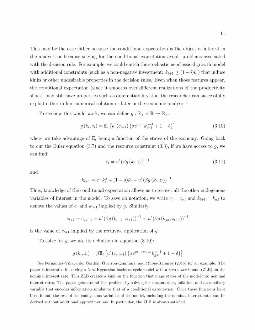
This may be the case either because the conditional expectation is the object of interest in

the analysis or because solving for the conditional expectation avoids problems associated

with the decision rule. For example, we could enrich the stochastic neoclassical growth model

with additional constraints (such as a non-negative investment: kt+1 ≥ (1−δ)kt) that induce

kinks or other undesirable properties in the decision rules. Even when those features appear,

the conditional expectation (since it smooths over different realizations of the productivity

shock) may still have properties such as differentiability that the researcher can successfully

exploit either in her numerical solution or later in the economic analysis.3

To see how this would work, we can define g : R+ × R→ R+:

g (kt, zt) = Et[u′ (ct+1)

(αezt+1kα−1

t+1 + 1− δ)]

(3.10)

where we take advantage of Et being a function of the states of the economy. Going back

to our the Euler equation (3.7) and the resource constraint (3.3), if we have access to g, we

can find:

ct = u′ (βg (kt, zt))−1 (3.11)

and

kt+1 = eztkαt + (1− δ)kt − u′ (βg (kt, zt))−1 .

Thus, knowledge of the conditional expectation allows us to recover all the other endogenous

variables of interest in the model. To save on notation, we write ct = cg,t and kt+1 = kg,t to

denote the values of ct and kt+1 implied by g. Similarly:

ct+1 = cg,t+1 = u′ (βg (kt+1, zt+1))−1 = u′ (βg (kg,t, zt+1))−1

is the value of ct+1 implied by the recursive application of g.

To solve for g, we use its definition in equation (3.10):

g (kt, zt) = βEt[u′ (cg,t+1)

(αeρzt+σεt+1kα−1

g,t + 1− δ)]

3See Fernandez-Villaverde, Gordon, Guerron-Quintana, and Rubio-Ramırez (2015) for an example. The

paper is interested in solving a New Keynesian business cycle model with a zero lower bound (ZLB) on the

nominal interest rate. This ZLB creates a kink on the function that maps states of the model into nominal

interest rates. The paper gets around this problem by solving for consumption, inflation, and an auxiliary

variable that encodes information similar to that of a conditional expectation. Once these functions have

been found, the rest of the endogenous variables of the model, including the nominal interest rate, can be

derived without additional approximations. In particular, the ZLB is always satisfied.

12

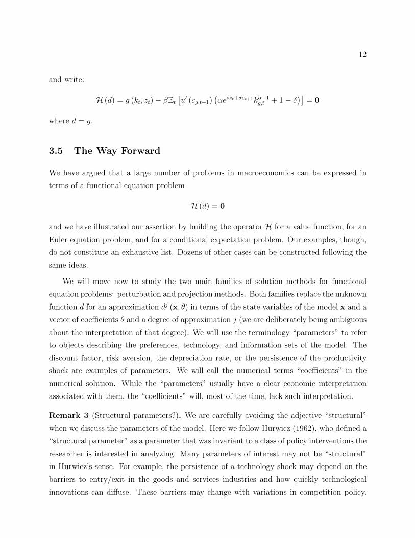
and write:

H (d) = g (kt, zt)− βEt[u′ (cg,t+1)

(αeρzt+σεt+1kα−1

g,t + 1− δ)]

= 0

where d = g.

3.5 The Way Forward

We have argued that a large number of problems in macroeconomics can be expressed in

terms of a functional equation problem

H (d) = 0

and we have illustrated our assertion by building the operator H for a value function, for an

Euler equation problem, and for a conditional expectation problem. Our examples, though,

do not constitute an exhaustive list. Dozens of other cases can be constructed following the

same ideas.

We will move now to study the two main families of solution methods for functional

equation problems: perturbation and projection methods. Both families replace the unknown

function d for an approximation dj (x, θ) in terms of the state variables of the model x and a

vector of coefficients θ and a degree of approximation j (we are deliberately being ambiguous

about the interpretation of that degree). We will use the terminology “parameters” to refer

to objects describing the preferences, technology, and information sets of the model. The

discount factor, risk aversion, the depreciation rate, or the persistence of the productivity

shock are examples of parameters. We will call the numerical terms “coefficients” in the

numerical solution. While the “parameters” usually have a clear economic interpretation

associated with them, the “coefficients” will, most of the time, lack such interpretation.

Remark 3 (Structural parameters?). We are carefully avoiding the adjective “structural”

when we discuss the parameters of the model. Here we follow Hurwicz (1962), who defined a

“structural parameter” as a parameter that was invariant to a class of policy interventions the

researcher is interested in analyzing. Many parameters of interest may not be “structural”

in Hurwicz’s sense. For example, the persistence of a technology shock may depend on the

barriers to entry/exit in the goods and services industries and how quickly technological

innovations can diffuse. These barriers may change with variations in competition policy.

13

See a more detailed discussion on the “structural” character of parameters in DSGE models

as well as empirical evidence in Fernandez-Villaverde and Rubio-Ramırez (2008).

The states of the model will be determined by the structure of the model. Even if, in

the words of Thomas Sargent, “finding the states is an art” (meaning both that there is no

constructive algorithm to do so and that the researcher may be able to find different sets of

states that accomplish the goal of fully describing the situation of the model, some of which

may be more useful than the others in one context but less so in another one), determining

the states is a step previous to the numerical solution of the model and, therefore, outside

the purview of this chapter.

4 Perturbation

Perturbation methods build approximate solutions to a DSGE economy by starting from the

exact solution of a particular case of the model or from the solution of a nearby model whose

solution we have access to. Perturbation methods are also known as asymptotic methods,

although we will avoid such a name because it risks confusion with related techniques re-

garding the large sample properties of estimators as the ones we will introduce in Part II of

the chapter. In their more common incarnation in macroeconomics, perturbation algorithms

build Taylor series approximations to the solution of a DSGE model around its determinis-

tic steady state using implicit-function theorems. However, other perturbation approaches

are possible, and we should always talk about a perturbation of the model instead of the

perturbation. With a long tradition in physics and other natural sciences, perturbation the-

ory was popularized in economics by Judd and Guu (1993) and it has been authoritatively

presented by Judd (1998), Judd and Guu (2001), and Jin and Judd (2002).4 Since there

is much relevant material about perturbation problems in economics (including a formal

mathematical background regarding solvability conditions, and more advanced perturbation

techniques such as gauges and Pade approximants) that we cannot cover in this chapter, we

refer the interested reader to these sources.

4Perturbation approaches were already widely used in physics in the 19th century. They became a central

tool in the natural sciences with the development of quantum mechanics in the first half of the 20th century.

Good general references on perturbation methods are Simmonds and Mann (1997) and Bender and Orszag

(1999).

14

Over the last two decades, perturbation methods have gained much popularity among

researchers for four reasons. First, perturbation solutions are accurate around an approxi-

mation point. Perturbation methods find an approximate solution that is inherently local.

In other words, the approximated solution is extremely close to the exact, yet unknown,

solution around the point where we take the Taylor series expansion. However, researchers

have documented that perturbation often displays good global properties along a wide range

of state variable values. See the evidence in Judd (1998), Aruoba, Fernandez-Villaverde, and

Rubio-Ramırez (2006) and Caldara, Fernandez-Villaverde, Rubio-Ramırez, and Yao (2012).

Also, as we will discuss below, the perturbed solution can be employed as an input for global

solution methods, such as value function iteration. Second, the structure of the approximate

solution is intuitive and easily interpretable. For example, a second-order expansion of a

DSGE model includes a term that corrects for the standard deviation of the shocks that

drive the stochastic dynamics of the economy. This term, which captures precautionary be-

havior, breaks the certainty equivalence of linear approximations that makes the discussion

of welfare and risk in a linearized world challenging. Third, as we will explain below, a tradi-

tional linearization is nothing but a first-order perturbation. Hence, economists can import

into perturbation theory much of their knowledge and practical experience while, simultane-

ously, being able to incorporate the formal results developed in applied mathematics. Fourth,

thanks to open-source software such as Dynare and Dynare++ (developed by Stephane Ad-

jemian, Michel Juillard, and their team of collaborators), higher-order perturbations are easy

to compute even for practitioners less familiar with numerical methods.5

4.1 The Framework

Perturbation methods solve the functional equation problem:

H (d) = 0

by specifying a Taylor series expansion to the unknown function d : Ω→ Rm in terms of the

n state variables of the model x and some coefficients θ. For example, a second-order Taylor

5Dynare (a toolbox for Matlab) and Dynare++ (a stand-alone application) allow the researcher to write, in

a concise and transparent language, the equilibrium conditions of a DSGE model and find a perturbation solu-

tion to it, up to the third order in Dynare and an arbitrary order in Dynare++. See http://www.dynare.org/.

15

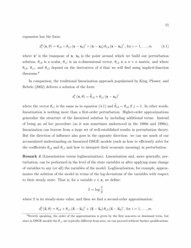
expansion has the form:

d2i (x, θ) = θi,0 + θi,1 (x− x0)′ + (x− x0) θi,2 (x− x0)′ , for i = 1, . . . ,m (4.1)

where x′ is the transpose of x, x0 is the point around which we build our perturbation

solution, θi,0 is a scalar, θi,1 is an n-dimensional vector, θi,2 is a n × n matrix, and where

θi,0, θi,1, and θi,2 depend on the derivatives of d that we will find using implicit-function

theorems.6

In comparison, the traditional linearization approach popularized by King, Plosser, and

Rebelo (2002) delivers a solution of the form:

d1i (x, θ) = θi,0 + θi,1 (x− x0)′

where the vector θi,1 is the same as in equation (4.1) and θi,0 = θi,0 if j = 1. In other words,

linearization is nothing more than a first-order perturbation. Higher-order approximations

generalize the structure of the linearized solution by including additional terms. Instead

of being an ad hoc procedure (as it was sometimes understood in the 1980s and 1990s),

linearization can borrow from a large set of well-established results in perturbation theory.

But the direction of influence also goes in the opposite direction: we can use much of our

accumulated understanding on linearized DSGE models (such as how to efficiently solve for

the coefficients θi,0 and θi,1 and how to interpret their economic meaning) in perturbation.

Remark 4 (Linearization versus loglinearization). Linearization and, more generally, per-

turbation, can be performed in the level of the state variables or after applying some change

of variables to any (or all) the variables of the model. Loglinearization, for example, approx-

imates the solution of the model in terms of the log-deviations of the variables with respect

to their steady state. That is, for a variable x ∈ x, we define:

x = logx

x

where x is its steady-state value, and then we find a second-order approximation:

d2i (x, θ) = θi,0 + θi,1 (x− x0)′ + (x− x0) θi,2 (x− x0)′ , for i = 1, . . . ,m.

6Strictly speaking, the order of the approximation is given by the first non-zero or dominant term, but

since in DSGE models the θi,1 are typically different from zero, we can proceed without further qualifications.

16

If x0 is the deterministic steady state (this is more often than not the case), x0 = 0, since

for all variables x ∈ x

x0 = logx

x= 0.

This result provides a compact representation:

d2i (x, θ) = θi,0 + θi,1x

′ + xθi,2x′, for i = 1, . . . ,m.

Loglinear solutions are easy to read (the loglinear deviation is an approximation of the

percentage deviation with respect to the steady state) and, in some circumstances, they can

improve the accuracy of the solution. We will revisit the change of variables later in the

chapter.

Before getting into technical details of how to implement perturbation methods, we will

briefly distinguish between regular and singular perturbations. A regular perturbation is a

situation where a small change in the problem induces a small change in the solution. An

example is a standard New Keynesian model (Woodford (2003)). A small change in the

standard deviation of the monetary policy shock will lead to a small change in the properties

of the equilibrium dynamics (i.e., the standard deviation and autocorrelation of variables

such as output or inflation). A singular perturbation is a situation where a small change in

the problem induces a large change in the solution. An example can be an excess demand

function. A small change in the excess demand function may lead to an arbitrarily large

change in the price that clears the market.

Many problems involving DSGE models will result in regular perturbations. Thus, we

will concentrate on them. But this is not necessarily the case. For instance, introducing a new

asset in an incomplete market model can lead to large changes in the solution. As researchers

pay more attention to models with financial frictions and/or market incompleteness, this class

of problems may become common. Researchers will need to learn more about how to apply

singular perturbations. See, for pioneering work, Judd and Guu (1993), and a presentation

of bifurcation methods for singular problems in Judd (1998).

4.2 The General Case

We are now ready to deal with the details of how to implement a perturbation. We present

first the general case of how to find a perturbation solution of a DSGE model by 1) using

17

the equilibrium conditions of the model and 2) by finding a higher-order Taylor series ap-

proximation. Once we have mastered this task, it would be straightforward to extend the

results to other problems, such as the solution of a value function, and to conceive other

possible perturbation schemes. This subsection follows much of the structure and notation

of Section 3 in Schmitt-Grohe and Uribe (2004).

We start by writing the equilibrium conditions of the model as

EtH(y,y′,x,x′) = 0, (4.2)

where y is an ny× 1 vector of controls, x is an nx× 1 vector of states, and n = nx +ny. The

operatorH : Rny×Rny×Rnx×Rnx → Rn stacks all the equilibrium conditions, some of which

will have expectational terms, some of which will not. Without loss of generality, and with

a slight change of notation with respect to Section 3, we place the conditional expectation

operator outside H: for those equilibrium conditions without expectations, the conditional

expectation operator will not have any impact. Moving Et outside H will make some of the

derivations below easier to follow. Also, to save on space, when there is no ambiguity, we

will employ the recursive notation where x represents a variable at period t and x′ a variable

at period t+ 1.

It will also be convenient to separate the endogenous state variables (capital, asset posi-

tions, etc.) from the exogenous state variables (productivity shocks, preference shocks, etc.).

In that way, it will be easier to see the variables on which the perturbation parameter that

we will introduce below will have a direct effect. Thus, we partition the state vector x (and

taking transposes) as

x = [x′1; x′2]′.

where x1 is an (nx − nε)× 1 vector of endogenous state variables and x2 is an nε × 1 vector

of exogenous state variables.

4.2.1 Steady State

If we suppress the stochastic component of the model (more details below), we can define

the deterministic steady-state of the model as vectors (x,y) such that:

H(y, y, x, x) = 0. (4.3)

18

The solution (x,y) of this problem can often be found analytically. When this cannot be

done, it is possible to resort to a standard non-linear equation solver.

The previous paragraph glossed over the possibility that the model we are dealing with

either does not have a steady state or that it has several of them (in fact, we can even have

a continuum of steady states). Given our level of abstraction with the definition of equation

(4.2), we cannot rule out any of these possibilities. Galor (2007) discusses in detail the

existence and stability (local and global) of steady states in discrete time dynamic models.

A case of interest is when the model, instead of having a steady state, has a balanced

growth path (BGP): that is, when the variables of the model (with possibly some exceptions

such as labor) grow at the same rate (either deterministic or stochastic). Given that per-

turbation is an inherently local solution method, we cannot deal directly with solving such

a model. However, on many occasions, we can rescale the variables xt in the model by the

trend µt:

xt =xtµt

to render them stationary (the trend itself may be a complicated function of some tech-

nological processes in the economy, as when we have both neutral and investment-specific

technological change; see Fernandez-Villaverde and Rubio-Ramırez (2007)). Then, we can

undertake the perturbation in the rescaled variable xt and undo the rescaling when using

the approximated solution for analysis and simulation.7

Remark 5 (Simplifying the solution of (x,y)). Finding the solution (x,y) can often be

made much easier by using two “tricks.” One is to substitute some of the variables away

from the operator H (·) and reduce the system from being one of n equations in n unknowns

into a system of n′ < n equations in n′ unknowns. For example, if we have a law of motion

for capital involving capital next period, capital next period, and investment:

kt+1 = (1− δ) kt + it

we can substitute out investment throughout the whole system just by writing:

it = kt+1 − (1− δ) kt.7This rescaling is also useful with projection methods since they need a bounded domain of the state

variables.

19

Since the complexity of solving a non-linear system of equations grows exponentially in the

dimension of the problem (see Sikorski (1985), for classic results on computational complex-

ity), even a few substitutions can produce considerable improvements.

A second possibility is to select parameter values to pin down one or more variables of

the model and then to solve all the other variables as a function of the fixed variables. To

illustrate this point, let us consider a simple stochastic neoclassical growth model with a

representative household with utility function:

E0

∞∑t=0

βt(

log ct − ψl1+ηt

1 + η

)where the notation is the same as in Section 3 and a production function:

outputt = Atkαt l

1−αt

where At is the productivity level and a law of motion for capital:

kt+1 = outputt + (1− δ)kt − ct.

This model has a static optimality condition for labor supply of the form:

ψctlηt = wt

where wt is the wage. Since with the log-CRRA utility function that we selected lt does not

have a natural unit, we can fix its deterministic steady-state value, for example, l = 1. This

normalization is as good as any other and the researcher can pick the normalization that

best suits her needs.

Then, we can analytically solve the rest of the equilibrium conditions of the model for

all other endogenous variables as a function of l = 1. After doing so, we return to the static

optimality condition to obtain the value of the parameter ψ as:

ψ =w

clη =

w

c

where c and w are the deterministic steady-state values of consumption and wage, respec-

tively. An alternative way to think about this procedure is to realize that it is often easier

to find parameter values that imply a particular endogenous variable value than to solve for

those endogenous variable values as a function of an arbitrary parameter value.

20

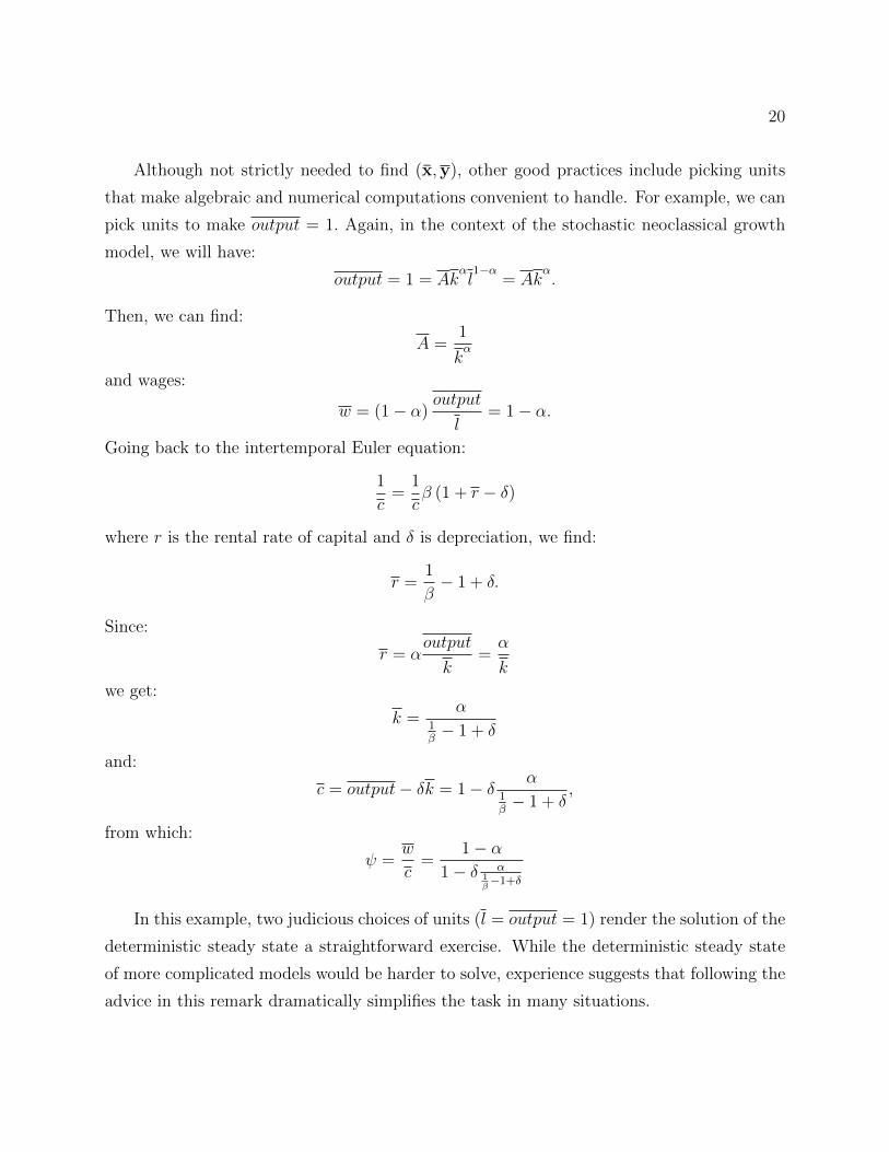
Although not strictly needed to find (x,y), other good practices include picking units

that make algebraic and numerical computations convenient to handle. For example, we can

pick units to make output = 1. Again, in the context of the stochastic neoclassical growth

model, we will have:

output = 1 = Akαl1−α

= Akα.

Then, we can find:

A =1

kα

and wages:

w = (1− α)output

l= 1− α.

Going back to the intertemporal Euler equation:

1

c=

1

cβ (1 + r − δ)

where r is the rental rate of capital and δ is depreciation, we find:

r =1

β− 1 + δ.

Since:

r = αoutput

k=α

k

we get:

k =α

1β− 1 + δ

and:

c = output− δk = 1− δ α1β− 1 + δ

,

from which:

ψ =w

c=

1− α1− δ α

1β−1+δ

In this example, two judicious choices of units (l = output = 1) render the solution of the

deterministic steady state a straightforward exercise. While the deterministic steady state

of more complicated models would be harder to solve, experience suggests that following the

advice in this remark dramatically simplifies the task in many situations.

21

The deterministic steady state (x,y) is different from a fixed point (x, y) of (4.2):

EtH(y, y, x, x) = 0,

because in the former case we eliminate the conditional expectation operator while in the

latter we do not. The vector (x, y) is sometimes known as the stochastic steady state

(although, since we find the idea of mixing the words “stochastic” and “steady state” in the

same term confusing, we will avoid that terminology).

4.2.2 Exogenous Stochastic Process

For the exogenous stochastic variables, we specify a stochastic process of the form:

x′2 = C(x2) + σηεε′ (4.4)

where C is a potentially non-linear function. At our current level of abstraction, we are

not imposing much structure on C, but in concrete applications, we will need to add more

constraints. For example, researchers often assume that all the eigenvalues of the Hessian

matrix of C evaluated at the steady state (x,y) lie within the unit circle. The vector

ε′ contains the nε exogenous zero-mean innovations. Initially, we only assume that ε′ is

independent and identically distributed with finite second moments, meaning that we do

not rely on any distributional assumption. Thus, the innovations may be non-Gaussian.

This is denoted by ε′ ∼ iid (0, I). Additional moment restrictions will be introduced as

needed in each concrete application. Finally, ηε is an nε × nε matrix that determines the

variances-covariances of the innovations, and σ ≥ 0 is a perturbation parameter that scales

η.

Often, it will be the case that C is linear:

x′2 = Cx2 + σηεε′

where C is an nε × nε matrix, with all its eigenvalues with modulus less than one.

Remark 6 (Linearity of innovations). The assumption that innovations enter linearly in

equation (4.4) may appear restrictive, but it is without loss of generality. Imagine that

instead of equation (4.4), we have:

x2,t = D(x2,t−1, σηεεt).

22

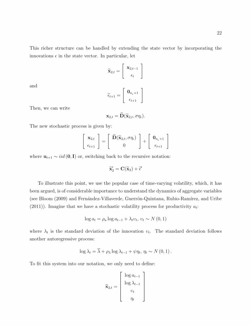
This richer structure can be handled by extending the state vector by incorporating the

innovations ε in the state vector. In particular, let

x2,t =

[x2,t−1

εt

]

and

εt+1 =

[0nε×1

εt+1

]Then, we can write

x2,t = D(x2,t, σηε).

The new stochastic process is given by:[x2,t

εt+1

]=

[D(x2,t, σηε)

0

]+

[0nε×1

εt+1

]

where ut+1 ∼ iid (0, I) or, switching back to the recursive notation:

x′2 = C(x2) + ε′

To illustrate this point, we use the popular case of time-varying volatility, which, it has

been argued, is of considerable importance to understand the dynamics of aggregate variables

(see Bloom (2009) and Fernandez-Villaverde, Guerron-Quintana, Rubio-Ramırez, and Uribe

(2011)). Imagine that we have a stochastic volatility process for productivity at:

log at = ρa log at−1 + λtυt, υt ∼ N (0, 1)

where λt is the standard deviation of the innovation υt. The standard deviation follows

another autoregressive process:

log λt = λ+ ρλ log λt−1 + ψηt, ηt ∼ N (0, 1) .

To fit this system into our notation, we only need to define:

x2,t =

log at−1

log λt−1

υt

ηt

23

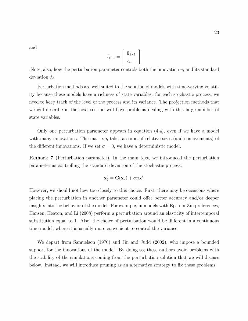
and

εt+1 =

[02×1

εt+1

].Note, also, how the perturbation parameter controls both the innovation υt and its standard

deviation λt.

Perturbation methods are well suited to the solution of models with time-varying volatil-

ity because these models have a richness of state variables: for each stochastic process, we

need to keep track of the level of the process and its variance. The projection methods that

we will describe in the next section will have problems dealing with this large number of

state variables.

Only one perturbation parameter appears in equation (4.4), even if we have a model

with many innovations. The matrix η takes account of relative sizes (and comovements) of

the different innovations. If we set σ = 0, we have a deterministic model.

Remark 7 (Perturbation parameter). In the main text, we introduced the perturbation

parameter as controlling the standard deviation of the stochastic process:

x′2 = C(x2) + σηεε′.

However, we should not hew too closely to this choice. First, there may be occasions where

placing the perturbation in another parameter could offer better accuracy and/or deeper

insights into the behavior of the model. For example, in models with Epstein-Zin preferences,

Hansen, Heaton, and Li (2008) perform a perturbation around an elasticity of intertemporal

substitution equal to 1. Also, the choice of perturbation would be different in a continuous

time model, where it is usually more convenient to control the variance.

We depart from Samuelson (1970) and Jin and Judd (2002), who impose a bounded

support for the innovations of the model. By doing so, these authors avoid problems with

the stability of the simulations coming from the perturbation solution that we will discuss

below. Instead, we will introduce pruning as an alternative strategy to fix these problems.

24

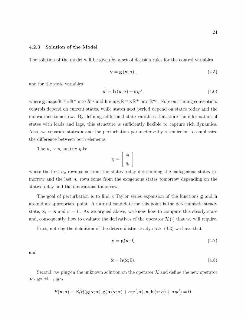
4.2.3 Solution of the Model

The solution of the model will be given by a set of decision rules for the control variables

y = g (x;σ) , (4.5)

and for the state variables

x′ = h (x;σ) + σηε′, (4.6)

where g maps Rnx×R+ into Rny and h maps Rnx×R+ into Rnx . Note our timing convention:

controls depend on current states, while states next period depend on states today and the

innovations tomorrow. By defining additional state variables that store the information of

states with leads and lags, this structure is sufficiently flexible to capture rich dynamics.

Also, we separate states x and the perturbation parameter σ by a semicolon to emphasize

the difference between both elements.

The nx × nε matrix η is:

η =

[∅ηε

]where the first nx rows come from the states today determining the endogenous states to-

morrow and the last nε rows come from the exogenous states tomorrow depending on the

states today and the innovations tomorrow.

The goal of perturbation is to find a Taylor series expansion of the functions g and h

around an appropriate point. A natural candidate for this point is the deterministic steady

state, xt = x and σ = 0. As we argued above, we know how to compute this steady state

and, consequently, how to evaluate the derivatives of the operator H (·) that we will require.

First, note by the definition of the deterministic steady state (4.3) we have that

y = g(x; 0) (4.7)

and

x = h(x; 0). (4.8)

Second, we plug-in the unknown solution on the operator H and define the new operator

F : Rnx+1 → Rn:

F (x;σ) ≡ EtH(g(x;σ),g(h (x;σ) + σηε′, σ),x,h (x;σ) + σηε′) = 0.

25

Since F (x;σ) = 0 for any values of x and σ, any derivatives of F must also be zero:

Fxki σj(x;σ) = 0, ∀x, σ, i, k, j,

where Fxki σj(x;σ) is the derivative of F with respect to the i-th component xi of x taken k

times and with respect to σ taken j times evaluated at (x;σ). Intuitively, the solution of

the model must satisfy the equilibrium conditions for all possible values of the states and σ.

Thus, any change in the values of the states or of σ must still keep the operator F exactly

at 0. We will exploit this important fact repeatedly.

Remark 8 (Existence of derivatives). We will assume, without further discussion, that all

the relevant derivatives of the operator F exist in a neighborhood of x. These differentiability

assumptions may be hard to check in concrete applications and more research in the area

would be welcomed (see the classic work of Santos (1992)). However, the components that

enter into F (utility functions, production functions, etc.) are usually smooth when we

deal with DSGE models, which suggest that the existence of these derivatives is a heroic

assumption (although the examples in Santos, 1993, are a cautionary sign). Judd (1998, p.

463) indicates, also, that if the derivative conditions were violated, our computations would

display telltale signs that would alert the researcher to the underlying problems.

The derivative assumption, however, traces the frontiers of problems suitable for pertur-

bation: if, for example, some variables are discrete or the relevant equilibrium conditions

are non-differentiable, perturbation cannot be applied. Two caveats about the previous

statement are, nevertheless, worthwhile to highlight. First, the presence of expectations of-

ten transforms problems that appear discrete into continuous ones. For example, deciding

whether or not to go to college can be “smoothed out” by a stochastic shock to college costs

or by an effort variable that controls how hard the prospective student is applying to college

or searching for funding. Second, even if the derivative assumption breaks down and the

perturbation solution is not valid, it may still be an excellent guess for another solution

method.

Remark 9 (Taking derivatives). The previous exposition demonstrates the central role of

derivatives in perturbation methods. Except for simple examples, manually calculating these

derivatives is too onerous. Thus, researchers need to rely on computers. A first possibility,

numerical derivatives, is inadvisable (Judd, 1998, chapter 7). The errors created by numerical

derivatives quickly accumulate and, after the second or third derivative, the perturbation

26

solution is too contaminated by them to be of any real use. A second possibility is to exploit

software that takes analytic derivatives, such as Mathematica or the symbolic toolbox of

Matlab. This route is usually straightforward, but it may slow down the computation and

require an inordinate amount of memory. A third final alternative is to employ automatic

differentiation, a technique that takes advantage of the application of the chain rule to a

series of elementary arithmetic operations and functions (for how automatic differentiation

can be applied to DSGE models, see Bastani and Guerrieri (2008)).

4.2.4 First-Order Perturbation

A first-order perturbation approximates g and h around (x;σ) = (x; 0) as:

g(x;σ) = g(x; 0) + gx(x; 0)(x− x)′ + gσ(x; 0)σ

h(x;σ) = h(x; 0) + hx(x; 0)(x− x)′ + hσ(x; 0)σ

where gx and hx are the gradients of g and h, respectively (including only the partial

derivatives with respect to components of x) and gσ and hσ the derivatives of g and h with

respect to the perturbation parameter σ.

Using equations (4.7) and (4.8), we can write

g(x;σ)− y = gx(x; 0)(x− x)′ + gσ(x; 0)σ

h(x;σ)− x = hx(x; 0)(x− x)′ + hσ(x; 0)σ.

Since we know (x,y), we only need to find gx(x; 0), gσ(x; 0), hx(x; 0), and hσ(x; 0) to

evaluate the approximation at any arbitrary point (x,σ). We are searching for n× (nx + 1)

coefficients (the nx × ny terms in gx(x; 0), the nx × nx terms in hx(x; 0), the ny terms in

gσ(x; 0), and the nx terms in hσ(x; 0)).

These coefficients can be found by using:

Fxi(x; 0) = 0, ∀i,

which gives us n× nx equations and

Fσ(x; 0) = 0,

which gives us n equations.

27

But before doing so, and to avoid runaway notation, we need to introduce the use of

tensors.

Remark 10 (Tensor notation). Tensor notation (or Einstein summation notation), com-

monly used in physics, keeps the algebra required to perform a perturbation at a manageable

level by eliminating∑

and ∂ signs. To further reduce clutter, the points of evaluation of a

derivative are skipped when they are unambiguous from context. An nth-rank tensor in an

m-dimensional space is an operator that has n indices and mn components and obeys certain

transformation rules. In our environment, [Hy]iα is the (i, α) element of the derivative of H

with respect to y:

1. The derivative of H with respect to y is an n× ny matrix.

2. Thus, [Hy]iα is the i-th row and α-th column element of this matrix.

3. When a subindex appears as a superindex in the next term, we are omitting a sum

operator. For example,

[Hy]iα[gx]

αβ [hx]

βj =

ny∑α=1

nx∑β=1

∂Hi

∂yα∂gα

∂xβ∂hβ

∂xj.

4. The generalization to higher derivatives is direct. If we have [Hy′y′ ]iαγ:

(a) Hy′y′ is a three-dimensional array with n rows, ny columns, and ny pages.

(b) Thus, [Hy′y′ ]iαγ denotes the i-th row, α-th column element, and γ-th page of this

matrix.

With the tensor notation, we can get into solving the system. First, gx(x; 0) and hx(x; 0)

are the solution to:

[Fx(x; 0)]ij = [Hy′ ]iα[gx]

αβ [hx]

βj + [Hy]

iα[gx]

αj + [Hx′ ]

iβ[hx]

βj + [Hx]

ij = 0; (4.9)

i = 1, . . . , n; j, β = 1, . . . , nx; α = 1, . . . , ny.

The derivatives of H evaluated at (y,y′,x,x′) = (y, y, x, x) are known. Therefore, we have

a system of n × nx quadratic equations in the n × nx unknowns given by the elements of

gx(x; 0) and hx(x; 0). After some algebra, the system (4.9) can be written as:

AP 2 −BP − C = 0

28

where the n× n matrix A involves terms from [Hy′ ]iα, the n× n matrix B terms from [Hy]

iα

and [Hx′ ]iβ, the n × n matrix C terms from [Hx]

ij and the n × n matrix P the terms [gx]

αβ

and [hx]βj (in our worked-out example of the next subsection we make this algebra explicit).

We can solve this system with a standard quadratic matrix equation solver.

Remark 11 (Quadratic equation solvers). The literature has proposed several procedures to

solve quadratic systems. Without being exhaustive, we can list Blanchard and Kahn (1980),

King and Watson (1998), Uhlig (1999), Klein (2000), and Sims (2002). These different

approaches vary in the details of how the solution to the system is found and how general

they are (regarding the regularity conditions they require). But, conditional on applicability,

all methods find the same policy functions since the linear space approximating a non-linear

space is unique.

For concision, we will only present one of the simplest of these procedures, as discussed

by Uhlig (1999, pp. 43-45). Given

AP 2 −BP − C = 0,

define the 2n× 2n matrix:

D =

[A 0n

0n In

]where In is the n×n identity matrix and 0n the n×n zero matrix, and the 2n× 2n matrix:

F =

[B C

In 0n

]

Let Q and Z be unitary matrices (i.e., QHQ = Y HY = I2n where H is the complex Hermitian

transposition operator). Let Φ and Σ be upper triangular matrices with diagonal elements

φii and σii. Then, we find the generalized Schur decomposition (QZ) of D and F :

Q′ΣZ = D

Q′ΦZ = F

such that the ratios of diagonal elements |φii/σii| are in increasing order (there exists a QZ

decomposition for every ordering of these ratios). In such a way, the stable (smaller than one)

generalized eigenvalues of F with respect to D would come first and the unstable generalized

eigenvalues (exceeding one and infinite) would come last. QZ decompositions are performed

29

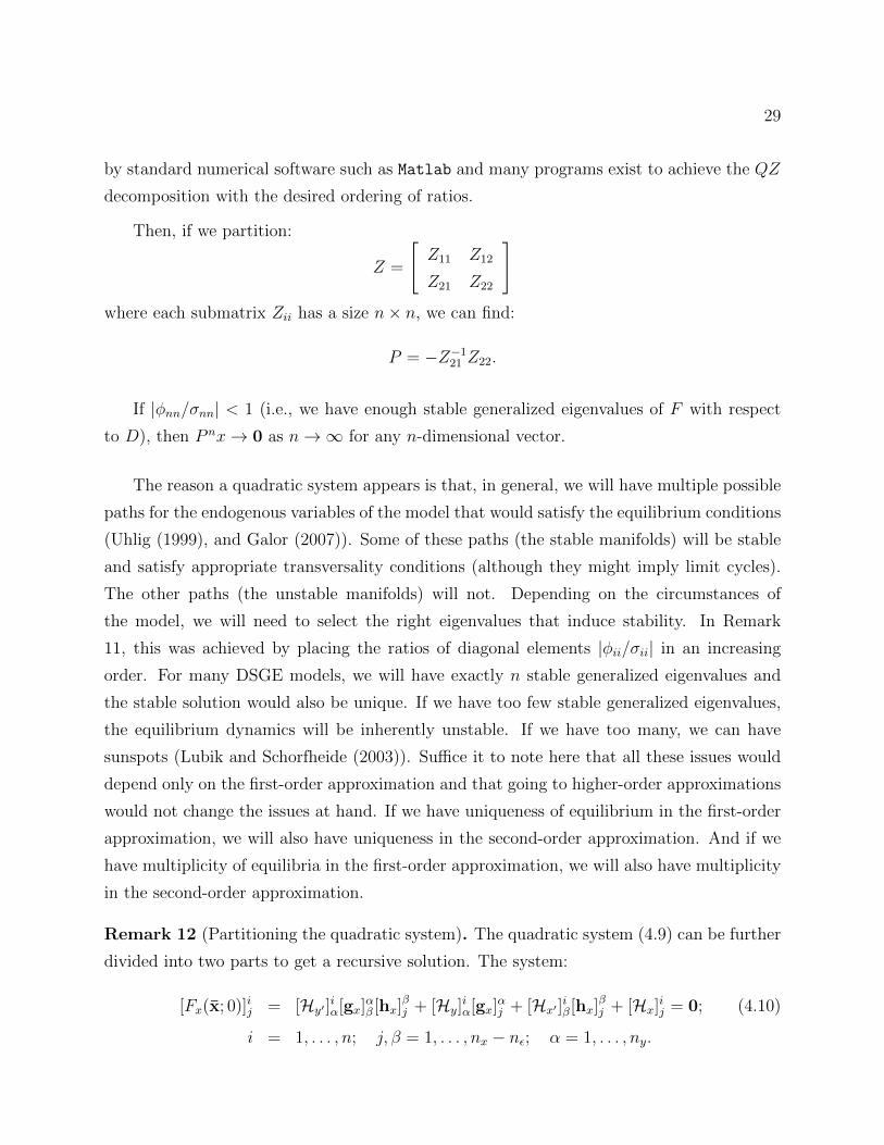
by standard numerical software such as Matlab and many programs exist to achieve the QZ

decomposition with the desired ordering of ratios.

Then, if we partition:

Z =

[Z11 Z12

Z21 Z22

]where each submatrix Zii has a size n× n, we can find:

P = −Z−121 Z22.

If |φnn/σnn| < 1 (i.e., we have enough stable generalized eigenvalues of F with respect

to D), then P nx→ 0 as n→∞ for any n-dimensional vector.

The reason a quadratic system appears is that, in general, we will have multiple possible

paths for the endogenous variables of the model that would satisfy the equilibrium conditions

(Uhlig (1999), and Galor (2007)). Some of these paths (the stable manifolds) will be stable

and satisfy appropriate transversality conditions (although they might imply limit cycles).

The other paths (the unstable manifolds) will not. Depending on the circumstances of

the model, we will need to select the right eigenvalues that induce stability. In Remark

11, this was achieved by placing the ratios of diagonal elements |φii/σii| in an increasing

order. For many DSGE models, we will have exactly n stable generalized eigenvalues and

the stable solution would also be unique. If we have too few stable generalized eigenvalues,

the equilibrium dynamics will be inherently unstable. If we have too many, we can have

sunspots (Lubik and Schorfheide (2003)). Suffice it to note here that all these issues would

depend only on the first-order approximation and that going to higher-order approximations

would not change the issues at hand. If we have uniqueness of equilibrium in the first-order

approximation, we will also have uniqueness in the second-order approximation. And if we

have multiplicity of equilibria in the first-order approximation, we will also have multiplicity

in the second-order approximation.

Remark 12 (Partitioning the quadratic system). The quadratic system (4.9) can be further

divided into two parts to get a recursive solution. The system:

[Fx(x; 0)]ij = [Hy′ ]iα[gx]

αβ [hx]

βj + [Hy]

iα[gx]

αj + [Hx′ ]

iβ[hx]

βj + [Hx]

ij = 0; (4.10)

i = 1, . . . , n; j, β = 1, . . . , nx − nε; α = 1, . . . , ny.

30

only involves the (nx − nε) × ny elements of gx(x; 0) and the (nx − nε) × nx elements of

hx(x; 0) related to the nx − nε endogenous state variables x1. Once we have solved the

(nx − nε)× (ny + nx) unknowns in this system, we can plug them into the system:

[Fx(x; 0)]ij = [Hy′ ]iα[gx]

αβ [hx]

βj + [Hy]

iα[gx]

αj + [Hx′ ]

iβ[hx]

βj + [Hx]

ij = 0; (4.11)

i = 1, . . . , n; j, β = nx − nε + 1, . . . , nx; α = 1, . . . , ny.

and solve for the nε × ny elements of gx(x; 0) and the nε × nx elements of hx((x; 0) related

to the nε stochastic variables x2.

This recursive solution has three advantages. The first, and most obvious, is that it

simplifies computations. The system (4.9) has nx × (ny + nx) unknowns, while the system

(4.10) has (nx − nε) × (ny + nx). The difference, nε × (ny + nx), makes the second system

considerably smaller. Think, for instance, about the medium-scale New Keynesian model in

Fernandez-Villaverde and Rubio-Ramırez (2008). In the notation of this chapter, the model

has nx = 20, ny = 1, and nε = 5. Thus, by partitioning the system, we go from solving for

420 unknowns to solve a first system of 315 unknowns and, later, a second system of 105

unknowns. The second advantage, which is not obvious in our compact notation, is that

system (4.11) is linear and, therefore, much faster to solve and with a unique solution. In

the next subsection, with our worked-out example, we will see this more clearly. The third

advantage is that, in some cases, we may only care about the coefficients associated with

the nx− nε endogenous state variables x1. This occurs, for example, when we are interested

in computing the deterministic transitional path of the model toward a steady state given

some initial conditions or when we are plotting impulse response functions generated by the

first-order approximation.

The coefficients gσ(x; 0) and hσ(x; 0) are the solution to the n equations:

[Fσ(x; 0)]i = Et[Hy′ ]iα[gx]

αβ [hσ]β + [Hy′ ]

iα[gx]

αβ [η]βφ[ε′]φ + [Hy′ ]

iα[gσ]α

+[Hy]iα[gσ]α + [Hx′ ]

iβ[hσ]β + [Hx′ ]

iβ[η]βφ[ε′]φ

i = 1, . . . , n; α = 1, . . . , ny; β = 1, . . . , nx; φ = 1, . . . , nε.

Then:

[Fσ(x; 0)]i = [Hy′ ]iα[gx]

αβ [hσ]β + [Hy′ ]

iα[gσ]α + [Hy]

iα[gσ]α + [fx′ ]

iβ[hσ]β = 0;

i = 1, . . . , n; α = 1, . . . , ny; β = 1, . . . , nx; φ = 1, . . . , nε.

31

Inspection of the previous equations shows that they are linear and homogeneous equa-

tions in gσ and hσ. Thus, if a unique solution exists, it satisfies:

gσ = 0

hσ = 0

In other words, the coefficients associated with the perturbation parameter are zero and the

first-order approximation is

g(x;σ)− y = gx(x; 0)(x− x)′

h(x;σ)− x = hx(x; 0)(x− x)′.

These equations embody certainty equivalence as defined by Simon (1956) and Theil (1957).

Under certainty equivalence, the solution of the model, up to first-order, is identical to the

solution of the same model under perfect foresight (or under the assumption that σ = 0).

Certainty equivalence does not preclude the realization of the shock from appearing in the

decision rule. What certainty equivalence precludes is that the standard deviation of it

appears as an argument by itself, regardless of the realization of the shock.

The intuition for the presence of certainty equivalence is simple. Risk-aversion depends

on the second derivative of the utility function (concave utility). However, Leland (1968)

and Sandmo (1970) showed that precautionary behavior depends on the third derivative of

the utility function. But a first-order perturbation involves the equilibrium conditions of

the model (which includes first derivatives of the utility function, for example, in the Euler

equation that equates marginal utilities over time) and first derivatives of these equilibrium

conditions (and, therefore, second derivatives of the utility function), but not higher-order

derivatives.

Certainty equivalence has several drawbacks. First, it makes it difficult to talk about

the welfare effects of uncertainty. Although the dynamics of the model are still partially

driven by the variance of the innovations (the realizations of the innovations depend on

it), the agents in the model do not take any precautionary behavior to protect themselves

from that variance, biasing any welfare computation. Second, related to the first point, the

approximated solution generated under certainty equivalence cannot generate any risk pre-

mia for assets, a strongly counterfactual prediction.8 Third, certainty equivalence prevents

8In general equilibrium, there is an intimate link between welfare computations and asset pricing. An

exercise on the former is always implicitly an exercise on the latter (see Alvarez and Jermann (2004)).

32

researchers from analyzing the consequences of changes in volatility.

Remark 13 (Perturbation and LQ approximations). Kydland and Prescott (1982) -and

many papers after them- took a different route to solving DSGE models. Imagine that

we have an optimal control problem that depends on nx states xt and nu control variables

ut. To save on notation, let us also define the column vector wt = [xt,ut]′ of dimension

nw = nx + nu. Then, we can write the optimal control problem as:

maxE0

∞∑t=0

βtr (wt)

s.t. xt+1 = A (wt, εt)

where r is a return function, εt a vector of nε innovations with zero mean and finite variance,

and A summarizes all the constraints and laws of motion of the economy. By appropriately

enlarging the state space, this notation can accommodate the innovations having an impact

on the period return function and some variables being both controls and states.

In the case where the return function r is quadratic, i.e.

r (wt) = B0 +B1wt + w′tQwt

(where B0 is a constant, B1 a row vector 1 × nw, and B2 is an nw × nw matrix) and the

function A is linear:

xt+1 = B3wt +B4εt

(where B3 is an nx × nw matrix and B4 is an nx × nε matrix), we are facing a stochastic

discounted linear-quadratic regulator (LQR) problem. There is a large and well-developed

research area on LQR problems. This literature is summarized by Anderson, Hansen, Mc-

Grattan, and Sargent (1996) and Hansen and Sargent (2013). In particular, we know that

the optimal decision rule in this environment is a linear function of the states and the inno-

vations:

ut = Fwwt + Fεεt

where Fw can be found by solving a Ricatti equation (Anderson, Hansen, McGrattan, and

Sargent, 1996, pp. 182-183) and Fε by solving a Sylvester equation (Anderson, Hansen,

McGrattan, and Sargent, 1996, pp. 202-205). Interestingly, Fw is independent of the variance

of εt. That is, if εt has a zero variance, then the optimal decision rule is simply:

ut = Fwwt.

33

This neat separation between the computation of Fw and of Fε allows the researcher to deal

with large problems with ease. However, it also implies certainty equivalence.

Kydland and Prescott (1982) set up the social planner’s problem of their economy, which

fits into an optimal regulator problem, and they were able to write a function A that was

linear in wt, but they did not have a quadratic return function. Instead, they took a

quadratic approximation to the objective function of the social planner. Most of the literature

that followed them used a Taylor series approximation of the objective function around the

deterministic steady state, sometimes called the approximated LQR problem (Kydland and

Prescott also employed a slightly different point of approximation that attempted to control

for uncertainty; this did not make much quantitative difference). Furthermore, Kydland and

Prescott worked with the value function representation of the problem. See Dıaz-Gimenez

(1999) for an explanation of how to deal with the LQ approximation to the value function.

The result of solving the approximated LQR when the function A is linear is equivalent

to the result of a first-order perturbation of the equilibrium conditions of the model. The

intuition is simple. Derivatives are unique, and since both approaches search for a linear

approximation to the solution of the model, they have to yield identical results.

However, approximated LQR have lost their popularity for three reasons. First, it is

often hard to write the function A in a linear form. Second, it is challenging to set up a

social planner’s problem when the economy is not Pareto efficient. And even when it is

possible to have a modified social planner’s problem that incorporates additional constraints

that incorporate non-optimalities (see, for instance, Benigno and Woodford (2004)), the same

task is usually easier to accomplish by perturbing the equilibrium conditions of the model.

Third, and perhaps most important, perturbations can easily go to higher-order terms and

incorporate non-linearities that break certainty equivalence.

4.2.5 Second-Order Perturbation

Once we have finished the first-order perturbation, we can iterate on the steps before to

generate higher-order solutions. More concretely, the second-order approximations to g

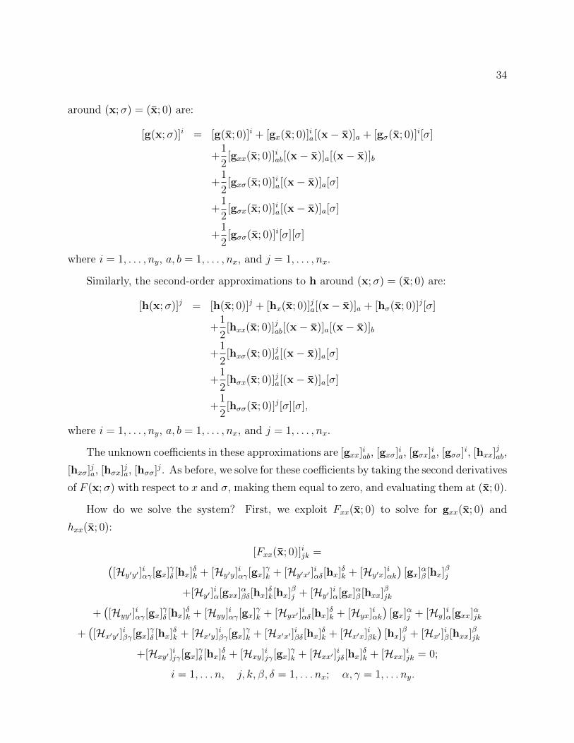
34

around (x;σ) = (x; 0) are:

[g(x;σ)]i = [g(x; 0)]i + [gx(x; 0)]ia[(x− x)]a + [gσ(x; 0)]i[σ]

+1

2[gxx(x; 0)]iab[(x− x)]a[(x− x)]b

+1

2[gxσ(x; 0)]ia[(x− x)]a[σ]

+1

2[gσx(x; 0)]ia[(x− x)]a[σ]

+1

2[gσσ(x; 0)]i[σ][σ]

where i = 1, . . . , ny, a, b = 1, . . . , nx, and j = 1, . . . , nx.

Similarly, the second-order approximations to h around (x;σ) = (x; 0) are:

[h(x;σ)]j = [h(x; 0)]j + [hx(x; 0)]ja[(x− x)]a + [hσ(x; 0)]j[σ]

+1

2[hxx(x; 0)]jab[(x− x)]a[(x− x)]b

+1

2[hxσ(x; 0)]ja[(x− x)]a[σ]

+1

2[hσx(x; 0)]ja[(x− x)]a[σ]

+1

2[hσσ(x; 0)]j[σ][σ],

where i = 1, . . . , ny, a, b = 1, . . . , nx, and j = 1, . . . , nx.

The unknown coefficients in these approximations are [gxx]iab, [gxσ]ia, [gσx]

ia, [gσσ]i, [hxx]

jab,

[hxσ]ja, [hσx]ja, [hσσ]j. As before, we solve for these coefficients by taking the second derivatives

of F (x;σ) with respect to x and σ, making them equal to zero, and evaluating them at (x; 0).

How do we solve the system? First, we exploit Fxx(x; 0) to solve for gxx(x; 0) and

hxx(x; 0):

[Fxx(x; 0)]ijk =([Hy′y′ ]

iαγ[gx]

γδ [hx]

δk + [Hy′y]

iαγ[gx]

γk + [Hy′x′ ]

iαδ[hx]

δk + [Hy′x]

iαk

)[gx]

αβ [hx]

βj

+[Hy′ ]iα[gxx]

αβδ[hx]

δk[hx]

βj + [Hy′ ]

iα[gx]

αβ [hxx]

βjk

+([Hyy′ ]

iαγ[gx]

γδ [hx]

δk + [Hyy]

iαγ[gx]

γk + [Hyx′ ]

iαδ[hx]

δk + [Hyx]

iαk

)[gx]

αj + [Hy]

iα[gxx]

αjk

+([Hx′y′ ]

iβγ[gx]

γδ [hx]

δk + [Hx′y]

iβγ[gx]

γk + [Hx′x′ ]

iβδ[hx]

δk + [Hx′x]

iβk

)[hx]

βj + [Hx′ ]

iβ[hxx]

βjk

+[Hxy′ ]ijγ[gx]

γδ [hx]

δk + [Hxy]

ijγ[gx]

γk + [Hxx′ ]

ijδ[hx]

δk + [Hxx]

ijk = 0;

i = 1, . . . n, j, k, β, δ = 1, . . . nx; α, γ = 1, . . . ny.

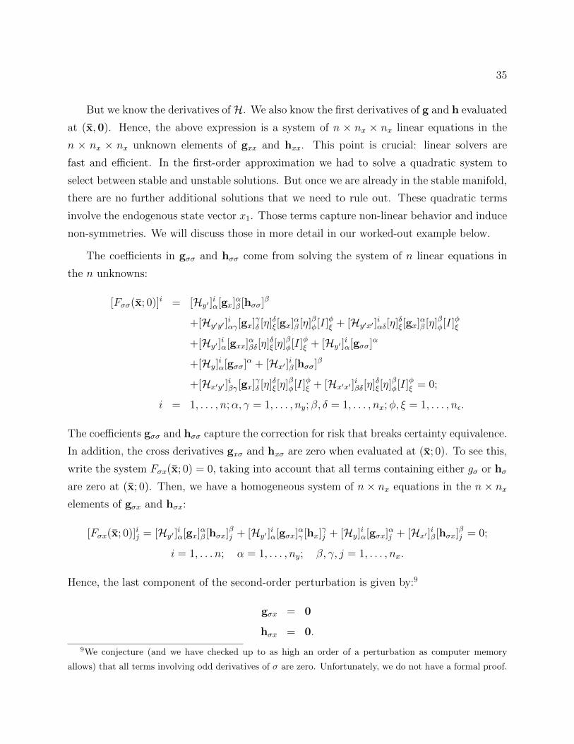
35

But we know the derivatives ofH. We also know the first derivatives of g and h evaluated

at (x,0). Hence, the above expression is a system of n × nx × nx linear equations in the

n × nx × nx unknown elements of gxx and hxx. This point is crucial: linear solvers are

fast and efficient. In the first-order approximation we had to solve a quadratic system to

select between stable and unstable solutions. But once we are already in the stable manifold,

there are no further additional solutions that we need to rule out. These quadratic terms

involve the endogenous state vector x1. Those terms capture non-linear behavior and induce

non-symmetries. We will discuss those in more detail in our worked-out example below.

The coefficients in gσσ and hσσ come from solving the system of n linear equations in

the n unknowns:

[Fσσ(x; 0)]i = [Hy′ ]iα[gx]

αβ [hσσ]β

+[Hy′y′ ]iαγ[gx]

γδ [η]δξ[gx]

αβ [η]βφ[I]φξ + [Hy′x′ ]

iαδ[η]δξ[gx]

αβ [η]βφ[I]φξ

+[Hy′ ]iα[gxx]

αβδ[η]δξ[η]βφ[I]φξ + [Hy′ ]

iα[gσσ]α

+[Hy]iα[gσσ]α + [Hx′ ]

iβ[hσσ]β

+[Hx′y′ ]iβγ[gx]

γδ [η]δξ[η]βφ[I]φξ + [Hx′x′ ]

iβδ[η]δξ[η]βφ[I]φξ = 0;

i = 1, . . . , n;α, γ = 1, . . . , ny; β, δ = 1, . . . , nx;φ, ξ = 1, . . . , nε.

The coefficients gσσ and hσσ capture the correction for risk that breaks certainty equivalence.

In addition, the cross derivatives gxσ and hxσ are zero when evaluated at (x; 0). To see this,

write the system Fσx(x; 0) = 0, taking into account that all terms containing either gσ or hσ

are zero at (x; 0). Then, we have a homogeneous system of n × nx equations in the n × nxelements of gσx and hσx:

[Fσx(x; 0)]ij = [Hy′ ]iα[gx]

αβ [hσx]

βj + [Hy′ ]

iα[gσx]

αγ [hx]

γj + [Hy]

iα[gσx]

αj + [Hx′ ]

iβ[hσx]

βj = 0;

i = 1, . . . n; α = 1, . . . , ny; β, γ, j = 1, . . . , nx.

Hence, the last component of the second-order perturbation is given by:9

gσx = 0

hσx = 0.

9We conjecture (and we have checked up to as high an order of a perturbation as computer memory

allows) that all terms involving odd derivatives of σ are zero. Unfortunately, we do not have a formal proof.

36

4.2.6 Higher-Order Perturbations

We can iterate the previous procedure (taking higher-order derivatives, plugging in the al-

ready found terms, and solving for the remaining ones) as many times as we want to obtain

n-th order approximations. All the associated systems of equations that we would need to

solve are linear, which keeps the computational complexity manageable. The only additional

point to remember is that we will need to make assumptions about the higher moments of

the innovations, as we will have expectational terms involving these higher moments.

If the functions g and h are analytic in a neighborhood of x, then the series we are

building by taking higher-order approximations has an infinite number of terms and is con-

vergent. However, its convergence will occur only in a radius of convergence centered around

x. Disappointingly, for most DSGE models, the radius of convergence (i.e., the r such that

for all state values with a distance with respect to x smaller then r) is unknown (for more

details and an example, see Aldrich and Kung (2011)). More research on this topic is sorely

needed. Also, even when the series is convergent, there are two potential problems. First,

at a j-th order approximation, we may lose the “right” shape of g and h. For example,

Aruoba, Fernandez-Villaverde, and Rubio-Ramırez (2006) document how the decision rules

for consumption and capital of the stochastic neoclassical growth model approximated with

a fifth-order perturbation are no longer globally concave, as implied by economic theory. In-

stead, the approximated functions present oscillating patterns. Second, the convergence to

the exact solution may not be monotone: it is easy to build examples where the errors a bit

away from x are worse for a j+1-th order approximation than for a j-th order approximation.

Later, we will discuss how to gauge the accuracy of a solution and how to decide whether a

higher-order approximation is required. For example, to deal with models with time-varying

volatility, we would need at least a third-order approximation. Levintal (2015) has argued

that to approximate well models with disaster risk, we need a fifth-order approximation. The

drawback of higher-order approximations is that we will run into problems of computational

cost and memory use.

4.3 A Worked-Out Example

The previous derivations were somewhat abstract and the notation, even using tensors, bur-

densome. Consequently, it is useful to show how perturbation works in a concrete example.

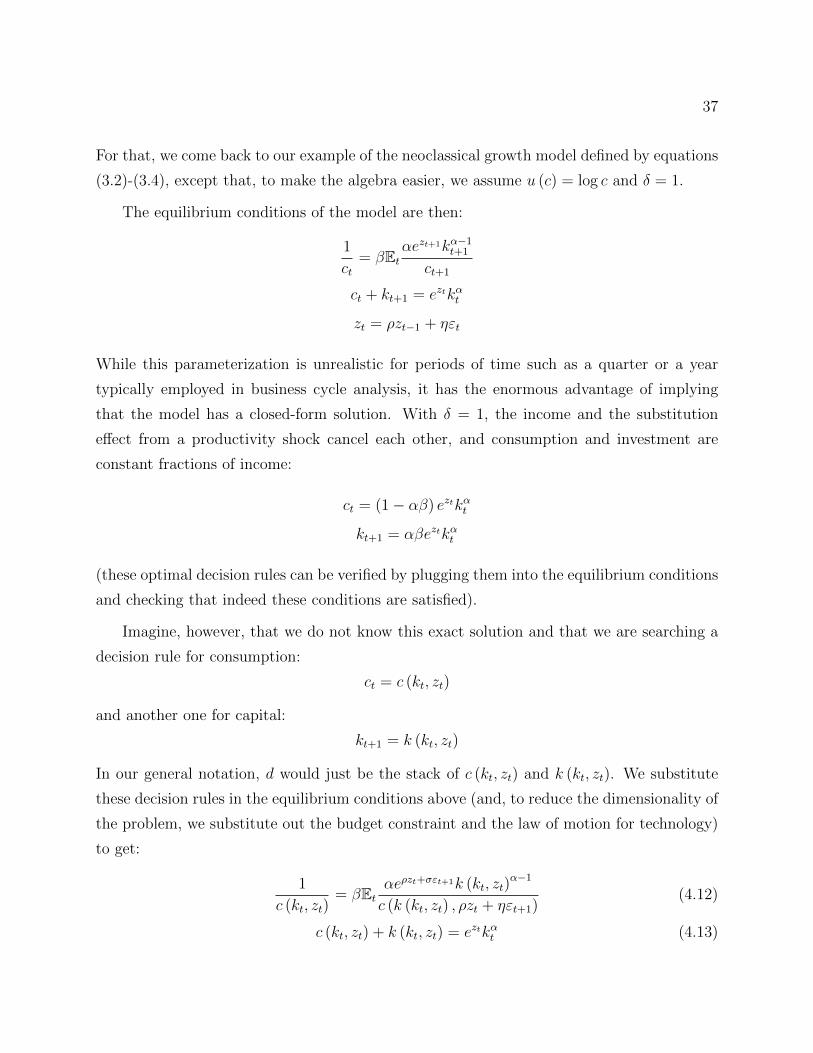
37

For that, we come back to our example of the neoclassical growth model defined by equations

(3.2)-(3.4), except that, to make the algebra easier, we assume u (c) = log c and δ = 1.

The equilibrium conditions of the model are then:

1

ct= βEt

αezt+1kα−1t+1

ct+1

ct + kt+1 = eztkαt

zt = ρzt−1 + ηεt

While this parameterization is unrealistic for periods of time such as a quarter or a year

typically employed in business cycle analysis, it has the enormous advantage of implying

that the model has a closed-form solution. With δ = 1, the income and the substitution

effect from a productivity shock cancel each other, and consumption and investment are

constant fractions of income:

ct = (1− αβ) eztkαt

kt+1 = αβeztkαt

(these optimal decision rules can be verified by plugging them into the equilibrium conditions

and checking that indeed these conditions are satisfied).

Imagine, however, that we do not know this exact solution and that we are searching a

decision rule for consumption:

ct = c (kt, zt)

and another one for capital:

kt+1 = k (kt, zt)

In our general notation, d would just be the stack of c (kt, zt) and k (kt, zt). We substitute

these decision rules in the equilibrium conditions above (and, to reduce the dimensionality of

the problem, we substitute out the budget constraint and the law of motion for technology)

to get:

1

c (kt, zt)= βEt

αeρzt+σεt+1k (kt, zt)α−1

c (k (kt, zt) , ρzt + ηεt+1)(4.12)

c (kt, zt) + k (kt, zt) = eztkαt (4.13)

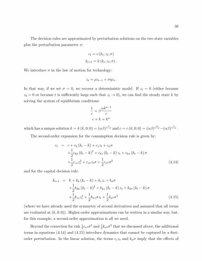
38

The decision rules are approximated by perturbation solutions on the two state variables

plus the perturbation parameter σ:

ct = c (kt, zt;σ)

kt+1 = k (kt, zt;σ) .

We introduce σ in the law of motion for technology:

zt = ρzt−1 + σηεt.

In that way, if we set σ = 0, we recover a deterministic model. If zt = 0 (either because

z0 = 0 or because t is sufficiently large such that zt → 0), we can find the steady state k by

solving the system of equilibrium conditions:

1

c= β

αkα−1

c

c+ k = kα

which has a unique solution k = k (k, 0; 0) = (αβ)1

1−α and c = c (k, 0; 0) = (αβ)α

1−α−(αβ)1

1−α .

The second-order expansion for the consumption decision rule is given by:

ct = c+ ck (kt − k) + czzt + cσσ

+1

2ckk (kt − k)2 + ckz (kt − k) zt + ckσ (kt − k)σ

+1

2czzz

2t + czσztσ +

1

2cσ2σ2 (4.14)

and for the capital decision rule:

kt+1 = k + kk (kt − k) + kzzt + kσσ

+1

2kkk (kt − k)2 + kkz (kt − k) zt + kkσ (kt − k)σ

+1

2kzzz

2t +

1

2kσzσzt +

1

2kσ2σ2 (4.15)

(where we have already used the symmetry of second derivatives and assumed that all terms

are evaluated at (k, 0; 0)). Higher-order approximations can be written in a similar way, but,

for this example, a second-order approximation is all we need.

Beyond the correction for risk 12cσ2σ2 and 1

2kσ2σ2 that we discussed above, the additional

terms in equations (4.14) and (4.15) introduce dynamics that cannot be captured by a first-

order perturbation. In the linear solution, the terms czzt and kσσ imply that the effects of

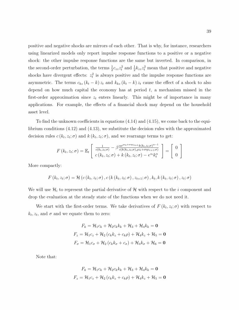
39

positive and negative shocks are mirrors of each other. That is why, for instance, researchers

using linearized models only report impulse response functions to a positive or a negative

shock: the other impulse response functions are the same but inverted. In comparison, in

the second-order perturbation, the terms 12czzz

2t and 1

2kzzz

2t mean that positive and negative

shocks have divergent effects: z2t is always positive and the impulse response functions are

asymmetric. The terms ckz (kt − k) zt and kkz (kt − k) zt cause the effect of a shock to also

depend on how much capital the economy has at period t, a mechanism missed in the

first-order approximation since zt enters linearly. This might be of importance in many

applications. For example, the effects of a financial shock may depend on the household

asset level.

To find the unknown coefficients in equations (4.14) and (4.15), we come back to the equi-

librium conditions (4.12) and (4.13), we substitute the decision rules with the approximated

decision rules c (kt, zt;σ) and k (kt, zt;σ), and we rearrange terms to get:

F (kt, zt;σ) = Et

[1

c(kt,zt;σ)− β αeρzt+σηεt+1k(kt,zt;σ)α−1

c(k(kt,zt;σ),ρzt+σηεt+1;σ)

c (kt, zt;σ) + k (kt, zt;σ)− eztkαt

]=

[0

0

]

More compactly:

F (kt, zt;σ) = H (c (kt, zt;σ) , c (k (kt, zt;σ) , zt+1;σ) , kt, k (kt, zt;σ) , zt;σ)

We will use Hi to represent the partial derivative of H with respect to the i component and

drop the evaluation at the steady state of the functions when we do not need it.

We start with the first-order terms. We take derivatives of F (kt, zt;σ) with respect to

kt, zt, and σ and we equate them to zero:

Fk = H1ck +H2ckkk +H3 +H4kk = 0

Fz = H1cz +H2 (ckkz + ckρ) +H4kz +H5 = 0

Fσ = H1cσ +H2 (ckkσ + cσ) +H4kσ +H6 = 0

Note that:

Fk = H1ck +H2ckkk +H3 +H4kk = 0

Fz = H1cz +H2 (ckkz + ckρ) +H4kz +H5 = 0

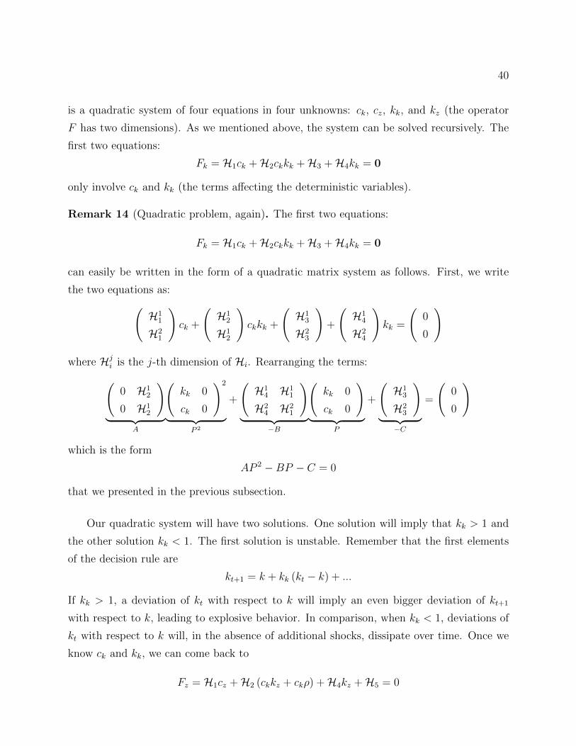
40

is a quadratic system of four equations in four unknowns: ck, cz, kk, and kz (the operator

F has two dimensions). As we mentioned above, the system can be solved recursively. The

first two equations:

Fk = H1ck +H2ckkk +H3 +H4kk = 0

only involve ck and kk (the terms affecting the deterministic variables).

Remark 14 (Quadratic problem, again). The first two equations:

Fk = H1ck +H2ckkk +H3 +H4kk = 0

can easily be written in the form of a quadratic matrix system as follows. First, we write

the two equations as:(H1

1

H21

)ck +

(H1

2

H12

)ckkk +

(H1

3

H23

)+

(H1

4

H24

)kk =

(0

0

)

where Hji is the j-th dimension of Hi. Rearranging the terms:(

0 H12

0 H12

)︸ ︷︷ ︸

A

(kk 0

ck 0

)2

︸ ︷︷ ︸P 2

+

(H1

4 H11

H24 H2

1

)︸ ︷︷ ︸

−B

(kk 0

ck 0

)︸ ︷︷ ︸

P

+

(H1

3

H23

)︸ ︷︷ ︸−C

=

(0

0

)

which is the form

AP 2 −BP − C = 0

that we presented in the previous subsection.

Our quadratic system will have two solutions. One solution will imply that kk > 1 and

the other solution kk < 1. The first solution is unstable. Remember that the first elements

of the decision rule are

kt+1 = k + kk (kt − k) + ...

If kk > 1, a deviation of kt with respect to k will imply an even bigger deviation of kt+1

with respect to k, leading to explosive behavior. In comparison, when kk < 1, deviations of

kt with respect to k will, in the absence of additional shocks, dissipate over time. Once we

know ck and kk, we can come back to

Fz = H1cz +H2 (ckkz + ckρ) +H4kz +H5 = 0

41

and solve for cz and kz. As emphasized in Remark 12, this system is linear.

Finally, as in the general case, the last two equations

Fσ = H1cσ +H2 (ckkσ + cσ) +H4kσ +H6 = 0

form a linear, and homogeneous system in cσ and kσ. Hence, cσ = kσ = 0 and we obtain the

certainty equivalence of first-order approximations.

To find the second-order approximation, we take second derivatives of F (kt, zt;σ) around

k, 0, and 0:

Fkk = 0

Fkz = 0

Fkσ = 0

Fzz = 0

Fzσ = 0

Fσσ = 0

(where we have already eliminated symmetric second derivatives). We substitute the coeffi-

cients that we already know from the first-order approximation and we get a linear system

of 12 equations in 12 unknowns. Again, we get that all cross-terms on kσ and zσ are zero.

Imposing the results concerning the coefficients that are equal to zero, we can rewrite

equations (4.14) and (4.15) up to second-order as:

ct = c+ ck (kt − k) + czzt

+1

2ckk (kt − k)2 + ckz (kt − k) zt +

1

2czzz

2t +

1

2cσ2σ2 (4.16)

and

kt+1 = k + kk (kt − k) + kzzt

+1

2kkk (kt − k)2 + kkz (kt − k) zt +

1

2kzzz

2t +

1

2kσ2σ2. (4.17)

Since even with this simple neoclassical growth model the previous systems of equations

are too involved to be written explicitly, we illustrate the procedure numerically. In Table 1,

we summarize the parameter values for the four parameters of the model. We do not pretend

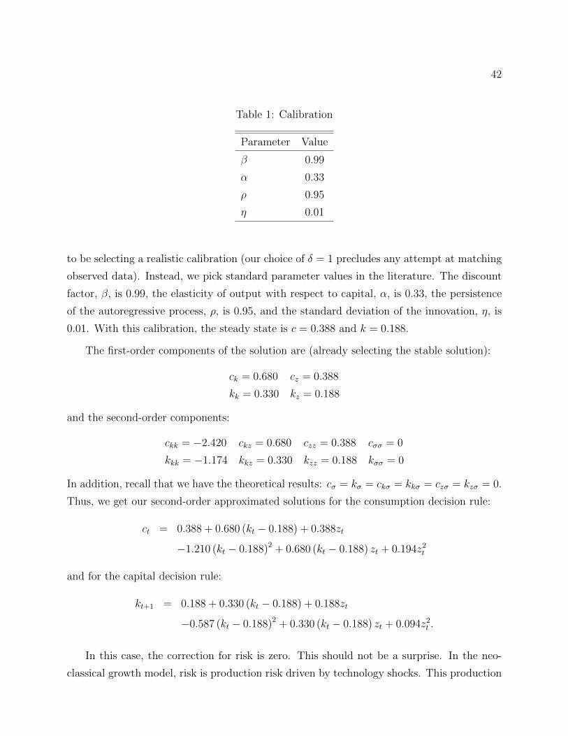
42

Table 1: Calibration

Parameter Value

β 0.99

α 0.33

ρ 0.95

η 0.01

to be selecting a realistic calibration (our choice of δ = 1 precludes any attempt at matching

observed data). Instead, we pick standard parameter values in the literature. The discount

factor, β, is 0.99, the elasticity of output with respect to capital, α, is 0.33, the persistence

of the autoregressive process, ρ, is 0.95, and the standard deviation of the innovation, η, is

0.01. With this calibration, the steady state is c = 0.388 and k = 0.188.

The first-order components of the solution are (already selecting the stable solution):

ck = 0.680 cz = 0.388

kk = 0.330 kz = 0.188

and the second-order components:

ckk = −2.420 ckz = 0.680 czz = 0.388 cσσ = 0

kkk = −1.174 kkz = 0.330 kzz = 0.188 kσσ = 0

In addition, recall that we have the theoretical results: cσ = kσ = ckσ = kkσ = czσ = kzσ = 0.

Thus, we get our second-order approximated solutions for the consumption decision rule:

ct = 0.388 + 0.680 (kt − 0.188) + 0.388zt

−1.210 (kt − 0.188)2 + 0.680 (kt − 0.188) zt + 0.194z2t

and for the capital decision rule:

kt+1 = 0.188 + 0.330 (kt − 0.188) + 0.188zt

−0.587 (kt − 0.188)2 + 0.330 (kt − 0.188) zt + 0.094z2t .

In this case, the correction for risk is zero. This should not be a surprise. In the neo-

classical growth model, risk is production risk driven by technology shocks. This production

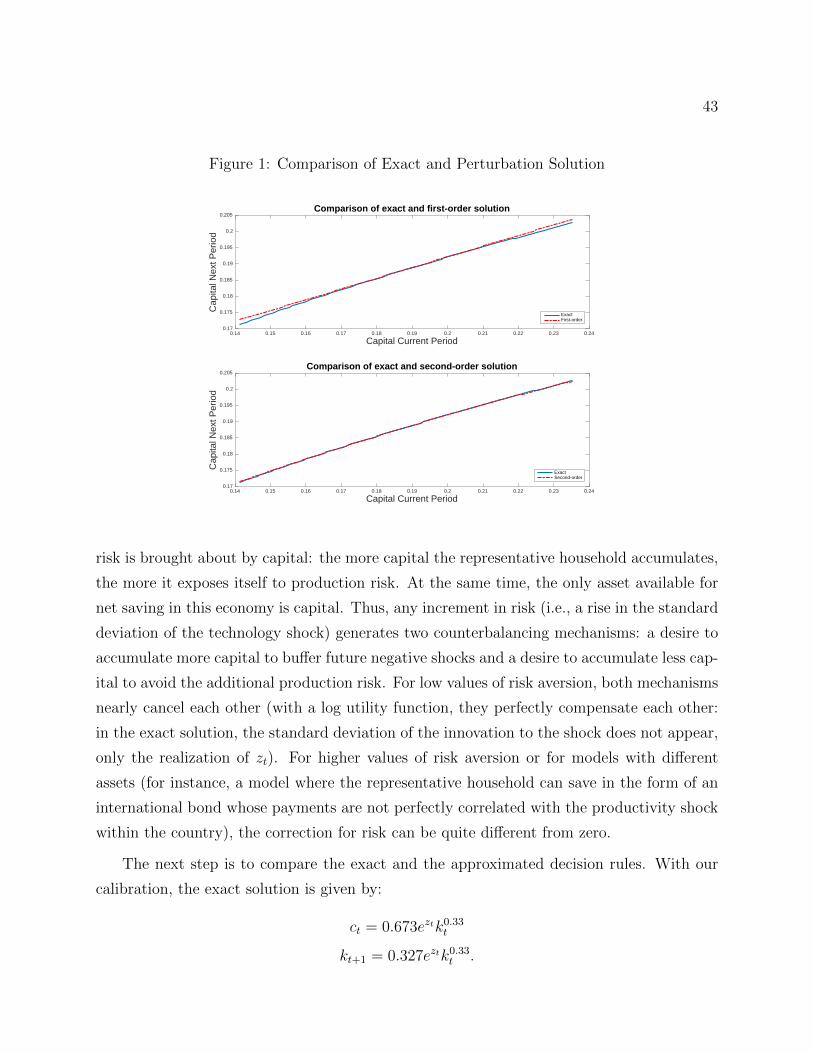
43

Figure 1: Comparison of Exact and Perturbation Solution

0.14 0.15 0.16 0.17 0.18 0.19 0.2 0.21 0.22 0.23 0.24

Capital Current Period

0.17

0.175

0.18

0.185

0.19

0.195

0.2

0.205C

apita

l Nex

t Per

iod

Comparison of exact and first-order solution

ExactFirst-order

0.14 0.15 0.16 0.17 0.18 0.19 0.2 0.21 0.22 0.23 0.24

Capital Current Period

0.17

0.175

0.18

0.185

0.19

0.195

0.2

0.205

Cap

ital N

ext P

erio

d

Comparison of exact and second-order solution

ExactSecond-order

risk is brought about by capital: the more capital the representative household accumulates,

the more it exposes itself to production risk. At the same time, the only asset available for

net saving in this economy is capital. Thus, any increment in risk (i.e., a rise in the standard

deviation of the technology shock) generates two counterbalancing mechanisms: a desire to

accumulate more capital to buffer future negative shocks and a desire to accumulate less cap-

ital to avoid the additional production risk. For low values of risk aversion, both mechanisms

nearly cancel each other (with a log utility function, they perfectly compensate each other:

in the exact solution, the standard deviation of the innovation to the shock does not appear,

only the realization of zt). For higher values of risk aversion or for models with different

assets (for instance, a model where the representative household can save in the form of an

international bond whose payments are not perfectly correlated with the productivity shock

within the country), the correction for risk can be quite different from zero.

The next step is to compare the exact and the approximated decision rules. With our

calibration, the exact solution is given by:

ct = 0.673eztk0.33t

kt+1 = 0.327eztk0.33t .

44

To gauge how close these two solutions are, we plot in Figure 1 the exact decision rule

for capital (continuous line in the top and bottom panels), the first-order approximation

(discontinuous line in the top panel), and the second-order approximation (discontinuous

line in the bottom panel). In both panels, we plot the decision rule for capital when zt = 0

and for values of capital that are ±25 percent of the value of capital in the steady state. The

first-order approximation is nearly identical to the exact solution close to the steady state.

Only farther away, do both solutions diverge. At the start of the grid (with k = 0.1412),

the exact decision rule and the first-order approximation diverge by nearly 1 percent. The

second-order approximation, in comparison, is more accurate along the whole range of values

of capital. Even at k = 0.1412, the difference between both solutions is only 0.13 percent.

This result shows the often good global properties of perturbation solutions.

We will revisit below how to assess the accuracy of a solution. Suffice it to say at this

moment that whether 0.13 percent is too large or accurate enough is application dependent.

For instance, for the computation of business cycle moments, we often need less accuracy

than for welfare evaluations. The reason is that while errors in the approximation of a

moment of the model, such as the mean or variance of consumption, tend to cancel each

other, welfare is a non-linear function of the allocation and small errors in computing an

allocation can translate into large errors in computing welfare.

4.4 Pruning

Although the higher-order perturbations that we described are intuitive and straightforward

to compute, they often generate explosive sample paths even when the corresponding linear

approximation is stable. These explosive sample paths arise because the higher-order terms

induce additional fixed points for the system, around which the approximated solution is

unstable (see Kim, Kim, Schaumburg, and Sims (2008), and Den Haan and De Wind (2012)).

A simple example clarifies this point. Imagine that we have an approximated decision rule

for capital (where, for simplicity, we have eliminated the persistence on the productivity

process zt) that has the form:

kt+1 = a0 + a1kt + a2k2t + . . .+ b1εt + . . .

If we substitute recursively, we find:

kt+1 = a1kt + a2

(a1kt−1 + a2k

2t−1

)2+ . . .+ b1εt + . . . ,

45

an expression that involves terms in k3t−2 and k4

t−2. If the support of εt is not bounded, sooner

or later, we will have, in a simulation, an innovation large enough such that kt+1 is far away

from its steady-state value. As the simulation progresses over time, that value of kt+1 will be

raised to cubic and higher-order powers, and trigger an explosive path. The presence of this

explosive behavior complicates any model evaluation because no unconditional moments

would exist based on this approximation. It also means that any unconditional moment-

matching estimation methods, such as the generalized method of moments (GMM) or the

simulated method of moments (SMM), are inapplicable in this context as they rely on finite

moments from stationary and ergodic probability distributions.

For second-order approximations, Kim, Kim, Schaumburg, and Sims (2008) propose

pruning the approximation. Loosely speaking, pruning means to eliminate, in the recursions,

all terms that are of a higher order than the order of the solution (i.e., if we are dealing with a

second-order perturbation, all terms involving states or innovations raised to powers higher

than 2). Kim, Kim, Schaumburg, and Sims (2008) prove that the pruned approximation

does not explode.

Andreasen, Fernandez-Villaverde, and Rubio-Ramırez (2013) extend Kim, Kim, Schaum-

burg, and Sims (2008)’s approach by showing how to apply pruning to an approximation

of any arbitrary order by exploiting what the authors refer to as the pruned state-space

system. Under general technical conditions, Andreasen, Fernandez-Villaverde, and Rubio-

Ramırez (2013) show that first and second unconditional moments for a pruned state-space

system exist. Then, they provide closed-form expressions for first and second unconditional

moments and impulse response functions. This is important because these expressions let

researchers avoid the use of numerical simulations to compute these moments. These nu-

merical simulations have often been shown to be unreliable, in particular, when solving

for the generalized impulse response functions of DSGE models (for the definition of gen-

eralized impulse response functions, see Koop, Pesaran, and Potter (1996)). Andreasen,

Fernandez-Villaverde, and Rubio-Ramırez (2013) also derive conditions for the existence of

higher unconditional moments, such as skewness and kurtosis.

46

4.5 Change of Variables

In Remark 4, we discussed the possibility of performing the perturbation of a DSGE model in

logs of the variables of interest, instead of doing it in levels. In a creative contribution, Judd

(2003) argues that loglinearization is a particular case of the more general idea of a change of

variables and shows how this technique could be efficiently implemented. In this subsection,

we explain Judd’s contribution by following Fernandez-Villaverde and Rubio-Ramırez (2006).

The point of departure is to note that if we have a Taylor expansion of a variable x

around a point a:

d (x) ' d (a) +∂d (a)

∂a(x− a) +H.O.T.,

(where H.O.T. stands for higher-order terms), we can rewrite the expansion in terms of a

transformed variable Y (x):

g (y) = h (d (X (y))) = g (b) +∂g (b)

∂b(Y (x)− b) +H.O.T.

where b = Y (a) and X (y) is the inverse of Y (x). Since with a perturbation we find a Taylor

series approximation of the unknown function d that solves the operator H (·) as a function

of the states x, the change of variables means we can find an alternative Taylor series in

terms of Y (x).

Why do we want to perform this change of variables? The famous British meteorologist

Eric Eady (1915 – 1966) remarked once that: “It is not the process of linearization that

limits insight. It is the nature of the state that we choose to linearize about.” By picking

the right change of variables, we can reshape a highly non-linear problem into a much more

linear one and, therefore, significantly increase the accuracy of the perturbation.10

4.5.1 A Simple Example

Imagine that our aim is to approximate the decision rule for capital in our workhorse stochas-

tic neoclassical growth model with a first-order perturbation (the same ideas would apply

10An idea related to the change of variables is the use of gauges, where the perturbation is undertaken

not in terms of powers of the perturbation parameter, σ, but of a series of gauge functions δn (σ)∞n=1 such

that:

limn→∞

δn+1 (σ)

δn (σ)= 0.

See Judd (1998) for details.

47

if we are trying to approximate other decision rules, expectations, value functions, etc.).

Remember that we derived that such an approximation had the form:

kt+1 = k + a1 (kt − k) + b1zt

where a and b are the coefficients that we find by taking derivatives of F (kt, zt;σ) and k is

the steady-state value of capital. In this section, it is more convenient to rewrite the decision

rule as:

(kt+1 − k) = a1 (kt − k) + b1zt.

Analogously a loglinear approximation of the policy function will take the form:

log kt+1 − log k = a2 (log kt − log k) + b2z

or in equivalent notation:

kt+1 = a2kt + b2zt

where x = log x − log x0 is the percentage deviation of the variable x with respect to its

steady state.

How do we go from one approximation to the second one? First, we write the linear

system in levels as:

kt+1 = d(kt, zt;σ) = d (k, 0; 0) + d1 (k, 0; 0) (kt − k) + d2 (k, 0; 0) zt

where d (k, 0; 0) = k, d1 (k, 0; 0) = a1, d2 (k, 0; 0) = b1. Second, we propose the changes of

variables h = log d, where Y (x) = log x and Y (x) = log x. Third, we apply Judd (2003)’s

formulae for this example:

log kt+1 − log k = d1 (k, 0, 0) (log kt − log k) +1

kd2 (k, 0, 0) z

Finally, by equating coefficients, we obtain a simple closed-form relation between the param-

eters of both representations: a2 = a1 and b2 = 1kb1.

Three points are important. First, moving from a1 and b1 to a2 and b2 is an operation

that only involves k, a value that we already know from the computation of the first-order

perturbation in levels. Therefore, once the researcher has access to the linear solution,

obtaining the loglinear one is immediate.11 Second, we have not used any assumption on the

11A heuristic argument that delivers the same result takes:

(kt+1 − k) = a1 (kt − k) + b1zt

48

utility or production functions except that they satisfy the general technical conditions of

the stochastic neoclassical growth model. Third, the change of variables can be applied to a

perturbation of an arbitrary order. We only presented the case for a first-order approximation

to keep the exposition succinct.

4.5.2 A More General Case

We can now present a more general case of change of variables. The first-order solution of a

model is:

d (x) ' d (a) +∂d (a)

∂a(x− a) .

If we expand g(y) = h (d (X (y))) around b = Y (a), where X (y) is the inverse of Y (x), we

can write:

g (y) = h (d (X (y))) = g (b) + gα (b) (Y α (x)− bα)

where gα = hAdAi X

iα comes from the application of the chain rule.

Following Judd (2003), we use this approach to encompass any power function approxi-

mation of the form:

kt+1 (k, z; γ, ζ, ϕ)γ − kγ = a3

(kζt − kζ

)+ b3z

ϕ

where we impose ϕ ≥ 1 to ensure that we have real values for the power zϕ. Power functions

are attractive because, with only three free parameters (γ, ζ, ϕ), we can capture many non-

linear structures and nest the log transformation as the limit case when the coefficients γ

and ζ tend to zero and ϕ = 1. The changes of variables for this family of functions are given

by h = dγ, Y = xζ , and X = y1ζ . Following the same reasoning as before, we derive:

kt+1 (k, z; γ, ζ, ϕ)γ − kγ =γ

ζkγ−ζa1

(kζt − kζ

)+γ

ϕkγ−1b1z

ϕ.

The relation between the new and the old coefficients is again easy to compute: a3 = γζkγ−ζa1

and b3 = γϕkγ−1b1.

and divides on both sides by k:kt+1 − k

k= a1

kt − kk

+1

kb1z.

Noticing that xt−xx ' log xt − log x, we get back the same relation as the one above. Our argument in the

main text is more general and does not depend on an additional approximation.

49

A slightly more restrictive case is to impose that γ = ζ and z = 1. Then, we get a power

function with only one free parameter γ:

kt+1 (k, z; γ)γ − kγ = a4

(kζt − kζ

)+ b4z

or, by defining kt = kγt − kγ, we get:

kt+1 = a4kt + b4z

with a4 = a1 and b4 = kγ−1b1. This representation has the enormous advantage of being a

linear system, which makes it suitable for analytic study and, as we will see in Section 10,

for estimation with a Kalman filter.

4.5.3 The Optimal Change of Variables

The previous subsection showed how to go from a first-order approximation to the solution of

a DSGE model to a more general representation indexed by some parameters. The remaining

question is how to select the optimal value of these parameters.12

Fernandez-Villaverde and Rubio-Ramırez (2006) argue that a reasonable criterion (and

part of the motivation for the change of variables) is to select these parameters to improve

the accuracy of the solution of the model. More concretely, the authors propose to minimize

the Euler error function with respect to some metric. Since we have not introduced the

measures of accuracy of the solution to a DSGE model, we will skip the details of how to

do so. Suffice it to say that Fernandez-Villaverde and Rubio-Ramırez (2006) find that the

optimal change of variables improves the average accuracy of the solution by a factor of

around three. This improvement makes a first-order approximation competitive in terms

of accuracy with much more involved methods. Fernandez-Villaverde and Rubio-Ramırez

(2006) also report that the optimal parameter values depend on the standard deviation of

the exogenous shocks to the economy. This is a significant result: the change of variables

corrects by the level of uncertainty existing in the economy and breaks certainty equivalence.

12We do not even need to find the optimal value of these parameters. It may be the case that a direct but

not optimal choice of parameter values already delivers substantial improvements in accuracy at a very low

computational cost. When one is maximizing, for example, a likelihood function, being at the true maximum

matters. When one is finding parameters that improve accuracy, optimality is desirable but not essential,

and it can be traded off against computational cost.

50

Remark 15 (Loglinearization v. lognormal-loglinear approximation). A different solution

technique, called lognormal-loglinear approximation, is popular in finance. Its relation with

standard loglinearization (as a particular case of first-order perturbation with a change of

variables in logs) often causes confusion among researchers and students. Thus, once we

have understood the change of variables technique, it is worthwhile to dedicate this remark

to clarifying the similarities and differences between the first-order perturbation in logs

and the lognormal-loglinear approximation. The best way to illustrate this point is with a

concrete example. Imagine that we have a household with utility function

maxE0

∞∑t=0

βt logCt

and budget constraint:

Wt+1 = Rt+1 (Wt − Ct)where Wt is total wealth and W0 is given. Then, the optimality conditions are:

1 = βEtCtCt+1

Rt+1

Wt+1 = Rt+1 (Wt − Ct)

with steady state R = 1β

and W = R (W − C) .

Under a standard first-order perturbation in logs (loglinearization) around the previous

steady state, and after some algebra:

Et∆ct+1 = Etrt+1

wt+1 = rt+1 +1

ρwt +

(1− 1

ρ

)ct

where, for a variable Xt,

xt = xt − x = logXt − logX

and ρ = W−CW

. Subtracting wt from the second equation:

∆wt+1 = rt+1 +

(1− 1

ρ

)(ct − wt)

If we want to express these two equations in logs, instead of log-deviations (and using the

fact that r = − log β):

Et∆ct+1 = log β + Etrt+1 (4.18)

∆wt+1 = rt+1 + k +

(1− 1

ρ

)(ct − wt) (4.19)

51

where

k = −r −(

1− 1

ρ

)(c− w) .

In comparison, a lognormal-loglinearization still uses the approximation of the budget

constraint (4.19), but it assumes that CtCt+1

Rt+1 is distributed as a lognormal random variable.

Since, for an arbitrary variable:

logEtXt = Et logXt +1

2V art logXt,

we can go back to the Euler equation

1 = βEtCtCt+1

Rt+1

and rewrite it as:

0 = log β + logEtCtCt+1

Rt+1

= log β + Et logCtCt+1

Rt+1 +1

2V art log

CtCt+1

Rt+1

or, rearranging terms:

Et∆ct+1 = log β + Etrt+1 +1

2[V art∆ct+1 + V artrt+1 − 2covt (∆ct+1, rt+1)] (4.20)

More in general, in a lognormal-loglinearization, we approximate the non-expectational equa-

tions with a standard loglinearization and we develop the expectational ones (or at least the

ones with returns on them) using a lognormal assumption. In particular, we do not approx-

imate the Euler equation. Once we have assumed that CtCt+1

Rt+1 is lognormal, all the results

are exact.

If we compare the two equations for the first difference of consumption, (4.18) and (4.20),

we see that the lognormal-loglinear approximation introduces an additional term

1

2[V art∆ct+1 + V artrt+1 − 2covt (∆ct+1, rt+1)]

that breaks certainty equivalence. This novel feature has important advantages. For exam-

ple, for a pricing kernel Mt and an asset i, we have the pricing equation:

1 = EtMt+1Ri,t+1.

52

Then:

0 = Et logMt+1Ri,t+1 +1

2V art logMt+1Ri,t+1

or:

Etri,t+1 = −Etmt+1 −1

2V artmt+1 −

1

2V artri,t+1 − covt (mt+1, ri,t+1)

If we look at the same expression for the risk-free bond:

1 = EtMt+1Rf,t+1

we get:

rf,t+1 = −Etmt+1 −1

2V artmt+1

and we can find that the excess return is:

Etri,t+1 − rf,t+1 = −1

2V artri,t+1 − covt (mt+1, ri,t+1) ,

an expression that it is easy to interpret.

On the other hand, this expression also embodies several problems. First, it is often

unclear to what extent, in a general equilibrium economy, CtCt+1

Rt+1 is close to lognormality.

Second, in lognormal-loglinear approximation, we are mixing two approaches, a lognormal

assumption with a loglinearization. This is not necessarily coherent from the perspective of

perturbation theory and we may lack theoretical foundations for the approach (including an

absence of convergence theorems). Third, in the loglinearization, we can compute all the

coefficients by solving a quadratic matrix system. In the lognormal-loglinear approximation,

we need to compute second moments and, in many applications, how to do so may not be

straightforward. Finally, it is not obvious how to get higher-order approximations with the

lognormal-loglinear approximation, while perturbation theory can easily handle higher-order

solutions.

4.6 Perturbing the Value Function

In some applications, it is necessary to perturb the value function of a DSGE model, for

example, when we are dealing with recursive preferences or when we want to evaluate welfare.

Furthermore, a perturbed value function can be an outstanding initial guess for value function

iteration, making it possible to deal with high-dimensional problems that could be otherwise

53

too slow to converge. Given the importance of perturbing the value function, this section

illustrates in some detail how to do so.

Since all that we learned in the general case subsection will still apply by just changing

the operator H from the equilibrium conditions to the Bellman operator, we can go directly

to a concrete application. Consider a value function problem (following the same notation

as above).

V (kt, zt) = maxct

[(1− β) log ct + βEtV (kt+1, zt+1)]

s.t. ct + kt+1 = eztkαt + (1− δ) ktzt = ρzt−1 + ηεt, εt ∼ N (0, 1)

where we have “normalized” log ct by (1− β) to make the value function and the utility

function have the same order of magnitude (thanks to normalization, Vss = log c, where Vss

is the steady-state value function and c is the steady-state consumption).

We can rewrite the problem in terms of a perturbation parameter σ:

V (kt, zt;σ) = maxct

[log ct + βEtV (eztkαt + (1− δ) kt − ct, ρzt + σηεt+1;σ)] .

Note that we have made explicit the dependencies in the next period states from the current

period state. The perturbation solution of this problem is a value function V (kt, zt;σ)

and a policy function for consumption c (kt, zt;σ). For example, the second-order Taylor

approximation of the value function around the deterministic steady state (k, 0; 0) is:

V (kt, zt;σ) = Vss + V1,ss (kt − k) + V2,sszt + V3,ssσ

+1

2V11,ss (kt − k)2 + V12,ss (kt − k) zt + V13,ss (kt − k)σ

+1

2V22,ssz

2t + V23,ssztσ +

1

2V33,ssσ

2

where:

Vss = V (k, 0; 0)

Vi,ss = Vi (k, 0; 0) for i = 1, 2, 3Vij,ss = Vij (k, 0; 0) for i, j = 1, 2, 3

By certainty equivalence:

V3,ss = V13,ss = V23,ss = 0

54

and then:

V (kt, zt; 1) = Vss + V1,ss (kt − k) + V2,sszt

+1

2V11,ss (kt − k)2 +

1

2V22,ssz

2tt + V12,ss (kt − k) z +

1

2V33,ssσ

2

Note that V33,ss 6= 0, a difference from the LQ approximation to the utility function that we

discussed in Remark 13.

Similarly, the policy function for consumption can be expanded as:

ct = c (kt, zt;σ) = css + c1,ss (kt − k) + c2,sszt + c3,ssσ

where ci,ss = c1 (k, 0; 0) for i = 1, 2, 3. Since the first derivatives of the consumption

function only depend on the first and second derivatives of the value function, we must have

that c3,ss = 0 (remember that precautionary consumption depends on the third derivative

of the value function; Kimball (1990)).

To find the linear components of our approximation to the value function, we take deriva-

tives of the value function with respect to controls (ct), states (kt, zt), and the perturbation

parameter σ and solve the associated system of equations when σ = 0. We can find the

quadratic components of the value function by taking second derivatives, plugging in the

known components from the previous step, and solving the system when σ = 0.

We are ready now to show some of the advantages of perturbing the value function. First,

we have an evaluation of the welfare cost of business cycle fluctuations readily available. At

the deterministic steady state kt = k and zt = 0, we have:

V (k, 0;σ) = Vss +1

2V33,ssσ

2.

Hence 12V33,ssσ

2 is a measure of the welfare cost of the business cycle: it is the difference, up

to second-order, between the value function evaluated at the steady-state value of the state

variables (k, 0) and the steady-state value function (where not only are we at the steady

state, but where we know that in future periods we will be at that point as well). Note that

this last quantity is not necessarily negative. Indeed, it may well be positive in many models,

such as in a stochastic neoclassical growth model with leisure choice. For an explanation

55

and quantitative evidence, see Cho, Cooley, and Kim (2015).13

It is easier to interpret V33,ss if we can transform it into consumption units. To do so,

we compute the decrease in consumption τ that will make the household indifferent between

consuming (1− τ) c units per period with certainty or ct units with uncertainty. That is, τ

satisfies:

log (1− τ) c = log c+1

2V33,ssσ

2

where we have used Vss = log c. Then,

τ = 1− e 12V33,ssσ2

.

We close this section with a numerical application. To do so, we pick the same calibration

as in Table 1. We get:

V (kt, zt; 1) = −0.54000 + 0.026 (kt − 0.188) + 0.250zt − 0.069 (kt − 0.188)2 (4.21)

(where, for this calibration, Vkz = Vz2 = Vσ2 = 0) and:

c (kt, zt;χ) = 0.388 + 0.680 (kt − 0.188) + 0.388zt,

which is the same approximation to the consumption decision rule we found when we tackled

the equilibrium conditions of the model. For this calibration, the welfare cost of the business

cycle is zero.14

We can also use equation (4.21) as an initial guess for value function iteration. Thanks

to it, instead of having to iterate hundreds of times, as if we were starting from a blind initial

guess, value function iteration can converge after only a few dozen interactions.

13In his classical calculation about the welfare cost of the business cycle, Lucas (1987) assumed an endow-

ment economy, where the representative household faces the same consumption process as the one observed

for the U.S. economy. Thus, for any utility function with risk aversion, the welfare cost of the business cycle

must be positive (although Lucas’ point, of course, was that it was rather small). When consumption and

labor supply are endogenous, agents can take advantage of uncertainty to increase their welfare. A direct

utility function that is concave in allocations can generate a convex indirect utility function on prices and

those prices change in general equilibrium as a consequence of the agents’ responses to uncertainty.14Recall that the exact consumption decision rule is ct = 0.673eztk0.33t . Since the utility function is log,

the period utility from this decision rule is log ct = zt + log 0.673 + 0.33 log kt. The unconditional mean of

zt is 0 and the capital decision rule is certainty equivalent in logs. Thus, there is no (unconditional) welfare

cost of changing the variance of zt.

56

Finally, a mixed strategy is to stack both the equilibrium conditions of the model and

the value function evaluated at the optimal decision rules:

V (kt, zt) = (1− β) log ct + βEtV (kt+1, zt+1) .

in the operator H. This strategy delivers an approximation to the value function and the

decision rules with a trivial cost.15

5 Projection

Projection methods (also known as weighted residual methods) handle DSGE models by

building a function indexed by some coefficients that approximately solves the operator H.

The coefficients are selected to minimize a residual function that evaluates how far away the

solution is from generating a zero in H. More concretely, projection methods solve:

H (d) = 0

by specifying a linear combination:

dj (x|θ) =

j∑i=0

θiΨi (x) (5.1)

of basis function Ψi (x) given coefficients θ = θ0, ..., θj. Then, we define a residual function:

R (x|θ) = H(dj (x|θ)

)and we select the values of the coefficients θ that minimize the residual given some metric.

This last step is known as “projecting” H against that basis to find the components of θ

(and hence the name of the method).

Inspection of equation (5.1) reveals that to build the function dj (x|θ), we need to pick

a basis Ψi (x)∞i=0 and decide which inner product we will use to “project” H against that

15We could also stack derivatives of the value function, such as:

(1− β) c−1t − βEtV1,t+1 = 0

and find the perturbation approximation to the derivative of the value function (which can be of interest in

itself or employed in finding higher-order approximations of the value function).

57

basis to compute θ. Different choices of bases and of the projection algorithm will imply

different projection methods. These alternative projections are often called in the literature

by their own particular names, which can be sometimes bewildering.

Projection theory, which has been applied in ad hoc ways by economists over the years,

was popularized as a rigorous approach in economics by Judd (1992) and Gaspar and Judd

(1997) and, as in the case of perturbation, it has been authoritatively presented by Judd

(1998).16

Remark 16 (Linear v. non-linear combinations). Instead of linear combinations of basis

functions, we could deal with more general non-linear combinations:

dj (x|θ) = f(Ψi (x)ji=0 |θ

)for a known function f . However, the theory for non-linear combinations is less well devel-

oped, and we can already capture a full range of non-linearities in dj with the appropriate

choice of basis functions Ψi. In any case, it is more pedagogical to start with the linear

combination case. Most of the ideas in the next pages carry over the case of non-linear

combinations. The fact that we are working with linear combinations of basis functions also

means that, in general, we will have the same number of coefficients θ as the number of basis

functions Ψi times the dimensionality of dj.

5.1 A Basic Projection Algorithm

Conceptually, projection is easier to present than perturbation (although its computational

implementation is harder). We can start directly by outlining a projection algorithm:

Algorithm 1 (Projection Algorithm).

1. Define j + 1 known linearly independent functions ψi : Ω → R where j < ∞. We

call the ψ0, ψ1, ..., ψj the basis functions. These basis functions depend on the vector

of state variables x.16Projection theory is more modern than perturbation. Nevertheless, projection methods have been used

for many decades in the natural sciences and engineering. Spectral methods go back, at least, to Lanczos

(1938). Alexander Hrennikoff and Richard Courant developed the finite elements method in the 1940s,

although the method was christened by Clough (1960), who made pioneering contributions while working at

Boeing. See Clough and Wilson (1999) for a history of the early research on finite elements.

58

2. Define a vector of coefficients θl =[θl0, θ

l1, ..., θ

lj

]for l = 1, ...,m (where recall that m

is the dimension that the function d of interest maps into). Stack all coefficients on a

(j + 1)×m matrix θ =[θ1; θ2; ...; θl

].

3. Define a combination of the basis functions and the θ’s:

dl,j(·| θl)

=

j∑i=0

θliψi (·)

for n = 1, ...,m. Then:

dj ( ·| θ) =[d1,j ( ·| θn) ; d2,j ( ·| θn) ; ...; dm,j ( ·| θn)

].

4. Plug dj ( ·| θ) into the operator H (·) to find the residual equation:

R ( ·| θ) = H(dj ( ·| θ)

).

5. Find the value of θ that makes the residual equation as close to 0 as possible given

some objective function ρ : J2 × J2 → R:

θ = arg minθ∈R(j+1)×m

ρ (R ( ·| θ) ,0) .

To ease notation, we have made two simplifications on the previous algorithm. First,

we assumed that, along each dimension of d, we used the same basis functions ψi and the

same number j + 1 of them. Nothing forces us to do so. At the mere cost of cumbersome

notation, we could have different basis functions for each dimension and a different number

of them (i.e., different j’s). While the former is not too common in practice, the latter is

standard, since some variables’ influence on the function d can be harder to approximate

than others’.17

We specify a metric function ρ to gauge how close the residual function is to zero over

the domain of the state variables. For example, in Figure 2, we plot two different residual

17For the non-linear combination case, f(Ψi (x)ji=0 |θ

), we would just write the residual function:

R ( ·| θ) = H(f(Ψi (x)ji=0 |θ

))and find the θ’s that minimize a given metric. Besides the possible computational complexities of dealing

with arbitrary functions f(Ψi (x)ji=0 |θ

), the conceptual steps are the same.

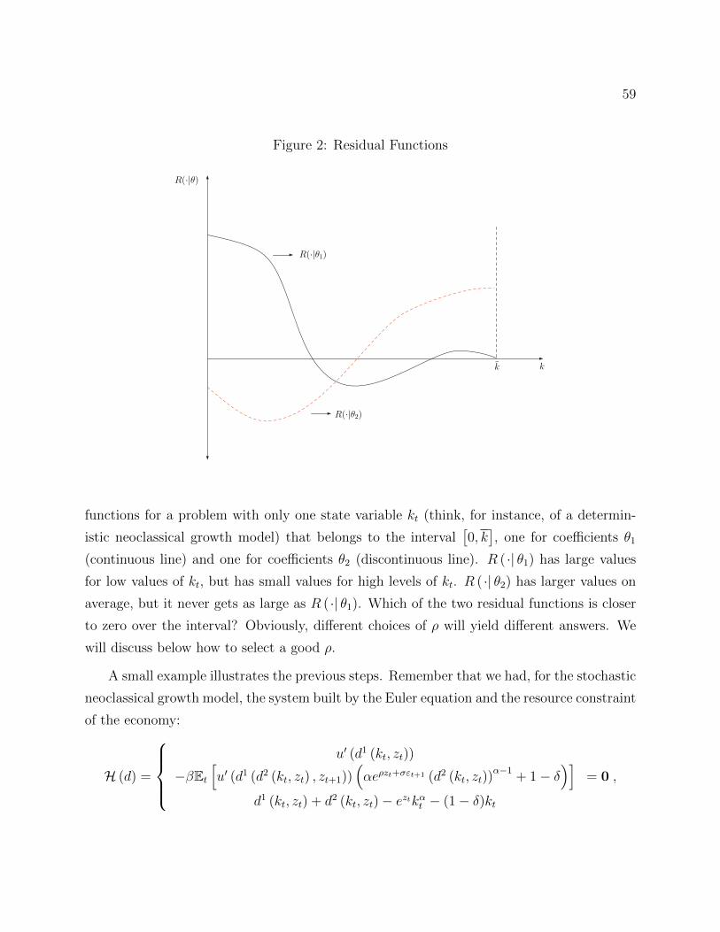
59

Figure 2: Residual FunctionsFigure 1: Insert Title Here

R(·|θ1)

R(·|θ)

k

R(·|θ2)

k

1

functions for a problem with only one state variable kt (think, for instance, of a determin-

istic neoclassical growth model) that belongs to the interval[0, k], one for coefficients θ1

(continuous line) and one for coefficients θ2 (discontinuous line). R ( ·| θ1) has large values

for low values of kt, but has small values for high levels of kt. R ( ·| θ2) has larger values on

average, but it never gets as large as R ( ·| θ1). Which of the two residual functions is closer

to zero over the interval? Obviously, different choices of ρ will yield different answers. We

will discuss below how to select a good ρ.

A small example illustrates the previous steps. Remember that we had, for the stochastic

neoclassical growth model, the system built by the Euler equation and the resource constraint

of the economy:

H (d) =

u′ (d1 (kt, zt))

−βEt[u′ (d1 (d2 (kt, zt) , zt+1))

(αeρzt+σεt+1 (d2 (kt, zt))

α−1+ 1− δ

)]d1 (kt, zt) + d2 (kt, zt)− eztkαt − (1− δ)kt

= 0 ,

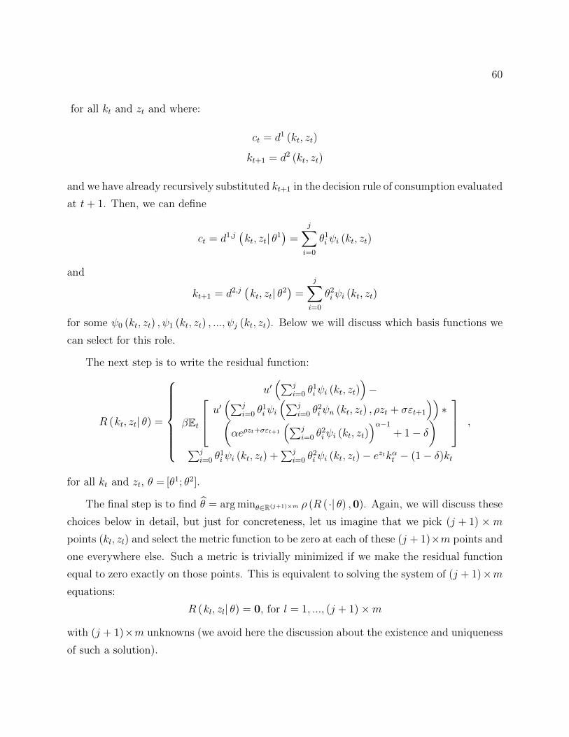
60

for all kt and zt and where:

ct = d1 (kt, zt)

kt+1 = d2 (kt, zt)

and we have already recursively substituted kt+1 in the decision rule of consumption evaluated

at t+ 1. Then, we can define

ct = d1,j(kt, zt| θ1

)=

j∑i=0

θ1iψi (kt, zt)

and

kt+1 = d2,j(kt, zt| θ2

)=

j∑i=0

θ2iψi (kt, zt)

for some ψ0 (kt, zt) , ψ1 (kt, zt) , ..., ψj (kt, zt). Below we will discuss which basis functions we

can select for this role.

The next step is to write the residual function:

R (kt, zt| θ) =

u′(∑j

i=0 θ1iψi (kt, zt)

)−

βEt

u′(∑j

i=0 θ1iψi

(∑ji=0 θ

2iψn (kt, zt) , ρzt + σεt+1

))∗(

αeρzt+σεt+1

(∑ji=0 θ

2iψi (kt, zt)

)α−1

+ 1− δ)

∑ji=0 θ

1iψi (kt, zt) +

∑ji=0 θ

2iψi (kt, zt)− eztkαt − (1− δ)kt

,

for all kt and zt, θ = [θ1; θ2].

The final step is to find θ = arg minθ∈R(j+1)×m ρ (R ( ·| θ) ,0). Again, we will discuss these

choices below in detail, but just for concreteness, let us imagine that we pick (j + 1) × mpoints (kl, zl) and select the metric function to be zero at each of these (j + 1)×m points and

one everywhere else. Such a metric is trivially minimized if we make the residual function

equal to zero exactly on those points. This is equivalent to solving the system of (j + 1)×mequations:

R (kl, zl| θ) = 0, for l = 1, ..., (j + 1)×m

with (j + 1)×m unknowns (we avoid here the discussion about the existence and uniqueness

of such a solution).

61

Remark 17 (Relation to econometrics). Many readers will be familiar with the use of the

word “projection” in econometrics. This is not a coincidence. A common way to present

linear regression is to think about the problem of searching for the unknown conditional

expectation function:

E (Y |X)

for some variables Y and X. Given that this conditional expectation is unknown, we can

approximate it with the first two monomials on X, 1 (a constant) and X (a linear function),

and associated coefficients θ0 and θ1:

E (Y |X) ' θ0 + θ1X.

These two monomials are the first two elements of a basis composed by the monomials (and

also of the Chebyshev polynomials, a basis of choice later in this section). The residual

function is then:

R (Y,X| θ0, θ1) = Y − θ0 − θ1X.

The most common metric in statistical work is to minimize the square of this residual:

R (Y,X| θ0, θ1)2

by plugging in the observed series Y,Xt=1:T . The difference, thus, between ordinary least

squares and the projection algorithm is that while in the former we use observed data, in the

latter we use the operator H (d) imposed by economic theory. This link is even clearer when

we study the econometrics of semi-nonparametric methods, such as sieves (Chen (2007)),

which look for flexible basis functions indexed by a low number of coefficients and that,

nevertheless, impose fewer restrictions than a linear regression.

Remark 18 (Comparison with other methods). From our short description of projection

methods, we can already see that other algorithms in economics are particular cases of it.

Think, for example, about the parameterized expectations approach (Marcet and Lorenzoni

(1999)). This approach consists of four steps.

First, the conditional expectations that appear in the equilibrium conditions of the model

are written as a flexible function of the state variables of the model and some coefficients.

Second, the coefficients are initialized at an arbitrary value. Third, the values of the coeffi-

cients are updated by running a non-linear regression that minimizes the distance between

62

the conditional expectations forecasted by the function guessed in step 1 and the actual

realization of the model along a sufficiently long simulation. Step 3 is repeated until the

coefficient values used to simulate the model and the coefficient values that come out of the

non-linear regression are close enough.

Step 1 is the same as in any other projection method: the function of interest (in this case

the conditional expectation) is approximated by a flexible combination of basis functions.

Often the parameterized expectations approach relies on monomials to do so (or functions of

the monomials), which, as we will argue below, is rarely an optimal choice. But this is not

an inherent property of the approach. Christiano and Fisher (2000) propose to use functions

of Chebyshev polynomials, which will yield better results. More important is the iterative

procedure outlined by steps 2-4. Finding the fixed point of the values of the coefficients by

simulation and a quadratic distances is rarely the best option. Even if, under certain technical

conditions (Marcet and Marshall (1994)) the algorithm converges, such convergence can be

slow and fragile. In the main text, we will explain that a collocation approach can achieve

the same goal much more efficiently and without having to resort to simulation (although

there may be concrete cases where simulation is a superior strategy).

Value function iteration and policy function iteration can also be understood as par-

ticular forms of projection, where the basis functions are linear functions (or higher-order

interpolating functions such as splines). Since in this chapter we are not dealing with these

methods, we skip further details.

5.2 Choice of Basis and Metric Functions

The previous subsection highlighted the two issues ahead of us: how to decide which basis

ψ0, ψ1, ..., ψj to select and which metric function ρ to use. Different choices in each of

these issues will result in slightly different projection methods, each with its weaknesses and

strengths.

Regarding the first issue, we can pick a global basis (i.e., basis functions that are non-

zero and smooth for most of the domain of the state variable Ω) or a local basis (i.e., basis

functions that are zero for most of the domain of the state variable, and non-zero and smooth

for only a small portion of the domain Ω). Projection methods with a global basis are often

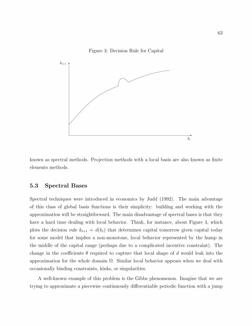
63

Figure 3: Decision Rule for CapitalFigure 1: Insert Title Here

kt+1

kt

1

known as spectral methods. Projection methods with a local basis are also known as finite

elements methods.

5.3 Spectral Bases

Spectral techniques were introduced in economics by Judd (1992). The main advantage

of this class of global basis functions is their simplicity: building and working with the

approximation will be straightforward. The main disadvantage of spectral bases is that they

have a hard time dealing with local behavior. Think, for instance, about Figure 3, which

plots the decision rule kt+1 = d(kt) that determines capital tomorrow given capital today

for some model that implies a non-monotone, local behavior represented by the hump in

the middle of the capital range (perhaps due to a complicated incentive constraint). The

change in the coefficients θ required to capture that local shape of d would leak into the

approximation for the whole domain Ω. Similar local behavior appears when we deal with

occasionally binding constraints, kinks, or singularities.

A well-known example of this problem is the Gibbs phenomenon. Imagine that we are

trying to approximate a piecewise continuously differentiable periodic function with a jump

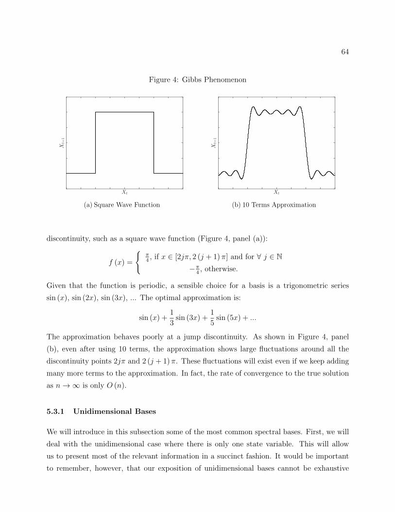
64

Figure 4: Gibbs PhenomenonFigure 1: Title

Xt

Xt+1

(a) Square Wave Function

Xt

Xt+1

(b) 10 Terms Approximation

1

discontinuity, such as a square wave function (Figure 4, panel (a)):

f (x) =

π4, if x ∈ [2jπ, 2 (j + 1) π] and for ∀ j ∈ N

−π4, otherwise.

Given that the function is periodic, a sensible choice for a basis is a trigonometric series

sin (x), sin (2x), sin (3x), ... The optimal approximation is:

sin (x) +1

3sin (3x) +

1

5sin (5x) + ...

The approximation behaves poorly at a jump discontinuity. As shown in Figure 4, panel

(b), even after using 10 terms, the approximation shows large fluctuations around all the

discontinuity points 2jπ and 2 (j + 1) π. These fluctuations will exist even if we keep adding

many more terms to the approximation. In fact, the rate of convergence to the true solution

as n→∞ is only O (n).

5.3.1 Unidimensional Bases

We will introduce in this subsection some of the most common spectral bases. First, we will

deal with the unidimensional case where there is only one state variable. This will allow

us to present most of the relevant information in a succinct fashion. It would be important

to remember, however, that our exposition of unidimensional bases cannot be exhaustive

65

(for instance, in the interest of space, we will skip splines) and that the researcher may

find herself tackling a problem that requires a specific basis. One of the great advantages

of projection methods is their flexibility to accommodate unexpected requirements. In the

next subsection, we will deal with the case of an arbitrary number of state variables and

we will discuss how to address the biggest challenge of projection methods: the curse of

dimensionality.

5.3.1.1 Monomials A first basis is the monomials 1, x, x2, x3, ... Monomials are simple

and intuitive. Furthermore, even if this basis is not composed by orthogonal functions, if

J1 is the space of bounded measurable functions on a compact set, the Stone-Weierstrass

theorem tells us that we can uniformly approximate any continuous function defined on a

closed interval with linear combinations of these monomials.

(Rudin, 1976, p. 162) provides a formal statement of the theorem:

Theorem 1 (Stone-Weierstrass). Let A be an algebra of real continuous functions on a

compact set K. If A separates points on K and if A vanishes at no point of K, then the

uniform closure B of A consists of all real continuous functions on K.

A consequence of this theorem is that if we have a real function f that is continuous on

K, we can find another function h ∈ B such that for ε > 0:

|f (x)− h (x)| < ε,

for all x ∈ K.

Unfortunately, monomials suffer from two severe problems. First, monomials are (nearly)

multicollinear. Figure 5 plots the graphs of x10 (continuous line) and x11 (discontinuous line)

for x ∈ [0.5, 1.5]. Both functions have a very similar shape. As we add higher monomials,

the new components of the solution do not allow the distance between the exact function we

want to approximate and the computed approximation to diminish sufficiently fast.18

18A sharp case of this problem is when H (·) is linear. In that situation, the solution of the projection

involves the inversion of matrices. When the basis functions are similar, the condition numbers of these

matrices (the ratio of the largest and smallest absolute eigenvalues) are too high. Just the first six mono-

mials can generate condition numbers of 1010. In fact, the matrix of the least squares problem of fitting a

polynomial of degree 6 to a function (the Hilbert Matrix ) is a popular test of numerical accuracy since it

maximizes rounding errors. The problem of the multicollinearity of monomials is also well appreciated in

econometrics.

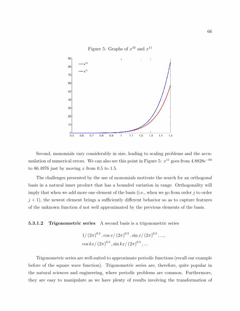
66

Figure 5: Graphs of x10 and x11

Second, monomials vary considerably in size, leading to scaling problems and the accu-

mulation of numerical errors. We can also see this point in Figure 5: x11 goes from 4.8828e−04

to 86.4976 just by moving x from 0.5 to 1.5.

The challenges presented by the use of monomials motivate the search for an orthogonal

basis in a natural inner product that has a bounded variation in range. Orthogonality will

imply that when we add more one element of the basis (i.e., when we go from order j to order

j + 1), the newest element brings a sufficiently different behavior so as to capture features

of the unknown function d not well approximated by the previous elements of the basis.

5.3.1.2 Trigonometric series A second basis is a trigonometric series

1/ (2π)0.5 , cosx/ (2π)0.5 , sinx/ (2π)0.5 , ...,

cos kx/ (2π)0.5 , sin kx/ (2π)0.5 , ...

Trigonometric series are well-suited to approximate periodic functions (recall our example

before of the square wave function). Trigonometric series are, therefore, quite popular in

the natural sciences and engineering, where periodic problems are common. Furthermore,

they are easy to manipulate as we have plenty of results involving the transformation of

67

trigonometric functions and we can bring to the table the powerful tools of Fourier analysis.

Sadly, economic problems are rarely periodic (except in the frequency analysis of time series)

and periodic approximations to non-periodic functions are highly inefficient.

5.3.1.3 Orthogonal polynomials of the Jacobi type We motivated before the need

to use a basis of orthogonal functions. Orthogonal polynomials of the Jacobi (also known as

hypergeometric) type are a flexible class of polynomials well-suited for our needs.

The Jacobi polynomial of degree n, Pα,βn (x) for α, β > −1, is defined by the orthogonality

condition: ∫ 1

−1

(1− x)α (1 + x)β Pα,βn (x)Pα,β

m (x) dx = 0 for m 6= n

One advantage of this class of polynomials is that we have a large number of alternative

expressions for them. The orthogonality condition implies, with the normalizations:

Pα,βn (1) =

(n+ α

n

),

that the general n term is given by:

2−nn∑k=0

(n+ α

k

)(n+ β

n− k

)(x− 1)n−k (x+ 1)k

Recursively:

2 (n+ 1) (n+ α + β + 1) (2n+ α + β)Pn+1 =((2n+ α + β + 1) (α2 − β2)

+ (2n+ α + β) (2n+ α + β + 1) (2n+ α + β + 2)x

)Pn

−2 (n+ α) (n+ β) (2n+ α + β + 2)Pn−1

Two important cases of Jacobi polynomials are the Legendre polynomials, where α =

β = −12, and the Chebyshev polynomials, where α = β = 0. There is a generalization of Leg-

endre and Chebyshev polynomials, still within the Jacobi family, known as the Gegenbauer

polynomials, which set α = β = υ − 12

for a parameter υ.

Boyd and Petschek (2014) compare the performance of Gegenbauer, Legendre, and

Chebyshev polynomials. Their Table 1 is particularly informative. We read it as suggest-

ing that, except for some exceptions that we find of less relevance in the solution of DSGE

68

models, Chebyshev polynomials are the most convenient of the three classes of polynomials.

Thus, from now on, we focus on Chebyshev polynomials.

5.3.1.4 Chebyshev polynomials Chebyshev polynomials are one of the most common

tools of applied mathematics. See, for example, Boyd (2000) and Fornberg (1996) for refer-

ences and background material. The popularity of Chebyshev polynomials is easily explained

if we consider some of their advantages.

First, numerous simple closed-form expressions for the Chebyshev polynomials are avail-

able. Thus, the researcher can easily move from one representation to another according to

her convenience. Second, the change between the coefficients of a Chebyshev expansion of

a function and the values of the function at the Chebyshev nodes is quickly performed by

the cosine transform. Third, Chebyshev polynomials are more robust than their alternatives

for interpolation. Fourth, Chebyshev polynomials are smooth and bounded between [−1, 1].

Finally, several theorems bound the errors for Chebyshev polynomials’ interpolations.

The most common definition of the Chebyshev polynomials is recursive, with T0 (x) = 1,

T1 (x) = x, and the general n+ 1-th order polynomial given by:

Tn+1 (x) = 2xTn (x)− Tn−1 (x)

Applying this recursive definition, the first few polynomials are 1, x, 2x2 − 1, 4x3 − 3x,

8x4 − 8x2 + 1,... Thus, the approximation of a function with Chebyshev polynomials is not

different from an approximation with monomials (and, thus, we can rely on appropriate

versions of the Stone-Weierstrass theorem), except that the orthogonality properties of how

Chebyshev polynomials group the monomials make the approximation better conditioned.

Figure 6 plots the Chebyshev polynomials of order 0 to 5. The first two polynomials

coincide with the first two monomials, a constant and the 45-degree line. The Chebyshev

polynomial of order two is a parabola. Higher-order Chebyshev polynomials accumulate

several waves. Figure 6 shows that the Chebyshev polynomials of order n has n zeros, given

by

xk = cos

(2k − 1

2nπ

), k = 1, ..., n.

This property will be useful when we describe collocation in a few pages. Also, these zeros

are quadratically clustered toward ±1.

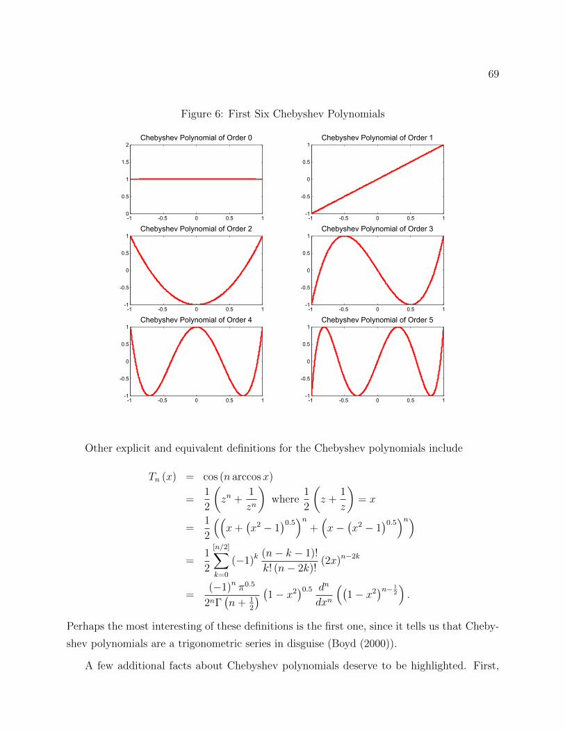
69

Figure 6: First Six Chebyshev Polynomials

-1 -0.5 0 0.5 10

0.5

1

1.5

2Chebyshev Polynomial of Order 0

-1 -0.5 0 0.5 1-1

-0.5

0

0.5

1Chebyshev Polynomial of Order 1

-1 -0.5 0 0.5 1-1

-0.5

0

0.5

1Chebyshev Polynomial of Order 2

-1 -0.5 0 0.5 1-1

-0.5

0

0.5

1Chebyshev Polynomial of Order 3

-1 -0.5 0 0.5 1-1

-0.5

0

0.5

1Chebyshev Polynomial of Order 4

-1 -0.5 0 0.5 1-1

-0.5

0

0.5

1Chebyshev Polynomial of Order 5

Other explicit and equivalent definitions for the Chebyshev polynomials include

Tn (x) = cos (n arccosx)

=1

2

(zn +

1

zn

)where

1

2

(z +

1

z

)= x

=1

2

((x+

(x2 − 1

)0.5)n

+(x−

(x2 − 1

)0.5)n)

=1

2

[n/2]∑k=0

(−1)k(n− k − 1)!

k! (n− 2k)!(2x)n−2k

=(−1)n π0.5

2nΓ(n+ 1

2

) (1− x2)0.5 dn

dxn

((1− x2

)n− 12

).

Perhaps the most interesting of these definitions is the first one, since it tells us that Cheby-

shev polynomials are a trigonometric series in disguise (Boyd (2000)).

A few additional facts about Chebyshev polynomials deserve to be highlighted. First,

70

the n+ 1 extrema of the polynomial Tn (xk) (n > 0) are given by:

xk = cos

(k

nπ

), k = 0, ..., n. (5.2)

All these extrema are either -1 or 1. Furthermore, two of the extrema are at the endpoints

of the domain: Tn (−1) = (−1)n and Tn (1) = 1. Second, the domain of the Chebyshev

polynomials is [−1, 1]. Since the domain of a state variable x in a DSGE model would be,

in general, different from [−1, 1], we can use a linear translation from [a, b] into [−1, 1] :

2x− ab− a − 1.

Third, the Chebyshev polynomials are orthogonal with respect to the weight function:

w (x) =1

(1− x2)0.5 .

We conclude the presentation of Chebyshev polynomials with two remarkable results,

which we will use below. The first result, due to Erdos and Turan (1937),19 tells us that if

an approximating function is exact at the roots of the nth1 order Chebyshev polynomial, then,

as n1 →∞, the approximation error becomes arbitrarily small. The Chebyshev interpolation

theorem will motivate, in a few pages, the use of orthogonal collocation where we pick as

collocation points the zeros of a Chebyshev polynomial (there are also related, less used,

results when the extrema of the polynomials are chosen instead of the zeros).

Theorem 2 (Chebyshev interpolation theorem). If d (x) ∈ C [a, b], if φi (x) , i = 0, ... is a

system of polynomials (where φi (x) is of exact degree i) orthogonal to with respect to w (x)

on [a, b] and if pj =∑j

i=0 θiφi (x) interpolates f (x) in the zeros of φn+1 (x), then:

limj→∞

(‖d− pj‖2

)2= lim

n→∞

∫ b

a

w (x) (d (x)− pj)2 dx = 0

We stated a version of the theorem that shows L2 convergence (a natural norm in eco-

nomics), but the result holds for Lp convergence for any p > 1. Even if we called this

result the Chebyshev interpolation theorem, its statement is more general, as it will apply to

other polynomials that satisfy an orthogonality condition. The reason we used Chebyshev

19We reproduce the statement of the theorem, with only minor notational changes, from Mason and

Handscomb (2003), chapter 3, where the interested reader can find related results and all the relevant

details. This class of theorems is usually derived in the context of interpolating functions.

71

in the theorem’s name is that the results are even stronger if the function d (x) satisfies a

Dini-Lipschitz condition and the polynomials φi (x) are Chebyshev to uniform convergence,

a much more reassuring finding.20

But the previous result requires that j → ∞, which is impossible in real applications.

The second result will give a sense of how big is the error we are accepting by truncating

the approximation of d (·) after a finite (and often relatively low) j.

Theorem 3 (Chebyshev truncation theorem, Boyd, 2000, p. 47). The error in approximat-

ing d is bounded by the sum of the absolute values of all the neglected coefficients. In other

words, if we have

dj ( ·| θ) =

j∑i=0

θiψi (·)

then ∣∣d (x)− dj (x| θ)∣∣ ≤ ∞∑

i=j+1

|θi|

for any x ∈ [−1, 1] and any j.

We can make the last result even stronger. Under certain technical conditions, we will

have a geometric convergence of the Chebyshev approximation to the exact unknown func-

tion.21 And when we have geometric convergence,∣∣d (x)− dj (x| θ)∣∣ ∼ O (θj)

that is, the truncation error created by stopping at the polynomial j is of the same order of

magnitude as the coefficient θj of the last polynomial. This result also provides us with a

20A function f satisfies a Dini-Lipschitz condition if

limδ→0+

ω (δ) log δ = 0

where ω (δ) is a modulus of continuity of f with respect to δ such that:

|f (x+ δ)− f (x)| ≤ ω (δ) .

21Convergence of the coefficients is geometric if

limj→∞

log (|θj |) /j = constant.

If the lim is infinity, convergence is supergeometric; if the lim is zero, convergence is subgeometric.

72

simple numerical test: we can check the coefficient θj from our approximation: if θj is not

close enough to zero, we probably need to increase j. We will revisit the evaluation of the

accuracy of an approximation in Section 7.

Remark 19 (Change of variables). We mentioned above that, since a state variable xt in

a DSGE model would have, in general, a domain different from [−1, 1], we can use a linear

translation from [a, b] into [−1, 1] :

2xt − ab− a − 1.

This transformation points to a more general idea: the change of variables as a way to

improve the accuracy of an approximation (see also Section 4.5 for the application of the

same idea in perturbation). Imagine that we are solving the stochastic neoclassical growth

model. Instead of searching for

ct = d1 (kt, zt)

and

kt+1 = d2 (kt, zt) ,

we could, instead, search for

log ct = d1 (log kt, zt)

and

log kt+1 = d2 (log kt, zt) ,

by defining

log ct = d1,j(

log kt, zt| θ1)

=

j∑i=0

θ1iψi (log kt, zt)

and

log kt+1 = d2,j(

log kt, zt| θ2)

=

j∑i=0

θ2iψi (log kt, zt) .

In fact, even in the basic projection example above, we already have a taste of this idea, as

we used zt as a state variable, despite the fact that it appears in the production function

as ezt . An alternative yet equivalent reparameterization writes At = ezt and zt = logAt.

The researcher can use her a priori knowledge of the model (or preliminary computational

results) to search for an appropriate change of variables in her problem. We have changed

both state and control variables, but nothing forced us to do so: we could have just changed

one variable but not the other or employed different changes of variables.

73

Remark 20 (Boyd’s moral principle). All of the conveniences of Chebyshev polynomials

we just presented are not just theoretical. Decades of real-life applications have repeatedly

shown how well Chebyshev polynomials work in a wide variety of applications. In the

case of DSGE models, the outstanding performance of Chebyshev polynomial has been

shown by Aruoba, Fernandez-Villaverde, and Rubio-Ramırez (2006) and Caldara, Fernandez-

Villaverde, Rubio-Ramırez, and Yao (2012). John Boyd (2000, p. 10), only half-jokingly,

has summarized these decades of experience in what he has named his Moral Principle 1:

1. When in doubt, use Chebyshev polynomials unless the solution is spatially periodic,

in which case an ordinary Fourier series is better.

2. Unless you are sure another set of basis functions is better, use Chebyshev polynomials.

3. Unless you are really, really sure another set of basis functions is better, use Chebyshev

polynomials.

5.3.2 Multidimensional Bases

All of the previous discussion presented unidimensional basis functions. This was useful to

introduce the topic. However, most problems in economics are multidimensional: nearly all

DSGE models involve several state variables. How do we generalize our basis functions?

The answer to this question is surprisingly important. Projection methods suffer from an

acute curse of dimensionality. While solving DSGE models with one or two state variables

and projection methods is relatively straightforward, solving DSGE models with 20 state

variables and projection methods is a challenging task due to the curse of dimensionality.

The key to tackling this class of problems is to intelligently select the multidimensional basis.

5.3.2.1 Discrete state variables The idea that the state variables are continuous was

implicit in our previous discussion. However, there are many DSGE models where either

some state variable is discrete (i.e., the government can be in default or not, as in Bocola

(2015), or monetary policy can be either active or passive in the sense of Leeper (1991)) or

where we can discretize one continuous state variable without losing much accuracy. The best

example of the latter is the discretization of exogenous stochastic processes for productivity

or preference shocks. Such discretization can be done with the procedures proposed by

74

Tauchen (1986) or Kopecky and Suen (2010), who find a finite state Markov chain that

generates the same population moments than the continuous process. Experience suggests

that, in most applications, a Markov chain with 5 or 7 states suffices to capture nearly all

the implications of the stochastic process for quantitative analysis.

A problem with discrete state variables can be thought of as one where we search for a

different decision rule for each value of that state variable. For instance, in the stochastic

neoclassical growth model with state variables kt and zt, we can discretize the productivity

level zt into a Markov chain with n points

zt ∈ z1, .., zn

and transition matrix:

Pz,z′ =

p11 . . . p1n

.... . .

...

pn1 . . . pnn

(5.3)

where entry pij is the probability that the chain will move from position i in the current

period to position j in the next period.

Remark 21 (Discretization methods). Tauchen (1986) procedure to discretize an AR(1)

stochastic process

zt = ρzt−1 + εt

with stationary distribution N(0, σ2z), where σz = σε√

1−ρ2, works as follows:

Algorithm 2 (AR(1) Discretization).

1. Set n, the number of potential realizations of the process z.

2. Set the upper (z) and lower (z) bounds for the process. An intuitive way to set the

bounds is to pick m such that:

z = mσz

z = −mσz

The latter alternative is appealing given the symmetry of the normal distribution

around 0. Usual values of m are between 2 and 3.

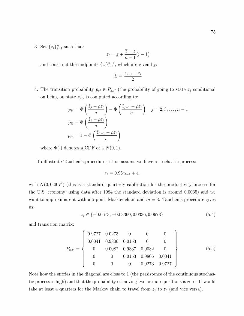
75

3. Set zini=1 such that:

zi = z +z − zn− 1

(i− 1)

and construct the midpoints zin−1i=1 , which are given by:

zi =zi+1 + zi

2

4. The transition probability pij ∈ Pz,z′ (the probability of going to state zj conditional

on being on state zi), is computed according to:

pij = Φ

(zj − ρzi

σ

)− Φ

(zj−1 − ρzi

σ

)j = 2, 3, . . . , n− 1

pi1 = Φ

(z1 − ρzi

σ

)pin = 1− Φ

(zn−1 − ρzi

σ

)where Φ(·) denotes a CDF of a N(0, 1).

To illustrate Tauchen’s procedure, let us assume we have a stochastic process:

zt = 0.95zt−1 + εt

with N(0, 0.0072) (this is a standard quarterly calibration for the productivity process for

the U.S. economy; using data after 1984 the standard deviation is around 0.0035) and we

want to approximate it with a 5-point Markov chain and m = 3. Tauchen’s procedure gives

us:

zt ∈ −0.0673,−0.03360, 0.0336, 0.0673 (5.4)

and transition matrix:

Pz,z′ =

0.9727 0.0273 0 0 0

0.0041 0.9806 0.0153 0 0

0 0.0082 0.9837 0.0082 0

0 0 0.0153 0.9806 0.0041

0 0 0 0.0273 0.9727

(5.5)

Note how the entries in the diagonal are close to 1 (the persistence of the continuous stochas-

tic process is high) and that the probability of moving two or more positions is zero. It would

take at least 4 quarters for the Markov chain to travel from z1 to z5 (and vice versa).

76

Tauchen’s procedure can be extended to VAR processes instead of an AR process. This

is convenient because we can always rewrite a general ARMA(p,q) process as a VAR(1) (and

a VAR(p) as a VAR(1)) by changing the definition of the state variables. Furthermore, open

source implementations of the procedure exist for all major programming languages.

Kopecky and Suen (2010) show that an alternative procedure proposed by Rouwenhorst

(1995) is superior to Tauchen’s method when ρ, the persistence of the stochastic process, is

close to 1. The steps of Rouwenhorst (1995)’s procedure are:

Algorithm 3 (Alternative AR(1) Discretization).

1. Set n, the number of potential realizations of the process z.

2. Set the upper (z) and lower (z) bounds for the process. Let z = −λ and z = λ. λ can

be set to be λ =√n− 1σz.

3. Set zini=1 such that:

zi = z +z − zn− 1

(i− 1)

4. When n = 2, let P2 be given by:

P2 =

[p 1− p

1− q q

]p, q can be set to be p = q = 1+ρ

2.

5. For n ≥ 3, construct recursively the transition matrix:

Pn = p

[Pn−1 0

0′ 0

]+ (1− p)

[0 Pn−1

0 0′

]+ (1− q)

[0′ 0

Pn−1 0

]+ q

[0 0′

0 Pn−1

]where 0 is an (n − 1) × 1 column vector of zeros. Divide all but the top and bottom

rows by 2 so that the sum of the elements of each row is equal to 1. The final outcome

is Pz,z′ .

Once productivity has been discretized, we can search for

c (k, zm) = dc,m,j (k| θm,c) =

j∑i=0

θm,ci ψi (k)

k (k, zm) = dk,m,j(k| θm,k

)=

j∑i=0

θm,ki ψi (k)

77

where m = 1, ..., n. That is, we search for decision rules for capital and consumption when

productivity is z1 today, decision rules for capital and consumption when productivity is z2

today, and so on, for a total of 2 × n decision rules. Since n is usually a small number (we

mentioned above 5 or 7), the complexity of the problem is not exploding.

Note that since we substitute these decision rules in the Euler equation:

u′ (ct) = βEt[u′ (ct+1)

(αezt+1kα−1

t+1 + 1− δ)]. (5.6)

to get:

u′(dc,m,j (k| θm,c)

)=

βn∑l=0

pml

[u′(dc,l,j

(dk,m,j

(k| θm,k

)∣∣ θl,c)) (αezt+1(dk,m,j

(k| θm,k

))α−1

t+1+ 1− δ

)]we are still taking account of the fact that productivity can change in the next period (and

hence, consumption and capital accumulation will be determined by the decision rule for

the next period level of productivity). Also, since now the stochastic process is discrete,

we can substitute the integral on the right-hand side of equation (5.6) for the much simpler

sum operator with the probabilities from the transition matrix (5.3). Otherwise, we would

need to use a quadrature method to evaluate the integral (see Judd (1998) for the relevant

formulae and the proposal in Judd, Maliar, and Maliar (2011a)).

Thus, discretization of state variables such as the productivity shock is more often than

not an excellent strategy to deal with multidimensional problems: simple, transparent, and

not too burdensome computationally. Furthermore, we can discretize some of the state vari-

ables and apply the methods in the next paragraphs to deal with the remaining continuous

state variables. In computation, mixing of strategies is often welcomed.

5.3.2.2 Tensors Tensors build multidimensional basis functions by finding the Kronecker

product of all unidimensional basis functions.22 Imagine, for example, that we have two state

variables, physical capital kt and human capital ht. We have three Chebyshev polynomials

for each of these two state variables:

ψk0 (kt) , ψk1 (kt) , and ψk2 (kt)

22One should not confuse the tensors presented here with the tensor notation used for perturbation meth-

ods. While both situations deal with closely related mathematical objects, the key when we were dealing

with perturbation was the convenience that tensor notation offered.

78

and

ψh0 (ht) , ψh1 (ht) , and ψh2 (ht) .

Then, the tensor is given by:

ψk0 (kt)ψh0 (ht) , ψk0 (kt)ψ

h1 (ht) , ψk0 (kt)ψ

h2 (ht) ,

ψk1 (kt)ψh0 (ht) , ψk1 (kt)ψ

h1 (ht) , ψk1 (kt)ψ

h2 (ht) ,

ψk2 (kt)ψh2 (ht) , ψk2 (kt)ψ

h1 (ht) , and ψk2 (kt)ψ

h2 (ht) .

More formally, imagine that we want to approximate a function of n state variables

d : [−1, 1]n → R with Chebyshev polynomial of degree j. We build the sum:

dj ( ·| θ) =

j∑i1=0

. . .

j∑in=0

θi1,...,inψ1i1

(·) ∗ . . . ∗ ψnin (·)

where ψκiκ is the Chebyshev polynomials of degree iκ on the state variable κ and θ is the vector

of coefficients θi1,...,in . To make the presentation concise, we have made three simplifying

assumptions. First, we are dealing with the case that d is one-dimensional. Second, we

are using the same number of Chebyshev polynomials for each state variable. Three, the

functions ψκiκ could be different from the Chebyshev polynomials and belong to any basis

we want (there can even be a different basis for each state variable). Eliminating these

simplifications is straightforward, but notationally cumbersome.

There are two main advantages of a tensor basis. First, it is trivial to build. Second, if

the one-dimensional basis is orthogonal, then the tensor basis is orthogonal in the product

norm. The main disadvantage is the exponential growth in the number of coefficients θi1,...,in :

(j + 1)n. In the example above, even using only three Chebyshev polynomials (i.e., j = 2)

for each of these two state variables, we end up having to solve for nine coefficients. This

curse of dimensionality is acute: with five state variables and three Chebyshev polynomials,

we end up with 243 coefficients. With ten Chebyshev polynomials, we end up with 100,000

coefficients.

5.3.2.3 Complete polynomials In practice, it is infeasible to use tensors when we are

dealing with models with more than 3 continuous state variables and a moderate j. A

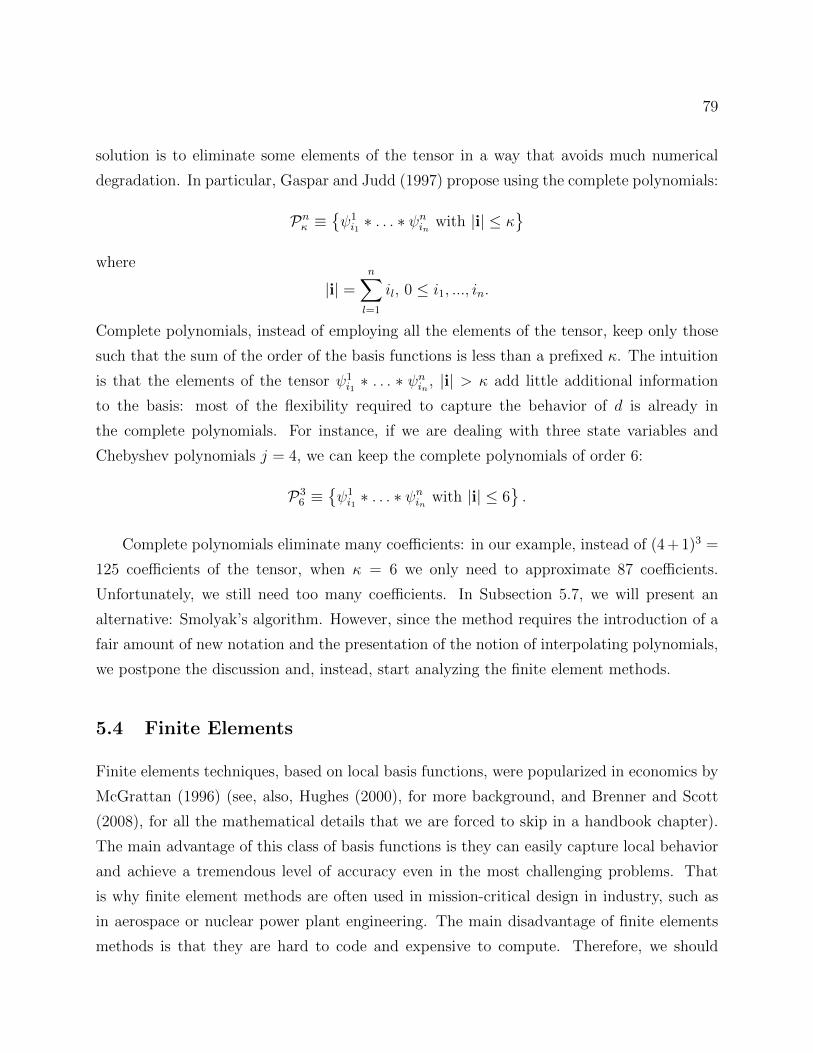
79

solution is to eliminate some elements of the tensor in a way that avoids much numerical

degradation. In particular, Gaspar and Judd (1997) propose using the complete polynomials:

Pnκ ≡ψ1i1∗ . . . ∗ ψnin with |i| ≤ κ

where

|i| =n∑l=1

il, 0 ≤ i1, ..., in.

Complete polynomials, instead of employing all the elements of the tensor, keep only those

such that the sum of the order of the basis functions is less than a prefixed κ. The intuition

is that the elements of the tensor ψ1i1∗ . . . ∗ ψnin , |i| > κ add little additional information

to the basis: most of the flexibility required to capture the behavior of d is already in

the complete polynomials. For instance, if we are dealing with three state variables and

Chebyshev polynomials j = 4, we can keep the complete polynomials of order 6:

P36 ≡

ψ1i1∗ . . . ∗ ψnin with |i| ≤ 6

.

Complete polynomials eliminate many coefficients: in our example, instead of (4 + 1)3 =

125 coefficients of the tensor, when κ = 6 we only need to approximate 87 coefficients.

Unfortunately, we still need too many coefficients. In Subsection 5.7, we will present an

alternative: Smolyak’s algorithm. However, since the method requires the introduction of a

fair amount of new notation and the presentation of the notion of interpolating polynomials,

we postpone the discussion and, instead, start analyzing the finite element methods.

5.4 Finite Elements

Finite elements techniques, based on local basis functions, were popularized in economics by

McGrattan (1996) (see, also, Hughes (2000), for more background, and Brenner and Scott

(2008), for all the mathematical details that we are forced to skip in a handbook chapter).

The main advantage of this class of basis functions is they can easily capture local behavior

and achieve a tremendous level of accuracy even in the most challenging problems. That

is why finite element methods are often used in mission-critical design in industry, such as

in aerospace or nuclear power plant engineering. The main disadvantage of finite elements

methods is that they are hard to code and expensive to compute. Therefore, we should

80

choose this strategy when accuracy is more important than speed of computation or when

we are dealing with complicated, irregular problems.

Finite elements start by bounding the domain Ω of the state variables. Some of the

bounds would be natural (i.e., kt > 0). Other bounds are not (kt < k) and we need some

care in picking them. For example, we can guess a k sufficiently large such that, in the

simulations of the model, kt never reaches k. This needs, however, to be verified and some

iterative fine-tuning may be required.23

The second step in the finite elements method is to partition Ω into small, non-intersecting

elements. These small sections are called elements (hence the name, “finite elements”). The

boundaries of the elements are called nodes. The researcher enjoys a fantastic laxity in se-

lecting the partition. One natural partition is to divide Ω into equal elements: simple and

direct. But elements can be of unequal size. More concretely, we can have small elements

in the areas of Ω where the economy will spend most of the time, while just a few large

elements will cover areas of Ω infrequently visited (these areas can be guessed based on the

theoretical properties of the model, or they can be verified by an iterative procedure of ele-

ment partition; we will come back to this point below). Or we can have small elements in

the areas of Ω where the function d (·) we are looking for changes quickly in shape, while we

reserve large elements for areas of Ω where the function d is close to linear. Thanks to this

flexibility in the element partition, we can handle kinks or constraints, which are harder to

tackle with spectral methods (or next to impossible to do with perturbation, as they violate

differentiability conditions).24

An illustration of such capability appears in Figure 7, where we plot the domain Ω of a

dynamic model of a firm with two state variables, bonds bt on the x-axis (values to the right

denote positive bond holdings by the firm and values to the left negative bond holdings),

and capital kt on the y-axis. The domain Ω does not include an area in the lower left corner,

of combinations of negative bond holdings (i.e., debt) and low capital. This area is excluded

because of a financial constraint: firms cannot take large amounts of debt when they do not

23Even if the simulation rarely reaches k, it may be useful to repeat the computation with a slightly higher

bound ωk, with ω > 1, to check that we still do not get to k. In some rare cases, the first simulation might

not have reached k because the approximation of the function d (·) precluded traveling into that region.24This flexibility in the definition of the elements is a main reason why finite elements methods are

appreciated in industry, where applications often do not conform to the regularity technical conditions

required by perturbation or spectral techniques.

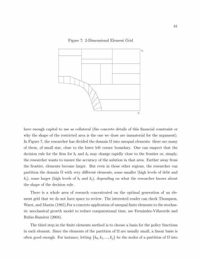
81

Figure 7: 2-Dimensional Element GridFigure 1: Insert Title Here

bt

kt

1

have enough capital to use as collateral (the concrete details of this financial constraint or

why the shape of the restricted area is the one we draw are immaterial for the argument).

In Figure 7, the researcher has divided the domain Ω into unequal elements: there are many

of them, of small size, close to the lower left corner boundary. One can suspect that the

decision rule for the firm for bt and kt may change rapidly close to the frontier or, simply,

the researcher wants to ensure the accuracy of the solution in that area. Farther away from

the frontier, elements become larger. But even in those other regions, the researcher can

partition the domain Ω with very different elements, some smaller (high levels of debt and

kt), some larger (high levels of bt and kt), depending on what the researcher knows about

the shape of the decision rule.

There is a whole area of research concentrated on the optimal generation of an ele-

ment grid that we do not have space to review. The interested reader can check Thompson,

Warsi, and Mastin (1985).For a concrete application of unequal finite elements to the stochas-

tic neoclassical growth model to reduce computational time, see Fernandez-Villaverde and

Rubio-Ramırez (2004).

The third step in the finite elements method is to choose a basis for the policy functions

in each element. Since the elements of the partition of Ω are usually small, a linear basis is

often good enough. For instance, letting k0, k1, ..., kj be the nodes of a partition of Ω into

82

Figure 8: Five Basis FunctionsFigure 1: Insert Title Here

kt+1

kt

1

elements, we can define the tent functions for i ∈ 1, j − 1

ψi (k) =

k−ki−1

ki−ki−1, if x ∈ [ki−1, ki]

ki+1−kki+1−ki , if k ∈ [ki, ki+1]

0 elsewhere

and the corresponding adjustments for the first function:

ψ0 (k) =

k0−kk1−k0 , if x ∈ [k0, k1]

0 elsewhere

and the last one

ψj (k) =

k−kj−1

kj−kj−1, if k ∈ [ki, ki+1]

0 elsewhere.

We plot examples of these tent functions in Figure 8.

We can extend this basis to higher dimensions by either discretizing some of the state

variables (as we did when we talked about spectral bases) or by building tensors of them.

Below, we will also see how to use Smolyak’s algorithm with finite elements.

The fourth step in the finite elements method is the same as for any other projection

method: we build

dn,j ( ·| θn) =

j∑i=0

θni ψi (·)

and we plug them into the operator H. Then, we find the unknown coefficients as we would

do with Chebyshev polynomials.

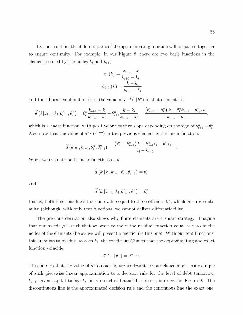
83

By construction, the different parts of the approximating function will be pasted together

to ensure continuity. For example, in our Figure 8, there are two basis functions in the

element defined by the nodes ki and ki+1

ψi (k) =ki+1 − kki+1 − ki

ψi+1 (k) =k − kiki+1 − ki

and their linear combination (i.e., the value of dn,j ( ·| θn) in that element) is:

d(k|ki+1, ki, θ

ni+1, θ

ni

)= θni

ki+1 − kki+1 − ki

+ θni+1

k − kiki+1 − ki

=

(θni+1 − θni

)k + θni ki+1 − θni+1ki

ki+1 − ki,

which is a linear function, with positive or negative slope depending on the sign of θni+1− θni .

Also note that the value of dn,j ( ·| θn) in the previous element is the linear function:

d(k|ki, ki−1, θ

ni , θ

ni−1

)=

(θni − θni−1

)k + θni−1ki − θni ki−1

ki − ki−1

.

When we evaluate both linear functions at ki

d(ki|ki, ki−1, θ

ni , θ

ni−1

)= θni

and

d(ki|ki+1, ki, θ

ni+1, θ

ni

)= θni

that is, both functions have the same value equal to the coefficient θni , which ensures conti-

nuity (although, with only tent functions, we cannot deliver differentiability).

The previous derivation also shows why finite elements are a smart strategy. Imagine

that our metric ρ is such that we want to make the residual function equal to zero in the

nodes of the elements (below we will present a metric like this one). With our tent functions,

this amounts to picking, at each ki, the coefficient θni such that the approximating and exact

function coincide:

dn,j ( ·| θn) = dn (·) .

This implies that the value of dn outside ki are irrelevant for our choice of θni . An example

of such piecewise linear approximation to a decision rule for the level of debt tomorrow,

bt+1, given capital today, kt, in a model of financial frictions, is drawn in Figure 9. The

discontinuous line is the approximated decision rule and the continuous line the exact one.

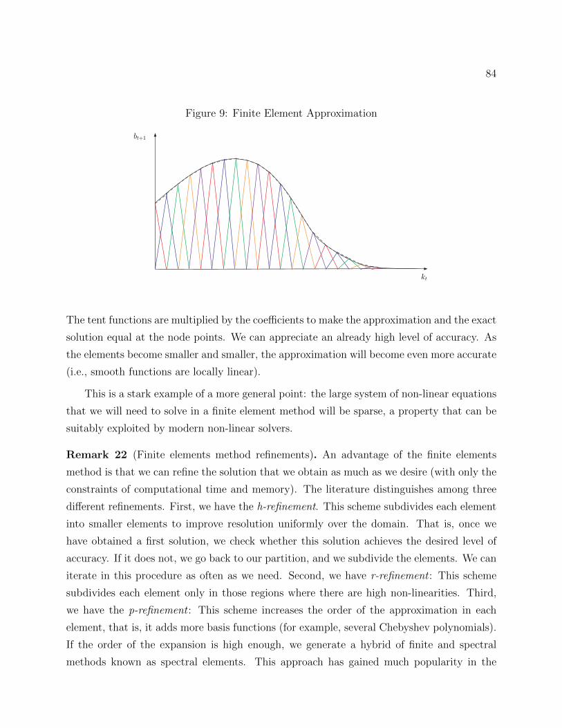
84

Figure 9: Finite Element ApproximationFigure 1: Insert Title Here

bt+1

kt

1

The tent functions are multiplied by the coefficients to make the approximation and the exact

solution equal at the node points. We can appreciate an already high level of accuracy. As

the elements become smaller and smaller, the approximation will become even more accurate

(i.e., smooth functions are locally linear).

This is a stark example of a more general point: the large system of non-linear equations

that we will need to solve in a finite element method will be sparse, a property that can be

suitably exploited by modern non-linear solvers.

Remark 22 (Finite elements method refinements). An advantage of the finite elements

method is that we can refine the solution that we obtain as much as we desire (with only the

constraints of computational time and memory). The literature distinguishes among three

different refinements. First, we have the h-refinement. This scheme subdivides each element

into smaller elements to improve resolution uniformly over the domain. That is, once we

have obtained a first solution, we check whether this solution achieves the desired level of

accuracy. If it does not, we go back to our partition, and we subdivide the elements. We can

iterate in this procedure as often as we need. Second, we have r-refinement : This scheme

subdivides each element only in those regions where there are high non-linearities. Third,

we have the p-refinement : This scheme increases the order of the approximation in each

element, that is, it adds more basis functions (for example, several Chebyshev polynomials).

If the order of the expansion is high enough, we generate a hybrid of finite and spectral

methods known as spectral elements. This approach has gained much popularity in the

85

natural sciences and engineering. See, for example, Solın, Segeth, and Dolezel (2004).

Sometimes, h-refinements and p-refinements are mixed in what is known as the hp-finite

element method, which delivers exponential convergence to the exact solution. Although

difficult to code and computationally expensive, an hp-finite element method is, perhaps,

the most powerful solution technique available for DSGE models, as it can tackle even the

most challenging problems.25

The three refinements can be automatically implemented: we can code the finite element

algorithm to identify the regions of Ω where, according to some goal of interest (for example,

how tightly a Euler equation is satisfied), we refine the approximation without further input

from the researcher. See Demkowicz (2007).

5.5 Objective Functions

Our second choice is to select a metric function ρ to determine how we “project.”The most

common answer to this question is given by a weighted residual : we select θ to get the

residual close to 0 in the weighted integral sense. Since we did not impose much structure on

the operator H and therefore, on the residual function R ( ·| θ), we will deal with the simplest

case where R ( ·| θ) is unidimensional. More general cases can be dealt with at the cost of

heavier notation. Given some weight functions φi : Ω→ R, we define the metric:

ρ (R ( ·| θ) , 0) =

0 if

∫Ωφi (x)R ( ·| θ) dx = 0, i = 1, .., j + 1

1 otherwise

Hence, the problem is to choose the θ that solves the system of integral equations:∫Ω

φi (x)R ( ·| θ) dx = 0, i = 1, .., j + 1. (5.7)

Note that, for the system to have a solution, we need j + 1 weight functions. Thanks to

the combination of approximating the function d by basis functions ψi and the definition of

weight functions φi, we have transformed a rather intractable functional equation problem

into a standard non-linear equations system. The solution of this system can be found using

25An additional, new refinement is the extended finite element method (x-fem), which adds to the ba-

sis discontinuous functions that can help in capturing irregularities in the solution. We are not aware of

applications of the x-fem in economics.

86

standard methods, such as a Newton algorithm for small problems or a Levenberg-Marquardt

method for bigger ones.

However, the system (5.7) may have no solution or it may have multiple ones. We know

very little about the theoretical properties of projection methods in economic applications.

The literature in applied mathematics was developed for the natural sciences and engineering

and many of the technical conditions required for existence and convergence theorems to work

do not easily travel across disciplines. In fact, some care must be put into ensuring that the

solution of the system (5.7) satisfies the transversality conditions of the DSGE model (i.e.,

we are picking the stable manifold). This can usually be achieved with the right choice of

an initial guess θ0 or by adding boundary conditions to the solver.

As was the case with the bases, we will have plenty of choices for our weight functions.

Instead of reviewing all possible alternatives, we will focus on the most popular ones in

economics.

5.5.1 Weight Function I: Least Squares

Least squares use as weight functions the derivatives of the residual function:

φi (x) =∂R (x| θ)∂θi−1

for all i ∈ 1, .., j + 1. This choice is motivated by the variational problem:

minθ

∫Ω

R2 ( ·| θ) dx

with first-order condition:∫Ω

∂R (x| θ)∂θi−1

R ( ·| θ) dx = 0, i = 1, .., j + 1.

This variational problem is mathematically equivalent to a standard regression problem in

econometrics.

While least squares are intuitive and there are algorithms that exploit some of their

structure to increase speed and decrease memory requirements, they require the computation

of the derivative of the residual, which can be costly. Also, least squares problems are often

ill-conditioned and complicated to solve numerically.

87

5.5.2 Weight Function II: Subdomain

The subdomain approach divides the domain Ω into 1, .., j+1 subdomains Ωi and define the

j + 1 step functions:

φi (x) =

1 if x ∈ Ωi

0 otherwise

This choice is equivalent to solving the system:∫Ωi

R ( ·| θ) dx = 0, i = 1, .., j + 1.

The researcher has plenty of flexibility to pick her subdomains as to satisfy her criteria of

interest.

5.5.3 Weight Function III: Collocation

This method is also known as pseudospectral or the method of selected points. It defines

the weight function as:

φi (x) = δ (x− xi)

where δ is the dirac delta function and xi are the j + 1 collocation points selected by the

researcher.

This method implies that the residual function is zero at the n collocation points. Thus,

instead of having to compute complicated integrals, we only need to solve the system:

R (xi| θ) = 0, i = 1, .., j + 1.

This is attractive when the operator H generates large non-linearities.

A systematic way to pick collocation points is to use the zeros of the (j + 1)th-order

Chebyshev polynomial in each dimension of the state variable (or the corresponding polyno-

mials, if we are using different approximation orders along each dimension). This approach

is known as orthogonal collocation. The Chebyshev interpolation theorem tells us that, with

this choice of collocation points, we can achieve Lp convergence and sometimes even uni-

form convergence to the unknown function d. Another possibility is to pick, as collocation

points, the extrema of the jth-order Chebyshev polynomial in each dimension. Experience

shows a surprisingly good performance of orthogonal collocation methods and it is one of

our recommended approaches.

88

5.5.4 Weight Function IV: Galerkin or Rayleigh-Ritz

The last weight function we consider is the Galerkin (also called Rayleigh-Ritz when it

satisfies some additional properties of less importance for economists). This approach takes

as the weight function the basis functions used in the approximation:

φi (x) = ψi−1 (x) .

Then we have: ∫Ω

ψi (x)R ( ·| θ) dx = 0, i = 1, .., j + 1.

The interpretation is that the residual has to be orthogonal to each of the basis functions.

The Galerkin approach is highly accurate and robust, but difficult to code. If the basis

functions are complete over J1 (they are indeed a basis of the space), then the Galerkin

solution will converge pointwise to the true solution as n goes to infinity:

limj→∞

dj ( ·| θ) = d (·)

Also, practical experience suggests that a Galerkin approximation of order j is as accurate

as a pseudospectral j + 1 or j + 2 expansion.

In the next two remarks, we provide some hints for a faster and more robust solution of

the system of non-linear equations:∫Ω

φi (x)R ( ·| θ) dx = 0, i = 1, .., j + 1, (5.8)

a task that can be difficult if the number of coefficients is large and the researcher does not

have a good initial guess θ0 for the solver.

Remark 23 (Transformations of the problem). A bottleneck for the solution of (5.7) can be

the presence of strong non-linearities. Fortunately, it is often the case that simple changes

in the problem can reduce these non-linearities. For example, Judd (1992) proposes that if

we have an Euler equation:1

ct= βEt

1

ct+1

Rt+1

where Rt+1 is the gross return rate of capital, we can take its inverse:

βct =

(Et

1

ct+1

Rt+1

)−1

,

89

which now is linear on the left-hand side and much closer to linear on the right-hand side.

Thus, instead of computing the residual for some state variable xt

R ( ·| θ) =1

c (xt| θ)− βEt

1

c (xt| θ)Rt+1 (xt| θ)

,

we compute:

R ( ·| θ) = βc (xt| θ)−(Et

1

c (xt| θ)Rt+1 (xt| θ)

)−1

.

Similar algebraic manipulations are possible in many DSGE models.

Remark 24 (Multistep schemes). The system (5.7) can involve a large number of coeffi-

cients. A natural strategy is to solve first a smaller system and to use that solution as an

input for a larger system. This strategy, called a multistep scheme, often delivers excellent

results, in particular when dealing with orthogonal bases such as Chebyshev polynomials.

More concretely, instead of solving the system for an approximation with j + 1 basis

functions, we can start by solving the system with only j′ + 1 j + 1 basis functions

and use the solution to this first problem as a guess for the more complicated problem. For

example, if we are searching for a solution with 10 Chebyshev polynomials and m dimensions,

we first find the approximation with only 3 Chebyshev polynomials. Therefore, instead of

solving a system of 10×m equations, we solve a system of 3×m. Once we have the solution

θ3, we build the initial guess for the problem with 10 Chebyshev polynomials as:

θ0 =[θ3,01×m, ...,01×m

],

that is, we use θ3 for the first coefficients and zero for the additional new coefficients. Since

the additional polynomials are orthogonal to the previous ones, the final values of the coef-

ficients associated with the three first polynomials will change little with the addition of 7

more polynomials: the initial guess θ3 is, thus, most splendid. Also, given the fast conver-

gence of Chebyshev polynomials, the coefficients associated with higher-order polynomials

will be close to zero. Therefore, our initial guess for those coefficients is also informative.

The researcher can use as many steps as she needs. By judiciously coding the projection

solver, the researcher can write the program as depending on an abstract number of Cheby-

shev polynomials. Then, she can call the solver inside a loop and iteratively increase the

level of approximation from j′ to j as slow or as fast as required.

90

5.6 A Worked-Out Example

We present now a worked-out example of how to implement a projection method in a DSGE

model. In particular, we will use Chebyshev polynomials and orthogonal collocation to solve

the stochastic neoclassical growth model with endogenous labor supply.

In this economy, there is a representative household, whose preferences over consumption,

ct, and leisure, 1− lt, are representable by the utility function:

E0

∞∑t=1

βt−1

(cτt (1− lt)1−τ)1−η

1− η

where β ∈ (0, 1) is the discount factor, η controls the elasticity of intertemporal substitution

and risk aversion, τ controls labor supply, and E0 is the conditional expectation operator.

There is one good in the economy, produced according to the aggregate production

function:

yt = eztkαt l1−αt

where kt is the aggregate capital stock, lt is aggregate labor, and zt is a stochastic process

for technology:

zt = ρzt−1 + εt

with |ρ| < 1 and εt ∼ N(0, σ2). Capital evolves according to:

kt+1 = (1− δ)kt + it

and the economy must satisfy the resource constraint yt = ct + it.

Since both welfare theorems hold in this economy, we solve directly for the social planner’s

problem:

V (kt, zt) = maxct,lt

(cτt (1− lt)1−τ)1−η

1− η + βEtV (kt+1, zt+1)

s.t. kt+1 = eztkαt l1−αt + (1− δ)kt − ct

zt = ρzt−1 + εt

given some initial conditions k0 and z0. Tackling the social planner’s problem is only done

for convenience, and we could also solve for the competitive equilibrium. In fact, one key

advantage of projection methods is that they easily handle non-Pareto efficient economies.

91

Table 2: Calibration

Parameter Value

β 0.991

η 5.000

τ 0.357

α 0.300

δ .0196

ρ 0.950

σ 0.007

We calibrate the model with standard parameter values to match U.S. quarterly data

(see Table 2). The only exception is η, for which we pick a value of 5, in the higher range of

empirical estimates. Such high-risk aversion induces, through precautionary behavior, more

curvature in the decision rules. This curvature would present a more challenging test bed

for the projection method.

We discretize zt into a 5-point Markov chain z1, ..., z5 using Tauchen’s procedure and

covering ±3 unconditional standard deviations of zt (this is the same Markov chain as the

example in Remark 21, see (5.4) and (5.5) for the concrete values of the discretization). We

will use pmn to denote the generic entry of the transition matrix Pz,z′ generated by Tauchen’s

procedure for zm today moving to zn next period.

Then, we approximate the value function V j (kt) and the decision rule for labor, lj (kt),

for j = 1, ..., 5 using 11 Chebyshev polynomials as:

V j(kt|θV,j

)=

10∑i=0

θV,ji Ti (kt) (5.9)

lj(kt|θl,j

)=

10∑i=0

θl,ki Ti (kt) (5.10)

Once we have the decision rule for labor, we can find output:

yj (kt) = eztkαt(lj(kt|θl,j

))1−α,

92

With output, from the first-order condition that relates the marginal utility consumption

and the marginal productivity of labor, we can find consumption:

cj (kt) =τ

1− τ (1− α)eztkαt(lj(kt|θl,j

))−α (1− lj

(kt|θl,j

))(5.11)

and, from the resource constraint, capital next period:

kj (kt) = eztkαt(lj(kt|θl,j

))1−α+ (1− δ)kt − cj (kt) (5.12)

Our notations yj (kt), cj (kt), and kj (kt) emphasize the exact dependence of these three

variables on capital and the productivity level: once we have approximated lj(kt|θl,j

), simple

algebra with the equilibrium conditions allows us to avoid further approximation.

We decided to approximate the value function and the decision rule for labor and use

them to derive the other variables of interest to illustrate how flexible projection methods

are. We could, as well, have decided to approximate the decision rules for consumption

and capital and find labor and the value function using the equilibrium conditions. The

researcher should pick the approximating functions that are more convenient, either for

algebraic reasons or her particular goals.

To solve for the unknown coefficients θV and θl, we plug the functions (5.9), (5.10),

(5.11), and (5.12) into the Bellman equation to get:

10∑i=0

θV,ji Ti (kt) =

((cj (kt))

θ (1−∑10

i=0 θliTi (kt)

)1−θ)1−τ

1− τ + β5∑

m=1

pjm

10∑i=0

θV,ji Ti(kj (kt)

)(5.13)

where, since we are already using the optimal decision rules, we can drop the max operator.

Also, we have substituted the expectation by the sum operator and the transition probabili-

ties pjm. We plug the same functions (5.9), (5.10), (5.11), and (5.12) into the Euler equation

to get: (cθt

(1−∑10

i=0 θl,ki Ti (kt)

)1−θ)1−τ

ct= βEt

5∑m=1

pjm

10∑i=0

θV,ji Ti(kj (kt)

)′, (5.14)

where Ti (kj (kt))

′is the derivative of the Chebyshev polynomial with respect to its argument.

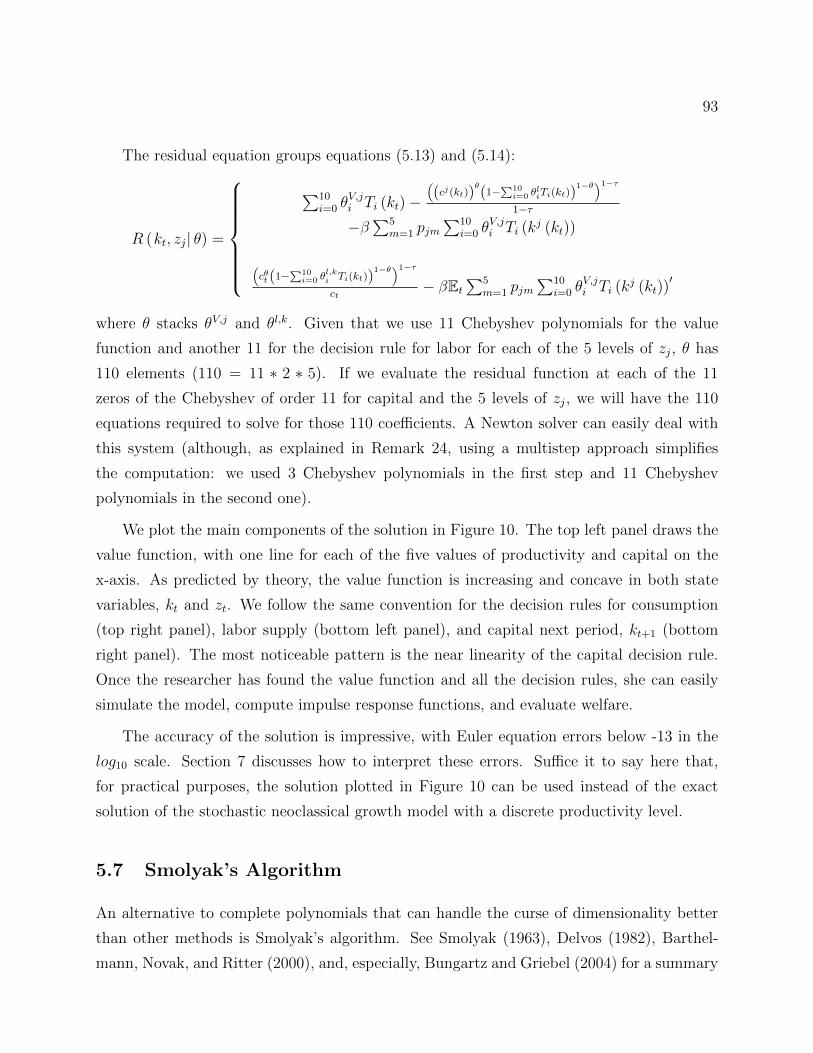
93

The residual equation groups equations (5.13) and (5.14):

R (kt, zj| θ) =

∑10i=0 θ

V,ji Ti (kt)−

((cj(kt))

θ(1−

∑10i=0 θ

liTi(kt))

1−θ)1−τ1−τ

−β∑5m=1 pjm

∑10i=0 θ

V,ji Ti (k

j (kt))

(cθt (1−

∑10i=0 θ

l,ki Ti(kt))

1−θ)1−τct

− βEt∑5

m=1 pjm∑10

i=0 θV,ji Ti (k

j (kt))′

where θ stacks θV,j and θl,k. Given that we use 11 Chebyshev polynomials for the value

function and another 11 for the decision rule for labor for each of the 5 levels of zj, θ has

110 elements (110 = 11 ∗ 2 ∗ 5). If we evaluate the residual function at each of the 11

zeros of the Chebyshev of order 11 for capital and the 5 levels of zj, we will have the 110

equations required to solve for those 110 coefficients. A Newton solver can easily deal with

this system (although, as explained in Remark 24, using a multistep approach simplifies

the computation: we used 3 Chebyshev polynomials in the first step and 11 Chebyshev

polynomials in the second one).

We plot the main components of the solution in Figure 10. The top left panel draws the

value function, with one line for each of the five values of productivity and capital on the

x-axis. As predicted by theory, the value function is increasing and concave in both state

variables, kt and zt. We follow the same convention for the decision rules for consumption

(top right panel), labor supply (bottom left panel), and capital next period, kt+1 (bottom

right panel). The most noticeable pattern is the near linearity of the capital decision rule.

Once the researcher has found the value function and all the decision rules, she can easily

simulate the model, compute impulse response functions, and evaluate welfare.

The accuracy of the solution is impressive, with Euler equation errors below -13 in the

log10 scale. Section 7 discusses how to interpret these errors. Suffice it to say here that,

for practical purposes, the solution plotted in Figure 10 can be used instead of the exact

solution of the stochastic neoclassical growth model with a discrete productivity level.

5.7 Smolyak’s Algorithm

An alternative to complete polynomials that can handle the curse of dimensionality better

than other methods is Smolyak’s algorithm. See Smolyak (1963), Delvos (1982), Barthel-

mann, Novak, and Ritter (2000), and, especially, Bungartz and Griebel (2004) for a summary

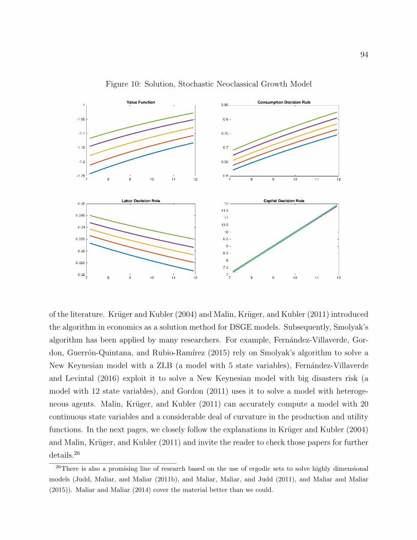
94

Figure 10: Solution, Stochastic Neoclassical Growth Model

of the literature. Kruger and Kubler (2004) and Malin, Kruger, and Kubler (2011) introduced

the algorithm in economics as a solution method for DSGE models. Subsequently, Smolyak’s

algorithm has been applied by many researchers. For example, Fernandez-Villaverde, Gor-

don, Guerron-Quintana, and Rubio-Ramırez (2015) rely on Smolyak’s algorithm to solve a

New Keynesian model with a ZLB (a model with 5 state variables), Fernandez-Villaverde

and Levintal (2016) exploit it to solve a New Keynesian model with big disasters risk (a

model with 12 state variables), and Gordon (2011) uses it to solve a model with heteroge-

neous agents. Malin, Kruger, and Kubler (2011) can accurately compute a model with 20

continuous state variables and a considerable deal of curvature in the production and utility

functions. In the next pages, we closely follow the explanations in Kruger and Kubler (2004)

and Malin, Kruger, and Kubler (2011) and invite the reader to check those papers for further

details.26

26There is also a promising line of research based on the use of ergodic sets to solve highly dimensional

models (Judd, Maliar, and Maliar (2011b), and Maliar, Maliar, and Judd (2011), and Maliar and Maliar

(2015)). Maliar and Maliar (2014) cover the material better than we could.

95

As before, we want to approximate a function (decision rule, value function, expectation,

etc.) on n state variables, d : [−1, 1]n → R (the generalization to the case d : [−1, 1]n → Rm

is straightforward, but tedious). The idea of Smolyak’s algorithm is to find a grid of points

G(q, n) ∈ [−1, 1]n where q > n and an approximating function d(x|θ,q, n) : [−1, 1]n → Rindexed by some coefficients θ such that, at the points xi ∈ G(q, n), the unknown function

d (·) and d(·|θ,q, n) are equal:

d (xi) = d(xi|θ,q, n)

and, at the points xi /∈ G(q, n), d(·|θ,q, n) is close to the unknown function d (·). In other

words, at the points xi ∈ G(q, n), the operator H (·) would be exactly satisfied and, at other

points, the residual function would be close to zero.

The challenge is to judiciously select grid points G(q, n) in such a way that the number

of coefficients θ does not explode with n. Smolyak’s algorithm is (almost) optimal for that

task within the set of polynomial approximations (Barthelmann, Novak, and Ritter (2000)).

Also, the method is universal, that is, almost optimal for many different function spaces.

5.7.1 Implementing Smolyak’s Algorithm

Our search of a grid of points G(q, n) and a function d(x|θ,q, n) will proceed in several steps.

5.7.1.1 First step: Transform the domain of the state variables For any state

variable xl, l = 1, ..., n that has a domain [a, b], we use a linear translation from [a, b] into

[−1, 1] :

xl = 2xl − ab− a − 1.

5.7.1.2 Second step: Setting the order of the polynomial We define m1 = 1 and

mi = 2i−1 + 1, i = 2, ..., where mi − 1 will be the order of the polynomial that we will use

to approximate d (·).

5.7.1.3 Third step: Building the Gauss–Lobotto nodes We build the sets:

Gi = ζ i1, ..., ζ imi ⊂ [−1, 1]

96

that contain the Gauss–Lobotto nodes (also known as the Clenshaw–Curtis points), that is,

the extrema of the Chebyshev polynomials:

ζ ij = −cos(j − 1

mi − 1π

), j = 1, ...,mi

with the initial set G1 = 0 (with a change of notation, this formula for the extrema is the

same as the one in equation (5.2)). For instance, the first three sets are given by:

G1 = 0, where i = 1,m1 = 1.

G2 = −1, 0, 1, where i = 2,m3 = 3.

G3 =

−1,− cos

(π4

), 0,− cos

(3π

4

), 1

, where i = 3,m5 = 5.

Since, in the construction of the sets, we impose that mi = 2i−1 +1, we generate sets that are

nested, that is, Gi ⊂ Gi+1, ∀i = 1, 2, . . .This result is crucial for the success of the algorithm.

5.7.1.4 Fourth step: building a sparse grid For any integer q bigger than the number

of state variables n, q > n, we define a sparse grid as the union of the Cartesian products:

G(q, n) =⋃

q−n+1≤|i|≤q

(Gi1 × ...× Gin),

where |i| = ∑nl=1 il. The integer q indexes the size of the grid and, with it, the precision of

the approximation.

To illustrate how this sparse grid works, imagine that we are dealing with a DSGE model

with two continuous state variables. If we pick q = 2 + 1 = 3, we have the sparse grid

G (3, 2) =⋃

2≤|i|≤3

(Gi1 × Gi2)

=(G1 × G1

)∪(G1 × G2

)∪(G2 × G1

)= (−1, 0) , (0, 1) , (0, 0) , (0,−1) , (1, 0)

We plot this grid in the top left panel of Figure 11, which reproduces Figure 1 in Kruger

and Kubler (2004).

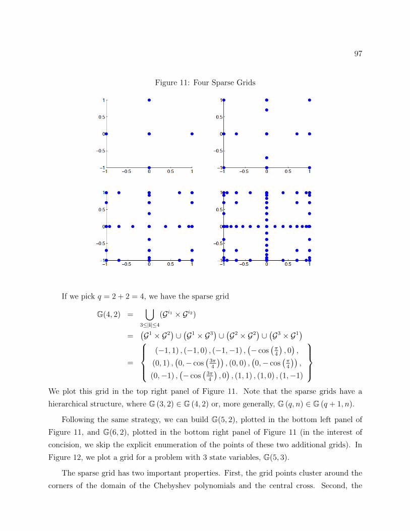
97

Figure 11: Four Sparse Grids

If we pick q = 2 + 2 = 4, we have the sparse grid

G(4, 2) =⋃

3≤|i|≤4

(Gi1 × Gi2)

=(G1 × G2

)∪(G1 × G3

)∪(G2 × G2

)∪(G3 × G1

)=

(−1, 1) , (−1, 0) , (−1,−1) ,

(− cos

(π4

), 0),

(0, 1) ,(0,− cos

(3π4

)), (0, 0) ,

(0,− cos

(π4

)),

(0,−1) ,(− cos

(3π4

), 0), (1, 1) , (1, 0) , (1,−1)

We plot this grid in the top right panel of Figure 11. Note that the sparse grids have a

hierarchical structure, where G (3, 2) ∈ G (4, 2) or, more generally, G (q, n) ∈ G (q + 1, n).

Following the same strategy, we can build G(5, 2), plotted in the bottom left panel of

Figure 11, and G(6, 2), plotted in the bottom right panel of Figure 11 (in the interest of

concision, we skip the explicit enumeration of the points of these two additional grids). In

Figure 12, we plot a grid for a problem with 3 state variables, G(5, 3).

The sparse grid has two important properties. First, the grid points cluster around the

corners of the domain of the Chebyshev polynomials and the central cross. Second, the

98

Figure 12: A Sparse Grid, 3 State Variables

number of points in a sparse grid when q = n + 2 is given by 1 + 4n + 2n(n − 1). The

cardinality of this grid grows polynomially on n2. Similar formulae hold for other q > n.

For example, the cardinality of the grid grows polynomially on n3 when q = n + 3. In fact,

the computational burden of the method notably increases as we keep n fixed and a rise q.

Fortunately, experience suggests that q = n+ 2 and q = n+ 3 are usually enough to deliver

the desired accuracy in DSGE models.

The nestedness of the sets of the Gauss–Lobotto nodes plays a central role in controlling

the cardinality of G(q, n). In comparison, the number of points in a rectangular grid is

5n, an integer that grows exponentially on n. If n = 2, this would correspond, in the top

right panel of Figure 11, to having all possible tensors of −1,− cos(π4

), 0,− cos

(3π4

), 1

and −1,− cos(π4

), 0,− cos

(3π4

), 1 covering the whole of the [−1, 1]2 square. Instead of

keeping these 25 points, Smolyak’s algorithm eliminates 12 of them and only keeps 13. To

illustrate how dramatic is the difference between polynomial and exponential growth, Table

3 shows the cardinality of both grids as we move from 2 state variables to 12.

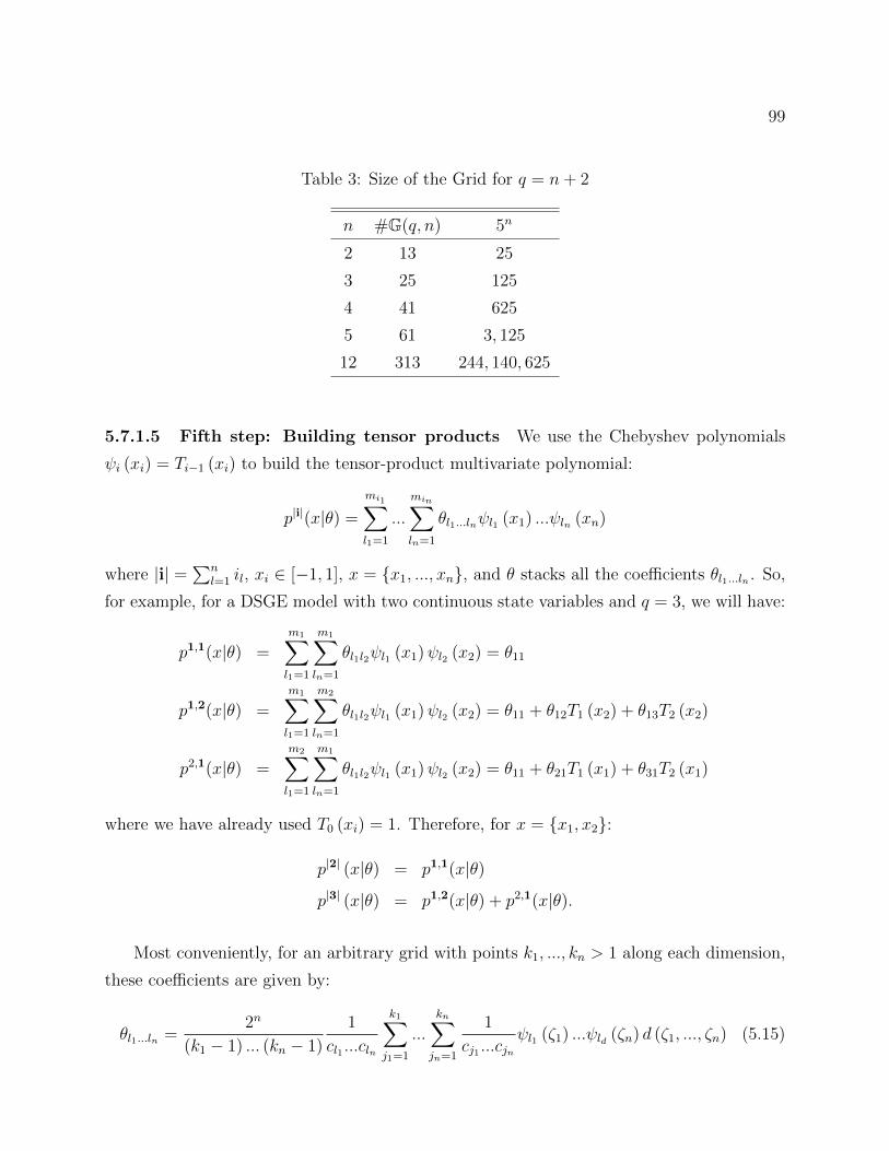
99

Table 3: Size of the Grid for q = n+ 2

n #G(q, n) 5n

2 13 25

3 25 125

4 41 625

5 61 3, 125

12 313 244, 140, 625

5.7.1.5 Fifth step: Building tensor products We use the Chebyshev polynomials

ψi (xi) = Ti−1 (xi) to build the tensor-product multivariate polynomial:

p|i|(x|θ) =

mi1∑l1=1

...

min∑ln=1

θl1...lnψl1 (x1) ...ψln (xn)

where |i| = ∑nl=1 il, xi ∈ [−1, 1], x = x1, ..., xn, and θ stacks all the coefficients θl1...ln . So,

for example, for a DSGE model with two continuous state variables and q = 3, we will have:

p1,1(x|θ) =

m1∑l1=1

m1∑ln=1

θl1l2ψl1 (x1)ψl2 (x2) = θ11

p1,2(x|θ) =

m1∑l1=1

m2∑ln=1

θl1l2ψl1 (x1)ψl2 (x2) = θ11 + θ12T1 (x2) + θ13T2 (x2)

p2,1(x|θ) =

m2∑l1=1

m1∑ln=1

θl1l2ψl1 (x1)ψl2 (x2) = θ11 + θ21T1 (x1) + θ31T2 (x1)

where we have already used T0 (xi) = 1. Therefore, for x = x1, x2:

p|2| (x|θ) = p1,1(x|θ)p|3| (x|θ) = p1,2(x|θ) + p2,1(x|θ).

Most conveniently, for an arbitrary grid with points k1, ..., kn > 1 along each dimension,

these coefficients are given by:

θl1...ln =2n

(k1 − 1) ... (kn − 1)

1

cl1 ...cln

k1∑j1=1

...

kn∑jn=1

1

cj1 ...cjnψl1 (ζ1) ...ψld (ζn) d (ζ1, ..., ζn) (5.15)

100

where cj = 1 for all j, except for the cases c1 = ckd = 2, and ζk ∈ Gi are the Gauss–Lobotto

nodes. This approximation is exact in the Gauss–Lobotto nodes and interpolates among

them.

There is nothing special about the use of Chebyshev polynomials as the basis functions

ψj (x) and we could rely, if required, on other basis functions. For instance, one can imple-

ment a finite element method with the Smolyak algorithm by partitioning Ω into elements

and defining local basis functions as in Nobile, Tempone, and Webster (2008).

5.7.1.6 Sixth step: Building the interpolating function in n dimensions The

Smolyak function that interpolates on G(q, n) is:

d(x|θ,q, n) =∑

max(n,q−n+1)≤|i|≤q

(−1)q−|i|

(n− 1

q − |i|

)p|i|(x|θ),

which is nothing more than the weighted sum of the tensors. In our previous example, a

DSGE model with two continuous state variables and q = 3, we will have the sparse grid:

G(3, 2) = (−1, 0) , (0, 1) , (0, 0) , (0,−1) , (1, 0)

(this sparse grid was drawn in the top left panel of Figure 11) and:

d(x|θ,q, n) =∑

2≤|i|≤3

(−1)3−|i|

(1

3− |i|

)p|i|(x|θ)

= (−1)

(1

1

)p|2|(x|θ) + (−1)0

(1

0

)p|3|(x|θ)

= p1,2(x|θ) + p2,1(x|θ)− p1,1(x|θ)= θ11 + θ21T1 (x1) + θ31T2 (x1) + θ12T1 (x2) + θ13T2 (x2) .

Each of the coefficients in this approximation is given by the formula in equation (5.15):

θ21 =1

2(d (1, 0)− d (−1, 0))

θ12 =1

2(d (0, 1)− d (0,−1))

θ31 =1

4(d (1, 0) + d (−1, 0))− 1

2d (0, 0)

θ13 =1

4(d (0, 1) + d (0,−1))− 1

2d (0, 0)

101

except the constant term:

θ11 =1

4(d (0, 1) + d (0,−1) + d (1, 0) + d (−1, 0)) ,

which instead ensures that the interpolating function satisfies d (0, 0) = d(x|θ,q, n). It is easy

to check that we indeed satisfy the condition that the approximating function equates the

unknown function at the points of the sparse grid. For example, at (−1, 0):

d((−1, 0) |θ,q, n) = θ11 + θ21T1 (−1) + θ31T2 (−1) + θ12T1 (0) + θ13T2 (0)

= θ11 − θ21 + θ31 − θ13

=1

4(d (0, 1) + d (0,−1) + d (1, 0) + d (−1, 0))

−1

2(d (1, 0)− d (−1, 0))

+1

4(d (1, 0) + d (−1, 0))− 1

2d (0, 0)

−1

4(d (0, 1) + d (0,−1)) +

1

2d (0, 0)

= d (−1, 0) .

An interesting property of this construction of d(x|θ,q, n) is that the cardinality of G(q, n)

and the number of coefficients on θ coincide. In our previous example, #G(3, 2) = 5 and

θ = θ11, θ21, θ31, θ12, θ13. A second relevant property is that d(x|θ,q, n) exactly replicates

any polynomial function built with monomials of degree less than or equal to q − n.

5.7.1.7 Seventh step: Solving for the polynomial coefficients We plug d(x|θ,q, n)

into the operator H (·) for all xi ∈ G(q, n). At this point the operator needs to be exactly

zero:

H (d(xi|θ,q, n)) = 0

and we solve for the unknown coefficients on θ. In our previous example, we had G(3, 2) =

(−1, 0) , (0, 1) , (0, 0) , (0,−1) , (1, 0) and, therefore:

d((−1, 0) |θ,q, n) = θ11 + θ21T1 (−1) + θ31T2 (−1) + θ12T1 (0) + θ13T2 (0) = θ11 − θ21 + θ31 − θ13

d((0, 1) |θ,q, n) = θ11 + θ21T1 (0) + θ31T2 (0) + θ12T1 (1) + θ13T2 (1) = θ11 − θ31 + θ12 + θ13

d((0, 0) |θ,q, n) = θ11 + θ21T1 (0) + θ31T2 (0) + θ12T1 (0) + θ13T2 (0) = θ11 − θ31 − θ13

d((0,−1) |θ,q, n) = θ11 + θ21T1 (0) + θ31T2 (0) + θ12T1 (−1) + θ13T2 (−1) = θ11 − θ31 − θ12 + θ13

d((1, 0) |θ,q, n) = θ11 + θ21T1 (1) + θ31T2 (1) + θ12T1 (0) + θ13T2 (0) = θ11 + θ21 + θ31 − θ13

102

The system of equations:

H (d(xi|θ,q, n)) = 0, xi ∈ G(q, n)

can be solved with a standard non-linear solver. Kruger and Kubler (2004) and Malin,

Kruger, and Kubler (2011) suggest a time-iteration method that starts, as an initial guess,

from the first-order perturbation of the model. This choice is, nevertheless, not essential to

the method.

5.7.2 Extensions

Recently, Judd, Maliar, Maliar, and Valero (2014) have proposed an important improvement

of Smolyak’s algorithm. More concretely, the authors first present a more efficient imple-

mentation of Smolyak’s algorithm that uses disjoint-set generators that are equivalent to

the sets Gi. Second, the authors use a Lagrange interpolation scheme. Third, the authors

build an anisotropic grid, which allows having a different number of grid points and basis

functions for different state variables. This may be important to capture the fact that, often,

it is harder to approximate the decision rules of agents along some dimensions than along

others. Finally, the authors argue that it is much more efficient to employ a derivative-free

fixed-point iteration method instead of the time-iteration scheme proposed by Kruger and

Kubler (2004) and Malin, Kruger, and Kubler (2011).

In comparison, Brumm and Scheidegger (2015) keep a time-iteration procedure, but they

embed on it an adaptive sparse grid. This grid is refined locally in an automatic fashion,

which allows the capture of steep gradients and some non-differentiabilities. The authors

provide a fully hybrid parallel implementation of the method, which takes advantage of the

fast improvements in massively parallel processing.

6 Comparison of Perturbation and Projection Meth-

ods

After our description of perturbation and projection methods, we can offer some brief com-

ments on their relative strengths and weaknesses.

103

Perturbation methods have one great advantage: their computational efficiency. We

can compute, using a standard laptop computer, a third-order approximation to DSGE

models with dozens of state variables in a few seconds. Perturbation methods have one

great disadvantage: they only provide a local solution. The Taylor series expansion is

accurate around the point at which we perform the perturbation and deteriorates as we

move away from that point. Although perturbation methods often yield good global results

(see Aruoba, Fernandez-Villaverde, and Rubio-Ramırez (2006), and Caldara, Fernandez-

Villaverde, Rubio-Ramırez, and Yao (2012), such performance needs to be assessed in each

concrete application and even a wide range of accuracy may not be sufficient for some quan-

titative experiments. Furthermore, perturbation relies on differentiability conditions that

are often violated by models of interest, such as those that present kinks or occasionally

binding constraints.27

Projection methods are nearly the mirror image of perturbation. Projection methods

have one great advantage: they provide a global solution. Chebyshev and finite elements

produce solutions that are of high accuracy over the whole range of state variable values (see,

again, Aruoba, Fernandez-Villaverde, and Rubio-Ramırez (2006) and Caldara, Fernandez-

Villaverde, Rubio-Ramırez, and Yao (2012). And projection methods can attack even the

most complex problems with occasionally binding constraints, irregular shapes, and local

behavior. But power and flexibility come at a cost: computational effort. Projection methods

are harder to code, take longer to run, and suffer, as we have repeatedly pointed out, from

an acute curse of dimensionality.28

Thus, which method to use in real life? The answer, not unsurprisingly, is “it depends.”

Solution methods for DSGE models provide a menu of options. If we are dealing, for example,

with a standard middle-sized New Keynesian model with 25 state variables, perturbation

methods are likely to be the best option. The New Keynesian model is sufficiently well-

behaved that a local approximation would be good enough for most purposes. A first-order

approximation will deliver accurate estimates of the business cycle statistics such as variances

27Researchers have proposed getting around these problems with different devices, such as the use of

penalty functions. See, for example, Preston and Roca (2007).28The real bottleneck for most research projects involving DSGE models is coding time, not running

time. Moving from a few seconds of running time with perturbation to a few minutes of running time with

projection is a minuscule fraction of the cost of coding a finite elements method in comparison with the cost

of employing Dynare to find a perturbation.

104

and covariances, and a second- or third-order approximation is likely to generate good welfare

estimates (although one should always be careful when performing welfare evaluations). If we

are dealing, in contrast, with a DSGE model with financial constraints, large risk aversion,

and only a few state variables, a projection method is likely to be a superior option. An

experienced researcher may even want to have two different solutions to check one against

the other, perhaps of a simplified version of the model, and decide which one provides her

with a superior compromise between coding time, running time, and accuracy.

Remark 25 (Hybrid methods). The stark comparison between perturbation and projection

methods hints at the possibility of developing hybrid methods that combine the best of both

approaches. Judd (1998, Section 15.6) proposes the following hybrid algorithm:

Algorithm 4 (Hybrid algorithm).

1. Use perturbation to build a basis tailored to the DSGE model we need to solve.

2. Apply a Gram-Schmidt process to build an orthogonal basis from the basis obtained

in 1.

3. Employ a projection method with the basis from 2.

While this algorithm is promising (see the example provided by Judd, 1998), we are

unaware of further explorations of this proposal.

More recently, Levintal (2015) and Fernandez-Villaverde and Levintal (2016) have pro-

posed the use of Taylor-based approximations that also have the flavor of a hybrid method.

The latter paper shows the high accuracy of this hybrid method in comparison with pure

perturbation and projection methods when computing a DSGE model with disaster risk and

a dozen state variables. Other hybrid proposals include Maliar, Maliar, and Villemot (2013).

7 Error Analysis

A final step in every numerical solution of a DSGE model is to assess the error created by

the approximation, that is, the difference between the exact and the approximated solution.

This may seem challenging since the exact solution of the model is unknown. However,

105

the literature has presented different methods to evaluate the errors.29 We will concentrate

on the two most popular procedures to assess error: χ2−test proposed by Den Haan and

Marcet (1994) and the Euler equation error proposed by Judd (1992). Throughout this

section, we will use the superscript j to index the perturbation order, the number of basis

functions, or another characteristic of the solution method. For example, cj (kt, zt) will be the

approximation to the decision rule for consumption c (kt, zt) in a model with state variables

kt and zt.

Remark 26 (Theoretical bounds). There are (limited) theoretical results bounding the

approximation errors and their consequences. Santos and Vigo-Aguiar (1998) derive upper

bounds for the error in models computed with value function iteration. Santos and Rust

(2004) extend the exercise for policy function iteration. Santos and Peralta-Alva (2005)

propose regularity conditions under which the error from the simulated moments of the

model converge to zero as the approximated equilibrium function approaches the exact, but

unknown, equilibrium function. Fernandez-Villaverde, Rubio-Ramırez, and Santos (2006)

explore similar conditions for likelihood functions and Stachurski and Martin (2008) perform

related work for the computation of densities of ergodic distributions of variables of interest.

Judd, Maliar, and Maliar (2014) have argued for the importance of constructing lower bounds

on the size of approximation errors and propose a methodology to do so. Kogan and Mitra

(2014) have studied the information relaxation method of Brown, Smith, and Peng (2010)

to measure the welfare cost of using approximated decision rules. Santos and Peralta-Alva

(2014) review the existing literature. But, despite all this notable work, this is an area in

dire need of further investigation.

Remark 27 (Preliminary assessments). Before performing a formal error analysis, re-

searchers should undertake several preliminary assessments. First, we need to check that

the computed solution satisfies theoretical properties, such as concavity or monotonicity of

the decision rules. Second, we need to check the shape and structure of decision rules, im-

pulse response functions, and basic statistics of the model. Third, we need to check how the

solution varies as we change the calibration of the model.

These steps often tell us more about the (lack of) accuracy of an approximated solution

than any formal method. Obviously, the researcher should also take aggressive steps to verify

29Here we follow much of the presentation of Aruoba, Fernandez-Villaverde, and Rubio-Ramırez (2006),

where the interested reader can find more details.

106

that her code is correct and that she is, in fact, computing what she is supposed to compute.

The use of modern, industry-tested software engineering techniques is crucial in ensuring

code quality.

7.1 A χ2 Accuracy Test

Den Haan and Marcet (1994) noted that, if some of the equilibrium conditions of the model

are given by:

f (yt) = Et (φ (yt+1, yt+2, ..))

where the vector yt contains n variables of interest at time t, f : Rn → Rm and φ : Rn×R∞ →Rm are known functions, then:

Et (ut+1 ⊗ h (xt)) = 0 (7.1)

for any vector xt measurable with respect to t with ut+1 = φ (yt+1, yt+2, ..) − f (yt) and

h : Rk → Rq being an arbitrary function.

If we simulate a series of length T from the DSGE model using a given solution method,yjtt=1:T

, we can findujt+1, x

jt

t=1:T

and compute the sample analog of (7.1):

BjT =

1

T

T∑t=1

ujt+1 ⊗ h(xjt). (7.2)

The moment (7.2) would converge to zero as N increases almost surely if we were using

the exact solution to the model. When, instead, we are using an approximation, the statistic

B(BjT

)′ (AjT)−1

BjT where AjT is a consistent estimate of the matrix:

∞∑t=−∞

Et[(ut+1 ⊗ h (xt)) (ut+1 ⊗ h (xt))

′]

converges to a χ2 distribution with qm degrees of freedom under the null that the population

moment (7.1) holds. Values of the test above the critical value can be interpreted as evidence

against the accuracy of the solution. Since any solution method is an approximation, as T

grows we will eventually reject the null. To control for this problem, Den Haan and Marcet

(1990) suggest repeating the test for many simulations and report the percentage of statistics

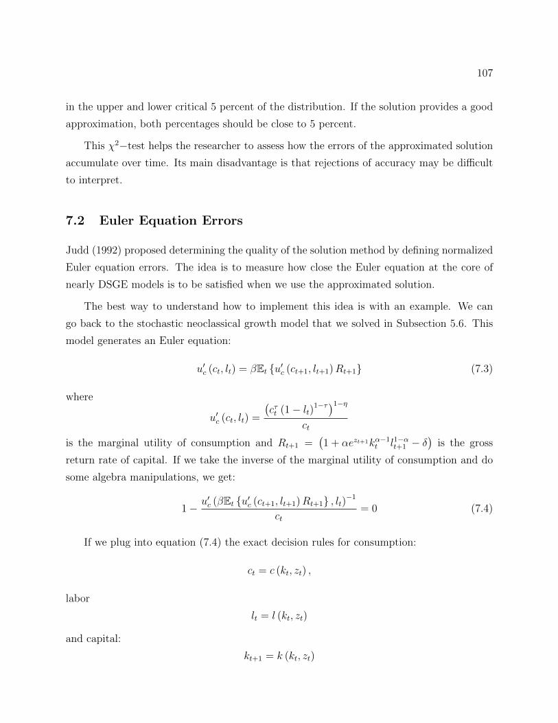
107

in the upper and lower critical 5 percent of the distribution. If the solution provides a good

approximation, both percentages should be close to 5 percent.

This χ2−test helps the researcher to assess how the errors of the approximated solution

accumulate over time. Its main disadvantage is that rejections of accuracy may be difficult

to interpret.

7.2 Euler Equation Errors

Judd (1992) proposed determining the quality of the solution method by defining normalized

Euler equation errors. The idea is to measure how close the Euler equation at the core of

nearly DSGE models is to be satisfied when we use the approximated solution.

The best way to understand how to implement this idea is with an example. We can

go back to the stochastic neoclassical growth model that we solved in Subsection 5.6. This

model generates an Euler equation:

u′c (ct, lt) = βEt u′c (ct+1, lt+1)Rt+1 (7.3)

where

u′c (ct, lt) =

(cτt (1− lt)1−τ)1−η

ct

is the marginal utility of consumption and Rt+1 =(1 + αezt+1kα−1

t l1−αt+1 − δ)

is the gross

return rate of capital. If we take the inverse of the marginal utility of consumption and do

some algebra manipulations, we get:

1− u′c (βEt u′c (ct+1, lt+1)Rt+1 , lt)−1

ct= 0 (7.4)

If we plug into equation (7.4) the exact decision rules for consumption:

ct = c (kt, zt) ,

labor

lt = l (kt, zt)

and capital:

kt+1 = k (kt, zt)

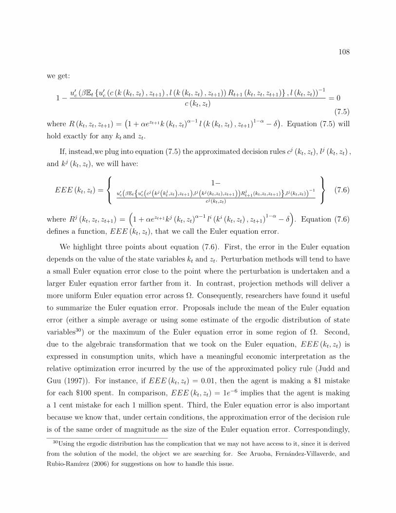
108

we get:

1− u′c (βEt u′c (c (k (kt, zt) , zt+1) , l (k (kt, zt) , zt+1))Rt+1 (kt, zt, zt+1) , l (kt, zt))−1

c (kt, zt)= 0

(7.5)

where R (kt, zt, zt+1) =(1 + αezt+1k (kt, zt)

α−1 l (k (kt, zt) , zt+1)1−α − δ). Equation (7.5) will

hold exactly for any kt and zt.

If, instead,we plug into equation (7.5) the approximated decision rules cj (kt, zt), lj (kt, zt) ,

and kj (kt, zt), we will have:

EEE (kt, zt) =

1−u′c(βEtu′c(cj(kj(kjt ,zt),zt+1),lj(kj(kt,zt),zt+1))Rjt+1(kt,zt,zt+1),lj(kt,zt))−1

cj(kt,zt)

(7.6)

where Rj (kt, zt, zt+1) =(

1 + αezt+1kj (kt, zt)α−1 li (ki (kt, zt) , zt+1)

1−α − δ)

. Equation (7.6)

defines a function, EEE (kt, zt), that we call the Euler equation error.

We highlight three points about equation (7.6). First, the error in the Euler equation

depends on the value of the state variables kt and zt. Perturbation methods will tend to have

a small Euler equation error close to the point where the perturbation is undertaken and a

larger Euler equation error farther from it. In contrast, projection methods will deliver a

more uniform Euler equation error across Ω. Consequently, researchers have found it useful

to summarize the Euler equation error. Proposals include the mean of the Euler equation

error (either a simple average or using some estimate of the ergodic distribution of state

variables30) or the maximum of the Euler equation error in some region of Ω. Second,

due to the algebraic transformation that we took on the Euler equation, EEE (kt, zt) is

expressed in consumption units, which have a meaningful economic interpretation as the

relative optimization error incurred by the use of the approximated policy rule (Judd and

Guu (1997)). For instance, if EEE (kt, zt) = 0.01, then the agent is making a $1 mistake

for each $100 spent. In comparison, EEE (kt, zt) = 1e−6 implies that the agent is making

a 1 cent mistake for each 1 million spent. Third, the Euler equation error is also important

because we know that, under certain conditions, the approximation error of the decision rule

is of the same order of magnitude as the size of the Euler equation error. Correspondingly,

30Using the ergodic distribution has the complication that we may not have access to it, since it is derived

from the solution of the model, the object we are searching for. See Aruoba, Fernandez-Villaverde, and

Rubio-Ramırez (2006) for suggestions on how to handle this issue.

109

Figure 13: log10 of Absolute Value of Euler Equation Error

the change in welfare is of the square order of the Euler equation error. Furthermore, the

constants involved in these error bounds can be related to model primitives (Santos (2000)).

Unfortunately, in some DSGE models it can be difficult to use algebraic transformations to

achieve an expression for the Euler equation error that is interpretable as consumption units

(or other natural economic unit).

Following the convention in the literature, we plot in Figure 13, the log10 |EEE (kt, zt)| of

the stochastic neoclassical growth model from Subsection 5.6. Taking the log10 eases reading:

a value of -3 means $1 mistake for each $1,000, a value of -4 a $1 mistake for each $10,000,

and so on. Figure 13 shows five lines, one for each value of productivity. As we hinted when

we described the Chebyshev-collocation projection method, this accuracy is outstanding.

To compare this performance of Chebyshev-collocation with other solution methods, we

reproduce, in Figures 14 and 15, results from Aruoba, Fernandez-Villaverde, and Rubio-

Ramırez (2006). That paper uses the same stochastic neoclassical growth model with only

a slightly different calibration (plus a few smaller details about how to handle zt). Both

figures display a transversal cut of the Euler equation errors when zt = 0 and for values of

capital between 70 and 130 percent of its steady-state value (23.14).

110

Figure 14: log10 of Absolute Value of Euler Equation Error

18 20 22 24 26 28 30

-9

-8

-7

-6

-5

-4

-3

Figure 8: Euler Equation Errors at z = 0, τ = 2 / σ = 0.007

Capital

Log1

0|E

uler

Equ

atio

n E

rror

|Perturbation 1: Log-Linear

Perturbation 1: Linear

Perturbation 2: Quadratic

Perturbation 5

In Figure 14, we plot the results for a first-order perturbation (in levels and in logs), a

second-order perturbation, and a fifth-order perturbation. First, perturbations have smaller

errors around the steady-state value of capital and deteriorate away from it. Second, there

is a considerable improvement when we go from a first- to a second-order approximation.

Third, a fifth-order approximation displays a great performance even 30 percent away from

the steady state.

In Figure 15, we plot the results from the first-order perturbation (as a comparison

with the previous graph), value function iteration (with a grid of one million points: 25,000

points for capital and 40 for the productivity level), finite elements (with 71 elements), and

Chebyshev polynomials (as in Subsection 5.6, still with 11 polynomials). The main lesson

from this graph is that the Euler equation errors are much flatter for projection methods

and value function iteration (another algorithm that delivers a global solution). The level

of each of the three functions is harder to interpret, since it depends on the number of grid

points (value function iteration), elements (finite elements), and Chebyshev polynomials.

Nevertheless, the performance of Chebyshev is again excellent and its run time much lower

than value function iteration and finite elements. This is not a surprise, since the decision

rules for the stochastic neoclassical growth model are sufficiently well-behaved for a spectral

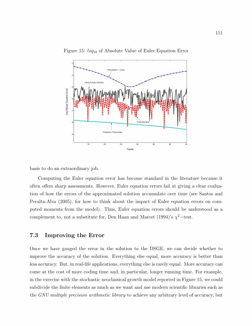
111

Figure 15: log10 of Absolute Value of Euler Equation Error

18 20 22 24 26 28 30

-9

-8

-7

-6

-5

-4

-3

Figure 9: Euler Equation Errors at z = 0, τ = 2 / σ = 0.007

Capital

Log1

0|E

uler

Equ

atio

n E

rror

|Perturbation 1: Linear

Value Function Iteration

Chebyshev Polynomials

Finite Elements

basis to do an extraordinary job.

Computing the Euler equation error has become standard in the literature because it

often offers sharp assessments. However, Euler equation errors fail at giving a clear evalua-

tion of how the errors of the approximated solution accumulate over time (see Santos and

Peralta-Alva (2005), for how to think about the impact of Euler equation errors on com-

puted moments from the model). Thus, Euler equation errors should be understood as a

complement to, not a substitute for, Den Haan and Marcet (1994)’s χ2−test.

7.3 Improving the Error

Once we have gauged the error in the solution to the DSGE, we can decide whether to

improve the accuracy of the solution. Everything else equal, more accuracy is better than

less accuracy. But, in real-life applications, everything else is rarely equal. More accuracy can

come at the cost of more coding time and, in particular, longer running time. For example,

in the exercise with the stochastic neoclassical growth model reported in Figure 15, we could

subdivide the finite elements as much as we want and use modern scientific libraries such as

the GNU multiple precision arithmetic library to achieve any arbitrary level of accuracy, but

112

at the cost of longer running times and more memory requirements. The researcher must

look at her needs and resources and, once inferior solution methods are rejected, select those

that best fit her goals.

But if the goal is indeed dependent on achieving additional accuracy, there are different

possibilities available. If a perturbation is being used, we can increase the order of the

perturbation. If a projection method is being used, we can increase the number of elements

in the basis. The researcher can also explore changes of variables to make the problem more

linear or switch the solution method.

Once the error of the model has been assessed, we are finally ready to move to Part II

and see how the DSGE model can account for the observed data.

113

Part II

Estimating DSGE Models

8 Confronting DSGE Models with Data

The preceding sections discussed how to compute an approximate solution for a DSGE model

conditional on its parameterization. Part II focuses on determining the DSGE model param-

eters based on the empirical evidence and assessing the model’s fit. More specifically, we ask

four fundamental questions: (i) How can one estimate the DSGE model parameters from

the observed macroeconomic time series? (ii) How well does the estimated DSGE model

capture salient features of the data? (iii) What are the quantitative implications of the es-

timated DSGE models with respect to, for instance, sources of business cycle fluctuations,

propagation of exogenous shocks, the effect of changes in macroeconomic policies, and the

future path of macroeconomic time series. (iv) How should one construct measures of uncer-

tainty for the parameters and the quantitative implications of the DSGE model? To answer

these questions, we begin by analytically solving a stylized New Keynesian DSGE model

in Section 8.1 and studying its properties in Section 8.2. DSGE model-implied population

moments, autocovariances, spectra, and impulse response functions have sample analogs in

the data, which are examined in Section 8.3. Macroeconomic time series exhibit trends that

may or may not be captured by the DSGE model, which is discussed in Section 8.4.

Part II of this chapter assumes that the reader has some basic familiarity with economet-

rics, at the level of a first-year PhD sequence in a U.S. graduate program. With the exception

of Canova (2007) and DeJong and Dave (2007) there are no textbooks that focus on the es-

timation of DSGE models. The literature has progressed quickly since these two books were

first written. The subsequent sections contain, in addition to a critical introduction to “stan-

dard methods,” an overview of the most recent developments in the literature, which include

identification conditions for DSGE models, identification-robust frequentist inference, and

sequential Monte Carlo techniques for Bayesian analysis. Unlike the recent monograph by

Herbst and Schorfheide (2015) which focuses on Bayesian computations, Part II of this chap-

ter also contains extensive discussions of the role of misspecification for econometric inference

and also covers frequentist methods.

114

8.1 A Stylized DSGE Model

Throughout Part II we consider a stylized New Keynesian DSGE model in its loglinearized

form.31 This model shares many of the features of its more realistic siblings that have been

estimated in the literature. It is a stripped-down version of the model developed in the work

by Christiano, Eichenbaum, and Evans (2005) and Smets and Wouters (2003). The specific

version presented below is taken from Del Negro and Schorfheide (2008) and obtained by

imposing several parameter restrictions. It is not suitable to be confronted with actual data,

but it can be solved analytically, which is useful for the subsequent exposition. For brevity,

we refer to this model as the stylized DSGE model in the remainder of this chapter.

The model economy consists of households, intermediate goods producers, final goods

producers, a monetary policy authority, and a fiscal authority. Macroeconomic fluctuations

are generated by four exogenous processes: a technology growth shock, zt, a shock that

generates shifts in the preference for leisure, φt, a price markup shock, λt, and a monetary

policy shock εR,t. We assume that the level of productivity Zt in the economy is evolving

exogenously according to a random walk with drift:

logZt = log γ + logZt−1 + zt, zt = ρzzt−1 + σzεz,t. (8.1)

The productivity process Zt induces a stochastic trend in output Xt and real wages Wt. To

facilitate the model solution, it is useful to detrend output and real wages by the level of

technology, defining xt = Xt/Zt and wt = Wt/Zt, respectively. In terms of the detrended

variables, the model has the following steady state:

x = x∗, w = lsh =1

1 + λ, π = π∗, R = π∗

γ

β. (8.2)

Here x∗ and π∗ are free parameters. The latter can be interpreted as the central bank’s target

inflation rate, whereas the former can in principle be derived from the weight on leisure in

the households’ utility function. The steady-state real wage w is equal to the steady-state

labor share lsh. The parameter λ can be interpreted as the steady-state markup charged

by the monopolistically competitive intermediate goods producers, β is the discount factor

of the households, and γ is the growth rate of technology. Under the assumption that the

production technology is linear in labor and labor is the only factor of production, the steady

state labor share equals the steady state of detrended wages. We also assume that all output

is consumed, which means that x can be interpreted as aggregate consumption.

31See Sections 4.1 and 4.5 for how to think about loglinearizations as a first-order perturbations.

115

8.1.1 Loglinearized Equilibrium Conditions

In terms of log-deviations from the steady state (denoted by ), i.e., x = log(xt/x), wt =

log(wt/w), πt = log(πt/π), and Rt = log(Rt/R), the equilibrium conditions of the model can

be stated as follows. The consumption Euler equation of the households takes the form

xt = Et+1[xt+1]−(Rt − E[πt+1]

)+ Et[zt+1]. (8.3)

The expected technology growth rate arises because the Euler equation is written in terms

of output in deviations from the stochastic trend induced by Zt. Assuming the absence of

nominal wage rigidities, the intratemporal Euler equation for the households leads to the

following labor supply equation:

wt = (1 + ν)xt + φt, (8.4)

where wt is the real wage, 1/(1 + ν) is the Frisch labor supply elasticity, xt is proportional

to hours worked, and φt is an exogenous labor supply shifter

φt = ρφφt−1 + σφεφ,t. (8.5)

We refer to φt as a preference shock.

The intermediate goods producers hire labor from the households and produce differ-

entiated products, indexed by j, using a linear technology of the form Xt(j) = ZtLt(j).

After detrending and loglinearization around steady-state aggregate output, the production

function becomes

xt(j) = Lt(j). (8.6)

Nominal price rigidity is introduced via the Calvo mechanism. In each period, firm j is unable

to re-optimize its nominal price with probability ζp. In this case, the firm simply adjusts its

price from the previous period by the steady-state inflation rate. With probability 1−ζp, the

firm can choose its price to maximize the expected sum of future profits. The intermediate

goods are purchased and converted into an aggregate good Xt by a collection of perfectly

competitive final goods producers using a constant-elasticity-of-substitution aggregator.

The optimality conditions for the two types of firms can be combined into the so-called

New Keynesian Phillips curve, which can be expressed as

πt = βEt[πt+1] + κp(wt + λt), κp =(1− ζpβ)(1− ζp)

ζp, (8.7)

116

where β is the households’ discount factor and λt can be interpreted as a price mark-up

shock, which exogenously evolves according to

λt = ρλλt−1 + σλελ,t. (8.8)

It is possibe to derive an aggregate resource constraint that relates the total amount of labor

Lt hired by the intermediate goods producers to the total aggregate output Xt produced

in the economy. Based on this aggregate resource constraint, it is possible to compute the

labor share of income, which, in terms of deviations from steady state is given by

lsht = wt. (8.9)

Finally, the central bank sets the nominal interest rate according to the feedback rule

Rt = ψπt + σRεR,t ψ = 1/β. (8.10)

We abstract from interest rate smoothing and the fact that central banks typically also

react to some measure of real activity, e.g., the gap between actual output and potential

output. The shock εR,t is an unanticipated deviation from the systematic part of the interest

rate feedback rule and is called a monetary policy shock. We assume that ψ = 1/β, which

ensures the existence of a unique stable solution to the system of linear rational expectations

difference equations and, as will become apparent below, simplifies the solution of the model

considerably. The fiscal authority determines the level of debt and lump-sum taxes such that

the government budget constraint is satisfied.

8.1.2 Model Solution

To solve the model, note that the economic state variables are φt, λt, zt, and εR,t. Due to

the fairly simply loglinear structure of the model, the aggregate laws of motion x(·), lsh(·),π(·), and R(·) are linear in the states and can be determined sequentially. We first eliminate

the nominal interest rate from the consumption Euler equation using (8.10):

xt = Et+1[xt+1]−(

1

βπt + σRεR,t − E[πt+1]

)+ Et[zt+1]. (8.11)

Now notice that the New Keynesian Phillips curve can be rewritten as

1

βπt − Et[πt+1] =

κpβ

((1 + ν)xt + φt + λt). (8.12)

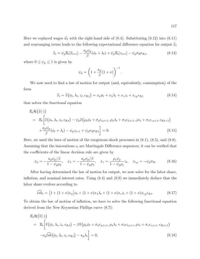
117

Here we replaced wages wt with the right-hand side of (8.4). Substituting (8.12) into (8.11)

and rearranging terms leads to the following expectational difference equation for output xt

xt = ψpEt[xt+1]− κpψpβ

(φt + λt) + ψpEt[zt+1]− ψpσRεR,t, (8.13)

where 0 ≤ ψp ≤ 1 is given by

ψp =

(1 +

κpβ

(1 + ν)

)−1

.

We now need to find a law of motion for output (and, equivalently, consumption) of the

form

xt = x(φt, λt, zt, εR,t

)= xφφt + xλλt + xzzt + xεRεR,t (8.14)

that solves the functional equation

EtH(x(·)

)= Et

[x(φt, λt, zt, εR,t

)− ψpx

(ρφφt + σφεφ,t+1, ρλλt + σλελ,t+1, ρzt + σzεz,t+1, εR,t+1

)+κpψpβ

(φt + λt)− ψpzt+1 + ψpσRεR,t

]= 0. (8.15)

Here, we used the laws of motion of the exogenous shock processes in (8.1), (8.5), and (8.8).

Assuming that the innovations εt are Martingale Difference sequences, it can be verified that

the coefficients of the linear decision rule are given by

xφ = − κpψp/β

1− ψpρφ, xλ = − κpψp/β

1− ψpρλ, xz =

ρzψp1− ψpρz

zt, xεR = −ψpσR. (8.16)

After having determined the law of motion for output, we now solve for the labor share,

inflation, and nominal interest rates. Using (8.4) and (8.9) we immediately deduce that the

labor share evolves according to

lsht =[1 + (1 + ν)xφ

]φt + (1 + ν)xλλt + (1 + ν)xzzt + (1 + ν)xεRεR,t. (8.17)

To obtain the law of motion of inflation, we have to solve the following functional equation

derived from the New Keynesian Phillips curve (8.7):

EtH(π(·)

)= Et

[π(φt, λt, zt, εR,t

)− βπ

(ρφφt + σφεφ,t+1, ρλλt + σλελ,t+1, ρzt + σzεz,t+1, εR,t+1

)−κplsh

(φt, λt, zt, εR,t

)− κpλt

]= 0, (8.18)

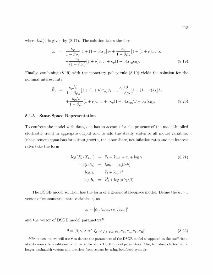
118

where lsh(·) is given by (8.17). The solution takes the form

πt =κp

1− βρφ[1 + (1 + ν)xφ

]φt +

κp1− βρλ

[1 + (1 + ν)xλ

]λt

+κp

(1− βρz)(1 + ν)xzzt + κp(1 + ν)xεRεR,t. (8.19)

Finally, combining (8.19) with the monetary policy rule (8.10) yields the solution for the

nominal interest rate

Rt =κp/β

1− βρφ[1 + (1 + ν)xφ

]φt +

κp/β

1− βρλ[1 + (1 + ν)xλ

]λt

+κp/β

1− βρz(1 + ν)xzzt +

[κp(1 + ν)xεR/β + σR

]εR,t. (8.20)

8.1.3 State-Space Representation

To confront the model with data, one has to account for the presence of the model-implied

stochastic trend in aggregate output and to add the steady states to all model variables.

Measurement equations for output growth, the labor share, net inflation rates and net interest

rates take the form

log(Xt/Xt−1) = xt − xt−1 + zt + log γ (8.21)

log(lsht) = lsht + log(lsh)

log πt = πt + log π∗

logRt = Rt + log(π∗γ/β).

The DSGE model solution has the form of a generic state-space model. Define the ns×1

vector of econometric state variables st as

st = [φt, λt, zt, εR,t, xt−1]′

and the vector of DSGE model parameters32

θ = [β, γ, λ, π∗, ζp, ν, ρφ, ρλ, ρz, σφ, σλ, σz, σR]′. (8.22)

32From now on, we will use θ to denote the parameters of the DSGE model as opposed to the coefficients

of a decision rule conditional on a particular set of DSGE model parameters. Also, to reduce clutter, we no

longer distinguish vectors and matrices from scalars by using boldfaced symbols.

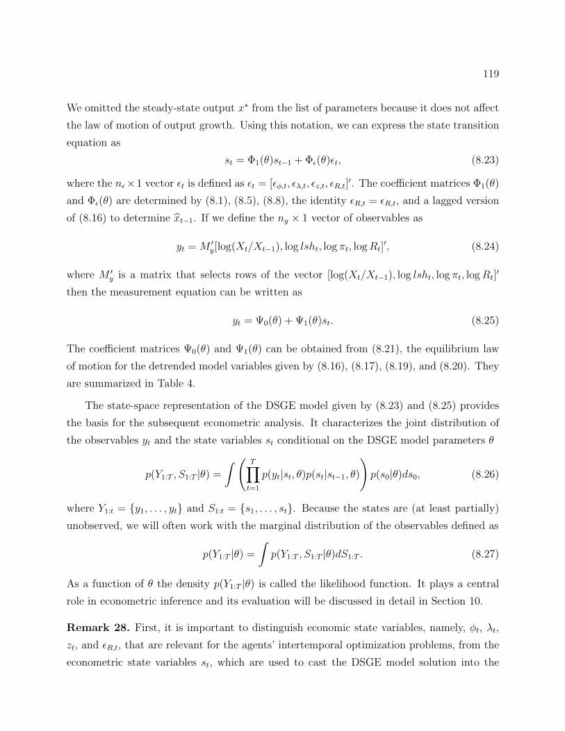
119

We omitted the steady-state output x∗ from the list of parameters because it does not affect

the law of motion of output growth. Using this notation, we can express the state transition

equation as

st = Φ1(θ)st−1 + Φε(θ)εt, (8.23)

where the nε×1 vector εt is defined as εt = [εφ,t, ελ,t, εz,t, εR,t]′. The coefficient matrices Φ1(θ)

and Φε(θ) are determined by (8.1), (8.5), (8.8), the identity εR,t = εR,t, and a lagged version

of (8.16) to determine xt−1. If we define the ny × 1 vector of observables as

yt = M ′y[log(Xt/Xt−1), log lsht, log πt, logRt]

′, (8.24)

where M ′y is a matrix that selects rows of the vector [log(Xt/Xt−1), log lsht, log πt, logRt]

′

then the measurement equation can be written as

yt = Ψ0(θ) + Ψ1(θ)st. (8.25)

The coefficient matrices Ψ0(θ) and Ψ1(θ) can be obtained from (8.21), the equilibrium law

of motion for the detrended model variables given by (8.16), (8.17), (8.19), and (8.20). They

are summarized in Table 4.

The state-space representation of the DSGE model given by (8.23) and (8.25) provides

the basis for the subsequent econometric analysis. It characterizes the joint distribution of

the observables yt and the state variables st conditional on the DSGE model parameters θ

p(Y1:T , S1:T |θ) =

∫ ( T∏t=1

p(yt|st, θ)p(st|st−1, θ)

)p(s0|θ)ds0, (8.26)

where Y1:t = y1, . . . , yt and S1:t = s1, . . . , st. Because the states are (at least partially)

unobserved, we will often work with the marginal distribution of the observables defined as

p(Y1:T |θ) =

∫p(Y1:T , S1:T |θ)dS1:T . (8.27)

As a function of θ the density p(Y1:T |θ) is called the likelihood function. It plays a central

role in econometric inference and its evaluation will be discussed in detail in Section 10.

Remark 28. First, it is important to distinguish economic state variables, namely, φt, λt,

zt, and εR,t, that are relevant for the agents’ intertemporal optimization problems, from the

econometric state variables st, which are used to cast the DSGE model solution into the

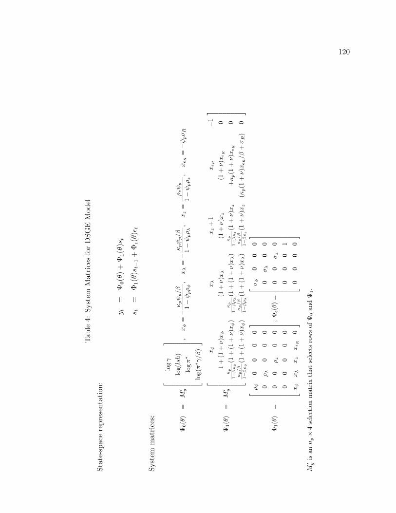
120

Tab

le4:

Syst

emM

atri

ces

for

DSG

EM

odel

Sta

te-s

pac

ere

pre

senta

tion

:

y t=

Ψ0(θ

)+

Ψ1(θ

)st

s t=

Φ1(θ

)st−

1+

Φε(θ)ε t

Syst

emm

atri

ces:

Ψ0(θ

)=

M′ y

lo

gγ

log(lsh

)

logπ∗

log(π∗ γ/β

)

,xφ

=−κpψp/β

1−ψpρφ,

xλ

=−κpψp/β

1−ψpρλ,

xz

=ρzψp

1−ψpρz,

xε R

=−ψpσR

Ψ1(θ

)=

M′ y

xφ

xλ

xz

+1

xε R

−1

1+

(1+ν

)xφ

(1+ν

)xλ

(1+ν

)xz

(1+ν

)xε R

0κp

1−βρφ

(1+

(1+ν

)xφ)

κp

1−βρλ

(1+

(1+ν

)xλ)

κp

1−βρz(1

+ν

)xz

+κp(1

+ν

)xε R

0κp/β

1−βρφ

(1+

(1+ν

)xφ)

κp/β

1−βρλ

(1+

(1+ν

)xλ)

κp/β

1−βρz(1

+ν

)xz

(κp(1

+ν

)xε R/β

+σR

)0

Φ1(θ

)=

ρφ

00

00

0ρλ

00

0

00

ρz

00

00

00

0

xφ

xλ

xz

xε R

0

,Φε(θ

)=

σφ

00

0

0σλ

00

00

σz

0

00

01

00

00

M′ y

isan

ny×

4se

lect

ion

mat

rix

that

sele

cts

row

sof

Ψ0

an

dΨ

1.

121

state-space form given by (8.23) and (8.25). The economic state variables of our simple

model are all exogenous. As we have seen in Section 4.3, the vector of state variables of

a richer DSGE model also may include one or more endogenous variables, e.g., the capital

stock. Second, output growth in the measurement equation could be replaced by the level

of output. This would require adding x∗ to the parameter vector θ, eliminating xt−1 from

st, adding logZt/γt to st, and accounting for the deterministic trend component (log γ)t in

log output in the measurement equation. Third, the measurement equation (8.25) could be

augmented by measurement errors. Fourth, if a DSGE model is solved with a higher-order

perturbation or projection method, then, depending on how exactly the state vector st is

defined, the state-transition equation (8.23), the measurement equation (8.25), or both are

non-linear.

8.2 Model Implications

Once we specify a distribution for the innovation vector εt the probability distribution of the

DSGE model variables is fully determined. Recall that the innovation standard deviations

were absorbed into the definition of the matrix Φε(θ) in (8.25). For the sake of concreteness,

we assume that

εt ∼ iidN(0, I), (8.28)

where I denotes the identity matrix. Based on the probabilistic structure of the DSGE

model, we can derive a number of implications from the DSGE model that will later be used

to construct estimators of the parameter vector θ and evaluate the fit of the model. For now,

we fix θ to the values listed in Table 5.

8.2.1 Autocovariances and Forecast Error Variances

DSGE models are widely used for business cycle analysis. In this regard, the model-implied

variances, autocorrelations, and cross-correlations are important objects. For linear DSGE

models it is straightforward to compute the autocovariance function from the state-space

representation given by (8.23) and (8.25).33 Using the notation

Γyy(h) = E[ytyt−h], Γss(h) = E[stst−h], and Γys(h) = E[yts′t−h]

33For the parameters in Table 5, the largest (in absolute value) eigenvalue of the matrix Φ1(θ) in (8.23) is

less than one, which implies that the VAR(1) law of motion for st is covariance stationary.

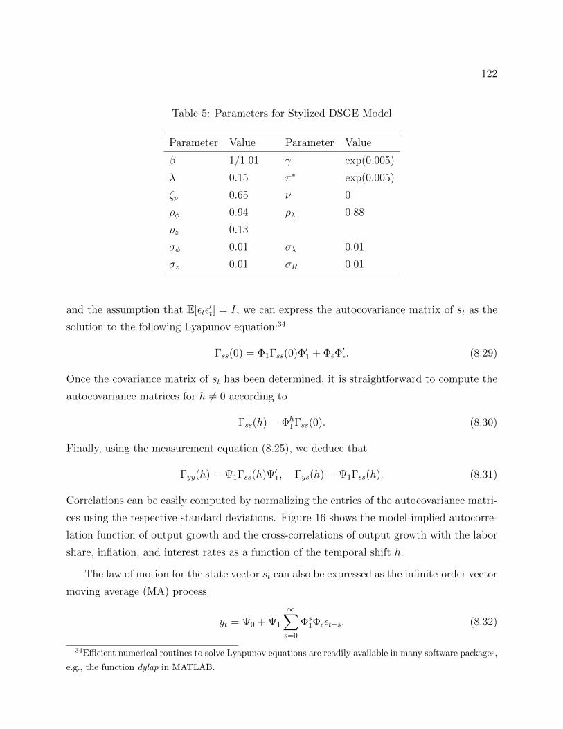
122

Table 5: Parameters for Stylized DSGE Model

Parameter Value Parameter Value

β 1/1.01 γ exp(0.005)

λ 0.15 π∗ exp(0.005)

ζp 0.65 ν 0

ρφ 0.94 ρλ 0.88

ρz 0.13

σφ 0.01 σλ 0.01

σz 0.01 σR 0.01

and the assumption that E[εtε′t] = I, we can express the autocovariance matrix of st as the

solution to the following Lyapunov equation:34

Γss(0) = Φ1Γss(0)Φ′1 + ΦεΦ′ε. (8.29)

Once the covariance matrix of st has been determined, it is straightforward to compute the

autocovariance matrices for h 6= 0 according to

Γss(h) = Φh1Γss(0). (8.30)

Finally, using the measurement equation (8.25), we deduce that

Γyy(h) = Ψ1Γss(h)Ψ′1, Γys(h) = Ψ1Γss(h). (8.31)

Correlations can be easily computed by normalizing the entries of the autocovariance matri-

ces using the respective standard deviations. Figure 16 shows the model-implied autocorre-

lation function of output growth and the cross-correlations of output growth with the labor

share, inflation, and interest rates as a function of the temporal shift h.

The law of motion for the state vector st can also be expressed as the infinite-order vector

moving average (MA) process

yt = Ψ0 + Ψ1

∞∑s=0

Φs1Φεεt−s. (8.32)

34Efficient numerical routines to solve Lyapunov equations are readily available in many software packages,

e.g., the function dylap in MATLAB.

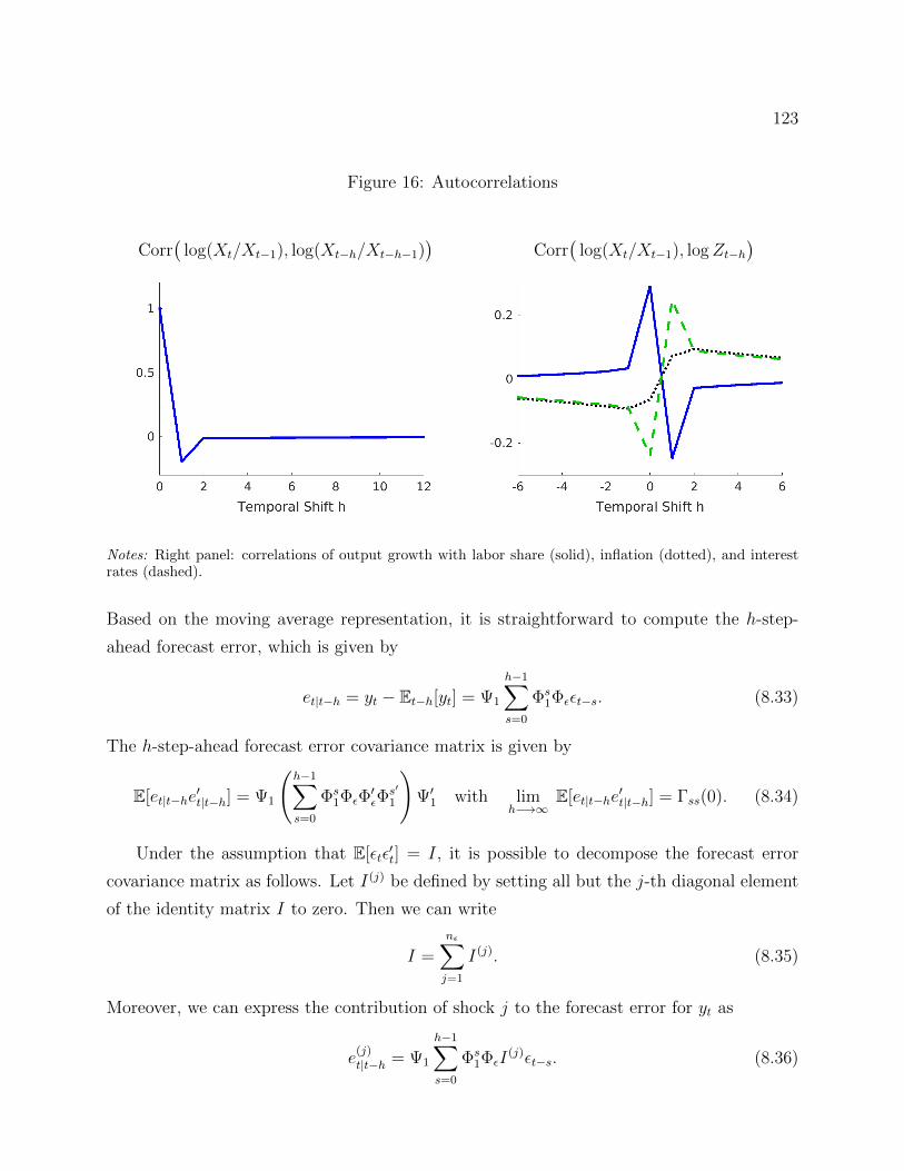
123

Figure 16: Autocorrelations

Corr(

log(Xt/Xt−1), log(Xt−h/Xt−h−1))

Corr(

log(Xt/Xt−1), logZt−h)

Notes: Right panel: correlations of output growth with labor share (solid), inflation (dotted), and interestrates (dashed).

Based on the moving average representation, it is straightforward to compute the h-step-

ahead forecast error, which is given by

et|t−h = yt − Et−h[yt] = Ψ1

h−1∑s=0

Φs1Φεεt−s. (8.33)

The h-step-ahead forecast error covariance matrix is given by

E[et|t−he′t|t−h] = Ψ1

(h−1∑s=0

Φs1ΦεΦ

′εΦ

s′

1

)Ψ′1 with lim

h−→∞E[et|t−he

′t|t−h] = Γss(0). (8.34)

Under the assumption that E[εtε′t] = I, it is possible to decompose the forecast error

covariance matrix as follows. Let I(j) be defined by setting all but the j-th diagonal element

of the identity matrix I to zero. Then we can write

I =nε∑j=1

I(j). (8.35)

Moreover, we can express the contribution of shock j to the forecast error for yt as

e(j)t|t−h = Ψ1

h−1∑s=0

Φs1ΦεI

(j)εt−s. (8.36)

124

Thus, the contribution of shock j to the forecast error variance of observation yi,t is given

by the ratio

FEVD(i, j, h) =

[Ψ1

(∑h−1s=0 Φs

1ΦεI(j)Φ′εΦ

s′1

)Ψ′1

]ii[

Ψ1

(∑h−1s=0 Φs

1ΦεΦ′εΦs′1

)Ψ′1

]ii

, (8.37)

where [A]ij denotes element (i, j) of a matrix A. Figure 17 shows the contribution of the

four shocks to the forecast error variance of output growth, the labor share, inflation, and

interest rates in the stylized DSGE model. Given the choice of parameters θ in Table 5, most

of the variation in output growth is due to the technology and the monetary policy shocks.

The labor share fluctuations are dominated by the mark-up shock λt, in particular in the

long run. Inflation and interest rate movements are strongly influenced by the preference

shock φt and the mark-up shock λt.

8.2.2 Spectrum

Instead of studying DSGE model implications over different forecasting horizons, one can also

consider different frequency bands. There is a long tradition of frequency domain analysis

in the time series literature. A classic reference is Priestley (1981). We start with a brief

discussion of the linear cyclical model, which will be useful for interpreting some of the

formulas presented subsequently. Suppose that yt is a scalar time series that follows the

process

yt = 2m∑j=1

aj(

cos θj cos(ωjt)− sin θj sin(ωjt)), (8.38)

where θj ∼ iidU [−π, π] and 0 ≤ ωj ≤ ωj+1 ≤ π. The random variables θj cause a phase shift

of the cycle and are assumed to be determined in the infinite past. In a nutshell, the model

in (8.38) expresses the variable yt as the sum of sine and cosine waves that differ in their

frequency. The interpretation of the ωj’s depends on the length of the period t. Suppose the

model is designed for quarterly data and ωj = (2π)/32. This means that it takes 32 periods

to complete the cycle. Business cycles typically comprise cycles that have a duration of 8 to

32 quarters, which would correspond to ωj ∈ [0.196, 0.785] for quarterly t.

Using Euler’s formula, we rewrite the cyclical model in terms of an exponential function:

yt =m∑

j=−m

A(ωj)eiωjt, (8.39)

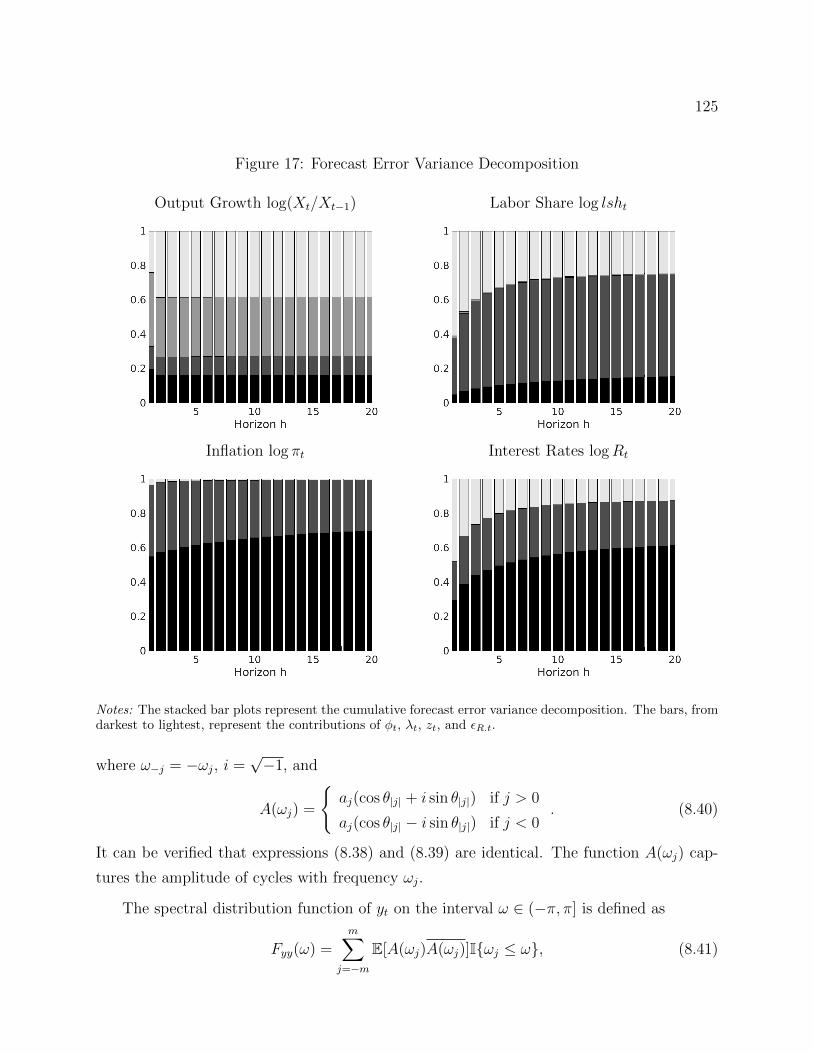
125

Figure 17: Forecast Error Variance Decomposition

Output Growth log(Xt/Xt−1) Labor Share log lsht

Inflation log πt Interest Rates logRt

Notes: The stacked bar plots represent the cumulative forecast error variance decomposition. The bars, fromdarkest to lightest, represent the contributions of φt, λt, zt, and εR.t.

where ω−j = −ωj, i =√−1, and

A(ωj) =

aj(cos θ|j| + i sin θ|j|) if j > 0

aj(cos θ|j| − i sin θ|j|) if j < 0. (8.40)

It can be verified that expressions (8.38) and (8.39) are identical. The function A(ωj) cap-

tures the amplitude of cycles with frequency ωj.

The spectral distribution function of yt on the interval ω ∈ (−π, π] is defined as

Fyy(ω) =m∑

j=−m

E[A(ωj)A(ωj)]Iωj ≤ ω, (8.41)

126

where Iωj ≤ ω denotes the indicator function that is one if ωj ≤ ω and z = x− iy is the

complex conjugate of z = x + iy. If Fyy(ω) is differentiable with respect to ω, then we can

define the spectral density function as

fyy(ω) = dFyy(ω)dω. (8.42)

If a process has a spectral density function fyy(ω), then the covariances can be expressed as

Γyy(h) =

∫(−π,π]

eihωfyy(ω)dω. (8.43)

For the linear cyclical model in (8.38) the autovariances are given by

Γyy(h) =m∑

j=−m

E[A(ωj)A(ωj)]eiωjh =

m∑j=−m

a2jeiωjh. (8.44)

The spectral density uniquely determines the entire sequence of autocovariances. Moreover,

the converse is also true. The spectral density can be obtained from the autocovariances of

yt as follows:

fyy(ω) =1

2π

∞∑h=−∞

Γyy(h)e−iωh. (8.45)

The formulas (8.43) and (8.45) imply that the spectral density function and the sequence

of autocovariances contain the same information. Their validity is not restricted to the linear

cyclical model and they extend to vector-valued yt’s. Recall that for the DSGE model defined

by the state-space system (8.23) and (8.25) the autocovariance function for the state vector

st was defined as Γss(h) = Φh1Γss(0). Thus,

fss(ω) =1

2π

∞∑h=−∞

Φh1Γss(0)e−iωh (8.46)

=1

2π

(I − Φ′1e

iω)−1

ΦεΦ′ε

(I − Φ1e

−iω)−1.

The contribution of shock j to the spectral density is given by

f (j)ss (ω) =

1

2π

(I − Φ′1e

iω)−1

ΦεI(j)Φ′ε(I − Φ1e

−iω)−1. (8.47)

The spectral density for the observables yt (and the contribution of shock j to the spectral

density) can be easily obtained as

fyy(ω) = Ψ1fss(ω)Ψ′1 and f (j)yy (ω) = Ψ1f

(j)ss (ω)Ψ′1. (8.48)

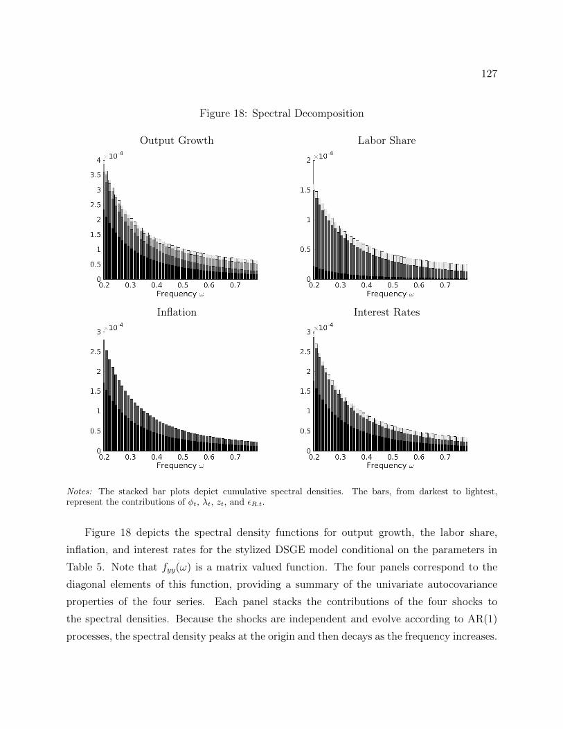
127

Figure 18: Spectral Decomposition

Output Growth Labor Share

Inflation Interest Rates

Notes: The stacked bar plots depict cumulative spectral densities. The bars, from darkest to lightest,represent the contributions of φt, λt, zt, and εR.t.

Figure 18 depicts the spectral density functions for output growth, the labor share,

inflation, and interest rates for the stylized DSGE model conditional on the parameters in

Table 5. Note that fyy(ω) is a matrix valued function. The four panels correspond to the

diagonal elements of this function, providing a summary of the univariate autocovariance

properties of the four series. Each panel stacks the contributions of the four shocks to

the spectral densities. Because the shocks are independent and evolve according to AR(1)

processes, the spectral density peaks at the origin and then decays as the frequency increases.

128

8.2.3 Impulse Response Functions

An important tool for studying the dynamic effects of exogenous shocks are impulse response

functions (IRFs). Formally, impulse responses in a DSGE model can be defined as the

difference between two conditional expectations:

IRF(i, j, h|st−1) = E[yi,t+h

∣∣ st−1, εj,t = 1]− E

[yi,t+h

∣∣ st−1

]. (8.49)

Both expectations are conditional on the initial state st−1 and integrate over current and

future realizations of the shocks εt. However, the first term also conditions on εj,t = 1,

whereas the second term averages of εj,t. In a linearized DSGE model with a state-space

representation of the form (8.23) and (8.25), we can use the linearity and the property that

E[εt+h|st−1] = 0 for h = 0, 1, . . . to deduce that

IRF(., j, h) = Ψ1∂

∂εj,tst+h = Ψ1Φh

1 [Φε].j, (8.50)

where [A].j is the j-th column of a matrix A. We dropped st−1 from the conditioning set to

simplify the notation.

Figure 19 depicts the impulse response functions for the stylized DSGE model of log

output to the four structural shocks, which can be easily obtained from (8.16) and the

laws of motion of the exogenous shock processes. The preference and mark-up shocks lower

output upon impact. Subsequently, output reverts back to its steady state. The speed of the

reversion is determined by the autoregressive coefficient associated with the exogenous shock

process. The technology growth shock raises the log level of output permanently, whereas a

monetary policy shock has only a one-period effect on output.

8.2.4 Conditional Moment Restrictions

The intertemporal optimality conditions take the form of conditional moment restrictions.

For instance, re-arranging the terms in the New Keynesian Phillips (8.7) curve, we can write

Et−1

[πt−1 − βπt − κp(lsht−1 + λt−1)

]= 0. (8.51)

The conditional moment condition can be converted into a vector of unconditional moment

conditions as follows. Let Ft denote the sigma algebra generated by the infinite histories of

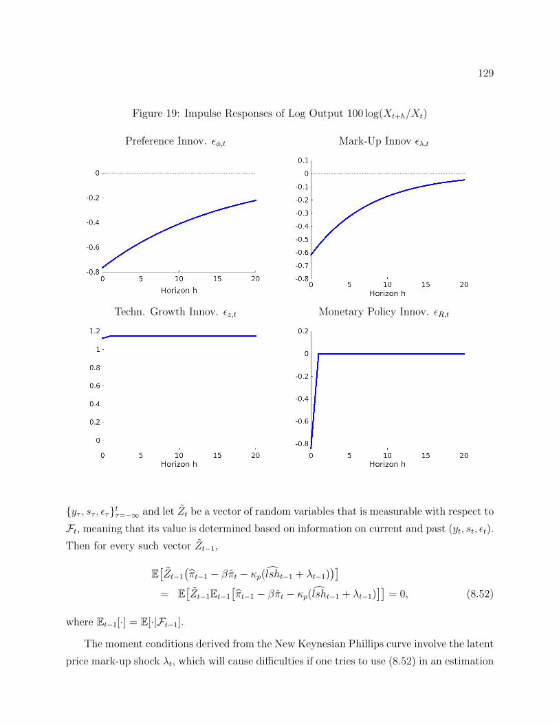
129

Figure 19: Impulse Responses of Log Output 100 log(Xt+h/Xt)

Preference Innov. εφ,t Mark-Up Innov ελ,t

Techn. Growth Innov. εz,t Monetary Policy Innov. εR,t

yτ , sτ , ετtτ=−∞ and let Zt be a vector of random variables that is measurable with respect to

Ft, meaning that its value is determined based on information on current and past (yt, st, εt).

Then for every such vector Zt−1,

E[Zt−1

(πt−1 − βπt − κp(lsht−1 + λt−1)

)]= E

[Zt−1Et−1

[πt−1 − βπt − κp(lsht−1 + λt−1)

]]= 0, (8.52)

where Et−1[·] = E[·|Ft−1].

The moment conditions derived from the New Keynesian Phillips curve involve the latent

price mark-up shock λt, which will cause difficulties if one tries to use (8.52) in an estimation

130

objective function. Now consider the consumption Euler equation (8.3) instead. Recall that

the measurement equations imply that

xt − xt−1 + zt = logXt − logXt−1 − log γ and Rt = logRt − log(π∗γ/β).

Thus, we can write

Et−1

[− log(Xt/Xt−1) + logRt−1 − log πt − log(1/β)

]= 0. (8.53)

The terms γ and log π∗ that appear in the steady-state formulas for the nominal interest rate

and inflation cancel and the conditional moment condition only depends on observables and

the model parameters, but not on latent variables. Finally, as long as the monetary policy

shock satisfies the martingale difference sequences property Et−1[εR,t] = 0, we obtain from

the monetary policy rule the condition that

Et−1

[logRt − log(γ/β)− ψ log πt − (1− ψ) log π∗] = 0. (8.54)

Both (8.53) and (8.54) can be converted into an unconditional moment condition using an

Ft−1 measurable random vector Zt−1 as in (8.52).

8.2.5 Analytical Calculation of Moments Versus Simulation Approximations

As previously shown, formulas for autocovariance functions, spectra, and impulse response

functions for a linearized DSGE model can be derived analytically from the state-space

representation. These analytical expressions can then be numerically evaluated for different

vectors of parameter values θ. For DSGE models solved with perturbation methods, there

are also analytical formulas available that exploit a conditionally linear structure of some

perturbation solutions; see Andreasen, Fernandez-Villaverde, and Rubio-Ramırez (2013).

For a general nonlinear DSGE model, the implied moments have to be computed using

Monte Carlo simulation. For instance, let Y ∗1:T denote a sequence of observations simulated

from the state-space representation of the DSGE model by drawing an initial state vector s0

and innovations εt from their model-implied distributions, then

1

T

T∑t=1

y∗ta.s.−→ E[yt], (8.55)

131

provided that the DSGE model-implied yt is strictly stationary and ergodic.35 The downside

of Monte Carlo approximations is that they are associated with a simulation error. We

will come back to this problem in Section 11.2, when we use simulation approximations of

moments to construct estimators of θ.

8.3 Empirical Analogs

We now examine sample analogs of the population moments derived from the state-space

representation of the DSGE model using U.S. data. The time series were downloaded from

the FRED database maintained by the Federal Reserve Bank of St. Louis and we report

the series labels in parentheses. For real aggregate output, we use quarterly, seasonally

adjusted GDP at the annual rate that has been pegged to 2009 dollars (GDPC96). We turn

GDP into growth rates by taking logs and then differencing. The labor share is defined

as Compensation of Employees (COE) divided by nominal GDP (GDP). Both series are

quarterly and seasonally adjusted at the annual rate. We use the log labor share as the

observable. Inflation rates are computed from the implicit price deflator (GDPDEF) by

taking log differences. Lastly, for the interest rate, we use the Effective Federal Funds Rate

(FEDFUNDS), which is monthly, and not seasonally adjusted. Quarterly interest rates are

obtained by taking averages of the monthly rates. Throughout this section we focus on

the post-Great Moderation and pre-Great Recession period and restrict our sample from

1984:Q1 to 2007:Q4.

8.3.1 Autocovariances

The sample analog of the population autocovariance Γyy(h) is defined as

Γyy(h) =1

T

T∑t=h

(yt − µy)(yt−h − µy)′, where µy =1

T

T∑t=1

yt. (8.56)

Under suitable regularity conditions, e.g., covariance stationarity of the vector process yt,

a sufficiently fast decay of the serial correlation in yt, and some bounds on higher-order

35A sequence of random variables XT converges to a limit random variable X almost surely (a.s.) if the

set of trajectories for which XT 6−→ X has probability zero.

132

moments of yt, the sample autocovariance Γyy(h) converges to the population autocovariance

Γyy(h), satisfying a strong law of large numbers (SLLN) and a central limit theorem (CLT).

If the object of interest is a sequence of autocovariance matrices, then it might be more

efficient to first estimate an auxiliary model and then convert the parameter estimates of

the auxiliary model into estimates of the autocovariance sequence. A natural class of aux-

iliary models is provided by linear vector autoregressions (VARs). For illustrative purposes

consider the following VAR(1):

yt = Φ1yt−1 + Φ0 + ut, ut ∼ iid(0,Σ). (8.57)

The OLS estimator of Φ1 can be approximated by

Φ1 = Γyy(1)Γ−1yy (0) +Op(T

−1), Σ = Γyy(0)− Γyy(1)Γ−1yy (0)Γ′yy(1) +Op(T

−1) (8.58)

The Op(T−1) terms arise because the range of the summations in the definition of the sample

autocovariances in (8.56) and the definition of the OLS estimator are not exactly the same.36

Suppose that now we plug the OLS estimator into the autocovariance formulas associated

with the VAR(1) (see (8.29) and (8.30)), then:

ΓVyy(0) = Γyy(0) +Op(T−1), ΓVyy(h) =

(Γyy(1)Γ−1

yy (0))h

Γyy(0) +Op(T−1). (8.59)

Note that for h = 0, 1 we obtain ΓVyy(1) = Γyy(1) + Op(T−1). For h > 1 the VAR(1) plug-in

estimate of the autocovariance matrix differs from the sample autocovariance matrix. If

the actual time series are well approximated by a VAR(1), then the plug-in autocovariance

estimate tends to be more efficient than the sample autocovariance estimate Γyy(h); see, for

instance, Schorfheide (2005b).

In practice, a VAR(1) may be insufficient to capture the dynamics of a time series yt. In

this case the autocovariances can be obtained from a VAR(p)

yt = Φ1yt−1 + . . .+ Φpyt−p + Φ0 + ut, ut ∼ iid(0,Σ). (8.60)

The appropriate lag length p can be determined with a model selection criterion, e.g., the

Schwarz (1978) criterion, which is often called the Bayesian information criterion (BIC).

The notationally easiest way (but not the computationally fastest way) is to rewrite the

36We say that a sequence of random variables is Op(T−1) if TXT is stochastically bounded as T −→∞.

133

VAR(p) in companion form. This entails expressing the law of motion for the stacked vector

yt = [y′t, y′t−1, . . . , y

′t−p+1] as VAR(1):

yt = Φ1yt−1 + Φ0 + ut, ut ∼ iid(0, Σ), (8.61)

where

Φ1 =

Φ1 . . . Φp−1 Φp

In×n . . . 0n×n 0n×n...

. . ....

...

0n×n . . . In×n 0n×n

, Φ0 =

[Φ0

0n(p−1)×1

],

εt =

[εt

0n(p−1)×1

], Σ =

[Σ 0n×n(p−1)

0n(p−1)×n 0n(p−1)×n(p−1)

].

The autocovariances for yt are then obtained by adjusting the VAR(1) formulas (8.59) to yt

and reading off the desired submatrices that correspond to the autocovariance matrices for

yt using the selection matrix M ′ = [In, 0n×n(p−1)] such that yt = M ′yt.

We estimate a VAR for output growth, labor share, inflation, and interest rates. The

lag length p = 1 is determined by the BIC. The left panel of Figure 20 shows sample cross-

correlations (obtained from Γyy(h) in (8.56)) between output growth and leads and lags of

the labor share, inflation, and interest rates, respectively. The right panel depicts correlation

functions derived from the estimated VAR(1). The two sets of correlation functions are qual-

itatively similar but quantitatively different. Because the VAR model is more parsimonious,

the VAR-implied correlation functions are smoother.

8.3.2 Spectrum

An intuitively plausible estimate of the spectrum is the sample periodogram, defined as

fyy(ω) =1

2π

T−1∑h=−T+1

Γyy(h)e−iωh =1

2π

(Γyy(0) +

T−1∑h=1

(Γyy(h) + Γyy(h)′) cosωh

). (8.62)

While the sample periodogram is an asymptotically unbiased estimator of the population

spectral density, it is inconsistent because its variance does not vanish as the sample size

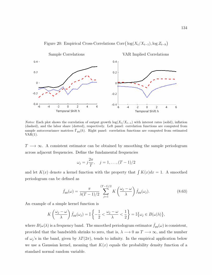
134

Figure 20: Empirical Cross-Correlations Corr(

log(Xt/Xt−1), logZt−h)

Sample Correlations VAR Implied Correlations

Notes: Each plot shows the correlation of output growth log(Xt/Xt−1) with interest rates (solid), inflation(dashed), and the labor share (dotted), respectively. Left panel: correlation functions are computed from

sample autocovariance matrices Γyy(h). Right panel: correlation functions are computed from estimatedVAR(1).

T −→ ∞. A consistent estimator can be obtained by smoothing the sample periodogram

across adjacent frequencies. Define the fundamental frequencies

ωj = j2π

T, j = 1, . . . , (T − 1)/2

and let K(x) denote a kernel function with the property that∫K(x)dx = 1. A smoothed

periodogram can be defined as

fyy(ω) =π

λ(T − 1)/2

(T−1)/2∑j=1

K

(ωj − ωλ

)fyy(ωj). (8.63)

An example of a simple kernel function is

K

(ωj − ωλ

)fyy(ωj) = I

−1

2<ωj − ωλ

<1

2

= Iωj ∈ B(ω|λ)

,

where B(ω|λ) is a frequency band. The smoothed periodogram estimator fyy(ω) is consistent,

provided that the bandwidth shrinks to zero, that is, λ −→ 0 as T −→ ∞, and the number

of ωj’s in the band, given by λT (2π), tends to infinity. In the empirical application below

we use a Gaussian kernel, meaning that K(x) equals the probability density function of a

standard normal random variable.

135

An estimate of the spectral density can also be obtained indirectly through the estimation

of the VAR(p) in (8.60). Define

Φ = [Φ1, . . . ,Φp,Φ0]′ and M(z) = [Iz, . . . , Izp],

and let Φ be an estimator of Φ. Then a VAR(p) plug-in estimator of the spectral density is

given by

fVyy(ω) =1

2π[I − Φ′M ′(e−iω)]−1Σ[I −M(e−iω)Φ]−1. (8.64)

This formula generalizes the VAR(1) spectral density in (8.46) to a spectral density for a

VAR(p).

Estimates of the spectral densities of output growth, log labor share, inflation, and

interest rates are reported in Figure 21. The shaded areas highlight the business cycle

frequencies. Because the autocorrelation of output growth is close to zero, the spectral

density is fairly flat. The other three series have more spectral mass at the low frequency,

which is a reflection of the higher persistence. The labor share has a pronounced hump-

shaped spectral density, whereas the other spectral densities of interest and inflation rates are

monotonically decreasing in the frequency ω. The smoothness of the periodogram estimates

fyy(ω) depends on the choice of the bandwidth. The figure is based on a Gaussian kernel with

standard deviation 0.15, which, roughly speaking, averages the sample periodogram over a

frequency band of 0.6. While the shapes of the smoothed periodograms and the VAR-based

spectral estimates are qualitatively similar, the spectral density is lower according to the

estimated VAR.

8.3.3 Impulse Response Functions

The VAR(p) in (8.60) is a so-called reduced-form VAR because the innovations ut do not

have a specific structural interpretation – they are simply one-step-ahead forecast errors.

The impulse responses that we constructed for the DSGE model are responses to innova-

tions in the structural shock innovations that contribute to the forecast error for several

observables simultaneously. In order to connect VAR-based impulse responses to DSGE

model-based responses, one has to link the one-step-ahead forecast errors to a vector of

structural innovations εt. We assume that

ut = Φεεt = ΣtrΩεt, (8.65)

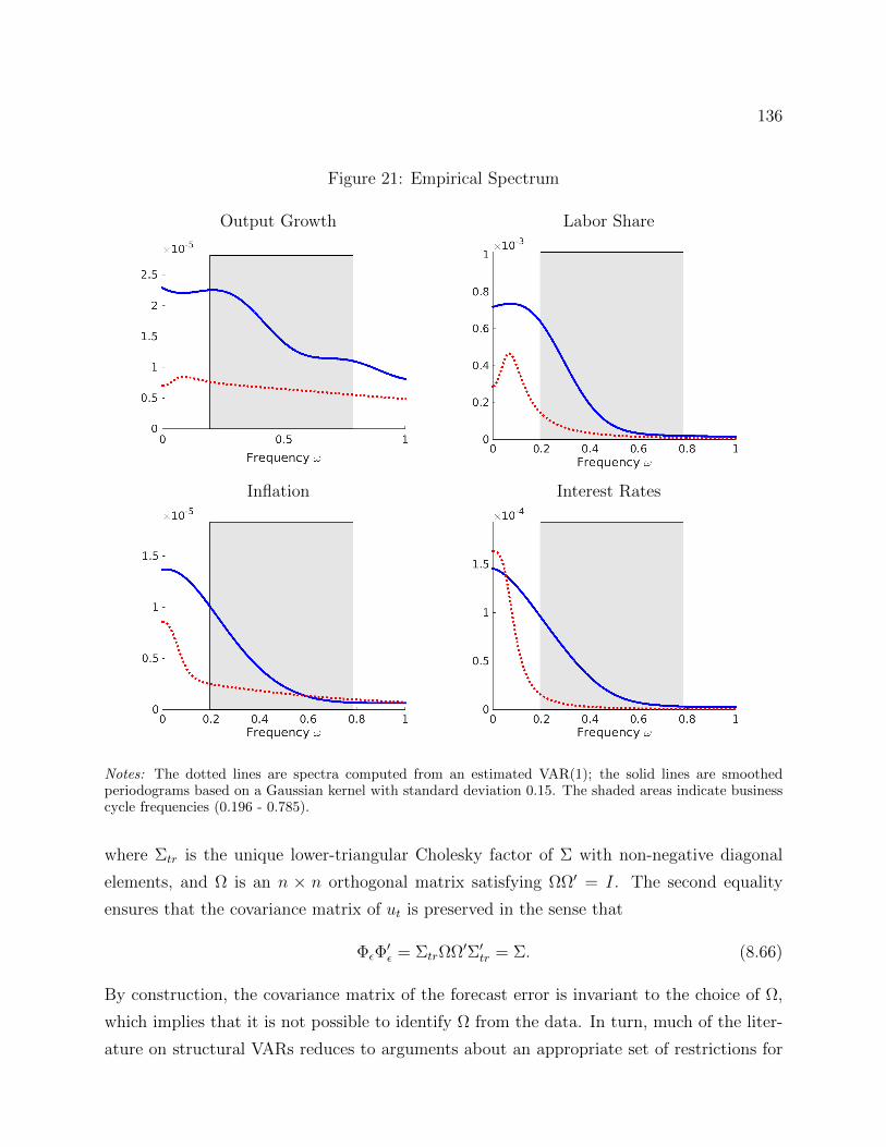
136

Figure 21: Empirical Spectrum

Output Growth Labor Share

Inflation Interest Rates

Notes: The dotted lines are spectra computed from an estimated VAR(1); the solid lines are smoothedperiodograms based on a Gaussian kernel with standard deviation 0.15. The shaded areas indicate businesscycle frequencies (0.196 - 0.785).

where Σtr is the unique lower-triangular Cholesky factor of Σ with non-negative diagonal

elements, and Ω is an n × n orthogonal matrix satisfying ΩΩ′ = I. The second equality

ensures that the covariance matrix of ut is preserved in the sense that

ΦεΦ′ε = ΣtrΩΩ′Σ′tr = Σ. (8.66)

By construction, the covariance matrix of the forecast error is invariant to the choice of Ω,

which implies that it is not possible to identify Ω from the data. In turn, much of the liter-

ature on structural VARs reduces to arguments about an appropriate set of restrictions for

137

the matrix Ω. Detailed surveys about the restrictions, or identification schemes, that have

been used in the literature to identify innovations to technology, monetary policy, govern-

ment spending, and other exogenous shocks can be found, for instance, in Cochrane (1994),

Christiano, Eichenbaum, and Evans (1999), and Stock and Watson (2001). Conditional on

an estimate of the reduced-form coefficient matrices Φ and Σ and an identification scheme

for one or more columns of Ω, it is straightforward to express the impulse response as

IRFV

(., j, h) = Ch(Φ)Σtr[Ω].j, (8.67)

where the moving average coefficient matrix Ch(Φ) can be obtained from the companion

form representation of the VAR in (8.61): Ch(Φ) = M ′Φh1M with M ′ = [In, 0n×n(p−1)].

For illustrative purposes, rather than conditioning the computation of impulse response

functions on a particular choice of Ω, we follow the recent literature on sign restrictions; see

Faust (1998), Canova and De Nicolo (2002), and Uhlig (2005). The key idea of this literature

is to restrict the matrices Ω to a set O(Φ,Σ) such that the implied impulse response functions

satisfy certain sign restrictions. This means that the magnitude of the impulse responses

are only set-identified. Using our estimated VAR(1) in output growth, log labor share,

inflation, and interest rates, we impose the condition that in response to a contractionary

monetary policy shock interest rates increase and inflation is negative for four quarters.

Without loss of generality, we can assume that the shocks are ordered such that the first

column of Ω, denoted by q, captures the effect of the monetary policy shock. Conditional on

the reduced-form VAR coefficient estimates (Φ, Σ), we can determine the set of unit-length

vectors q such that the implied impulse responses satisfy the sign restrictions. The bands

depicted in Figure 22 delimit the upper and lower bounds of the estimated identified sets

for the pointwise impulse responses of output, labor share, inflation, and interest rates to a

monetary policy shock. The sign restrictions that are imposed on the monetary policy shock

are not sufficiently strong to determine the sign of the output and labor share responses to a

monetary policy shock. Note that if a researcher selects a particular q (possibly as a function

of the reduced-form parameters Φ and Σ), then the bands in the figure would reduce to a

single line, which is exemplified by the solid line in Figure 22.

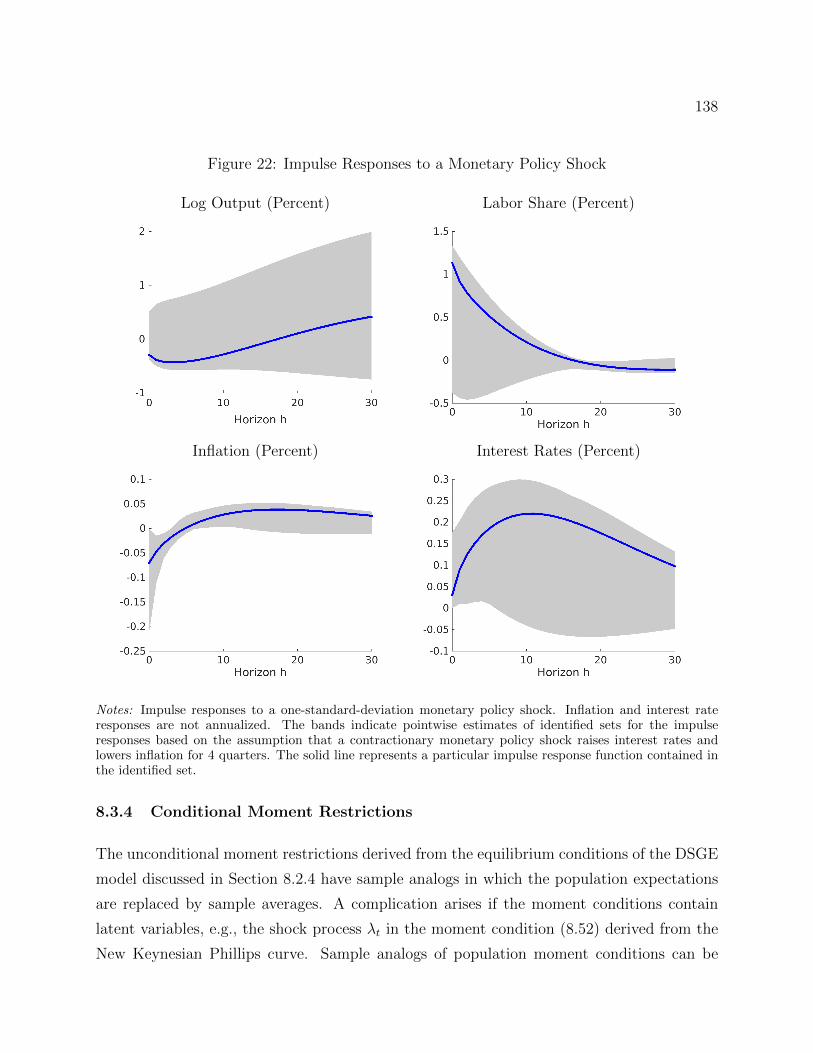
138

Figure 22: Impulse Responses to a Monetary Policy Shock

Log Output (Percent) Labor Share (Percent)

Inflation (Percent) Interest Rates (Percent)

Notes: Impulse responses to a one-standard-deviation monetary policy shock. Inflation and interest rateresponses are not annualized. The bands indicate pointwise estimates of identified sets for the impulseresponses based on the assumption that a contractionary monetary policy shock raises interest rates andlowers inflation for 4 quarters. The solid line represents a particular impulse response function contained inthe identified set.

8.3.4 Conditional Moment Restrictions

The unconditional moment restrictions derived from the equilibrium conditions of the DSGE

model discussed in Section 8.2.4 have sample analogs in which the population expectations

are replaced by sample averages. A complication arises if the moment conditions contain

latent variables, e.g., the shock process λt in the moment condition (8.52) derived from the

New Keynesian Phillips curve. Sample analogs of population moment conditions can be

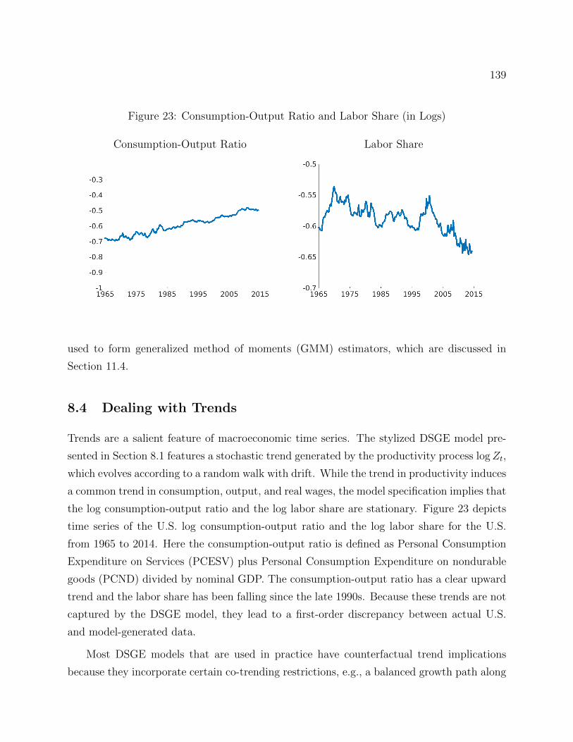
139

Figure 23: Consumption-Output Ratio and Labor Share (in Logs)

Consumption-Output Ratio Labor Share

used to form generalized method of moments (GMM) estimators, which are discussed in

Section 11.4.

8.4 Dealing with Trends

Trends are a salient feature of macroeconomic time series. The stylized DSGE model pre-

sented in Section 8.1 features a stochastic trend generated by the productivity process logZt,

which evolves according to a random walk with drift. While the trend in productivity induces

a common trend in consumption, output, and real wages, the model specification implies that

the log consumption-output ratio and the log labor share are stationary. Figure 23 depicts

time series of the U.S. log consumption-output ratio and the log labor share for the U.S.

from 1965 to 2014. Here the consumption-output ratio is defined as Personal Consumption

Expenditure on Services (PCESV) plus Personal Consumption Expenditure on nondurable

goods (PCND) divided by nominal GDP. The consumption-output ratio has a clear upward

trend and the labor share has been falling since the late 1990s. Because these trends are not

captured by the DSGE model, they lead to a first-order discrepancy between actual U.S.

and model-generated data.

Most DSGE models that are used in practice have counterfactual trend implications

because they incorporate certain co-trending restrictions, e.g., a balanced growth path along

140

which output, consumption, investment, the capital stock, and real wages exhibit a common

trend and hours worked and the return on capital are stationary, that are to some extent

violated in the data as we have seen in the above example. Researchers have explored

various remedies to address the mismatch between model and data, including: (i) detrending

each time series separately and fitting the DSGE model to detrended data; (ii) applying an

appropriate trend filter to both actual data and model-implied data when confronting the

DSGE model with data; (iii) creating a hybrid model, e.g., Canova (2014) that consists of

a flexible, non-structural trend component and uses the structural DSGE model to describe

fluctuations around the reduced-form trend; and (iv) incorporating more realistic trends

directly into the structure of the DSGE model. From a modeling perspective, option (i) is

the least desirable and option (iv) is the most desirable choice.

9 Statistical Inference

DSGE models have a high degree of theoretical coherence. This means that the functional

forms and parameters of equations that describe the behavior of macroeconomic aggregates

are tightly restricted by optimality and equilibrium conditions. In turn, the family of proba-

bility distributions p(Y |θ), θ ∈ Θ, generated by a DSGE model tends to be more restrictive

than the family of distributions associated with an atheoretical model, such as a reduced-

form VAR as in (8.60). This may place the empirical researcher in a situation in which the

data favor the atheoretical model and the atheoretical model generates more accurate fore-

casts, but a theoretically coherent model is required for the analysis of a particular economic

policy. The subsequent discussion of statistical inference will devote special attention to this

misspecification problem.

The goal of statistical inference is to infer an unknown parameter vector θ from observa-

tions Y ; to provide a measure of uncertainty about θ; and to document the fit of the statis-

tical model. The implementation of these tasks becomes more complicated if the statistical

model suffers from misspecification. Confronting DSGE models with data can essentially

take two forms. If it is reasonable to assume that the probabilistic structure of the DSGE

model is well specified, then one can ask how far the observed data Y o1:T or sample statistics

S(Y o1:T ) computed from the observed data fall into the tails of the model-implied distribution

derived from p(Y1:T |θ). The parameter vector θ can be chosen to ensure that the density

141

(likelihood) of S(Y o1:T ) is high under the distribution p(Y1:T |θ). If, on the other hand, there

is a strong belief (possibly supported by empirical evidence) that the probabilistic structure

of the DSGE model is not rich enough to capture the salient features of the observed data,

it is more sensible to consider a reference model with a well-specified probabilistic structure,

use it to estimate some of the population objects introduced in Section 8.2. and compare

these estimates to their model counterparts.

In Section 9.1 we ask the question whether the DSGE model parameters can be deter-

mined based on observations Y and review the recent literature on identification. We then

proceed by reviewing two modes of statistical inference: frequentist and Bayesian.37 We pay

special attention to the consequences of model misspecification. Frequentist inference, in-

troduced in Section 9.2, takes a pre-experimental perspective and focuses on the behavior of

estimators and test statistics, which are functions of the observations Y , in repeated sampling

under the distribution PYθ . Frequentist inference is conditioned on a “true” but unknown

parameter θ, or on a data-generating process (DGP), which is a hypothetical probability

distribution under which the data are assumed to be generated. Frequentist procedures have

to be well behaved for all values of θ ∈ Θ. Bayesian inference, introduced in Section 9.3,

takes a post-experimental perspective by treating the unknown parameter θ as a random

variable and updating a prior distribution p(θ) in view of the data Y using Bayes Theorem

to obtain the posterior distribution p(θ|Y ).

Estimation and inference requires that the model be solved many times for different

parameter values θ. The subsequent numerical illustrations are based on the stylized DSGE

model introduced in Section, for which we have a closed-form solution. However, such

closed-form solutions are the exception and typically not available for models used in serious

empirical applications. Thus, estimation methods, both frequentist and Bayesian, have to be

closely linked to model solution procedures. This ultimately leads to a trade-off: given a fixed

amount of computational resources, the more time is spent on solving a model conditional on

a particular θ, e.g., through the use of a sophisticated projection technique, the less often an

estimation objective function can be evaluated. For this reason, much of the empirical work

relies on first-order perturbation approximations of DSGE models, which can be obtained

very quickly. The estimation of models solved with numerically sophisticated projection

37A comparison between econometric inference approaches and the calibration approach advocated by Kyd-

land and Prescott (1982) can be found in Rıos-Rull, Schorfheide, Fuentes-Albero, Kryshko, and Santaeulalia-

Llopis (2012).

142

methods is relatively rare, because it requires a lot of computational resources. Moreover,

as discussed in Part I, perturbation solutions are more easily applicable to models with a

high-dimensional state vector and such models, in turn, are less prone to misspecification

and are therefore more easily amenable to estimation. However, the recent emergence of

low-cost parallel programming environments and cloud computing will make it feasible for a

broad group of researchers to solve and estimate elaborate non-linear DSGE models in the

near future.

9.1 Identification

The question of whether a parameter vector θ is identifiable based on a sample Y is of

fundamental importance for statistical inference because one of the main objectives is to

infer the unknown θ based on the sample Y . Suppose that the DSGE model generates a

family of probability distributions p(Y |θ), θ ∈ Θ. Moreover, imagine a stylized setting in

which data are in fact generated from the DSGE model conditional on some “true” parameter

θ0. The parameter vector θ0 is globally identifiable if

p(Y |θ) = p(Y |θ0) implies θ = θ0. (9.1)

The statement is somewhat delicate because it depends on the sample Y . From a pre-

experimental perspective, the sample is unobserved and it is required that (9.1) hold with

probability one under the distribution p(Y |θ0). From a post-experimental perspective, the

parameter θ may be identifiable for some trajectories Y , but not for others. The following

example highlights the subtle difference. Suppose that

y1,t|(θ, y2,t) ∼ iidN(θy2,t, 1

), y2,t =

0 w.p. 1/2

∼ iidN(0, 1) w.p. 1/2

Thus, with probability (w.p.) 1/2, one observes a trajectory along which θ is not identifiable

because y2,t = 0 for all t. If, on the other hand, y2,t 6= 0, then θ is identifiable.

9.1.1 Local Identification

If condition (9.1) is only satisfied for values of θ in an open neighborhood of θ0, then θ0

is locally identified. Most of the literature has focused on devising procedures to check

143

local identification in linearized DSGE models with Gaussian innovations. In this case the

distribution of Y |θ is a joint normal distribution and can be characterized by a Tny×1 vector

of means µ(θ) (where n is the dimension of the vector yt) and a Tny×Tny covariance matrix

Σ(θ). Defining m(θ) = [µ(θ)′, vech(Σ(θ))′]′, where vech(·) vectorizes the non-redundant

elements of a symmetric matrix, we can re-state the identification condition as

m(θ) = m(θ0) implies θ = θ0. (9.2)

Thus, verifying the local identification condition is akin to checking whether the Jacobian

J (θ) =∂

∂θ′m(θ) (9.3)

is of full rank. This approach was proposed and applied by Iskrev (2010) to examine the

identification of linearized DSGE models. If the joint distribution of Y is not Gaussian,

say because the DSGE model innovations εt are non-Gaussian or because the DSGE model

is non-linear, then it is possible that θ0 is not identifiable based on the first and second

moments m(θ), but that there are other moments that make it possible to distinguish θ0

from θ 6= θ0.

Local identification conditions are often stated in terms of the so-called information

matrix. Using Jensen’s inequality, it is straightforward to verify that the Kullback-Leibler

discrepancy between p(Y |θ0) and p(Y |θ) is non-negative:

∆KL(θ|θ0) = −∫

log

(p(Y |θ)p(Y |θ0)

)p(Y |θ0)dY ≥ 0. (9.4)

Under a non-degenerate probability distribution for Y , the relationship holds with equality

only if p(Y |θ) = p(Y |θ0). Thus, we deduce that the Kullback-Leibler distance is minimized

at θ = θ0 and that θ0 is identified if θ0 is the unique minimizer of ∆KL(θ|θ0). Let `(θ|Y ) =

log p(Y |θ) denote the log-likelihood function and ∇2θ`(θ|Y ) denote the matrix of second

derivatives of the log-likelihood function with respect to θ (Hessian), then (under suitable

regularity conditions that allow the exchange of integration and differentiation)

∇θ2∆KL(θ0|θ0) =

∫∇θ2`(θ0|Y )p(Y |θ0)dY. (9.5)

In turn, the model is locally identified at θ0 if the expected Hessian matrix is non-singular.

For linearized Gaussian DSGE models that can be written in the form Y ∼ N(µ(θ),Σ(θ)

)we obtain ∫

∇2θ`(θ0|Y )p(Y |θ0)dY = J (θ)′ΩJ (θ), (9.6)

144

where Ω is the Hessian matrix associated with the unrestricted parameter vector m =

[µ′, vech(Σ)′]′ of a N(µ,Σ). Because Ω is a symmetric full-rank matrix of dimension dim(m),

we deduce that the Hessian is of full rank whenever the Jacobian matrix in (9.3) is of full

rank.

Qu and Tkachenko (2012) focus on the spectral density matrix of the process yt. Using

a frequency domain approximation of the likelihood function and utilizing the information

matrix equality, they express the Hessian as the outer product of the Jacobian matrix of

derivatives of the spectral density with respect to θ

G(θ0) =

∫ π

−π

(∂

∂θ′vec(fyy(ω)′)

)′(∂

∂θ′vec(fyy(ω))

)dω (9.7)

and propose to verify whether G(θ0) is of full rank. The identification checks of Iskrev (2010)

and Qu and Tkachenko (2012) have to be implemented numerically. For each conjectured

θ0 the user has to compute the rank of the matrices J (θ0) or G(θ0), respectively. Because

in a typical implementation the computation of the matrices relies on numerical differen-

tiation (and integration), careful attention has be paid to the numerical tolerance level of

the procedure that computes the matrix rank. Detailed discussions can be found in the two

referenced papers.

Komunjer and Ng (2011) take a different route to assess the local identification of lin-

earized DSGE models. They examine the relationship between the coefficients of the state-

space representation of the DSGE model and the parameter vector θ. Recall that the state-

space representation takes the form

yt = Ψ0(θ) + Ψ1(θ), st = Φ1(θ)st−1 + Φε(θ)εt. (9.8)

The notation highlights the dependence of the coefficient matrices on θ. Now stack the

coefficients of the Ψ and Φ matrices in the vector φ:

φ =[vec(Ψ0)′, vec(Ψ1)′, vec(Φ1)′, vec(Φε)

′]′.It is tempting to conjecture that θ is locally identifiable if the Jacobian matrix associated

with the mapping from economic parameters θ to the reduced-form state-space parameters

φ∂

∂θ′φ(θ) (9.9)

145

has full column rank at θ0. The problem with this conjecture is that the reduced-form

parameters φ themselves are not identifiable. Let A be a non-singular ns× ns matrix and Ω

an nε × nε orthogonal matrix, then we can define

st = Ast, εt = Ωεt, Ψ1 = Ψ1A−1, Φ1 = Φ1A

−1, Φε = AΦεΩ′

to obtain an observationally equivalent state-space system

yt = Ψ0 + Ψ1st, st = Φ1st−1 + Φεεt (9.10)

with φ 6= φ. Thus, the number of identifiable reduced-form parameters is smaller than the

number of elements in the Ψ and Φ matrices. The main contribution in Komunjer and Ng

(2011) is to account for the non-identifiability of the reduced-form state-space parameters

when formulating a rank condition along the lines of (9.9). In many DSGE models a subset

of the state transitions are deterministic, which complicates the formal analysis.

Identification becomes generally more tenuous the fewer variables are included in the

vector yt. For instance, in the context of the stylized DSGE model, suppose yt only includes

the labor share. According to (8.17) the law of motion for the labor share is the sum of three

AR(1) processes and an iid monetary policy shock. It can be rewritten as an ARMA(3,3)

process and therefore has at most 8 identifiable reduced-form parameters. Thus, the upper

bound on the number of reduced-form parameters is less than the number of DSGE model

parameters, which is 13. In turn, it is not possible to identify the entire θ vector.

9.1.2 Global Identification

Global identification is more difficult to verify than local identification. Consider the follow-

ing example from Schorfheide (2013):

yt = [1 1]st, st =

[θ2

1 0

1− θ21 − θ1θ2 (1− θ2

1)

]st−1 +

[1

0

]εt, εt ∼ iidN(0, 1). (9.11)

Letting L denote the lag operator with the property that Lyt = yt−1, one can write the law

of motion of yt as an restricted ARMA(2,1) process:(1− θ2

1L)(

1− (1− θ21)L)yt =

(1− θ1θ2L

)εt. (9.12)

146

It can be verified that given θ1 and θ2, an observationally equivalent process can be obtained

by choosing θ1 and θ2 such that

θ1 =√

1− θ21, θ2 = θ1θ2/θ1.

Here we switched the values of the two roots of the autoregressive lag polynomial. Qu and

Tkachenko (2014) propose to check for global identification by searching for solutions to the

equation

0 = ∆KL(θ|θ0), θ ∈ Θ. (9.13)

If θ0 is the unique solution, then the DSGE model is globally identified. The authors evaluate

the Kullback-Leibler discrepancy using a frequency domain transformation. The computa-

tional challenge is to find all the roots associated with (9.13). Kociecki and Kolasa (2015)

follow a slightly different approach that is attractive because it requires the user to solve the

DSGE model only at θ0, but not at all the other values of θ ∈ Θ.

9.2 Frequentist Inference

The fundamental problem of statistical inference is to infer the parameter vector θ, in our case

the DSGE model parameters, based on a random sample Y . Frequentist inference adopts a

pre-experimental perspective and examines the sampling distribution of estimators and test

statistics, which are transformations of the random sample Y , conditional on a hypothetical

DGP. We will distinguish between two cases. First, we consider the stylized case in which

the DSGE model is correctly specified. Formally, this means that Y is sampled from p(Y |θ0),

where the density p(Y |θ0) is derived from the DSGE model and θ is the “true” but unknown

parameter vector.38 Second, we consider the case of misspecification, meaning the DSGE

model is too stylized to capture some of the key features of the data Y . As a consequence,

the sampling distribution of Y has to be characterized by a reference model, for instance,

a VAR or a linear process. In terms of notation, we will distinguish between the DSGE

model, denoted by M1, and the reference model M0. To avoid confusion about which model

generates the sampling distribution of Y , we add the model indicator to the conditioning set

and write, e.g., p(Y |θ,M1) or p(Y |M0). We also use the notation ‖a‖W = a′Wa.

38In reality, of course, the observed Y is never generated from a probabilistic mechanism. Instead it

reflects measured macroeconomic activity. Thus, by “correct specification of a DSGE model” we mean that

we believe that its probabilistic structure is rich enough to assign high probability to the salient features of

macroeconomic time series.

147

9.2.1 “Correct” Specification of DSGE Model

Under the assumption of correct specification, the DSGE model itself is the DGP and

p(Y |θ0,M1) describes the sampling distribution of Y under which the behavior of estimators

and test statistics is being analyzed. In this case it is desirable to let the model-implied

probability distribution p(Y |θ0,M1) determine the choice of the objective function for esti-

mators and test statistics to obtain a statistical procedure that is efficient (meaning that

the estimator is close to θ0 with high probability in repeated sampling). In this regard, the

maximum likelihood (ML) estimator

θml = argmaxθ∈Θ log p(Y |θ,M1) (9.14)

plays a central role in frequentist inference, because it is efficient under fairly general regu-

larity conditions. One of these conditions is that θ0 is identifiable.

Alternative estimators can be obtained by constructing an objective function QT (θ|Y )

that measures the discrepancy between sample statistics mT (Y ) (see Section 8.3) and model-

implied population statistics E[mT (Y )|θ,M1] (see Section 8.2). Examples of the vector

mT (Y ) are, for instance, vectorized sample autocovariances such as

mT (Y ) =[vech(Γyy(0))′, vec(Γyy(1))′

]=

1

T

T∑t=1

m(yt−1:t)

or the OLS estimator of the coefficients of a VAR(1) (here without intercept)

mT (Y ) = vec

( 1

T

T∑t=1

yt−1y′t−1

)−1

1

T

T∑t=1

yt−1y′t

.

We write the estimation objective function as

QT (θ|Y ) =∥∥mT (Y )− E[mT (Y )|θ,M1]

∥∥WT, (9.15)

whereWT is a symmetric positive-definite weight matrix. Under the assumption of a correctly

specified DSGE model, the optimal choice of the weight matrix WT is the inverse of the

DSGE model-implied covariance matrix of mT (Y ). Thus, more weight is assigned to sample

moments that accurately approximate the underlying population moment. The minimum

distance (MD) estimator of θ is defined as

θmd = argmaxθ∈Θ QT (θ|Y ). (9.16)

148

Econometric inference is based on the sampling distribution of the estimator θmd and confi-

dence sets and test statistics derived from θmd andQT (θ|Y ) under the distribution p(Y |θ0,M1).

9.2.2 Misspecification and Incompleteness of DSGE Models

Model misspecification can be interpreted as a violation of the cross-coefficient restrictions

embodied in the mapping from the DSGE model parameters θ into the system matrices Ψ0,

Ψ1, Φ1, and Φε of the state-space representation in (8.23) and (8.25). An example of an

incomplete model is a version of the stylized DSGE model in which we do not fully specify

the law of motion for the exogenous shock processes and restrict our attention to certain

moment conditions, such as the consumption Euler equation. In some cases, incompleteness

and misspecification are two sides of the same coin. Consider a version of the stylized DSGE

model with only one structural shock, namely, the monetary policy shock. This version does

not contain sufficiently many shocks to explain the observed variability in output growth, the

labor share, inflation, and the interest rate. More specifically, the one-shock DSGE model

implies, for instance, that the linear combination

1

κp(1 + ν)xεR/β + σRRt −

1

κp(1 + ν)xεRπt = 0

is perfectly predictable; see (8.19) and (8.20). This prediction is clearly counterfactual. We

could regard the model as misspecified, in the sense that its predictions are at odds with the

data; or as incomplete, in the sense that adding more structural shocks could reduce the gap

between model and reality.

Regardless of whether the DSGE model is incomplete or misspecificed, it does not pro-

duce a sampling distribution for the data Y that can be used to determine the frequentist

behavior of estimators and test statistics. In order to conduct a frequentist analysis, we

require a reference model M0 that determines the distribution of the data p(Y |M0) and can

be treated as a DGP. The reference model could be a fully specified parametric model such

as a VAR, p(Y |φ,M0), where φ is a finite-dimensional parameter vector. Alternatively, the

reference model could be a general stochastic process for yt that satisfies a set of regularity

conditions necessary to establish large sample approximations to the sampling distributions

of estimators and test statistics.

149

If the DSGE model is incompletely specified, it is still possible to uphold the notion of a

“true” parameter vector θ0, in the sense that one could imagine the DGP to be the incom-

pletely specified DSGE model augmented by a set of equations (potentially with additional

parameters). If the DSGE model is misspecified, then the concept of a “true” parameter

value has to be replaced by the notion of a pseudo-true (or pseudo-optimal) parameter value.

The definition of a pseudo-true parameter value requires a notion of discrepancy between

the DGP p(Y |M0) and the DSGE model p(Y |θ,M1). Different discrepancies lead to different

pseudo-optimal values. Likelihood-based inference is associated with the Kullback-Leibler

discrepancy and would lead to

θ0(KL) = argminθ∈Θ −∫

log

(p(Y |θ,M1)

p(Y |M0)

)p(Y |M0)dY. (9.17)

Moment-based inference based on the sample objective function QT (θ|Y ) is associated with

a pseudo-optimal value

θ0(Q,W ) = argminθ∈Θ Q(θ|M0), (9.18)

where

Q(θ|M0) =∥∥E[mT (Y )|M0]− E[m(Y )|θ,M1]

∥∥W.

Ultimately, the sampling properties of estimators and test statistics have to be derived from

the reference model M0.

9.3 Bayesian Inference

Under the Bayesian paradigm, the calculus of probability is used not only to deal with uncer-

tainty about shocks εt, states st, and observations yt, but also to deal with uncertainty about

the parameter vector θ. The initial state of knowledge (or ignorance) is summarized by a

prior distribution with density p(θ). This prior is combined with the conditional distribution

of the data given θ, i.e., the likelihood function, to characterize the joint distribution of

parameters and data. Bayes Theorem is applied to obtain the conditional distribution of the

parameters given the observed data Y . This distribution is called the posterior distribution:

p(θ|Y,M1) =p(Y |θ,M1)p(θ|M1)

p(Y |M1), p(Y |M1) =

∫p(Y |θ,M1)p(θ|M1)dθ. (9.19)

The posterior distribution contains all the information about θ conditional on sample infor-

mation Y . In a Bayesian setting a model comprises the likelihood function p(Y |θ,M1) and

the prior p(θ|M1).

150

The posterior distribution of transformations of the DSGE model parameters θ, say,

h(θ), e.g., autocovariances and impulse response functions, can be derived from p(θ|Y,M1).

For instance,

PY h(θ) ≤ h =

∫θ | h(θ)≤h

p(θ|Y,M1)dθ. (9.20)

Solution to inference problems can generally be obtained by specifying a suitable loss func-

tion, stating the inference problem as a decision problem, and minimizing posterior expected

loss. For instance, to obtain a point estimator for h(θ), let L(h(θ), δ

)describe the loss asso-

ciated with reporting δ if h(θ) is correct. The optimal decision δ∗ is obtained by minimizing

the posterior expected loss:

δ∗ = argminδ∈D

∫L(h(θ), δ

)p(θ|Y,M1)dθ. (9.21)

If the loss function is quadratic, then the optimal point estimator is the posterior mean of

h(θ).

The most difficult aspect of Bayesian inference is the characterization of the posterior

moments of h(θ). Unfortunately, it is not possible to derive these moments analytically

for DSGE models. Thus, researchers have to rely on numerical methods. The Bayesian

literature has developed a sophisticated set of algorithms to generate draws θi from the

posterior distribution, such that averages of these draws converge to posterior expectations:

E[h(θ)|Y,M1] =

∫h(θ)p(θ|Y,M1)dθ ≈ 1

N

N∑i=1

h(θi). (9.22)

Several of these computational techniques are discussed in more detail in Section 12.

9.3.1 “Correct” Specification of DSGE Models

The use of Bayes Theorem to learn about the DSGE model parameters implicitly assumes

that the researcher regards the probabilistic structure of the DSGE model as well specified in

the sense that there are parameters θ in the support of the prior distribution conditional on

which the salient features of the data Y are assigned a high probability. Of course, in practice

there is always concern that an alternative DSGE model may deliver a better description of

the data. The Bayesian framework is well suited to account for model uncertainty.

Suppose the researcher contemplates two model specifications M1 and M2, assuming that

one of them is correct. It is natural to place prior probabilities on the two models, which we

151

denote by πj,0. Ratios of model probabilities are called model odds. The posterior odds of

M1 versus M2 are given byπ1,T

π2,T

=π1,0

π2,0

p(Y |M1)

p(Y |M2), (9.23)

where the first factor on the right-hand side captures the prior odds and the second factor,

called Bayes factor, is the ratio of marginal data densities. Note that p(Y |Mi) appears in

the denominator of Bayes Theorem (9.19). Posterior model odds and probabilities have been

widely used in the DSGE model literature to compare model specification or to take averages

across DSGE models. Prominent applications include Rabanal and Rubio-Ramırez (2005)

and Smets and Wouters (2007).

9.3.2 Misspecification of DSGE Models

As in the frequentist case, model misspecification complicates inference. Several approaches

have been developed in the literature to adapt Bayesian analysis to the potential misspec-

ification of DSGE models. In general, the model space needs to be augmented by a more

densely parameterized reference model, M0, that provides a more realistic probabilistic rep-

resentation of the data.

Schorfheide (2000) considers a setting in which a researcher is interested in the relative

ability of two (or more) DSGE models, say, M1 and M2, to explain certain population

characteristics ϕ, e.g., autocovariances or impulse responses.39 However, the DSGE models

may be potentially misspecified and the researcher considers a reference model M0. As long

as it is possible to form a posterior distribution for ϕ based on the reference model, the

overall posterior can be described by

p(ϕ|Y ) =∑j=0,1,2

πj,Tp(ϕ|Y,Mj). (9.24)

If one of the DSGE models is well specified, this model receives high posterior probability

and dominates the mixture. If both DSGE models are at odds with the data, the posterior

probability of the reference model will be close to one. Given a loss function over predictions

of ϕ, one can compute DSGE model-specific predictions:

ϕ(j) = argminϕ

∫L(ϕ, ϕ)p(ϕ|Y,Mj)dϕ, j = 1, 2. (9.25)

39Frequentist versions of this approach have been developed in Hnatkosvaka, Marmer, and Tang (2012)

and Marmer and Otsu (2012).

152

Finally, the two DSGE models can be ranked based on the posterior risk∫L(ϕ(j), ϕ)p(ϕ|Y )dϕ. (9.26)

Geweke (2010) assumes that the researcher regards the DSGE models not as models of

the data Y , but as models of some population moments ϕ. A reference model M0, e.g., a

VAR, provides the model for Y , but also permits the computation of implied population

moments. He shows that under these assumptions, one can define the posterior odds of

DSGE models asπ1,T

π2,T

=π1,0

π2,0

∫p(ϕ|M1)p(ϕ|Y,M0)dϕ∫p(ϕ|M2)p(ϕ|Y,M0)dϕ

. (9.27)

Roughly, if we were able to observe ϕ, then p(ϕ|Mj) is the marginal likelihood. However, ϕ

is unobservable and therefore replaced by a posterior predictive distribution obtained from

a reference model M0. The odds in favor of model M1 are high if there is a lot of overlap

between the preditive distribution for the population moments ϕ under the DSGE model,

and the posterior distribution of ϕ obtained when estimating the reference model M0.

Building on work by Ingram and Whiteman (1994), Del Negro and Schorfheide (2004)

do not treat the DSGE model as a model of the data Y , but instead use it to construct a

prior distribution for a VAR. Consider the companion form VAR in (8.61). Use the DSGE

model to generate a prior distribution for (Φ1, Φ0, Σ) and combine this prior with the VAR

likelihood function

p(Y, Φ0, Φ1, Σ, θ|λ) = p(Y |Φ0, Φ1, Σ)p(Φ0, Φ1, Σ|θ, λ)p(θ). (9.28)

The resulting hierarchical model is called a DSGE-VAR. The prior p(Φ0, Φ1, Σ|θ, λ) is cen-

tered on restriction functions

Φ∗0(θ), Φ∗1(θ), Σ∗(θ),

but allows for deviations from these restriction functions to account for model misspecifica-

tion. The parameter λ is a hyperparameter that controls the magnitude of the deviations

(prior variance) from the restriction function. This framework can be used for forecasting,

to assess the fit of DSGE models, e.g., Del Negro, Schorfheide, Smets, and Wouters (2007),

and to conduct policy analysis, e.g., Del Negro and Schorfheide (2009).

In a setting in which the reference model M0 plays a dominating role, Fernandez-

Villaverde and Rubio-Ramırez (2004) show that choosing the DSGE model that attains

153

the highest posterior probability (among, say, competing DSGE models M1 and M2) leads

asymptotically to the specification that is closest to M0 in a Kullback-Leibler sense. Rather

than using posterior probabilities to select among or average across two DSGE models, one

can form a prediction pool, which is essentially a linear combination of two predictive den-

sities:

λp(yt|Y1:t−1,M1) + (1− λ)p(yt|Y1:t−1,M2).

The weight λ ∈ [0, 1] can be determined based on

T∏t=1

[λp(yt|Y1:t−1,M1) + (1− λ)p(yt|Y1:t−1,M2)] .

This objective function could either be maximized with respect to λ or it can be treated

as a likelihood function for λ and embedded in a Bayesian inference procedure. This idea

is developed in Geweke and Amisano (2011) and Geweke and Amisano (2012). Dynamic

versions with λ depending on time t are provided by Waggoner and Zha (2012) and Del Negro,

Hasegawa, and Schorfheide (2014).

10 The Likelihood Function

The likelihood function plays a central role in both frequentist and Bayesian inference. The

likelihood function treats the joint density of the observables conditional on the parameters,

p(Y1:T |θ), as a function of θ. The state-space representation of the DSGE model leads to

a joint distribution p(Y1:T , S1:T |θ); see (8.26). In order to obtain the likelihood function,

one needs to integrate out the (hidden) states S1:T . This can be done recursively, using an

algorithm that is a called a filter.

This section focuses on the numerical evaluation of the likelihood function conditional on

a particular parameterization θ through the use of linear and non-linear filters. We assume

that the DSGE model has the following, possibly non-linear, state-space representation:

yt = Ψ(st, t; θ) + ut, ut ∼ Fu(·; θ) (10.1)

st = Φ(st−1, εt; θ), εt ∼ Fε(·; θ).

The state-space system is restricted in two dimensions. First, the errors in the measurement

equation enter in an additively separable manner. This implies that the conditional density

154

p(yt|st, θ) is given by pu(yt −Ψ(st, t; θ)|θ

), where pu(·|θ) is the pdf associated with the mea-

surement error distribution Fu(·; θ). In the absence of measurement errors, the distribution

yt|(st, θ) is a pointmass at Ψ(st, t; θ). Second, the state-transition equation has a first-order

Markov structure.40 Owing to the first-order Markov structure of the state-transition equa-

tion, neither the states st−2, st−3, . . . nor the observations yt−1, yt−2, . . . provide any additional

information about st conditional on st−1. Thus,

p(st|st−1, θ) = p(st|st−1, S1:t−2, θ) = p(st|st−1, S1:t−2, Y1:t−1, θ). (10.2)

For the linearized DSGE model of Section 8.1 with normally distributed measurement errors

ut ∼ N(0,Σu) the conditional distributions are given by st|(st−1, θ) ∼ N(Φ1st−1,ΦεΦ

′ε

)and

yt|(st, θ) ∼ N(Ψ0 + Ψ1st,Σu).

10.1 A Generic Filter

We now describe a generic filter that can be used to recursively compute the conditional

distributions p(st|Y1:t, θ) and p(yt|Y1:t−1, θ), starting from an initialization p(s0|θ). The dis-

tributions p(st|Y1:t, θ) are a by-product of the algorithm and summarize the information

about the state st conditional on the current and past observations Y1:t, which may be of

independent interest. The sequence of predictive distributions p(yt|Y1:t−1, θ), t = 1, . . . , T ,

can be used to obtain the likelihood function, which can be factorized as follows

p(Y1:T |θ) =T∏t=1

p(yt|Y1:t−1, θ). (10.3)

The filter is summarized in Algorithm 5. In the description of the filter we drop the parameter

θ from the conditioning set to simplify the notation.

Algorithm 5 (Generic Filter).

Let p(s0) = p(s0|Y1:0) be the initial distribution of the state. For t = 1 to T :

1. Forecasting t given t− 1:

40Additional lags of the state vector could be easily incorporated using a companion form representation

of the state vector as in (8.61).

155

(a) Transition equation:

p(st|Y1:t−1) =

∫p(st|st−1, Y1:t−1)p(st−1|Y1:t−1)dst−1

(b) Measurement equation:

p(yt|Y1:t−1) =

∫p(yt|st, Y1:t−1)p(st|Y1:t−1)dst

2. Updating with Bayes Theorem. Once yt becomes available:

p(st|Y1:t) = p(st|yt, Y1:t−1) =p(yt|st, Y1:t−1)p(st|Y1:t−1)

p(yt|Y1:t−1).

10.2 Likelihood Function for a Linearized DSGE Model

For illustrative purposes, consider the prototypical DSGE model. Owing to the simple

structure of the model, we can use (8.16), (8.17), (8.19), and (8.20) to solve for the latent

shocks φt, λt, zt, and εR,t as a function of xt, lsht, πt, and Rt. Thus, we can deduce from (8.25)

and the definition of st that conditional on x0, the states st can be uniquely inferred from the

observables yt in a recursive manner, meaning that the conditional distributions p(st|Y1:t, x0)

are degenerate. Thus, the only uncertainty about the state stems from the initial condition.

Suppose that we drop the labor share and the interest rates from the definition of yt. In

this case it is no longer possible to uniquely determine st as a function of yt and x0, because

we only have two equations, (8.16) and (8.19), and four unknowns. The filter in Algorithm 5

now essentially solves an underdetermined system of equations, taking into account the

probability distribution of the four hidden processes. For our linearized DSGE model with

Gaussian innovations, all the distributions that appear in Algorithm 5 are Gaussian. In

this case the Kalman filter can be used to compute the means and covariance matrices of

these distributions recursively. To complete the model specification, we make the following

distributional assumptions about the initial state s0:

s0 ∼ N(s0|0, P0|0

).

In stationary models it is common to set s0|0 and P0|0 equal to the unconditional first and

second moments of the invariant distribution associated with the law of motion of st in (8.23).

The four conditional distributions in the description of Algorithm 5 for a linear Gaussian

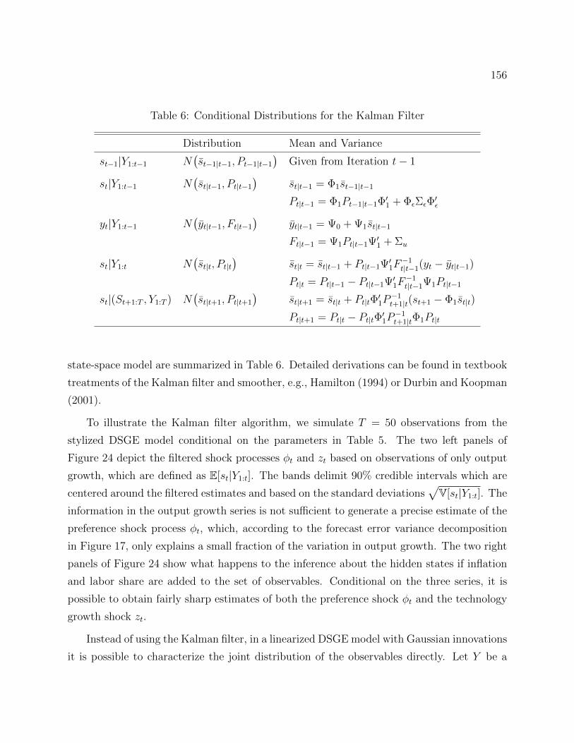
156

Table 6: Conditional Distributions for the Kalman Filter

Distribution Mean and Variance

st−1|Y1:t−1 N(st−1|t−1, Pt−1|t−1

)Given from Iteration t− 1

st|Y1:t−1 N(st|t−1, Pt|t−1

)st|t−1 = Φ1st−1|t−1

Pt|t−1 = Φ1Pt−1|t−1Φ′1 + ΦεΣεΦ′ε

yt|Y1:t−1 N(yt|t−1, Ft|t−1

)yt|t−1 = Ψ0 + Ψ1st|t−1

Ft|t−1 = Ψ1Pt|t−1Ψ′1 + Σu

st|Y1:t N(st|t, Pt|t

)st|t = st|t−1 + Pt|t−1Ψ′1F

−1t|t−1(yt − yt|t−1)

Pt|t = Pt|t−1 − Pt|t−1Ψ′1F−1t|t−1Ψ1Pt|t−1

st|(St+1:T , Y1:T ) N(st|t+1, Pt|t+1

)st|t+1 = st|t + Pt|tΦ

′1P−1t+1|t(st+1 − Φ1st|t)

Pt|t+1 = Pt|t − Pt|tΦ′1P−1t+1|tΦ1Pt|t

state-space model are summarized in Table 6. Detailed derivations can be found in textbook

treatments of the Kalman filter and smoother, e.g., Hamilton (1994) or Durbin and Koopman

(2001).

To illustrate the Kalman filter algorithm, we simulate T = 50 observations from the

stylized DSGE model conditional on the parameters in Table 5. The two left panels of

Figure 24 depict the filtered shock processes φt and zt based on observations of only output

growth, which are defined as E[st|Y1:t]. The bands delimit 90% credible intervals which are

centered around the filtered estimates and based on the standard deviations√

V[st|Y1:t]. The

information in the output growth series is not sufficient to generate a precise estimate of the

preference shock process φt, which, according to the forecast error variance decomposition

in Figure 17, only explains a small fraction of the variation in output growth. The two right

panels of Figure 24 show what happens to the inference about the hidden states if inflation

and labor share are added to the set of observables. Conditional on the three series, it is

possible to obtain fairly sharp estimates of both the preference shock φt and the technology

growth shock zt.

Instead of using the Kalman filter, in a linearized DSGE model with Gaussian innovations

it is possible to characterize the joint distribution of the observables directly. Let Y be a

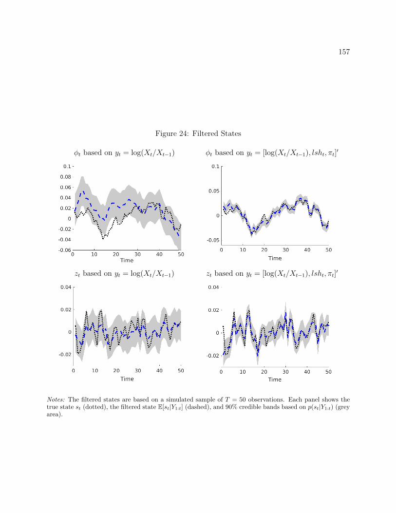
157

Figure 24: Filtered States

φt based on yt = log(Xt/Xt−1) φt based on yt = [log(Xt/Xt−1), lsht, πt]′

zt based on yt = log(Xt/Xt−1) zt based on yt = [log(Xt/Xt−1), lsht, πt]′

Notes: The filtered states are based on a simulated sample of T = 50 observations. Each panel shows thetrue state st (dotted), the filtered state E[st|Y1:t] (dashed), and 90% credible bands based on p(st|Y1:t) (greyarea).

158

T × ny matrix composed of rows y′t. Then the joint distribution of Y is given by

vec(Y )|θ ∼ N

I ⊗ Φ0(θ),

Γyy(0|θ) Γyy(1|θ) . . . Γyy(T − 1|θ)Γ′yy(1|θ) Γyy(0|θ) . . . Γyy(T − 2|θ)

......

. . ....

Γ′yy(T − 1|θ) Γ′yy(T − 2|θ) . . . Γyy(0|θ)

. (10.4)

The evaluation of the likelihood function requires the calculation of the autocovariance se-

quence and the inversion of an nyT × nyT matrix. For large T the joint density can be

approximated by the so-called Whittle likelihood function

pW (Y |θ) ∝(T−1∏j=0

∣∣2πf−1yy (ωj|θ)

∣∣)1/2

exp

−1

2

T−1∑j=0

tr[f−1yy (ωj|θ)fyy(ωj)

](10.5)

where fyy(ω|θ) is the DSGE model-implied spectral density, fyy(ω) is the sample peri-

odogram, and the ωj’s are the fundamental frequencies. The attractive feature of this

likelihood function is that the researcher can introduce weights for the different frequen-

cies, and, for instance, only consider business cycle frequencies in the construction of the

likelihood function. For the estimation of DSGE models, the Whittle likelihood has been

used, for instance, by Christiano and Vigfusson (2003), Qu and Tkachenko (2012), and Sala

(2015).

10.3 Likelihood Function for Non-linear DSGE Models

If the DSGE model is solved using a non-linear approximation technique, then either the

state-transition equation, or the measurement equation, or both become non-linear. As

a consequence, analytical representations of the densities p(st−1|Y1:t−1), p(st|Y1:t−1), and

p(yt|Y1:t−1) that appear in Algorithm 5 are no longer available. While there exists a large

literature on non-linear filtering (see for instance Crisan and Rozovsky (2011)) we focus on

the class of particle filters. Particle filters belong to the class of sequential Monte Carlo

algorithms. The basic idea is to approximate the distribution st|Y1:t through a swarm of

particles sjt ,W jt Mj=1 such that

ht,M =1

M

M∑j=1

h(sjt)Wjt

a.s.−→ E[h(st)|Y1:t], (10.6)

√M(ht,M − E[h(st)|Y1:t]

)=⇒ N

(0,Ωt[h]

),

159

where =⇒ denotes convergence in distribution.41 Here the sjt ’s are particle values and the

W jt ’s are the particle weights. The conditional expectation of h(st) is approximated by

a weighted average of the (transformed) particles h(sjt). Under suitable regularity condi-

tions, the Monte Carlo approximation satisfies an SLLN and a CLT. The covariance ma-

trix Ωt[h] characterizes the accuracy of the Monte Carlo approximation. Setting h(st) =

p(yt+1|st) yields the particle filter approximation of the likelihood increment p(yt+1|Y1:t) =

E[p(yt+1|st)|Y1:t]. Each iteration of the filter manipulates the particle values and weights to

recursively track the sequence of conditional distributions st|Y1:t. The paper by Fernandez-

Villaverde and Rubio-Ramırez (2007) was the first to approximate the likelihood function

of a non-linear DSGE model using a particle filter and many authors have followed this

approach.

Particle filters are widely used in engineering and statistics. Surveys and tutorials are

provided, for instance, in Arulampalam, Maskell, Gordon, and Clapp (2002), Cappe, Godsill,

and Moulines (2007), Doucet and Johansen (2011), and Creal (2012). The basic bootstrap

particle filter algorithm is remarkably straightforward, but may perform quite poorly in

practice. Thus, much of the literature focuses on refinements of the bootstrap filter that

increases the efficiency of the algorithm; see, for instance, Doucet, de Freitas, and Gordon

(2001). Textbook treatments of the statistical theory underlying particle filters can be found

in Cappe, Moulines, and Ryden (2005), Liu (2001), and Del Moral (2013).

10.3.1 Generic Particle Filter

The subsequent exposition draws from Herbst and Schorfheide (2015), who provide a detailed

presentation of particle filtering techniques in the context of DSGE model applications as

well as a more extensive literature survey. In the basic version of the particle filter, the

time t particles are generated based on the time t − 1 particles by simulating the state-

transition equation forward. The particle weights are then updated based on the likelihood

of the observation yt under the sjt particle, p(yt|sjt). The more accurate the prediction of yt

based on sjt , the larger the density p(yt|sjt), and the larger the relative weight that will be

placed on particle j. However, the naive forward simulation ignores information contained in

the current observation yt and may lead to a very uneven distribution of particle weights, in

41A sequence of random variables XT converges in distribution to a random variable X if for every

measurable and bounded function f(·) that is continuous almost everywhere E[f(XT )] −→ E[f(X)].

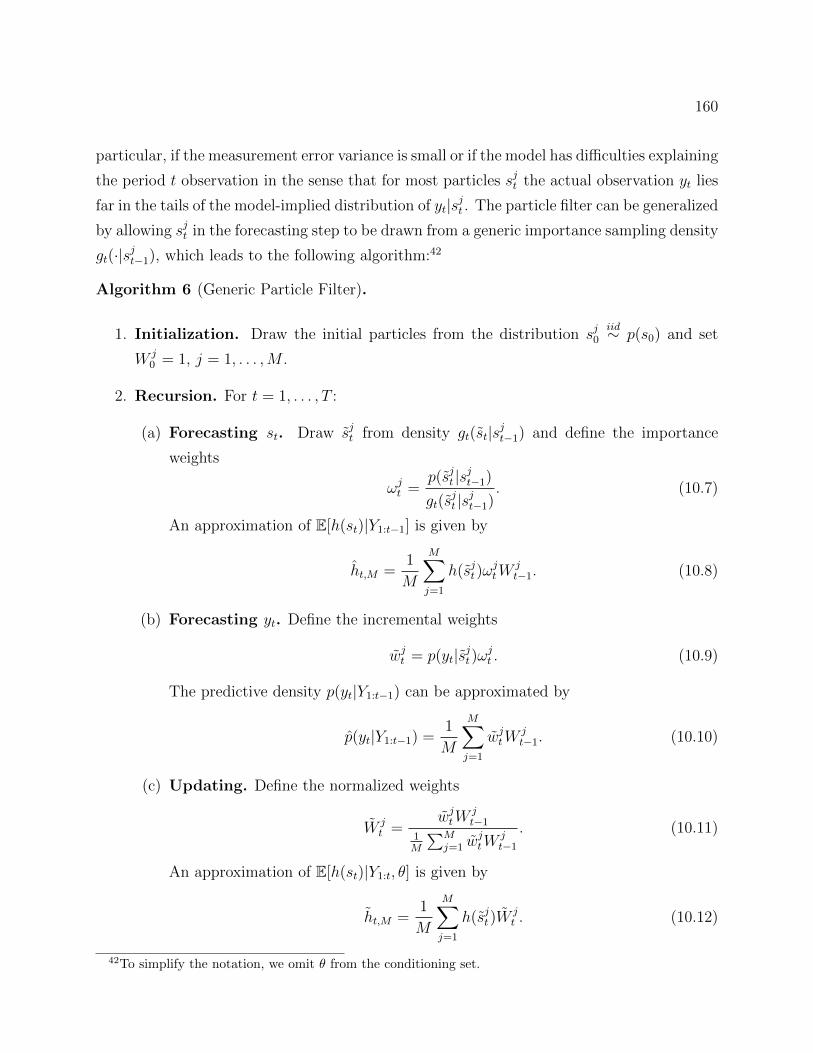
160

particular, if the measurement error variance is small or if the model has difficulties explaining

the period t observation in the sense that for most particles sjt the actual observation yt lies

far in the tails of the model-implied distribution of yt|sjt . The particle filter can be generalized

by allowing sjt in the forecasting step to be drawn from a generic importance sampling density

gt(·|sjt−1), which leads to the following algorithm:42

Algorithm 6 (Generic Particle Filter).

1. Initialization. Draw the initial particles from the distribution sj0iid∼ p(s0) and set

W j0 = 1, j = 1, . . . ,M .

2. Recursion. For t = 1, . . . , T :

(a) Forecasting st. Draw sjt from density gt(st|sjt−1) and define the importance

weights

ωjt =p(sjt |sjt−1)

gt(sjt |sjt−1)

. (10.7)

An approximation of E[h(st)|Y1:t−1] is given by

ht,M =1

M

M∑j=1

h(sjt)ωjtW

jt−1. (10.8)

(b) Forecasting yt. Define the incremental weights

wjt = p(yt|sjt)ωjt . (10.9)

The predictive density p(yt|Y1:t−1) can be approximated by

p(yt|Y1:t−1) =1

M

M∑j=1

wjtWjt−1. (10.10)

(c) Updating. Define the normalized weights

W jt =

wjtWjt−1

1M

∑Mj=1 w

jtW

jt−1

. (10.11)

An approximation of E[h(st)|Y1:t, θ] is given by

ht,M =1

M

M∑j=1

h(sjt)Wjt . (10.12)

42To simplify the notation, we omit θ from the conditioning set.

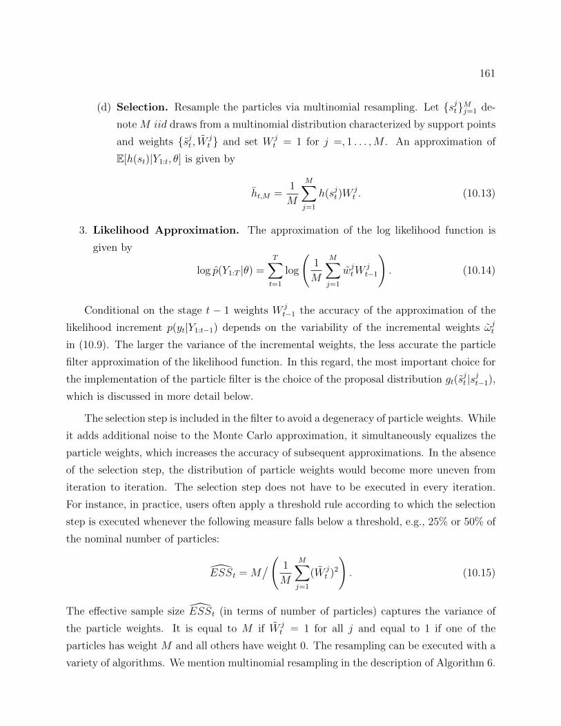
161

(d) Selection. Resample the particles via multinomial resampling. Let sjtMj=1 de-

note M iid draws from a multinomial distribution characterized by support points

and weights sjt , W jt and set W j

t = 1 for j =, 1 . . . ,M . An approximation of

E[h(st)|Y1:t, θ] is given by

ht,M =1

M

M∑j=1

h(sjt)Wjt . (10.13)

3. Likelihood Approximation. The approximation of the log likelihood function is

given by

log p(Y1:T |θ) =T∑t=1

log

(1

M

M∑j=1

wjtWjt−1

). (10.14)

Conditional on the stage t − 1 weights W jt−1 the accuracy of the approximation of the

likelihood increment p(yt|Y1:t−1) depends on the variability of the incremental weights ωjt

in (10.9). The larger the variance of the incremental weights, the less accurate the particle

filter approximation of the likelihood function. In this regard, the most important choice for

the implementation of the particle filter is the choice of the proposal distribution gt(sjt |sjt−1),

which is discussed in more detail below.

The selection step is included in the filter to avoid a degeneracy of particle weights. While

it adds additional noise to the Monte Carlo approximation, it simultaneously equalizes the

particle weights, which increases the accuracy of subsequent approximations. In the absence

of the selection step, the distribution of particle weights would become more uneven from

iteration to iteration. The selection step does not have to be executed in every iteration.

For instance, in practice, users often apply a threshold rule according to which the selection

step is executed whenever the following measure falls below a threshold, e.g., 25% or 50% of

the nominal number of particles:

ESSt = M/( 1

M

M∑j=1

(W jt )2

). (10.15)

The effective sample size ESSt (in terms of number of particles) captures the variance of

the particle weights. It is equal to M if W jt = 1 for all j and equal to 1 if one of the

particles has weight M and all others have weight 0. The resampling can be executed with a

variety of algorithms. We mention multinomial resampling in the description of Algorithm 6.

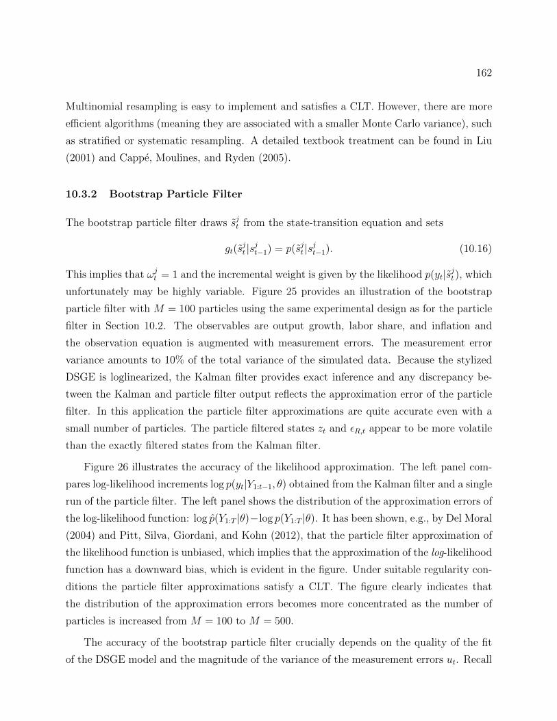
162

Multinomial resampling is easy to implement and satisfies a CLT. However, there are more

efficient algorithms (meaning they are associated with a smaller Monte Carlo variance), such

as stratified or systematic resampling. A detailed textbook treatment can be found in Liu

(2001) and Cappe, Moulines, and Ryden (2005).

10.3.2 Bootstrap Particle Filter

The bootstrap particle filter draws sjt from the state-transition equation and sets

gt(sjt |sjt−1) = p(sjt |sjt−1). (10.16)

This implies that ωjt = 1 and the incremental weight is given by the likelihood p(yt|sjt), which

unfortunately may be highly variable. Figure 25 provides an illustration of the bootstrap

particle filter with M = 100 particles using the same experimental design as for the particle

filter in Section 10.2. The observables are output growth, labor share, and inflation and

the observation equation is augmented with measurement errors. The measurement error

variance amounts to 10% of the total variance of the simulated data. Because the stylized

DSGE is loglinearized, the Kalman filter provides exact inference and any discrepancy be-

tween the Kalman and particle filter output reflects the approximation error of the particle

filter. In this application the particle filter approximations are quite accurate even with a

small number of particles. The particle filtered states zt and εR,t appear to be more volatile

than the exactly filtered states from the Kalman filter.

Figure 26 illustrates the accuracy of the likelihood approximation. The left panel com-

pares log-likelihood increments log p(yt|Y1:t−1, θ) obtained from the Kalman filter and a single

run of the particle filter. The left panel shows the distribution of the approximation errors of

the log-likelihood function: log p(Y1:T |θ)−log p(Y1:T |θ). It has been shown, e.g., by Del Moral

(2004) and Pitt, Silva, Giordani, and Kohn (2012), that the particle filter approximation of

the likelihood function is unbiased, which implies that the approximation of the log-likelihood

function has a downward bias, which is evident in the figure. Under suitable regularity con-

ditions the particle filter approximations satisfy a CLT. The figure clearly indicates that

the distribution of the approximation errors becomes more concentrated as the number of

particles is increased from M = 100 to M = 500.

The accuracy of the bootstrap particle filter crucially depends on the quality of the fit

of the DSGE model and the magnitude of the variance of the measurement errors ut. Recall

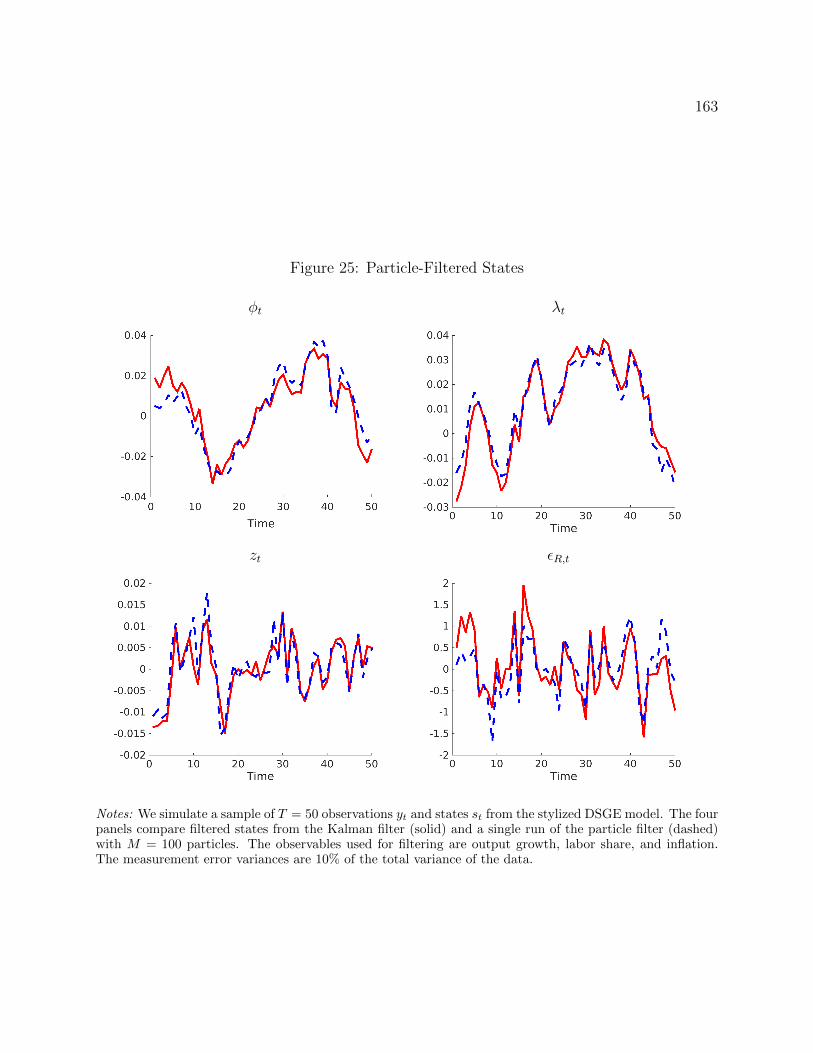
163

Figure 25: Particle-Filtered States

φt λt

zt εR,t

Notes: We simulate a sample of T = 50 observations yt and states st from the stylized DSGE model. The fourpanels compare filtered states from the Kalman filter (solid) and a single run of the particle filter (dashed)with M = 100 particles. The observables used for filtering are output growth, labor share, and inflation.The measurement error variances are 10% of the total variance of the data.

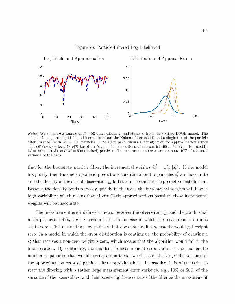
164

Figure 26: Particle-Filtered Log-Likelihood

Log-Likelihood Approximation Distribution of Approx. Errors

Notes: We simulate a sample of T = 50 observations yt and states st from the stylized DSGE model. Theleft panel compares log-likelihood increments from the Kalman filter (solid) and a single run of the particlefilter (dashed) with M = 100 particles. The right panel shows a density plot for approximation errorsof log p(Y1:T |θ) − log p(Y1:T |θ) based on Nrun = 100 repetitions of the particle filter for M = 100 (solid),M = 200 (dotted), and M = 500 (dashed) particles. The measurement error variances are 10% of the totalvariance of the data.

that for the bootstrap particle filter, the incremental weights wjt = p(yt|sjt). If the model

fits poorly, then the one-step-ahead predictions conditional on the particles sjt are inaccurate

and the density of the actual observation yt falls far in the tails of the predictive distribution.

Because the density tends to decay quickly in the tails, the incremental weights will have a

high variability, which means that Monte Carlo approximations based on these incremental

weights will be inaccurate.

The measurement error defines a metric between the observation yt and the conditional

mean prediction Ψ(st, t; θ). Consider the extreme case in which the measurement error is

set to zero. This means that any particle that does not predict yt exactly would get weight

zero. In a model in which the error distribution is continuous, the probability of drawing a

sjt that receives a non-zero weight is zero, which means that the algorithm would fail in the

first iteration. By continuity, the smaller the measurement error variance, the smaller the

number of particles that would receive a non-trivial weight, and the larger the variance of

the approximation error of particle filter approximations. In practice, it is often useful to

start the filtering with a rather large measurement error variance, e.g., 10% or 20% of the

variance of the observables, and then observing the accuracy of the filter as the measurement

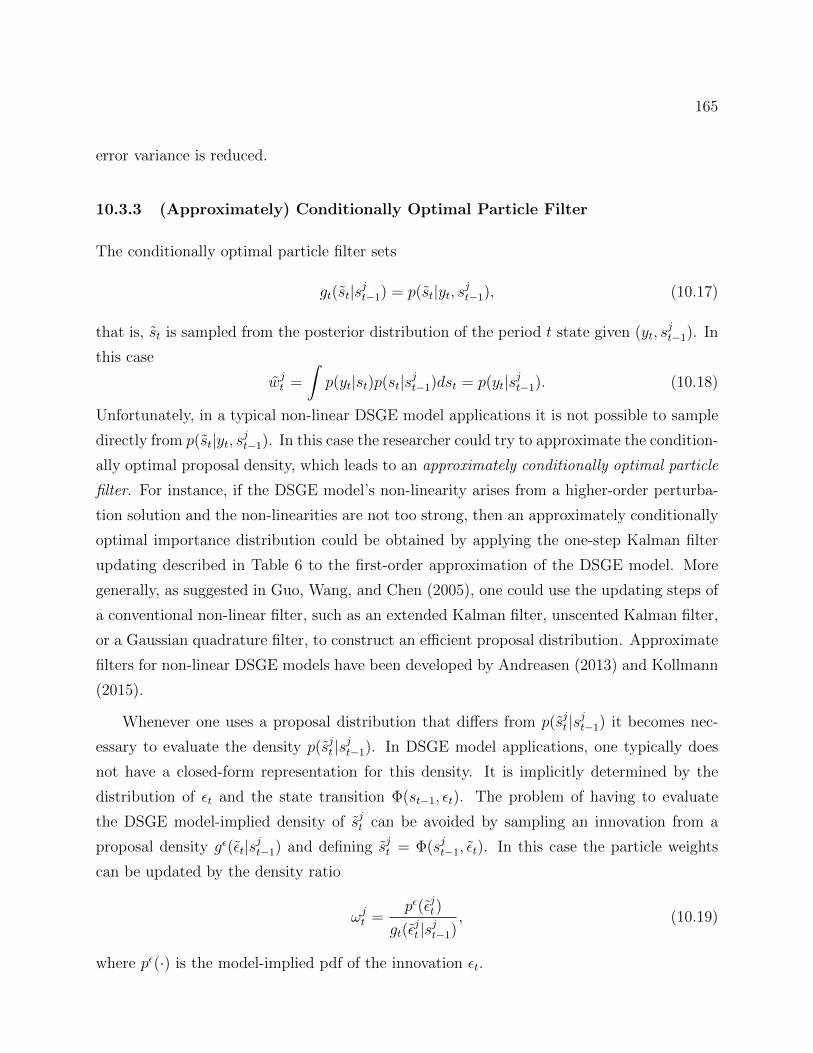
165

error variance is reduced.

10.3.3 (Approximately) Conditionally Optimal Particle Filter

The conditionally optimal particle filter sets

gt(st|sjt−1) = p(st|yt, sjt−1), (10.17)

that is, st is sampled from the posterior distribution of the period t state given (yt, sjt−1). In

this case

wjt =

∫p(yt|st)p(st|sjt−1)dst = p(yt|sjt−1). (10.18)

Unfortunately, in a typical non-linear DSGE model applications it is not possible to sample

directly from p(st|yt, sjt−1). In this case the researcher could try to approximate the condition-

ally optimal proposal density, which leads to an approximately conditionally optimal particle

filter. For instance, if the DSGE model’s non-linearity arises from a higher-order perturba-

tion solution and the non-linearities are not too strong, then an approximately conditionally

optimal importance distribution could be obtained by applying the one-step Kalman filter

updating described in Table 6 to the first-order approximation of the DSGE model. More

generally, as suggested in Guo, Wang, and Chen (2005), one could use the updating steps of

a conventional non-linear filter, such as an extended Kalman filter, unscented Kalman filter,

or a Gaussian quadrature filter, to construct an efficient proposal distribution. Approximate

filters for non-linear DSGE models have been developed by Andreasen (2013) and Kollmann

(2015).

Whenever one uses a proposal distribution that differs from p(sjt |sjt−1) it becomes nec-

essary to evaluate the density p(sjt |sjt−1). In DSGE model applications, one typically does

not have a closed-form representation for this density. It is implicitly determined by the

distribution of εt and the state transition Φ(st−1, εt). The problem of having to evaluate

the DSGE model-implied density of sjt can be avoided by sampling an innovation from a

proposal density gε(εt|sjt−1) and defining sjt = Φ(sjt−1, εt). In this case the particle weights

can be updated by the density ratio

ωjt =pε(εjt)

gt(εjt |sjt−1)

, (10.19)

where pε(·) is the model-implied pdf of the innovation εt.

166

Sometimes, DSGE models have a specific structure that may simplify the particle-filter-

based likelihood approximation. In models that are linear conditional on a subset of state

variables, e.g., volatility states or Markov-switching regimes, it is possible to use the Kalman

filter to represent the uncertainty about a subset of states. In models in which the number

of shocks εt equals the number of observables yt, it might be possible (in the absence of

measurement errors) conditional on an initial state vector s0 to directly solve for εt based

on yt and st−1, which means that it may be possible to evaluate the likelihood function

p(Y1:T |θ, s0) recursively. A more detailed discussion of these and other issues related to

particle filtering for DSGE models is provided in Herbst and Schorfheide (2015).

11 Frequentist Estimation Techniques

We will now consider four frequentist inference techniques in more detail: likelihood-based

estimation (Section 11.1), simulated method of moments estimation (Section 11.2), impulse

response function matching (Section 11.3), and GMM estimation (Section 11.4). All of

these econometric techniques, with the exception of the impulse response function matching

approach, are widely used in other areas of economics and are associated with extensive

literatures that we will not do justice to in this section. We will sketch the main idea

behind each of the econometric procedures and then focus on adjustments that have been

proposed to tailor the techniques to DSGE model applications. Each estimation method is

associated with a model evaluation procedure that essentially assesses the extent to which

the estimation objective has been achieved.

11.1 Likelihood-Based Estimation

Under the assumption that the econometric model is well specified, likelihood-based infer-

ence techniques enjoy many optimality properties. Because DSGE models deliver a joint

distribution for the observables, maximum likelihood estimation of θ is very appealing. The

maximum likelihood estimator θml was defined in (9.14). Altug (1989) and McGrattan (1994)

are early examples of papers that estimated variants of a neoclassical stochastic growth model

by maximum likelihood, whereas Leeper and Sims (1995) estimated a DSGE model meant

to be usable for monetary policy analysis.

167

Even in a loglinearized DSGE model, the DSGE model parameters θ enter the coefficients

of the state-space representation in a non-linear manner, which can be seen in Table 4. Thus,

a numerical technique is required to maximize the likelihood function. A textbook treatment

of numerical optimization routines can be found, for instance, in Judd (1998) and Nocedal

and Wright (2006). Some algorithms, e.g., Quasi-Newton methods, rely on the evaluation of

the gradient of the objective function (which requires differentiability), and other methods,

such as simulated annealing, do not. This distinction is important if the likelihood function is

evaluated with a particle filter. Without further adjustments, particle filter approximations

of the likelihood function are non-differentiable in θ even if the exact likelihood function is.

This issue and possible solutions are discussed, for instance, in Malik and Pitt (2011) and

Kantas, Doucet, Singh, Maciejowski, and Chopin (2014).

11.1.1 Textbook Analysis of the ML Estimator

Under the assumption that θ is well identified and the log-likelihood function is sufficiently

smooth with respect to θ, confidence intervals and test statistics for the DSGE model pa-

rameters can be based on a large sample approximation of the sampling distribution of the

ML estimator. A formal analysis in the context of state-space models is provided, for in-

stance, in the textbook by Cappe, Moulines, and Ryden (2005). We sketch the main steps

of the approximation, assuming that the DSGE model is correctly specified and the data are

generated by p(Y |θ0,M1). Of course, this analysis could be generalized to a setting in which

the DSGE model is misspecified and the data are generated by a reference model p(Y |M0).

In this case the resulting estimator is called quasi-maximum-likelihood estimator and the

formula for the asymptotic covariance matrix presented below would have to be adjusted. A

detailed treatment of quasi-likelihood inference is provided in White (1994).

Recall from Section 10 that the log-likelihood function can be decomposed as follows:

`T (θ|Y ) =T∑t=1

log p(yt|Y1:t−1, θ) =T∑t=1

log

∫p(yt|st, θ)p(st|Y1:t−1)dst. (11.1)

Owing to the time-dependent conditioning information Y1:t−1 the summands are not station-

ary. However, under the assumption that the sequence st, yt is stationary if initialized in

the infinite past, one can approximate the log-likelihood function by

`sT (θ|Y ) =T∑t=1

log

∫p(yt|st, θ)p(st|Y−∞:t−1)dst, (11.2)

168

and show that the discrepancy∣∣`T (θ|Y )− `sT (θ|Y )

∣∣ becomes negligible as T −→∞. The ML

estimator is consistent if T−1`sT (θ|Y )a.s.−→ `s(θ) uniformly almost surely (a.s.), where `s(θ) is

deterministic and maximized at the “true” θ0. The consistency can be stated as

θmla.s.−→ θ0. (11.3)

Frequentist asymptotics rely on a second-order approximation of the log-likelihood func-

tion. Define the score (vector of first derivatives) ∇θ`sT (θ|Y ) and the matrix of second

derivatives (Hessian, multiplied by minus one) −∇2θ`sT (θ|Y ) and let

`sT (θ|Y ) = `sT (θ0|Y ) + T−1/2∇θ`sT (θ0|Y )

√T (θ − θ0)

+1

2

√T (θ − θ0)′

[∇2θ`sT (θ0|Y )

]√T (θ − θ0) + small

If the maximum is attained in the interior of the parameter space Θ, the first-order conditions

can be approximated by

√T (θml − θ0) =

[−∇2

θ`sT (θ0|Y )

]−1T−1/2∇θ`

sT (θ0|Y ) + small. (11.4)

Under suitable regularity conditions, the score process satisfies a CLT:

T−1/2∇θ`T (θ|Y ) =⇒ N(0, I(θ0)), (11.5)

where I(θ0) is the Fisher information matrix.43 As long as the likelihood function is correctly

specified, the term ‖ − ∇2θ`T (θ|Y ) − I(θ0)‖ converges to zero uniformly in a neighborhood

around θ0, which is a manifestation of the so-called information matrix equality. This leads

to the following result √T (θml − θ0) =⇒ N

(0, I−1(θ0)

). (11.6)

Thus, standard error estimates for t-tests and confidence intervals for elements of the parame-

ter vector θ can be obtained from the diagonal elements of the inverse Hessian [−∇2θ`T (θ|Y )]−1

of the log-likelihood function evaluated at the ML estimator.44 Moreover, the maximized

likelihood function can be used to construct textbook Wald, Lagrange-multiplier, and likeli-

hood ratio statistics. Model selection could be based on a penalized likelihood function such

as the Schwarz (1978) information criterion.

43The formal definition of the information matrix for this model is delicate and therefore omitted.44Owing to the Information Matrix Equality, the standard error estimates can also be obtained from the

outer product of the score:∑Tt=1

(∇θ log p(yt|Y1:t−1, θ)

)(∇θ log p(yt|Y1:t−1, θ)

)′.

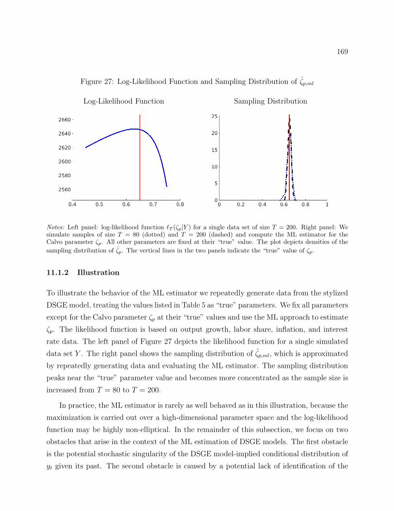
169

Figure 27: Log-Likelihood Function and Sampling Distribution of ζp,ml

Log-Likelihood Function Sampling Distribution

Notes: Left panel: log-likelihood function `T (ζp|Y ) for a single data set of size T = 200. Right panel: Wesimulate samples of size T = 80 (dotted) and T = 200 (dashed) and compute the ML estimator for theCalvo parameter ζp. All other parameters are fixed at their “true” value. The plot depicts densities of the

sampling distribution of ζp. The vertical lines in the two panels indicate the “true” value of ζp.

11.1.2 Illustration

To illustrate the behavior of the ML estimator we repeatedly generate data from the stylized

DSGE model, treating the values listed in Table 5 as “true” parameters. We fix all parameters

except for the Calvo parameter ζp at their “true” values and use the ML approach to estimate

ζp. The likelihood function is based on output growth, labor share, inflation, and interest

rate data. The left panel of Figure 27 depicts the likelihood function for a single simulated

data set Y . The right panel shows the sampling distribution of ζp,ml, which is approximated

by repeatedly generating data and evaluating the ML estimator. The sampling distribution

peaks near the “true” parameter value and becomes more concentrated as the sample size is

increased from T = 80 to T = 200.

In practice, the ML estimator is rarely as well behaved as in this illustration, because the

maximization is carried out over a high-dimensional parameter space and the log-likelihood

function may be highly non-elliptical. In the remainder of this subsection, we focus on two

obstacles that arise in the context of the ML estimation of DSGE models. The first obstacle

is the potential stochastic singularity of the DSGE model-implied conditional distribution of

yt given its past. The second obstacle is caused by a potential lack of identification of the

170

DSGE model parameters.

11.1.3 Stochastic Singularity

Imagine removing all shocks except for the technology shock from the stylized DSGE model,

while maintaining that yt comprises output growth, the labor share, inflation, and the interest

rate. In this case, we have one exogenous shock and four observables, which implies, among

other things, that the DSGE model places probability one on the event that

β logRt − log πt = β log(π∗γ/β)− log π∗.

Because in the actual data β logRt − log πt is time varying, the likelihood function is equal

to zero and not usable for inference. The literature has adopted two types of approaches

to address the singularity, which we refer to as the “measurement error” approach and the

“more structural shocks” approach.

Under the measurement error approach (8.25) is augmented by a measurement error

process ut, which in general may be serially correlated. The term “measurement error” is

a bit of a misnomer. It tries to blame the discrepancy between the model and the data

on the accuracy of the latter rather than the quality of the former. In a typical DSGE

model application, the blame should probably be shared by both. A key feature of the

“measurement error” approach is that the agents in the model do not account for the presence

of ut when making their decisions. The “measurement error” approach has been particularly

popular in the real business cycle literature – it was used, for instance, in Altug (1989). The

real business cycle literature tried to explain business cycle fluctuations based on a small

number of structural shocks, in particular, technology shocks.

The “more structural shocks” approach augments the DSGE model with additional struc-

tural shocks until the number of shocks is equal to or exceeds the desired number of observ-

ables stacked in the vector yt. For instance, if we add the three remaining shock processes

φt, λt, εR,t back into the prototypical DSGE model, then a stochastic singularity is no longer

an obstacle for the evaluation of the likelihood function. Of course, at a deeper level, the

stochastic singularity problem never vanishes, as we could also increase the dimension of

the vector yt. Because the policy functions in the solution of the DSGE model express the

control variables as functions of the state variables, the set of potential observables yt in any

171

DSGE model exceeds the number of shocks (which are exogenous state variables from the

perspective of the underlying agents’ optimization problems). Most of the literature that

estimates loglinearized DSGE models uses empirical specifications in which the number of

exogenous shocks is at least as large as the number of observables. Examples are Schorfheide

(2000), Rabanal and Rubio-Ramırez (2005), and Smets and Wouters (2007).

The converse of the “more structural shocks” approach would be a “fewer observables”

approach, i.e., one restricts the number of observables used in the construction of the likeli-

hood function to the number of exogenous shocks included in the model. This raises the ques-

tion of which observables to include in the likelihood function, which is discussed in Guerron-

Quintana (2010) and Canova, Ferroni, and Matthes (2014). Qu (2015) proposes to use a

composite likelihood to estimate singular DSGE models. A composite likelihood function is

obtained by partitioning the vector of observables yt into subsets, e.g., y′t = [y′1,t, y′2,t, y

′3,t] for

which the likelihood function is non-singular, e.g., “composite likelihood” and then use the

product of marginals p(Y1,1:T |θ)p(Y2,1:T |θ)p(Y3,1:T |θ) as the estimation objective function.

11.1.4 Dealing with Lack of Identification

In many applications it is quite difficult to maximize the likelihood function. This difficulty

is in part caused by the presence of local extrema and/or weak curvature in some directions

of the parameter space and may be a manifestation of identification problems. One potential

remedy that has been widely used in practice is to fix a subset of the parameters at plausible

values, where “plausible” means consistent with some empirical observations that are not

part of the estimation sample Y . Conditional on the fixed parameters, the likelihood function

for the remaining parameters may have a more elliptical shape and therefore may be easier

to maximize. Of course, such an approach ignores the uncertainty with respect to those

parameters that are being fixed. Moreover, if they are fixed at the “wrong” parameter

values, inference about the remaining parameters will be distorted.

Building on the broader literature on identification-robust econometric inference, the

recent literature has developed inference methods that remain valid even if some parameters

of the DSGE model are only weakly or not at all identified. Guerron-Quintana, Inoue,

and Kilian (2013) propose a method that relies on likelihood-based estimates of the system

matrices of the state-space representation Ψ0, Ψ1, Φ1 and Φε. In view of the identification

problems associated with the Ψ and Φ matrices discussed in Section 9.1, their approach

172

requires a re-parameterization of the state-space matrices in terms of an identifiable reduced-

form parameter vector φ = f(θ) that, according to the DSGE model, is a function of θ. In

the context of our stylized DSGE model, such a reparameterization could be obtained based

on the information in Table 4.

Let Mφ1 denote the state-space representation of the DSGE model in terms of φ and let φ

be the ML estimator of φ. The hypothesis H0 : θ = θ0 can be translated into the hypothesis

φ = f(θ0) and the corresponding likelihood ratio statistic takes the form

LR(Y |θ0) = 2[

log p(Y |φ,Mφ1 )− log p(Y |f(θ0),Mφ

1 )]

=⇒ χ2

dim(φ). (11.7)

The degrees of freedom of the χ2 limit distribution depend on the dimension of φ (instead

of θ), which means that it is important to reduce the dimension of φ as much as possible

by using a minimal state-variable representation of the DSGE model solution and to remove

elements from the Ψ and Φ matrices that are zero for all values of θ. The likelihood ratio

statistic can be inverted to generate a 1− α joint confidence set for the vector θ:

CSθ(Y ) =θ∣∣ LR(Y |θ) ≤ χ2

crit

, (11.8)

where χ2crit is the 1 − α quantile of the χ2

dim(φ)distribution. Sub-vector inference can be

implemented by projecting the joint confidence set on the desired subspace. The inversion

of test statistics is computationally tedious because the test statistic has to be evaluated for

a wide range of θ values. However, it does not require the maximization of the likelihood

function. Guerron-Quintana, Inoue, and Kilian (2013) show how the computation of the

confidence interval can be implemented based on the output from a Bayesian estimation of

the DSGE model.

Andrews and Mikusheva (2015) propose an identification-robust Lagrange multiplier

test. The test statistic is based on the score process and its quadratic variation

sT,t(θ) = ∇θ`(θ|Y1:t)−∇θ`(θ|Y1:t−1), JT (θ) =T∑t=1

sT,t(θ)s′T,t(θ)

and is defined as

LM(θ|Y ) = ∇′θ`T (θ0|Y )[JT (θ0)]−1∇θ`T (θ0|Y ) =⇒ χ2

dim(θ0). (11.9)

Note that the degrees of freedom of the χ2 limit distribution now depend on the dimension

of the parameter vector θ instead of the vector of identifiable reduced-form coefficients. A

173

condidence set for θ can be obtained by replacing the LR statistic in (11.8) with the LM

statistic. Andrews and Mikusheva (2015) also consider sub-vector inference based on a

profile likelihood function that concentrates out a sub-vector of well-identified DSGE model

parameters. A frequency domain version of the LM test based on the Whittle likelihood

function is provided by Qu (2014). Both Andrews and Mikusheva (2015) and Qu (2014)

provide detailed Monte Carlo studies to assess the performance of the proposed identification-

robust tests.

11.2 (Simulated) Minimum Distance Estimation

Minimum distance (MD) estimation is based on the idea of minimizing the discrepancy

between sample moments of the data, which we denoted by mT (Y ), and model-implied

moments, which we denoted by E[mT (Y )|θ,M1]. The MD estimator θmd was defined in

(9.15) and (9.16). Examples of the sample statistics mT (Y ) are the sample autocovariances

Γyy(h) or estimates of the parameters of an approximating model, e.g., the VAR(p) in (8.60)

as in Smith (1993). If mT (Y ) consists of parameter estimates of a reference model, then

the moment-based estimation is also called indirect inference; see Gourieroux, Monfort,

and Renault (1993). In some cases it is possible to calculate the model-implied moments

analytically. For instance, suppose that mT (Y ) = 1T

∑yty′t−1, then we can derive

E[mT (Y )|θ,M1] =1

T

∑E[yty

′t−1|θ,M1] = E[y2y

′1|θ,M1] (11.10)

from the state-space representation of a linearized DSGE model. Explict formulae for mo-

ments of pruned models solved with perturbation methods are provided by Andreasen,

Fernandez-Villaverde, and Rubio-Ramırez (2013) (recall Section 4.4). Alternatively, sup-

pose that mT (Y ) corresponds to the OLS estimates of a VAR(1). In this case, even for a

linear DSGE model, it is not feasible to compute

E[mT (Y )] = E

( 1

T

T∑t=1

yt−1y′t−1

)−1

1

T

T∑t=1

yt−1y′t

∣∣∣∣θ,M1

. (11.11)

The model-implied expectation of the OLS estimator has to be approximated, for instance,

by a population regression:

E[mT (Y )] =(E[yt−1y

′t−1|θ,M1]

)−1 E[yt−1y′t|θ,M1], (11.12)

174

or the model-implied moment function has to be replaced by a simulation approximation,

which will be discussed in more detail below.

11.2.1 Textbook Analysis

We proceed by sketching the asymptotic approximation of the frequentist sampling distri-

bution of the MD estimator. Define the discrepancy

GT (θ|Y ) = mT (Y )− E[mT (Y )|θ,M1], (11.13)

such that the criterion function of the MD estimator in (9.15) can be written as

QT (θ|Y ) =∥∥GT (θ|Y )

∥∥WT. (11.14)

Suppose that there is a unique θ0 with the property that45

mT (Y )− E[mT (Y )|θ0,M1]a.s.−→ 0 (11.15)

and that the sample criterion function QT (θ|Y ) converges uniformly almost surely to a limit

criterion function Q(θ), then the MD estimator is consistent in the sense that θmda.s.−→ θ0.

The analysis of the MD estimator closely mirrors the analysis of the ML estimator,

because both types of estimators are defined as the extremum of an objective function.

The sampling distribution of θmd can be derived from a second-order approximation of the

criterion function QT (θ|Y ) around θ0:

TQT (θ|Y ) =√T∇θQT (θ0|Y )

√T (θ − θ0)′ (11.16)

+1

2

√T (θ − θ0)′

[1

T∇2θQT (θ0|Y )

]√T (θ − θ0) + small.

If the minimum of QT (θ|Y ) is obtained in the interior, then

√T (θmd − θ0) =

[− 1

T∇2θQT (θ0|Y )

]−1√T∇θQT (θ0|Y ) + small. (11.17)

Using (11.13), the “score” process can be expressed as

√T∇θQT (θ0|Y ) =

(∇θGT (θ0|Y )

)WT

√TGT (θ0|Y ) (11.18)

45In some DSGE models a subset of the series included in yt is non-stationary. Thus, moments are only

well-defined after a stationarity-inducing transformation has been applied. This problem is analyzed in

Gorodnichenko and Ng (2010).

175

and its distribution depends on the distribution of

√TGT (θ0|Y ) =

√T(mT (Y )− E[mT (Y )|θ0,M1]

)(11.19)

+√T(E[mT (Y )|θ0,M1]− E[mT (Y )|θ0,M1]

)= I + II,

say. Term I captures the variability of the deviations of the sample moment mT (Y ) from

its expected value E[mT (Y )|θ0,M1] and term II captures the error due to approximating

E[mT (Y )|θ0,M1] by E[mT (Y )|θ0,M1]. Under suitable regularity conditions

√TGT (θ0|Y ) =⇒ N

(0,Ω

). (11.20)

and √T(θmd − θ0) =⇒ N

(0, (DWD′)−1DWΩWD′(DWD′)−1,

)(11.21)

where W is the limit of the sequence of weight matrices WT and the matrix D is defined as

the probability limit of ∇θGT (θ0|Y ). To construct tests and confidence sets based on the

limit distribution, the matrices D and Ω have to be replaced by consistent estimates. We

will discuss the structure of Ω in more detail below.

If the number of moment conditions exceeds the number of parameters, then the model

specification can be tested based on the overidentifying moment conditions. If WT = [ΩT ]−1,

where ΩT is a consistent estimator of Ω, then

TQT (θmd|Y ) =⇒ χ2df , (11.22)

where the degrees of freedom df equal the number of overidentifying moment conditions.

The sample objective function can also be used to construct hypothesis tests for θ. Suppose

that the null hypothesis is θ = θ0. A quasi-likelihood ratio test is based on T (QT (θ0|Y ) −QT (θmd|Y ); a quasi-Lagrange-multiplier test is based on a properly standardized quadratic

form of√T∇θQT (θ0|Y ); and a Wald test is based on a properly standardized quadratic

form of√T (θmd − θ0). Any of these test statistics can be inverted to construct a confidence

set. Moreover, if the parameters suffer from identification problems, then the approach of

Andrews and Mikusheva (2015) can be used to conduct identification-robust inference based

on the quasi-Lagrange-multiplier test.

176

11.2.2 Approximating Model-Implied Moments

In many instances the model-implied moments E[mT (Y )|θ,M1] are approximated by an

estimate E[mT (Y )|θ,M1]. This approximation affects the distribution of θmd through term II

in (11.19). Consider the earlier example in (11.11) and (11.12) in which mT (Y ) corresponds

to the OLS estimates of a VAR(1). Because the OLS estimator has a bias that vanishes at

rate 1/T , we can deduce that term II converges to zero and does not affect the asymptotic

covariance matrix Ω.

The more interesting case is the one in which E[mT (Y )|θ,M1] is based on the simulation of

the DSGE model. The asymptotic theory for simulation-based extremum estimators has been

developed in Pakes and Pollard (1989). Lee and Ingram (1991) and Smith (1993) are the first

papers that use simulated method of moments to estimate DSGE models. For concreteness,

suppose that mT (Y ) corresponds to the first-order (uncentered) sample autocovariances.

We previously showed that, provided the yt’s are stationary, E[mT (Y )|θ,M1] is given by the

DSGE model population autocovariance matrix E[y2y′1|θ,M1], which can be approximated

by simulating a sample of length λT of artificial observations Y ∗ from the DSGE model

M1 conditional on θ. Based on these simulated observations one can compute the sample

autocovariances mλT (Y ∗(θ,M1)). In this case term II is given by

II =1√λ

√λT

(1

λT

λT∑t=1

y∗t y∗t−1 − E[y2y

′1|θ0,M1]

)(11.23)

and satisfies a CLT. Because the simulated data are independent of the actual data, terms

I and II in (11.19) are independent and we can write

Ω = V∞[I] + V∞[II], (11.24)

where

V∞[II] =1

λ

(lim

T−→∞TV [mT (Y ∗(θ0,M1))]

)(11.25)

and can be derived from the DSGE model. The larger λ, the more accurate the simulation

approximation and the contribution of V∞[II] to the overall covariance matrix Ω.

We generated the simulation approximation by simulating one long sample of observa-

tions from the DSGE model. Alternatively, we could have simulated λ samples Y i, i = 1, λ

of size T . It turns out that for the approximation, say, of E[y2y′1|θ,M1], it does not matter

177

because mT (Y ∗(θ,M1)) is an unbiased estimator of E[y2y′1|θ,M1]. However, if mT (Y ) is de-

fined as the OLS estimator of a VAR(1), then the small-sample bias of the OLS estimator

generates an O(T−1) wedge between(λT∑t=1

y∗t−1y∗′t−1

)−1 λT∑t=1

y∗t−1y∗′t−1 and E

( T∑t=1

yt−1y′t−1

)−1 T∑t=1

yt−1y′t−1

∣∣∣∣θ,M1

.For large values of λ, this wedge can be reduced by using

E[mT (Y )|θ,M1] =1

λ

λ∑i=1

(T∑t=1

yit−1yi′

t−1

)−1 T∑t=1

yit−1yi′

t−1

instead. Averaging OLS estimators from model-generated data reproduces the O(T−1) bias

of the OLS estimator captured by E[mT (Y )|θ0,M1] and can lead to a final sample bias

reduction in term II, which improves the small sample performance of θmd.46

When implementing the simulation approximation of the moments, it is important to fix

the random seed when generating the sample Y ∗ such that for each parameter value of θ the

same sequence of random variables is used in computing Y ∗(θ,M1). This ensures that the

sample objective function QT (θ|Y ) remains sufficiently smooth with respect to θ to render

the second-order approximation of the objective function valid.

11.2.3 Misspecification

Under the assumption that the DSGE model is correctly specified, the MD estimator has a

well-defined almost-sure limit θ0 and the asymptotic variance V∞[I] of term I in (11.19) is

given by the model-implied variance

V∞[I] =(

limT−→∞

TV [mT (Y ∗(θ0,M1))]), (11.26)

which up to the factor of 1/λ is identical to the contribution V∞[II] of the simulation ap-

proximation of the moments to the overall asymptotic variance Ω; see (11.25). Under the

assumption of correct specification, it is optimal to choose the weight matrix W based on

the accuracy with which the elements of the moment vector mT (Y ) measure the population

46See Gourieroux, Phillips, and Yu (2010) for a formal analysis in the context of a dynamic panel data

model.

178

analog E[mT (Y )|θ0,M1]. If the number of moment conditions exceeds the number of param-

eters, it is optimal (in the sense of minimizing the sampling variance of θmd) to place more

weight on matching moments that are accurately measured in the data, by setting W = Ω−1.

In finite sample, one can construct WT from a consistent estimator of Ω−1.

If the DSGE model is regarded as misspecified, then the sampling distribution of the

MD estimator has to be derived under the distribution of a reference model p(Y |M0). In

this case we can define

θ0(Q) = limT−→∞

argminθ∥∥E[mT (Y )|M0]− E[m|θ,M1]

∣∣W

(11.27)

and, under suitable regularity, the estimator θmd will converge to the pseudo-optimal value

θ0. Note that θ0 is a function of the moments mT (Y ) that are being matched and the weight

matrix W (indicated by the Q argument). Both m and W are chosen by the researcher based

on the particular application. The vector m should correspond to a set of moments that are

deemed to be informative about the desired parameterization of the DSGE model and reflect

the ultimate purpose of the estimated DSGE model. The weight matrix W should reflect

beliefs about the informativeness of certain sample moments with respect to the desired

parameterization of the DSGE model.

To provide an example, consider the case of a DSGE model with stochastic singularity

that attributes all business cycle fluctuations to technology shocks. To the extent that the

observed data are not consistent with this singularity, the model is misspecified. A moment-

based estimation of the model will ultimately lead to inflated estimates of the standard

deviation of the technology shock innovation, because this shock alone has to generate the

observed variability in, say, output growth, the labor share, and other variables. The extent

to which the estimated shock variance is upwardly biased depends on exactly which moments

the estimator is trying to match. If one of the priorities of the estimation exercise is to match

the unconditional variance of output growth, then the weight matrix W should assign a large

weight to this moment, even if it is imprecisely measured by its sample analog in the data.

The asymptotic variance V∞[I] of term I in (11.19) is now determined by the variance

of the sample moments implied by the reference model M0:

V∞[I] =(

limT−→∞

TV[mT (Y )|M0]). (11.28)

Suppose that mT (Y ) = 1T

∑Tt=1 yty

′t−1, which under suitable regularity conditions converges

to the population autocovariance matrix E[y1y′0|M0] under the reference model M0. If the

179

reference model is a linear process, then the asymptotic theory developed in Phillips and

Solo (1992) can be used to determine the limit covariance matrix V∞[I]. An estimate of

V∞[I] can be obtained with a heteroskedasticity and autocorrelation consistent (HAC) co-

variance matrix estimator that accounts for the serial correlation in the matrix-valued se-

quence yty′t−1Tt=1. An extension of indirect inference in which mT (Y ) comprises estimates

of an approximating model to the case of misspecified DSGE models is provided in Dridi,

Guay, and Renault (2007).

11.2.4 Illustration

Detailed studies of the small-sample properties of MD estimators for DSGE models can be

found in Ruge-Murcia (2007) and Ruge-Murcia (2012). To illustrate the behavior of the MD

estimator we repeatedly generate data from the stylized DSGE model, treating the values

listed in Table 5 as “true” parameters. We fix all parameters except for the Calvo parameter

ζp at their “true” values and use two versions of the MD procedure to estimate ζp. The

vector of moment conditions mT (Y ) is defined as follows. Let yt = [log(Xt/Xt−1), πt]′ and

consider a VAR(2) in output growth and inflation:

yt = Φ1yt−1 + Φ2yt−2 + Φ0 + ut. (11.29)

Let mT (Y ) = Φ be the OLS estimate of [Φ1,Φ2,Φ0]′.

The results in the left panel of Figure 28 are obtained by a simulation approximation

of the model-implied expected value of mT (Y ). We simulate N = 100 trajectories of length

T + T0 and discarding the first T0 observations. Let Y(i)

1:T (θ) be the i-th simulated trajectory

and define

E[mT (Y )|θ,M1] ≈ 1

N

N∑i=1

mT (Y (i)(θ)), (11.30)

which can be used to evaluate the objective function (11.14). For the illustration we use

the optimal weight matrix WT = Σ−1 ⊗ X ′X, where X is the matrix of regressors for the

VAR(2) and Σ an estimate of the covariance matrix of the VAR innovations. Because we are

estimating a single parameter, we compute the estimator θmd by grid search. It is important

to use the same sequence of random numbers for each value of θ ∈ T to compute the

simulation approximation E[mT (Y )|θ,M1]. The results in the right panel of Figure 28 are

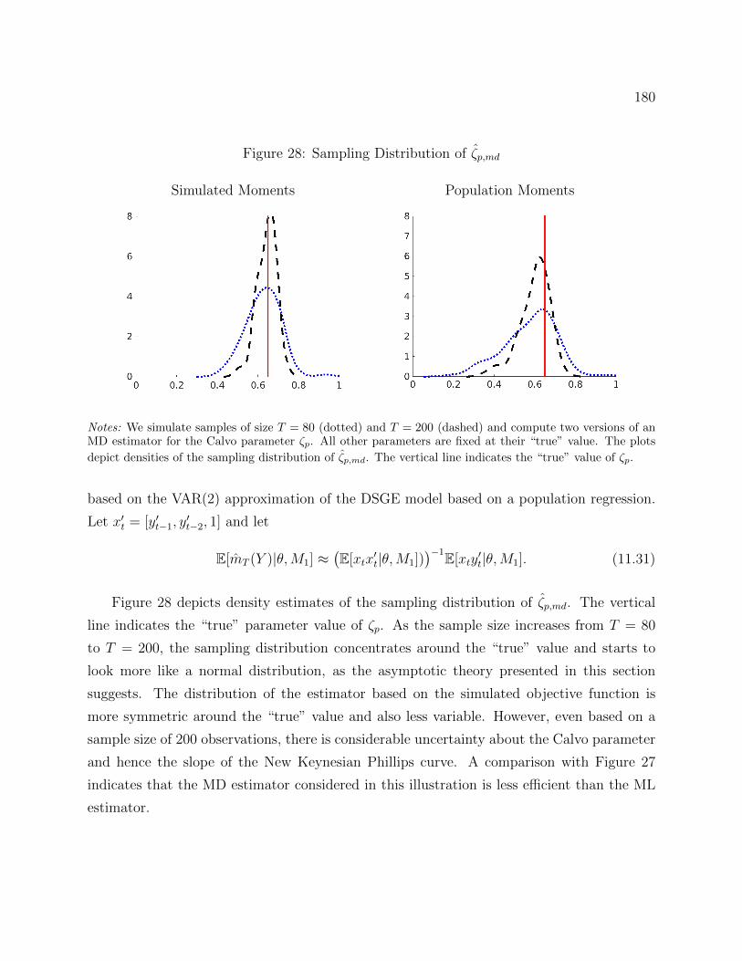
180

Figure 28: Sampling Distribution of ζp,md

Simulated Moments Population Moments

Notes: We simulate samples of size T = 80 (dotted) and T = 200 (dashed) and compute two versions of anMD estimator for the Calvo parameter ζp. All other parameters are fixed at their “true” value. The plots

depict densities of the sampling distribution of ζp,md. The vertical line indicates the “true” value of ζp.

based on the VAR(2) approximation of the DSGE model based on a population regression.

Let x′t = [y′t−1, y′t−2, 1] and let

E[mT (Y )|θ,M1] ≈(E[xtx

′t|θ,M1])

)−1E[xty′t|θ,M1]. (11.31)

Figure 28 depicts density estimates of the sampling distribution of ζp,md. The vertical

line indicates the “true” parameter value of ζp. As the sample size increases from T = 80

to T = 200, the sampling distribution concentrates around the “true” value and starts to

look more like a normal distribution, as the asymptotic theory presented in this section

suggests. The distribution of the estimator based on the simulated objective function is

more symmetric around the “true” value and also less variable. However, even based on a

sample size of 200 observations, there is considerable uncertainty about the Calvo parameter

and hence the slope of the New Keynesian Phillips curve. A comparison with Figure 27

indicates that the MD estimator considered in this illustration is less efficient than the ML

estimator.

181

11.2.5 Laplace Type Estimators

In DSGE model applications the estimation objective function QT (θ|Y ) is often difficult to

optimize. Chernozhukov and Hong (2003) proposed computing a mean of a quasi-posterior

density instead of computing an extremum estimator. The resulting estimator is called a

Laplace-type (LT) estimator and defined as follows (provided the integral in the denominator

is well defined):

θLT =exp

−1

2QT (θ|Y )

∫exp

−1

2QT (θ|Y )

dθ. (11.32)

This estimator can be evaluated using the Metropolis-Hastings algorithm discussed in Sec-

tion 12.2 or the sequential Monte Carlo algorithm presented in Section 12.3 below. The pos-

terior computations may be more accurate than the computation of an extremum. Moreover,

suppose that the objective function is multi-modal. In repeated sampling, the extremum of

the objective function may shift from one mode to the other, making the estimator appear

to be unstable. On the other hand, owing to the averaging, the LT estimator may be more

stable. Chernozhukov and Hong (2003) establish the consistency and asymptotic normality

of LT estimators, which is not surprising because the sample objective function concen-

trates around its extremum as T −→ ∞ and the discrepancy between the extremum and

the quasi-posterior mean vanishes. DSGE model applications of LT estimators are provided

in Kormilitsina and Nekipelov (2012, 2016). LT estimators can be constructed not only

from MD estimators but also from IRF matching estimators and GMM estimators discussed

below.

11.3 Impulse Response Function Matching

As discussed previously, sometimes DSGE models are misspecified because researchers have

deliberately omitted structural shocks that contribute to business cycle fluctuations. An ex-

ample of such a model is the one developed by Christiano, Eichenbaum, and Evans (2005).

The authors focus their analysis on the propagation of a single shock, namely, a monetary

policy shock. If it is clear that if the DSGE model does not contain enough structural shocks

to explain the variability in the observed data, then it is sensible to try to purge the effects

of the unspecified shocks from the data, before matching the DSGE model to the observa-

tions. This can be done by “filtering” the data through the lens of a VAR that identifies

182

the impulse responses to those shocks that are included in the DSGE model. The model pa-

rameters can then be estimated by minimizing the discrepancy between model-implied and

empirical impulse response functions. A mismatch between the two sets of impulse responses

provides valuable information about the misspecification of the propagation mechanism and

can be used to develop better-fitting DSGE models. Influential papers that estimate DSGE

models by matching impulse response functions include Rotemberg and Woodford (1997),

Christiano, Eichenbaum, and Evans (2005), and Altig, Christiano, Eichenbaum, and Linde

(2011). The casual description suggests that impulse response function matching estima-

tors are a special case of the previously discussed MD estimators (the DSGE model M1 is

misspecified and a structural VAR serves as reference model M0 under which the sampling

distribution of the estimator is derived). Unfortunately, several complications arise, which

we will discuss in the remainder of this section. Throughout, we assume that the DSGE

model has been linearized. An extension to the case of non-linear DSGE models is discussed

in Ruge-Murcia (2014).

11.3.1 Invertibility and Finite-Order VAR Approximations

The empirical impulse responses are based on a finite-order VAR, such as the one in (8.60).

However, even linearized DSGE models typically cannot be written as a finite-order VAR.

Instead, they take the form of a state-space model, which typically has a VARMA represen-

tation. In general we can distinguish the following three cases: (i) the solution of the DSGE

model can be expressed as a VAR(p). For the stylized DSGE model, this is the case if yt is

composed of four observables: output growth, the labor share, inflation, and interest rates.

(ii) The moving average polynomial of the VARMA representation of the DSGE model is

invertible. In this case the DSGE model can be expressed as an infinite-order VAR driven by

the structural shock innovations εt. (iii) The moving average polynomial of the VARMA rep-

resentation of the DSGE model is not invertible. In this case the innovation of the VAR(∞)

approximation do not correspond to the structural innovations εt. Only in case (i) can one

expect a direct match between the empirical IRFs and the DSGE model IRFs. Cases (ii) and

(iii) complicate econometric inference. The extent to which impulse-response-function-based

estimation and model evaluation may be misleading has been fiercely debated in Christiano,

Eichenbaum, and Vigfusson (2007) and Chari, Kehoe, and McGrattan (2008).

183

Fernandez-Villaverde, Rubio-Ramırez, Sargent, and Watson (2007) provide formal cri-

teria to determine whether a DSGE model falls under case (i), (ii), or (iii). Rather than

presenting a general analysis of this problem, we focus on a simple example. Consider the

following two MA processes that represent the DSGE models in this example:

M1 : yt = εt + θεt−1 = (1 + θL)εt (11.33)

M2 : yt = θεt + εt−1 = (θ + L)εt,

where 0 < θ < 1, L denotes the lag operator, and εt ∼ iidN(0, 1). Models M1 and M2

are observationally equivalent, because they are associated with the same autocovariance

sequence. The root of the MA polynomial of model M1 is outside of the unit circle, which

implies that the MA polynomial is invertible and one can express yt as an AR(∞) process:

AR(∞) for M1 : yt = −∞∑j=1

(−θ)jyt−j + εt. (11.34)

It is straightforward to verify that the AR(∞) approximation reproduces the impulse re-

sponse function of M1:

∂yt∂εt

= 1,∂yt+1

∂εt= θ,

∂yt+h∂εt

= 0 for h > 1.

Thus, the estimation of an autoregressive model with many lags can reproduce the monotone

impulse response function of model M1.

The root of the MA polynomial of M2 lies inside the unit circle. While M2 could also

be expressed as an AR(∞), it would be a representation in terms of a serially uncorrelated

one-step-ahead forecast error ut that is a function of the infinite history of the εt’s: ut =

(1 + θL)−1(θ + L). As a consequence, the AR(∞) is unable to reproduce the hump-shaped

IRF of model M2. More generally, if the DSGE model is associated with a non-invertible

moving average polynomial, its impulse responses cannot be approximated by a VAR(∞)

and a direct comparison of VAR and DSGE IRFs may be misleading.

11.3.2 Practical Considerations

The objective function for the IRF matching estimator takes the same form as the criterion

function of the method of moments estimator in (11.13) and (11.14), where mT (Y ) is the

184

VAR IRF. For E[mT (Y )|θ,M1] researchers typically just use the DSGE model impulse re-

sponse, say, IRF (·|θ,M1). In view of the problems caused by non-invertible moving-average

polynomials and finite-order VAR approximations of infinite-order VAR representations, a

more prudent approach would be to replace IRF (·|θ,M1) by average impulse response func-

tions that are obtained by repeatedly simulating data from the DSGE model (given θ) and

estimating a structural VAR, as in the indirect inference approach described in Section 11.2.

Such a modification would address the concerns about IRF matching estimators raised by

Chari, Kehoe, and McGrattan (2008).

The sampling distribution of the IRF matching estimator depends on the sampling dis-

tribution of the empirical VAR impulse responses mT (Y ) under the VAR M0. An approx-

imation of the distribution of mT (Y ) could be obtained by first-order asymptotics and the

delta method as in Lutkepohl (1990) and Mittnik and Zadrozny (1993) for stationary VARs;

or as in Phillips (1998), Rossi and Pesavento (2006), and Pesavento and Rossi (2007) for

VARs with persistent components. Alternatively, one could use the bootstrap approxima-

tion proposed by Kilian (1998, 1999). If the number of impulse responses stacked in the

vector mT (Y ) exceeds the number of reduced-form VAR coefficient estimates, then the sam-

pling distribution of the IRFs becomes asymptotically singular. Guerron-Quintana, Inoue,

and Kilian (2014) use non-standard asymptotics to derive the distribution of IRFs for the

case in which there are more responses than reduced-form parameters.

Because for high-dimensional vectors mT (Y ) the joint covariance matrix may be close

to singular, researchers typically choose a diagonal weight matrix WT , where the diagonal

elements correspond to the inverse of the sampling variance for the estimated response of

variable i to shock j at horizon h. As discussed in Section 11.2, to the extent that the DSGE

model is misspecified, the choice of weight matrix affects the probability limit of the IRF

matching estimator and should reflect the researcher’s loss function.

In fact, impulse response function matching is appealing only if the researcher is con-

cerned about model misspecification. This misspecification might take two forms: First, the

propagation mechanism of the DSGE model is potentially misspecified and the goal is to

find pseudo-optimal parameter values that minimize the discrepancy between empirical and

model-implied impulse responses. Second, the propagation mechanisms for the shocks of in-

terest are believed to be correctly specified, but the model lacks sufficiently many stochastic

shocks to capture the observed variation in the data. In the second case, it is in principle

185

possible to recover the subset of “true” DSGE model parameters θ0 that affect the propaga-

tion of the structural shock for which the IRF is computed. The consistent estimation would

require that the DSGE model allow for a VAR(∞) representation in terms of the structural

shock innovations εt; that the number of lags included in the empirical VAR increase with

sample size T ; and that the VAR identification scheme correctly identify the shock of interest

if the data are generated from a version of the DSGE model that is augmented by additional

structural shocks.

11.3.3 Illustration

To illustrate the properties of the IRF matching estimator, we simulate data from the stylized

DSGE model using the parameter values given in Table 5. We assume that the econometri-

cian considers an incomplete version of the DSGE model that only includes the monetary

policy shock and omits the remaining shocks. Moreover, we assume that the econometrician

only has to estimate the degree of price stickiness captured by the Calvo parameter ζp. All

other parameters are fixed at their “true” values during the estimation.

The empirical impulse response functions stacked in the vector mT (Y ) are obtained by

estimating a VAR(p) for interest rates, output growth, and inflation:

yt =[Rt − πt/β, log(Xt/Xt−1), πt

]′. (11.35)

The first equation of this VAR represents the monetary policy rule of the DSGE model. The

interest rate is expressed in deviations from the central bank’s systematic reaction to infla-

tion. Thus, conditional on β, the monetary policy shock is identified as the orthogonalized

one-step-ahead forecast error in the first equation of the VAR. Upon impact, the response of

yt to the monetary policy shock is given by the first column of the lower-triangular Cholesky

factor of the covariance matrix Σ of the reduced-form innovations ut.

Because yt excludes the labor share, the state-space representation of the DSGE model

cannot be expressed as a finite-order VAR. However, we can construct a VAR approximation

of the DSGE model as follows. Let xt = [y′t−1, . . . , y′t−p, 1

′]′ and define the functions47

Φ∗(θ) =(E[xtx

′t|θ,M1]

)−1(E[xty′t|θ,M1]

), (11.36)

Σ∗(θ) = E[yty′t|θ,M1]− E[ytx

′t|θ,M1]

(E[xtx

′t|θ,M1]

)−1E[xty′t|θ,M1].

47For the evaluation of the moment matrices E[·|θ,M1] see Section 8.2.1.

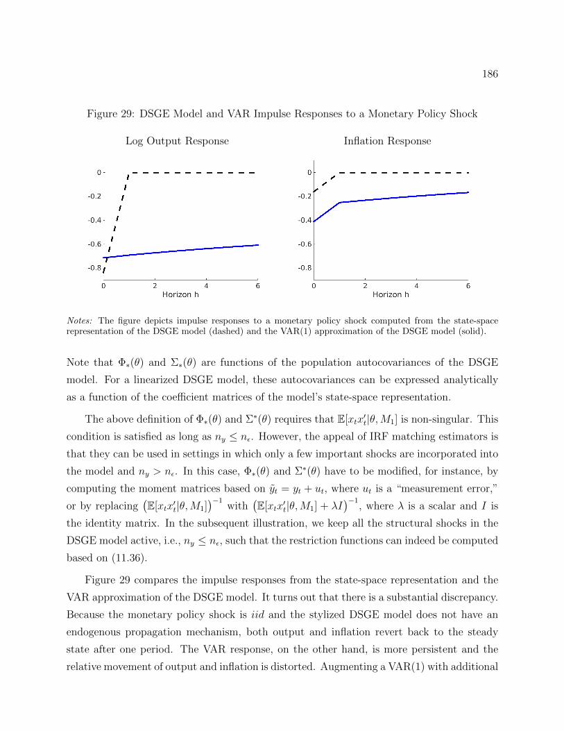
186

Figure 29: DSGE Model and VAR Impulse Responses to a Monetary Policy Shock

Log Output Response Inflation Response

Notes: The figure depicts impulse responses to a monetary policy shock computed from the state-spacerepresentation of the DSGE model (dashed) and the VAR(1) approximation of the DSGE model (solid).

Note that Φ∗(θ) and Σ∗(θ) are functions of the population autocovariances of the DSGE

model. For a linearized DSGE model, these autocovariances can be expressed analytically

as a function of the coefficient matrices of the model’s state-space representation.

The above definition of Φ∗(θ) and Σ∗(θ) requires that E[xtx′t|θ,M1] is non-singular. This

condition is satisfied as long as ny ≤ nε. However, the appeal of IRF matching estimators is

that they can be used in settings in which only a few important shocks are incorporated into

the model and ny > nε. In this case, Φ∗(θ) and Σ∗(θ) have to be modified, for instance, by

computing the moment matrices based on yt = yt + ut, where ut is a “measurement error,”

or by replacing(E[xtx

′t|θ,M1]

)−1with

(E[xtx

′t|θ,M1] + λI

)−1, where λ is a scalar and I is

the identity matrix. In the subsequent illustration, we keep all the structural shocks in the

DSGE model active, i.e., ny ≤ nε, such that the restriction functions can indeed be computed

based on (11.36).

Figure 29 compares the impulse responses from the state-space representation and the

VAR approximation of the DSGE model. It turns out that there is a substantial discrepancy.

Because the monetary policy shock is iid and the stylized DSGE model does not have an

endogenous propagation mechanism, both output and inflation revert back to the steady

state after one period. The VAR response, on the other hand, is more persistent and the

relative movement of output and inflation is distorted. Augmenting a VAR(1) with additional

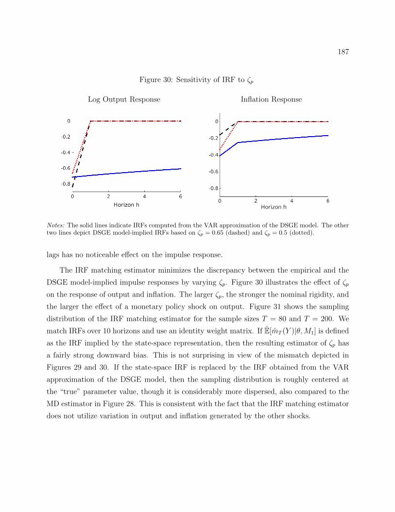
187

Figure 30: Sensitivity of IRF to ζp

Log Output Response Inflation Response

Notes: The solid lines indicate IRFs computed from the VAR approximation of the DSGE model. The othertwo lines depict DSGE model-implied IRFs based on ζp = 0.65 (dashed) and ζp = 0.5 (dotted).

lags has no noticeable effect on the impulse response.

The IRF matching estimator minimizes the discrepancy between the empirical and the

DSGE model-implied impulse responses by varying ζp. Figure 30 illustrates the effect of ζp

on the response of output and inflation. The larger ζp, the stronger the nominal rigidity, and

the larger the effect of a monetary policy shock on output. Figure 31 shows the sampling

distribution of the IRF matching estimator for the sample sizes T = 80 and T = 200. We

match IRFs over 10 horizons and use an identity weight matrix. If E[mT (Y )|θ,M1] is defined

as the IRF implied by the state-space representation, then the resulting estimator of ζp has

a fairly strong downward bias. This is not surprising in view of the mismatch depicted in

Figures 29 and 30. If the state-space IRF is replaced by the IRF obtained from the VAR

approximation of the DSGE model, then the sampling distribution is roughly centered at

the “true” parameter value, though it is considerably more dispersed, also compared to the

MD estimator in Figure 28. This is consistent with the fact that the IRF matching estimator

does not utilize variation in output and inflation generated by the other shocks.

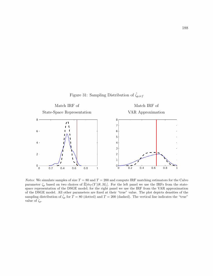
188

Figure 31: Sampling Distribution of ζp,irf

Match IRF of Match IRF of

State-Space Representation VAR Approximation

Notes: We simulate samples of size T = 80 and T = 200 and compute IRF matching estimators for the Calvoparameter ζp based on two choices of E[mT (Y )|θ,M1]. For the left panel we use the IRFs from the state-space representation of the DSGE model; for the right panel we use the IRF from the VAR approximationof the DSGE model. All other parameters are fixed at their “true” value. The plot depicts densities of the

sampling distribution of ζp for T = 80 (dotted) and T = 200 (dashed). The vertical line indicates the “true”value of ζp.

189

11.4 GMM Estimation

We showed in Section 8.2.4 that one can derive moment conditions of the form

E[g(yt−p:t|θ,M1)] = 0 (11.37)

for θ = θ0 from the DSGE model equilibrium. For instance, based on (8.53) and (8.54) we

could define

g(yt−p:t|θ,M1) =

[ (− log(Xt/Xt−1) + logRt−1 − log πt − log(1/β)

)Zt−1(

logRt − log(γ/β)− ψ log πt − (1− ψ) log π∗)Zt−1

]. (11.38)

The identifiability of θ requires that the moments be different from zero whenever θ 6= θ0. A

GMM estimator is obtained by replacing population expectations by sample averages. Let

GT (θ|Y ) =1

T

T∑t=1

g(yt−p:t|θ,M1). (11.39)

The GMM objective function is given by

QT (θ|Y ) = GT (θ|Y )′WTGT (θ|Y ) (11.40)

and looks identical to the objective function studied in Section 11.2. In turn, the analysis of

the sampling distribution of θmd carries over to the GMM estimator.

The theoretical foundations of GMM estimation were developed by Hansen (1982), who

derived the first-order asymptotics for the estimator assuming that the data are stationary

and ergodic. Christiano and Eichenbaum (1992) and Burnside, Eichenbaum, and Rebelo

(1993) use GMM to estimate the parameters of real business cycle DSGE models. These

papers use sufficiently many moment conditions to be able to estimate all the parameters

of their respective DSGE models. GMM estimation can also be applied to a subset of the

equilibrium conditions, e.g., the consumption Euler equation or the New Keynesian Phillips

curve to estimate the parameters related to these equilibrium conditions.

Unlike all the other estimators considered in this paper, the GMM estimators do not

require the researchers to solve the DSGE model. To the extent that solving the model is

computationally costly, this can considerably speed up the estimation process. Moreover,

one can select moment conditions that do not require assumptions about the law of motion of

exogenous driving processes, which robustifies the GMM estimator against misspecification of

190

the exogenous propagation mechanism. However, it is difficult to exploit moment conditions

in which some of the latent variables appear explicitly. For instance, consider the Phillips

curve relationship of the stylized DSGE model, which suggests setting

g(yt−p:t|θ,M1) =(πt−1 − βπt − κp(lsht−1)

)Zt−1. (11.41)

Note that λt−1 is omitted from the definition of g(yt−p:t|θ,M1) because it is unobserved. How-

ever, as soon as Zt is correlated with the latent variable λt the expected value of g(yt−p:t|θ,M1)

is non-zero even for θ = θ0:

E[g(yt−p:t|θ0,M1)] = −κ0E[λt−1Zt−1] 6= 0. (11.42)

To the extent that λt is serially correlated, using higher-order lags of yt as instruments does

not solve the problem.48 Recent work by Gallant, Giacomini, and Ragusa (2013) and Shin

(2014) considers extensions of GMM estimation to moment conditions with latent variables.

The recent literature on GMM estimation of DSGE models has focused on identification-

robust inference in view of the weak identification of Phillips curve and monetary policy

rule parameters. Generic identification problems in the context of monetary policy rule

estimation are highlighted in Cochrane (2011) and methods to conduct identification-robust

inference are developed in Mavroeidis (2010). Identification-robust inference for Phillips

curve parameters is discussed in Mavroeidis (2005), Kleibergen and Mavroeidis (2009), and

Mavroeidis, Plagborg-Moller, and Stock (2014). Dufour, Khalaf, and Kichian (2013) consider

identification-robust moment-based estimation of all of the equilibrium relationships of a

DSGE model.

12 Bayesian Estimation Techniques

Bayesian inference is widely used in empirical work with DSGE models. The first pa-

pers to estimate small-scale DSGE models using Bayesian methods were DeJong, Ingram,

and Whiteman (2000), Schorfheide (2000), Otrok (2001), Fernandez-Villaverde and Rubio-

Ramırez (2004), and Rabanal and Rubio-Ramırez (2005). Subsequent papers estimated

48Under the assumption that λt follows an AR(1) process, one could quasi-difference the Phillips curve,

which would replace the term λt−1Zt−1 with ελ,t−1Zt−1. If Zt−1 is composed of lagged observables dated

t− 2 and earlier, then the validity of the moment condition is restored.

191

open-economy DSGE models, e.g., Lubik and Schorfheide (2006), and larger DSGE models

tailored to the analysis of monetary policy, e.g., Smets and Wouters (2003) and Smets and

Wouters (2007). Because Bayesian analysis treats shock, parameter, and model uncertainty

symmetrically by specifying a joint distribution that is updated in view of the observations

Y , it provides a conceptually appealing framework for decision making under uncertainty.

Levin, Onatski, Williams, and Williams (2006) consider monetary policy analysis under un-

certainty based on an estimated DSGE model and the handbook chapter by Del Negro and

Schorfheide (2013) focuses on forecasting with DSGE models.

Conceptually, Bayesian inference is straightforward. A prior distribution is updated in

view of the sample information contained in the likelihood function. This leads to a posterior

distribution that summarizes the state of knowledge about the unknown parameter vector

θ. The main practical difficulty is the calculation of posterior moments and quantiles of

transformations h(·) of the parameter vector θ. The remainder of this section is organized as

follows. We provide a brief discussion of the elicitation of prior distributions in Section 12.1.

Sections 12.2 and 12.3 discuss two important algorithms to generate parameter draws from

posterior distributions: Markov chain Monte Carlo (MCMC) and sequential Monte Carlo

(SMC). Bayesian model diagnostics are reviewed in Section 12.4. Finally, we discuss the

recently emerging literature on limited-information Bayesian inference in Section 12.5. Sec-

tions 12.1 to 12.3 are based on Herbst and Schorfheide (2015), who provide a much more

detailed exposition. Section 12.4 draws from Del Negro and Schorfheide (2011).

12.1 Prior Distributions

There is some disagreement in the Bayesian literature about the role of prior information in

econometric inference. Some authors advocate “flat” prior distributions that do not distort

the shape of the likelihood function, which raises two issues: first, most prior distributions are

not invariant under parameter transformations. Suppose a scalar parameter θ ∼ U [−M,M ].

If the model is reparameterized in terms of 1/θ, the implied prior is no longer flat. Second,

if the prior density is taken to be constant on the real line, say, p(θ) = c, then the prior is no

longer proper, meaning the total prior probability mass is infinite. In turn, it is no longer

guaranteed that the posterior distribution is proper.

In many applications prior distributions are used to conduct inference in situations in

192

which the number of unknown parameters is large relative to the number of sample obser-

vations. An example is a high-dimensional VAR. If the number of variables in the VAR is n

and the number of lags is p, then each equation has at least np unknown parameters. For in-

stance, a 4-variable VAR with p = 4 lags has 16 parameters. If this model is estimated based

on quarterly post-Great Moderation and pre-Great Recession data, the data-to-parameter

ratio is approximately 6, which leads to very noisy parameter estimates. A prior distribu-

tion essentially augments the estimation sample Y by artificial observations Y ∗ such that

the model is estimated based on the combined sample (Y, Y ∗).

Prior distributions can also be used to “regularize” the likelihood function by giving the

posterior density a more elliptical shape. Finally, a prior distribution can be used to add

substantive information about model parameters not contained in the estimation sample

θ to the inference problem. Bayesian estimation of DSGE models uses prior distributions

mostly to add information contained in data sets other than Y and to smooth out the

likelihood function, down-weighing regions of the parameter space in which implications of

the structural model contradict non-sample information and the model becomes implausible.

An example would be a DSGE model with a likelihood that has a local maximum at which

the discount factor is, say, β = 0.5. Such a value of β would strongly contradict observations

of real interest rates. A prior distribution that implies that real interest rates are between 0

and 10% with high probability would squash the undesirable local maximum of the likelihood

function.

To the extent that the prior distribution is “informative” and affects the shape of the

posterior distribution, it is important that the specification of the prior distribution be

carefully documented. Del Negro and Schorfheide (2008) developed a procedure to construct

prior distributions based on information contained in pre-samples or in time series that are

not directly used for the estimation of the DSGE model. To facilitate the elicitation of a

prior distribution it is useful to distinguish three groups of parameters: steady-state-related

parameters, exogenous shock parameters, and endogenous propagation parameters.

In the context of the stylized DSGE model, the steady-state-related parameters are given

by β (real interest rate), π∗ (inflation), γ (output growth rate), and λ (labor share). A prior

for these parameters could be informed by pre-sample averages of these series. The endoge-

nous propagation parameters are ζp (Calvo probability of not being able to re-optimize price)

and ν (determines the labor supply elasticity). Micro-level information about the frequency

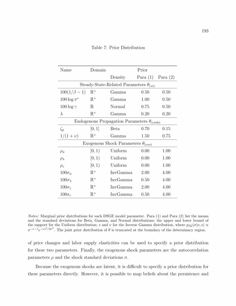
193

Table 7: Prior Distribution

Name Domain Prior

Density Para (1) Para (2)

Steady-State-Related Parameters θ(ss)

100(1/β − 1) R+ Gamma 0.50 0.50

100 log π∗ R+ Gamma 1.00 0.50

100 log γ R Normal 0.75 0.50

λ R+ Gamma 0.20 0.20

Endogenous Propagation Parameters θ(endo)

ζp [0, 1] Beta 0.70 0.15

1/(1 + ν) R+ Gamma 1.50 0.75

Exogenous Shock Parameters θ(exo)

ρφ [0, 1) Uniform 0.00 1.00

ρλ [0, 1) Uniform 0.00 1.00

ρz [0, 1) Uniform 0.00 1.00

100σφ R+ InvGamma 2.00 4.00

100σλ R+ InvGamma 0.50 4.00

100σz R+ InvGamma 2.00 4.00

100σr R+ InvGamma 0.50 4.00

Notes: Marginal prior distributions for each DSGE model parameter. Para (1) and Para (2) list the meansand the standard deviations for Beta, Gamma, and Normal distributions; the upper and lower bound ofthe support for the Uniform distribution; s and ν for the Inverse Gamma distribution, where pIG(σ|ν, s) ∝σ−ν−1e−νs

2/2σ2

. The joint prior distribution of θ is truncated at the boundary of the determinacy region.

of price changes and labor supply elasticities can be used to specify a prior distribution

for these two parameters. Finally, the exogenous shock parameters are the autocorrelation

parameters ρ and the shock standard deviations σ.

Because the exogenous shocks are latent, it is difficult to specify a prior distribution for

these parameters directly. However, it is possible to map beliefs about the persistence and

194

volatility of observables such as output growth, inflation, and interest rates into beliefs about

the exogenous shock parameters. This can be done using the formal procedure described in

Del Negro and Schorfheide (2008) or, informally, by generating draws of θ from the prior

distribution, simulating artificial observations from the DSGE model, and computing the im-

plied sample moments of the observables. If the prior predictive distribution of these sample

moments appears implausible, say, in view of sample statistics computed from a pre-sample

of actual observations, then one can adjust the prior distribution of the exogenous shock

parameters and repeat the simulation until a plausible prior is obtained. Table 7 contains

an example of a prior distribution for our stylized DSGE model. The joint distribution for

θ is typically generated as a product of marginal distributions for the elements (or some

transformations thereof) of the vector θ.49 In most applications this product of marginals is

truncated to ensure that the model has a unique equilibrium.

12.2 Metropolis-Hastings Algorithm

Direct sampling from the posterior distribution of θ is unfortunately not possible. One widely

used algorithm to generate draws from p(θ|Y ) is the Metropolis-Hastings (MH) algorithm,

which belongs to the class of MCMC algorithms. MCMC algorithms produce a sequence

of serially correlated parameter draws θi, i = 1, . . . , N with the property that the random

variables θi converge in distribution to the target posterior distribution, which we abbreviate

as

π(θ) = p(θ|Y ) =p(Y |θ)p(θ)p(Y )

(12.1)

as N −→∞. More important, under suitable regularity conditions sample averages of draws

converge to posterior expectations:

1

N −N0

N∑i=N0+1

h(θi)a.s.−→ Eπ[h(θ)]. (12.2)

Underlying this convergence result is the fact that the algorithm generates a Markov tran-

sition kernel K(θi|θi−1), characterizing the distribution of θi conditional on θi−1, with the

49In high-dimensional parameter spaces it might be desirable to replace some of the θ elements by trans-

formations, e.g., steady states, that are more plausibly assumed to be independent. This transformation

essentially generates non-zero correlations for the original DSGE model parameters. Alternatively, the

method discussed in Del Negro and Schorfheide (2008) also generates correlations between parameters.

195

invariance property ∫K(θi|θi−1)π(θi−1)dθi−1 = π(θi). (12.3)

Thus, if θi−1 is a draw from the posterior distribution, then so is θi. Of course, this invariance

property is not sufficient to guarantee the convergence of the θi draws. Chib and Greenberg

(1995) provide an excellent introduction to MH algorithms and detailed textbook treatments

can be found, for instance, in Robert and Casella (2004) and Geweke (2005).

12.2.1 The Basic MH Algorithm

The key ingredient of the MH algorithm is a proposal distribution q(ϑ|θi−1), which potentially

depends on the draw θi−1 in iteration i − 1 of the algorithm. With probability α(ϑ|θi−1)

the proposed draw is accepted and θi = ϑ. If the proposed draw is not accepted, then the

chain does not move and θi = θi−1. The acceptance probability is chosen to ensure that the

distribution of the draws converges to the target posterior distribution. The algorithm takes

the following form:

Algorithm 7 (Generic MH Algorithm). For i = 1 to N:

1. Draw ϑ from a density q(ϑ|θi−1).

2. Set θi = ϑ with probability

α(ϑ|θi−1) = min

1,

p(Y |ϑ)p(ϑ)/q(ϑ|θi−1)

p(Y |θi−1)p(θi−1))/q(θi−1|ϑ)

and θi = θi−1 otherwise.

Because p(θ|Y ) ∝ p(Y |θ)p(θ) we can replace the posterior densities in the calculation of

the acceptance probabilities α(ϑ|θi−1) with the product of the likelihood and prior, which

does not require the evaluation of the marginal data density p(Y ).

12.2.2 Random-Walk Metropolis-Hastings Algorithm

The most widely used MH algorithm for DSGE model applications is the random walk MH

(RWMH) algorithm. The basic version of this algorithm uses a normal distribution centered

at the previous θi draw as the proposal density:

ϑ|θi ∼ N(θi, c2Σ) (12.4)

196

Given the symmetric nature of the proposal distribution, the acceptance probability becomes

α = min

p(ϑ|Y )

p(θi−1|Y ), 1

.

A draw, ϑ, is accepted with probability one if the posterior at ϑ has a higher value than the

posterior at θi−1. The probability of acceptance decreases as the posterior at the candidate

value decreases relative to the current posterior.

To implement the RWMH, the user needs to specify c, and Σ. The proposal variance

controls the relative variances and correlations in the proposal distribution. The sampler

can work very poorly if q is strongly at odds with the target distribution. A good choice for

Σ seeks to incorporate information from the posterior, to potentially capture the a posteriori

correlations among parameters. Obtaining this information can be difficult. A popular

approach, used in Schorfheide (2000), is to set Σ to be the negative of the inverse Hessian at

the mode of the log posterior, θ, obtained by running a numerical optimization routine before

running MCMC. Using this as an estimate for the covariance of the posterior is attractive,

because it can be viewed as a large sample approximation to the posterior covariance matrix.

Unfortunately, in many applications, the maximization of the posterior density is tedious

and the numerical approximation of the Hessian may be inaccurate. These problems may

arise if the posterior distribution is very non-elliptical and possibly multimodal, or if the

likelihood function is replaced by a non-differentiable particle filter approximation. In both

cases, a (partially) adaptive approach may work well: First, generate a set of posterior draws

based on a reasonable initial choice for Σ, e.g. the prior covariance matrix. Second, compute

the sample covariance matrix from the first sequence of posterior draws and use it as Σ in a

second run of the RWMH algorithm. In principle, the covariance matrix Σ can be adjusted

more than once. However, Σ must be fixed eventually to guarantee the convergence of the

posterior simulator. Samplers that constantly (or automatically) adjust Σ are known as

adaptive samplers and require substantially more elaborate theoretical justifications.

12.2.3 Numerical Illustration

We generate a single sample of size T = 80 from the stylized DSGE model using the pa-

rameterization in Table 5. The DSGE model likelihood function is combined with the prior

distribution in Table 7 to form a posterior distribution. Draws from this posterior distribu-

tion are generated using the RWMH described in the previous section. The chain is initialized

197

with a draw from the prior distribution. The covariance matrix Σ is based on the negative

inverse Hessian at the mode. The scaling constant c is set equal to 0.075, which leads to an

acceptance rate for proposed draws of 0.55.

The top panels of Figure 32 depict the sequences of posterior draws of the Calvo param-

eter ζ ip and preference shock standard deviation σiφ. It is apparent from the figure that the

draws are serially correlated. The draws for the standard deviation are strongly contami-

nated by the initialization of the chain, but they eventually settle to a range of 0.8 to 1.1.

The bottom panel depicts recursive means of the form

hN |N0 =1

N −N0

N∑i=N0+1

h(θi). (12.5)

To remove the effect of the initialization of the Markov chain, it is common to drop the first

N0 draws from the computation of the posterior mean approximation. In the figure we set

N0 = 7, 500 and N = 37, 500. Both recursive means eventually settle to a limit point.

The output of the algorithm is stochastic, which implies that running the algorithm

repeatedly will generate different numerical results. Under suitable regularity conditions the

recursive means satisfy a CLT. The easiest way to obtain a measure of numerical accuracy is

to run the RWMH algorithm, say, fifty times using random starting points, and compute the

sample variance of hN |N0 across chains. Alternatively, one could compute a heteroskedasticity

and autocorrelation consistent (HAC) standard error estimate for hN |N0 based on the output

of a single chain.

Figure 33 depicts univariate prior and posterior densities, which are obtained by applying

a standard kernel density estimator to draws from the prior and posterior distribution. In

addition, one can also compute posterior credible sets based on the output of the posterior

sampler. For a univariate parameter, the shortest credible set is given by the highest-

posterior-density (HPD) set defined as

CSHPD(Y ) =θ∣∣p(θ|Y ) ≥ κα

, (12.6)

where κα is chosen to ensure that the credible set has the desired posterior coverage proba-

bility.

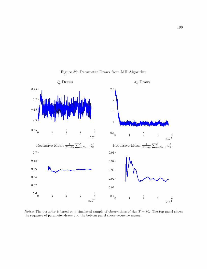
198

Figure 32: Parameter Draws from MH Algorithm

ζ ip Draws σiφ Draws

Recursive Mean 1N−N0

∑Ni=N0+1 ζ

ip Recursive Mean 1

N−N0

∑Ni=N0+1 σ

iφ

Notes: The posterior is based on a simulated sample of observations of size T = 80. The top panel showsthe sequence of parameter draws and the bottom panel shows recursive means.

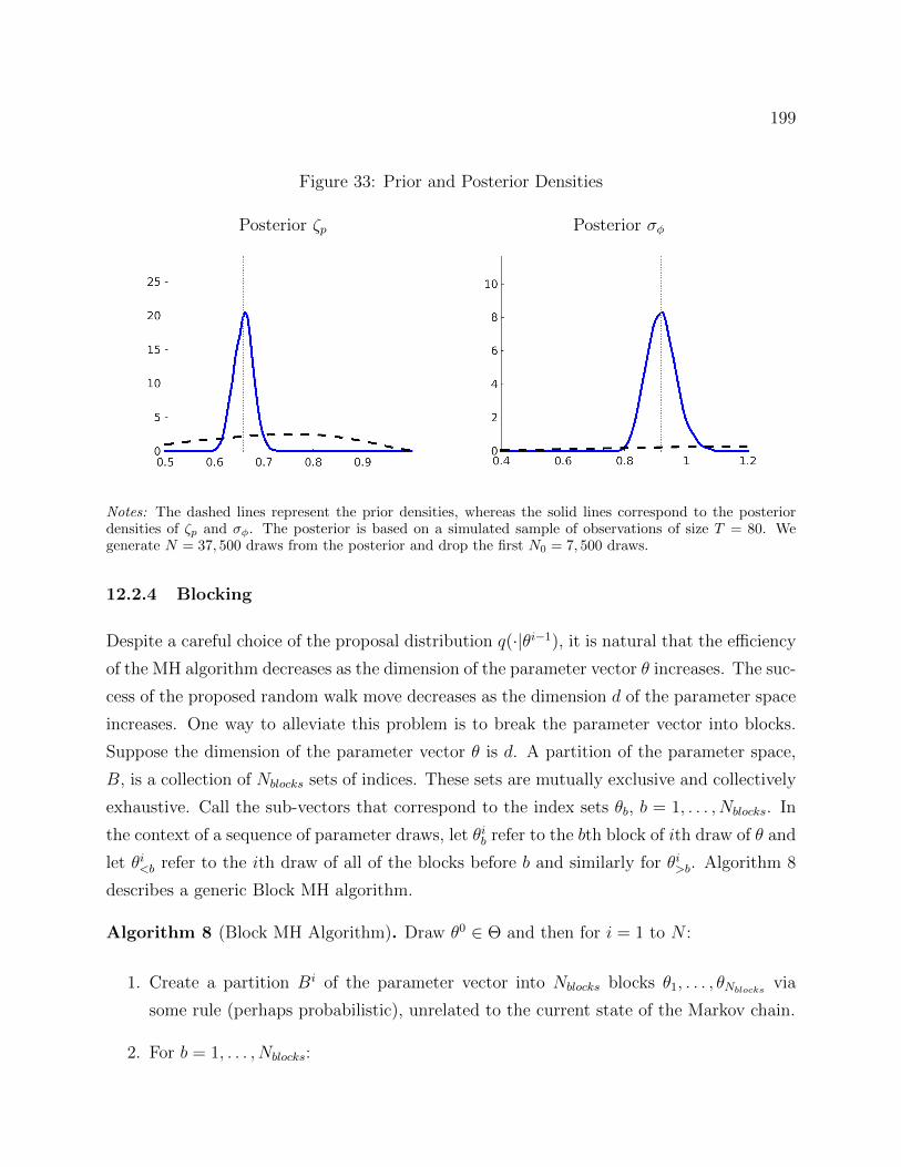
199

Figure 33: Prior and Posterior Densities

Posterior ζp Posterior σφ

Notes: The dashed lines represent the prior densities, whereas the solid lines correspond to the posteriordensities of ζp and σφ. The posterior is based on a simulated sample of observations of size T = 80. Wegenerate N = 37, 500 draws from the posterior and drop the first N0 = 7, 500 draws.

12.2.4 Blocking

Despite a careful choice of the proposal distribution q(·|θi−1), it is natural that the efficiency

of the MH algorithm decreases as the dimension of the parameter vector θ increases. The suc-

cess of the proposed random walk move decreases as the dimension d of the parameter space

increases. One way to alleviate this problem is to break the parameter vector into blocks.

Suppose the dimension of the parameter vector θ is d. A partition of the parameter space,

B, is a collection of Nblocks sets of indices. These sets are mutually exclusive and collectively

exhaustive. Call the sub-vectors that correspond to the index sets θb, b = 1, . . . , Nblocks. In

the context of a sequence of parameter draws, let θib refer to the bth block of ith draw of θ and

let θi<b refer to the ith draw of all of the blocks before b and similarly for θi>b. Algorithm 8

describes a generic Block MH algorithm.

Algorithm 8 (Block MH Algorithm). Draw θ0 ∈ Θ and then for i = 1 to N :

1. Create a partition Bi of the parameter vector into Nblocks blocks θ1, . . . , θNblocks via

some rule (perhaps probabilistic), unrelated to the current state of the Markov chain.

2. For b = 1, . . . , Nblocks:

200

(a) Draw ϑb ∼ q(·|[θi<b, θ

i−1b , θi−1

≥b]).

(b) With probability,

α = max

p([θi<b, ϑb, θ

i−1>b

]|Y )q(θi−1

b , |θi<b, ϑb, θi−1>b )

p(θi<b, θi−1b , θi−1

>b |Y )q(ϑb|θi<b, θi−1b , θi−1

>b ), 1

,

set θib = ϑb, otherwise set θib = θi−1b .

In order to make the Block MH algorithm operational, the researcher has to decide how

to allocate parameters to blocks in each iteration and how to choose the proposal distribution

q(·|[θi<b, θ

i−1b , θi−1

>b

]) for parameters of block b.

A good rule of thumb, however, is that we want the parameters within a block, say, θb, to

be as correlated as possible, while we want the parameters between blocks, say, θb and θ−b,

to be as independent as possible, according to Robert and Casella (2004). Unfortunately,

picking the “optimal” blocks to minimize dependence across blocks requires a priori knowl-

edge about the posterior and is therefore often infeasible. Chib and Ramamurthy (2010)

propose grouping parameters randomly. Essentially, the user specifies how many blocks to

partition the parameter vector into and every iteration a new set of blocks is constructed.

Key to the algorithm is that the block configuration be independent of the Markov chain.

This is crucial for ensuring the convergence of the chain.

In order to tailor the block-specific proposal distributions, Chib and Ramamurthy (2010)

advocate using an optimization routine – specifically, simulated annealing – to find the mode

of the conditional posterior distribution. As in the RWMH-V algorithm, the variance of the

proposal distribution is based on the inverse Hessian of the conditional log posterior density

evaluated at the mode. Unfortunately, the tailoring requires many likelihood evaluations

that slow down the algorithm and a simpler procedure, such as using marginal or conditional

covariance matrices from an initial approximation of the joint posterior covariance matrix,

might be computationally more efficient.

12.2.5 Marginal Likelihood Approximations

The computations thus far do not rely on the marginal likelihood p(Y ), which appears in

the denominator of Bayes Theorem. Marginal likelihoods play an important role in assessing

201

the relative fit of models because they are used to turn prior model probabilities into pos-

terior probabilities. The most widely used marginal likelihood approximation in the DSGE

model literature is the modified harmonic mean estimator proposed by Geweke (1999). This

estimator is based on the identity∫f(θ)

p(Y )dθ =

∫f(θ)

p(Y |θ)p(θ)p(θ|Y )dθ, (12.7)

where f(θ) has the property that∫f(θ)dθ = 1. The identity is obtained by rewriting Bayes

Theorem, multiplying both sides with f(θ) and integrating over θ. Realizing that the left-

hand side simplifies to 1/p(Y ) and that the right-hand side can be approximated by a Monte

Carlo average we obtain

pHM(Y ) =

[1

N

N∑i=1

f(θi)

p(Y |θi)p(θi)

]−1

, (12.8)

where the θi’s are drawn from the posterior p(θ|Y ). The function f(θ) should be chosen to

keep the variance of f(θi)/p(Y |θi)p(θi) small. Geweke (1999) recommends using for f(θ) a

truncated normal approximation of the posterior distribution for θ that is computed from the

output of the posterior sampler. Alternative methods to approximate the marginal likelihood

are discussed in Chib and Jeliazkov (2001), Sims, Waggoner, and Zha (2008), and Ardia,

Basturk, Hoogerheide, and van Dijk (2012). An and Schorfheide (2007) and Herbst and

Schorfheide (2015) provide accuracy comparisons of alternative methods.

12.2.6 Extensions

The basic estimation approach for linearized DSGE models has been extended in several

dimensions. Typically, the parameter space is restricted to a subspace in which a linearized

model has a unique non-explosive rational expectations solution (determinacy). Lubik and

Schorfheide (2004) relax this restriction and also consider the region of the parameter space

in which the solution is indeterminate. By computing the posterior probability of parameter

values associated with indeterminacy, they are able to conduct a posterior odds assessment

of determinacy versus indeterminacy. Justiniano and Primiceri (2008) consider a linearized

DSGE model with structural shocks that exhibit stochastic volatility and develop an MCMC

algorithm for posterior inference. A further extension is provided by Curdia, Del Negro, and

Greenwald (2014), who also allow for shocks that, conditional on the volatility process, have

202

a fat-tailed student-t distribution to capture extreme events such as the Great Recession.

Schorfheide (2005a) and Bianchi (2013) consider the estimation of linearized DSGE models

with regime switching in the coefficients of the state-space representation.

Muller (2012) provides an elegant procedure to assess the robustness of posterior inference

to shifts in the mean of the prior distribution. One of the attractive features of his procedure

is that the robustness checks can be carried out without having to reestimate the DSGE

model under alternative prior distributions. Koop, Pesaran, and Smith (2013) propose some

diagnostics that allow users to determine the extent to which the likelihood function is

informative about the DSGE model parameters. In a nutshell, the authors recommend

examining whether the variance of marginal posterior distributions shrinks at the rate T−1

(in a stationary model) if the number of observations is increased in a simulation experiment.

12.2.7 Particle MCMC

We now turn to the estimation of fully non-linear DSGE models. As discussed in Section 10,

for non-linear DSGE models the likelihood function has to be approximated by a non-linear

filter. Embedding a particle filter approximation into an MCMC sampler leads to a so-called

particle MCMC algorithm. We refer to the combination of a particle-filter approximated

likelihood and the MH algorithm as a PFMH algorithm. This idea was first proposed for the

estimation of non-linear DSGE models by Fernandez-Villaverde and Rubio-Ramırez (2007).

The theory underlying the PFMH algorithm is developed in Andrieu, Doucet, and Holen-

stein (2010). Flury and Shephard (2011) discuss non-DSGE applications of particle MCMC

methods in econometrics. The modification of Algorithm 7 is surprisingly simple: one only

has to replace the exact likelihood function p(Y |θ) with the particle filter approximation

p(Y |θ).

Algorithm 9 (PFMH Algorithm). For i = 1 to N :

1. Draw ϑ from a density q(ϑ|θi−1).

2. Set θi = ϑ with probability

α(ϑ|θi−1) = min

1,

p(Y |ϑ)p(ϑ)/q(ϑ|θi−1)

p(Y |θi−1)p(θi−1)/q(θi−1|ϑ)

and θi = θi−1 otherwise. The likelihood approximation p(Y |ϑ) is computed using

Algorithm 6.

203

The surprising implication of the theory developed in Andrieu, Doucet, and Holenstein

(2010) is that the distribution of draws generated by Algorithm 9 from the PFMH algorithm

that replaces p(Y |θ) with p(Y |θ) in fact does converge to the exact posterior. The replace-

ment of the exact likelihood function by the particle-filter approximation generally increases

the persistence of the Markov chain and makes Monte Carlo approximations less accurate;

see Herbst and Schorfheide (2015) for numerical illustrations. Formally, the key requirement

is that the particle-filter approximation provide an unbiased estimate of the likelihood func-

tion. In practice it has to be ensured that the variance of the numerical approximation is

small relative to the expected magnitude of the differential between p(Y |θi−1) and p(Y |ϑ) in

an ideal version of the algorithm in which the likelihood could be evaluated exactly. Thus,

before embedding the particle-filter approximation into a likelihood function, it is important

to assess its accuracy for low- and high-likelihood parameter values.

12.3 SMC Methods

Sequential Monte Carlo (SMC) techniques to generate draws from posterior distributions of

a static parameter θ are emerging as an attractive alternative to MCMC methods. SMC

algorithms can be easily parallelized and, properly tuned, may produce more accurate ap-

proximations of posterior distributions than MCMC algorithms. Chopin (2002) showed how

to adapt the particle filtering techniques discussed in Section 10.3 to conduct posterior infer-

ence for a static parameter vector. Textbook treatments of SMC algorithms can be found,

for instance, in Liu (2001) and Cappe, Moulines, and Ryden (2005).

The first paper that applied SMC techniques to posterior inference in a small-scale DSGE

models was Creal (2007). Herbst and Schorfheide (2014) develop the algorithm further,

provide some convergence results for an adaptive version of the algorithm building on the

theoretical analysis of Chopin (2004), and show that a properly tailored SMC algorithm

delivers more reliable posterior inference for large-scale DSGE models with a multimodal

posterior than the widely used RWMH-V algorithm. Creal (2012) provides a recent survey

of SMC applications in econometrics. Durham and Geweke (2014) show how to parallelize a

flexible and self-tuning SMC algorithm for the estimation of time series models on graphical

processing units (GPU). The remainder of this section draws heavily from the more detailed

exposition in Herbst and Schorfheide (2014, 2015).

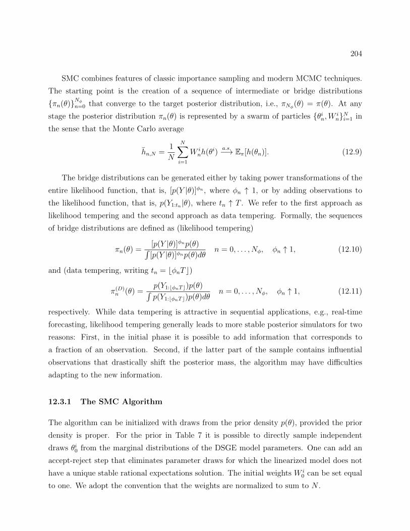
204

SMC combines features of classic importance sampling and modern MCMC techniques.

The starting point is the creation of a sequence of intermediate or bridge distributions

πn(θ)Nφn=0 that converge to the target posterior distribution, i.e., πNφ(θ) = π(θ). At any

stage the posterior distribution πn(θ) is represented by a swarm of particles θin,W inNi=1 in

the sense that the Monte Carlo average

hn,N =1

N

N∑i=1

W inh(θi)

a.s.−→ Eπ[h(θn)]. (12.9)

The bridge distributions can be generated either by taking power transformations of the

entire likelihood function, that is, [p(Y |θ)]φn , where φn ↑ 1, or by adding observations to

the likelihood function, that is, p(Y1:tn|θ), where tn ↑ T . We refer to the first approach as

likelihood tempering and the second approach as data tempering. Formally, the sequences

of bridge distributions are defined as (likelihood tempering)

πn(θ) =[p(Y |θ)]φnp(θ)∫[p(Y |θ)]φnp(θ)dθ n = 0, . . . , Nφ, φn ↑ 1, (12.10)

and (data tempering, writing tn = bφnT c)

π(D)n (θ) =

p(Y1:bφnT c)p(θ)∫p(Y1:bφnT c)p(θ)dθ

n = 0, . . . , Nφ, φn ↑ 1, (12.11)

respectively. While data tempering is attractive in sequential applications, e.g., real-time

forecasting, likelihood tempering generally leads to more stable posterior simulators for two

reasons: First, in the initial phase it is possible to add information that corresponds to

a fraction of an observation. Second, if the latter part of the sample contains influential

observations that drastically shift the posterior mass, the algorithm may have difficulties

adapting to the new information.

12.3.1 The SMC Algorithm

The algorithm can be initialized with draws from the prior density p(θ), provided the prior

density is proper. For the prior in Table 7 it is possible to directly sample independent

draws θi0 from the marginal distributions of the DSGE model parameters. One can add an

accept-reject step that eliminates parameter draws for which the linearized model does not

have a unique stable rational expectations solution. The initial weights W i0 can be set equal

to one. We adopt the convention that the weights are normalized to sum to N .

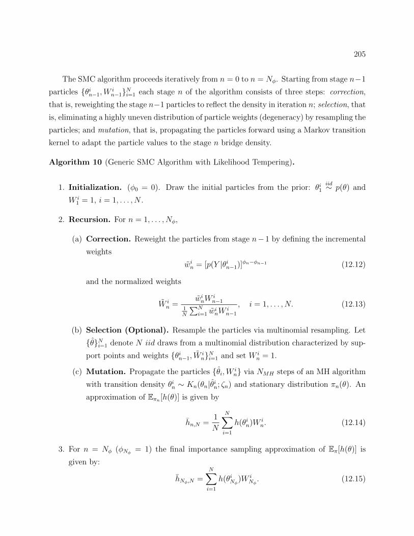
205

The SMC algorithm proceeds iteratively from n = 0 to n = Nφ. Starting from stage n−1

particles θin−1,Win−1Ni=1 each stage n of the algorithm consists of three steps: correction,

that is, reweighting the stage n−1 particles to reflect the density in iteration n; selection, that

is, eliminating a highly uneven distribution of particle weights (degeneracy) by resampling the

particles; and mutation, that is, propagating the particles forward using a Markov transition

kernel to adapt the particle values to the stage n bridge density.

Algorithm 10 (Generic SMC Algorithm with Likelihood Tempering).

1. Initialization. (φ0 = 0). Draw the initial particles from the prior: θi1iid∼ p(θ) and

W i1 = 1, i = 1, . . . , N .

2. Recursion. For n = 1, . . . , Nφ,

(a) Correction. Reweight the particles from stage n− 1 by defining the incremental

weights

win = [p(Y |θin−1)]φn−φn−1 (12.12)

and the normalized weights

W in =

winWin−1

1N

∑Ni=1 w

inW

in−1

, i = 1, . . . , N. (12.13)

(b) Selection (Optional). Resample the particles via multinomial resampling. Let

θNi=1 denote N iid draws from a multinomial distribution characterized by sup-

port points and weights θin−1, WinNi=1 and set W i

n = 1.

(c) Mutation. Propagate the particles θi,W in via NMH steps of an MH algorithm

with transition density θin ∼ Kn(θn|θin; ζn) and stationary distribution πn(θ). An

approximation of Eπn [h(θ)] is given by

hn,N =1

N

N∑i=1

h(θin)W in. (12.14)

3. For n = Nφ (φNφ = 1) the final importance sampling approximation of Eπ[h(θ)] is

given by:

hNφ,N =N∑i=1

h(θiNφ)W iNφ. (12.15)

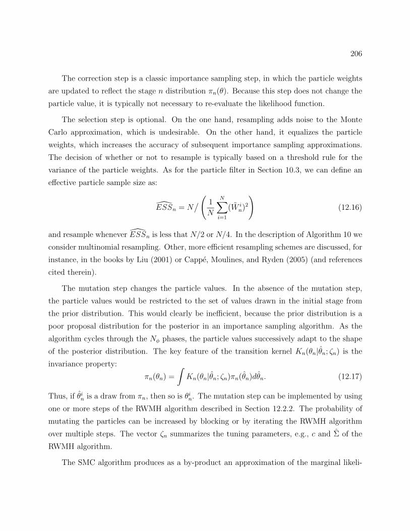
206

The correction step is a classic importance sampling step, in which the particle weights

are updated to reflect the stage n distribution πn(θ). Because this step does not change the

particle value, it is typically not necessary to re-evaluate the likelihood function.

The selection step is optional. On the one hand, resampling adds noise to the Monte

Carlo approximation, which is undesirable. On the other hand, it equalizes the particle

weights, which increases the accuracy of subsequent importance sampling approximations.

The decision of whether or not to resample is typically based on a threshold rule for the

variance of the particle weights. As for the particle filter in Section 10.3, we can define an

effective particle sample size as:

ESSn = N/( 1

N

N∑i=1

(W in)2

)(12.16)

and resample whenever ESSn is less that N/2 or N/4. In the description of Algorithm 10 we

consider multinomial resampling. Other, more efficient resampling schemes are discussed, for

instance, in the books by Liu (2001) or Cappe, Moulines, and Ryden (2005) (and references

cited therein).

The mutation step changes the particle values. In the absence of the mutation step,

the particle values would be restricted to the set of values drawn in the initial stage from

the prior distribution. This would clearly be inefficient, because the prior distribution is a

poor proposal distribution for the posterior in an importance sampling algorithm. As the

algorithm cycles through the Nφ phases, the particle values successively adapt to the shape

of the posterior distribution. The key feature of the transition kernel Kn(θn|θn; ζn) is the

invariance property:

πn(θn) =

∫Kn(θn|θn; ζn)πn(θn)dθn. (12.17)

Thus, if θin is a draw from πn, then so is θin. The mutation step can be implemented by using

one or more steps of the RWMH algorithm described in Section 12.2.2. The probability of

mutating the particles can be increased by blocking or by iterating the RWMH algorithm

over multiple steps. The vector ζn summarizes the tuning parameters, e.g., c and Σ of the

RWMH algorithm.

The SMC algorithm produces as a by-product an approximation of the marginal likeli-

207

hood. It can be shown that

pSMC(Y ) =

Nφ∏n=1

(1

N

N∑i=1

winWin−1

)

converges almost surely to p(Y ) as the number of particles N −→∞.

12.3.2 Tuning the SMC Algorithm

The implementation of the SMC algorithm requires the choice of several tuning constants.

The most important choice is the number of particles N . As shown in Chopin (2004),

Monte Carlo averages computed from the output of the SMC algorithm satisfy a CLT as the

number of particles increases to infinity. This means that the variance of the Monte Carlo

approximation decreases at the rate 1/N . The user has to determine the number of bridge

distributions Nφ and the tempering schedule φn. Based on experiments with a small-scale

DSGE model, Herbst and Schorfheide (2015) recommend a convex tempering schedule of

the form φn = (n/Nφ)λ with λ ≈ 2. Durham and Geweke (2014) recently developed a self-

tuning algorithm that chooses the sequence φn adaptively as the algorithm cycles through

the stages.

The mutation step requires the user to determine the number of MH steps NMH and

the number of parameter blocks. The increased probability of mutation raises the accuracy

but unfortunately, the number of likelihood evaluations increases as well, which slows down

the algorithm. The scaling constant c and the covariance matrix Σ can be easily chosen

adaptively. Based on the MH rejection frequency, c can be adjusted to achieve a target

rejection rate of approximately 25-40%. For Σn one can use an approximation of the posterior

covariance matrix computed at the end of the stage n correction step.

To monitor the accuracy of the SMC approximations Durham and Geweke (2014) suggest

creating H groups of N particles and setting up the algorithm so that there is no commu-

nication across groups. This leads to H Monte Carlo approximations of posterior moments

of interest. The across-group standard deviation of within-group Monte Carlo averages pro-

vides a measure of numerical accuracy. Parallelization of the SMC algorithm is relatively

straightforward because the mutation step and the computation of the incremental weights

in the correction step can be carried out in parallel on multiple processors, each of which is

assigned a group of particles. In principle, the exact likelihood function can be replaced by

208

a particle-filter approximation, which leads to an SMC2 algorithm, developed by Chopin,

Jacob, and Papaspiliopoulos (2012) and discussed in more detail in the context of DSGE

models in Herbst and Schorfheide (2015).

12.3.3 Numerical Illustration

We now illustrate the SMC model in the context of the stylized DSGE models. The set-up is

similar to the one in Section 12.2.3. We generate T = 80 observations using the parameters

listed in Table 5 and use the prior distribution given in Table 7. The algorithm is configured

as follows. We use N = 2, 048 particles and Nφ = 500 tempering stages. We set λ = 3,

meaning that we add very little information in the initial stages to ensure that the prior draws

adapt to the shape of the posterior. We use one step of a single-block RWMH algorithm in

the mutation step and choose c and Σn adaptively as described in Herbst and Schorfheide

(2014). The target acceptance rate for the mutation step is 0.25. Based on the output of the

SMC algorithm, we plot marginal bridge densities πn(·) for the price stickiness parameter ζp

and the shock standard deviation σφ in Figure 34. The initial set of particles is drawn from

the prior distribution. As φn increases to one, the distribution concentrates. The final stage

approximates the posterior distribution.

12.4 Model Diagnostics

DSGE models provide stylized representations of the macroeconomy. To examine whether a

specific model is able to capture salient features of the data Y from an a priori perspective,

prior predictive checks provide an attractive diagnostic. Prior (and posterior) predictive

checks are discussed in general terms in the textbooks by Lancaster (2004) and Geweke

(2005). The first application of a prior predictive check in the context of DSGE models is

Canova (1994).

Let Y ∗1:T be an artificial sample of length T . The predictive distribution for Y ∗1:T based

on the time t information set Ft is

p(Y ∗1:T |Ft) =

∫p(Y ∗1:T |θ)p(θ|Ft)dθ. (12.18)

We used a slightly more general notation (to accommodate posterior predictive checks below)

with the convention that F0 corresponds to prior information. The idea of a predictive

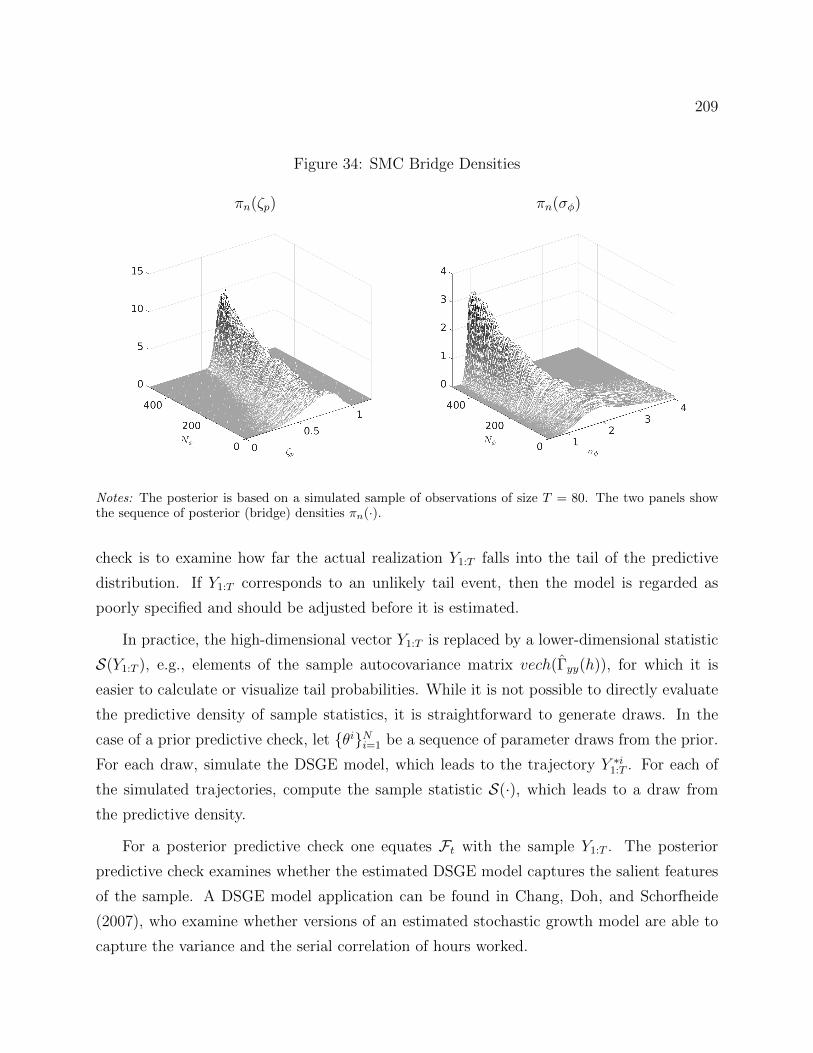
209

Figure 34: SMC Bridge Densities

πn(ζp) πn(σφ)

Notes: The posterior is based on a simulated sample of observations of size T = 80. The two panels showthe sequence of posterior (bridge) densities πn(·).

check is to examine how far the actual realization Y1:T falls into the tail of the predictive

distribution. If Y1:T corresponds to an unlikely tail event, then the model is regarded as

poorly specified and should be adjusted before it is estimated.

In practice, the high-dimensional vector Y1:T is replaced by a lower-dimensional statistic

S(Y1:T ), e.g., elements of the sample autocovariance matrix vech(Γyy(h)), for which it is

easier to calculate or visualize tail probabilities. While it is not possible to directly evaluate

the predictive density of sample statistics, it is straightforward to generate draws. In the

case of a prior predictive check, let θiNi=1 be a sequence of parameter draws from the prior.

For each draw, simulate the DSGE model, which leads to the trajectory Y ∗i1:T . For each of

the simulated trajectories, compute the sample statistic S(·), which leads to a draw from

the predictive density.

For a posterior predictive check one equates Ft with the sample Y1:T . The posterior

predictive check examines whether the estimated DSGE model captures the salient features

of the sample. A DSGE model application can be found in Chang, Doh, and Schorfheide

(2007), who examine whether versions of an estimated stochastic growth model are able to

capture the variance and the serial correlation of hours worked.

210

12.5 Limited Information Bayesian Inference

Bayesian inference requires a likelihood function p(Y |θ). However, as discussed in Section 11,

many of the classical approaches to DSGE model estimation, e.g., (generalized) methods of

moments and impulse response function matching, do not utilize the likelihood function

of the DSGE model, in part because there is some concern about misspecification. These

methods are referred to as limited-information (instead of full-information) techniques. This

subsection provides a brief survey of Bayesian approaches to limited-information inference.

12.5.1 Single-Equation Estimation

Lubik and Schorfheide (2005) estimate monetary policy rules for small open economy models

by augmenting the policy rule equation with a vector-autoregressive law of motion for the

endogenous regressors, e.g., the output gap and inflation in the case of our stylized model.

This leads to a VAR for output, inflation, and interest rates, with cross-coefficient restrictions

that are functions of the monetary policy rule parameters. The restricted VAR can be

estimated with standard MCMC techniques. Compared to the estimation of a fully specified

DSGE model, the limited-information approach robustifies the estimation of the policy rule

equation against misspecification of the private sector’s behavior. Kleibergen and Mavroeidis

(2014) apply a similar technique to the estimation of a New Keynesian Phillips curve. Their

work focuses on the specification of prior distributions that regularize the likelihood function

in settings in which the sample only weakly identifies the parameters of interest, e.g., the

slope of the New Keynesian Phillips curve.

12.5.2 Inverting a Sampling Distribution

Suppose one knows the sampling distribution p(θ|θ) of an estimator θ. Then, instead of

updating beliefs conditional on the observed sample Y , one could update the beliefs about

θ based on the realization of θ:

p(θ|θ) =p(θ|θ)p(θ)∫p(θ|θ)p(θ)

. (12.19)

This idea dates back at least to Pratt, Raiffa, and Schlaifer (1965) and is useful in situations

in which a variety of different distributions for the sample Y lead to the same distribution

211

of the estimator θ. The drawback of this approach is that a closed-form representation of

the density p(θ|θ) is typically not available.

In practice one could use a simulation-based approximation of p(θ|θ), which is an idea

set forth by Boos and Monahan (1986). Alternatively, one could replace the finite-sample

distribution with a limit distribution, e.g.,

√T (θT − θT )|θT =⇒ N

(0, V (θ)

), (12.20)

where the sequence of “true” parameters θT converges to θ. This approach is considered

by Kwan (1999). In principle θT could be any of the frequentist estimators studied in

Section 11 for which we derived an asymptotic distribution, including the MD estimator,

the IRF matching estimator, or the GMM estimator. However, in order for the resulting

limited-information posterior to be meaningful, it is important that the convergence to the

asymptotic distribution be uniform in θ, which requires (12.20) to hold for each sequence

θT −→ θ. A uniform convergence to a normal distribution is typically not attainable as θT

approaches the boundary of the region of the parameter space in which the time series Y1:T

is stationary.

Rather than making statements about the approximation of the limited-information

posterior distribution p(θ|θ), Muller (2013) adopts a decision-theoretic framework and shows

that decisions based on the quasi-posterior that is obtained by inverting the limit distribution

of θT |θ are asymptotically optimal (in the sense that they minimize expected loss) under fairly

general conditions. Suppose that the likelihood function of a DSGE model is misspecified.

In this case the textbook analysis of the ML estimator in Section 11.1 has to be adjusted as

follows. The information matrix equality that ensures that ‖−∇2θ`T (θ|Y )−I(θ0)‖ converges

to zero is no longer satisfied. If we let D = plimT−→∞−∇2θ`T (θ|Y ), then the asymptotic vari-

ance of the ML estimator takes the sandwich form DI(θ0)D′. Under the limited-information

approach coverage sets for individual DSGE model parameters would be computed based

on the diagonal elements of DI(θ0)D′, whereas under a full-information Bayesian approach

with misspecified likelihood function, the coverage sets would (asymptotically) be based on

I−1(θ0). Thus, the limited-information approach robustifies the coverage sets against model

misspecification.

Instead of inverting a sampling distribution of an estimator, one could also invert the

sampling distribution of some auxiliary sample statistic ϕ(Y ). Not surprisingly, the main

212

obstacle is the characterization of the distribution ϕ|θ. A collection of methods referred to

as approximate Bayesian computations (ABC) use a simulation approximation of p(ϕ|θ) and

they could be viewed as a Bayesian version of indirect inference. These algorithms target

pδABC(θ, ϕ∗|ϕ) ∝ p(ϕ∗|θ)p(θ)I‖ϕ∗ − ϕ‖ ≤ δ, (12.21)

where ϕ refers to the auxiliary statistic computed from the observed data, ϕ∗ is the auxiliary

statistic computed from data simulated from the model conditional on a parameter θ, and δ

is the level of tolerance for discrepancies between model-simulated and observed statistics.

To date, there are few applications of ABC in econometrics. Forneron and Ng (2015) discuss

the relationship between ABC and the simulated MD estimators introduced in Section 11.2

and Scalone (2015) explores a DSGE model application.

12.5.3 Limited-Information Likelihood Functions

Kim (2002) constructs a limited-information likelihood function from the objective function

of an extremum estimator. For illustrative purposes we consider the GMM estimator dis-

cussed in Section 11.4, but the same idea can also be applied to the MD estimator and the

IRF matching estimator. Suppose the data are generated under the probability measure

P and at θ = θ0 the following GMM moment condition is satisfied: EP[g(yt−p:t|θ0)] = 0.

The sample objective function QT (θ|Y ) for the resulting GMM estimator based on a weight

matrix W was given in (11.40). Assuming uniform integrability of the sample objective

function

limT−→∞

EP[QT (θ0|Y )] = r (12.22)

where r is the number of overidentifying moment conditions (meaning the difference be-

tween the number of moments stacked in the vector g(·) and the number of elements of the

parameter vector θ).

Let P(θ) denote the collection of probability distributions that satisfy the moment con-

ditions in the following sense:

P(θ) =P | lim

T−→∞EP [TQT (θ|Y )] = k

. (12.23)

P(θ) cannot be used directly for likelihood-based inference because it comprises a collection of

probability distributions indexed by θ. To obtain a unique distribution for each θ, Kim (2002)

213

projects the “true” distribution P onto the set P(θ) using the Kullback-Leibler discrepancy

as the metric:

P ∗(Y |θ) = argminP∈P(θ)

∫log(dP/dP)dP, (12.24)

The solution takes the convenient form

p∗(Y |θ) ∝ exp

−1

2QT (θ|Y )

, (12.25)

where p∗(Y |θ) = dP/dP is the Radon-Nikodym derivative of P with respect to P.

Kim’s (2002) results suggest that the frequentist objective functions of Sections 11.2

to 11.4 can be combined with a prior density and used for (limited-information) Bayesian

inference. The posterior mean

θ =

∫θ exp

−1

2QT (θ|Y )

p(θ)dθ∫

exp−1

2QT (θ|Y )

p(θ)dθ

(12.26)

resembles the LT estimator discussed in Section 11.2. The main difference is that the LT

estimator was interpreted from a frequentist perspective, whereas the quasi-posterior based

on p∗(Y |θ) and statistics such as the posterior mean are meant to be interpreted from a

Bayesian perspective. This idea has been recently exploited by Christiano, Trabandt, and

Walentin (2010) to propose a Bayesian IRF matching estimator. An application to an asset

pricing model is presented in Gallant (2015) and an extension to models with latent variables

is provided in Gallant, Giacomini, and Ragusa (2013). Inoue and Shintani (2014) show that

the limited information marginal likelihood

p∗(Y |M) =

∫p∗(Y |θ,M)p(θ)dθ

can be used as a model selection criterion that asymptotically is able to select a correct

model specification.

12.5.4 Non-parametric Likelihood Functions

There is also a literature on non-parametric likelihood functions that are restricted to satisfy

model-implied moment conditions. Lazar (2003) and Schennach (2005) use empirical likeli-

hood functions, which, roughly speaking assign probability pt to observation yt such that the

likelihood function is written as∏T

t=1 pt, at least if the data are iid. One then imposes the

side constraint∑T

t=1 ptg(yt−p:t|θ) = 0 and concentrates out pt probabilities to obtain a profile

214

objective function that only depends on θ. This method is designed for iid data and possible

models in which g(yt−p:t|θ) is a martingale difference sequence. Kitamura and Otsu (2011)

propose to using a Dirichlet process to generate a prior for the distribution of Y1:T and then

project this distribution on the set of distributions that satisfies the moment restrictions.

Shin (2014) uses a Dirichlet process mixture and provides a time series extension.

13 Conclusion

Over the past two decades the development and application of solution and estimation meth-

ods for DSGE models have experienced tremendous growth. Part of this growth has been

spurred by central banks, which have included DSGE models in their suites of models used for

forecasting and policy analysis. The rapid rise of computing power has enabled researchers

to study more and more elaborate model specifications. As we have been writing this chap-

ter, new methods have been developed and novel applications have been explored. While it

is impossible to provide an exhaustive treatment of such a dynamic field, we hope that this

chapter provides a thorough training for those who are interested in working in this area

and a good overview of the state of the art as of 2015, and inspires innovative research that

expands the frontier of knowledge.

215

References

Aldrich, E. M. (2014): “GPU Computing in Economics,” in Handbook of Computational

Economics, ed. by K. Schmedders, and K. L. Judd, vol. 3, pp. 557–598. Elsevier.

Aldrich, E. M., J. Fernandez-Villaverde, A. R. Gallant, and J. F. Rubio-

Ramırez (2011): “Tapping the Supercomputer Under Your Desk: Solving Dynamic Equi-

librium Models with Graphics Processors,” Journal of Economic Dynamics and Control,

35, 386–393.

Aldrich, E. M., and H. Kung (2011): “Computational Methods for Production-Based

Asset Pricing Models with Recursive Utility,” Economic Research Initiatives at Duke

(ERID) Working Paper, 87.

Algan, Y., O. Allais, W. J. Den Haan, and P. Rendahl (2014): “Solving and

Simulating Models with Heterogeneous Agents and Aggregate Uncertainty,” in Handbook

of Computational Economics, ed. by K. Schmedders, and K. L. Judd, vol. 3, pp. 277–324.

Elsevier.

Altig, D., L. Christiano, M. Eichenbaum, and J. Linde (2011): “Firm-Specific

Capital, Nominal Rigidities and the Business Cycle,” Review of Economic Dynamics,

14(2), 225–247.

Altug, S. (1989): “Time-to-Build and Aggregate Fluctuations: Some New Evidence,”

International Economic Review, 30(4), 889–920.

Alvarez, F., and U. J. Jermann (2004): “Using Asset Prices to Measure the Cost of

Business Cycles,” Journal of Political Economy, 112, 1223–1256.

An, S., and F. Schorfheide (2007): “Bayesian Analysis of DSGE Models,” Econometric

Reviews, 26(2-4), 113–172.

Anderson, E. W., L. P. Hansen, E. R. McGrattan, and T. J. Sargent (1996):

“On the Mechanics of Forming and Estimating Dynamic Linear Economies,” in Handbook

of Computational Economics, ed. by H. M. Amman, D. A. Kendrick, and J. Rust, vol. 1,

pp. 171–252. Elsevier.

216

Andreasen, M. M. (2013): “Non-Linear DSGE Models and the Central Difference Kalman

Filter,” Journal of Applied Econometrics, 28(6), 929–955.

Andreasen, M. M., J. Fernandez-Villaverde, and J. F. Rubio-Ramırez (2013):

“The Pruned State-Space System for Nonlinear DSGE Models: Theory and Empircal

Applications,” NBER Working, 18983.

Andrews, I., and A. Mikusheva (2015): “Maximum Likelihood Inference in Weakly

Identified DSGE Models,” Quantitative Economics, forthcoming.

Andrieu, C., A. Doucet, and R. Holenstein (2010): “Particle Markov Chain Monte

Carlo Methods,” Journal of the Royal Statistical Society Series B, 72(3), 269–342.

Ardia, D., N. Basturk, L. Hoogerheide, and H. K. van Dijk (2012): “A Com-

parative Study of Monte Carlo Methods for Efficient Evaluation of Marginal Likelihood,”

Computational Statistics and Data Analysis, 56(11), 3398–3414.

Arulampalam, S., S. Maskell, N. Gordon, and T. Clapp (2002): “A Tutorial on

Particle Filters for Online Nonlinear/Non-Gaussian Bayesian Tracking,” IEEE Transac-

tions on Signal Processing, 50(2), 174–188.

Aruoba, S. B., J. Fernandez-Villaverde, and J. F. Rubio-Ramırez (2006): “Com-

paring Solution Methods for Dynamic Equilibrium Economies,” Journal of Economic Dy-

namics and Control, 30(12), 2477–2508.

Aruoba, S. B., and F. Schorfheide (2015): “Inflation During and After the Zero Lower

Bound,” Manuscript, University of Maryland.

Barthelmann, V., E. Novak, and K. Ritter (2000): “High Dimensional Polynomial

Interpolation on Sparse Grids,” Advances in Computational Mathematics, 12, 273–288.

Bastani, H., and L. Guerrieri (2008): “On the Application of Automatic Differentiation

to the Likelihood Function for Dynamic General Equilibrium Models,” in Advances in

Automatic Differentiation: Lecture Notes in Computational Science and Engineering, ed.

by C. H. Bischof, H. M. Bucker, P. Hovland, U. Naumann, and J. Utke, vol. 64, pp.

303–313. Springer.

217

Bender, C. M., and S. A. Orszag (1999): Advanced Mathematical Methods for Scientists

and Engineers: Asymptotic Methods and Perturbation Theory. Springer.

Benigno, P., and M. Woodford (2004): “Optimal Monetary and Fiscal Policy: A

Linear-Quadratic Approach,” NBER Macroeconomics Annual, 18.

Bernanke, B. S., and M. Gertler (1989): “Agency Costs, Net Worth, and Business

Fluctuations,” American Economic Review, 79(1), 14–31.

Bernanke, B. S., M. Gertler, and S. Gilchrist (1999): “The Financial Accelerator

in a Quantitative Business Cycle Framework,” in Handbook of Macroeconomics, ed. by

J. B. Taylor, and M. Woodford, vol. 1, pp. 1341–1393. Elsevier.

Bianchi, F. (2013): “Regime Switches, Agents’ Beliefs, and Post-World War II U.S.

Macroeconomic Dynamics,” Review of Economic Studies, 80(2), 463–490.

Blanchard, O. J., and C. M. Kahn (1980): “The Solution of Linear Difference Models

under Rational Expectations,” Econometrica, 48(5), 1305–1312.

Bloom, N. (2009): “The Impact of Uncertainty Shocks,” Econometrica, 77, 623–685.

Bocola, L. (2015): “The Pass-Through of Sovereign Risk,” Manuscript, Northwestern

University.

Boos, D. D., and J. F. Monahan (1986): “Bootstrap Methods Using Prior Information,”

Biometrika, 73(1), 77–83.

Boyd, J. P. (2000): Chebyshev and Fourier Spectral Methods. Dover.

Boyd, J. P., and R. G. Petschek (2014): “The Relationships Between Chebyshev,

Legendre and Jacobi Polynomials: The Generic Superiority of Chebyshev Polynomials

and Three Important Exceptions,” Journal of Scientific Computing, 59, 1–27.

Brenner, S., and R. Scott (2008): The Mathematical Theory of Finite Element Methods.

Springer Verlag.

Brown, D. B., J. E. Smith, and S. Peng (2010): “Information Relaxations and Duality

in Stochastic Dynamic Programs,” Operations Research, 4.

218

Brumm, J., and S. Scheidegger (2015): “Using Adaptive Sparse Grids to Solve High-

Dimensional Dynamic Models,” Manuscript, University of Zurich.

Bungartz, H.-J., and M. Griebel (2004): “Sparse Grids,” Acta Numerica, 13, 147–269.

Burnside, C., M. Eichenbaum, and S. Rebelo (1993): “Labor Hoarding and the

Business Cycle,” Journal of Political Economy, 101(2), 245–73.

Cai, Y., and K. L. Judd (2014): “Advances in Numerical Dynamic Programming and

New Applications,” in Handbook of Computational Economics, ed. by K. Schmedders, and

K. L. Judd, vol. 3, pp. 479–516. Elsevier.

Caldara, D., J. Fernandez-Villaverde, J. F. Rubio-Ramırez, and W. Yao (2012):

“Computing DSGE Models with Recursive Preferences and Stochastic Volatility,” Review

of Economic Dynamics, 15, 188–206.

Canova, F. (1994): “Statistical Inference in Calibrated Models,” Journal of Applied Econo-

metrics, 9, S123–144.

(2007): Methods for Applied Macroeconomic Research. Princeton University Press.

(2014): “Bridging Cyclical DSGE Models and the Raw Data,” Journal of Monetary

Economics, 67, 1–15.

Canova, F., and G. De Nicolo (2002): “Monetary Disturbances Matter for Business

Fluctuations in the G-7,” Journal of Monetary Economics, 49(4), 1131–1159.

Canova, F., F. Ferroni, and C. Matthes (2014): “Choosing the Variables to Estimate

Singular DSGE Models,” Journal of Applied Econometrics, 29(7), 1099–1117.

Cappe, O., S. J. Godsill, and E. Moulines (2007): “An Overview of Existing Methods

and Recent Advances in Sequential Monte Carlo,” Proceedings of the IEEE, 95(5), 899–

924.

Cappe, O., E. Moulines, and T. Ryden (2005): Inference in Hidden Markov Models.

Springer Verlag.

Carlstrom, C., and T. S. Fuerst (1997): “Agency Costs, Net Worth, and Business

Fluctuations: A Computable General Equilibrium Analysis,” American Economic Review,

87, 893–910.

219

Chang, Y., T. Doh, and F. Schorfheide (2007): “Non-stationary Hours in a DSGE

Model,” Journal of Money, Credit, and Banking, 39(6), 1357–1373.

Chari, V. V., P. J. Kehoe, and E. R. McGrattan (2008): “Are Structural VARs

with Long-Run Restrictions Useful in Developing Business Cycle Theory?,” Journal of

Monetary Economics, 55(8), 1337–1352.

Chen, X. (2007): “Large Sample Sieve Estimation of Semi-Nonparametric Models,” in

Handbook of Econometrics, ed. by J. J. Heckman, and E. E. Leamer, vol. 6, pp. 5549–

5632. Elsevier.

Chernozhukov, V., and H. Hong (2003): “An MCMC Approach to Classical Estima-

tion,” Journal of Econometrics, 115, 293–346.

Chib, S., and E. Greenberg (1995): “Understanding the Metropolis-Hastings Algo-

rithm,” The American Statistician, 49, 327–335.

Chib, S., and I. Jeliazkov (2001): “Marginal Likelihoods from the Metropolis Hastings

Output,” Journal of the American Statistical Association, 96(453), 270–281.

Chib, S., and S. Ramamurthy (2010): “Tailored Randomized Block MCMC Methods

with Application to DSGE Models,” Journal of Econometrics, 155(1), 19–38.

Cho, J.-O., T. F. Cooley, and H. S. E. Kim (2015): “Business Cycle Uncertainty and

Economic Welfare,” Review of Economic Dynamics, 18, 185–200.

Chopin, N. (2002): “A Sequential Particle Filter for Static Models,” Biometrika, 89(3),

539–551.

(2004): “Central Limit Theorem for Sequential Monte Carlo Methods and its

Application to Bayesian Inference,” Annals of Statistics, 32(6), 2385–2411.

Chopin, N., P. E. Jacob, and O. Papaspiliopoulos (2012): “SMC2: An Efficient

Algorithm for Sequential Analysis of State-Space Models,” arXiv:1101.1528.

Christiano, L. J. (1990): “Linear-Quadratic Approximation and Value-Function Iteration:

A Comparison,” Jornal of Business and Economic Statistics, 8, 99–113.

220

Christiano, L. J., and M. Eichenbaum (1992): “Current Real-Business-Cycle Theories

and Aggregate Labor-Market Fluctuations,” American Economic Review, 82(3), 430–50.

Christiano, L. J., M. Eichenbaum, and C. L. Evans (1999): “Monetary Policy Shocks:

What Have We Learned and to What End,” in Handbook of Macroeconomics, ed. by J. B.

Taylor, and M. Woodford, vol. 1a, chap. 2, pp. 65–148. North Holland, Amsterdam.

(2005): “Nominal Rigidities and the Dynamic Effects of a Shock to Monetary

Policy,” Journal of Political Economy, 113(1), 1–45.

Christiano, L. J., M. Eichenbaum, and S. T. Rebelo (2011): “When Is the Govern-

ment Spending Multiplier Large?,” Jornal of Political Economy, 119.

Christiano, L. J., M. Eichenbaum, and R. Vigfusson (2007): “Assessing Structural

VARs,” in NBER Macroeconomics Annual 2006, ed. by D. Acemoglu, K. Rogoff, and

M. Woodford, vol. 21, pp. 1–72. MIT Press, Cambridge.

Christiano, L. J., and J. D. M. Fisher (2000): “Algorithms for Solving Dynamic Models

with Occasionally Binding Constraints,” Journal of Economic Dynamics and Control, 24,

1179–1232.

Christiano, L. J., R. Motto, and M. Rostagno (2014): “Risk Shocks,” American

Economic Review, 104, 27–65.

Christiano, L. J., M. Trabandt, and K. Walentin (2010): “DSGE Models for Mon-

etary Policy Analysis,” in Handbook of Monetary Economics, ed. by B. M. Friedman, and

M. Woodford, vol. 3 of Handbook of Monetary Economics, chap. 7, pp. 285–367. Elsevier.

Christiano, L. J., and R. J. Vigfusson (2003): “Maximum Likelihood in the Frequency

Domain: The Importance of Time-to-plan,” Journal of Monetary Economics, 50(4), 789–

815.

Clough, R. W. (1960): “The Finite Element Method in Plane Stress Analysis,” Proceedings

of the 2nd ASCE Conference on Electronic Computation.

Clough, R. W., and E. L. Wilson (1999): “Early Finite Element Research at Berkeley,”

Manuscript, University of California, Berkeley.

221

Cochrane, J. H. (1994): “Shocks,” Carnegie Rochester Conference Series on Public Policy,

41(4), 295–364.

(2011): “Determinacy and Identification with Taylor Rules,” Journal of Political

Economy, 119(3), 565 – 615.

Creal, D. (2007): “Sequential Monte Carlo Samplers for Bayesian DSGE Models,”

Manuscript, Chicago Booth.

(2012): “A Survey of Sequential Monte Carlo Methods for Economics and Finance,”

Econometric Reviews, 31(3), 245–296.

Crisan, D., and B. Rozovsky (eds.) (2011): The Oxford Handbook of Nonlinear Filtering.

Oxford University Press.

Curdia, V., M. Del Negro, and D. L. Greenwald (2014): “Rare Shocks, Great

Recessions,” Journal of Applied Econometrics, 29(7), 1031–1052.

DeJong, D. N., and C. Dave (2007): Structural Macroeconometrics. Princeton University

Press.

DeJong, D. N., B. F. Ingram, and C. H. Whiteman (2000): “A Bayesian Approach

to Dynamic Macroeconomics,” Journal of Econometrics, 98(2), 203 – 223.

Del Moral, P. (2004): Feynman-Kac Formulae. Springer Verlag.

(2013): Mean Field Simulation for Monte Carlo Integration. Chapman & Hall/CRC.

Del Negro, M., R. Hasegawa, and F. Schorfheide (2014): “Dynamic Prediction

Pools: An Investigation of Financial Frictions and Forecasting Performance,” NBER

Working Paper, 20575.

Del Negro, M., and F. Schorfheide (2004): “Priors from General Equilibrium Models

for VARs,” International Economic Review, 45(2), 643 – 673.

(2008): “Forming Priors for DSGE Models (and How it Affects the Assessment of

Nominal Rigidities),” Journal of Monetary Economics, 55(7), 1191–1208.

(2009): “Monetary Policy with Potentially Misspecified Models,” American Eco-

nomic Review, 99(4), 1415–1450.

222

(2011): “Bayesian Macroeconometrics,” in Handbook of Bayesian Econometrics,

ed. by H. van Dijk, G. Koop, and J. Geweke, pp. 293–389. Oxford University Press.

(2013): “DSGE Model-Based Forecasting,” in Handbook of Economic Forecasting,

ed. by G. Elliott, and A. Timmermann, vol. 2, pp. 57–140. North Holland, Amsterdam.

Del Negro, M., F. Schorfheide, F. Smets, and R. Wouters (2007): “On the Fit

of New Keynesian Models,” Journal of Business and Economic Statistics, 25(2), 123–162.

Delvos, F.-J. (1982): “d-Variate Boolean Interpolation,” Journal of Approximation The-

ory, 34, 99–114.

Demkowicz, L. (2007): Computing with hp-Adaptive Finite Elements, Volume 1. Chapman

& Hall / CRC.

Den Haan, W. J., and J. De Wind (2012): “Nonlinear and Stable Perturbation-Based

Approximations,” Journal of Economic Dynamics and Control, 36, 1477–1497.

Den Haan, W. J., and A. Marcet (1990): “Solving the Stochastic Growth Model by

Parameterizing Expectations,” Journal of Business and Economic Statistics, 8.

(1994): “Accuracy in Simulations,” Review of Economic Studies, 61, 3–17.

Dıaz-Gimenez, J. (1999): “Linear-Quadratic Approximations: An Introduction,” in Com-

putational Methods for the Study of Dynamic Economies, ed. by R. Marimon, and A. Scott.

Oxford University Press.

Doucet, A., N. de Freitas, and N. Gordon (eds.) (2001): Sequential Monte Carlo

Methods in Practice. Springer Verlag.

Doucet, A., and A. M. Johansen (2011): “A Tutorial on Particle Filtering and Smooth-

ing: Fifteen Years Later,” in Handook of Nonlinear Filtering, ed. by D. Crisan, and B. Ro-

zovsky. Oxford University Press.

Dridi, R., A. Guay, and E. Renault (2007): “Indirect Inference and Calibration of

Dynamic Stochastic General Equilibrium Models,” Journal of Econometrics, 136(2), 397–

430.

223

Dufour, J.-M., L. Khalaf, and M. Kichian (2013): “Identification-Robust Analysis

of DSGE and Structural Macroeconomic Models,” Journal of Monetary Economics, 60,

340–350.

Durbin, J., and S. J. Koopman (2001): Time Series Analysis by State Space Methods.

Oxford University Press.

Durham, G., and J. Geweke (2014): “Adaptive Sequential Posterior Simulators for

Massively Parallel Computing Environments,” Advances in Econometrics, 34, 1–44.

Eggertsson, G. B., and M. Woodford (2003): “The Zero Bound on Interest Rates

and Optimal Monetary Policy,” Brookings Papers on Economic Activity, 34, 139–235.

Epstein, L. G., and S. E. Zin (1989): “Substitution, Risk Aversion, and the Temporal

Behavior of Consumption and Asset Returns: A Theoretical Framework,” Econometrica,

57, 937–969.

Erdos, P., and P. Turan (1937): “On Interpolation I. Quadrature and Mean Convergence

in the Lagrange Interpolation,” Annals of Mathematics, 38, 142–155.

Fair, R. C., and J. B. Taylor (1983): “Solution and Maximum Likelihood Estimation

of Dynamic Nonlinear Rational Expectations Models,” Econometrica, 51, 1169–1185.

Faust, J. (1998): “The Robustness of Identified VAR Conclusions about Money,” Carnegie

Rochester Conference Series on Public Policy, 49(4), 207–244.

Fernandez-Villaverde, J. (2010): “Fiscal Policy in a Model with Financial Frictions,”

American Economic Review Papers and Proceedings, 100.

Fernandez-Villaverde, J., G. Gordon, P. A. Guerron-Quintana, and J. F.

Rubio-Ramırez (2015): “Nonlinear Adventures at the Zero Lower Bound,” Journal of

Economic Dynamics and Control, 57, 182–204.

Fernandez-Villaverde, J., P. A. Guerron-Quintana, and J. F. Rubio-Ramırez

(2014): “Supply-Side Policies and the Zero Lower Bound,” IMF Economic Review, 62(248-

260).

(2015): “Estimating Dynamic Equilibrium Models with Stochastic Volatility,” Jour-

nal of Econometrics, 185, 216–229.

224

Fernandez-Villaverde, J., P. A. Guerron-Quintana, J. F. Rubio-Ramırez, and

M. Uribe (2011): “Risk Matters: The Real Effects of Volatility Shocks,” American

Economic Review, 101, 2530–2561.

Fernandez-Villaverde, J., and O. Levintal (2016): “Solution Methods for Models

with Rare Disasters,” Manuscript, University of Pennsylvania.

Fernandez-Villaverde, J., and J. F. Rubio-Ramırez (2004): “Comparing Dynamic

Equilibrium Models to Data: a Bayesian Approach,” Journal of Econometrics, 123(1),

153 – 187.

(2006): “Solving DSGE Models with Perturbation Methods and a Change of Vari-

ables,” Journal of Economic Dynamics and Control, 30, 2509–2531.

Fernandez-Villaverde, J., and J. F. Rubio-Ramırez (2007): “Estimating Macroeco-

nomic Models: A Likelihood Approach,” Review of Economic Studies, 74(4), 1059–1087.

(2008): “How Structural are Structural Parameters?,” in NBER Macroeconomics

Annual 2007, ed. by D. Acemoglu, K. Rogoff, and M. Woodford, vol. 22. University of

Chicago Press, Chicago, University of Chicago Press.

Fernandez-Villaverde, J., J. F. Rubio-Ramırez, and M. S. S. Santos (2006):

“Convergence Properties of the Likelihood of Computed Dynamic Models,” Econometrica,

74(1), 93–119, RR ReStud.

Fernandez-Villaverde, J., J. F. Rubio-Ramırez, T. J. Sargent, and M. W.

Watson (2007): “ABCs (and Ds) of Understanding VARs,” American Economic Review,

97(3), 1021–1026.

Flury, T., and N. Shephard (2011): “Bayesian Inference Based Only on Simulated

Likelihood: Particle Filter Analysis of Dynamic Economic Models,” Econometric Theory,

27, 933–956.

Fornberg, B. (1996): A Practical Guide to Pseudospectral Methods. Cambridge University

Press.

Forneron, J.-J., and S. Ng (2015): “The ABC of Simulation Estimation with Auxiliary

Statistics,” Manuscript, Columbia University.

225

Gallant, A. R. (2015): “Reflections on the Probability Space Induced by Moment Con-

ditions with Implications for Bayesian Inference,” Journal of Financial Econometrics,

forthcoming.

Gallant, A. R., R. Giacomini, and G. Ragusa (2013): “Generalized Method of Mo-

ments with Latent Variables,” CEPR Discussion Papers, DP9692.

Galor, O. (2007): Discrete Dynamical Systems. Springer.

Gaspar, J., and K. L. Judd (1997): “Solving Large-Scale Rational-Expectations Models,”

Macroeconomic Dynamics, 1, 45–75.

Geweke, J. (1999): “Using Simulation Methods for Bayesian Econometric Models: Infer-

ence, Development, and Communication,” Econometric Reviews, 18(1), 1–126.

(2005): Contemporary Bayesian Econometrics and Statistics. John Wiley & Sons,

Inc.

(2010): Complete and Incomplete Econometric Models. Princeton University Press,

Princeton, New Jersey.

Geweke, J., and G. Amisano (2011): “Optimal Prediction Pools,” Journal of Economet-

rics, 164, 130–141.

(2012): “Prediction with Misspecified Models,” American Economic Review: Pa-

pers & Proceedings, 103(3), 482–486.

Gordon, G. (2011): “Computing Dynamic Heterogeneous-Agent Economies: Tracking the

Distribution,” PIER Working Paper, University of Pennsylvania, 11-018.

Gorodnichenko, Y., and S. Ng (2010): “Estimation of DSGE Models When the Data

are Persistent,” Journal of Monetary Economics, 57(3), 325–340.

Gourieroux, C., A. Monfort, and E. Renault (1993): “Indirect Inference,” Journal

of Applied Econometrics, 8, S85–S118.

Gourieroux, C., P. C. B. Phillips, and J. Yu (2010): “Indirect Inference for Dynamic

Panel Models,” Journal of Econometrics, 157(1), 68–77.

226

Guerron-Quintana, P. A. (2010): “What You Match Does Matter: The Effects of

Observable Variables on DSGE Estimation,” Journal of Applied Econometrics, 25, 774–

804.

Guerron-Quintana, P. A., A. Inoue, and L. Kilian (2013): “Frequentist Inference

in Weakly Identified Dynamic Stochastic General Equilibrium Models,” Quantitative Eco-

nomics, 4, 197–229.

(2014): “Impulse Response Matching Estimators for DSGE Models,” Manuscript,

Federal Reserve Bank of Philadelphia.

Guo, D., X. Wang, and R. Chen (2005): “New Sequential Monte Carlo Methods for

Nonlinear Dynamic Systems,” Statistics and Computing, 15, 135.147.

Hamilton, J. D. (1994): Time Series Analysis. Princeton University Press.

Hansen, G. D., and E. C. Prescott (1995): “Recursive Methods for Computing Equi-

libria of Business Cycle Models,” in Frontiers of Business Cycle Research, ed. by T. F.

Cooley, pp. 39–64. Princeton University Press.

Hansen, L. P. (1982): “Large Sample Properties of Generalized Method of Moments Es-

timators,” Econometrica, 50(4), 1029–54.

Hansen, L. P., J. C. Heaton, and N. Li (2008): “Consumption Strikes Back? Measuring

Long-run Risk,” Journal of Political Economy, 116(2), 260 – 302.

Hansen, L. P., and T. J. Sargent (2013): Recursive Models of Dynamic Linear

Economies. Princeton Press.

Herbst, E., and F. Schorfheide (2014): “Sequential Monte Carlo Sampling for DSGE

Models,” Journal of Applied Econometrics, 29(7), 1073–1098.

(2015): Bayesian Estimation of DSGE Models. Princeton University Press.

Hnatkosvaka, V., V. Marmer, and Y. Tang (2012): “Comparison of Misspecified

Calibrated Models: The Minimum Distance Approach,” Journal of Econometrics, 169(1),

131–138.

227

Hughes, T. J. R. (2000): The Finite Element Method: Linear Static and Dynamic Finite

Element Analysis. Dover.

Hurwicz, L. (1962): “On the Structural Form of Interdependent Systems,” in Logic,

Methodology and Philosophy of Science, ed. by E. Nagel, and A. Tarski. Stanford Uni-

versity Press.

Ingram, B., and C. Whiteman (1994): “Supplanting the Minnesota Prior- Forecasting

Macroeconomic Time Series Using Real Business Cycle Model Priors,” Journal of Mone-

tary Economics, 49(4), 1131–1159.

Inoue, A., and M. Shintani (2014): “Quasi-Bayesian Model Selection,” Manuscript,

Vanderbilt University.

Iskrev, N. (2010): “Local Identification of DSGE Models,” Journal of Monetary Eco-

nomics, 2, 189–202.

Jin, H.-H., and K. L. Judd (2002): “Perturbation Methods for General Dynamic Stochas-

tic Models,” Manuscript, Hoover Institution.

Judd, K. (1998): Numerical Methods in Economics. MIT Press, Cambridge.

Judd, K. L. (1992): “Projection Methods for Solving Aggregate Growth Models,” Journal

of Economic Theory, 58, 410–452.

(2003): “Perturbation Methods with Nonlinear Changes of Variables,” Manuscript,

Hoover Institution.

Judd, K. L., and S.-M. Guu (1993): “Perturbation Solution Methods for Economic

Growth Models,” in Economic and Financial Modeling with Mathematica, ed. by H. Var-

ian, pp. 80–103. Springer Verlag.

(1997): “Asymptotic Methods for Aggregate Growth Models,” Journal of Economic

Dynamics and Control, 21, 1025–1042.

(2001): “Asymptotic Methods for Asset Market Equilibrium Analysis,” Economic

Theory, 18, 127–157.

228

Judd, K. L., L. Maliar, and S. Maliar (2011a): “How to Solve Dynamic Stochastic

Models Computing Expectations Just Once,” NBER Working Paper, 17418.

(2011b): “Numerically Stable and Accurate Stochastic Simulation Methods for

Solving Dynamic Models,” Quantitative Economics, 2, 173–210.

(2014): “Lower Bounds on Approximation Errors: Testing the Hypothesis That a

Numerical Solution Is Accurate,” Manuscript, Hoover Institution.

Judd, K. L., L. Maliar, S. Maliar, and R. Valero (2014): “Smolyak Method for Solv-

ing Dynamic Economic Models: Lagrange Interpolation, Anisotropic Grid and Adaptive

Domain,” Journal of Economic Dynamics and Control, 44, 92–123.

Justiniano, A., and G. E. Primiceri (2008): “The Time-Varying Volatility of Macroe-

conomic Fluctuations,” American Economic Review, 98(3), 604–641.

Kantas, N., A. Doucet, S. Singh, J. Maciejowski, and N. Chopin (2014): “On

Particle Methods for Parameter Estimation in State-Space Models,” arXiv Working Paper,

1412.8659v1.

Kilian, L. (1998): “Small-sample Confidence Intervals for Impulse Response Functions,”

Review of Economics and Statistics, 80(2), 218–230.

(1999): “Finite-Sample Properties of Percentile and Percentile-t Bootstrap Confi-

dence Intervals for Impulse Responses,” Review of Economics and Statistics, 81(4), 652–

660.

Kim, J., and S. H. Kim (2003): “Spurious Welfare Reversals in International Business

Cycle Models,” Journal of International Economics, 60, 471–500.

Kim, J., S. H. Kim, E. Schaumburg, and C. A. Sims (2008): “Calculating and Using

Second-Order Accurate Solutions of Discrete Time Dynamic Equilibrium Models,” Journal

of Economic Dynamics and Control, 32, 3397–3414.

Kim, J.-Y. (2002): “Limited Information Likelihood and Bayesian Analysis,” Journal of

Econometrics, 107(1-2), 175 – 193.

Kimball, M. S. (1990): “Precautionary Saving in the Small and in the Large,” Economet-

rica, 58, 53–73.

229

King, R. G., C. I. Plosser, and S. Rebelo (1988): “Production, Growth, and Business

Cycles: I The Basic Neoclassical Model,” Journal of Monetary Economics, 21(2-3), 195–

232.

King, R. G., C. I. Plosser, and S. T. Rebelo (2002): “Production, Growth and

Business Cycles: Technical Appendix,” Computational Economics, 20, 87–116.

King, R. G., and M. W. Watson (1998): “The Solution of Singular Linear Difference

Systems Under Rational Expectations,” International Economic Review, 39, 1015–1026.

Kitamura, Y., and T. Otsu (2011): “Bayesian Analysis of Moment Condition Models

Using Nonparametric Priors,” Manuscript, Yale University and LSE.

Kleibergen, F., and S. Mavroeidis (2009): “Weak Instrument Robust Tests in GMM

and the New Keynesian Phillips Curve,” Journal of Business & Economic Statistics, 27(3),

293–311.

(2014): “Identification Issues in Limited-Information Bayesian Analysis of Struc-

tural Macroeconomic Models,” Journal of Applied Econometrics, 29, 1183–1209.

Klein, P. (2000): “Using the Generalized Schur Form to Solve a Multivariate Linear Ratio-

nal Expectations Model,” Journal of Economic Dynamics and Control, 24(10), 1405–1423.

Kociecki, A., and M. Kolasa (2015): “Global Identification of Linearized DSGE Mod-

els,” Manuscript, Bank of Poland.

Kogan, L., and I. Mitra (2014): “Accuracy Verification for Numerical Solutions of Equi-

librium Models,” Manuscript, MIT.

Kollmann, R. (2015): “Tractable Latent State Filtering for Non-Linear DSGE Models

Using a Second-Order Approximation and Pruning,” Computational Economics, 45, 239–

260.

Komunjer, I., and S. Ng (2011): “Dynamic Identification of DSGE Models,” Economet-

rica, 79(6), 1995–2032.

Koop, G., H. M. Pesaran, and S. M. Potter (1996): “Impulse Response Analysis in

Nonlinear Multivariate Models,” Journal of Econometrics, 74, 119–147.

230

Koop, G., H. M. Pesaran, and R. P. Smith (2013): “On Identification of Bayesian

DSGE Models,” Journal of Business & Economic Statistics, 31(3), 300–314.

Kopecky, K. A., and R. M. H. Suen (2010): “Finite State Markov-chain Approximations

to Highly Persistent Processes,” Review of Economic Dynamics, 13, 701–714.

Kormilitsina, A., and D. Nekipelov (2012): “Approximation Properties of Laplace-

Type Estimators,” Advances in Econometrics, 28, 291–318.

Kormilitsina, A., and D. Nekipelov (2016): “Consistent Variance of the Laplace Type

Estimators: Application to DSGE Models,” International Economic Review, forthcoming.

Kruger, D., and F. Kubler (2004): “Computing Equilibrium in OLG Models with

Stochastic Production,” Journal of Economic Dynamics and Control, 28, 1411–1436.

Krusell, P., and A. A. Smith (1998): “Income and Wealth Heterogeneity in the Macroe-

conomy,” Journal of Political Economy, 106, 867–896.

Kwan, Y. K. (1999): “Asymptotic Bayesian Analysis Based on a Limited Information

Estimator,” Journal of Econometrics, 88, 99–121.

Kydland, F. E., and E. C. Prescott (1982): “Time to Build and Aggregate Fluctua-

tions,” Econometrica, 50(6), 1345–70.

Lancaster, T. (2004): An Introduction to Modern Bayesian Econometrics. Blackwell Pub-

lishing.

Lanczos, C. (1938): “Trigonometric Interpolation of Empirical and Analytical Functions,”

Journal of Mathematical Physics, 17, 123–199.

Lazar, N. A. (2003): “Bayesian Empirical Likelihood,” Biometrika, 90(2), 319–326.

Lee, B.-S., and B. F. Ingram (1991): “Simulation estimation of time-series models,”

Journal of Econometrics, 47(2-3), 197–205.

Leeper, E. M. (1991): “Equilibria under ’Active’ and ’Passive’ Monetary and Fiscal Poli-

cies,” Journal of Monetary Economics, 27, 129–147.

231

Leeper, E. M., and C. A. Sims (1995): “Toward a Modern Macroeconomic Model Usable

for Policy Analysis,” in NBER Macroeconomics Annual 1994, ed. by S. Fischer, and J. J.

Rotemberg, pp. 81–118. MIT Press, Cambridge.

Leland, H. E. (1968): “Saving and Uncertainty: The Precautionary Demand for Saving,”

Quarterly Journal of Economics, 82, 465–473.

Levin, A., A. Onatski, J. C. Williams, and N. Williams (2006): “Monetary Policy

Under Uncertainty in Micro-founded Macroeconometric Models,” in NBER Macroeco-

nomics Annual 2005, ed. by M. Gertler, and K. Rogoff, vol. 20, pp. 229–287. MIT Press,

Cambridge.

Levintal, O. (2015): “Taylor Projection: A New Solution Method to Dynamic General

Equilibrium Models,” Manuscript, Interdisciplinary Center Herzliya.

Liu, J. S. (2001): Monte Carlo Strategies in Scientific Computing. Springer Verlag.

Lubik, T., and F. Schorfheide (2003): “Computing Sunspot Equilibria in Linear Ratio-

nal Expectations Models,” Journal of Economic Dynamics and Control, 28(2), 273–285.

(2005): “Do Central Banks Respond to Exchange Rate Movements? A Structural

Investigation,” Journal of Monetary Economics, 54(4), 1069 – 1087.

(2006): “A Bayesian Look at the New Open Macroeconomics,” NBER Macroeco-

nomics Annual 2005.

Lubik, T. A., and F. Schorfheide (2004): “Testing for Indeterminancy: An Application

to U.S. Monetary Policy,” American Economic Review, 94(1), 190–217.

Lucas, Robert E., J. (1987): Models of Business Cycles. Basil Blackwell, Oxford.

Lutkepohl, H. (1990): “Asymptotic Distributions of Impulse Response Functions and

Forecast Error Variance Decompositions of Vector Autoregressive Models,” Review of Eco-

nomics and Statistics, 72(1), 116–25.

Maliar, L., and S. Maliar (2014): “Numerical Methods for Large Scale Dynamic Eco-

nomic Models,” in Handbook of Computational Economics, ed. by K. Schmedders, and

K. L. Judd, vol. 3, pp. 325–477. Elsevier.

232

(2015): “Merging Simulation and Projection Approaches to Solve High-Dimensional

Problems with an Application to a New Keynesian Model,” Quantitative Economics, 6,

1–47.

Maliar, L., S. Maliar, and K. L. Judd (2011): “Solving the Multi-Country Real

Business Cycle Model Using Ergodic Set Methods,” Journal of Economic Dynamic and

Control, 35, 207–228.

Maliar, L., S. Maliar, J. B. Taylor, and I. Tsener (2015): “A Tractable Framework

for Analyzing a Class of Nonstationary Markov Models,” NBER Working Paper, 21155.

Maliar, L., S. Maliar, and S. Villemot (2013): “Taking Perturbation to the Accuracy

Frontier: A Hybrid of Local and Global Solutions,” Computational Economics, 42, 307–

325.

Malik, S., and M. K. Pitt (2011): “Particle Filters for Continuous Likelihood Evaluation

and Maximization,” Journal of Econometrics, 165, 190–209.

Malin, B. A., D. Kruger, and F. Kubler (2011): “Solving the Multi-country Real

Business Cycle Model using a Smolyak-collocation Method,” Journal of Economic Dy-

namics and Control, 35, 229–239.

Marcet, A., and G. Lorenzoni (1999): “Parameterized Expectations Approach: Some

Practical Issues,” in Computational Methods for the Study of Dynamic Economies, ed. by

R. Marimon, and A. Scott. Oxford University Press.

Marcet, A., and D. A. Marshall (1994): “Solving Nonlinear Rational Expectations

Models by Parameterized Expectations: Convergence to Stationary Solutions,” Working

Paper Series, Macroeconomic Issues, Federal Reserve Bank of Chicago, 94-20.

Marmer, V., and T. Otsu (2012): “Optimal Comparison of Misspecified Moment Restric-

tion Models under a Chosen Measure of Fit,” Journal of Econometrics, 170(2), 538–550.

Mason, J. C., and D. Handscomb (2003): Chebyshev Polynomials. CRC Press.

Mavroeidis, S. (2005): “Identification Issues in Forward-Looking Models Estimated by

GMM, with an Application to the Phillips Curve,” Journal of Money, Credit and Banking,

37(3), 421–48.

233

(2010): “Monetary Policy Rules and Macroeconomic Stability: Some New Evi-

dence,” American Economic Review, 100(1), 491–503.

Mavroeidis, S., M. Plagborg-Moller, and J. H. Stock (2014): “Empirical Evidence

on Inflation Expectations in the New Keynesian Phillips Curve,” Journal of Economic

Literature, 52(1), 124–88.

McGrattan, E. R. (1994): “The Macroeconomic Effects of Distortionary Taxation,” Jour-

nal of Monetary Economics, 33(3), 573–601.

(1996): “Solving the Stochastic Growth Model with a Finite Element Method,”

Journal of Economic Dynamics and Control, 20, 19–42.

Mittnik, S., and P. A. Zadrozny (1993): “Asymptotic Distributions of Impulse Re-

sponses, Step Responses, and Variance Decompositions of Estimated Linear Dynamic

Models,” Econometrica, 61(4), 857–70.

Muller, U. (2012): “Measuring Prior Sensitivity and Prior Informativeness in Large

Bayesian Models,” Journal of Monetary Economics, 59, 581–597.

(2013): “Risk of Bayesian Inference in Misspecified Models, and the Sandwich

Covariance Matrix,” Econometrica, 81(5), 1805–1849.

Nishiyama, S., and K. Smetters (2014): “Analyzing Fiscal Policies in a Heterogeneous-

Agent Overlapping-Generations Economy,” in Handbook of Computational Economics, ed.

by K. Schmedders, and K. L. Judd, vol. 3, pp. 117–160. Elsevier.

Nobile, F., R. Tempone, and C. G. Webster (2008): “An Anisotropic Sparse Grid

Stochastic Collocation Method for Partial Differential Equations with Random Input

Data,” SIAM Journal on Numerical Analysis, 46, 2411–2442.

Nocedal, J., and S. J. Wright (2006): Numerical Optimization. Springer Verlag.

Otrok, C. (2001): “On Measuring the Welfare Costs of Business Cycles,” Journal of

Monetary Economics, 47(1), 61–92.

Pakes, A., and D. Pollard (1989): “Simulation and the Asymptotics of Optimization

Estimators,” Econometrica, 57(5), 1027–57.

234

Parra-Alvarez, J. C. (2015): “Solution Methods and Inference in Continuous-Time Dy-

namic Equilibrium Economies,” Ph.D. thesis, Aarhus University.

Pesavento, E., and B. Rossi (2007): “Impulse response confidence intervals for persistent

data: What have we learned?,” Journal of Economic Dynamics and Control, 31(7), 2398

– 2412.

Phillips, P. C., and V. Solo (1992): “Asymptotics for Linear Processes,” Annals of

Statistics, 20(2), 971–1001.

Phillips, P. C. B. (1998): “Impulse response and forecast error variance asymptotics in

nonstationary VARs,” Journal of Econometrics, 83(1-2), 21–56.

Piazzesi, M., and M. Schneider (2006): “Equilibrium Yield Curves,” NBER Macroeco-

nomics Annual 2006, pp. 389–442.

Pitt, M. K., R. d. S. Silva, P. Giordani, and R. Kohn (2012): “On Some Properties

of Markov Chain Monte Carlo Simulation Methods Based on the Particle Filter,” Journal

of Econometrics, 171, 134–151.

Pratt, J. W., H. Raiffa, and R. Schlaifer (1965): Introduction to Statistical Decision

Theory. Wiley, New York.

Preston, B., and M. Roca (2007): “Incomplete Markets, Heterogeneity and Macroeco-

nomic Dynamics,” NBER Working Paper, 13260.

Priestley, M. B. (1981): Spectral Analysis and Time Series. Academic Press.

Qu, Z. (2014): “Inference in Dynamic Stochastic General Equilibrium Models with Possible

Weak Identification,” Quantitative Economics, 5, 457–494.

(2015): “A Composite Likelihood Framework for Analyzing Singular DSGE Mod-

els,” Manuscript, Boston University.

Qu, Z., and D. Tkachenko (2012): “Identification and Frequency Domain Quasi-

Maximum Likelihood Estimation of Linearized DSGE Models,” Quantitative Economics,

3, 95–132.

235

Qu, Z., and D. Tkachenko (2014): “Local and Global Parameter Identification in DSGE

Models: Allowing for Indeterminancy,” Manuscript, Boston University.

Rabanal, P., and J. F. Rubio-Ramırez (2005): “Comparing New Keynesian Models

of the Business Cycle: A Bayesian Approach,” Journal of Monetary Economics, 52(6),

1151–1166.

Rıos-Rull, J.-V., F. Schorfheide, C. Fuentes-Albero, M. Kryshko, and

R. Santaeulalia-Llopis (2012): “Methods versus Substance: Measuring the Effects

of Technology Shocks,” Journal of Monetary Economics, 59(8), 826–846.

Robert, C. P., and G. Casella (2004): Monte Carlo Statistical Methods. Springer.

Rossi, B., and E. Pesavento (2006): “Small-sample confidence intervals for multivariate

impulse response functions at long horizons,” Journal of Applied Econometrics, 21(8),

1135–1155.

Rotemberg, J. J., and M. Woodford (1997): “An Optimization-Based Econometric

Framework for the Evaluation of Monetary Policy,” in NBER Macroeconomics Annual

1997, ed. by B. S. Bernanke, and J. J. Rotemberg. MIT Press, Cambridge.

Rouwenhorst, K. G. (1995): “Asset Pricing Implications of Equilibrium Business Cycle

Models,” in Frontiers of Business Cycle Research, ed. by T. F. Cooley, pp. 294–330.

Princeton University Press.

Rudebusch, G., and E. Swanson (2011): “Examining the Bond Premium Puzzle with a

DSGE Model,” Journal of Monetary Economics, 55.

(2012): “The Bond Premium in a DSGE Model with Long-run Real and Nominal

Risks,” American Economic Journal: Macroeconomics, 4, 105–143.

Rudin, W. (1976): Principles of Mathematical Analysis. McGraw and Hill, New York.

Ruge-Murcia, F. (2012): “Estimating nonlinear DSGE models by the simulated method

of moments: With an application to business cycles,” Journal of Economic Dynamics and

Control, 36, 914938.

236

(2014): “Indirect Inference Estimation of Nonlinear Dynamic General Equilibrium

Models: With an Application to Asset Pricing under Skewness Risk,” Working paper,

McGill University.

Ruge-Murcia, F. J. (2007): “Methods to estimate dynamic stochastic general equilibrium

models,” Journal of Economic Dynamics and Control, 31(8), 2599–2636.

Rust, J. (1996): “Numerical Dynamic Programming in Economics,” in Handbook of Com-

putational Economics, ed. by H. M. Amman, D. A. Kendrick, and J. Rust, vol. 1, pp.

619–729. Elsevier.

Sala, L. (2015): “DSGE Models in the Frequency Domain,” Journal of Applied Economet-

rics, 30, 219–240.

Samuelson, P. A. (1970): “The Fundamental Approximation Theorem of Portfolio Anal-

ysis in Terms of Means, Variances and Higher Moments,” Review of Economic Studies,

37, 537–542.

Sandmo, A. (1970): “The Effect of Uncertainty on Saving Decisions,” Review of Economic

Studies, 37, 353–360.

Santos, M. S. (1992): “Differentiability and Comparative Analysis in Discrete-Time

Infinite-Horizon Optimization,” Journal of Economic Theory, 57, 222–229.

(2000): “Accuracy of Numerical Solutions using the Euler Equation Residuals,”

Econometrica, 68, 1337–1402.

Santos, M. S., and A. Peralta-Alva (2005): “Accuracy of Simulations for Stochastic

Dynamic Models,” Econometrica, 73(6), 1939–1976.

(2014): “Analysis of Numerical Errors,” in Handbook of Computational Economics,

ed. by K. Schmedders, and K. L. Judd, vol. 3, pp. 517–556. Elsevier.

Santos, M. S., and J. Rust (2004): “Convergence Properties of Policy Iteration,” SIAM

Journal on Control and Optimization, 42, 2094–2115.

Santos, M. S., and J. Vigo-Aguiar (1998): “Analysis of a Numerical Dynamic Pro-

gramming Algorithm Applied to Economic Models,” Econometrica, 66, 409–426.

237

Scalone, V. (2015): “Estimating Non-Linear DSGEs with Approximate Bayesian Compu-

tations,” Manuscript, University of Rome La Sapienza.

Schennach, S. M. (2005): “Bayesian Exponential Tilted Empirical Likelihood,”

Biometrika, 92, 31–46.

Schmitt-Grohe, S., and M. Uribe (2004): “Solving Dynamic General Equilibrium Mod-

els Using a Second-Order Approximation to the Policy Function,” Journal of Economic

Dynamics and Control, 28, 755–775.

Schorfheide, F. (2000): “Loss Function-based Evaluation of DSGE Models,” Journal of

Applied Econometrics, 15, 645–670.

(2005a): “Learning and Monetary Policy Shifts,” Review of Economic Dynamics,

8(2), 392–419.

(2005b): “VAR Forecasting Under Misspecification,” Journal of Econometrics,

128(1), 99–136.

(2013): “Estimation and Evaluation of DSGE Models: Progress and Challenges,”

in Advances in Economics and Econometrics: Tenth World Congress, ed. by D. Acemoglu,

M. Arellano, and E. Dekel, vol. III, chap. 5, pp. 184–230. Cambridge University Press.

Schwarz, G. (1978): “Estimating the Dimension of a Model,” Annals of Statistics, 6(2),

461–464.

Shin, M. (2014): “Bayesian GMM,” PhD Thesis, University of Pennsylvania.

Sikorski, K. (1985): “Optimal Solution of Nonlinear Equations,” Journal of Complexity,

1, 197–209.

Simmonds, J. G., and J. E. J. Mann (1997): A First Look at Perturbation Theory. Dover.

Simon, H. A. (1956): “Dynamic Programming Under Uncertainty with a Quadratic Crite-

rion Function,” Econometrica, 24, 74–81.

Sims, C. A. (2002): “Solving Linear Rational Expectations Models,” Computational Eco-

nomics, 20, 1–20.

238

Sims, C. A., D. Waggoner, and T. Zha (2008): “Methods for Inference in Large

Multiple-Equation Markov-Switching Models,” Journal of Econometrics, 146(2), 255–274.

Smets, F., and R. Wouters (2003): “An Estimated Dynamic Stochastic General Equi-

librium Model of the Euro Area,” Journal of the European Economic Association, 1(5),

1123–1175.

Smets, F., and R. Wouters (2007): “Shocks and Frictions in US Business Cycles: A

Bayesian DSGE Approach,” American Economic Review, 97, 586–608.

Smith, A A, J. (1993): “Estimating Nonlinear Time-Series Models Using Simulated Vector

Autoregressions,” Journal of Applied Econometrics, 8(S), S63–84.

Smolyak, S. A. (1963): “Quadrature and Interpolation Formulas for Tensor Products of

Certain Classes of Functions,” Soviet Mathematics, 4, 240–243.

Solın, P., K. Segeth, and I. Dolezel (2004): Higher-Order Finite Elements Method.

Chapman & Hall / CRC.

Stachurski, J., and V. Martin (2008): “Computing the Distributions of Economic

Models via Simulation,” Econometrica, 76, 443–450.

Stock, J. H., and M. W. Watson (2001): “Vector Autoregressions,” Journal of Economic

Perspectives, 15(4), 101–115.

Stokey, N. L., J. Lucas, Robert E., and E. C. Prescott (1989): Recursive Methods

in Economic Dynamics. Harvard University Press.

Tallarini, T. D. J. (2000): “Risk-sensitive Real Business Cycles,” Journal of Monetary

Economics, 45, 507–532.

Tauchen, G. (1986): “Finite State Markov-chain Approximations to Univariate and Vector

Autoregressions,” Economics Letters, 20, 177–181.

Theil, H. (1957): “A Note on Certainty Equivalence in Dynamic Planning,” Econometrica,

25, 346–349.

Thompson, J. F., Z. Warsi, and C. W. Mastin (1985): Numerical Grid Generation:

Foundations and Applications. North-Holland, New York.

239

Uhlig, H. (1999): “A Toolkit for Analysing Nonlinear Dynamic Stochastic Models Easily,”

in Computational Methods for the Study of Dynamic Economies, ed. by R. Marimon, and

A. Scott, pp. 30–61. Oxford University Press.

(2005): “What Are the Effects of Monetary Policy on Output? Results From an

Agnostic Identification Procedure,” Journal of Monetary Economics, 52(2), 381–419.

van Binsbergen, J. H., J. Fernandez-Villaverde, R. S. Koijen, and J. F. Rubio-

Ramırez (2012): “The Term Structure of Interest Rates in a DSGE Model with Recursive

Preferences,” Journal of Monetary Economics, 59, 634–648.

Waggoner, D., and T. Zha (2012): “Confronting model misspecification in macroeco-

nomics,” Journal of Econometrics, 171(2), 167184.

White, H. (1994): Estimation, Inference, and Specification Analysis. Cambridge University

Press.

Woodford, M. (2003): “Optimal Interest-Rate Smoothing,” Review of Economic Studies,

70, 861–886.