DSGE Estimation of Models with Learning∗

Eric Gaus

Ursinus College

January 2011

Abstract

I investigate how a model that assumes learning might interact with a rational ex-

pectations data generating process. Milani (2007b) asserts that if agents are learning

and there is no conditional heteroscedasticity then an econometrician may be fooled

into estimating ARCH/GARCH models. In addition, I evaluate the contribution of

a new endogenous gain, which I have proposed in previous paper, may yield on the

fit of the NK model. Initial indications suggest the an endogenous gain can signif-

icantly increase the value of the likelihood function, which could mean that model

comparison, using Bayes factor analysis, would support a model with an endogenous

gain.

Keywords: Adaptive Learning, Time-Varying Parameters, Rational Expec-tations, Time-Varying Volatility, Bayesian Econometrics.

∗Many thanks to George Evans, Jeremy Piger, and Shankha Chakraborty for their time andhelpful comments. All remaining errors are my own.

Empirical macroeconomists spend a lot of time trying to explain, and in

some cases predict, output, inflation and interest-rates. Most estimations have used

reduced form time-series models. Bayesian techniques have allowed econometricians

to estimate structural parameters of dynamic stochastic general equilibrium (DSGE)

models, such as a simple NK model.1 More recently, scholars have relaxed the

assumption of RE, by allowing agents to “learn” about the economy.2

A natural consequence of a learning model is that the reduced form coefficients

vary over time. This allows for a better fit of the data, which is why learning models

tend to dominate RE. In this chapter, I present my preferred NK model, discuss the

estimation procedure, and present some comparative results. These results are based

on data from 1989-2007, which one might suspect has no clear structural breaks. I

also perform a Monte Carlo exercise that shows that the learning estimation does

not capture an RE equilibrium.

Milani (2007a) provides one of the first DSGE estimations with learning.3

The model I present more closely resembles Milani(2007b), but differs in several

dimmensions. First, I assume that monetary policymaker use “nowcasts” to inform

their decision over policy, whereas in Milani policymakers use lagged output and

inflation. Second, Milani’s agents fail to account for autocorrelation. I also assume

that agents perceive past structural shocks.

Many empirical projects , most notably Fuhrer and Moore (1995), have shown

1See, for example, An and Schorfheide (2007), Fernandez-Villaverde and Rubio-Rameriz (2007),and Justiniano and Primiceri (2008).

2See, for example, Milani (2007a,2007b, 2008), Murray (2007a, 2007b, 2008), and Solobodyanand Wouters (2008).

3There have been other attempts to empirically test for learning behavior using other identifi-cation techniques. See, for example, Branch and Evans (2006), and Chevillon et al. (2010).

1

that there is persistence in interest/inflation rates. Thus many researchers, including

Milani, include a lagged interest-rate term in the monetary policy rule. However,

Cogley and Sbordone (2008), have shown that time varying trend inflation can pro-

vide acceptable persistence. Therefore, instead of using lagged interest-rates I assume

that there is trend component to interest-rates that follows a random walk.

My estimation strategy innovates on another dimension since most papers

with forward looking RE models do not solve for the RE solution to estimate the

coefficients. Instead researchers have incorporated the RE forecast errors as part

of the error terms.4 Actual data is used as an estimate of the RE value. Apply-

ing the same technique to learning would marginalize the contribution of incorrect

expectation formation.

My results suggest that my endogenous-gain learning rule does the best job of

describing the data even though there is no apparent time-variation of the reduced

form coefficients. Using three model comparison strategies constant-gain learning

clearly outperforms RE, and endogenous-gain learning outperforms both. Exam-

ination of the actual time path of the reduced form coefficients shows little time

variation, which suggests that although learning allows for time variation in coeffi-

cients this is not what causes the improvement.

I dive straight into the model in the next section. I explain in further detail

the Bayesian estimation strategy employed in the second section. The third section

presents the results. The fourth examines ALM implied by agents learning to a

simple TVP estimation of a VAR. Section five concludes.

4See, for example, Clarida et al. (2000) and Kim and Nelson (2006).

2

1 Incorporating Trend Interest-Rates and Learning

As noted earlier, I depart from Milani (2007b) on several dimensions. Milani as-

sumes that the monetary policy rule is backward looking. I favor contemporaneous

expectations model of Evans and Honkapohja (2009) since I have shown the stability

properties of this model.

Thus the economy is described by the following NK model5

xt = xet+1 − φ(it − πet+1) + gt, (1.1)

πt = βπet+1 + λxt + ut, (1.2)

it = ιt + θππet + θxx

et + εt, (1.3)

where ut and gt are AR(1) processes and ιt is a time varying trend that follows

a random walk.6 This addition follows the same line of reasoning of Cogley and

Sbordone (2008) and results in a model that does not involve lagged endogenous

variables. The following equations govern these processes, ut = ρuut−1 + νu,t, and

gt = ρggt−1 + νg,t.

Having a model without lagged endogenous variables allows for quick calcu-

lation of the REE. Thus instead of pushing the RE into the error term, I can solve

the model at each step. Assuming agents observe lagged shocks is critical. I

5See Woodford (2003) for derivation.6The AR(1) assumption could be expanded to an AR(2) for future work. The decision whether

agents then know the lag structure of the exogenous shocks becomes important. Misspecificationof agents may not just lie in what data agents use, but also in their beliefs over autocorrelation.

3

propose two different information sets for agents to use, one which favors the ra-

tional expectations agents and one that favors learning agents.

In this section I demonstrate the formulation of the model when agents do

not have access to the time varying trend. This specification benefits learning, since

I assume the learning agents estimate an intercept. This allows agents to capture

some of the trend.

I assume that agents perceive the autocorrelation and that they have some

way of estimating those coefficients of the autocorrelation and distinguishing past

shocks. Thus, they know the following equation and its coefficients:

υt = Fυt−1 + υt, (1.4)

where υt = (gt, ut, εt)′, υt are the respective iid errors, and

F =

ρg 0 0

0 ρu 0

0 0 0

.

I assume that agents see lagged exogenous shocks and that agents estimate

an intercept term. Thus, the PLM takes the following form,

Zt = at + ctυt−1 + υt, (1.5)

where Zt = (xt, πt, it)′, and at and ct are coefficient vector and matrix of appropriate

dimensions, respectively. The agents learn the model coefficients according to the

4

following RLS formulae:

ψt = ψt−1 + γt,yR−1t Xt(Zt −X ′tψt−1) (1.6)

Rt = Rt−1 + γt,y(XtX′t −Rt−1) (1.7)

where ψt = (a1t, c11t, c12t, c13t, a2t, c22t, c22t, c23t, a3t, c33t, c32t, c33t)′ is a vector of

the estimated coefficients, Xt = I3 ⊗ (1, υ′t−1)′ is a matrix of the stacked regressors,

and γt,y is a matrix with the gain parameters on the diagonal. Using the PLM (??)

and the RLS equations, (1.6) and (1.7), we find the agents expectations:

Et−1Zt = at−1 + ct−1υt−1, (1.8)

Et−1Zt+1 = at−1 + ct−1Fυt−1, (1.9)

where I3 indicates a 3x3 identity matrix. Rewriting equations (1.2) to (4.1) in matrix

form:

AZt = Trnd+BEt−1Zt + CEt−1Zt+1 + υt (1.10)

where

A =

1 0 φ

−λ 1 0

0 0 1

B =

0 0 0

0 0 0

θx θπ 0

C =

1 φ 0

0 β 0

0 0 0

Trnd =

0

0

ιt

Substitution of expectations equations (1.8) and (1.9) into (1.1) and (1.2) results in

5

the Actual Law of Motion (ALM):

Zt = A−1Trnd+ A−1(B + C)at−1 + A−1(Bct−1 + Cct−1F )υt−1 + A−1υt. (1.11)

When considering RE with agents not having the trend interest-rate informa-

tion I assume that agents make an error. Since the agents do not have access to the

trend interest-rate I calculate the RE coefficients assuming the trend does not exist

and then reincorporate it in the actual law of motion. I refer to this as Pseudo-RE,

and it can be written as,

Zt = A−1Trnd+ cυt−1 + A−1υt, (1.12)

where c is the MSV RE solution assuming agents do not see the time varying trend.

c results from the vector, (I9 − (I3 ⊗M0 + F ′ ⊗M1))−1(F ′ ⊗ I3)vec(P ).

1.1 Gain Structures

In my empirical analysis I differentiate the model on one dimension, namely the

expectation formation process. I compare rational expectations to two learning pro-

cesses, a single constant-gain, and my alternative gain. The implementation of a

single constant-gain is straight forward. All that needs to be done is set γt,y = γ in

(1.6) and (1.7).

6

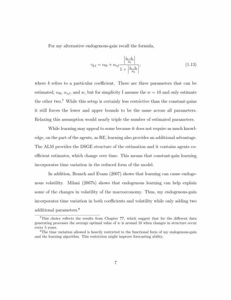
For my alternative endogenous-gain recall the formula,

γb,t = αlb + αsf

∣∣∣ bt−btσb

∣∣∣1 +

∣∣∣ bt−btσb

∣∣∣ , (1.13)

where b refers to a particular coefficient. There are three parameters that can be

estimated, αlb, αsf , and w, but for simplicity I assume the w = 10 and only estimate

the other two.7 While this setup is certainly less restrictive than the constant-gains

it still forces the lower and upper bounds to be the same across all parameters.

Relaxing this assumption would nearly triple the number of estimated parameters.

While learning may appeal to some because it does not require as much knowl-

edge, on the part of the agents, as RE, learning also provides an additional advantage.

The ALM provides the DSGE structure of the estimation and it contains agents co-

efficient estimates, which change over time. This means that constant-gain learning

incorporates time variation in the reduced form of the model.

In addition, Branch and Evans (2007) shows that learning can cause endoge-

nous volatility. Milani (2007b) shows that endogenous learning can help explain

some of the changes in volatility of the macroeconomy. Thus, my endogenous-gain

incorporates time variation in both coefficients and volatility while only adding two

additional parameters.8

7This choice reflects the results from Chapter ??, which suggest that for the different datagenerating processes the average optimal value of w is around 10 when changes in structure occurevery 5 years.

8The time variation allowed is heavily restricted to the functional form of my endogenous-gainand the learning algorithm. This restriction might improve forecasting ability.

7

2 Bayesian Estimation

In recent years there has been an abundance of papers that use Bayesian methods

to estimate DSGE models. An and Schorfheide (2007) provide general guidelines for

Bayesian estimation of DSGE models. Milani (2007a and 2007b) uses this technique

to estimate a model with learning similar to the one above. In contrast, Murray

(2008a, 2008b, and 2008c) all rely on a maximum likelihood approach. I favor the

Bayesian approach, because it provides clearer model comparison. Specifically, I use

a single block Random Walk Metropolis-Hastings (RW-MH) algorithm to sample the

posterior distribution of model parameters.

In order to conduct Bayesian estimation I rewrite the economy in state space

form:

ξt = Dt + Ftξt−1 +Gωt (2.1)

Yt = Hξt (2.2)

where ξt = (Zt, ut, gt, et, ιt)′, ωt ∼ N(0, Q), and Dt, Ft, G and H are the appropriate

matrices. Under RE Ft remains constant, since the deep parameters are constant,

and Dt = 0, since the RE solution has no intercept. Under learning, Dt contains

A−1(B + C)at−1 and zeros, and Ft contains A−1(Bct−1 + Cct−1F ), and updates the

unobservables.

Once in state space form, the procedure is straightforward. Let the vector Ω

8

contain the structural parameters of the model,

Ω = β, φ, λ, θπ, θx, µ, ρ, σg, σu, σe, σι, g. (2.3)

To form the posterior requires evaluating the likelihood function, L(•), at

the candidate parameter vector. The Kalman filter combined with the state space

described above produces the likelihood value. Multiplying the likelihood by the

priors, p(•) detailed below, results in the posterior distribution.

I use the Metropolis-Hastings algorithm to generate 1,250,000 draws from

the posterior distribution. The first 250,000 are discarded as burn-in values. The

Metropolis-Hastings algorithm relies on a high volume of draws from a candidate

distribution. These draws are accepted or rejected based on the ratio of the posterior

of the candidate to the previous draw.

Suppose that the previous draw is defined as Ω, and Ω∗ is defined as the can-

didate. A standard candidate distribution is a random walk through the parameter

space,

Ω∗ = Ω + cΣ, (2.4)

where c is a scaling term, and Σ is a covariance matrix. For certain algorithms

Σ = I for simplicity. I opt for simplicity, but modify some of the diagonal elements

to match the scale of the parameters.

In order to determine the acceptance probability, α, for each draw I use the

following equation,

α = min

p(Ω∗)L(Ω∗)

p(Ω)L(Ω), 1

. (2.5)

9

Thus if a candidate draw has a higher posterior value, then the previous draw the

algorithm accepts the candidate with probability 1. If the candidate has a much

lower posterior value, then the probability of acceptance is low. This ensures that

the algorithm ranges over some of the unlikely parameter values while fully exploring

the peak of the posterior.

Averaging the acceptance probabilities of each draw over all the draws results

in the acceptance rate. Geweke (1999) suggests calibrating the candidate distribution

to achieve acceptance rates between 25-40 percent.

2.1 Priors

Table 1 reports the prior distributions for each of the structural parameters in the

model. I use the analysis above to form the prior over the constant-gain. Similar

to Milani (2007b), I impose a dogmatic prior on β, namely, I set β equal to 0.99.

Gamma distributions form the priors for all the standard deviations and the slope

of the Phillips Curve. The monetary policy parameters have a normal prior, and the

correlation coefficients of the autocorrelated errors have uniform prior.

2.2 Data

The data come directly from the Federal Reserve Bank of St. Louis economic

database, FRED, and the Congressional Budget Office, CBO. The quarterly data

begin in 1984:III and ends in 2007:IV. I use the first twenty periods to initialize the

learning algorithm, thus the 1989:III-2007IV sample is used for the actual estimation.

Previous literature has shown that structural changes occurred prior to 1984, which

10

Table 1: Prior DistributionsDescription Param Distr. Stats. MeanDiscount Rate β – – 0.99Elas. of Subs. φ IG 1.5,1 1.5Slope of PC λ IG 0.25,1 0.25Feedback to Infl. θπ N 1.5,0.5 1.5Feedback to Output θx N 0.5,0.25 0.5Corr. of gt µ U 0,0.97 0.485Corr. of ut ρ U 0,0.97 0.485Std. gt σg IG 0.5,3 0.5Std. ut σu IG 0.5,3 0.5Std. et σe IG 0.5,3 0.5Std. ιt σι IG 0.5,3 0.5Gain Params γ U 0,0.4 0.2Alt. Params αlb,αsf U 0, 0.8 0.4Note: IG stands for Inverse-Gamma with scale and shape val-ues given, N stands for Normal with mean and variance valuesgiven, and U stands for Uniform with upper and lower boundvalues given.

would lead to further complexity of the model and estimation technique.9

I define inflation as the annualized quarterly rate of change of the GDP de-

flator. The output gap is the log difference between GDP and potential GDP (as

defined by the CBO). And finally, for the interest-rate I use the federal funds rate.

3 Results

Table 2 displays the results of estimations that differ in the assumptions over expec-

tations. I use three different criteria for model selection. Bayesian model compari-

son relies on obtaining the marginal likelihood. Chib and Jeliazkov (2001) provide

9For example see Fernndez-Villaverde and Rubio-Ramirez. (2007), Fernndez-Villaverde et al.(2009), Justiniano and Primiceri (2008), and Milani (2007).

11

Table 2: Estimation Results of a Model with Limited InformationDescription Param Pseudo-RE Constant-Gain Endog-GainElas. of Subs. φ 0.674 0.0344 0.0987Slope of PC λ 0.200 0.0986 0.238Feedback to Infl. θπ 1.134 1.0897 0.499Feedback to Output θx 0.0172 0.299 1.198Corr. of gt µ 0.945 0.789 0.469Corr. of ut ρ 0.954 0.722 0.823Std. gt σg 0.0932 0.968 0.843Std. ut σu 0.243 0.651 0.628Std. et σe 0.0985 0.133 0.1289Std. ιt σι 0.856 0.671 0.618Gain γ – 0.000698 –Lower Bound αlb – – 0.000349Scale Factor αsf – – 0.0496ML(CJ) -332.2 -303.9 -262.7ML(Harmonic) -300.7 -283.0 -264.2BIC 774.2 739.4 667.3Results presented here represent the mean of the posterior distribution of each pa-rameter. I calibrate the values of c to ensure acceptance rates between 25-40%. All ofthese estimations have the same starting values, except for the learning parameters.ML(CJ) is the marginal likelihood value calculated according to Chib and Jeliaskov(2001). ML(Harmonic) is the marginal likelihood using the modified harmonic mean,as suggested by Adolfson et al. (2007). BIC is calculated at the median value of theposterior distributions.

one method of approximation that relies on the same Markov Chain Monte Carlo

methodology used in sampling from the posterior. However, Adolfson et al. (2007)

suggest that in conjunction with RW-MH a modified harmonic mean reaches the

approximate marginal likelihood value more quickly. In addition, I use the Bayesian

Information Criterion (BIC).10 In each case numbers closer to zero indicate a better

model.

10In calculate the BIC I use the likelihood calculated at the median values of the posteriordistribution.

12

Looking at the estimates of the RE model the results seem consistent with

other literature. The data suggest that the model does not obey the Taylor rule, but

over this time period Fernndez-Villaverde et al. (2009) find similar results. However,

under learning these estimates get even smaller.

According to each of model comparison methods the data clearly favors the

learning models. Of the learning models the endogenous-gain version still provides

significant improvement even though only one additional parameter is estimated.

This comparison does not do the RE model justice, since under the learning assump-

tion the ALM coefficients vary over time.

A simple reduced form TVP would increase the number of parameters esti-

mated by five, which makes it unlikely to outperform a learning model. A preferred

model would allow the deep parameters to vary over time. Unfortunately, allowing

the combination of agents using the shocks as data and time varying deep parameters

seriously complicates the estimation. While the non-linearity in the reduced form

could be managed with a block sampling method, an estimation of the structural

equations would require non-linear techniques suggested by Fernndez-Villaverde, J.

and J. Rubio-Ramirez (2008). Therefore, I save this comparison for future work.

While the results from the RE model are consistent with previous research,

the data seem to favor the learning models. The estimation results from the learning

models, however, run counter to past empirical work.

Figure ?? displays the posterior distributions of each of the endogenous-gain

parameters. The data is clearly informative as the posterior distribution appear

quite different than the prior distributions. Some were so different that I chose not

13

to include representations of the prior distributions in these graphs.

Clearly the inter-temporal elasticity of substitution, the lower bound, and

the exogenous structural shocks clearly favor certain values of the distribution. The

other parameters have narrowed the prior distributions to a range of the parameter

space, but the data does not speak clearly for a particular value. The inter-temporal

elasticity of substitution is centered on 0.1, which is quite different than the prior.

The posterior of the lower bound parameter, which governs the lowest value that

the endogenous-gain can take, places a lot of weight near zero, which matches the

constant-gain estimation.

3.1 Expanding the Information Set

As noted earlier, the model above favors learning. By including information about

trend inflation in agents data set swings the favor toward rational expectations. The

estimation strategy remains the same, but the underlying matrices change.

I assume that agents observe the random walk time varying trend in much

the same way they observe the autocorrelated errors. This implies that agents know

the following,

υt = Fυt−1 + υt, (3.1)

14

where υt = (gt, ut, εt, ιt)′, υt are the respective iid errors, and

F =

ρg 0 0 0

0 ρu 0 0

0 0 0 0

0 0 0 1

.

Rewriting the NK model in a convenient form,

Zt = M0Et−1Zt +M1Et−1Zt+1 + Pυt, (3.2)

where M0 = A−1B, M1 = A−1C and

P = A−1

1 0 0 0

0 1 0 0

0 0 1 1

.

This change in formulation implies that the coefficient matrix in the MSV solution

is now a (3x4), the intercept terms, if any, remain the same.

Zt = (M0 +M1)at−1 + (M0ct−1 +M1ct−1F + PF )υt−1 + P υt. (3.3)

In contrast, the Law of Motion under rational expectations is,

Zt = cυt−1 + P υt, (3.4)

15

where c results from the vector, (I12 − (I4 ⊗M0 + F ′ ⊗M1))−1(F ′ ⊗ I3)vec(P ).

Table 3 presents similar results to when agents had less information. Both

learning models outperform the rational expectations model, and the endogenous-

gain model improves upon the constant-gain specification. In this case, the improve-

ment on rational expectations appears to be much greater.

The information used clearly has an effect on policy parameters. Assum-

ing RE, monetary policy followed the Taylor rule without the time varying trend

information, but did not with the information. Constant-gain learning obeyed the

Taylor rule in both scenarios, and endogenous-gain learning followed the Taylor

rule with the information.

In terms of comparing across the endogenous-gain specifications, I find that

the scale factor, αsf , doubles when agents incorporate the time varying trend in their

information set. This might result from agents using smaller time windows to follow

the random walk behavior of the trend.

One concern one might have is that some of the posterior means (specifically,

θπ, θx, σg, σu, σe and σι) remain close to the prior means. Figure 1 shows that this

is not the case. Only in one case does the mean of the prior did receive any weight

in the posterior distribution.

3.2 Perceptions vs. Reality

If one takes the learning hypothesis seriously then the learning estimation provides

a convenient by product, the agents’ perceptions. By backing out the PLM and the

ALM for the coefficients of the reduced form model that agents estimate, one can

16

Figure 1: Posterior Distributions of the Endogenous-Gain with Trend Information

17

Table 3: Estimation Results of a Model with Trend Interest-Rate InformationDescription Param RE Constant-Gain Endog-GainElas. of Subs. φ 0.456 1.0516 0.942Slope of PC λ 0.000144 0.0724 0.133Feedback to Infl. θπ 0.519 1.475 1.449Feedback to Output θx 0.612 0.482 0.465Corr. of gt µ 0.956 0.964 0.961Corr. of ut ρ 0.782 0.854 0.886Std. gt σg 0.454 0.616 0.558Std. ut σu 0.262 0.568 0.588Std. et σe 0.787 0.545 0.512Std. ιt σι 0.631 0.527 0.521Gain γ – 0.0000398 –Lower Bound αlb – – 0.000177Scale Factor αsf – – 0.0974ML(CJ) -350.4 -267.8 -256.2ML(Harmonic) -343.5 -342.9 -315.6BIC 827.5 701.7 674.0Results presented here represent the mean of the posterior distribution of eachparameter. I calibrate the values of c to ensure acceptance rates between 25-40%.All of these estimations have the same starting values, except for the learningparameters. ML(CJ) is the marginal likelihood value calculated according to Chiband Jeliaskov (2001). ML(Harmonic) is the marginal likelihood using the modifiedharmonic mean, as suggested by Adolfson et al. (2007). BIC is calculated at themedian value of the posterior distributions

interpret what agents react to, and how their reactions change over time. Since, in

terms of model comparison, the endogenous-gain estimation is preferred the analysis

below uses the results from the endogenous-gain learning estimation.

Figure 2 displays graphs of all twelve coefficients that agents estimate when

they do not have information on the trend of inflation. Each column represents each

equation for output, inflation and interest-rates respectively. The first row illustrates

the constant component of the forecasting equation, the following rows represent the

coefficients on the errors, gt,ut, and et, respectively. The black line in each graph

18

Figure 2: ALM (black line) and PLM (gray line) of Median Parameter Values withoutTrend Information

19

represents the ALM and the gray line the PLM.

Looking at the ALM I find evidence of structural breaks in four of the coeffi-

cients, which justifies the use of the endogenous-gain. The break in these four coeffi-

cients indicate that something the inflation process has changed. Though agents do

not follow the ALM very closely, they do react to the break. The structural break

occurs at the beginning of the new millennium, right before the 2001 recession.

This period also saw a change in perceptions about reactions to interest-rate

shocks. Prior to the break agents perceived that output and interest-rates responded

to past interest-rate shocks. After the break the perceived inflation responded the

most to past interest-rate shocks.

While agents, in general, do not perceive the ALM well, they do the worst

job following the intercept for inflation. Recall that I hypothesized that not allowing

agents to have trend interest-rate information would benefit the learning model.

This result shows that learning does not pick up the trend inflation as a part of the

intercept. This inability to track the trend of inflation probably causes the differences

between PLM and ALM.

Figure 3 displays the graphs of all 15 coefficients that agents estimate when

they do have information on the trend of inflation. The extra row supplies the

coefficients on the lagged trend of inflation.

In these graphs we see much less movement of the actual and perceived co-

efficients. There are still a few indications of a structural break around 2000, but

not nearly as significant as when agents use less information. In addition, agents do

much worse in following the ALM. It does not appear that the large gain in BIC

20

Figure 3: ALM (black line) and PLM (gray line) of Median Parameter Values withTrend Information

21

by learning results from time variation of the parameters, since coefficients exhibit

fairly stable dynamics.

4 Rational Expectations Data and Learning

One result in Milani (2007b) asserts that if agents are learning and there is no

conditional heteroscedasticity then an econometrician may be fooled into estimating

ARCH/GARCH models. However, no research to date has investigated the converse:

would a researcher observe learning dynamics when agents use rational expectations

(RE)?

Chevillon et al. (2010) investigate a similar question, but focus on identifica-

tion. They also use classical inference as opposed to the Bayesian techniques favored

here. Specifically, Chevillon et al. show that the Anderson-Rubin statistic, with

appropriate choice of instruments, can result in valid inference.11

The economy is described by a similar NK model as above except I remove

the time varying trend of the interest-rate from equation (??).

it = θππet + θxx

et + εt, (4.1)

In order to derive the rational expectations solution used for the simulations

I rewrite the NK model in matrix notation,

yt = M0yet +M1y

et+1 + Pυt, (4.2)

11Appropriate instruments usually are predetermined variables.

22

where yt = (xt, πt, it)′, υt = (gt, ut, εt)

′, and M0, M1, and P are the appropriate

matrices. Assuming the MSV solution yREt = cυt−1 one can substitute in and solve

for the RE coefficients c. The substitution yields,

c = (M0c+M1cF + PF ). (4.3)

Using the following identity vec(ABC) = (C ′ ⊗ A)vec(B), one can easily show that

c results from the vector, (I9 − (I3 ⊗M0 + F ′ ⊗M1))−1(F ′ ⊗ I3)vec(P ). Thus, the

RE law of motion is,

yt = cυt−1 + P υt. (4.4)

For the learning estimation procedure I follow the same steps as above to

obtain the following ALM:

Zt = A−1(B + C)at−1 + A−1(Bct−1 + Cct−1F )Fυt−1 + A−1υt. (4.5)

4.1 Monte Carlo Experiment

For simulations of the rational expectations model I use the same values for the NK

parameters as the previous chapter. Finally, I calibrate the parameters of the error

terms as µ = ρ = 0.8 and σg = σu = σe = 0.2. I conduct 100 simulations of RE data

of 120 periods each. This means that each estimation relies on 100 periods of data.

In order to make an accurate portrayal I estimate the model assuming rational

expectations and assuming learning. Table 4 displays the results for the Monte Carlo

experiment.

23

Table 4: RE and Learning Monte Carlo Experiment Results

Description Param Actual RE-Est Learning-EstElas. of Subs. φ 6.369 6.355 6.425

(0.210) 0.243(0.252) (0.335)

Slope of PC λ 0.024 0.0234 0.022(0.0050) (0.0037)(0.0060) (0.0002)

Feedback to Infl. θπ 1.5 1.810 1.130(0.333) (0.0752)(0.358) (0.0628)

Feedback to Output θx 0.5 0.736 0.252(0.253) (0.0574)(0.267) (0.0348)

Corr. of gt µ 0.8 0.799 0.783(0.0064) (0.0169)(0.0073) (0.0032)

Corr. of ut ρ 0.8 0.793 0.852(0.0580) (0.0450)(0.0521) (0.0109)

Std. gt σg 0.2 0.206 0.253( 0.0170) (0.0257)(0.0174) (0.0065)

Std. ut σu 0.2 0.201 0.467(0.0163) (0.0637)(0.0157) (0.0710)

Std. et σe 0.2 0.201 0.243(0.0149) (0.0217)(0.0150) (0.0095)

Constant-Gain γ 0.010(0.0033)(0.0001)

ML(CJ) -146.1 -286.2ML(Harmonic) -46.3 -118.5BIC 372.1 662.5Note: Results presented here represent the mean of each parameter. Regularparentheses indicate average standard deviation within estimations. Itali-cized parentheses indicate standard deviation across estimations. ML(CJ)is the marginal likelihood value calculated according to Chib and Jeliaskov(2001). ML(Harmonic) is the marginal likelihood using the modified har-monic mean, as suggested by Adolfson et al. (2007). BIC is calculated atthe median value of the posterior distributions

24

The RE estimation naturally pins down all the parameter estimates within a

single standard deviations. This holds within each estimation and across the esti-

mations. The learning model, however, has small standard errors within each esti-

mation, and relatively large standard errors across estimations. This suggests that

particular realizations of the rational expectations model can fool a researcher into

believing that learning exists in the model. Not surprisingly, the model comparison

values overwhelmingly favor the rational expectations model.

Turning to the parameter estimates of learning estimation a striking pattern

emerges. The learning assumption cause the researcher to underestimate the deep

parameters and the correlations and overestimate the standard errors of the shocks.

The learning process subsumes some of the autocorrelation, and as a byproduct it

alters the parameter estimates.

Another interesting point is that the learning estimation does not nest the

rational expectations solution like one might suspect. In the theoretical learning

literature an extremely small constant-gain is typically considered consistent with

rational expectations. Even though the constant-gain term is not statistically differ-

ent from zero, all the parameter estimates of the learning estimation do not contain

the actual parameter values in a 95% confidence interval.

5 Conclusion

Using a simple NK model I show that endogenous-gain learning provides significant

improvement on both RE and constant-gain learning. I use a different approach than

other DSGE estimations by using the lagged, filtered estimates of the residuals as

25

the regressors. I find that, conditional on the specification, agents perceptions do

not align with the actual path of the reduced form coefficients.

One reason why learning might fit the data better than RE is because it allows

for time-variation in the reduced form coefficients, however, analysis of the reduced

form coefficients shows little variation over time. In addition, I have shown that if the

underlying data generating process resulted from RE learning would perform poorly.

The Monte Carlo experiment also underscores that a learning estimation does not

nest the rational expectations result. Further research is necessary to determine why

this is the case.

26

Bibliography

[1] Beck, G.W. and V. Wieland. “Learning and Control in a Changing EconomicEnvironment,” Journal of Economic Dynamics and Control 26.9-10 (2002):1359-1377

[2] Blume, L. and M. Bray and D. Easley. “Introduction to the Stability of RationalExpectations Equilibrium.,” Journal of Economic Theory 26.2 (1982):313-317

[3] Bray, M. “Learning, Estimation, and the Stability of Rational Expectations,”Journal of Economic Theory 26.2 (1982):318-339

[4] Bray, M. and N.E. Savin. “Rational Expectations Equilibria, Learning andModel Specification.,” Econometrica 54.5 (1986):1129-1160

[5] Bullard, J. “Time-Varying Parameters and Non-Convergence to Rational Ex-pectations Under Least Square Learning,” Economic Letters 40.2 (1992):159-166

[6] Carceles-Poveda, E. and C. Giannitsarou. “Adaptive Learning in Practice,”Journal of Economic Dynamics and Control 31.8 (2007):2659-2697

[7] Evans, G. “Expectational Stability and the Multiple Equilibria Problem inLinear Rational Expectations Models,” Quarterly Journal of Economics 100.4(1985):1217-1233

[8] Evans, G.W. and S. Honkapohja. “Economic Dynamics With Learning: NewStability Results,” Review of Economic Studies (1998):23-44

[9] ——. “Monetary Policy, Expectations and Commitment,” The ScandinavianJournal of Economics 108.1 (2006):15-38

[10] ——. “Robust Learning Stability With Operational Monetary Policy Rules,”forthcoming (2008)

[11] Frydman, R. “Towards an Understanding of Market Processes: Individual Ex-pectations, Learning, and Convergence to Rational Expectations Equilibrium,”The American Economic Review 72.4 (1982):652-668

27

[12] Marcet, A. and J.P. Nicolini. “Recurrent Hyperinflations and Learning,” Amer-ican Economic Review 93.5 (2003):1476-1498

[13] McGough, B. “Statistical Learning With Time-Varying Parameters,” Macroe-conomic Dynamics 7.01 (2003):119-139

[14] Milani, F. “Learning and Time-Varying Macroeconomic Volatility,” Manuscript,UC-Irvine (2007)

[15] ——. “Expectations, Learning and Macroeconomic Persistence,” Journal ofMonetary Economics 54.7 (2007):2065-2082

[16] Muth, J. “Rational Expectations and the Theory of Price Movements,” Econo-metrica 29.3 (1961):315-335

[17] Wieland, V. “Monetary Policy, Parameter Uncertainty and Optimal Learning,”Journal of Monetary Economics 46 (2000):199-228

[18] Woodford, M. Interest and Prices: Foundations of a Theory of Monetary Policy.Princeton University Press, 2003.

28