W ()).)(# - W / ,& (- W ' !#(! W) W #*)& , W '#.. ,- Wlib.tkk.fi/Diss/2012/isbn9789526048697/isbn9789526048697.pdf · Abstract Aalto University, P.O. Box 11000, FI-00076 Aalto Author

9HSTFMG*aeigia+

Electrom

agnetic Nanophotonics:

Superlens Imaging of D

ipolar Em

itters and Cloaking in W

eak Scattering

Aalto University publication series DOCTORAL DISSERTATIONS 151/2012

Electromagnetic Nanophotonics: Superlens Imaging of Dipolar Emitters and Cloaking in Weak Scattering

Timo Hakkarainen

A doctoral dissertation completed for the degree of Doctor of Science in Technology to be defended, with the permission of the Aalto University School of Science, at a public examination held in Auditorium F239a of the F building (Otakaari 3, Espoo, Finland) on the 30th of November 2012 at 12 noon.

Aalto University School of Science Department of Applied Physics Optics and Photonics

Supervising professor Professor Ari T. Friberg Thesis advisor Docent Tero Setälä Preliminary examiners Professor Martti Kauranen Tampere University of Technology, Finland Professor Karl-Heinz Brenner University of Heidelberg, Germany Opponent Professor Micheal A. Fiddy University of North Carolina, USA

Aalto University publication series DOCTORAL DISSERTATIONS 151/2012 © Timo Hakkarainen ISBN 978-952-60-4868-0 (printed) ISBN 978-952-60-4869-7 (pdf) ISSN-L 1799-4934 ISSN 1799-4934 (printed) ISSN 1799-4942 (pdf) http://urn.fi/URN:ISBN:978-952-60-4869-7 Unigrafia Oy Helsinki 2012 Finland Publication orders (printed book): [email protected]

Abstract Aalto University, P.O. Box 11000, FI-00076 Aalto www.aalto.fi

Author Timo Hakkarainen Name of the doctoral dissertation Electromagnetic Nanophotonics: Superlens Imaging of Dipolar Emitters and Cloaking in Weak Scattering Publisher School of Science Unit Department of Applied Physics

Series Aalto University publication series DOCTORAL DISSERTATIONS 151/2012

Field of research Engineering Physics, Physics

Manuscript submitted 21 August 2012 Date of the defence 30 November 2012

Permission to publish granted (date) 29 October 2012 Language English

Monograph Article dissertation (summary + original articles)

Abstract Two novel topics of nanophotonics, near-field imaging by superlenses and invisibility cloakingwith slab scatterers, are investigated within the context of classical electromagnetic theory.

In superlens imaging the objects are radiating point dipoles or externally excited dipo-lar emitters. The imaging element is a metallic or a slightly lossy negative-index material(NIM) slab with thickness of a few tens of nanometers. The electromagnetic angular spectrumrepresentation is used to derive the Green tensors for the slab’s transmission and reflection.With this formalism the point-spread function of the imaging system is numerically evalu-ated, which enables one to assess resolution and image brightness. The dependence of imagequality on the system parameters, dipole orientations, and near-field interactions among theobjects and the lens is investigated.

It is shown that both metallic and lossy metamaterial superlenses allow for image defini-tions beyond the usual diffraction limit of half the wavelength λ. High image quality requiresa low-absorption slab and a good impedance match of the lens and its surroundings. In theimmediate vicinity of the slab the dipole-slab interaction prevents the dipole from radiating.With low-loss NIM the interaction is weak and of short range. For silver slabs the interactionis stronger and reaches over the near-field zone, adversely influencing the imaging capabili-ties. With two dipole-like objects the emission is also suppressed by dipole-dipole near-fieldinteractions, in particular with molecular objects while the effect is weak for glass or metallicnanoparticles. Due to interference subwavelength definition can only be attained for dipolesaligned predominantly orthogonal to the slab. Such a situation is achieved with excitationby total internal reflection. In optimal circumstances, resolutions of about λ/5 for silver andλ/10 for metamaterial lens are reached in three-dimensional configurations.

Invisibility cloaking is considered within weak optical scattering in slab geometry. Theconditions for cloaking in forward and backward directions are established, enabling the de-termination of the cloak’s refractive-index distribution for stratified objects. For any absorbingobject forward cloaking is achieved with a lossy NIM or gainy ordinary-material slab. Thecloaking is perfect for incident fields of any spatial structure and bandwidth. Backward cloak-ing is found possible with self-imaging fields. In both cases the cloak’s dispersive propertiesresemble those of the object.

Keywords near-field optics, superlens imaging, optical scattering

ISBN (printed) 978-952-60-4868-0 ISBN (pdf) 978-952-60-4869-7

ISSN-L 1799-4934 ISSN (printed) 1799-4934 ISSN (pdf) 1799-4942

Location of publisher Espoo Location of printing Helsinki Year 2012

Pages 140 urn http://urn.fi/URN:ISBN:978-952-60-4869-7

Tiivistelmä Aalto-yliopisto, PL 11000, 00076 Aalto www.aalto.fi

Tekijä Timo Hakkarainen Väitöskirjan nimi Sähkömagneettinen nanofotoniikka: dipolilähteiden kuvaaminen superlinsseillä ja heikosti sirottavien kohteiden häivyttäminen Julkaisija Perustieteiden korkeakoulu Yksikkö Teknillisen fysiikan laitos

Sarja Aalto University publication series DOCTORAL DISSERTATIONS 151/2012

Tutkimusala Teknillinen fysiikka, fysiikka

Käsikirjoituksen pvm 21.08.2012 Väitöspäivä 30.11.2012

Julkaisuluvan myöntämispäivä 29.10.2012 Kieli Englanti

Monografia Yhdistelmäväitöskirja (yhteenveto-osa + erillisartikkelit)

Tiivistelmä Tyossa tutkitaan klassista sahkomagneettista teoriaa kayttaen kahta modernin nanofotoniikanaihetta: lahikenttakuvaamista superlinsseilla ja kohteen haivyttamista.

Superlinsseilla kuvattaessa objektina toimii sateileva pistedipoli tai dipolimainen sirot-taja. Kuvauslinssina kaytetaan metallista tai haviollisesta metamateriaalista koostuvaa levya,jonka paksuus on kymmenien nanometrien suuruusluokkaa. Tyossa johdetaan Greenin ten-sorit levyn lapaisylle ja heijastukselle sahkomagneettisen kulmaspektriesityksen avulla. Tallaformalismilla lasketaan numeerisesti dipolin kuvajakauma, mika mahdollistaa kuvan kirkkau-den ja tarkkuuden maarittamisen. Tarkasteltavana on syntyneen kuvan laadun riippuvuus ku-vaussysteemin parametreista, objektidipolien suunnasta seka objektien ja linssin valisista la-hikenttavuorovaikutuksista.

Tyossa osoitetaan, etta puolen aallonpituuden (λ) kuvaustarkkuus voidaan ylittaa metalli-ja metamateriaalisuperlinsseilla. Terava kuva edellyttaa pienihavioista kuvauselementtia sekahyvaa impedanssien sovitusta elementin ja ympariston valilla. Linssin valittomassa laheisyy-dessa objekti-linssi -vuorovaikutukset heikentavat dipolilahteen sateilyn voimakkuutta. Meta-materiaalilinssille ilmio on heikko, mutta metallilinssin tapauksessa se on merkittava ja kattaalahikenttaalueen heikentaen elementin kuvausominaisuuksia. Myos kahden molekyylimaisenobjektin vuorovaikutukset vahentavat emissiota, kun taas lasi- ja metallinanohiukkasia ku-vattaessa nain ei kay. Interferenssin johdosta alle puolen aallonpituuden kuvaustarkkuussaavutetaan vain, jos dipolit osoittavat kohtisuoraan kuvauslevya kohti. Tama saadaan aikaanvirittamalla dipolit kokonaisheijastuksella luodulla vaimenevalla kentalla. Optimaalisessatilanteessa kolmidimensioisella kuvaussysteemilla paastaan kuvaustarkkuuteen, joka on noinλ/5 metallilinssille ja λ/10 metamateriaalilinssille.

Tyossa tarkastellaan heikosti valoa sirottavien objektien haivyttamista levygeometriassa.Ilmiolle maaritetaan tarkastelusuunnasta riippuvat ehdot, jotka mahdollistavat haivemateri-aalin taitekertoimen laskemisen. Kerrosrakenteinen objekti voidaan saattaa edestapain naky-mattomaksi haviollisella metamateriaalilla tai vahvistavalla aineella. Haivyttaminen on taydel-lista ja toteutuu mielivaltaiselle valaistukselle. Myos heijastuksessa objektin nakymattomaksitekeminen on mahdollista, mutta vain itsekuvautuvien kenttien tapauksessa. Haivemateriaalindispersiiviset ominaisuudet maaraytyvat objektin vastaavista ominaisuuksista.

Avainsanat lähikenttäoptiikka, superlinssikuvaus, optinen sironta

ISBN (painettu) 978-952-60-4868-0 ISBN (pdf) 978-952-60-4869-7

ISSN-L 1799-4934 ISSN (painettu) 1799-4934 ISSN (pdf) 1799-4942

Julkaisupaikka Espoo Painopaikka Helsinki Vuosi 2012

Sivumäärä 140 urn http://urn.fi/URN:ISBN:978-952-60-4869-7

Preface

In my first grade of the elementary school I remember feeling frustrated in

maths class when we were told to color three apples out of five. I asked the

teacher to give me a more difficult problem to solve. I do not remember the

formulation of this highly demanding task she gave me but I remember

the solution. It was 18.

Eighteen years later, in 2008, I started my PhD studies, now with more

questions than solutions. My four-year research is summarized in this

dissertation, and it has been carried out in the Department of Applied

Physics of Aalto University School of Science. Now, I want to take this

opportunity to thank some people for their support during the project.

I am most indebted to my supervisor Professor Ari T. Friberg. Your

persistent support and knowledge on electromagnetics has been an indis-

pensable advantage. I have learned from you a great deal about optics,

research work in general, and of leadership. Your endless enthusiasm

towards research projects and your way to challenge students’ thinking

inspire the rest of Theory Group. I am also very grateful to my instructor,

Docent Tero Setälä, for his guidance along the way and for believing in my

ability to complete this thesis. Further, I thank Professor Matti Kaivola

for the opportunity to work in the department.

During the course of this work I have had the pleasure to collaborate

with many talented people in the Optics and Photonics Group. I wish

to thank Dr. Markus Hautakorpi, Dr. Klas Lindfors, and Doc. Andriy

Shevchenko for insightful discussions on optics. I am also grateful to

M.Sc. Henri Kellock, M.Sc. Kimmo Kokkonen, M.Sc. Lauri Lipiäinen,

Dr. Esa Räikkönen, M.Sc. Timo Voipio, and Orvokki Nyberg for many

valuable advice in practical matters. Special thanks go to my workmates,

M.Sc. Andreas Norrman and Dr. Arri Priimägi, who have had positive

influence on my well-being with common interests also beyond optics.

i

Preface

I am also fortunate to have many important friends who, each in their

unique way, have supported me during this work. First, I wish to express

my gratitude for two of them, M.Sc. Teemu Hakkarainen and M.Sc. Juha

Pirkkalainen, who are talented physicists and with whom I have shared

invaluable thoughts during our paths in university studies. I also want

to thank a bunch of inspiring and sparkling people, Anna, Anssi, Elina,

Ilmari, Jani, Jere, Juho, Jukka, Kaisa, Lasse, Lauri K., Mari H., Mari

K., Pälvi, and Tero K. You all have enriched my life with performing arts,

music, traveling, wandering in nature, thoughtful conversations, and with

a couple of obscure dusk-till-dawn adventures.

I wish to acknowledge the Finnish Graduate School of Modern Optics

and Photonics and the Academy of Finland for funding my doctoral re-

search. In addition, personal grants from the Finnish Foundation for

Technology Promotion and Emil Aaltonen Foundation are gratefully ap-

preciated.

I am deeply grateful to my dear parents and sisters for their constant

support and encouragement throughout my life. Most of all, I would like

to thank Marjo, my lovely, little creature and companion in life, for her

endless patience and love during this work.

Helsinki, October 31, 2012,

Timo Hakkarainen

ii

Contents

Preface i

Contents iii

List of Publications v

Author’s Contribution vii

1. Introduction 1

2. Electric point dipole 5

2.1 Point-dipole radiation . . . . . . . . . . . . . . . . . . . . . . . 5

2.2 Effective polarizability of a dipolar emitter . . . . . . . . . . 6

2.3 Polarizability of a small particle . . . . . . . . . . . . . . . . . 7

2.4 Coupled dipole method . . . . . . . . . . . . . . . . . . . . . . 8

3. Electric field of a point dipole in a three-layer structure 11

3.1 Angular spectrum representation of dipole field . . . . . . . 11

3.2 Reflection and transmission coefficients

for a three-layer structure . . . . . . . . . . . . . . . . . . . . 13

3.2.1 Boundary condition method . . . . . . . . . . . . . . . 13

3.2.2 Partial-wave summation method . . . . . . . . . . . . 14

3.3 Green’s tensors for reflection and transmission . . . . . . . . 15

4. Optical properties of superlens materials 17

4.1 Metals . . . . . . . . . . . . . . . . . . . . . . . . . . . . . . . . 17

4.1.1 Electromagnetic response of metals . . . . . . . . . . 17

4.1.2 Surface plasmons . . . . . . . . . . . . . . . . . . . . . 18

4.2 Metamaterials . . . . . . . . . . . . . . . . . . . . . . . . . . 20

4.2.1 Material parameters of metamaterials . . . . . . . . . 20

4.2.2 Structure and progress of metamaterial designs . . . 21

iii

Contents

4.2.3 Electromagnetic properties of NIMs . . . . . . . . . . 22

4.2.4 Applications of metamaterials . . . . . . . . . . . . . . 24

5. Near-field imaging with slab superlenses 25

5.1 Resolution in far-field imaging . . . . . . . . . . . . . . . . . . 25

5.1.1 Point-spread function . . . . . . . . . . . . . . . . . . . 25

5.1.2 Diffraction limit . . . . . . . . . . . . . . . . . . . . . . 27

5.2 The perfect lens . . . . . . . . . . . . . . . . . . . . . . . . . . 28

5.2.1 Focusing of propagating waves . . . . . . . . . . . . . 28

5.2.2 Enhancement of evanescent waves . . . . . . . . . . . 30

5.3 Imaging with superlenses . . . . . . . . . . . . . . . . . . . . 31

5.3.1 Enhancement of evanescent waves . . . . . . . . . . . 31

5.3.2 Development of near-field superlenses . . . . . . . . . 32

5.4 Near-field imaging of point-like objects with superlenses . . 34

5.4.1 Imaging of a radiating dipole with NIM superlens . . 34

5.4.2 Imaging of a radiating dipole with silver superlens . 35

5.4.3 Imaging of a dipole interacting with superlens . . . . 36

5.4.4 Imaging of two interacting dipoles . . . . . . . . . . . 38

6. Optical cloaking 41

6.1 Survey of optical cloaking . . . . . . . . . . . . . . . . . . . . 41

6.2 Optical scattering theory . . . . . . . . . . . . . . . . . . . . . 43

6.3 Cloaking in the Born approximation . . . . . . . . . . . . . . 45

7. Conclusions and outlook 47

Appendix A: Basic tools of electromagnetic optics 49

A.1 Maxwell’s equations . . . . . . . . . . . . . . . . . . . . . . . . 49

A.2 Response of matter to electromagnetic fields . . . . . . . . . . 50

A.3 Wave equations . . . . . . . . . . . . . . . . . . . . . . . . . . . 51

A.4 The Green function . . . . . . . . . . . . . . . . . . . . . . . . . 51

A.5 Monochromatic field . . . . . . . . . . . . . . . . . . . . . . . . 52

A.6 Angular spectrum representation . . . . . . . . . . . . . . . . 53

A.7 Boundary conditions . . . . . . . . . . . . . . . . . . . . . . . . 55

A.8 Fresnel’s coefficients . . . . . . . . . . . . . . . . . . . . . . . . 56

References 57

Errata 71

Publications 73

iv

List of Publications

This thesis consists of an overview and of the following publications which

are referred to in the text by their Roman numerals.

I Timo Hakkarainen, Tero Setälä, and Ari T. Friberg. Subwavelength

electromagnetic near-field imaging of point dipole with metamaterial

nanoslab. Journal of the Optical Society of America A 26, 10, 2226–

2234, September 2009.

II Timo Hakkarainen, Tero Setälä, and Ari T. Friberg. Near-field imaging

of point dipole with silver superlens. Applied Physics B 101, 4, 731–734,

July 2010.

III Timo Hakkarainen, Tero Setälä, and Ari T. Friberg. Electromagnetic

near-field interactions of a dipolar emitter with metal and metamaterial

nanoslabs. Physical Review A 84, 3, 033849, September 2011.

IV Timo Hakkarainen, Tero Setälä, and Ari T. Friberg. Near-field imag-

ing of interacting nano objects with metal and metamaterial superlenses.

New Journal of Physics 14, 043019, April 2012.

V Tero Setälä, Timo Hakkarainen, Ari T. Friberg, and Bernhard J. Hoen-

ders. Object-dependent cloaking in the first-order Born approximation.

Physical Review A 82, 1, 013814, July 2010.

v

List of Publications

vi

Author’s Contribution

The author has had a key role in all aspects of the research work summa-

rized in this thesis and reported in Publications I–V.

Publications I–IV

The author has performed all the analytical calculations, as well as the

numerical implementations. The author has had a major role in the in-

terpretation of the results, and he has written the first versions of the

manuscripts.

Publication V

The author has strongly contributed to the analytical and numerical cal-

culations. He has participated in the interpretation of the results and in

writing the manuscript.

Another publication to which the author has contributed:

A. Hakola, T. Hakkarainen, R. Tommila, and T. Kajava. Energetic Bessel-

Gauss pulses from diode-pumped solid-state lasers. Journal of the Optical

Society of America B 27, 11, 2342–2349, November 2010.

In addition to the publications in peer-reviewed journals, the author has

presented the research summarized in the thesis in several national and

international1 conferences.

1

EOS Annual Meeting, Paris, 2008;

4th EOS Topical Meeting on Advanced Imaging Techniques, Jena, 2009;

3rd Congress on Advanced Electromagnetic Materials in Microwaves and Optics, London, 2009;

META’10, 2nd Conference on Metamaterials, Photonic Crystals and Plasmonics, Cairo, 2010;

4th Congress on Advanced Electromagnetic Materials in Microwaves and Optics, Karlsruhe, 2010;

Biomedical Optics, Miami, 2012

vii

Author’s Contribution

viii

1. Introduction

The current knowledge to tailor material properties has enabled the gen-

eration of novel photonic media with artificially engineered nano-scale

structures. These materials are known as metamaterials and they ex-

hibit optical properties not found in natural media [1–3]. Especially in

the microwave regime but recently also at optical frequencies, metamate-

rials have brought a diverse amount of engrossing physics and potential

applications into the focus of scientists [4–6]. In particular, the possibility

of near-field superlenses providing subwavelength image definition would

have significant applications in several fields of technology and science,

e.g., optical nano-scale microscopy and biosensing, ultra-accurate optical

lithography, and data storage [7]. Another interesting topic born with

the metamaterials is optical cloaking: an object is made invisible or less

detectable to observer by covering it with a proper material [8, 9]. The

theoretical work of my thesis arose from the interest of the Optics and

Photonics Group at Aalto University School of Science on these two novel

and challenging research fields. The work may be seen as a natural ex-

tension for the group’s long experience to apply classical electromagnetic

theory to research problems of nanophotonics.

The resolution in conventional (far-field) optical imaging is limited by

the wavelength of light (λ) and the numerical aperture (NA) of the system

[10]. However, optical imaging beyond the classic Rayleigh–Abbe diffrac-

tion limit of λ/2 in spatial resolution has long been a subject of interest

to scientists [10, 11]. This limit emerges because the information on the

finest features of the object is carried by the high-spatial-frequency waves,

known as evanescent waves, which decay exponentially. So, not even the

best of the far-field lenses can collect the evanescent waves in the image.

The advent of near-field optics has brought out various methods that al-

low one to catch the evanescent modes and the associated subwavelength

1

Introduction

information [10–12]. A widely employed approach in nanophotonics is op-

tical near-field microscopy, which makes use of scanning local probes and

near-field imaging elements [12]. In these techniques the imaging device

is placed at a subwavelength distance from the object, enabling detection

of the evanescent field created by the object and thereby increasing the

effective NA.

During the past ten years, near-field imaging with metallic and meta-

material superlenses has inspired an increasing number of works [7] fol-

lowing the suggestion of the ‘perfect lens’ [13]. The perfect lens (in air) is

a lossless nanoslab having its relative electric permittivity and magnetic

permeability equal to −1. It is an idealized case of negative-index mate-

rials (NIMs) that are characterized by negative refractive index. Such a

lens cancels the phase changes accumulated by propagating waves and

restores the evanescent wave contributions, and thus delivers an undis-

torted image with unlimited definition. However, any realistic metamate-

rial is necessarily lossy leading to absorption of the object radiation and to

interactions between the lens and the object which degrades image resolu-

tion. Lenses that take the practical limitations into account, and yet allow

resolution well beyond the wavelength of the light (deep-subwavelength

resolution), are known as superlenses. Despite the rapid progress on

metamaterials, experimental NIM-lens realizations are few [6, 7]. Be-

sides NIM lenses, subwavelength imaging can be achieved with metallic

nanoslabs exhibiting plasmon resonances [7, 13]. The first experimen-

tal demonstrations of silver superlenses with subwavelength resolution

(about λ/6) were reported in 2005 [14, 15]. Recently an improved silver-

lens design, providing λ/12 resolution in imaging of a two-dimensional

grating object, was fabricated [16].

To make things invisible has always attracted people. The invention of

metamaterials has brought this dream from science fiction closer to daily

life [8, 9]. In 2006, it was found that an artificial medium having spa-

tially changing optical properties could bend light in extraordinary man-

ners. One example of this is an optical cloak which guides light around

an object, similarly to the flow of water around a stone, making the object

invisible or less detectable. The possibility to design artificial cloaking

materials relies on a variety of mathematical techniques, the best known

of which is transformation optics [17, 18]. The breakthrough in cloaking

launched what can safely be called a boom among the scientists: the first

cloaking device operating at microwave frequencies was realized shortly

2

Introduction

after the invention of cloaking [19], and theoretical researches on new ge-

ometries pushing the concept towards the optical frequencies have been

published at an accelerating rate [8,9]. The early cloaking schemes suffer

from high losses and narrow operation bandwidth, but new designs have

enabled low-loss and broad-band optical cloaks [20–22]. Striking propos-

als of space-time electromagnetic cloaks, concealing not just objects in

space but also events in time, have recently been put forward [23,24].

The major part of this thesis concentrates on near-field imaging with

metallic and metamaterial superlenses. We consider dipolar objects cre-

ating electric fields with three orthogonal components that are imaged

by planar slab lenses in three dimensions. Our main aim is to find out

the optimal conditions for the imaging in terms of resolution and bright-

ness. In Publications I–IV we develop a detailed theoretical formalism for

this purpose and show how the system geometry, material properties, and

dipole orientations influence the imaging. Further, the near-field interac-

tions among the objects and the imaging element are taken into account

and their effects on the image quality are assessed. Our work constitutes

fundamental research; the results aid in the development of superlenses

and also facilitate in designing superlens imaging setups. A minor topic

of this thesis is optical cloaking. In Publication V we consider cloaking

from a new perspective: using optical scattering theory we study weakly

scattering stratified objects and show that they can be cloaked by suitable

slab structures.

The main points of this thesis are to assess the resolution of superlenses,

as defined by dipolar point objects, and to evaluate the effects of dipole

interactions on near-field imaging. Therefore I begin by introducing in

Chapter 2 the theory of electric point dipoles, which I also use to describe

nanoscale scatterers. Chapter 3 then contains the methods for evaluating

the dipole field on both sides of the slab structures. In Chapter 4, I discuss

the optical properties of metals and metamaterials, and give a review on

the progress on metamaterials. Chapter 5 contains the theoretical back-

ground and recalls the development of the near-field superlenses. This

chapter also includes a summary of our research on the near-field imag-

ing with superlenses that is reported in Publications I–IV. Since optical

cloaking is a secondary topic of this thesis I discuss it separately after su-

perlens imaging. More specifically, in Chapter 6 I first give an overview of

cloaking with various methods including transformation optics. Then I in-

troduce the elements of electromagnetic scattering theory, and summarize

3

Introduction

our work on cloaking with weak scatterers that is reported in Publication

V. The main conclusions and future prospects of superlens imaging and

cloaking are discussed in Chapter 7. The Maxwell equations, the basic

theory of electromagnetic optics, and the main mathematical tools that

we use are outlined in Appendix A.

4

2. Electric point dipole

In classical electromagnetic optics small scatterers, such as atoms, molecu-

les, or nanoparticles, are often treated as electric point dipoles [10,12]. In

Publications I–IV we study the near-field imaging of dipole-like nanoob-

jects with metallic and metamaterial superlenses. This chapter intro-

duces how the characteristic properties of dipolar emitters, e.g., dipole

moment, polarizability, and electric field, can be calculated.

2.1 Point-dipole radiation

The electromagnetic field generated by a point dipole is conventionally

deduced using the theory of Green’s functions as described in App. A.4. In

a linear, isotropic, stationary, homogeneous, and spatially nondispersive

medium the electric field at a point r generated by an arbitrarily oriented

dipole, having the dipole moment q and located at r0, takes the form [10]

E(r, ω) = μω2↔G(r, r0, ω)q, (2.1)

where μ denotes the magnetic permeability of the medium and ω is the

angular frequency. The Green function,↔G(r, r0, ω), is a second-rank tensor

and the dipole moment is a vector quantity with Cartesian components qx,

qy, and qz. The dyadic, outgoing (time-dependence e−iωt), free-space Green

function has an expression [10,25]

↔G(r, r0, ω) =

[↔I+

1k2∇∇

]G(r, r0, ω), (2.2)

where↔I is the unit dyad, k is the wave number, and G(r, r0, ω) denotes the

scalar free-space Green function [10,25]

G(r, r0, ω) =eik|r−r0|

4π|r− r0| . (2.3)

5

Electric point dipole

Inserting the scalar Green function into Eq. (2.2), one finds the Green

tensor in the Cartesian system [10]

↔G(r, r0, ω) =

[(1 +

ikR

− 1k2R2

)↔I+

(− 1− 3i

kR+

3k2R2

)RRR2

]eikR

4πR, (2.4)

where R = |R| = |r− r0| and RR denotes the vector outer product.

The Green tensor in Eq. (2.4) defines a symmetric 3 × 3 matrix which,

together with Eq. (2.1), specifies the electric field of an electric dipole. The

Green tensor contains three different terms according to its R dependence.

In the far field, for which R � λ, only the terms with (kR)−1 survive. On

the other hand, in the near field (R � λ) the terms with (kR)−3 give the

major contribution, whereas the intermediate field (R ≈ λ) is dominated

by the terms with (kR)−2.

2.2 Effective polarizability of a dipolar emitter

An effective polarizability is often introduced to take into account the in-

teraction of a single dipolar particle with its environment. The interaction

results from the fact that the emitted dipole field scatters back from the

inhomogeneities of the environment and influences the dipole properties.

The dipole moment of a polarizable particle located at r = r0 is related to

the total exciting field Eex,tot at the dipole site as [10]

q =↔α(ω)Eex,tot(r0, ω), (2.5)

where↔α is the polarizability tensor of the emitter. The field Eex,tot can be

divided into two contributions:

Eex,tot(r0, ω) = Eex(r0, ω) + Eds(r0, ω), (2.6)

with Eex being an external exiting field that is also present in the absence

of the particle, and Eds is the dipole’s field scattered back to its position.

Consequently, Eq. (2.5) takes the form

q−↔α(ω)μω2↔Gs(r0, r0, ω)q =

↔α(ω)Eex(r0, ω), (2.7)

where↔Gs is the Green tensor which accounts for the scattering from the

environment. One may note that, unlike↔G in Eqs. (2.1)–(2.4),

↔Gs has no

singularity at the dipole site. By defining the effective polarizability↔αeff

for the system one can calculate the dipole moment as

q =↔αeff(ω)Eex(r0, ω), (2.8)

6


with↔αeff (ω) =

↔α(ω)[

↔I− ↔

α(ω)μω2↔Gs(r0, r0, ω)]−1. (2.9)

The effective polarizability contains both the information of the optical

properties of the environment which are included in↔Gs and the properties

of the particle itself that are described by the polarizability↔α. Irrespective

of the environment a particle also creates a field in its own location, which

has an impact on the polarizability. This effect, known as the radiation

reaction, thus is separate from the influence of the environment. It is

addressed in the next section.

In Publications I and II we use a radiating electric dipole as an object for

superlens imaging. We do not take into account the interaction between

the emitter and the lens, and thus, the electric field of the dipole is calcu-

lated simply by using Eq. (2.1). In contrast, in Publication III we study

the superlens imaging of a point-like emitter that is excited by a plane

wave and which interacts with the lens. In that case the exciting field Eex

consists of the illuminating plane wave and the part of this plane wave

that is reflected back from the lens, whereas↔Gs corresponds to the Green

tensor for the dipole-field reflection from the superlens.

2.3 Polarizability of a small particle

In near-field optics nanoparticles are usually considered as small spheres

and their polarizabilities are taken to be isotropic [10,12]:

↔α(ω) = α(ω)

↔I , (2.10)

with α being a scalar polarizability. The simplest, and consequently widely

used way to calculate the electromagnetic response of such a sphere is to

use the polarizability given by the Clausius–Mossotti relation [10,26]

αCM(ω) = 4πε0εrm(ω)a3 εrs(ω)− εrm(ω)εrs(ω) + 2εrm(ω)

, (2.11)

where a is the radius of the sphere and ε0 is the dielectric permittivity of

vacuum. The parameters εrm and εrs denote the relative dielectric permit-

tivities of surrounding medium and the sphere, respectively.

The Clausius–Mossotti result is the polarizability of a small sphere in

a uniform and static electric field. When a particle is placed in a time-

varying electric field an oscillating dipole is created which produces elec-

tromagnetic radiation. This radiation not only dissipates the energy of the

7


external field but it also influences the motion of the charge in the parti-

cle. The effect is known as the radiation reaction or radiation damping

and it causes a k3-dependent correction term in the polarizability [27]

αrr(ω) =αCM(ω)

1− i(k3/6πε0)αCM(ω). (2.12)

The radiative reaction correction applies to any oscillating dipole, be it an

elementary molecular dipole or the dipole induced in a small nanoparticle.

In Publications I–IV we consider the imaging of point dipoles charac-

terizing molecule-like objects for which we take α ≈ 1 · 10−30 Cm2/V con-

sistently with typical atomic dipole moments and unit-amplitude incident

electric field [28]. In Publication IV we also use as objects glass and metal

nanospheres and calculate their polarizabilities using Eq. (2.11). We do

not take into account the radiation reaction because the effect amounts

only a small correction to the polarizability.

2.4 Coupled dipole method

When a system consists of N individual nanoscatterers each of these can

be considered as a point dipole [10]. These dipoles are connected via their

fields and one needs to find out the total electric field that excites a given

scatterer. This method is known as the coupled dipole method (CDM) and

it is widely used in nanooptics [10, 12]. For instance in near-field imag-

ing techniques one employs this approach for analyzing the interaction

of a sample and the detector [12, 29, 30]. CDM is also the basis for the

discrete dipole approximation (DDA) in which the optical properties of

larger particles are studied by dividing them into smaller dipolar subvol-

umes [31–36].

Let us consider an object consisting of N coupled dipolar emitters for

which the location of the nth emitter is denoted by rn. The total electric

field produced by the system, Etot, at a point r outside the particles is [10]

Etot(r, ω) = Eex(r, ω) + μω2N∑

n=1

↔G(r, rn, ω)qn, (2.13)

where Eex is an exciting field which is also present in the absence of parti-

cles. The dipole moment of the nth emitter can be calculated by Eq. (2.5),

but now the total exciting field includes also the fields radiated by the

other particles:

qn =↔αn(ω)Eex,tot(rn, ω), (2.14)

8


where

Eex,tot(rn, ω) = Eex(rn, ω) + μω2[↔Gs(rn, rn, ω)qn

+N∑

k=1k �=n

↔G(rn, rk, ω)qk +

N∑k=1k �=n

↔Gs(rn, rk, ω)qk]. (2.15)

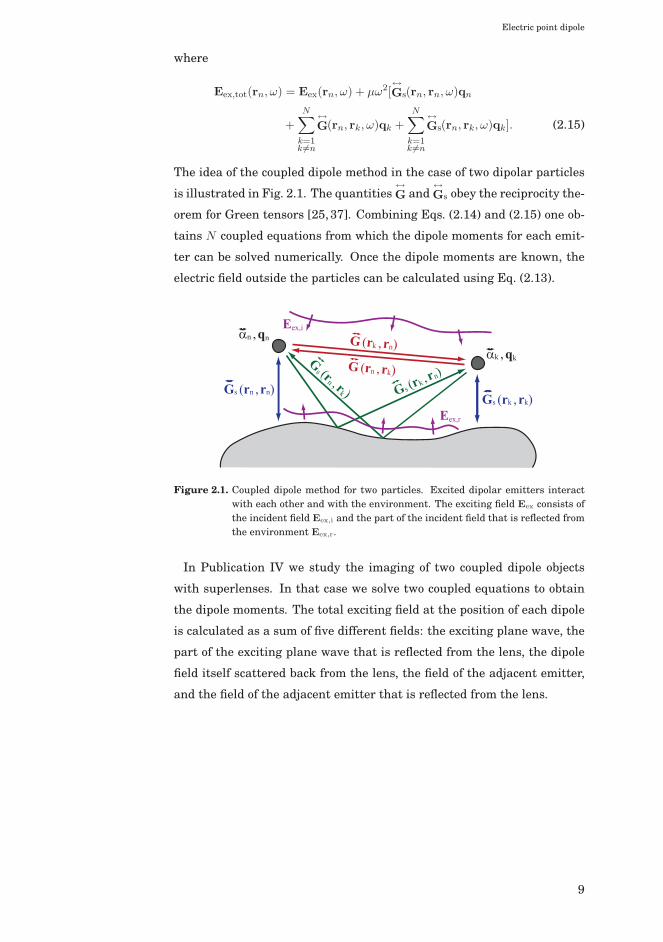
The idea of the coupled dipole method in the case of two dipolar particles

is illustrated in Fig. 2.1. The quantities↔G and

↔Gs obey the reciprocity the-

orem for Green tensors [25, 37]. Combining Eqs. (2.14) and (2.15) one ob-

tains N coupled equations from which the dipole moments for each emit-

ter can be solved numerically. Once the dipole moments are known, the

electric field outside the particles can be calculated using Eq. (2.13).

Eex,i

Gs (rk , rk)Gs (rn , rn) Gs (rk , rn)

Gs (rn , rk)

G (rk , rn)

G (rn , rk)

αn , qn

Eex,r

αk , qk

Figure 2.1. Coupled dipole method for two particles. Excited dipolar emitters interactwith each other and with the environment. The exciting field Eex consists ofthe incident field Eex,i and the part of the incident field that is reflected fromthe environment Eex,r.

In Publication IV we study the imaging of two coupled dipole objects

with superlenses. In that case we solve two coupled equations to obtain

the dipole moments. The total exciting field at the position of each dipole

is calculated as a sum of five different fields: the exciting plane wave, the

part of the exciting plane wave that is reflected from the lens, the dipole

field itself scattered back from the lens, the field of the adjacent emitter,

and the field of the adjacent emitter that is reflected from the lens.

9


10

3. Electric field of a point dipole in athree-layer structure

For many purposes in optics it is convenient to express fields by employing

the angular spectrum representation, i.e., a superposition of plane waves

(see App. A.6) [37–39]. We use this approach in Publications I–IV for the

calculation of the electric field, produced by a point source, on both sides

of the superlens structures. This method is also employed in Publication

V where we develop an arbitrary electromagnetic field as a composition of

plane waves. This chapter summarizes the steps for expressing the elec-

tric field of a point dipole in terms of the angular spectrum representation.

3.1 Angular spectrum representation of dipole field

The diverging scalar spherical wave in Eq. (2.3) can be written using the

Weyl representation [38]

eikR

R=

i2π

∫∫ ∞

−∞1kz

ei[kx(x−x0)+ky(y−y0)+kz |z−z0|]dkxdky, (3.1)

which gives the field in the half-spaces z ≤ z0 and z ≥ z0 as an angular

spectrum of plane waves. The components of the wave vector are denoted

by kx, ky, and kz in Eq. (3.1). This expression contains both the propagat-

ing waves (kz = +[k2 − (k2x + k2

y)]1/2, k2

x + k2y ≤ k2) and the evanescent

waves (kz = +i[(k2x + k2

y)− k2]1/2, k2x + k2

y > k2). In an absorbing material,

the wave vector is always complex and I speak of slowly decaying and fast

decaying waves when we refer the waves related to the low and the high

spatial frequencies, respectively (see App. A6).

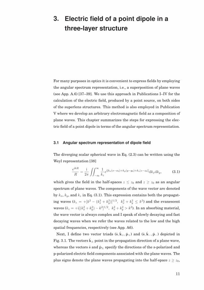
Next, I define two vector triads (s, k+, p+) and (s, k−, p−) depicted in

Fig. 3.1. The vectors k± point in the propagation direction of a plane wave,

whereas the vectors s and p± specify the directions of the s-polarized and

p-polarized electric field components associated with the plane waves. The

plus signs denote the plane waves propagating into the half-space z ≥ z0,

11

Electric field of a point dipole in a three-layer structure

and the minus signs refer to those propagating into the half-space z ≤ z0.

The vector triads satisfy the relation [40]

s× k± = p±, (3.2)

with

s = k‖ × uz, (3.3)

k‖ = k‖/√

k2x + k2

y, (3.4)

k‖ = kxux + kyuy, (3.5)

k± = k±/k, (3.6)

where k± = k‖ ± kzuz and ux, uy, uz denote the unit vectors in the Carte-

sian system. The z axis, representing the main direction of propagation,

and the vector k‖ specify the plane of incidence which determines the s

and p polarizations. I note that the vector triads defined by Eqs. (3.2)–

(3.6) are orthogonal and right-handed but k±, and thus also p±, are not

normalized in the sense of complex-valued vectors [41].

z

<

k-

z = z 0

p-

<s

<

<

k+p+

<

s

<

Figure 3.1. Illustration of the orthogonal, right-handed vector triads (s, k±, p±) in theCartesian coordinate system. The plus signs denote the plane wave prop-agating into the half-space z ≥ z0, whereas the minus signs refer to thepropagation into the half-space z ≤ z0.

After substitution of the Weyl representation into Eq. (2.2) and some

algebraic manipulation the Green tensor takes the form

↔G (r, r0, ω) =

i8π2

∫∫ ∞

−∞1kz

(ss + p±p±) ei[k‖·(r‖−r‖,0)±kz(z−z0)]dkxdky, (3.7)

where r‖ = (x, y) and r‖,0 = (x0, y0). Consequently, the dipole electric field

can be written as

E(r, ω) =iμω2

8π2

∫∫ ∞

−∞1kz

(ss + p±p±) · q ei[k‖·(r‖−r‖,0)±kz(z−z0)]dkxdky. (3.8)

With this equation the dipole field is expressed as a superposition of elec-

tromagnetic plane waves which propagate in various directions specified

12


by k± = (k‖,±kz), and whose s- and p-polarized amplitudes are propor-

tional to s ·q and p± ·q, respectively. It follows that a dipole aligned along

the z axis (q ∝ uz) creates no s-polarized components.

3.2 Reflection and transmission coefficients for a three-layerstructure

The superlens geometries analyzed in Publications I–IV are three-layer

slab structures. To calculate the dipole field transmitted through and

reflected from the lens, one needs to define the transmission and reflection

coefficients for the geometry. In this section, I introduce two different

ways for doing that.

3.2.1 Boundary condition method

One way to obtain the reflection and transmission coefficients for a three-

layer structure is to use the electromagnetic boundary conditions (see

App. A.7). In this approach, the first medium contains an incoming plane

wave and a wave reflected from the structure. Correspondingly, in the sec-

ond medium there exist two waves with one propagating in each direction,

whereas in the third medium there is only one wave moving away from

the second boundary. The detailed derivation of the transmission and re-

flection coefficients from the boundary conditions is given in Publication

III, and the idea is illustrated in Fig. 3.2.

d

E1+

I II III

E1-

E2+

E2-

E3+

Figure 3.2. Boundary condition method: the plane waves propagate in each medium andthe amplitude ratios are calculated using the boundary conditions at thefront and rear interface of medium II.

The plane waves in different layers are expressed in terms of s-polarized

and p-polarized components using the vector base defined in Sec. 3.1, and

13


referred to a common origin. Then, the boundary conditions are applied

at both interfaces which enable the calculation of the ratios between the

amplitudes of the reflected and the incident field (Rs,p = Es,p1−/Es,p

1+), as

well as between the transmitted and the incident field (Ts,p = Es,p3+/Es,p

1+).

Consequently, one obtains

Rs,p = rs,p12 + rs,p

23 ts,p12 ts,p21 e2ikz2d/(1− rs,p21 rs,p

23 e2ikz2d), (3.9)

Ts,p = ts,p12 ts,p23 eikz2de−ikz3d/(1− rs,p21 rs,p

23 e2ikz2d), (3.10)

where ts,pij and rs,pij denote, respectively, the Fresnel transmission and re-

flection coefficients for a single interface separating the media i and j,

with i, j = (1, 2, 3) (see App. A.8). In addition, kz2 = k′z2 + ik′′z2 is the z

component of the wave vector in the absorbing medium II, with k′z2 > 0,

k′′z2 > 0 for conventional (positive-index) media, and k′z2 < 0, k′′z2 > 0 in the

case of negative-index materials. The choice of the sign for the z compo-

nent of the wave vector is described in Publication I. The procedure does

not require the knowledge of the fields in medium II and is valid for both

slowly decaying (propagating) and fast decaying (evanescent) waves, as it

is a direct consequence of Maxwell’s equations.

3.2.2 Partial-wave summation method

The reflection and transmission of plane waves by a three-layer struc-

ture can also be treated by partial-wave summation. In this approach,

one considers the propagation of each plane-wave component of the dipole

field separately and employs a superposition principle. This procedure is

described in Publication I and the idea is illustrated in Fig. 3.3.

d

Einc

I II III

Er1

Er2

Et2

Et1

Figure 3.3. Principle of the partial-wave summation method: each plane wave compo-nent is multiply reflected in a three-layer structure and the partial wavesare summed up at the front and rear interface of medium II.

14


The transmission and reflection of a single plane wave at each inter-

face of the structure can be treated by using the Fresnel coefficients. One

takes also into account the multiple reflections and related propagations

inside the slab and sums all the multiply reflected waves at the front or

rear interface of medium II. The summation leads to a geometric series for

which the condition of convergence is satisfied in the case of the slowly de-

caying (propagating, low spatial-frequency) waves, in absorbing negative-

index and positive-index slab materials. The convergence condition may

fail with the fast decaying (evanescent, high spatial-frequency) waves for

both types of materials, but the summing of such divergent series is con-

ventionally justified in terms of the analytic continuation [42–44]. By

carrying out the summations, one ends up exactly with the same trans-

mission and reflection coefficients for the slab, Eqs. (3.9)–(3.10), as em-

ploying the boundary conditions. However, I want to emphasize that with

the boundary conditions no argument of analytic continuation is required.

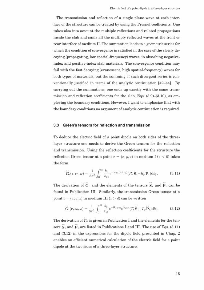
3.3 Green’s tensors for reflection and transmission

To deduce the electric field of a point dipole on both sides of the three-

layer structure one needs to derive the Green tensors for the reflection

and transmission. Using the reflection coefficients for the structure the

reflection Green tensor at a point r = (x, y, z) in medium I (z < 0) takes

the form

↔Gr(r, r0, ω) =

i8π2

∫ ∞

0

k‖kz1

e−ikz1(z+z0)(Rs

↔Sr+Rp

↔Pr)dk‖. (3.11)

The derivation of↔Gr and the elements of the tensors

↔Sr and

↔Pr can be

found in Publication III. Similarly, the transmission Green tensor at a

point r = (x, y, z) in medium III (z > d) can be written

↔Gt(r, r0, ω) =

i8π2

∫ ∞

0

k‖kz1

e−ikz1z0eikz3z(Ts

↔St+Tp

↔Pt)dk‖. (3.12)

The derivation of↔Gt is given in Publication I and the elements for the ten-

sors↔St and

↔Pt are listed in Publications I and III. The use of Eqs. (3.11)

and (3.12) in the expressions for the dipole field presented in Chap. 2

enables an efficient numerical calculation of the electric field for a point

dipole at the two sides of a three-layer structure.

15


16

4. Optical properties of superlensmaterials

The electric permittivity and the magnetic permeability are the two fun-

damental parameters characterizing the electromagnetic properties of a

medium. In Publications I–IV we use either a silver or a slightly ab-

sorbing metamaterial slab as the imaging element of the superlens struc-

tures. This Chapter deals with the optical properties of these materials:

the electromagnetic response is specified and resulting phenomena, which

are important for our studies, are described. I also give an overview on

the progress of the present metamaterial designs and discuss briefly the

applications of metamaterials.

4.1 Metals

The optical properties of metals have been discussed by many authors

[10,45]. I follow a classical picture describing the light-metal interactions.

4.1.1 Electromagnetic response of metals

The optical properties of metals are mainly due to the response of the

free conduction electrons to light. A simple way to describe the response

of the free electrons to an electromagnetic field is the Drude model [10,

45]. According to this model the relative dielectric permittivity of a metal

takes the form [10]

εr,Drude(ω) = ε′r + iε′′r = 1− ω2p

ω2 + Γ2+ i

Γω2p

ω(ω2 + Γ2), (4.1)

where ε′r and ε′′r represent the real and the imaginary part of the permittiv-

ity, respectively, and Γ is a damping constant due to scattering processes

of electrons. The quantity ωp = (Ne2/meε0)1/2 is known as the volume

plasma frequency, with e being the electron charge, N the number of elec-

trons per unit volume, and me the effective mass of electrons. Metals do

17

Optical properties of superlens materials

not have magnetic response at the optical frequencies, i.e., μr = 1.

From Eq. (4.1) it is seen that ε′r is negative when ω2 < ω2p, but still

ω2 � Γ2, which is usually the case at optical frequencies [45]. For in-

stance, gold has ωp = 13.8 · 1015 s−1 and Γ = 1.075 · 1014 s−1 making the

real part of the permittivity negative over the visible range [10]. The neg-

ative value of ε′r reflects the fact that the electrons oscillate out of phase by

π radians with the exciting field [10,45]. The negative real part of permit-

tivity leads to a large imaginary part of refractive index (n =√

εr), which

makes the metal highly reflective [45]. The imaginary part of the refrac-

tive index, and consequently the reflectivity, becomes high also when ε′′ris large which is the case for sufficiently low values of ω (in the infrared

regime). On the other hand, when ω2 > ω2p (but ω2 � Γ2) the real part

of the permittivity is positive and ε′′r is small compared to ε′r. Thus, the

metal behaves essentially as a dielectric material. The Drude model is

sufficiently accurate at the infrared frequencies and consequently widely

used in optics. However, it needs to be supplemented in the visible regime

by the influence of the bound electrons which results in the dielectric con-

stant to exhibit a resonant behavior [10].

Most metals, and especially noble metals, indeed possess a negative real

part of the permittivity at the optical frequencies. Widely used values

for noble metals are the ones retrieved experimentally by Johnson and

Christy [46]. One may note that these are the bulk values which are

valid as long as the dimensions of the metal structures are larger than

the electron mean free path (∼ 10 nm in silver) [10]. When considering

nanometer-scale metal films or very small metal nanoparticles the size

corrections to the bulk values need to be taken into account [47]. In Pub-

lications II–IV we study the near-field imaging with silver superlenses

having the silver layer thickness varying from 15 nm to 50 nm, and in

line with few recent superlens experiments [14,15], we use the bulk value

(εr = −2.4 + i0.2 at λ = 365 nm [46]) for the silver permittivity.

4.1.2 Surface plasmons

Among the most fascinating consequences of the interaction of metal nanos-

tructures with light is the possibility to excite plasmons [10,48,49]. Plas-

mons localized in more dimensions than one can be excited in metallic

particles, nanowires, or other nanostructures [48–52]. These local surface

plasmons are different from surface plasmon polaritons [53, 54]. Surface

plasmon polaritons are surface-charge-density oscillations that may exist

18


at the interface of two media having dielectric constants of opposite signs.

Research in the field of optics making use of plasmons is mostly concerned

with the control of optical radiation on the subwavelength scale [55–58].

This field has progressed rapidly during the recent years and developed

into a research area of its own known as plasmonics [59,60].

I first consider a single planar interface between two materials. The

first medium is characterized by its complex, frequency-dependent dielec-

tric permittivity εr1 = ε′r1+iε′′r1, while the second one is a dielectric material

having real permittivity εr2. Using a plane wave approach and applying

the electromagnetic boundary conditions at the interface one can find so-

lutions of the Maxwell equations which are localized at the boundary:

field modes that propagate along the interface and decay exponentially

orthogonal to it. Surface plasmon polaritons of this kind are generated by

the surface plasmons and in non-magnetic materials (μr1 = μr2 = 1) these

fields are purely p-polarized. The existence conditions and the character-

istic properties, such as the propagation distance and the decay length on

both sides of the interface, of surface plasmon fields are derived in many

textbooks [10, 48, 49]. Surface plasmon polaritons can exist if the real

parts of the permittivities of the two media possess opposite signs. Met-

als, especially noble metals, have negative real part and sufficiently small

imaginary part at optical frequencies, and thus interfaces between met-

als and dielectrics can support polaritons. Surface plasmon polaritons

can only be excited by an external field whose wave vector component

along the interface is larger than the free-space wave number. Therefore

polaritons are normally created by employing gratings or total internal

reflection (evanescent wave) in prisms [52].

Surface plasmons can also be excited on the boundaries of a metal film

embedded between dielectric media. Well-known experimental arrange-

ments are the Otto and Kretschmann configurations in which an evanes-

cent wave generated by total internal reflection excites polaritons on the

surface of a thin metal layer. The existence of the surface plasmons in

these setups is manifested by the minimum of the reflected illumination

as the energy is transferred to the polariton. At the same time, the inten-

sity of the electric field on the metal surface representing the polariton is

strongly enhanced [10, 49]. This corresponds to a near-singularity of the

transmission (and reflection) coefficient from the evanescent wave in the

metal film to the polariton field. In the three-layer structures of metallic

superlenses similar phenomena take place. High spatial-frequency com-

19


ponents of the field generated by the object are coupled into the metal

layer and enhanced by surface plasmons on both interfaces.

In Publications II–IV we consider a thin silver layer as the near-field

imaging element. The operation of the silver lens is based on the electric

field enhancement of the p-polarized evanescent wave components of the

dipole radiation on the metal boundaries due to the excitation of surface

plasmons.

4.2 Metamaterials

During the last ten years there has been a strong interest in novel optical

media called metamaterials [2–6]. Metamaterials are artificially engi-

neered structures possessing extraordinary physical properties, unavail-

able in naturally occurring materials, when interacting with an electro-

magnetic field. The rapid progress in this field has offered an entirely new

route to design material properties at will.

4.2.1 Material parameters of metamaterials

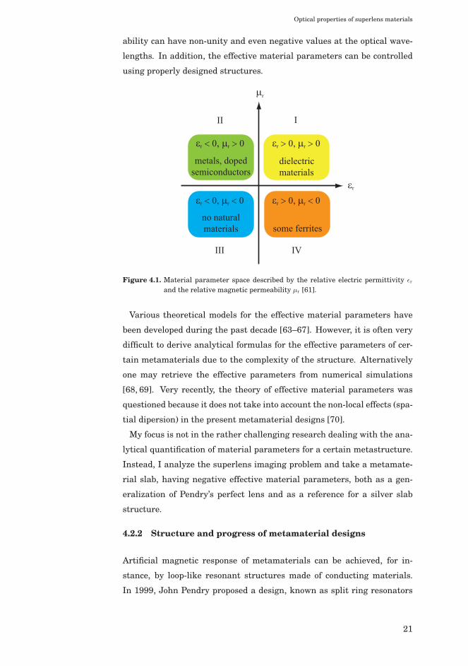
An illustrative way to represent the electromagnetic properties of all ma-

terials is to use ‘a material parameter space’ shown in Fig. 4.1 [61]. In

this picture, quadrant I contains materials with positive permittivity and

permeability, i.e., most dielectric materials. Region II covers metals, fer-

roelectric materials, and doped semiconductors which can have negative

permittivity at certain frequencies. Quadrant IV is composed of few fer-

rite materials having negative permeability at some frequencies [61]. How-

ever, this kind of magnetic response fades away above the microwave fre-

quencies and in the optical regime μr = 1 holds for all naturally existing

materials [62]. Region III embraces metamaterials for which the perme-

ability and the permittivity are simultaneously negative, but in nature,

materials of this type do not exist. Metamaterials consist of periodically

or randomly structured sub-units whose size and separation are much

smaller than the wavelength of an electromagnetic field. Consequently,

microscopic details of individual structure elements can not be sensed by

the field, but the average of the assembly’s collective response matters.

The electromagnetic response of this kind of material can be character-

ized by an effective relative permittivity εr,eff and permeability μr,eff . What

makes the metamaterials attractive is the fact that the effective perme-

20


ability can have non-unity and even negative values at the optical wave-

lengths. In addition, the effective material parameters can be controlled

using properly designed structures.

III

III IV

μr

εr

εr > 0, μr > 0εr < 0, μr > 0

εr > 0, μr < 0εr < 0, μr < 0

dielectric materials

metals, doped semiconductors

no natural materials some ferrites

Figure 4.1. Material parameter space described by the relative electric permittivity εr

and the relative magnetic permeability μr [61].

Various theoretical models for the effective material parameters have

been developed during the past decade [63–67]. However, it is often very

difficult to derive analytical formulas for the effective parameters of cer-

tain metamaterials due to the complexity of the structure. Alternatively

one may retrieve the effective parameters from numerical simulations

[68, 69]. Very recently, the theory of effective material parameters was

questioned because it does not take into account the non-local effects (spa-

tial dipersion) in the present metamaterial designs [70].

My focus is not in the rather challenging research dealing with the ana-

lytical quantification of material parameters for a certain metastructure.

Instead, I analyze the superlens imaging problem and take a metamate-

rial slab, having negative effective material parameters, both as a gen-

eralization of Pendry’s perfect lens and as a reference for a silver slab

structure.

4.2.2 Structure and progress of metamaterial designs

Artificial magnetic response of metamaterials can be achieved, for in-

stance, by loop-like resonant structures made of conducting materials.

In 1999, John Pendry proposed a design, known as split ring resonators

21


(SRR), for obtaining negative magnetic permeability [63]. The route to

manufacture metamaterials with a negative effective refractive index is

to combine two sets of structures with Re(εr,eff) < 0 and Re(μr,eff) < 0 in

the same frequency range. This kind of structure, operating at the mi-

crowave frequencies and consisting of copper SRRs and wires, was first

experimentally demonstrated in 2000 [64]. After that several SRR-based

metamaterial designs have been advanced from microwave frequencies to

the optical regime by scaling down the structure size [71–76]. However, it

was found that the magnetic response of SRRs decreases with the down-

scaling of the structure, and negative values of the permeability can not

be reached at the visible region [77,78].

Another proposed metamaterial design is a nanorod structure for which

negative refractive index is reported at telecommunication wavelengths

and even in the red part of the visible spectrum [79–82]. The most suc-

cessful optical NIM structure so far is the fishnet structure which has

recently brought the negative refractive index from the infrared regime

to the visible wavelengths and enabled the fabrication of bulk metamate-

rials [83–88]. One of the major challenges of optical NIMs based on res-

onant structures is the strong energy dissipation of the electromagnetic

field. A possible way of addressing this issue is to incorporate gain media

into NIM designs [89, 90]. An alternative route towards the NIMs is the

to use chiral materials [91–94]. Negative refraction is also demonstrated

in semiconductor metamaterials [95].

The amount of losses in NIMs is often described by the figure of merit

(FOM = −Re(n)/Im(n)). The most promising optical NIM designs pro-

posed so far are a low-loss bulk NIM (FOM 3.5) working at near-visible

wavelengths [86], a loss-free and active NIM operating in the red part of

the visible spectrum [90], and a bistable and self-tunable NIM structure

(FOM 8.5) working at λ = 650 nm [96].

4.2.3 Electromagnetic properties of NIMs

The idea of NIMs was actually born in the early 20th century among the

works on a negative phase velocity and its consequences [4]. Later, in the

forties and fifties the optical properties of NIMs were studied by Russian

physicists [4]. The most well known step was made by Veselago in 1967

with a systematic study on the electromagnetic properties of materials

having negative material parameters [1]. However, at that time no ma-

terials were available for testing Veselago’s ideas and they remained as a

22


scientific curiosity until Pendry inspired the recent boom on NIMs [63].

Veselago considered monochromatic plane waves in a lossless medium

having real and negative permittivity and permeability. Starting from

the Maxwell equations he showed that the wave vector k, the electric field

E, and the magnetic field H of a plane wave form a left-handed triad in

medium with εr < 0, μr < 0, whereas in a normal medium the triplet

is right-handed. Due to this property materials with simultaneoustly

negative permittivity and permeability are called left-handed materials

(LHMs). Moreover, the Poynting vector defined as S = E ×H is antipar-

allel to the wave vector k in LHMs. It was also proven that the refractive

index given by n = ±√εrμr must take the negative value which is the

reason for the often used term negative-index materials. Veselago fur-

ther pointed out that if light is incident from a positive-index material

to a NIM, the refracted light lies on the same side as the incident one

with respect to the surface normal - the effect known as negative refrac-

tion. These phenomena are illustrated in Fig. 4.2. In addition, Veselago

showed that the Doppler effect and the Cherenkov effect are reversed in

NIMs [1].

In Publications I, III, and IV we consider slightly absorbing metamate-

rial, having εr = ε′r + iε′′r and μr = μ′r + iμ′′r , with ε′r, μ′r < 0 and ε′′r , μ′′r being

small positive numbers, as a superlens material. For our studies, an im-

ki

Ei

Hi

kt

Et

Ht

εi > 0μi > 0ni > 0

εt < 0μt < 0nt < 0St

Si

Figure 4.2. Illustration of the counterintuitive electromagnetic properties of negative-index materials proposed by Veselago [1]. The subscript i denote the mediumof incidence (conventional, positive-index material) and t the medium oftransmittance (NIM). The wave vector k, the electric field E, and the mag-netic field H of a plane wave constitute a left-handed triad in NIMs, whereasin conventional materials the triplet is right-handed. Negative refractiontakes place at the interface of positive and negative-index materials. Thewave vector k and the Poynting vector S are antiparallel in NIMs, while inpositive-index materials they are parallel.

23


portant consequence of the negative ε′r and μ′r is the fact that the sign of

the real part of wave vector’s z-component (the component along the prop-

agation direction) is reversed: kz,2 = k′z,2 + ik′′z,2, with k′z,2 < 0, k′′z,2 > 0.

This result is derived in Publication I using the theory of complex func-

tions, in a manner following an earlier study [97]. Another remarkable

point to notice is the magnetic response (μr �= 1) of our NIM lens material.

As mentioned in Sec. 4.1.2 the fields generated by the surface plasmons

are purely p-polarized which results from the absence of the magnetic re-

sponse of metals at the optical range. If the material has a negative real

part of the permeability, plasmon-like magnetic resonances can occur for

s-polarized light as well [52]. This effect leads to a greater enhancement

of the evanescent wave components of the object radiation in transmission

through a metamaterial slab than through a silver slab in which only the

p-polarized waves are amplified.

4.2.4 Applications of metamaterials

Due to their unusual properties metamaterials have a number of poten-

tial uses. At microwave frequencies metamaterials have already been em-

ployed in various applications, such as magnetic resonance imaging [98],

compact waveguides [99], novel microwave circuits [100], and microwave

antennas [101]. One attractive metamaterial device is the perfect lens

providing an image resolution beyond the diffraction limit [13]. The con-

cept of perfect lens (superlens) has been demonstrated experimentally at

microwave, mid-infrared, and optical frequencies [7]. Another hot topic

within the metamaterial community is the control of the flow of light in

desirable manners which enables, for instance, to design cloaking devices

making objects invisible or less detectable [8, 9]. Further, tunable meta-

materials can be used for modulating and switching EM waves at tera-

hertz frequencies [102]. An interesting application of metamaterials are

also perfect absorbers making the individual absorption of the electric and

magnetic components of EM waves possible [103].

As mentioned before, this thesis concerns two applications of metama-

terials: Publications I–IV focus on the superlenses, whereas Publication

V deals with optical cloaking. The principles and our main results related

to these topics are introduced in the following two chapters.

24

5. Near-field imaging with slabsuperlenses

Most of this thesis is focused on near-field imaging of dipole-like objects

with silver and slightly absorbing NIM superlenses. In this chapter, I first

introduce the concepts for defining the resolution of an imaging system.

Then, I show how the perfect lens and its physical realizations, known as

superlenses, work as an imaging device. I also give an overview on the re-

cent development on near-field superlenses. The last section summarizes

the research reported in Publications I–IV.

5.1 Resolution in far-field imaging

Spatial resolution is a measure of the capability to distinguish two sep-

arated objects. The diffraction limit states that the resolution in optical

imaging is limited by the wavelength of light and the numerical aperture

(NA) of the instrument. However, the near-field imaging techniques al-

low us to access the evanescent wave components of the object radiation

which effectively increase the NA and leads to spatial resolutions beyond

the diffraction limit [10,12].

5.1.1 Point-spread function

The point-spread function (PSF) defines the resolution of an optical imag-

ing system. The image of a radiating point source appears to have a finite

size, and as the name indicates, PSF describes the spread of the field

created by a point source in an imaging process. This broadening is a con-

sequence of spatial filtering: a point source in space is characterized by a

delta function and its radiation embraces the infinite spectrum of spatial

frequencies, but on propagation from the object to the image, high-spatial-

frequency components (evanescent waves) are filtered out. In addition, all

propagating waves cannot either be collected due to the finite size of the

25

Near-field imaging with slab superlenses

lenses which leads to a further reduction in bandwidth. With the reduced

spectrum of the object radiation a part of information is lost in the imag-

ing process and a complete reconstruction of the original point source in

the image is not possible.

The classic theory of diffraction of electromagnetic fields by optical sys-

tems is that of Richards and Wolf [104]. The smallest radiating elec-

tromagnetic unit is a point dipole, and as discussed in Chap. 2, most

subwavelength-sized particles scatter as electric dipoles in the optical

regime. The imaging of a dipole by aplanatic lens systems (obeying the

sine condition [105]), in which the distance between the object and the

image is much larger than the wavelength of light, has been analyzed

by many authors [10, 106, 107]. The quantity |E|2, where E is the dipole

field in the image region, is often used to denote the point-spread func-

tion since it is relevant to optical detectors. If the optical axis of such

systems is along the z direction, the transverse PSF is calculated in the

image plane as |E(x, y, z = constant)|2 (see Fig. 5.1). For dipoles aligned

perpendicular to the axis the distribution of |E|2 in paraxial approxima-

tion is slightly broader in the direction of the dipole than orthogonal to

it, in excellent agreement with the exact calculation [10]. The character-

istic widths of these profiles specify the size Δr of the PSF. In contrast,

the field strength along the optical axis in the image area, calculated as

|E(x = 0, y = 0, z)|2, gives the axial PSF (see Fig. 5.1). Its characteristic

width Δz gives the depth of field. The quantities Δr and Δz depend on

both the magnification (M ) and the numerical aperture (NA) of the imag-

ing system. As an example, for a typical microscope objective with M = 60

and NA = 1.4, and for wavelength λ = 500 nm, one obtains Δr ≈ 13 μm

and Δz ≈ 1.8 mm [10].

Δr optical system

Δz

image plane

Figure 5.1. Illustration of the transverse (blue curve) and axial (orange curve) point-spread functions (PSFs) characterized by the widths Δr and Δz, respectively.In electromagnetic imaging the transverse width depends on the direction inthe image plane and the orientation of the object dipole.

26


In electromagnetic imaging the PSF depends strongly on the orienta-

tion of the dipole. In conventional far-field systems the image has a clear

peak-shaped profile if the dipole is oriented perpendicular to the optical

axis. On the other hand, for a dipole aligned along the axis, the image-

intensity distribution is zero on the optical axis and contains two peaks

on both sides of the axis. In the latter case it is more difficult to define the

characteristic width of the transverse PSF. The image of a dipole along

optical axis is a bit wider than the image of a dipole oriented perpendic-

ular to the axis [10]. The situation is different in near-field imaging with

slab lenses, as will be seen in Sec. 5.4.

5.1.2 Diffraction limit

Now, as we have seen how a single point-like object is mapped to the im-

age, our next task is to define how two point dipoles that are separated

by a distance Δr‖ = [(Δx)2 + (Δy)2]1/2 can be distinguished. When mov-

ing two point emitters in the object plane closer to each other, their PSFs

in the image start to overlap. At some point, two emitters become indis-

tinguishable. If the point sources are uncorrelated one can view them as

resolvable if the maxima of their PSFs in the image are separated by more

than the characteristic width of one individual PSF. Accordingly, a narrow

PSF leads to a better resolution than a wider one.

As mentioned in the last section, the resolving capability of an imaging

system depends on the bandwidth of spatial frequencies that are collected

by the system:

Δk‖ = [(Δkx)2 + (Δky)2]1/2. (5.1)

Straightforward Fourier analysis leads to a relation [37,108]

Δk‖Δr‖ ≥ 1, (5.2)

where Δk‖ and Δr‖ are the rms widths and Δr‖ gives the minimum resolv-

able separation in the object plane. In far-field imaging only propagating

waves are collected: the upper bound for Δk‖ is defined by the wave num-

ber k = 2πn/λ, with n being the refractive index of the medium in which

the object is located. Thus, the minimum for the spatial resolution is

Min[Δr‖] =λ

2πn. (5.3)

However, the entire spectrum of propagating waves cannot be collected

and the resolution limit is affected by the NA of the imaging system.

27


The theoretical limit for the resolution of a microscope is often taken

to follow Abbe’s or Rayleigh’s early works [45]. Both Abbe and Rayleigh

state that two point-like objects are distinguished if the maximum of one

paraxial PSF in the image coincides with the first minimum of the second

PSF. In that case, the ratio of the intensity minimum at the midpoint of

the image distribution to the intensity maximum is 0.81. This kind of

analysis leads to [10,45]

Min[Δr‖]Abbe−Rayleigh = 0.61λ

NA≈ λ

2NA. (5.4)

Abbe’s formulation is based on the paraxial approximation and only the

special case of two parallel dipoles aligned perpendicular to the optical

axis is analyzed [10]. If the dipoles are aligned parallel to the optical axis

the definition of the resolution limit becomes somewhat arbitrary due to

the shape of the PSFs, as discussed in the previous section.

According to Eq. (5.2) the resolution is unlimited if the bandwidth of the

object radiation in the image is arbitrarily large. Going beyond the limit

given in Eq. (5.3) requires the detection of the evanescent wave compo-

nents which is the subject of near-field imaging techniques [10, 12]. Pub-

lications I–IV deal with the near-field imaging with the superlenses and

the remaining part of this chapter concerns that topic.

5.2 The perfect lens

The idea of the perfect lens was born in Veselago’s early studies in 1967

dealing with the electromagnetic properties of NIMs [1]. However, the

increased number of works concerning this unconventional lens were not

inspired until John Pendry complemented Veselago’s ideas in 2000 [13].

5.2.1 Focusing of propagating waves

The perfect lens is a transversally infinite, flat slab of ideal NIM that is

surrounded by vacuum. The refractive index of the perfect lens material

equals −1 and the lens thickness is d. If an object is located at a distance

a (a < d) in front of the slab, the image at the distance d − a behind the

slab will be perfect. Veselago introduced the idea of the perfect lens us-

ing ray optics [1]. He proposed that light rays emerging from the object

exhibit negative refraction at the interfaces of the NIM slab. Negative

refraction allows the flat slab to focus all the diverging light rays from the

point object into a point behind the slab. Other characteristics of the sys-

28


tem include a double focusing effect – another image is formed inside the

slab. The focusing action of the perfect lens is illustrated in Fig. 5.2(a).

The relative permittivity and permeability of NIM slab are equal in mag-

nitude but opposite in sign to those of vacuum, i.e., εr2 = −1, μr2 = −1,

making the Fresnel reflection coefficients zero. Consequently, the inter-

faces of the lens show no reflection and the light is perfectly transmitted

through it. However, one may note that the perfect lens is not a lens in

the conventional sense of the word since it can not focus normally incident

light.

da d - a

εr1 = 1μr1 = 1n1 = 1

(a) (b)

object plane object planeimage plane image plane

evanescent waves

propagating waves

da d - a

εr1 = 1μr1 = 1n1 = 1

εr2 = -1μr2 = -1n2 = -1

εr1 = 1μr1 = 1n1 = 1

εr1 = 1μr1 = 1n1 = 1

εr2 = -1μr2 = -1n2 = -1

Figure 5.2. Transversally infinite flat slab acts as the perfect lens. The thickness of theslab is d, the refractive index equals −1, and the slab is surrounded by vac-uum. The slab (a) brings all propagating light rays from the object plane intoa focused image, and (b) enhances the evanescent waves so that the net am-plitude change between the object and image plane is zero (red dashed line,see Eq. (5.12)). The increase of the amplitudes takes place at the boundariesdue to surface resonances, as discussed in the main text.

In his famous paper, Pendry applied a plane-wave approach to analyze

the imaging with the perfect lens [13]. When considering the propagating

waves of the object radiation Pendry stated that the transport of energy

in the propagation direction of the plane wave (+z direction) implies the

conventional choice of the positive sign for the wave vector’s z component

in vacuum, but in NIM the negative sign for the z component is required:

kz1 = +√

εr1μr1k20 − (k2

x + k2y), k2

x + k2y ≤ εr1μr1k

20, (5.5)

kz2 = −√

εr2μr2k20 − (k2

x + k2y), k2

x + k2y ≤ εr2μr2k

20. (5.6)

Here k0 is the wave number in vacuum, subscript 1 denotes the vac-

uum (medium I) surrounding the lens and 2 refers to the lens material

(medium II). Together with the material parameters εr1 = μr1 = 1 and

εr2 = μr2 = −1, Eqs. (5.5) – (5.6) lead to the Fresnel reflection and trans-

29


mission coefficients that are equal to zero and 1, respectively. Further, the

reflection and transmission coefficients of the perfect lens become [13]

Rs,p = 0, (5.7)

Ts,p = eikz2d = e−ikz1d, (5.8)

where s and p refer to the s- and p-polarized waves, respectively. From

these equations one sees that the lens reflects no light and cancels the

phase change of the propagating waves when they travel from the object

plane to the front surface of the lens, and again, from the back surface of

the lens to the image plane. Thus, Pendry’s conclusions concerning the

propagating waves match with Veselago’s ideas.

5.2.2 Enhancement of evanescent waves

The new message of Pendry’s study were his results concerning the evanes-

cent wave components of the object radiation. In contrast to the case of

the propagating waves, Pendry chose the same sign for the z components

of the wave vector in both media [13]:

kz1 = +i√

k2x + k2

y − εr1μr1k20, k2

x + k2y > εr1μr1k

20, (5.9)

kz2 = +i√

k2x + k2

y − εr2μr2k20, k2

x + k2y > εr2μr2k

20. (5.10)

These choices were justified by the fact that the evanescent waves must

decay exponentially in both media with increasing z. However, Eqs. (5.9)–

(5.10) with the material parameters εr1 = μr1 = 1, εr2 = μr2 = −1 lead to

a diverging Fresnel reflection and transmission coefficients. To avoid this

divergence, Pendry derived the reflection and transmission coefficients of

the perfect lens using the summation method, introduced in Sec. 3.2.2, in

the limit εr2, μr2 → −1. With this approach one obtains [13]

limεr2,μr2→−1

Rs,p = 0, (5.11)

limεr2,μr2→−1

Ts,p = e−ikz2d = e−ikz1d. (5.12)

Substitution of Eq. (5.9) into Eq. (5.12) implies that the amplitudes of the

evanescent waves increase in the transmission through the slab by the

same amount as they decay in free space on both sides of the slab: the

net amplitude change between the object plane and the image plane is

zero. I emphasize that the evanescent waves are not amplified on prop-

agation within the slab, but the amplitudes change at the boundaries.

This extraordinary behavior relies on the fact that NIM supports resonant

30


surface waves, one example of which are waves due to surface plasmons.

The enhancement of evanescent waves in the perfect lens is illustrated in

Fig. 5.2(b). Because evanescent waves do not carry any net energy flux,

the energy of the field is not increased and only the distribution of the

energy across the space, i.e., the energy density, is changed.

In summary, the perfect lens not only cancels the phase change for the

propagating waves, but also restores the amplitudes of the evanescent

waves which allows the creation of the perfect image with unlimited res-

olution. However, shortly after its publication Pendry’s work aroused a

fair amount of debate among the scientists [42,43,109–114]. Without tak-

ing side in the arguments I merely consider Pendry’s theory as a starting

point for a more detailed study of superlenses.

5.3 Imaging with superlenses

Negative-index materials are necessarily dispersive and hence lossy [61].

Accordingly, the material parameters of NIMs must contain the imagi-

nary parts as well, and especially, resonance-based NIMs are inherently

associated with considerable energy dissipation. Lenses that take this

practical limitation into account are known as superlenses. Despite the

rapid progress of NIMs, the realizations of NIM superlenses are few be-

cause properly working bulk NIMs are still more or less unattainable with

modern fabrication techniques. However, the subwavelength resolution

can also be achieved with physically realizable metallic slab lenses [7,13].

5.3.1 Enhancement of evanescent waves

The idea of the metallic superlens was also mentioned in Pendry’s pa-

per [13]. One can consider a slab-lens imaging system in the electro-

static (quasi-static) limit when all the dimensions of the system are much

smaller than the wavelength of light [13]:√k2

x + k2y � ω/c0 = k0, (5.13)

where c0 is the vacuum speed of light. Now, several formulas concerning

the perfect lens can be approximated by taking the limit k2x+k2

y →∞. The

z components of the wave vectors take the forms [13]

kz1 = +i√

k2x + k2

y − εr1μr1k20 ≈ +i

√k2

x + k2y, when k2

x + k2y � k2

0, (5.14)

kz2 = +i√

k2x + k2

y − εr2μr2k20 ≈ +i

√k2

x + k2y, when k2

x + k2y � k2

0, (5.15)

31


i.e., kz2 = kz1 in this limit. Using these expressions one finds that the

transmission coefficient of the slab for p polarization becomes indepen-

dent of μr, and if εr1 = 1, εr2 → −1, one obtains [13]

limεr2→−1

Tp = e+i√

k2x+k2

yd, when k2x + k2

y � k20. (5.16)

Thus, the p-polarized evanescent wave components of the object radiation

can be amplified with a slab lens having negative εr2 only. Similarly, in

the quasi-static limit Ts becomes independent of εr2 and a slab with neg-

ative permeability (μr2 = −μr1) would amplify the s-polarized evanescent

waves. The superlens effect therefore remains valid for one polarization

in a medium having only one of the material parameters negative. Natu-

ral candidates for superlens material in the case of p-polarized light are

noble metals, and especially silver, because of its low losses at optical fre-

quencies.

Shortly after the proposal of the superlens, various theoretical studies

on superlens properties were published [115–119]. These studies pre-

dicted that the subwavelength resolution is achievable with silver super-

lenses, but only with a carefully chosen design. At first, the distance be-

tween the slab and the object and image planes, as well as the slab’s thick-

ness must be small compared with the wavelength. In addition, the losses

of the lens material need to be small, and a good impedance match (i.e.,

negligible reflections at the interfaces) between the lens and its environ-

ment is required. It appears that the quantities which describe the imag-

ing capability of superlenses are the slab’s transmission coefficients. The

losses, even very small ones, change the behavior of the slab’s transmis-

sion coefficients from exponentially growing (see Eqs. (5.12) and (5.16))

to peak-shaped exceeding unity only at a certain range of high spatial

frequencies. Consequently, the feature that crucially separates the super-

lenses from the conventional ones is that the resolution is not limited by

diffraction, but rather defined by how much and in how wide a range of

spatial frequencies the evanescent waves are enhanced.

5.3.2 Development of near-field superlenses

Pendry’s proposal inspired also experimental attempts to test the super-

lens concept in practice. First, the enhancement of the evanescent waves

across the slab was demonstrated [120, 121]. These studies brought out

valuable suggestions concerning the slab thickness and surface roughness

requirements. During the years 2003 and 2004 the first superlens designs

32


providing a subwavelength resolution at microwave frequencies were re-

alized [122–124]. In 2005, the superlensing effect was observed in the

optical range [14,15].

Figure 5.3 shows the cross-section of the superlens structure reported in

Refs. [14,15]. In that design a thin silver film with the optimized thickness

of 35 nm is embedded between two dielectric materials. The first dielectric

medium in front of the silver slab is a polymethyl methacrylate (PMMA)

spacer layer having the thickness of 40 nm. The second one behind the

silver layer is a photoresist (PR) used for recording the image. The object

is a 2D chromium grating or an arbitrary 2D object patterned on top of the

PMMA spacer. The object is illuminated from behind with a light having

λ0 = 365 nm (I-line of the mercury lamp). At this wavelength silver shows

a negative real part of the permittivity and the impedance match with

the dielectrics is good: εPMMA ≈ 2.3, εAg ≈ −2.4 + i0.2, and εPR ≈ 2.9

(while μPMMA = μAg = μPR = 1). As a consequence of the enhance-

ment of the evanescent wave components scattered from the object, the

subwavelength resolutions of λ0/6 [14] and λ0/7 [15] were demonstrated.

One of the major challenges, limiting the enhancement of the evanescent

waves and consequently the attainable resolution with silver superlenses,

is the difficulty in manufacturing smooth and flat surfaces. In 2010, an

ultra thin and smooth silver superlens was fabricated by employing a new

method utilizing Ge-Ag surface interactions [16]. With this design a 2D

grating object was imaged with a resolution of λ0/12. I also mention that

already in 2006, a low-loss SiC superlens based on surface phonons and

operating at mid-infrared frequencies (∼ 10 μm) was reported to provide

a resolution of λ0/20 [125].

PMMA

Ag

PHOTORESIST

Cr

QUARTZ

40 nm

35 nm

120 nm

50 nm120 nm

λ0 = 365 nm

Figure 5.3. Cross-section of a silver superlens structure. The image of 50 nm Cr gratingwith 120 nm period is resolved in the photoresist providing the resolution ofλ0/7 [15].

33


The superlenses discussed so far enable the construction of the image

only in the near field because the evanescent waves decay rapidly after

the lens. One of the future challenges is to bring the subwavelength im-

age into the far field. This may be possible with the so called far-field

superlenses (FSLs) which converts the evanescent waves behind the lens

into propagating ones [126], or with cylindrical hyperlenses [127]. There

already exist a few demonstrations of such lenses [128, 129]. Although

these concepts are very interesting and promising they do not fall within

the scope of this thesis.

5.4 Near-field imaging of point-like objects with superlenses

In this section I summarize our research dealing with the near-field imag-

ing of dipolar emitters with NIM and silver superlenses.

5.4.1 Imaging of a radiating dipole with NIM superlens

Publication I is a detailed study concerning electromagnetic imaging with

a slightly lossy metamaterial superlens surrounded by vacuum (see Fig. 1

in I). The object is a single radiating point dipole. The material param-

eters of the lens are close to those of the perfect lens: εr2 = −1 + iε′′ and

μr2 = −1 + iμ′′, with ε′′ and μ′′ being small positive numbers. The slab

thickness d is few tens of nanometers. The distance between the object

plane and the front surface of the slab, as well as between the rear sur-

face of the slab and the image plane are equal to d/2, in line with the

superlens system.

We first show how the sign of the wave vector in a lossy NIM can be

determined. Then, using the angular spectrum representation and the

partial-wave summation, we derive the Green tensor for the dipole field

transmitted through the slab lens. The Green tensor includes the trans-

mission coefficients of the slab, which describe the quality of the slab as

a near-field imaging device. We show how the transmission coefficients

behave as a function of spatial frequencies: the absolute values of the co-

efficients exhibit a peak-shaped behavior and exceed unity at a certain

range of the spatial frequencies (see Fig. 4 in I). This enables the en-

hancement of evanescent wave components of the object radiation, but

not over the whole range of spatial frequencies as the perfect lens would

do. Consequently, the image of a point source is a spot with a finite size.

34


When the losses or the slab thickness increase the enhancement range of

the evanescent waves moves towards lower spatial frequencies and gets

narrower because the absorption in the slab increases.

With the derived formalism we evaluate numerically the point-spread

function in the image plane behind the slab, and verify that the NIM slab

increases the resolution several orders of magnitude when compared with

conventional imaging (see Figs. 5 and 6 in I). The resolution is well beyond

the diffraction limit for both the dipole oriented parallel to the slab and

orthogonal to the slab. With numerical simulations we also point out that

the resolution of the imaging system decreases linearly as a function of d,

whereas it depends logarithmically on ε′′ and μ′′ (see Fig. 8 in I).

5.4.2 Imaging of a radiating dipole with silver superlens

In Publication II we extend our formalism, developed in Publication I, to

the case of a silver superlens. In this geometry a thin silver film is sand-

wiched between two dielectrics (see Fig. 1 in II). The first half-space before

the silver layer is composed of polymethyl methacrylate (PMMA) and the

half-space behind the lens is filled with photoresist (PR). The object plane

is located 40 nm in front of the lens and the image is considered immedi-

ately (2 nm) behind the lens. Thus, the imaging system is similar to that

used in the experiments [14,15], but our object is a radiating point dipole

instead of a two-dimensional grating or structure. The dipole, which is a

genuine three-dimensional object since the moment can be arbitrarily ori-

ented, radiates at the wavelength of λ0 = 365 nm for which εPMMA ≈ 2.3,

εAg ≈ −2.4 + i0.2, and εPR ≈ 2.9.

We show that the enhancement of the evanescent waves occurs for p po-

larization, but not for the s-polarized waves due to the lack of magnetic

response (see Fig. 2 in II). The enhancement is not as strong as with the

slightly lossy NIM because of higher losses and worse impedance match,

and again, the enhancement decreases when the slab thickness is in-

creased. Also in this study, we evaluated the PSFs in the image plane and

defined the resolution of the system (see Fig. 3 in II). Now the resolution

depends strongly on the orientation of the object dipole. The resolution

for the dipole oriented orthogonal to slab is better because the dipole field

in that case contains only p-polarized components. In contrast, the field

of the dipole aligned parallel to slab contains both polarizations, and the

s-polarized near-field components are not enhanced in transmission. We

obtained the resolutions λ0/4 and λ0/8 for the dipoles aligned parallel and

35


orthogonal to the slab, respectively. In this paper we also show that the

quasi-static approximation leads to considerable differences in the behav-

ior of the transmission coefficients for p-polarization, but accurate results

on resolution, when compared to the exact calculation.

Figure 5.4 illustrates the superlens effect of the silver slab. In Fig. 5.4(a),

the normalized intensity distribution is calculated at the plane z = 77 nm

in PMMA when the dipole is oriented along the z-axis and located at the

origin. The distance of 77 nm is equal to the separation between the ob-

ject and image planes when a slab of thickness 35 nm is included. Figure

5.4(b) shows the normalized PSF in the image plane of the superlens.

When comparing these figures one sees that the silver slab increases the

image brightness by several orders of magnitude. In addition, the width of

the distribution is more than two times narrower when the slab is present.

10.80.60.40.2

10050

-100-50

0

-100-50

0 50100

x (nm) y (nm)

|E|

( V2 /m

2 )2

FWHM = 95 nm|E|max = 1 V2/m22

250200150

10050

10050

-100-50

0

-100 -500

50 100x (nm) y (nm)

FWHM = 44 nm|E|max = 256 V2/m2 2

(a) (b)

00

|E|

( V2 /m

2 )2

Figure 5.4. Normalized intensity distributions (a) at the plane z = 77 nm in PMMA and(b) at the image plane of the silver superlens (d = 35 nm) for the object dipoleoriented along the z-axis. The dipole is located at the origin and radiates atthe wavelength of λ0 = 365 nm.

5.4.3 Imaging of a dipole interacting with superlens

The first two publications contain important results on superlens imag-

ing. However, those studies do not take into account interactions between

the object and the imaging device, which is an inherent feature in the

near-field techniques and may distort the image. In Publication III we

take a few steps further towards more physical imaging conditions: we

excite a polarizable point object by an external plane wave and include in

the analysis the influence of the slab on the dipole radiation.

In Publication III we investigate the near-field interactions of a single

polarizable point dipole with a silver and a slightly absorbing NIM slab.

Our major goal is to find out how the interactions affect the object emis-

36


sion and image quality, and could these superlenses be used as a near-

field detection device that does not interact with the object. We consider

superlenses having geometries similar to those in Publications I–II, but

now the object dipole is a scatterer excited by a normally (from behind)

or perpendicularly (from below) incident plane wave (see Fig. 1 in III).

To investigate the influence of the interactions on imaging we derive the

Green tensor for reflection and evaluate the effective polarizability for the

dipolar emitter that includes the effect of the slab.

The main result of this paper is that the magnitude of the dipole mo-

ment decreases and eventually vanishes when the dipole approaches the

imaging slab. This is verified both analytically (see Eq. (30) in III) and

numerically (see Figs. 2 and 3 in III). The effect arises from the dipole–

slab near-field interaction: for small dipole–slab distances (< 40 nm) the

reflected dipole near-field cancels the dipole moment induced by the excit-

ing field. The suppression of the dipole emission occurs for both the silver

and NIM lenses, but it is stronger and reaches over the near-field range

in the case of silver lens because of stronger reflection. Physically the re-

flection of the dipole field from the slab can be described by the method of

mirror dipole in the quasi-static regime.

We also calculate the image-intensity distributions and show that the

interactions decrease the image brightness for both superlenses, and if

the object is too close to the slab its image is no longer distinguishable (see

Figs. 4, 5, and 6 in III). For instance, in the case of 35 nm thick silver lens

the brightness in the observation plane for the dipole–slab separations of

40–50 nm is about 103 times higher without the interaction than with it.

On the other hand, the image width was found to be the same with and

without the dipole–slab interaction. Thus, the slab attenuates the dipolar

emission and therefore decreases the image brightness, but the shape of

the distribution remains essentially unaffected. We further verified that

despite the near-field interaction, a 35 nm thick NIM slab could be used as

a non-interacting imaging device if the losses are very low (εr = μr = −1+

i0.001) and the object–slab distance is larger than 50 nm. As a conclusion,

silver and NIM slabs can be used as near-field elements to image a three-

dimensional dipole field with subwavelength resolution, but the near-field

interactions bring out restrictions for the dipole–slab distance.

37


5.4.4 Imaging of two interacting dipoles

Publications I–III deal with individual dipoles and the results on resolu-

tion are valid when two such objects are uncorrelated. This limitation in

removed in Publication IV where we extend our analysis to the superlens

imaging of two dipole objects which interact with each other and with

the slab. Our aim is to determine how the interactions among the ob-

jects and the lens affect the imaging. The imaging geometry corresponds

to that in Publication III, but the object plane contains two polarizable

point-like scatterers (see Fig. 1 in IV). We consider three types of objects

having different polarizabilities, as listed in Table 5.1. For molecule-like

objects we take α = 1 · 10−30 Cm2/V consistently with atomic dipole mo-

ments and unit-amplitude incident electric field [28]. We also use values

α = 5 · 10−33 Cm2/V and α = 5 · 10−35 Cm2/V which, according to the

Clausius–Mossotti relation (see Sec. 2.3), characterize the polarizabilities

of a metallic sphere of radius Rs ∼ 20 nm and a glass sphere of radius

Rs ∼ 10 nm, respectively. We do not take into account the radiation re-

action because the effect amounts only to a negligible correction to the

polarizability of the spheres. Using the coupled dipole method, described

in Sec. 2.4, we derive the dipole moments for the emitters which include

the dipole–dipole and dipole–slab interactions.

Table 5.1. Polarizabilities of various dipolar objects. The abbreviation QM refers to quan-tum mechanics and CM to the Clausius–Mossotti formulation. The symbol Rs

is the radius of a sphere.

object α [Cm2/V] method size

molecule 1 · 10−30 QM atomic

metal sphere 5 · 10−33 CM Rs ∼ 10 nm

glass sphere 5 · 10−35 CM Rs ∼ 20 nm

To analyze the interactions we calculated the magnitudes of the dipole

moment components as a function of their distance from the slab and from

each other (see Fig. 2 in IV). The dipole–slab near-field interactions man-

ifest themselves in a similar manner as reported in Publication III. The

dipole–dipole interactions also suppress the emission of the dipoles and

the effect depends on the polarizabilty of the objects. If two metallic or

glass nanospheres are not placed in contact to each other (i.e., Δx > 3Rs)

or close to a silver or NIM slab (i.e., |z0| > 3Rs), the object–object and

object–slab near-field interactions do not influence radically the emission

38


strength of the objects. However, if two molecules of high polarizability

are brought to within the near-field distances from each other (Δx < λ1/2,

where λ1 is the wavelength in medium I) or the imaging slab (|z0| < λ1/2),

the suppression of the emission is significant.

In fact, we found that the dipole–dipole interactions cause an interesting

and unexpected phenomenon: if two point dipoles are placed very close to

each other their dipole moments die out. This is a consequence of the di-

rect near-field interaction of the adjacent dipoles. The same phenomenon

appears also in many earlier studies, but the vanishing of the dipole mo-

ments is conventionally avoided by considering small nanospheres which

cannot be closer to each other than 2Rs [29,31,34]. However, for point-like

emitters this somewhat unphysical behavior exists which raises doubts

about the validity of the dipole approximation. Within nano-scale dis-

tances particles interact with each other and the environment through

their evanescent fields and the quadrupole interactions may became sig-

nificant [10]. Due to their difficulty, these higher-order interactions are

very rarely included in the analysis. It is also pointed out that for di-

electric spheres whose radius is smaller than 50 nm the inclusion of the

quadrupole interaction leads to results which are very close to those of

the CDM at optical frequencies [130]. One needs also to remember that a

point dipole, with zero size and infinite field strength in its origin, is itself

an unphysical element and may cause these apparently counterintuitive

phenomena. Thus, when evaluating the image-intensity distributions and

the resolution of the imaging system (within the dipole approximation) we

place neither the molecular emitters nor the nanospheres in contact with

each other.

By calculating the PSFs we found that the interference of two point-

like objects aligned parallel to the slab makes the image intensity pro-

files obscure with multiple maxima. Consequently, unlike with uncorre-

lated dipoles, subwavelength near-field imaging of two correlated point-

like emitters is impossible if the objects are excited in such a way that

their dipole moments are predominantly parallel to the surface of the

imaging element. However, when the objects are aligned orthogonally to

the slab, the interference does not disturb the imaging as much: two clear

intensity peaks form in the observation plane and their positions match

with the object locations in the object plane (see Fig. 3 in IV). In the lat-

ter case we find the resolutions of ∼ λ1/5 and ∼ λ1/10 for the silver and

slightly lossy metamaterial superlens structures, respectively (see Fig. 4

39


in IV). We also propose that such a near-field imaging arrangement can

in practice be created through excitation by total internal reflection illus-

trated schematically in Fig. 5.5 (see also Fig. 5 in IV).

III

Figure 5.5. Schematic illustration of an object excitation with a prism. The exciting fieldin medium I is an evanescent wave traveling along the interface and decayingorthogonal to it. Its electric field component is effectively orthogonal to thesurface of the imaging element (medium II), as shown in Publication IV.

40

6. Optical cloaking

Another, a bit smaller topic of this thesis is optical cloaking. That sub-

ject has received the attention of scientists during the last six years, and

especially, making an object invisible or less detectable with the methods

of transformation optics is widely studied [8, 9]. In Publication V we ap-

proach invisibility cloaking by a different route: we present a cloaking

based on the classical scattering theory with weak slab scatterers. In this

Chapter, I first give an insight into the cloaking by means of transforma-

tion optics and describe other cloaking approaches. Then, I introduce the

basic elements of electromagnetic scattering, and finally, summarize the

research reported in Publication V.

6.1 Survey of optical cloaking

It is a well-known phenomenon in optics that a light ray undergoes re-

fraction at the interface of two media. A common example of this is a lens

in which the light feels a change of the refractive index in the air-glass

interfaces. If the refractive index varies continuously in the medium,

the refraction of the light ray is continual and the ray trajectory is a

smooth curve. In 2006, two independent studies by Ulf Leonhardt and

John Pendry suggested that using the transformation optics it is pos-

sible to make an invisibility cloak that guides light around a region in

space [17, 18]. An artificially engineered cloaking shell curves the inci-

dent light rays [17] or wave fronts [18] around an object after which the

light continues traveling along its original direction on the opposite side

of the object. Consequently, it looks like there is nothing on the path of the

wave and the observer sees the empty space behind the object. The idea

is illustrated in Fig. 6.1. These reports triggered an explosively increased

number of studies in the field of optical cloaking [8,9].

41

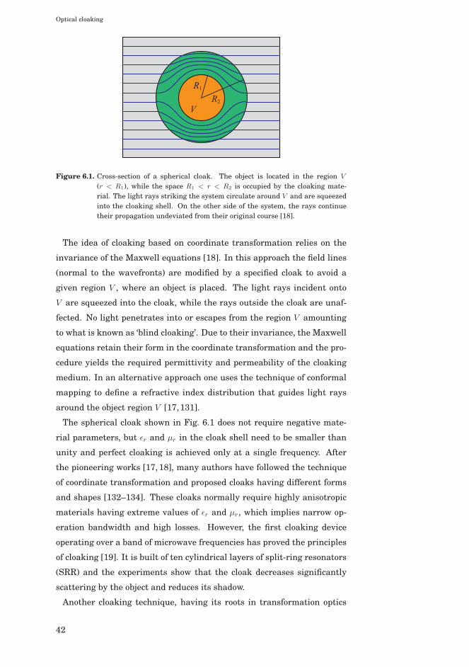
Optical cloaking

R1

R2V

Figure 6.1. Cross-section of a spherical cloak. The object is located in the region V

(r < R1), while the space R1 < r < R2 is occupied by the cloaking mate-rial. The light rays striking the system circulate around V and are squeezedinto the cloaking shell. On the other side of the system, the rays continuetheir propagation undeviated from their original course [18].

The idea of cloaking based on coordinate transformation relies on the

invariance of the Maxwell equations [18]. In this approach the field lines

(normal to the wavefronts) are modified by a specified cloak to avoid a

given region V , where an object is placed. The light rays incident onto

V are squeezed into the cloak, while the rays outside the cloak are unaf-

fected. No light penetrates into or escapes from the region V amounting

to what is known as ‘blind cloaking’. Due to their invariance, the Maxwell

equations retain their form in the coordinate transformation and the pro-

cedure yields the required permittivity and permeability of the cloaking

medium. In an alternative approach one uses the technique of conformal

mapping to define a refractive index distribution that guides light rays

around the object region V [17,131].

The spherical cloak shown in Fig. 6.1 does not require negative mate-

rial parameters, but εr and μr in the cloak shell need to be smaller than

unity and perfect cloaking is achieved only at a single frequency. After

the pioneering works [17, 18], many authors have followed the technique

of coordinate transformation and proposed cloaks having different forms

and shapes [132–134]. These cloaks normally require highly anisotropic

materials having extreme values of εr and μr, which implies narrow op-

eration bandwidth and high losses. However, the first cloaking device

operating over a band of microwave frequencies has proved the principles

of cloaking [19]. It is built of ten cylindrical layers of split-ring resonators

(SRR) and the experiments show that the cloak decreases significantly

scattering by the object and reduces its shadow.

Another cloaking technique, having its roots in transformation optics

42

Optical cloaking

and highly promising to mitigate the disadvantages of earlier designs, is

the carpet cloak [135]. Such structures have been experimentally demon-

strated at microwave frequencies [136] and in the optical range [20, 21].

For instance, a particular carpet cloak involving isotropic dielectric ma-

terial renders a remarkable suppression of scattering from a μm-sized

object within a broad band of near-infrared frequencies [20]. Quite re-

cently, a quasi-three-dimensional optical carpet cloak that decreased sig-

nificantly the scattering from an object for viewing angles up to 60◦, was

fabricated [22].

Besides the cloak designs based on coordinate transformations and con-

formal mappings, a variety of other cloaking approaches and related meth-

ods have been put forward. These include reduction of scattering cross-

section [137, 138], use of embedded arrays of holes and dielectric parti-

cles in metal films [139], and utilization of anomalous resonances [140].

For specific light polarizations even mm- and cm-scale three-dimensional

objects are cloaked in visible light [141]. Most of these techniques are

approximate, narrow-band, or based on strong scatterers. Some cloaking

methods can be categorized as ‘cloaking at distance’. In such a case an in-

visibility cloak can hide an object that is external to the cloak itself. The

cloak, which depends on the object, typically is designed employing the

concept of complementary media [142].

6.2 Optical scattering theory

In general, scattering covers a wide range of phenomena arising from the

interaction of waves or particles with media. We focus on the circum-

stances where the response of matter to an electromagnetic field can be

described by the macroscopic material parameters and assume that the

properties of the scattering medium do not change in time. Let us con-

sider a monochromatic electromagnetic field that propagates in vacuum

and is incident on a medium occupying a volume V (see Fig. 6.2). The

medium is characterized by the dielectric permittivity εr and the mag-

netic permeability μr, and it contains no sources of electromagnetic field.

In this case the wave equation in Eq. (A.17) (see also App. A.5) takes the

form

∇×∇×E(r, ω)− k2(r, ω)E(r, ω) = 0, (6.1)

where k2 = k20n

2(r, ω) = k20εr(r, ω)μr(r, ω), with k0 being the vacuum wave

number and n the refractive index. Using vector identities, Maxwell’s

43

Optical cloaking

equations, and the constitutive relations, Eq. (6.1) can be expressed as

∇2E(r, ω) +∇[(∇εr(r, ω)

εr(r, ω)

)·E(r, ω)

]+ k2(r, ω)E(r, ω) = 0. (6.2)

This equation is valid in any nanophotonic structure as long as it can be

described by macroscopic material parameters. The middle term on the

left-hand side in Eq. (6.2) couples the three orthogonal components of the

electric field.

V

E(i)

E(s)(εr , μr)

Figure 6.2. Electromagnetic field is incident on and scattered from a medium occupying avolume V and characterized by the dielectric permittivity εr and the magneticpermeability μr.

We now assume that the material properties within V vary smoothly

with position. If εr changes so slowly that it is effectively constant over

distances of the order of the wavelength, i.e., |∇εr|λ � εr, the middle term

on the left-hand side of Eq. (6.2) is negligible in comparison with the first

one [45,143]. We then obtain

∇2E(r, ω) + k20n

2(r, ω)E(r, ω) = 0, (6.3)

indicating that the electric field components are decoupled. Hence, under

these conditions scalar theory of optical scattering is sufficient.

Denoting the scalar field by U(r, ω) Eq. (6.3) can be rewritten as [45]

∇2U(r, ω) + k20U(r, ω) = −4πF (r, ω)U(r, ω), (6.4)

where

F (r, ω) =14π

k20[n

2(r, ω)− 1] (6.5)

is the scattering potential of the medium. The function F vanishes outside

the scattering volume V . The field U can always be expressed as a sum

U = U (i) + U (s), where U (i) satisfies Eq. (6.4) with F = 0. The field U (i) is

thus generated by sources at infinity and it can be viewed as the incident

field, whereas U (s) may be regarded as the scattered field (see Fig. 6.2).

The solution of Eq. (6.4) is [45] (cf., App. A.4)

U(r, ω) = U (i)(r, ω) +∫

VF (r′, ω)U(r′, ω)

eik0|r−r′|

|r− r′| d3r′, (6.6)

44

Optical cloaking

where the last term under the integral is the outgoing free-space Green

function. Equation (6.6) is the integral equation of potential scattering; it

is an integral equation for U (s) within the volume V .

According to Eq. (6.6) one can calculate the total field outside the scat-

terer if U (s) in V is known. However, in many practical situations finding

the exact U (s) may be difficult and one has to resort to approximate tech-

niques. In the case of a weak scatterer, whose refractive index according

to Eq. (6.5) is close to that of the surroundings, the total field within the

scatterer can be approximated by the incident field only. Thus, Eq. (6.6)

becomes [45]

U(r, ω) = U (i)(r, ω) +∫

VF (r′, ω)U (i)(r′, ω)

eik0|r−r′|

|r− r′| d3r′. (6.7)

This expression, which is the first term in an iterative series solution for

the scattering problem, is the (first-order) Born approximation. Despite

its simplicity the Born approximation gives reasonable results in many

cases of optical scattering.

6.3 Cloaking in the Born approximation

In Publication V we study cloaking by means of classical scattering the-

ory in the case of weak slab scatterers. We consider a monochromatic

field U (i)(r, ω) propagating in vacuum along the z axis and striking a slab

object, as illustrated in Fig. 6.3 (also Fig. 1 in V). The object is located

between 0 ≤ z ≤ a and it has a z-dependent refractive-index distribution

no(z, ω). The cloak slab is placed at a1 ≤ z ≤ a2, where a1 > a. Our goal is

to determine the refractive index nc(z, ω) for the cloak such that the field

Uc(r, ω) scattered from it cancels exactly the scattered field Uo(r, ω) pro-

duced by the known object. The refractive-index distributions of the object

and the cloak are taken smooth and their contrast with the surroundings

low so that the scalar treatment under the first-order Born approximation

is valid. We therefore consider an object-dependent cloak and the process

can be classified as cloaking at distance.

We express the incident and scattered fields by means of the angular

spectrum representation presented in App. A.6. Cloaking is achieved

when the fields scattered by the object and the cloak cancel each other,

i.e., Uo = −Uc, implying that the total field in the space behind the cloak

or in front of the object is equal to the incident field. The former is referred

to as forward cloaking and the latter as backward cloaking, and they place

45

Optical cloaking

0 a z

object

no

U ( i )

Uo Uo

a1 a2

cloak

nc

Uc Uc

Figure 6.3. Illustration of cloaking in a slab geometry. The field U (i) propagates along thez axis in vacuum and is incident on the object (no, 0 ≤ z ≤ a) and cloak (nc,a1 ≤ z ≤ a2) slabs. The fields scattered by the object and cloak are denotedby Uo and Uc, respectively.

different conditions on the scattering potential of the cloak. These cloak-

ing conditions enable us to derive the required refractive-index distribu-

tion for the cloak slab. For simplicity, the thicknesses of the object and

cloak slabs are taken to be equal.

We show that in the forward direction (observer in the half-space z > a2)

any absorbing, stratified, and weakly scattering object can be cloaked by

a slab consisting either of amplifying (active) ordinary medium or of nega-

tively refractive, absorbing metamaterial. Under the conditions assumed

the cloaking is perfect, occurs for any incident field at all frequencies, and

is independent of the cloak position. Further, the dispersion properties

of the cloak are explicitly specified by the refractive index of the object.

The refractive-index profile of the cloak resembles that of the object im-

plying that no strong cloak scatterers are needed. For backward scatter-

ing (observer in the half-space z < 0) the situation is different. In this

case cloaking does not necessitate the use of amplifying or negative-index

materials, but is possible only for incident fields that are superpositions

of diffraction-free waves (Bessel beams) [144, 145]. Such wavefields are

self-imaging fields which repeat periodically on propagation. In addition,

backward cloaking depends on the position of the cloak and occurs only for

certain values of a1. We emphasize that our findings on slab cloaking do

not contradict the known results on non-scattering scatterers [146,147].

46

7. Conclusions and outlook

The results presented in this thesis show that both metallic and NIM su-

perlenses allow electromagnetic near-field imaging of dipole-like objects

with subwavelength resolution (Publications I–IV). The best image qual-

ity is achieved with a low-absorption slab lens having a good impedance

match with its surroundings (Publications I–II). Near-field interactions

among the objects and the imaging element influence the image quality:

in the immediate vicinity of the slab the dipole–slab interaction prevents

the dipole from radiating adversely influencing the imaging capabilities.

With low-loss NIMs the interaction is weak and of short range, whereas

for silver slabs it is stronger and reaches over the near-field zone. The

dipole emission is also suppressed by dipole–dipole near-field interactions

when the objects are close to the lens or each other, in particular with

molecular objects of small size and high polarizability while the effect is

weak for glass or metallic nanoparticles (Publications III–IV).

In near-field imaging two nearby objects are necessarily correlated as

a result of common excitation and because of their near-field coupling.

Due to the interference subwavelength resolution cannot be achieved if

the object dipoles oscillate mostly parallel with the imaging element. On

the other hand, if the emitters are excited such that their dipole moments

are orthogonal to the slab surface, which can be accomplished by total

internal reflection, resolutions well beyond the conventional diffraction

limit are reached (Publication IV). The imaging capabilities of slightly

lossy NIM superlenses are superior to those of metallic ones.

It is also shown in this thesis that any weakly scattering object can be

perfectly cloaked in the forward direction by an absorbing NIM or ampli-

fying positive-index medium in slab geometry (Publication V). Cloaking

takes place for incident fields of arbitrary spatial structure and spectral

width. In backscattering, cloaking is achievable at least for incident self-

47

Conclusions and outlook

imaging fields. In both forward and backward cloaking, the refractive-

index profile of the cloak slab resembles that of the object implying that

no strong scatterers are needed for cloaking.

The topics investigated in this thesis belong to fascinating, highly top-

ical, but also very demanding research areas of modern optics. During

the last ten years a variety of physical phenomena involved in superlens

imaging and cloaking have been examined in theoretical studies, many

of which have also been demonstrated experimentally. However, the next

milestone of bringing the proposed ideas and concepts into practise, espe-

cially in the optical regime, requires further progress on metamaterials

and nano-scale fabrication techniques. The results in Publications I–II

are in line with earlier theoretical works and experimental demonstra-

tions of near-field superlenses. These papers contain the most detailed

formalism thus far for determining the image-intensity distribution of a

single radiating point dipole, which is not a two-dimensional grating or

structure used in experiments. The interactions are an inherent feature

of nanoscale imaging techniques, but in the context of superlenses they

have not been studied much. Therefore, the investigation on interactions

reported in Publications III–IV provides useful information for the de-

velopment of superlens systems, and are also valuable from the physical

point of view. The research on weak scatterers in Publication V introduces

the principle of cloaking from a new perspective, and thus broadens the

scale of cloaking applications.

Altogether, in this thesis only a limited number of aspects concerning

the research topics could be addressed. In theoretical physics approxi-

mations are made and the results are to be regarded within the realm of

those approximations. Each part of the investigations in this work raises

a number of important questions, many of which remain unanswered.

For instance, could the proposed concepts on slab cloaking be extended to

strongly scattering stratified objects, at least for beam illumination? On

a more fundamental scale, what is the role of spatial dispersion in the

various metamaterial structures and how does it affect near-field imaging

with NIM slabs? Another task would be to include multipole terms into

the scattering model of nanoparticles. Consideration of the polarization

state in the image fields would provide additional information on the ob-

jects under study. In the end, the fidelity of any near-field imaging system

is determined by the images of real objects it produces.

48

Appendix A: Basic tools ofelectromagnetic optics

A.1 Maxwell’s equations

The behavior of an electromagnetic field in any medium is governed by

the Maxwell equations. The macroscopic Maxwell equations in SI units

read as [148]

∇ ·D(r, t) = ρ(r, t), (A.1)

∇ ·B(r, t) = 0, (A.2)

∇×E(r, t) = −∂B(r, t)∂t

, (A.3)

∇×H(r, t) =∂D(r, t)

∂t+ j(r, t), (A.4)

where D denotes the electric displacement, B the magnetic induction, E

the electric field, and H the magnetic field. The sources of the field are the

free charge density ρ and the free current density j. They are considered

as continuous functions in macroscopic electrodynamics.

The above equations are written in the space–time domain, but the elec-

tromagnetic field, and in particular its interaction with matter, are more

easily analyzed in the space–frequency domain. To do this, one can use

the spectral representation of time dependent fields: the spectrum F(r, ω)

of an arbitrary time-dependent field F(r, t) is defined by the Fourier trans-

form. On the other hand, if F(r, ω) is known, the time-dependent field can

be calculated by the inverse Fourier transform [10]

F(r, t) =∫ ∞

−∞F(r, ω)e−iωtdω. (A.5)

Applying the Fourier transform to Eqs. (A.1)–(A.4) one obtains Maxwell’s

49

Appendix A: Basic tools of electromagnetic optics

equations in the space–frequency domain

∇ · D(r, ω) = ρ(r, ω), (A.6)

∇ · B(r, ω) = 0, (A.7)

∇× E(r, ω) = iωB(r, ω), (A.8)

∇× H(r, ω) = −iωD(r, ω) + j(r, ω), (A.9)

which hold for the spectral components of the electromagnetic field.

A.2 Response of matter to electromagnetic fields

An electromagnetic field induces a polarization P and a magnetization M

in the medium. The vectors D and B take into account this response of

matter, and are connected to the polarization and magnetization accord-

ing to the relations [148]

D(r, t) = ε0E(r, t) + P(r, t), (A.10)

B(r, t) = μ0[H(r, t) + M(r, t)], (A.11)

where ε0 and μ0 are the electric permittivity and magnetic permeability

of vacuum, respectively. In general, the relation between E and D (H and

B) can be rather complicated. In this work, I consider the electromagnetic

field in linear, isotropic, stationary, spatially non-dispersive, but tempo-

rally dispersive medium. In that case the polarization and the magneti-

zation are connected to the electric and magnetic field via the following

convolution relations [10,149]

P(r, t) = ε0

∫ t

−∞χe(r, t− t′)E(r, t′)dt′, (A.12)

M(r, t) =∫ t

−∞χm(r, t− t′)H(r, t′)dt′, (A.13)

where the response functions χe and χm, known as the electric and mag-

netic susceptibilities, vanish for t′ > t. The above equations contain a

signature of causality: the polarization and the magnetization at a time

t depend on the electric and magnetic fields at all time instants t′ before

t (origin of temporal dispersion). The medium may also be spatially dis-

persive (non-local medium) in which case the above relations would be

convolutions over the space, as well. The effects of spatial dispersion can

be observed at interfaces between two media or in metallic objects having

size comparable to the mean free path of electrons [10]. However, in many

cases in nanooptics the non-local effects are very weak and can be safely

50


ignored [10]. Applying the Fourier transform to Eqs. (A.10)–(A.13) one

can write the constitutive relations in the space–frequency domain as

D(r, ω) = ε0εr(r, ω)E(r, ω), (A.14)

B(r, ω) = μ0μr(r, ω)H(r, ω), (A.15)

with εr = 1 + χe and μr = 1 + χm being the relative dielectric permittivity

and magnetic permeability of the medium, respectively.

Besides polarization and magnetization the electromagnetic field may

induce currents. The free current density in the material can be divided

into two parts: the conduction current density, jc, induced by an external

field, and the source current density js. The conduction current density

is connected to the electric component of the external field through the

relation [10,149]

jc(r, ω) = σ(r, ω)E(r, ω), (A.16)

where σ is the conductivity of the medium.

A.3 Wave equations

Starting from the Maxwell curl equations (A.3)–(A.4) and using the rela-

tions (A.10)–(A.11) for D and B, one can derive the inhomogeneous wave

equations in the space–time domain for both the electric and magnetic

fields [10]. Correspondingly, using Maxwell’s curl equations (A.8)–(A.9)

with the constitutive relations (A.14)–(A.16) gives the wave equations in

the space–frequency domain [10]

∇×∇× E(r, ω)− k2(r, ω)E(r, ω) = iωμ0μr(r, ω)js(r, ω), (A.17)

∇×∇× H(r, ω)− k2(r, ω)H(r, ω) = ∇× js(r, ω), (A.18)

where k = k0n is the wave number in medium. Here k0 = ω/c0 is the

vacuum wave number with c0 = (ε0μ0)−1/2 being the vacuum speed of

light, and n2 = εrμr denotes the square of the refractive index of the ma-

terial, with the substitution εr +iσ/ωε0 → εr. These wave equations which

describe the propagation of an electromagnetic field are valid also in an

inhomogeneous medium.

A.4 The Green function

The Green function gives the electromagnetic field produced by a point

source in a certain geometry. In a homogeneous (infinite) medium the

51


Green function↔G satisfies the equation [10,25]

∇×∇×↔G(r, r′, ω)− k2(ω)

↔G(r, r′, ω) =

↔Iδ(r− r′), (A.19)

where↔I is the unit tensor and δ denotes the delta function describing the

point current source at r′. A solution of Eq. (A.19) takes the form [10,25]

↔G(r, r′, ω) =

[↔I+

1k2∇∇

]G(r, r′, ω), (A.20)

where

G(r, r′, ω) =eik|r−r′|

4π|r− r′| (A.21)

is the outgoing scalar Green function that satisfies the Helmholtz equa-

tion [10, 25]. In terms of the Green function the solution of Eq. (A.17) for

a current distribution js, located in a volume V , becomes [10,25]

E(r, ω) = E0(r, ω) + iωμ0μr(ω)∫

V

↔G(r, r′, ω) js(r′)d3r′, (A.22)

where r is a point located outside V . The field E0 represents a wave cre-

ated by sources located at infinity.

In nanooptics one is often interested in the electric field generated by

an electric point dipole. For the dipole located at r′ and having the dipole

moment q the current density has the form [10]

js(r) = −iωqδ(r− r′), (A.23)

and the electric field can be calculated by inserting this expression into

Eq. (A.22). If E0 = 0 one ends up with Eq. (2.1).

A.5 Monochromatic fields

A monochromatic (time-harmonic) field oscillates at a single, constant fre-

quency. In reality no wave is strictly monochromatic, but comprises a

band of frequencies. However, any field with an arbitrary time-dependence

can be expressed as a superposition of monochromatic waves. Further,

the temporal dispersion in an optical system can be taken into account

by considering the wave propagation for monochromatic fields at different

frequencies separately. Monochromatic field components at frequency ω

have the form [10]

F(r, t) = F(r, ω)e−iωt, (A.24)

52


where the spatial part F(r, ω) is complex. For the time-harmonic fields

the time-dependent Maxwell equations (A.1)–(A.4) take the form [10]

∇ ·D(r, ω) = ρ(r, ω), (A.25)

∇ ·B(r, ω) = 0, (A.26)

∇×E(r, ω) = iωB(r, ω), (A.27)

∇×H(r, ω) = −iωD(r, ω) + j(r, ω). (A.28)

One can notice that these Maxwell equations are equivalent to those of

the spectral components of an arbitrary time-dependent field (A.6)–(A.9).

Hence, the solutions for E(r, ω) and H(r, ω) are identical to the solutions

for E(r, ω) and H(r, ω).

For dielectric materials the free charge density ρ and the source current

density js are zero. This is valid also for materials having appreciable con-

ductivity, i.e., for metals [45]. If further the medium is homogenous, i.e.,

the material parameters do not depend on r, the wave equations (A.17)–

(A.18) reduce to the homogenous Helmholtz equations [10]

[∇2 + k2(ω)]E(r, ω) = 0, (A.29)

[∇2 + k2(ω)]H(r, ω) = 0. (A.30)

The most common solution for the Helmholtz equations is the monochro-

matic plane wave for which the spatial part of the field has the form

E(r, ω) = E0(ω)eik·r, (A.31)

H(r, ω) = H0(ω)eik·r, (A.32)

where E0(ω) and H0(ω) are the complex electric and magnetic field ampli-

tudes. The vector k is the wave vector having the property

k · k = k20εr(ω)μr(ω), (A.33)

which is known as the dispersion relation.

A.6 Angular spectrum representation

The angular spectrum representation is a useful mathematical technique

for studying the propagation of optical fields in homogenous media [10,38,

143, 150]. One understands the angular spectrum representation as an

expansion of an optical field, in a source-free slab or half-space, in terms

of plane waves with variable amplitudes and propagation directions.

53


Consider a monochromatic field in a slab filling the region 0 ≤ z ≤ Z.

All the sources are located outside the slab, and hence, the spatial part of

the field satisfies the Helmholtz equations (A.29)–(A.30). I assume that

in any plane with constant z inside the slab the field can be expressed as

a Fourier integral

E(x, y, z, ω) =∫∫ ∞

−∞E(kx, ky; z, ω)ei(kxx+kyy)dkxdky, (A.34)

where kx and ky are spatial frequencies corresponding to the Cartesian

transverse coordinates x and y, respectively. Inserting this expression

into the Helmholtz equation gives the differential equation for E(kx, ky; z, ω)

[10,38]∂2E(kx, ky; z, ω)

∂2z+ k2

zE(kx, ky; z, ω) = 0, (A.35)

where

kz = +[k2 − (k2x + k2

y)]1/2, k2

x + k2y ≤ k2, (A.36)

kz = +i[(k2x + k2

y)− k2]1/2, k2x + k2

y > k2, (A.37)

and k = k0n is the wave number within the slab. Using the general so-

lution for the differential equation (A.35) the field in the slab can be ex-

pressed as [10,38]

E(x, y, z, ω) =∫∫ ∞

−∞A(kx, ky; ω)ei(kxx+kyy+kzz)dkxdky

+∫∫ ∞

−∞B(kx, ky; ω)ei(kxx+kyy−kzz)dkxdky, (A.38)

where A(kx, ky; ω) and B(kx, ky; ω) are arbitrary functions. This expres-

sion is known as the angular spectrum representation.

When the refractive index is real and positive, the z component of the

wave vector, kz, is either real or purely imaginary. Therefore, the formula

in Eq. (A.38) represents the wave field in terms of four types of plane-wave

solutions:

(i) ei(kxx+kyy)eikzz, with kz = +[k2 − (k2x + k2

y)]1/2 and k2

x + k2y ≤ k2.

These solutions are homogenous plane waves that propagate from the

boundary plane z = 0 towards the boundary plane z = Z > 0.

(ii) ei(kxx+kyy)eikzz, with kz = +i[k2x + k2

y − k2]1/2 and k2x + k2

y > k2.

These waves are inhomogenous with the amplitudes decaying exponen-

tially from the plane z = 0 towards the plane z = Z > 0. Inhomogeneous

waves of this kind are also known as evanescent waves.

54


(iii) ei(kxx+kyy)e−ikzz, with kz = +[k2 − (k2x + k2

y)]1/2 and k2

x + k2y ≤ k2.

These are homogenous plane waves that propagate from the boundary

plane z = Z > 0 towards the boundary plane z = 0.

(iv) ei(kxx+kyy)e−ikzz, with kz = +i[k2x + k2

y − k2] and k2x + k2

y > k2.

These are evanescent waves and their amplitudes decay exponentially

from the plane z = Z towards the plane z = 0.

One should note that in an absorbing material the permittivity and the

permeability are complex quantities. Consequently, the wave vector be-

comes complex as well, and the waves decay due to absorbtion of the

medium. Thus, I can no longer use the terms propagating and evanes-

cent, but I preferably speak of slowly decaying and fast decaying waves

when I refer to the waves related to low spatial frequencies (propagating)

and high spatial frequencies (evanescent), respectively.

The angular spectrum representation for a field that propagates into the

half-space z ≥ 0 and whose sources are located in z < 0 is obtained from

Eq. (A.38) by neglecting the latter term [38]. The spectral amplitudes

A(kx, ky; ω) of each plane-wave component can be expressed by the Fourier

transform of the field in the plane z = 0. Thus, if the field is known in the

plane z = 0, it is known throughout the half space z > 0 in terms of the

angular spectrum representation.

A.7 Boundary conditions

The boundary conditions for the electromagnetic field at the interface be-

tween two media are conventionally derived from the integral forms of

the Maxwell equations. The boundary conditions are valid for both the

time-dependent fields and their spectral components, and they are of the

form [10]

n× (E2 −E1) = 0, (A.39)

n× (H2 −H1) = jsu, (A.40)

n · (D2 −D1) = ρsu, (A.41)

n · (B2 −B1) = 0, (A.42)

where n is the unit normal vector of the interface pointing from medium

of incidence (medium 1) into medium of transmittance (medium 2). The

vector jsu denotes the surface current density, and ρsu is the surface charge

55


density. The fields on both sides of the interface are connected by Maxwell’s

equations, and hence, the boundary conditions are not independent of

each other. The surface current density, jsu, and the surface charge den-

sity, ρsu, vanish in the case of any real materials because they are not

perfectly conducting [45].

A.8 Fresnel’s coefficients

When light propagates across an interface between two media, reflection

and refraction take place. The Fresnel reflection and transmission coef-

ficients, rs,p and ts,p, respectively, describe how the amplitude and phase

of a plane wave are changed in reflection and transmission. These coef-

ficients are usually derived for s and p polarizations from the boundary

conditions and they read as [10,45,148]

rs(kx, ky, ω) =μr,2(ω)kz,1(ω)− μr,1(ω)kz,2(ω)μr,2(ω)kz,1(ω) + μr,1(ω)kz,2(ω)

, (A.43)

ts(kx, ky, ω) =2μr,2(ω)kz,1(ω)

μr,2(ω)kz,1(ω) + μr,1(ω)kz,2(ω), (A.44)

rp(kx, ky, ω) =εr,2(ω)kz,1(ω)− εr,1(ω)kz,2(ω)εr,2(ω)kz,1(ω) + εr,1(ω)kz,2(ω)

, (A.45)

tp(kx, ky, ω) =2εr,2(ω)kz,1(ω)

εr,2(ω)kz,1(ω) + εr,1(ω)kz,2(ω)

√μr,2(ω)εr,1(ω)μr,1(ω)εr,2(ω)

, (A.46)

where the subscript 1 denotes the medium of incidence and the subscript

2 refers to the medium of transmittance. The Fresnel coefficients are valid

for both the propagating and evanescent waves.

I note that unlike commonly perceived, the Fresnel transmission coeffi-

cient tp in Eq. (A.46) is not, in general, the ratio of the complex amplitude

of the transmitted field to that of the incident field. If the unit vector p

specifying the p-polarized electric field component is complex, which hap-

pens for evanescent fields and when one or both of the media are lossy, p

is not normalized in the sense of complex-valued vectors [41,62].

56

References

[1] V. G. Veselago, “The electrodynamics of substances with simulta-

neously negative values of ε and μ”, Sov. Phys. Usp. 10, 509–514

(1968).

[2] R. Marques, F. Martin, and M. Sorolla, Metamaterials with Nega-

tive Parameters: Theory, Design, and Microwave Applications (Wi-

ley, Hoboken, 2008).

[3] L. Solymar and E. Shamonina, Waves in Metamaterials (Oxford

University Press, New York, 2009).

[4] V. M. Shalaev, “Optical negative-index metamaterials”, Nature Pho-

ton. 1, 41–48 (2007).

[5] C. M. Soukoulis, S. Linden, and M. Wegener, “Negative refractive

index at optical wavelengths”, Science 315, 47–49 (2007).

[6] Y. Liu and X. Zhang, “Metamaterials: a new frontier of science and

technology”, Chem. Soc. Rev. 40, 2494–2507 (2011).

[7] X. Zhang and Z. Liu, “Superlenses to overcome the diffraction limi”,

Nature Mater. 7, 435–441 (2008).

[8] V. M. Shalaev, “Transforming light”, Science 322, 384–386 (2008).

[9] H. Chen, C. T. Chan, and P. Sheng, “Transformation optics and

metamaterials”, Nature Mater. 9, 387–396 (2010).

[10] L. Novotny and B. Hecht, Principles of Nano-Optics (Cambridge

University Press, Cambridge, 2006).

[11] L. Novotny, “The history of near-field optics”, in Progress in Optics,

ed. E. Wolf (Elsevier, Amsterdam, 2007), vol. 50, pp. 137–184.

57

References

[12] D. Courjon, Near-Field Microscopy and Near-Field Optics (Imperial

College Press, London, 2003).

[13] J. B. Pendry, “Negative refraction makes a perfect lens”, Phys. Rev.

Lett. 85, 3966–3969 (2000).

[14] N. Fang, H. Lee, C. Sun, and X. Zhang, “Sub-diffraction-limited

imaging with a silver superlenses”, Science 308, 534–537 (2005).

[15] H. Lee, Y. Xiong, N. Fang, W. Srituravanich, S. Durant, M. Ambati,

C. Sun, and X. Zhang, “Realization of optical superlens imaging be-

low the diffraction limit”, New J. Phys. 7, 255 (2005).

[16] P. Chaturvedi, W. Wu, V. J. Logeeswaran, Z. Yu, M. S. Islam, S. Y.

Wang, R. S. Williams, and N. X. Fang, “A smooth optical superlens”,

Appl. Phys. Lett. 96, 043102 (2010).

[17] U. Leonhardt, “Optical conformal mapping”, Science 312, 1777–

1780 (2006).

[18] J. B. Pendry, D. Schurig, and D. R. Smith, “Controlling electromag-

netic fields”, Science 312, 1780–1782 (2006).

[19] D. Schurig, J. J. Mock, B. J. Justice, S. A. Cummer, J. B. Pendry, A.

F. Starr, and D. R. Smith, “Metamaterial electromagnetic cloak at

microwave frequencies”, Science 314, 977–980 (2006).

[20] J. Valentine, J. Li, T. Zentgraf, G. Bartal, and X. Zhang, “An optical

cloak made of dielectrics”, Nature Mater. 8, 568–571 (2009).

[21] L. H. Gabricelli, J. Cardenas, C. B. Poitras, and M. Lipson, “Sili-

con nanostructure cloak operating at optical frequencies”, Nature

Photon. 3, 461–463 (2009).

[22] T. Ergin, N. Stenger, P. Brenner, J. B. Pendry, and M. Wegener,

“Three-dimensional invisibility cloak at optical wavelengths”, Sci-

ence 328, 337–339 (2010).

[23] M. W McGall, A Farfaro, P. Kinrles, and A. Boardman, “A spacetime

cloak or a history editor”, J. Opt. 13, 024003 (2011).

[24] M. Fridman, A. Farsi, Y. Okawachi, and A. L. Gaeta, “Demonstra-

tion of temporal cloaking”, Nature Lett. 481, 62–65 (2012).

[25] C.-T. Tai, Dyadic Green’s Functions in Electromagnetic Theory (In-

text, Scranton, 1971).

58

References

[26] G. F. Bohren and D. R. Huffman, Absorption and Scattering of Light

by Small Particles (Wiley, New York, 1998).

[27] R. Carminati, J.-J. Greffet, C. Henkel, and J. M. Vigoureux, “Radia-

tive and non-radiative decay of a single molecule close to a metallic

nanoparticle”, Opt. Commun. 261, 368–375 (2006).

[28] M. Fox, Quantum Optics: An Introduction (Oxford University Press,

Oxford, 2006).

[29] J. Grondalski and D. F. V. James, “Is there a fundamental limita-

tion on the measurements of spatial coherence for highly incoherent

fields”, Opt. Lett. 28, 1630–1632 (2003).

[30] O. Keller, M. Xiao, and S. Bozhevolnyi, “Configurational resonances

in optical near-field microscopy: a rigorous point-dipole approach”,

Surf. Sci. 280, 217–230 (1993).

[31] E. M. Purcell and C. R. Pennypacker, “Scattering and absorbtion of

light by nonspherical dielectric grains”, Astrophys. J. 186, 705–714

(1973).

[32] B. T. Draine, “The discrete dipole approximation and its application

to interstellar graphite grains”, Astrophys. J. 333, 848–872 (1988).

[33] B. T. Draine and J. Goodman, “Beyond Clausius-Mossotti: Wave

propagation on a polarizable point lattice and the discrete dipole

approximation”, Astrophys. J. 405, 685–697 (1993).

[34] B. T. Draine and P. J. Flatau, “Discrete-dipole approximation for

scattering calculations”, J. Opt. Soc. Am. A 11, 1491–1499 (1994).

[35] M. A. Yurkin and A. G. Hoekstra, “The discrete dipole approxima-

tion: an overview and recent developments”, J. Quant. Spectrosc.

Radiat. Transfer 106, 558–589 (2007).

[36] M. A. Yurkin and A. G. Hoekstra, “The discrete dipole approxima-

tion code ADDA: Capabilities and known limitations”, J. Quant.

Spectrosc. Radiat. Transfer 112, 2234–2247 (2011).

[37] G. J. Gbur, Mathematical Methods for Optical Physics and Engi-

neering (Cambridge University Press, New York, 2011).

[38] L. Mandel and E. Wolf, Optical Coherence and Quantum Optics

(Cambridge University Press, Cambridge, 1995).

59

References

[39] K.-H. Brenner, “Plane wave decomposition in layered materials and

meta-materials”, in 6th International Workshop on Information Op-

tics (WIO ’07), eds. J. A. Benediktsson, B. Javidi, and K. S. Gudmun-

sson, AIP Conference Proc. 949, 59–66 (2007).

[40] J. E. Sipe, “New Green-function formalism for surface optics”, J.

Opt. Soc. Am. B 4, 481–489 (1987).

[41] A. Norrman, T. Setälä, and A. T. Friberg, “Partial spatial coherence

and partial polarization in random evanescent fields on lossless in-

terfaces”, J. Opt. Soc. Am. A 28, 391–400 (2011).

[42] G. W. ’t Hooft, “Comment on ‘Negative refraction makes a perfect

lens’ ”, Phys. Rev. Lett. 87, 249701 (2001).

[43] J. B. Pendry, “Reply to the comment by G. W. ’t Hooft”, Phys. Rev.

Lett. 87, 249702 (2001).

[44] P. M. Morse and H. Feshbach, Methods of Theoretical Physics

(McGraw-Hill, New York, 1953).

[45] M. Born and E. Wolf, Principles of Optics, 7th ed. (Cambridge Uni-

versity Press, Cambridge, 1999).

[46] P. B. Johnson and R. W. Christy, “Optical constants of the noble

metals”, Phys. Rev. B 6, 4370–4379 (1972).

[47] A. Moroz, “Non-radiative decay of a dipole emitter close to a metallic

nanoparticle: Importance of higher-order multipole contributions”,

Opt. Commun. 283, 2277–2287 (2010).

[48] S. Kawata, Near-Field Optics and Surface Plasmon Polaritons

(Springer, Heidelberg, 2001).

[49] H. Raether, Surface Plasmons on Smooth and Rough Surfaces and

on Gratings (Springer, Berlin, 1988).

[50] S. A. Maier and H. A. Atwater, “Plasmonics: Localization and

guiding of electromagnetic energy in metal/dielectric structures”,

J. Appl. Phys. 98, 011101 (2005).

[51] J. M. Pitarke, V. M. Silkin, E. V. Chulnov, and P. M. Echenique,

“Theory of surface plasmons and surface plasmon polaritons”, Rep.

Prog. Phys. 70, 1–87 (2007).

60

References

[52] D. Sarid and W. Challener, Modern Introduction to Surface Plas-

mons (Cambridge University Press, Cambridge, 2010).

[53] A. V. Zayats, I. I. Smolyaninov, and A. A. Maradudin, “Nano-optics

of surface plasmon polaritons”, Phys. Rep. 408, 131–314 (2005).

[54] P. Berini, “Long-range surface plasmon polaritons”, Adv. Opt. Phot.

1, 484–588 (2009).

[55] C. Genet and T. W. Ebbesen, “Light in tiny holes”, Nature 445, 39–

46 (2007).

[56] S. Lal, S. Link, and N. J. Halas, “Nano-optics from sensing to waveg-

uiding”, Nature Phot. 1, 641–648 (2007).

[57] J. Heber, “Surfing the wave”, Nature 461, 720–722 (2009).

[58] M. Ozaki, J.-I. Kato, and S. Kawata, “Surface-plasmon holography

with white-light illumination”, Science 332, 218–220 (2011).

[59] D. K. Gramotnev and S. I. Bozhevolnyi, “Plasmonics beyond the

diffraction limit”, Nature Photon. 4, 83–91 (2010).

[60] M. I. Stockman, “Nanophotonics: past, present, and glimpse into

future”, Opt. Express 19, 22029–22106 (2011).

[61] S. A. Ramakrishna, “Physics of negative refractive index materials”,

Rep. Prog. Phys. 68, 449–521 (2005).

[62] L. D. Landau and E. M. Lifshitz, Electrodynamics of Continuous

Media, 2nd ed. (Pergamon Press, Oxford, 1981).

[63] J. B. Pendry, A. J. Holden, D. J. Robbins, and W. J. Stewart,

“Magnetism from conductors and enhanced nonlinear phenomena”,

IEEE Trans. Microwave Theory Tech. 47, 2075–2084 (1999).

[64] D. R. Smith, W. J. Padilla, D. C. Vier, S. C. Nemat-Nasser, and S.

Schultz, “Composite medium with simultaneously negative perme-

ability and permittivity”, Phys. Rev. Lett. 84, 4184–4187 (2000).

[65] L. V. Panina, A. N. Grigorenko, and D. P. Makhnovskiy, “Optomag-

netic composite medium with conducting nanoelement”, Phys. Rev.

B 66, 155411 (2002).

[66] A. Ishikawa, T. Tanaka, and S. Kawata, "Negative magnetic per-

meability in the visible light region", Phys. Rev. Lett. 95, 237401

(2005).

61

References

[67] M. Kafesaki, I. Tsiapa, N. Katsarakis, Th. Koschny, C. M. Souk-

oulis, and E. N. Economou, “Left-handed metamaterials: The fish-

net structure and its variations”, Phys. Rev. B 75, 235114 (2007).

[68] D. R. Smith, S. Schultz, P. Markos, and C. M. Soukoulis, “Deter-

mination of effective permittivity and permeability of metamateri-

als from reflection and transmission coefficients”, Phys. Rev. B 65,

195104 (2002).

[69] D. R. Smith, D. C. Vier, Th. Koschny, and C. M. Soukoulis, “Electro-

magnetic parameter retrieval from inhomogeneous metamaterials”,

Phys. Rev. E 71, 036617 (2005).

[70] C. Menzel, T. Paul, C. Rockstuhl, T. Pertsch, S. Tretyakov, and F.

Lederer, “Validity of effective material parameters for optical fish-

net metamaterials”, Phys. Rev. B 81, 035320 (2010).

[71] R. A. Shelby, D. R. Smith, and S. Schultz, “Experimental verification

of a negative index of refraction”, Science 292, 77–79 (2001).

[72] C. G. Parazzoli, R. B. Greegor, K. Li, B. E. C. Koltenbah, and M.

Tanielian, “Experimental verification and simulation of negative

index of refraction using Snell’s law”, Phys. Rev. Lett. 90, 107401

(2003).

[73] T. J. Yen, W. J. Padilla, N. Fang, D. C. Vier, D. R. Smith, J. B. Pendry,

D. N. Basov, and X. Zhang, "Terahertz magnetic response from arti-

ficial materials”, Science 303, 1494–1496 (2004).

[74] S. Linden, C. Enkrich, M. Wegener, J. Zhou, T. Koschny, C. M. Souk-

oulis, “Magnetic response of metamaterials at 100 terahertz”, Sci-

ence 306, 1351–1353 (2004).

[75] S. Zhang, W. Fan, B. K. Minhas, A. Frauenglass, K. J. Malloy, and

S. R. J. Brueck, “Midinfrared resonant magnetic nanostructures

exhibiting a negative permeability”, Phys. Rev. Lett. 94, 037402

(2005).

[76] C. Enkrich, M. Wegener, S. Linden, S. Burger, L. Zschiedrich,

F. Schmidt, J. F. Zhou, T. Koschny, and C. M. Soukoulis, “Mag-

netic metamaterials at telecommunication and visible frequencies”,

Phys. Rev. Lett. 95, 203901 (2005).

62

References

[77] J. Zhou, Th. Koschny, M. Kafesaki, E. N. Economou, J. B. Pendry,

and C. M. Soukoulis, “Saturation of the magnetic response of split-

ring resonators at optical frequencies”, Phys. Rev. Lett. 95, 223902

(2005).

[78] S. Tretyakov, “On geometrical scaling of split-ring and double-bar

resonators at optical frequencies”, Metamaterials 1, 40-43 (2007).

[79] V. M. Shalaev, W. Cai, U. K. Chettiar, H.-K. Yuan, A. K. Sarychev,

V. P. Drachev, and A. V. Kildishev, “Negative index of refraction in

optical metamaterials”, Opt. Lett. 30, 3356–3358 (2005).

[80] G. Dolling, C. Enkrich, M. Wegener, J. F. Zhou, C. M. Soukoulis, and

S. Linden, “Cut-wire pairs and plate pairs as magnetic atoms for

optical metamaterials”, Opt. Lett. 30, 3198–3200 (2005).

[81] A. Ishikawa, T. Tanaka, and S. Kawata, “Magentic excitation of

magnetic resonance in metamaterials at far-infrared frequencies”,

Appl. Phys. Lett. 91, 113118 (2007).

[82] J. Yao, Z. Liu, Y. Liu, Y. Wang, C. Sun, G. Bartal, A. M. Stacy,

and X. Zhang, “Optical negative refraction in bulk metamaterials

of nanowires”, Science 321, 930 (2008).

[83] G. Dolling, C. Enkrich, M. Wegener, C. M. Soukoulis, and S. Linden,

“Simultaneous negative phase velocity of light in a metamaterial”,

Science 312, 892–894 (2006).

[84] G. Dolling, M. Wegener, C. M. Soukoulis, S. T. Linden, “Negative-

index at 780 nm wavelength”, Opt. Lett. 32, 53–55 (2007).

[85] U. K. Chettiar, A. V. Kildishev, H. K. Yuan, W. Cai, S. Xiao, V. P.

Drachev, V. M. Shalaev, “Dual-band negative index metamaterial:

double negative at 813 nm and single negative at 772 nm”, Opt.

Lett. 32, 1671–1673 (2007).

[86] J. Valentine, S. Zhang, T. Zentgraf, E. Ulin-Avila, D. A. Genov,

G. Bartal, and X. Zhang, “Three-dimensional optical metamaterial

with a negative refractive index”, Nature 455, 376–379 (2008).

[87] S. M. Xiao, U. K. Chettiar, A. V. Kildishev, V. P. Drachev, and V.

M. Shalaev, “Yellow-light negative-index metamaterials”, Opt. Lett.

34, 3478–3480 (2009).

63

References

[88] J. Valentine, S. Zhang, T. Zentgraf, and X. Zhang, “Development

of bulk optical negative index fishnet metamaterials: Achieving a

low-loss and broadband response through coupling”, Proc. IEEE 99,

1682–1690 (2011).

[89] S. A. Ramakrishna and J. B. Pendry, “Removal of absorption and

increase in resolution in a near-field lens via optical gain”, Phys.

Rev. B 67, 201101(R) (2003).

[90] A. Xiao, V. P. Drachev, A. V. Kildishev, X. Ni, U. K. Chettiar, H-

K. Yuan, and V. M. Shalaev, “Loss-free and active optical negative-

index metamaterials”, Nature 466, 735–738 (2010).

[91] S. Tretyakov, I. Nefedov, A. Sihvola, S. Maslovski, and C. Simovski,

“Wave and energy in chiral nihility”, J. Electromagn. Waves Appl.

17, 695–706 (2003).

[92] J. B. Pendy, “A chiral route to negative refaction”, Science 306,

1353–1355 (2004).

[93] S. Zhang, Y.-S. Park, J. Li, X. Lu, W. Zhang, and X. Zhang, “Nega-

tive refractive index in chiral metamaterials”, Phys. Rev. Lett. 102,

023901 (2009).

[94] M. J. Huttunen, G. Bautista, M. Decker, S. Linden, M. Wegener, and

M. Kauranen, “Nonlinear chiral imaging of subwavelength-sized

twisted-cross gold nanodimers”, Opt. Mat. Exp. 1, 46–56 (2011).

[95] A. J. Hoffman, L. Alekseyev, S. S. Howard, K. J. Franz, D. Wasser-

man, V. A. Podolskiy, E. E. Narimanov, D. L. Sivco, and C. Gmachl,

“Negative refraction in semiconductor metamaterials”, Nature Mat.

6, 946–950 (2007).

[96] P-Y. Chen, M. Farhat, and A. Alu, “Bistable and self-tunable

negative-index metamaterial at optical frequencies”, Phys. Rev.

Lett. 106, 105503 (2011).

[97] S. A. Ramakrishna and O. J. F. Martin, “Resolving the wave vec-

tor in negative refractive index media”, Opt. Lett. 30, 2626–2628

(2005).

[98] M. C. K. Wiltshire, J. B. Pendry, I. R. Young, D. J. Larkman, D. J.

Gilderdale, and J. V. Hajnal, “Microstructured magnetic materials

64

References

for RF flux guides in magnetic resonance imaging”, Science 291,

849–851 (2001).

[99] A. Alu and N. Engheta, “Guided modes in a waveguide filled with

a pair of single-negative (SNG), double-negative (DNG), and/or

double-positive (DPS) layers”, IEEE Trans. Microwave Theory

Tech. 52, 199–210 (2004).

[100] C. Caloz, A. Sanada, and T. Itoh, “A novel composite right-/left-

handed coupled-line directional coupler with arbitrary coupling

level and broad bandwidth”, IEEE Trans. Microwave Theory Tech.

52, 980–992 (2004).

[101] A. Kurs, A. Karalis, R. Moffatt, J. D. Joannopoulos, P. Fisher, and

M. Soljacic, “Wireless power transfer via strongly coupled magnetic

resonances”, Science 317, 83–86 (2007).

[102] H.-T. Chen, J. F. O’hara, A. K. Azad, A. J. Taylor, R. D. Averitt, D. B.

Shrekenhamer, and W. J. Padilla, “Experimental demonstration of

frequency-agile terahertz metamaterials”, Nature Photon. 2, 295–

298 (2008).

[103] N. I. Landy, S. Sajuyigbe, J. J. Mock, D. R. Smith, and W. J.

Padilla, “Perfect metamaterial absorber”, Phys Rev. Lett. 100,

207402 (2008).

[104] B. Richards and E. Wolf, “Electromagnetic diffraction in optical sys-

tems — II. Structure of the focal region”, Prog. Roy. Soc. A 253,

358–379 (1959).

[105] W. T. Welford, Aberrations of Optical Systems (Taylor & Francis,

New York, 1986).

[106] C. J. R. Sheppard and T. Wilson, “The image of a single point in mi-

croscopes of large numerical aperture”, Proc. Roy. Soc. A 379, 145–

158 (1982).

[107] J. Enderlein, “Theoretical study of detection of a dipole emitter

through an objective with high numerical aperture”, Opt. Lett. 25,

634–636 (2000).

[108] J. W. Goodman, Introduction to Fourier Optics, 3rd ed. (Roberts &

Company, Englewood, 2005).

65

References

[109] J. M. Williams, “Comment on ‘Negative refraction makes a perfect

lens’ Some problems with negative refraction”, Phys. Rev. Lett. 87,

249703 (2001).

[110] J. Pendry, “Reply to the comment by J. M. Williams”, Phys. Rev.

Lett. 87, 249704 (2001).

[111] N. Garcia and M. Nieto-Vesperinas, “Left-handed materials do not

make a perfect lens”, Phys. Rev. Lett. 88, 207403 (2002).

[112] J. Pendry, “Comment on ‘Left-handed materials do not make a per-

fect lens’ ”, Phys. Rev. Lett. 91, 099701 (2003).

[113] M. Nieto-Vesperinas and N. Garcia, “Reply to the comment by J.

Pendry”, Phys. Rev. Lett. 91, 099702 (2003).

[114] M. Nieto-Vesperinas, “Problem of image superresolution with a

negative-index slab”, J. Opt. Soc. Am. A 21, 491–498 (2004).

[115] J. T. Shen and P. M. Platzman, “Near field imaging with negative

dielectric constant lenses”, Appl. Phys. Lett. 80, 3286–3288 (2002).

[116] D. R. Smith, D. Shurig, M. Rosenbluth, S. Schultz, S. A. Ramakr-

ishna, and J. Pendry, “Limitations on subdiffraction imaging with

a negative refractive index slab”, Appl. Phys. Lett. 82, 1506–1508

(2003).

[117] I. A. Larkin and M. I. Stockman, “Imperfect perfect lens”, Nano

Lett. 5, 339–343 (2005).

[118] V. A. Podolskiy and E. E. Narimanov, “Near-sighted superlens”, Opt.

Lett. 30, 75–77 (2005).

[119] V. A Podolskiy, N. A. Kuhta, and G. W. Milton, “Optimizing the su-

perlens: manipulating geometry to enhance the resolution”, Appl.

Phys. Lett. 87, 231113 (2005).

[120] Z. Liu, N. Fang, T.-J. Yen, and X. Zhang, “Rapid growth of evanes-

cent wave by silver superlens”, Appl. Phys. Lett. 83, 5184–5186

(2003).

[121] A. Giannattasio, I. R. Hooper, and W. L. Barnes, “Transmission of

light through thin silver films via surface plasmon-polaritons”, Opt.

Express 12, 5881–5886 (2004).

66

References

[122] A. A. Houck, J. B. Brock, and I. L. Chuang, “Experimental observa-

tions of a left-handed material that obeys Snell’s law”, Phys. Rev.

Lett. 90, 137401 (2003).

[123] A. Grbic and G. V. Eleftheriades, “Overcoming the diffraction limit

with a planar left-handed transmission-line lens”, Phys. Rev. Lett.

92, 117403 (2004).

[124] A. N. Lagarkov and V. N. Kissel, “Near-perfect imaging in a focusing

system based on a left-handed material plate”, Phys. Rev. Lett. 92,

077401 (2004).

[125] T. Taubner, D. Korobkin, Y. Urzhumov, G. Shevts, and R. Hillen-

brand, “Near-field microscopy through a SiC superlens”, Science

313, 1595 (2006).

[126] S. Durant, Z. Liu, J. M. Steele, and X. Zhang, “Theory of the trans-

mission properties of an optical far-field superlens for imaging be-

yond the diffraction limit”, J. Opt. Soc. Am. B 23, 2383–2392 (2006).

[127] J. B. Pendry, “Perfect cylindrical lenses”, Opt. Express 11, 755–760

(2003).

[128] Y. Xiong, Z. Liu, C. Sun, and X. Zhang, “Two-dimensional imaging

by far-field superlens at visible wavelengths”, Nano Lett. 7, 3360–

3365 (2007).

[129] Z. Liu, H. Lee, Y. Xiong, C. Sun, X. Zhang, “Far-field optical hyper-

lens magnifying sub-diffraction-limited objects”, Science 315, 1686

(2007).

[130] P. C. Chaumet, A. Rahmani, F. de Fornel, and J.-P. Dufour, “Evanes-

cent light scattering: The validity of the dipole approximation”,

Phys. Rev. B 58, 2310–2315 (1998).

[131] U. Leonhardt and T. Tyc, “Broadband invisibility by non-euclidean

cloaking”, Science 323, 110–112 (2009).

[132] W. Yan, M. Yan, Z. Ruan, and M. Qiu, “Coordinate transformations

make perfect invisibility cloaks with arbitrary shape”, New J. Phys.

10, 043040 (2008).

[133] A. Nicolet, F. Zolla, and S. Guenneau, “Electromagnetic analysis of

cylindrical cloaks of an arbitrary cross section”, Opt. Lett. 33, 1584–

1586 (2008).

67

References

[134] H. Ma, S. Qu, Z. Xu, and J. Wang, “Numerical method for designing

approximate cloaks with arbitrary shapes”, Phys. Rev. E 78, 036608

(2008).

[135] J. Li and J. B. Pendry, “Hiding under the carpet: a new strategy for

cloaking”, Phys. Rev. Lett. 101, 203901 (2008).

[136] H. F. Ma and T. J. Cui, “Three-dimensional broadband ground-plane

cloak made of metamaterials”, Nature Commun. 1, 1–6 (2010).

[137] M. G. Silverinha, A. Alu, and N. Engheta, “Parallel-pate metamate-

rials for cloaking structures”, Phys. Rev. E 75, 036603 (2007).

[138] S. Tretyakov, P. Alitalo, O. Luukkonen, and C. Simovski, “Broad-

band electromagnetic cloaking of long cylindrical objects”, Phys.

Rev. Lett. 103, 103905 (2009).

[139] F. J. Garcia de Abajo, G. Gomez-Santos, L. A. Blanco, A. G. Borisov,

and S. V. Shabanov, “Tunneling mechanism of light transmission

through metallic films”, Phys. Rev. Lett. 95, 067403 (2005).

[140] N.-A. P. Nicorovici, G. W. Milton, R. C. McPhedran, L. Botten, “Qua-

sistatic cloaking of two-dimensional polarizable discrete systems by

anomalous resonance”, Opt. Express 15, 6314-6323 (2007).

[141] X. Chen, Y. Luo, J. Zhang, K. Jiang, J. B. Pendry, and S. Zhang,

“Macroscopic invisibility cloaking of visible light”, Nature Commun.

2, 1–6 (2011).

[142] Y. Lai, H. Chen, Z.-Q. Zhang, and C. T. Tan, “Complementary me-

dia invisibility cloak that cloaks objects at a distance outside the

cloaking shell”, Phys. Rev. Lett. 102, 093901 (2009).

[143] M. Nieto-Vesperinas, Scattering and Diffraction in Physical Optics

(Wiley, New York, 1991).

[144] A. Hakola, T. Hakkarainen, R. Tommila, and T. Kajava, “Energetic

Bessel-Gauss pulses from diode-pumped solid-state lasers”, J. Opt.

Soc. Am. B 27, 2342–2349 (2010).

[145] J. Turunen and A. T. Friberg, “Propagation-invariant optical fields”,

in Progress in Optics, ed. E. Wolf (Elsevier, Amsterdam, 2009), vol.

54, pp. 1–88.

68

References

[146] G. Gbur, “Nonradiating sources and other invisible objects”, in

Progress in Optics, ed. E. Wolf (Elsevier, Amsterdam, 2003), vol.

45, pp. 273–315.

[147] B. J. Hoenders, “The uniqueness of inverse problems”, in Inverse

Source Problems in Optics, ed. H. P. Baltes (Springer, Berlin, 1978),

pp. 41–82.

[148] J. D. Jackson, Classical Electrodynamics, 3rd ed. (Wiley, New York,

1999).

[149] T. B. Hansen and A. D. Yaghjian, Plane-Wave Theory of Time-

Domain Fields (IEEE Press, New York, 1999).

[150] M. Fertig and K.-H. Brenner, “Vector wave propagation method”, J

Opt. Soc. Am A 27, 709–717 (2010).

69

References

70

Errata

Publication I

There are misprints in Eqs. (26), (27), and (29). On the right-hand side of

these equations the minus signs in front of the brackets should be located

right after the equal signs.

71

Errata

72

9HSTFMG*aeigia+

Documents

W ()*).)(# - W /* ,& (- W ' !#(! W) W #*)& , W '#.. ,- Wlib.tkk.fi/Diss/2012/isbn9789526048697/isbn9789526048697.pdf · Abstract Aalto University, P.O. Box 11000, FI-00076 Aalto Author

W ()).)(# - W / ,& (- W ' !#(! W) W #*)& , W '#.. ,- Wlib.tkk.fi/Diss/2012/isbn9789526048697/isbn9789526048697.pdf · Abstract Aalto University, P.O. Box 11000, FI-00076 Aalto Author