W ATER MANAGEMENT IN REFINERIES - University of Oklahoma

WATER MANAGEMENT IN

REFINERIES

UNIVERSITY OF OKLAHOMA DEPARTMENT OF CHEMICAL , B IOLOGICAL , AND M ATERIALS

ENGINEERING

APRIL 30, 2007

M. COL IN A RNOLD JOS HI SAM UEL

2

TABLE OF CONTENTS

E X E C U T I V E S U M M A R Y ............................................................................................. 5

I. I N T R O D U C T I O N ....................................................................................................... 6

I I . P R O B L E M S T A T E M E N T ...................................................................................... 6

I I I . B A C K G R O U N D ...................................................................................................... 7

1. PROCESS UNITS .......................................................................................................... 7

2 . W A T E R T R E A T M E N T ........................................................................................... 13

3. C O N C E N T R A I O N R A T I N G S O F U N I T S ...................................................... 19

V. R E S U L T S ............................................................................................................... 21

1 . V E R S I O N 0 ................................................................................................................... 22

2 . V E R S I O N 1 ................................................................................................................... 27

3 . V E R S I O N 2 ................................................................................................................... 30

4 . V E R S I O N 3 ................................................................................................................... 34

5 . V E R S I O N 4 ................................................................................................................... 36

6 . R O B U S T N E S S A N A L Y S I S ................................................................................... 42

V . C O N C L U S I O N S ................................................................................................ 46

V I . F U T U R E W O R K A N D R E C O M M E N D A T I O N S ............................ 47

R E F E R E N C E S ......................................................................................................... 48

A P P E N D I C E S ........................................................................................................... 49

A P P E N D I X A : GAMS MODELS .................................................................................... 49

A P P E N D I X B : GAMS SCENARIOS ............................................................................... 72

A P P E N D I X C : PIPING NETWORK BLOCK DIAGRAMS........................................... 74

3

LISTS OF FIGURES, TABLES, AND EQUATIONS

FIGURES

Figure 1: Caustic treating system process flow diagrams4 ............................................................................ 8 Figure 2: Atmospheric distillation operation schematic and process flow diagram3..................................... 9 Figure 3: Vacuum distillation process flow diagram3.................................................................................. 10 Figure 4: Merox-I sweetening process flow diagram3 ................................................................................. 11 Figure 5: Hydrotreating system process flow diagram3,4............................................................................. 12 Figure 6: Desalting unit process flow diagram3,4......................................................................................... 13 Figure 7: API Separator6 ............................................................................................................................. 16 Figure 8: API separator operations diagram6 ............................................................................................. 16 Figure 9: Operation schematic of reverse osmosis (RO) system9 ................................................................ 17 Figure 10: Chevron waste water treatment process flow diagram10............................................................ 18

TABLES

Table 1: Contaminant specifications for each water using unit1.................................................................... 7 Table 2: Water contaminants5 ...................................................................................................................... 14 Table 3: Treatment options for water contaminants5 ................................................................................... 15 Table 4: Flow rates of streams in tons per hour from a unit or fresh water source to another unit or waste water sink as determined by the Version 1 GAMS model............................................................................. 28 Table 5: Flow rates of streams in tons per hour from a unit or fresh water source to another unit or waste water sink as determined in literature1......................................................................................................... 29 Table 6: Flow rates of streams in tons per hour from a unit or fresh water source to another unit or waste water sink as determined by Version 2. ........................................................................................................ 33 Table 7: Flow rates of streams in tons per hour from a unit or fresh water source to another unit or waste water sink as determined by Version 3 ......................................................................................................... 35 Table 8: Flow rates of streams in tons per hour from a unit, regenerator, or fresh water source to another unit or regenerator, or the waste water sink as described by Version 4. ..................................................... 41 Table 9: Flow rates of streams in tons per hour from a unit or fresh water source to another unit or waste water sink as determined by Version 3 under Scenario 1 conditions ........................................................... 42 Table 10: Flow rates of streams in tons per hour from a unit or fresh water source to another unit or waste water sink determined by the modified Version 2 not under Scenario 2 conditions..................................... 44 Table 11: Flow rates of streams in tons per hour from a unit or fresh water source to another unit or waste water sink determined by the modified Version 2 under Scenario 2 conditions........................................... 45

EQUATIONS

Equation 1 .................................................................................................................................................... 20 Equation 2 .................................................................................................................................................... 23 Equation 3 .................................................................................................................................................... 23 Equation 4 .................................................................................................................................................... 24 Equation 5 .................................................................................................................................................... 24 Equation 6 .................................................................................................................................................... 25 Equation 7 .................................................................................................................................................... 25 Equation 8 .................................................................................................................................................... 25 Equation 9 .................................................................................................................................................... 26 Equation 10 .................................................................................................................................................. 26 Equation 11 .................................................................................................................................................. 26 Equation 12 .................................................................................................................................................. 28 Equation 13 .................................................................................................................................................. 31 Equation 14 .................................................................................................................................................. 32 Equation 15 .................................................................................................................................................. 37

4

Equation 16 .................................................................................................................................................. 38 Equation 17 .................................................................................................................................................. 38 Equation 18 .................................................................................................................................................. 39 Equation 19 .................................................................................................................................................. 39 Equation 20 .................................................................................................................................................. 40 Equation 21 .................................................................................................................................................. 40 Equation 22 .................................................................................................................................................. 40 Equation 23 .................................................................................................................................................. 41 Equation 24 .................................................................................................................................................. 41

5

E X E C U T I V E S U M M A R Y Industrial use of water has a long history of maximum use of fresh water input and maximum discharge. Utilizing mathematical algorithms in the GAMS interface, it was shown that a piping network designed for water reuse can be optimized that reduces this fresh water input to a global minimum. Similar studies were first being investigated in the early 1980s; at the same time, industries began focusing on reusing water as a means to increase profit. This study verifies the appropriateness of the use of models in an interface such as GAMS in furthering endeavors to minimize fresh water consumption. This topic recently has become of great interest because of water shortages. In addition, the fresh water purchase costs have led the industries to re-evaluate their strategies. Furthermore, stricter EPA (Environmental Protection Agency) regulations have forced them to optimize their water usage and treatment networks. The mathematical algorithms used in the GAMS interface optimize the water network for a refinery which operates six water using units. Values are assigned to the units as inherent parameters. These parameters include the maximum inlet and outlet concentrations in the water stream, and the process mass loads of the contaminants. Four different algorithms were investigated in the study. Results are compared to values presented in a previous study and these results indicate a wide range of use for the algorithms. An algorithm is written to verify the basic use of the models, two are written to incorporate a minimum flow rate standard, and a last model is written to incorporate regeneration into the system. Finally, robustness studies are carried out to verify the models’ flexibility.

6

I. I N T R O D U C T I O N

For millennia, water has been a fundamental element which has shaped the earth’s

evolution. Life on earth is dependent on water and its cycles which regulate the planet’s

natural processes. Today, water is used for commercial, domestic, industrial, irrigation,

livestock, mining, public supply, and thermoelectric power processes.

Refineries, which are part of the industrial category, use water for many

applications. These applications include stripping, washing, absorption, sweetening, and

other similar processes. Traditionally, fresh water was used for all of these processes

with no reuse or recycling. The processed water was collected into a sink, treated, and

discharged; this collection and treatment process is commonly known as end of pipe

treatment. However, due to stricter EPA (Environmental Protection Agency) regulations,

water scarcity, and the cost of fresh water, industries have focused on alternative

solutions. Beginning in the 1980s, industries started minimizing the fresh water

consumption by reusing process water. They were also interested in ways to recycle

streams with minimum treatment. These prior works provide the motivation for this

investigation.

I I . P R O B L E M S T A T E M E N T

Given a set of water using units and a set of water treatment units, it is desired to

reduce the fresh water intake and total operation cost by maximizing water reuse,

minimizing water discharge, and optimizing the water treatment network1.

7

I I I . B A C K G R O U N D

1. PROCESS UNITS

Six units are chosen to be part of the modeled system1. They are caustic treating,

distillation, amine sweetening, merox-I sweetening, hydrotreating, and desalting units.

Salts, organics, hydrogen sulfide (H2S), and ammonia are the four contaminants

transferred to the water stream in each process. Table 1, shown below, lists maximum

inlet and outlet concentrations and the mass loads ratings associated with each unit.

Contaminant

Salts 300 500 0.18

Organics 50 500 1.2

H2S 5000 11000 0.75

Ammonia 1500 3000 0.1

Salts 10 200 3.61

Organics 1 4000 100

H2S 0 500 0.25

Ammonia 0 1000 0.8

Salts 10 1000 0.6

Organics 1 3500 30

H2S 0 2000 1.5

Ammonia 0 3500 1

Salts 100 400 2

Organics 200 6000 60

H2S 50 2000 0.8

Ammonia 1000 3500 1

Salts 85 350 3.8

Organics 200 1800 45

H2S 300 6500 1.1

Ammonia 200 1000 2

Salts 1000 9500 120

Organics 1000 6500 480

H2S 150 450 1.5

Ammonia 200 400 0

(6) Desalter

(4) Merox I Sweetening

(5) Hydrotreating

(2) Distillation

(3) Amine Sweetening

(ppm) (ppm) (kg/h)

(1) Caustic Treating

Process Cin,max Cout,max Mass Load

Table 1: Contaminant specifications for each water using unit1

8

Caustic treating is a process of removing hydrogen sulfide and ammonia from the

light crude. As shown in the process flow diagram below, the process begins with crude

oil being fed into a distillation column, where components are separated. Hydrogen

sulfide and ammonia exit the column with the gaseous components. Aqueous sodium

hydroxide is used to remove both hydrogen sulfide and ammonia using an absorption

process. The resulting product is a treated light crude component. Figure 1 shows the

schematic of this process.

Figure 1: Caustic treating system process flow diagrams4

Distillation is an integral process that separates crude oil into its many

components. Refineries typically use two types of distillation processes: atmospheric and

vacuum distillation. Crude oil is first fed into the atmospheric distillation column where

at least four side streams are removed from different trays. The light component and

heavy key in each side stream are in equilibrium. Thus, each side stream is sent to a

stripping unit which uses steam to remove the light component. Then, the steam and the

light component are fed back into the atmospheric distillation column above the location

9

of the corresponding side stream. The steam exits the column with the lightest

components, at which point a partial condenser is used to separate the water. The outlet

water stream contains some organics and is sent away for treatment. Figure 2, below,

illustrates the water use in atmospheric distillation.

Figure 2: Atmospheric distillation operation schematic and process flow diagram3

Although atmospheric distillation is very useful in separating the crude oil

components it cannot separate the heaviest organics; they require high vapor pressure for

phase change. Therefore, a vacuum distillation column is used to separate these heavy

components that exit the bottom of the atmospheric distillation column. In this column,

super heated steam is supplied to decrease the vapor pressure and to increase the

10

volatility of the components. Once the lighter components change into the vapor phase,

they are sent to a partial condenser to separate the steam from the organics. Soluble and

emulsified organics remain in the outlet water stream, which is then sent to further

treatment. The process flow diagram for the vacuum distillation is shown in Figure 3.

Feed from atmospheric

Distillation Column

Heavy Component

Steam

Partial Condensor

Light Component

Steam with some

Heavy Organics

Figure 3: Vacuum distillation process flow diagram3

In the sweetening process, the foul odor is removed and the color of the fuel is

improved. The primary cause of foul odor and undesirable color is the presence of

hydrogen sulfide, ammonia, and organo-sulfur compounds. All of these contaminants are

removed using amine and merox-I sweetening processes. The merox-I sweetening

11

process is primarily used for butane and light propane gases, while the amine sweetening

is used for gasoline. Both amine and merox-I sweetening units absorb the acid gases

from the sour gas and send them to a stripper. Steam is used to strip the acidic gases

from the amine and merox-I systems in a stripping unit. The stripped amine and merox-I

absorbents are recycled back for absorption. This process is illustrated in Figure 4 shown

below.

Figure 4: Merox-I sweetening process flow diagram3

The sour feed used in sweetening is first hydrotreated. This is a process used to

remove sulfur, oxygen, nitrogen, halides, and trace metal impurities. It converts most of

the olefins and diolefins into paraffins. The process is initiated by addition of preheated

hydrogen gas into the crude oil. A high pressure reactor is used to produce hydrogen

sulfide and ammonia by reacting the hydrogen with the impurities; if halides and metals

are present, they will form acids and metal hydrides, respectively, though these are not of

interest to the system under investigation. After the reaction, a high pressure membrane

separator is used to recycle any excess hydrogen. The exit stream is composed of a low

12

pressure fuel gas, rich with hydrogen sulfide and ammonia, and the crude liquid contains

dissolved hydrogen sulfide, ammonia and other impurities. The low pressure fuel gas

from this stream is sent to amine and merox-I sweetening units and the liquid stream is

stripped using steam to remove the contaminants. A partial condenser is used to liquefy

all of the steam and the gas stream is mixed with the previously mentioned low pressure

fuel gas as shown in Figure 5.

Figure 5: Hydrotreating system process flow diagram3,4

One of the first processes in any refining operation is a desalting process. This

process is primarily used to remove salts from the unrefined crude. The process begins

with the addition of water to the crude feed stream. The mixture is heated to aid the salts

in aqueous dissolution. A gravity tank is used to allow the water with the salts to settle to

the bottom where it is drained out. The desalted crude is pumped to a distillation column

where further crude treatment is performed. Figure 6 below shows the desalting process.

13

Figure 6: Desalting unit process flow diagram3,4

2 . WATER TREATMENT

There are many types of contaminants that could be present in water. Waste

water contaminants are classified into roughly five different categories. They are

suspended solids, dissolved organics, dissolved salts, microorganisms, and gases. Table

2, shown below, lists these categories with examples of what may be classified within the

category. As stated earlier, the four main contaminants present in the water streams of

interest are salts, organics, hydrogen sulfide, and ammonia. Salts and organics fall into

individual categories, while hydrogen sulfide and ammonia are part of the gas

contaminants category; suspended solids and microorganisms will not be removed from

the system under investigation.

14

Table 2: Water contaminants5

There are several types of treatment options available. Some of these treatments

include, but are not limited to, filtration, adsorption, and membrane separation. Table 3,

shown below lists several options. For the theoretical model in this water management

scheme, three treatment options are chosen; they are:

1. An API (American Petroleum Institute) separator followed by ACA (activated

carbon aerogel) treatment,

2. Reverse osmosis (RO), and

3. Chevron waste water treatment.

15

Table 3: Treatment options for water contaminants5

In the first treatment option, the API separator followed by the ACA treatment,

organics are removed from the water stream. An API separator has dimensions similar to

a long rectangular tank as shown in Figures 7 and 8.

16

Figure 7: API Separator6

Figure 8: API separator operations diagram6

As shown in the figure above, water is fed at the inlet. A diffusion barrier reduces

the velocity and collects most of the sludge from the water. Skimmers are used at the top

to remove light organics, while heavy organics settle to the bottom. A drag conveyor is

use to return the heavy organics back to the sludge removal pipe. Finally, ACA is used to

remove soluble and emulsified organics from the water. The proposed separator reduces

the organic contents to 50 ppm (parts per million). A maximum inlet concentration in not

17

defined because of length assumptions of the API separator6-8; this subject will be

discussed further in the following section.

For salt removal, a reverse osmosis treatment is chosen. This is a membrane

separation process which is very effective for salt, organic and microorganism removal.

For this separation, the feed flows parallel to the membrane at higher pressure. The

reduced pressure beyond the membrane invites water, while restricting the solutes from

passing through. Figure 9 illustrates this process. The outlet concentration from the

reverse osmosis unit can be maintained at a specified concentration by changing the

membrane thickness; the value of the outlet concentration used for this system is 20 ppm.

Figure 9: Operation schematic of reverse osmosis (RO) system9

The final treatment option chosen is the Chevron waste water treatment, which

reduces both the hydrogen sulfide and ammonia concentrations of streams. This waste

water treatment uses a two-stage treatment to remove the contaminants. First, a water

stream with hydrogen sulfide and ammonia is fed to a stripping unit. The stripping unit is

essentially a distillation column with water fed at a high tray; the aqueous hydrogen

sulfide falls to the bottom and boils to produce a vapor, which is stripped of water by the

18

falling liquid as it rises. Hydrogen sulfide flows out as the distillate stream. The bottom

product is sent to an ammonia stripping unit. The ammonia stripper is a refluxed

distillation column, which operates in a similar manner to the hydrogen sulfide stripper.

Water in the distillate is recycled back to the column after condensation in a partial

condenser and reflux drum, while ammonia exits out as a gas. This treatment reduces

hydrogen sulfide to 5 ppm and ammonia to 10 ppm. The Chevron waste water treatment

can handle approximately 110,000 ppm hydrogen sulfide and 60,000 ppm ammonia, thus

this treatment system is more than adequate to be used in the system. Figure 10 shows

the process flow diagram for this treatment10.,

Figure 10: Chevron waste water treatment process flow diagram10

As previously stated, the concentration specifications for the water streams used

in the units and the mass loads are listed in Table 1. For each contaminant, the mass load

19

is the amount that will be transferred to the water stream. The maximum outlet

concentration is determined based on fouling effects, flow rate limitations and solubility

limits. The maximum inlet concentration is determined by flow rate limitations. This

limitation is defined such that, as the change in concentrations between the outlet and the

inlet decreases, the flow rate will increase; the opposite can be said as the concentration

difference increases. Therefore, to obtain a reasonable flow rate, the maximum inlet

concentration is defined.

Assumptions are made to facilitate the optimization of the networks. Some of the

assumptions that are made include:

1. Fresh water streams can be supplied to any of the six process units.

2. Outlets from a unit may split and be fed to any unit or sent to treatment.

3. Outlets can be combined, treated, and recycled; or, outlets can be treated

separately and recycled.

3. CONCENTRAION RATINGS OF UN ITS

A point of concern in the analysis of the system is the use of assumptions

concerning the concentrations of contaminants leaving treatment units; in particular, one

must ask if the assumption can be made that a treated component will always leave a

treatment unit at the same concentration, regardless of its concentration entering the unit.

Concerning the API separator, such an assumption is valid if the separator is sufficiently

long. This is because, if the API unit is long enough, the assumption that all heavy

organics will have adequate time to settle becomes valid and, as long as the heavy

organics all settle, they are able to be swept back into the sludge collection; in addition,

20

specific gravity should allow for all light organics to be effectively removed. Thus, any

organics left in the water would be due to the slight solubility of any organics in the

water; the ACA is used to remove some of these soluble components, but low

concentrations of the contaminants likely prevent complete removal such that a nearly

constant concentration is realized for the organic contaminants leaving the unit.

The assumption that concentrations leaving the reverse osmosis unit will be

approximately independent of inlet concentration is less valid than when the assumption

is applied to the API-ACA treatment system. Though, the assumption is still reasonable.

The applicability of the assumption is best analyzed by reviewing Darcy’s law for flow

across porous membranes:

Equation 1

δµPkA

J∆×−=

wherein “J” indicates volumetric flux across the membrane, “k” is the permeability, “A”

is the area of flux, “µ” is the viscosity, “∆P” is the pressure drop across the membrane,

and “δ” is the membrane thickness. As can be seen from this equation, the flux across the

membrane is directly proportional to the pressure drop across the membrane; assuming

constant values of viscosity, permeability, membrane area, and membrane thickness, only

increasing flow rate increases flux across the membrane. However, the contribution of

the contaminant solutes in the water to the pressure differential is very small due to its

relatively low concentrations, on the order of 102 to 104 parts per million. Thus, for the

flux of contaminants across the membrane to increase significantly without an increased

21

flow rate of the solvent/solute mixture, a significant increase in concentration would need

to be realized; in this case, the contribution of pressure differential across the membrane

due to solute would hold much more weight. Otherwise, the increased flux of solute

across the membrane due to increased flow rate would be accompanied by increased flux

of solvent as well, thus making the concentration of the contaminants out of the reverse

osmosis unit relatively constant. If concentrations of contaminants do increase

dramatically, the membrane thickness can be increased to counter the effects of increased

concentration.

Because the Chevron treatment system combines two distillation processes, the

outlet concentration will depend mostly on the pressure and temperature of the system,

especially if the concentrations of the contaminants are low. This is because the degree

of separation in the columns is mostly due to the conditions at each tray; in other words,

as long as the concentrations do not change appreciably and remain low, the conditions

will only be slightly dependent on the concentrations. And, as long as the pressure and

temperature are maintained constant at each level of the columns, the exit concentration

of water should be maintained at approximately the same value; therefore, the assumption

that the outlet concentration of the contaminants is negligibly dependent on the inlet

concentrations is reasonable when the concentrations entering the treatment system does

not exceed the values set in Table 1 too much.

V. R E S U L T S

The central problem with the system at hand exists in determining the

arrangement of streams between units to provide flow of water from one unit to another

22

as recycled streams, so as to reduce fresh water consumption. If streams are added in the

correct places, then the fresh water requirement to the system can be minimized, while

the streams are still able to effectively draw out the mass load of each contaminant in

each unit and maintain the concentration of contaminants within their limits. Likewise,

the cost of purchasing fresh water going into the system and treating the waste water

leaving the system can be a value that is minimized. To minimize consumption and/or

cost, the General Algebraic Modeling System (GAMS) modeling system is used. Several

versions of a model are used in the pursuit of a minimization of consumption and/or cost;

the actual text of each version that is input into the GAMS interface to run the

optimizations and the corresponding block diagrams of the systems may be referenced in

Appendices A and C.

1 . VERSION 0

To be able to optimize the system, a mathematical algorithm describing the

situation had to be developed. Rather than building the model from nothing, a template

provided by Debora Campos de Faria was utilized. This template is in the GAMS

interface and is more than capable of providing an optimal solution. It is designed to

minimize either fresh water consumption or cost for a setup of three units with three

contaminants; however, it should be noted that, without any kind of internal regeneration

and with only single source and sink, the total cost will always be the fresh water usage

multiplied by the sum of the costs of purchasing fresh water and treating waste water;

thus, the minimized consumption should always lead to the same overall usage as the

minimized cost (though the actual layout of streams between units may vary). This

23

algorithm operates by using equations that describe the several mass balances,

concentration calculations and cost functions. Initially, an equation that calculates the

mass balances around units is used. This is shown below as equation 1.

Equation 2

∑∑∑∑ +=+s

su

u

uu

u

uu

w

uw FSFFFWj

ji

j

ij ,,,,

In this equation, “FW” is the flow rate from fresh water sources to units, “F” is the flow

rate between units, “FS” is the flow rate from units to waste water sinks, the “w”

subscript indicates fresh water sources, the “u” subscript indicates units, and the “s”

subscript indicates waste water sinks; the subscript “a,b” indicates flow from place “a” to

place “b.” These definitions will also apply to all subsequent equations. This equation

sets the sum of the inlet flow rates of all streams leading to any unit equal to the sum of

the flow rates of all outgoing streams from the same unit. In addition, the algorithm

utilizes an equation to describe the inlet concentration of contaminants to units that also

works to set these concentrations less than the allowed maximum. This is shown as

equation 2.

Equation 3

maxincu

s

su

u

uucu

u

uucw

w

uwi

i

j

jij

j

ij CFSFCFCFW ,,,,,,,, )()()( ×+≤×+× ∑∑∑∑

In equation 2, “C” indicates the concentration, the sub-subscripts “i” and “j” indicate any

two units that may or may not be the same, and the superscript “in,max” indicates the

24

maximum allowed value at the inlet. This equation averages the inlet flow-rate-weighted

concentrations of contaminants from streams going to units from both fresh water sources

and other units. Then, the flow rates of all outlet streams from the unit are summed and

this sum multiplied by the outlet concentration is made to be greater than or equal to the

summed, flow-rate-weighted average inlet concentration. The purpose of this equation is

to make sure the maximum allowed concentrations of the mixed inlet streams are not

exceeded. A similar equation is set up for the outlet concentration and these outlet

concentrations are set to be less than or equal to maximum outlet concentrations. These

equations are described, respectively, by equations 3 and 4.

Equation 4

outcu

s

sui

u

uucucu

u

uucw

w

uwi

j

jij

j

ij CFSFMLCFCFW ,,,,,,,, )()()( ×+=+×+× ∑∑∑∑

Equation 5

maxoutu

outu CC ,≤

Following these, an equation is included to insure that the concentration limits at the

sinks are not exceeded. This equation sets the difference between a stream’s

concentration and the concentration limit at the sink to less than or equal to zero; this

assures that if a calculated concentration of a stream going to a sink is greater than the

limit, then the GAMS model will reset the concentration of the mixing streams such that

the limit is not exceeded. This equation is described by equation 5:

25

Equation 6

0))(( ,,, ≤× −∑ cscu

s

su CCF

The two objective functions are then set up in the algorithm. It is one of these two

equations that GAMS will use to find a minimization, either of cost or consumption.

These objective functions are described by equations 6 and 7:

Equation 7

∑ ∑ ∑ ∑ ×+×=w u s

ssu

u

wuw PFWPFWCost ))(())(( ,,

Equation 8

∑∑=w u

uwFWConsu ,

The first of these two equations uses a new parameter, “P”, which indicates the price of

either fresh water (subscript “w”) or wastewater treatment (subscript “s”). Essentially,

the first equation finds the total cost of fresh water by multiplying the total usage from

each source by the cost at the source, and then it finds the total cost to treat the waste

water by multiplying the amount of water sent to each sink where the waste water will be

treated by the cost of treatment; these two costs are added together for the total price of

the setup. The second of these two equations calculates the total fresh water requirement.

This is done by first calculating the total fresh water sent from a single source to all units,

and then summing these values for all fresh water sources.

26

Finally, three equations are set up to provide linear first guesses to each of the

afore mentioned equations; each of these equations is almost exactly the same as

equations 2, 3, and 4, except the maximum outlet concentration of a contaminant from a

unit is always assumed. The first of these equations is a linearization of equation 2:

Equation 9

maxincu

s

su

u

uumaxout

cuju

uucw

w

uwi

i

j

ji

j

ij CFSFCFCFW ,,,,

,,,,, )()()( ×+≤×+× ∑∑∑∑

As can be seen, the only difference between equations 2 and 8 is the use of the “max” on

the outlet concentration term in equation 8. The next equation that is used for

linearization is similar to equation 3:

Equation 10

outcu

s

sui

u

uucumaxout

cuju

uucw

w

uwi

j

ji

j

ij CFSFMLCFCFW ,,,,,

,,,, )()()( ×+=+×+× ∑∑∑∑

Again, the only difference in this case is the use of the “max” on the outlet concentrations

from units. Finally, an equation was used to specify each outlet concentration as the

maximum allowed:

Equation 11

maxoutu

outu CC ,=

27

The similarity between equations 4 and 10 should be evident. These three equations are

necessary because, as previously stated, they provide initial guesses for flow rates to and

from units. Equations 1 through 7 are the equations for the non-linear portion of the

model and they do not restrict that the outlet concentration of contaminants from each

unit be at the maximum. Thus, this makes the outlet concentrations variables and each

equation describing the stream becomes multivariable in that the flow rate and

concentrations of contaminants in the stream are both variable. As is often the case in

multivariable and other high-order equations, any minimum value found may be only a

local minimum and the likelihood of finding the global minimum of cost or consumption

will be dependant on the initial guesses of the variables’ values. To assure this is not a

problem, an assumption is made that, though the outlet concentrations may not be at their

maximum value at the global minimization, they will at least be relatively close to the

maximum; under this assumption, the minimization uses the maximum values, which are

defined parameters, and the values of the stream flow rates provide what are assumed to

be good initial estimates for the non-linear optimization. For this reason, the solver

initially minimizes cost or consumption using equations 1 and 6 through 10, and then the

global, non-linear minimization is found by solving the model with equations 1 through

7. This model, in its original form, will be referred to as Version 0.

2 . VERSION 1

The template in its original form is not sufficient to deal with the system at hand;

rather than being capable of handling the four contaminants and six units of this system,

the template was able set up for three contaminants and three units. Thus, the template

was altered to include four contaminants and six units so as to reflect the setup of the

28

system under investigation; the corresponding values for concentration limits and mass

loads of units in the system were entered into each table within the model accordingly.

After the number of units and contaminants were changed, the cost function was

multiplied by 0.008760 to convert the readout from dollars per hour to millions of dollars

per year; the new cost equation is as follows:

Equation 12

∑ ∑ ∑ ∑ ××+×=w u s

ssu

u

wuw PFWPFWCost 008760.0)))(())((( ,,

After this minor conversion factor was input into the model, the model was considered

complete and the program was run. This model is named Version 1; the results of the

initial run of Version 1 with consumption minimization follow.

Table 4: Flow rates of streams in tons per hour from a unit or fresh water source to another unit or waste water sink as determined by the Version 1 GAMS model

In the table above, the flow rates (in tons per hour) are shown, with the stream origin

indicated to the left and its destination indicated on top. In addition, the total of all flow

rates from an origin, as well as to a destination, were calculated by summing the

Caust. Dist. Am.Sw. M1S Hydr. Desalt Sink Sum from Source

Fresh Water Source 2.616 25 8.571 8.239 24.959 49.947 n/a 119.332Caustic Treating 0 0 0 1.815 0.057 0.794 0 2.666Distillation 0 0 0 0.29 0 2.995 21.715 25Amine Sweetening 0.025 0 0 0 0 8.547 0 8.572Merox I Sweetening 0 0 0 0 0 0 10.345 10.345Hydrotreating 0.026 0 0 0 3.109 24.99 0 28.125Desalting 0 0 0 0 0 0 87.273 87.273

Sum to Destination 2.667 25 8.571 10.344 28.125 87.273 119.333

Destination

Orig

in

29

individual flow rates within columns and rows; to check the overall and unit mass

balances, these values can be compared, such as “Fresh Water Source” to “Sink” and

“Unit i” to “Unit i” (where “i” can be any of the six units), respectively. Comparison of

these values affirms that there is no appreciable accumulation of mass in the system or in

any unit. For instance, the total fresh water usage, found by summing all flow rates in the

first row, is 119.332 ton/hr while the total waste water sent to the sink, found by

summing all flow rates in the last column, is 119.333 ton/hr, which is only a 0.001 ton/hr

(or about 0.00084%) difference; the total fresh water usage represents all material

entering the system, and the total waste water sent to the sink represents all material

leaving the system. However, what is probably most notable about these results is that

the total fresh water usage matches almost exactly the results of a previously published

paper1. The results found in this paper, and tabulated in a similar manner to Table 4, are

shown below.


Fresh Water Source 2.4 25 8.571 8.388 24.445 50.518 n/a 119.322Caustic Treating 0 0 0 1.645 0.775 0 0 2.42Distillation 0 0 0 0.312 0 2.97 21.718 25Amine Sweetening 0 0 0 0 0 8.571 0 8.571Merox I Sweetening 0 0 0 0 0 0 10.345 10.345Hydrotreating 0 0 0 0 0 25.21 0 25.21Desalting 0 0 0 0 0 0 87.269 87.269


Destination

Orig

in

Table 5: Flow rates of streams in tons per hour from a unit or fresh water source to another unit or waste water sink as determined in literature1.

Comparing Tables 4 and 5 initially shows that the predicted fresh water requirement is

the same: both predict 119.3 ton/hr. Comparison of the streams between units also shows

30

that the results predicted by the GAMS model and in literature are very similar1. For

instance, both models predict fresh water requirements of 25 and 8.571 ton/hr to the

distillation and amine sweetening units, and both models predict very similar flow rates

of streams between the distillation and merox-I sweetening units; distillation and

desalting units; amine sweetening and desalting units; and hydrotreating and desalting

units. The significant difference between the Version 1 results and the model predicted

by Koppol, et. al is that the Version 1 model predicts streams from the amine sweetening

and hydrotreating units to the caustic treating unit; a recycle stream from the

hydrotreating unit back to itself; and a stream from the caustic treatment unit to the

desalting unit. None of the streams are predicted in the published results. Keeping in

mind that each stream requires its own piping, valves, insulation, and controls equipment,

the extra streams in the Version 1 model will cause its setup to be more expensive than

the Koppol, et. al model.

3 . VERSION 2

After the initial run of Version 1, consideration was given to the applicability of

such a setup. The particular focus was given to flow rate limits. There are several

reasons to consider the range of flow rates in such a system. The most obvious reason is

that a minimum flow standard must be set so as to assure that a stream will actually be

able to maintain flow between units; likewise, a maximum flow standard must be set to

avoid pressure build-up in pipes, which can lead to pipe bursting. Consideration is given

to a maximum flow rate first, with the assumption of a pipe diameter of 0.5 m. Using

Bernoulli’s equation to describe flow in pipes and neglecting friction effects,

31

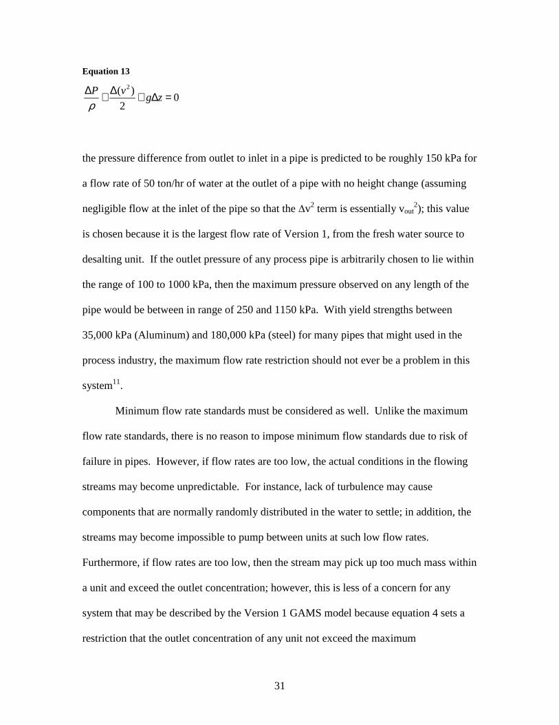
Equation 13

02

)( 2

=∆+∆+∆zg

vP

ρ

the pressure difference from outlet to inlet in a pipe is predicted to be roughly 150 kPa for

a flow rate of 50 ton/hr of water at the outlet of a pipe with no height change (assuming

negligible flow at the inlet of the pipe so that the ∆v2 term is essentially vout2); this value

is chosen because it is the largest flow rate of Version 1, from the fresh water source to

desalting unit. If the outlet pressure of any process pipe is arbitrarily chosen to lie within

the range of 100 to 1000 kPa, then the maximum pressure observed on any length of the

pipe would be between in range of 250 and 1150 kPa. With yield strengths between

35,000 kPa (Aluminum) and 180,000 kPa (steel) for many pipes that might used in the

process industry, the maximum flow rate restriction should not ever be a problem in this

system11.

Minimum flow rate standards must be considered as well. Unlike the maximum

flow rate standards, there is no reason to impose minimum flow standards due to risk of

failure in pipes. However, if flow rates are too low, the actual conditions in the flowing

streams may become unpredictable. For instance, lack of turbulence may cause

components that are normally randomly distributed in the water to settle; in addition, the

streams may become impossible to pump between units at such low flow rates.

Furthermore, if flow rates are too low, then the stream may pick up too much mass within

a unit and exceed the outlet concentration; however, this is less of a concern for any

system that may be described by the Version 1 GAMS model because equation 4 sets a

restriction that the outlet concentration of any unit not exceed the maximum

32

concentration allowed. The actual value of the minimum flow rate standard will be

highly dependent upon the roughness and diameter of the pipe chosen, any elevation

differences between the two ends of the pipe, and the bends and fittings along a pipe’s

length. Thus, any changes made to the Version 1 GAMS model to incorporate a

minimum flow rate in pipes could only be made with arbitrary values to show how such a

process would be carried out once the minimum has been chosen; this is, of course, the

best option in the absence of any information about the piping to be used. To show how

such a change would be made to the model, a minimum flow rate of 0.1 ton/hr is

arbitrarily used.

An effective way to incorporate the minimum flow rate standard into the GAMS

model is to use a binary variable, or binary marker, that is associated with each stream;

thus for all streams between units, or all Fi,i, there are a binary markers associated with

them called Yi,i. The binary marker is used to assure that the flow rate of any stream

between units is within the bounds of the allowable rates. Though it has already been

shown that there is no need to incorporate a maximum flow rate in the GAMS models, an

arbitrarily large maximum flow rate will need to be used in this case so that the bounds

are set for the binary marker equation. This equation is as follows:

Equation 14

maxiiiiminii FYFFY ×≤≤× ,,,

If the flow rate of a stream is below the minimum standard for the system after its value

has initially been calculated (or, likewise, above the maximum), then the binary variable

is forced to be zero, and this action resets the flow rate of the stream to zero; otherwise,

33

the binary variable is set as 1, and the flow rate of the stream is unaltered after the

calculation of its original value. As can be seen from the above equation, if there is no

maximum flow rate used, then the model will always allow the binary variable to be zero;

and so the necessity for the use of an arbitrary, large maximum flow rate becomes

evident. This equation is only incorporated into the non-linear portion of the

optimization; the model that incorporates this binary variable is known as Version 2. The

flow rates of streams between units as predicted by Version 2 with consumption

minimization are shown below in the same manner as before.


Fresh Water Source 79.343 3.E+01 8.571 9.828 0 0 n/a 122.742Caustic Treating 0 0 0 0 80.478 0 0 80.478Distillation 0.1 0 0 0.517 2.847 0 21.536 25Amine Sweetening 1.035 0 0 0 0 0 7.536 8.571Merox I Sweetening 0 0 0 0 0 0 10.345 10.345Hydrotreating 0 0 0 0 0.1 83.325 0 83.425Desalting 0 0 0 0 0 0 83.325 83.325


Destination

Orig

in

Table 6: Flow rates of streams in tons per hour from a unit or fresh water source to another unit or waste water sink as determined by Version 2.

Table 6 shows that the Version 2 model predicts a fresh water requirement of 122.7

ton/hr to the system. However, Table 5 predicts that there exists at least one setup that

will result in a lower fresh water requirement (119.3 ton/hr) than this, while still having

all flow rates above the arbitrary minimum. This is not very surprising, though, because

the particular solver used for the optimization does not allow enough iterations and the

output file states each time that the value is not guaranteed as the absolute optimum; there

exists a way to increase the number of iterations used by altering and referencing an

34

options file (DICOPT.opt), but licensing restrictions prevented this from being done with

the particular version of GAMS used.

4 . VERSION 3

Version 2 provides a universal method to ensure minimum flow rate standards are

met; no matter the number of units in the system, as long as the minimum is set within

the model as a parameter, each stream that exists will not have a flow rate below the

minimum. However, the solver restrictions eliminate the guarantee of global

optimization and the only way to remove such restrictions is by increasing the number of

iterations used; but, an increase in iterations also means that the requirement of a pc to

finish the calculations and find the absolute optimal configuration also increases. Thus,

while Version 2 reduces the resource expenditure of the interface user, it expends many

resources of the pc on which it is run and it will not always guarantee a completely

reliable solution.

To overcome the problems of Version 2 while still ensuring the minimum flow

rate standards are met, a new method of minimization must be used. This new method

greatly resembles Version 1, and so it could be considered another extension of use of

Version 1, or Version “1a”; however, to continue the used numbering system, this will be

referred to as Version 3. In Version 3, the same structure of Version 1 is used, while the

idea behind the binary markers used in Version 2 is called into play as well. In Version

3, the user must manually set each stream flow rate to zero if it falls below the minimum

standard. If, after setting the first stream to zero, any other streams become less than the

minimum or remain less than the minimum (if more than one stream initially falls below

the minimum), then another stream will be chosen to be set to zero; this process continues

35

until all streams are above the minimum flow rate standard. This process was applied as

Version 3 of the GAMS model and it was determined that there are six combinations of

streams that can be set to zero that result in all other streams being greater than the

minimum standard. These combinations are (F1,5, F2,1, F2,4, and F2,5); (F1,5, F2,1, F2,5, F3,5,

F1,1, and F5,1); (F1,5, F2,1, F2,5, F3,5, and F5,1); (F1,5, F2,1, F2,5, F3,5, and F3,1); (F5,1); and

(F3,1). To illustrate the methods of Version 3, F3,1 is arbitrarily chosen to be set to zero.

The flow rates of streams resulting from the minimization of consumption in the Version

3 model are shown below.


Fresh Water Source 2.4 25 8.571 8.388 24.445 50.518 n/a 119.322Caustic Treating 0.267 0 0 1.645 0.775 0 0 2.687Distillation 0 0 0 0.312 0 2.974 21.715 25.001Amine Sweetening 0 0 0 0 0 8.571 0 8.571Merox I Sweetening 0 0 0 0 0 0 10.345 10.345Hydrotreating 0 0 0 0 2.905 25.21 0 28.115Desalting 0 0 0 0 0 0 87.273 87.273


Destination

Orig

in

Table 7: Flow rates of streams in tons per hour from a unit or fresh water source to another unit or waste water sink as determined by Version 3

Comparison of Tables 5 and 7 indicates incredible similarities in the setup of the piping

network predicted by Version 3 and that represented in literature1. As was the case with

the network predicted by Version 1, the only significant difference between the network

predicted by Version 3 and that of published results is the existence of extra streams,

notably two acting as internal recycles from and back to both the caustic treating and

desalting units. Probably the most important conclusion of the piping network predicted

by Version 3 is that, for this particular setup, there is indeed a way to predict a setup that

will result in the same fresh water usage as was predicted in prior studies.

36

5 . VERSION 4

The final version of the GAMS model that was used is called Version 4. In this

version, internal regeneration is incorporated into the model. The reason for this is that,

after treatment, a stream will have its contaminants reduced to a level that make the

stream potentially appropriate for reuse within the system. To make this idea of use, new

equations must be incorporated into the model; one describes the material balances

around each regenerator, another is an overall mass balance, and the last finds the

concentrations of contaminants at the regenerators. In addition, already existing

equations must be updated to include flow from the regenerators to units; this includes

the material balances around units, the linearization equations, and the cost equation.

Unfortunately, there is no good way to describe flow between regenerators in the

GAMS models because, without good initial guesses, each equation that determines flow

between two units will be self-referential. Instead, the three regenerators are combined in

different ways to be modeled as seven new regenerators; the first three of the seven new

regenerators are the same as the three original regenerators, the fourth new regenerator is

a combination of the first and second original ones, the fifth is a combination if the first

and third original regenerators, the sixth is a combination of the second and third original

ones, and the seventh is a combination of all three original regenerators. The outlet

concentrations of treated contaminants of each new, combined regenerator are the

combination of the outlet concentration of the two or three original regenerators that the

new one models.

The first new equation that was added to Version 4 was an overall mass balance.

This was not required in Version 1 because mass balances on each unit could be summed

37

to yield the overall mass balance; in other words, the overall mass balance of the system

was eliminated as a variable due to the connectivity between the six units, the use of a

single fresh water source, and the use of a single waste water sink. However, with

internal regeneration incorporated into the system, this is no longer the case, as the

regenerators receive no fresh water and send nothing to the sink. The equation describing

the overall mass balance is as follows.

Equation 15

∑∑ ∑∑=w u s u

suuw FSFW ,,

The above equation sets the sum of all flow rates of fresh water from a source to all units

for all sources equal to the flow rates of waste water to a sink from all units for all sinks

equal; in other words, it assures that the total flow rate of water entering the system is

equal to the total flow rate of water leaving the system. Equation 14 is incorporated into

both the linear and non-linear portions of the model.

After this, equations were added to describe the concentration of contaminants

coming out of a regenerator. However, this is not as simple of a problem as subtracting a

negative mass load from the concentration of the contaminants going into the regenerator;

instead, the concentration of treated contaminants will leave each regenerator at a set

value, no matter the inlet concentration of the contaminants (within reason).

Furthermore, the untreated contaminants leaving any regenerator will have to have the

same concentration as before entering the regenerator, just after all streams have mixed.

38

Thus, two equations are used to describe the concentration of contaminants leaving the

regenerators. The first of these equations is as follows:

Equation 16

∑ ∑ ×=×u u

outcuruur

mixcr CFRFRC )( ,,,,

Equation 15 sets the mixed concentration of a contaminant equal to the flow rate-

weighted average of the concentrations of each contaminant in each stream going into the

regenerator; the superscript “mix” indicates that it is the concentration of the mixed

streams. Next, the outlet concentration of a contaminant is calculated with the use of

another binary value. This equation is represented below.

Equation 17

*,,,, crcr

mixcr

outcr CXCC +×=

In this equation, there are two user-input parameters: the binary value, Xr,c, and the user

specified outlet concentration from the regenerator, *,crC . If the concentration of a

contaminant is indeed reduced in a regenerator, then *,crC will be the value of the

contaminant’s outlet concentration and Xr,c will have a value of zero. On the other hand,

if a regenerator does not treat a contaminant, then *,crC will have a value of zero and Xr,c

will have a value of one. Thus, the outlet concentration of a contaminant from a

39

regenerator is set to be either the user-specified outlet concentration, or the mixed

concentration; equations 15 and 16 are only used in the non-linear portion of the model.

The equation that is added to Version 1 as part of Version 4 that describes the

mass balance around each regenerator is described below.

Equation 18

∑∑ =u

ur

u

ru FRFR ,,

This equation states that the sum of flow rates of all streams going into a regenerator

must be equal to the sum of all flow rates of streams leaving a regenerator; because of the

way the three regenerators are combined to make seven new regenerators, the flow both

into and leaving regenerators is strictly between units. Equation 17 is incorporated into

both the linear and non-linear parts of the model.

The mass balance around each unit must also be updated to include flow from

regenerators. The new equation describing the mass balance around units is as follows:

Equation 19

∑∑∑∑∑∑ ++=++r

ru

s

su

u

uu

r

ur

u

uu

w

uw FRFSFFRFFWj

ji

j

ij ,,,,,,

The mass balance around units is used as before, but with new terms to describe flow

leaving units to go to regenerators and coming into units from regenerators; “FR”

designates the flow rate of a stream between a unit and a regenerator and the subscript “r”

indicates a regenerator. The equations describing the concentration of contaminants

40

going into and leaving the units were altered to include the regenerators as well. These

two new equations are described by equations 19 and 20.

Equation 20

max,,,,

,,,,,,

)(

)()()(

inu

r

ru

s

su

u

uu

r

outcrurcu

u

uucw

w

uw

ii

j

ji

j

j

ij

CFRFSF

CFRCFCFW

×++

≤×+×+×

∑∑∑

∑∑∑

Equation 21

outu

r

ru

s

sui

u

uu

cu

r

outcrcu

u

uucw

w

uw

i

j

ji

j

j

ij

CFRFSF

MLCuFRrCFCFW

×++

=+×+×+×

∑∑∑

∑∑∑

)(

),()()(

,,,

,,,,,,

The cost function is also updated to include the cost of using the regenerators. This new

cost function is described by:

Equation 22

008760.0)))(())(())((( ,,, ××+×+×= ∑ ∑ ∑ ∑ ∑∑w u s r

rru

u

ssu

u

wuw PFRPFWPFWCost

The price of using the regenerators is determined by multiplying the flow rate of water

through the regenerator by the cost of operation; the cost of regenerators 4 through 7 is

the combined cost of the individual regenerators that they model (i.e. the cost of using

regenerator 4 is the same as the combined cost of using regenerators 1 and 2). Finally,

the linearization equations are updated to include the regenerators. They are as follows:

41

Equation 23

maxincu

r

ru

s

su

u

uu

crcrmaxout

cur

urmaxout

cuju

uucw

w

uw

ii

j

ji

j

ij

CFRFSF

CXCFRCFCFW

,,,,,

*,,

,,,

,,,,,

)(

))(()()(

×++

≤+××+×+×

∑∑∑

∑∑∑

Equation 24

outcu

r

ru

s

su

u

uu

cu

rcrcr

maxoutcuur

maxoutcuj

u

uucw

w

uw

ii

j

ji

j

ij

CFRFSF

MLCXCFRCFCFW

,,,,

,*,,

,,,

,,,,,

)(

))(()()(

×++=

++××+×+×

∑∑∑

∑∑∑

And, the equation setting the outlet concentration of the units to its maximum value is

eliminated in Version 4 because it becomes redundant. The network of streams and their

flow rates that are predicted by Version 4 when using a consumption minimization are

tabulated below.

Caust. Dist. Am.Sw. M1S Hydr. Desalt API/ACA RO CWWT Sink Sum from Source

Fresh Water Source 0 25 8.571 0 0 0 n/a n/a n/a n/a 33.571Caustic Treating 0 0 0 0.014 0 0 2.55 0 0 0.1 2.664Distillation 0 0 0 0 0.016 0.013 19.814 0 0 5.156 24.999Amine Sweetening 0 0 0 0 0 0 8.471 0 0 0.1 8.571Merox I Sweetening 0 0 0 0 0 0 0 0 0 10.085 10.085Hydrotreating 0 0 0 0 0 0 29.893 0 0 0.1 29.993Desalting 0 0 0 0 0 0 56.396 0 0 18.03 74.426API and ACA 0 0 0 0 0 0 n/a 88.838 28.289 n/a 117.127Reverse Osmosis 1.333 0 0 2.187 10.905 74.413 n/a n/a 0 n/a 88.838Chevron WWT 1.333 0 0 7.885 19.072 0 0 n/a n/a n/a 28.29

Sum to Destination 2.666 25 8.571 10.086 29.993 74.426 117.124 88.838 28.289 33.571

Destination

Orig

in

Table 8: Flow rates of streams in tons per hour from a unit, regenerator, or fresh water source to another unit or regenerator, or the waste water sink as described by Version 4.

Initial inspection of Table 8 first shows that the minimum flow rate standard is not being

accounted for in the Version 4 model; however, the methods used in Version 3 could

42

easily be applied to Version 4 so that the minimum flow standards are met. For the sake

of exploring how well the GAMS model predicts the piping network with regeneration,

though, it is unnecessary to incorporate a minimum flow rate standard, as this was a

separate investigation. In addition, Table 8 indicates that Version 4 predicts a fresh water

requirement of 33.57 ton/hr; this is the same value predicted in literature, and so the

accuracy of the Version 4 model is affirmed1.

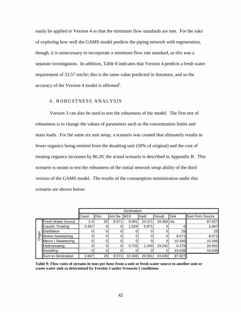
6 . ROBUSTNESS ANALYSIS

Version 3 can also be used to test the robustness of the model. The first test of

robustness is to change the values of parameters such as the concentration limits and

mass loads. For the same six unit setup, a scenario was created that ultimately results in

fewer organics being emitted from the desalting unit (50% of original) and the cost of

treating organics increases by $0.20; the actual scenario is described in Appendix B. This

scenario is meant to test the robustness of the initial network setup ability of the third

version of the GAMS model. The results of the consumption minimization under this

scenario are shown below:

Table 9: Flow rates of streams in tons per hour from a unit or fresh water source to another unit or waste water sink as determined by Version 3 under Scenario 1 conditions


Fresh Water Source 2.4 25 8.571 8.091 24.371 19.394 n/a 87.827Caustic Treating 0.267 0 0 1.529 0.871 0 0 2.667Distillation 0 0 0 0 0 0 25 25Amine Sweetening 0 0 0 0 0 0 8.571 8.571Merox I Sweetening 0 0 0 0 0 0 10.345 10.345Hydrotreating 0 0 0 0.725 1.349 24.242 0.275 26.591Desalting 0 0 0 0 0 0 43.636 43.636


Destination

Orig

in

43

No prior study has been carried out with the altered values of parameters pertaining to

organics, though the fresh water requirement is on the same order as each of the prior

results in Tables 4 through 8, so the results seem reasonable. Unfortunately, the study of

Version 3’s applicability in Scenario 1 only provides a trivial idea as to the robustness of

the GAMS models; it is of little use in an industrial application to be able to predict what

the new piping network will be when parameters change, because the costs of redoing the

network would likely be incredibly steep. Indeed, the results in Table 9 merely indicate

that Version 3 will not lead to catastrophic failure when the values of parameters are

changed. Table 9 verifies that Version 3 can predict the setup of a piping network and

flow rates to and from units within that network that will result in the minimum water

consumption, and a true test of robustness of the GAMS models is to fix the setup of that

network and test what the new flow rates to and from units within the network will be

when parameter values change. Thus, another robustness study is carried out to test this

situation; however, to make the robustness check more general, the model used for this

check was Version 2. To do this, the linear and non-linear outlet concentration equations,

equations 3 and 9, were split into two equations and each optimized model was split into

two models, the first with the first outlet concentration equations and the second model

with the second outlet concentration equations. In addition, a second set of mass loads

was defined as parameters for the second outlet concentration equations; for this scenario,

the value of each mass load in the second set is double the corresponding mass loads in

the second set. After the initial minimization was carried out, the values of the binary

markers, Yi,i, were fixed at their current level for the remainder of the optimization.

Inspection of equation 13 shows that the binary marker forces streams to exist if and only

44

if their flow rate is greater than or equal to the minimum standard, thus their value also

determines whether or not a stream between units exists; therefore, fixing values of the

binary markers also fixes the setup of the piping network. After the setup has been fixed,

a new minimization is carried out with second set of mass loads via the second set of

outlet concentration equations. This set of conditions is referred to as Scenario 2.

Under the Scenario 2 conditions, the expectation is that the fresh water

requirements will double because the mass loads of each unit have doubled; if the fresh

water requirements do not double under Scenario 2, then the Version 2 model of GAMS,

and potentially each of the other 3 GAMS models, will only be useful for providing the

initial setup of a piping network based on initial values of concentration limits and mass

loads of units. Using the modified Version 2 model to minimize the consumption first

under normal conditions, then in Scenario 2, the following results were obtained:

Table 10: Flow rates of streams in tons per hour from a unit or fresh water source to another unit or waste water sink determined by the modified Version 2 not under Scenario 2 conditions


Fresh Water Source 33.417 25 8.571 9.828 45.541 0 n/a 122.357Caustic Treating 0 0 0 0 33.901 0 0 33.901Distillation 0 0 0 0.517 0.2 0 24.283 25Amine Sweetening 0.484 0 0 0 3.674 0 4.413 8.571Merox I Sweetening 0 0 0 0 0 0 10.345 10.345Hydrotreating 0 0 0 0 0.2 83.316 0 83.516Desalting 0 0 0 0 0 0 83.316 83.316


Destination

Orig

in

45

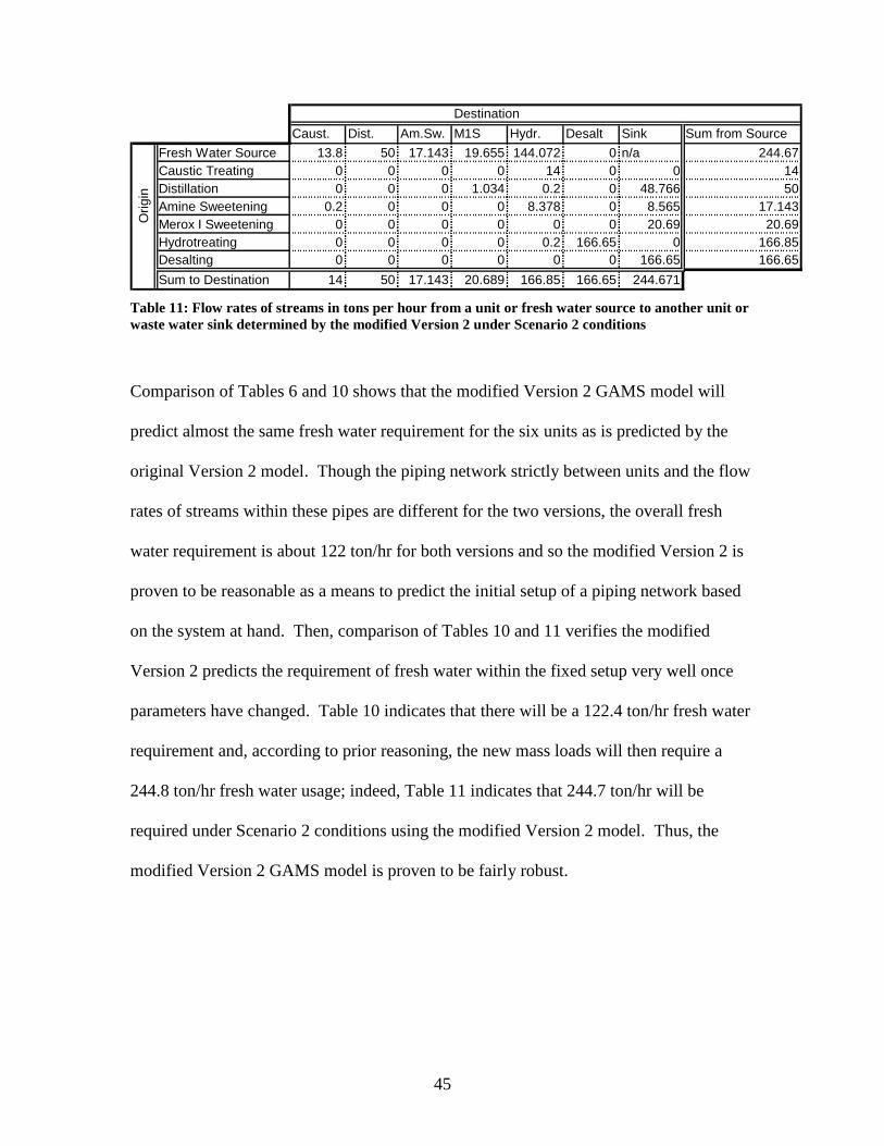
Table 11: Flow rates of streams in tons per hour from a unit or fresh water source to another unit or waste water sink determined by the modified Version 2 under Scenario 2 conditions

Comparison of Tables 6 and 10 shows that the modified Version 2 GAMS model will

predict almost the same fresh water requirement for the six units as is predicted by the

original Version 2 model. Though the piping network strictly between units and the flow

rates of streams within these pipes are different for the two versions, the overall fresh

water requirement is about 122 ton/hr for both versions and so the modified Version 2 is

proven to be reasonable as a means to predict the initial setup of a piping network based

on the system at hand. Then, comparison of Tables 10 and 11 verifies the modified

Version 2 predicts the requirement of fresh water within the fixed setup very well once

parameters have changed. Table 10 indicates that there will be a 122.4 ton/hr fresh water

requirement and, according to prior reasoning, the new mass loads will then require a

244.8 ton/hr fresh water usage; indeed, Table 11 indicates that 244.7 ton/hr will be

required under Scenario 2 conditions using the modified Version 2 model. Thus, the

modified Version 2 GAMS model is proven to be fairly robust.


Fresh Water Source 13.8 50 17.143 19.655 144.072 0 n/a 244.67Caustic Treating 0 0 0 0 14 0 0 14Distillation 0 0 0 1.034 0.2 0 48.766 50Amine Sweetening 0.2 0 0 0 8.378 0 8.565 17.143Merox I Sweetening 0 0 0 0 0 0 20.69 20.69Hydrotreating 0 0 0 0 0.2 166.65 0 166.85Desalting 0 0 0 0 0 0 166.65 166.65

Sum to Destination 14 50 17.143 20.689 166.85 166.65 244.671

Destination

Orig

in

46

V . C O N C L U S I O N S

Studies of the applicability of several GAMS models have been carried out. Each

of the models is designed to minimize fresh water consumption in a system of six water-

using units with four contaminants; each is also based on a template model, Version 0.

The first model, Version 1, studies the general applicability of the series of models by

placing no restrictions on flow rates. Results from this study indicate the same fresh

water requirement as predicted in literature1; thus, the general use of the models is

affirmed as reasonable. The second model, Version 2, imposes the restriction of

minimum flow rates in the piping networks predicted by the model; this version does this

by use of binary markers that have the ability to “turn on” or “turn off” the existence of

streams in the network. The results from this study predict a fresh water requirement

reasonably close as was predicted by Version 1. However, the requirement is slightly

higher and no global optimum is guaranteed by Version 2. The third model, Version 3,

continues to impose the restriction of minimum flow rates, this time calling for the user to

manually “turn off” streams. This model predicts the same fresh water consumption

predicted by Version 1. The final version of all models, Version 4, incorporates

regeneration into Version 1. The fresh water requirement decreases to about one third of

the values predicted by the three prior versions. In addition, the results of Version 4

agree well with those in literature1. In all, the four versions verify that an interface such

as GAMS is appropriate to create or modify algorithms to minimize fresh water

consumption in process industries.

47

V I . F U T U R E W O R K A N D R E C O M M E N D A T I O N S

Comparison of the networks predicted in Tables 4, 5, and 7 shows that several

different combinations of streams can be utilized to result in the same fresh water

consumption. However, these results do not take into account the actual cost of

purchasing and installing the networks; if this consideration is applied, Table 5 will likely

lead to the most cost effective network of the three. This brings to light the necessity of

including piping cost into the cost equation (eqs. 7, 12, and 22) of the algorithms. Thus,

the most immediate recommendation is to include piping costs into the total cost.

Other areas of consideration are:

1. Including the costs associated with including the additional treatment units into

the model,

2. Comparison of other available treatment processes,

3. Removal of other contaminants from process water,

4. Improvement upon the assumptions associated with outlet concentrations from

treatment units, and

5. Use of other modeling interfaces for the system optimization.

48

R E F E R E N C E S 1. Koppol, A.P., et al. Adv. in Env. Res., V(8), 2003, 151-171. 2. Perlman, Howard A. Uses of water. 2007. http://www.waterencyclopedia.com/Tw-

Z/Uses-of-Water.html. 3. Profile of the Petroleum Refining Industry. Environmental Protection Agency.

September 1995. http://www.cluin.org/download/toolkit/petrefsn.pdf 4. Petroleum Refining Corrosion. The Hendrix Group, Inc. April 2007.

http://www.hghouston.com/refining.html#crudedist 5. Cartwright, Peter. Process Water Treatment – Challenges and Solutions. Chemical

Engineering Magazine. March 2006. 6. Type of API separators. Triveni Engineering & Industries Ltd.

http://www.trivenigroup.com/water/api-separator.html 7. API separator. Monroe Environmental Corporation. 2005.

http://www.monroeenvironmental.com/clarifier-api-separator.htm 8. API separators – Application Data Sheet. Emerson process management. August

2006. http://www.emersonprocess.com/raihome/documents/Liq_AppData_2900-08.pdf

9. Fisher, Arthur et-al. Reverse Osmosis – How it works. University of Nevada.

http://ag.arizona.edu/region9wq/pdf/nv_ROhow.pdf. 10. Chevron waste water treatment – Process. Chevron Products Company, San

Ramon, CA. 2007. http://www.chevron.com/products/prodserv/refiningtechnology/waste_wtr_treat_6b.shtm

11. Callister, William D. Jr. Materials Science and Engineering: An Introduction,6 Ed.

J. Wiley & Sons: New York, NY. 2002. pg. 129

49

A P P E N D I C E S APPENDIX A : GAMS MODELS

The following are the important versions used in the GAMS interface for optimizations.

In some cases, comments have been removed to make the whole of the program less

confusing. Any of these versions should be able to pasted directly into GAMS and run

with the same results presented in the body of this work.

Version 0 Set u water using units / 1*3 / w freshwater source / 1 / s wastewater sink / 1 / c Contaminant / 1*3 /; Alias(u,ua); Parameters CFW(w) Cost of freshwater / 1 0.3 / CWW(s) Cost of wastewater treatment / 1 0.75 /; Table ConFW(w,c) Freshwater source concentration 1 2 3 1 0 0 0; Table Cinmax(u,c) maximum inlet concentration in the units 1 2 3 1 0 0 0 2 20 300 45 3 120 20 200; Table Coutmax(u,c) maximum outlet concentration in the units 1 2 3 1 15 400 35 2 120 12500 180 3 220 45 9500; Table ConWW(s,c) Concentration limits at the sink

50

1 2 3 1 10000000 10000000 100000000; Table ML(u,c) Mass Load 1 2 3 1 675 18000 1575 2 3400 414800 4590 3 5600 1400 520800; Variable FW(w,u) Flowrates between freshwater sources and units F(u,u) Flowrates between units FS(u,s) Flowrates between units and sinks Cout(u,c) Outlet concentration in the units Cost Cost Consu Consumption; Positive variable FW,F,FS,Cout; Equations waterbalance(u) Balance of water inlet(u,c) Limit of inlet concentration of the units outlet(u,c) Calculation of outlet concentration of the units maxout(u,c) Limit of outlet concentration of the units sink(s,c) Limit of inlet concentration of the sinks ObjCost Objective function that minimizes cost ObjConsu Objective function that minimizes cosumption **Linear - Starting points inletl(u,c) Limit of inlet concentration of the units outletl(u,c) Calculation of outlet concentration of the units maxoutl(u,c) Limit of outlet concentration of the units ; waterbalance(u) ..sum(w,FW(w,u))+sum(ua,F(ua,u))=e=sum(ua,F(u,ua))+sum(s,FS(u,s)); inlet(u,c) ..sum(w,FW(w,u)*ConFW(w,c))+sum(ua,F(ua,u)*Cout(ua,c))=L=(sum(ua,F(u,ua))+sum(s,FS(u,s)))*Cinmax(u,c); outlet(u,c) ..sum(w,FW(w,u)*ConFW(w,c))+sum(ua,F(ua,u)*Cout(ua,c))+ML(u,c)=E=(sum(ua,F(u,ua))+sum(s,FS(u,s)))*Cout(u,c); maxout(u,c) ..Cout(u,c)=L=Coutmax(u,c); sink(s,c) ..sum(u,FS(u,s)*(Cout(u,c)-ConWW(s,c)))=L=0; ObjCost ..Cost=e=sum(w,sum(u,FW(w,u))*cfw(w))+sum(s,sum(u,FS(u,s))*cww(s)); ObjConsu ..Consu=e=sum(w,sum(u,FW(w,u)));

51

**Linear - Starting points inletl(u,c) ..sum(w,FW(w,u)*ConFW(w,c))+sum(ua,F(ua,u)*Coutmax(ua,c))=L=(sum(ua,F(u,ua))+sum(s,FS(u,s)))*Cinmax(u,c); outletl(u,c) ..sum(w,FW(w,u)*ConFW(w,c))+sum(ua,F(ua,u)*Coutmax(ua,c))+ML(u,c)=E=(sum(ua,F(u,ua))+sum(s,FS(u,s)))*Coutmax(u,c); maxoutl(u,c) ..Cout(u,c)=e=Coutmax(u,c); MODEL Reuse / waterbalance,inlet,outlet,maxout,sink,ObjCost,ObjConsu /; MODEL Start / waterbalance,inletl,outletl,maxoutl,ObjCost,ObjConsu /; *SOLVE Start using LP minimizing cost; SOLVE Start using LP minimizing consu; *SOLVE Reuse using NLP minimizing cost; SOLVE Reuse using NLP minimizing consu; DISPLAY Cost.l,Consu.l,FW.l,F.l,FS.l,Cout.l; Version 1 (cf. Table 1) Set u water using units / 1*6 / w freshwater source / 1 / s wastewater sink / 1 / c Contaminant / 1*4 /; Alias(u,ua); Parameters CFW(w) Cost of freshwater in $ per ton / 1 .32 / CWW(s) Cost of wastewater treatment $ per ton / 1 1.68 /; Table ConFW(w,c) Freshwater source concentration in ppm 1 2 3 4 1 0 0 0 0; Table Cinmax(u,c) maximum inlet concentration in the units in ppm 1 2 3 4 1 300 50 5000 1500 2 10 1 0 0 3 10 1 0 0 4 100 200 50 1000

52

5 85 200 300 200 6 1000 1000 150 200; Table Coutmax(u,c) maximum outlet concentration in the units in ppm 1 2 3 4 1 500 500 11000 3000 2 200 4000 500 1000 3 1000 3500 2000 3500 4 400 6000 2000 3500 5 350 1800 6500 1000 6 9500 6500 450 400; Table ConWW(s,c) Concentration limits at the sink in ppm 1 2 3 4 1 10000000000 10000000000 10000000000 10000000000; Table ML(u,c) Mass Load (transfered to water at unit) in g per hour 1 2 3 4 1 180 1200 750 100 2 3610 100000 250 800 3 600 30000 1500 1000 4 2000 60000 800 1000 5 3800 45000 1100 2000 6 120000 480000 1500 0; Variable FW(w,u) Flowrates between freshwater sources and units in ton per hour F(u,u) Flowrates between units in ton per hour FS(u,s) Flowrates between units and sinks in ton per hour Cout(u,c) Outlet concentration in the units in ppm Cost Cost in $Mil per year Consu Consumption in ton per hour; Positive variable FW,F,FS,Cout; Equations waterbalance(u) Balance of water inlet(u,c) Limit of inlet concentration of the units outlet(u,c) Calculation of outlet concentration of the units maxout(u,c) Limit of outlet concentration of the units sink(s,c) Limit of inlet concentration of the sinks ObjCost Objective function that minimizes cost ObjConsu Objective function that minimizes cosumption **Linear - Starting points inletl(u,c) Limit of inlet concentration of the units

53

outletl(u,c) Calculation of outlet concentration of the units maxoutl(u,c) Limit of outlet concentration of the units; waterbalance(u) ..sum(w,FW(w,u))+sum(ua,F(ua,u))=e=sum(ua,F(u,ua))+sum(s,FS(u,s)); inlet(u,c) ..sum(w,FW(w,u)*ConFW(w,c))+sum(ua,F(ua,u)*Cout(ua,c))=L=(sum(ua,F(u,ua))+sum(s,FS(u,s)))*Cinmax(u,c); outlet(u,c) ..sum(w,FW(w,u)*ConFW(w,c))+sum(ua,F(ua,u)*Cout(ua,c))+ML(u,c)=E=(sum(ua,F(u,ua))+sum(s,FS(u,s)))*Cout(u,c); maxout(u,c) ..Cout(u,c)=L=Coutmax(u,c); sink(s,c) ..sum(u,FS(u,s)*(Cout(u,c)-ConWW(s,c)))=L=0; ObjCost ..Cost=e=(sum(w,sum(u,FW(w,u))*cfw(w))+sum(s,sum(u,FS(u,s))*cww(s)))*0.008760; **This cost assumes constant operation **The "*0.008760" term comes from 8760 hours opperated per year and divided by 1E6 to get units of millions of dollars ObjConsu ..Consu=e=sum(w,sum(u,FW(w,u))); **Linear - Starting points inletl(u,c) ..sum(w,FW(w,u)*ConFW(w,c))+sum(ua,F(ua,u)*Coutmax(ua,c))=L=(sum(ua,F(u,ua))+sum(s,FS(u,s)))*Cinmax(u,c); outletl(u,c) ..sum(w,FW(w,u)*ConFW(w,c))+sum(ua,F(ua,u)*Coutmax(ua,c))+ML(u,c)=E=(sum(ua,F(u,ua))+sum(s,FS(u,s)))*Coutmax(u,c); maxoutl(u,c) ..Cout(u,c)=e=Coutmax(u,c); MODEL Reuse / waterbalance,inlet,outlet,maxout,sink,ObjCost,ObjConsu/; MODEL Start / waterbalance,inletl,outletl,maxoutl,ObjCost,ObjConsu/; *SOLVE Start using rMIP minimizing Cost; *SOLVE Start using MIP minimizing Cost; SOLVE Start using MIP minimizing consu; SOLVE Reuse using MINLP minimizing Cost; *SOLVE Reuse using MINLP minimizing consu; DISPLAY Cost.l,Consu.l,FW.l,F.l,FS.l,Cout.l; Version 2 (cf. Table 3) Set u water using units / 1*6 / w freshwater source / 1 / s wastewater sink / 1 / c Contaminant / 1*4 /;

54

Alias(u,ua); Parameters CFW(w) Cost of freshwater / 1 .32 / CWW(s) Cost of wastewater treatment / 1 1.68 /; Table ConFW(w,c) Freshwater source concentration 1 2 3 4 1 0 0 0 0; Table Cinmax(u,c) maximum inlet concentration in the units 1 2 3 4 1 300 50 5000 1500 2 10 1 0 0 3 10 1 0 0 4 100 200 50 1000 5 85 200 300 200 6 1000 1000 150 200; Table Coutmax(u,c) maximum outlet concentration in the units 1 2 3 4 1 500 500 11000 3000 2 200 4000 500 1000 3 1000 3500 2000 3500 4 400 6000 2000 3500 5 350 1800 6500 1000 6 9500 6500 450 400; Table ConWW(s,c) Concentration limits at the sink 1 2 3 4 1 100000000 100000000 100000000 100000000; Table ML(u,c) Mass Load g per hr 1 2 3 4 1 180 1200 750 100 2 3610 100000 250 800 3 600 30000 1500 1000 4 2000 60000 800 1000 5 3800 45000 1100 2000 6 120000 480000 1500 0; Parameter Minflow Minimum flowrate allowed / .2 /; Parameter Maxflow Maximum flowrate allowed / 10000 /;

55

Variable FW(w,u) Flowrates between freshwater sources and units F(ua,u) Flowrates between units FS(u,s) Flowrates between units and sinks Cout(u,c) Outlet concentration in the units Cost Cost Consu Consumption Y(ua,u) The binary Y switch; Positive variable FW,F,FS,Cout; Binary variable Y; Equations waterbalance(u) Balance of water inlet(u,c) Limit of inlet concentration of the units outlet(u,c) Calculation of outlet concentration of the units maxout(u,c) Limit of outlet concentration of the units sink(s,c) Limit of inlet concentration of the sinks ObjCost Objective function that minimizes cost ObjConsu Objective function that minimizes cosumption **Linear - Starting points inletl(u,c) Limit of inlet concentration of the units outletl(u,c) Calculation of outlet concentration of the units maxoutl(u,c) Limit of outlet concentration of the units YcheckL(ua,u) Check to be sure that the flowrates are above the minimum YcheckH(ua,u) Check to be sure that the flowrates are below the maximum; waterbalance(u) ..sum(w,FW(w,u))+sum(ua,F(ua,u))=e=sum(ua,F(u,ua))+sum(s,FS(u,s)); inlet(u,c) ..sum(w,FW(w,u)*ConFW(w,c))+sum(ua,F(ua,u)*Cout(ua,c))=L=(sum(ua,F(u,ua))+sum(s,FS(u,s)))*Cinmax(u,c); outlet(u,c) ..sum(w,FW(w,u)*ConFW(w,c))+sum(ua,F(ua,u)*Cout(ua,c))+ML(u,c)=E=(sum(ua,F(u,ua))+sum(s,FS(u,s)))*Cout(u,c); maxout(u,c) ..Cout(u,c)=L=Coutmax(u,c); sink(s,c) ..sum(u,FS(u,s)*(Cout(u,c)-ConWW(s,c)))=L=0; ObjCost ..Cost=e=(sum(w,sum(u,FW(w,u))*cfw(w))+sum(s,sum(u,FS(u,s))*cww(s)))*.008760; ObjConsu ..Consu=e=sum(w,sum(u,FW(w,u))); **Linear - Starting points

56

inletl(u,c) ..sum(w,FW(w,u)*ConFW(w,c))+sum(ua,F(ua,u)*Coutmax(ua,c))=L=(sum(ua,F(u,ua))+sum(s,FS(u,s)))*Cinmax(u,c); outletl(u,c) ..sum(w,FW(w,u)*ConFW(w,c))+sum(ua,F(ua,u)*Coutmax(ua,c))+ML(u,c)=E=(sum(ua,F(u,ua))+sum(s,FS(u,s)))*Coutmax(u,c); maxoutl(u,c) ..Cout(u,c)=e=Coutmax(u,c); YcheckL(ua,u) ..Y(ua,u)*Minflow=L=F(ua,u); YcheckH(ua,u) ..Y(ua,u)*Maxflow=G=F(ua,u); MODEL Reuse / waterbalance,inlet,outlet,maxout,sink,ObjCost,ObjConsu,YcheckL,YcheckH /; MODEL Start / waterbalance,inletl,outletl,maxoutl,ObjCost,ObjConsu,YcheckL,YcheckH /; *SOLVE Start using rMIP minimizing cost; SOLVE Start using rMIP minimizing consu; *SOLVE Start using MIP minimizing cost; SOLVE Start using MIP minimizing consu; *SOLVE Reuse using MINLP minimizing cost; SOLVE Reuse using MINLP minimizing consu; DISPLAY Cost.l,Consu.l,FW.l,F.l,FS.l,Cout.l,Y.l; Modified Version 2 NOT under Scenario 2 (cf. Table 7) Set u water using units / 1*6 / w freshwater source / 1 / s wastewater sink / 1 / c Contaminant / 1*4 /; Alias(u,ua); Parameters CFW(w) Cost of freshwater / 1 .32 / CWW(s) Cost of wastewater treatment / 1 1.68 /; Table ConFW(w,c) Freshwater source concentration 1 2 3 4 1 0 0 0 0; Table Cinmax(u,c) maximum inlet concentration in the units

57

1 2 3 4 1 300 50 5000 1500 2 10 1 0 0 3 10 1 0 0 4 100 200 50 1000 5 85 200 300 200 6 1000 1000 150 200; Table Coutmax(u,c) maximum outlet concentration in the units 1 2 3 4 1 500 500 11000 3000 2 200 4000 500 1000 3 1000 3500 2000 3500 4 400 6000 2000 3500 5 350 1800 6500 1000 6 9500 6500 450 400; Table ConWW(s,c) Concentration limits at the sink 1 2 3 4 1 100000000 100000000 100000000 100000000; Table ML1(u,c) Initial Mass Load g per hr 1 2 3 4 1 180 1200 750 100 2 3610 100000 250 800 3 600 30000 1500 1000 4 2000 60000 800 1000 5 3800 45000 1100 2000 6 120000 480000 1500 0; $ontext Table ML2(u,c) Final Mass Load g per hr 1 2 3 4 1 360 2400 1500 200 2 7220 200000 500 1600 3 1200 60000 3000 2000 4 4000 120000 1600 2000 5 7600 90000 2200 4000 6 240000 960000 3000 0; $offtext Parameter Minflow Minimum flowrate allowed / 0.1 /; Parameter Maxflow Maximum flowrate allowed / 10000 /; Variable

58

FW(w,u) Flowrates between freshwater sources and units F(ua,u) Flowrates between units FS(u,s) Flowrates between units and sinks Cout(u,c) Outlet concentration in the units Cost Cost Consu Consumption Y(ua,u) The binary Y switch; Positive variable FW,F,FS,Cout; Binary variable Y; Equations waterbalance(u) Balance of water inlet(u,c) Limit of inlet concentration of the units outlet1(u,c) Initial Calculation of outlet concentration of the units * outlet2(u,c) Final Calculation of outlet concentration of the units maxout(u,c) Limit of outlet concentration of the units sink(s,c) Limit of inlet concentration of the sinks ObjCost Objective function that minimizes cost ObjConsu Objective function that minimizes cosumption **Linear - Starting points inletl(u,c) Limit of inlet concentration of the units outletl1(u,c) Initial Calculation of outlet concentration of the units * outletl2(u,c) Final Calculation of outlet concentration of the units maxoutl(u,c) Limit of outlet concentration of the units YcheckL(ua,u) Check to be sure that the flowrates are above the minimum YcheckH(ua,u) Check to be sure that the flowrates are below the maximum; waterbalance(u) ..sum(w,FW(w,u))+sum(ua,F(ua,u))=e=sum(ua,F(u,ua))+sum(s,FS(u,s)); inlet(u,c) ..sum(w,FW(w,u)*ConFW(w,c))+sum(ua,F(ua,u)*Cout(ua,c))=L=(sum(ua,F(u,ua))+sum(s,FS(u,s)))*Cinmax(u,c); outlet1(u,c) ..sum(w,FW(w,u)*ConFW(w,c))+sum(ua,F(ua,u)*Cout(ua,c))+ML1(u,c)=E=(sum(ua,F(u,ua))+sum(s,FS(u,s)))*Cout(u,c); * outlet2(u,c) ..sum(w,FW(w,u)*ConFW(w,c))+sum(ua,F(ua,u)*Cout(ua,c))+ML2(u,c)=E=(sum(ua,F(u,ua))+sum(s,FS(u,s)))*Cout(u,c); maxout(u,c) ..Cout(u,c)=L=Coutmax(u,c); sink(s,c) ..sum(u,FS(u,s)*(Cout(u,c)-ConWW(s,c)))=L=0; ObjCost ..Cost=e=(sum(w,sum(u,FW(w,u))*cfw(w))+sum(s,sum(u,FS(u,s))*cww(s)))*.008760; ObjConsu ..Consu=e=sum(w,sum(u,FW(w,u)));

59

**Linear - Starting points inletl(u,c) ..sum(w,FW(w,u)*ConFW(w,c))+sum(ua,F(ua,u)*Coutmax(ua,c))=L=(sum(ua,F(u,ua))+sum(s,FS(u,s)))*Cinmax(u,c); outletl1(u,c) ..sum(w,FW(w,u)*ConFW(w,c))+sum(ua,F(ua,u)*Coutmax(ua,c))+ML1(u,c)=E=(sum(ua,F(u,ua))+sum(s,FS(u,s)))*Coutmax(u,c); * outletl2(u,c) ..sum(w,FW(w,u)*ConFW(w,c))+sum(ua,F(ua,u)*Coutmax(ua,c))+ML2(u,c)=E=(sum(ua,F(u,ua))+sum(s,FS(u,s)))*Coutmax(u,c); maxoutl(u,c) ..Cout(u,c)=e=Coutmax(u,c); YcheckL(ua,u) ..Y(ua,u)*Minflow=L=F(ua,u); YcheckH(ua,u) ..Y(ua,u)*Maxflow=G=F(ua,u); MODEL Start1 / waterbalance,inletl,outletl1,maxoutl,ObjCost,ObjConsu,YcheckL,YcheckH /; *MODEL Start2 / waterbalance,inletl,outletl2,maxoutl,ObjCost,ObjConsu,YcheckL,YcheckH /; MODEL Reuse1 / waterbalance,inlet,outlet1,maxout,sink,ObjCost,ObjConsu,YcheckL,YcheckH /; *MODEL Reuse2 / waterbalance,inlet,outlet2,maxout,sink,ObjCost,ObjConsu,YcheckL,YcheckH /; *SOLVE Start using rMIP minimizing cost; SOLVE Start1 using rMIP minimizing consu; *SOLVE Start using MIP minimizing cost; SOLVE Start1 using MIP minimizing consu; *Reuse.optfile=1; *SOLVE Reuse using MINLP minimizing cost; SOLVE Reuse1 using MINLP minimizing consu; *Y.fx(ua,u)=Y.l(ua,u); *SOLVE Start2 using rMIP minimizing consu; *SOLVE Start2 using MIP minimizing consu; *SOLVE Reuse2 using MINLP minimizing consu; DISPLAY Cost.l,Consu.l,FW.l,F.l,FS.l,Cout.l,Y.l; Modified Version 2 under Scenario 2 (cf. Table 8) Set u water using units / 1*6 / w freshwater source / 1 / s wastewater sink / 1 / c Contaminant / 1*4 /; Alias(u,ua);

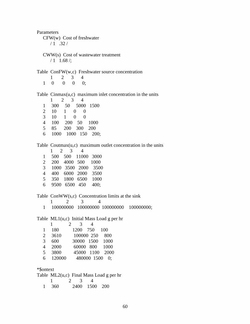
60

Parameters CFW(w) Cost of freshwater / 1 .32 / CWW(s) Cost of wastewater treatment / 1 1.68 /; Table ConFW(w,c) Freshwater source concentration 1 2 3 4 1 0 0 0 0; Table Cinmax(u,c) maximum inlet concentration in the units 1 2 3 4 1 300 50 5000 1500 2 10 1 0 0 3 10 1 0 0 4 100 200 50 1000 5 85 200 300 200 6 1000 1000 150 200; Table Coutmax(u,c) maximum outlet concentration in the units 1 2 3 4 1 500 500 11000 3000 2 200 4000 500 1000 3 1000 3500 2000 3500 4 400 6000 2000 3500 5 350 1800 6500 1000 6 9500 6500 450 400; Table ConWW(s,c) Concentration limits at the sink 1 2 3 4 1 100000000 100000000 100000000 100000000; Table ML1(u,c) Initial Mass Load g per hr 1 2 3 4 1 180 1200 750 100 2 3610 100000 250 800 3 600 30000 1500 1000 4 2000 60000 800 1000 5 3800 45000 1100 2000 6 120000 480000 1500 0; *$ontext Table ML2(u,c) Final Mass Load g per hr 1 2 3 4 1 360 2400 1500 200

61

2 7220 200000 500 1600 3 1200 60000 3000 2000 4 4000 120000 1600 2000 5 7600 90000 2200 4000 6 240000 960000 3000 0; *$offtext Parameter Minflow Minimum flowrate allowed / 0.1 /; Parameter Maxflow Maximum flowrate allowed / 10000 /; Variable FW(w,u) Flowrates between freshwater sources and units F(ua,u) Flowrates between units FS(u,s) Flowrates between units and sinks Cout(u,c) Outlet concentration in the units Cost Cost Consu Consumption Y(ua,u) The binary Y switch; Positive variable FW,F,FS,Cout; Binary variable Y; Equations waterbalance(u) Balance of water inlet(u,c) Limit of inlet concentration of the units outlet1(u,c) Initial Calculation of outlet concentration of the units outlet2(u,c) Final Calculation of outlet concentration of the units maxout(u,c) Limit of outlet concentration of the units sink(s,c) Limit of inlet concentration of the sinks ObjCost Objective function that minimizes cost ObjConsu Objective function that minimizes cosumption **Linear - Starting points inletl(u,c) Limit of inlet concentration of the units outletl1(u,c) Initial Calculation of outlet concentration of the units outletl2(u,c) Final Calculation of outlet concentration of the units maxoutl(u,c) Limit of outlet concentration of the units YcheckL(ua,u) Check to be sure that the flowrates are above the minimum YcheckH(ua,u) Check to be sure that the flowrates are below the maximum; waterbalance(u) ..sum(w,FW(w,u))+sum(ua,F(ua,u))=e=sum(ua,F(u,ua))+sum(s,FS(u,s)); inlet(u,c) ..sum(w,FW(w,u)*ConFW(w,c))+sum(ua,F(ua,u)*Cout(ua,c))=L=(sum(ua,F(u,ua))+sum(s,FS(u,s)))*Cinmax(u,c);

62

outlet1(u,c) ..sum(w,FW(w,u)*ConFW(w,c))+sum(ua,F(ua,u)*Cout(ua,c))+ML1(u,c)=E=(sum(ua,F(u,ua))+sum(s,FS(u,s)))*Cout(u,c); outlet2(u,c) ..sum(w,FW(w,u)*ConFW(w,c))+sum(ua,F(ua,u)*Cout(ua,c))+ML2(u,c)=E=(sum(ua,F(u,ua))+sum(s,FS(u,s)))*Cout(u,c); maxout(u,c) ..Cout(u,c)=L=Coutmax(u,c); sink(s,c) ..sum(u,FS(u,s)*(Cout(u,c)-ConWW(s,c)))=L=0; ObjCost ..Cost=e=(sum(w,sum(u,FW(w,u))*cfw(w))+sum(s,sum(u,FS(u,s))*cww(s)))*.008760; ObjConsu ..Consu=e=sum(w,sum(u,FW(w,u))); **Linear - Starting points inletl(u,c) ..sum(w,FW(w,u)*ConFW(w,c))+sum(ua,F(ua,u)*Coutmax(ua,c))=L=(sum(ua,F(u,ua))+sum(s,FS(u,s)))*Cinmax(u,c); outletl1(u,c) ..sum(w,FW(w,u)*ConFW(w,c))+sum(ua,F(ua,u)*Coutmax(ua,c))+ML1(u,c)=E=(sum(ua,F(u,ua))+sum(s,FS(u,s)))*Coutmax(u,c); outletl2(u,c) ..sum(w,FW(w,u)*ConFW(w,c))+sum(ua,F(ua,u)*Coutmax(ua,c))+ML2(u,c)=E=(sum(ua,F(u,ua))+sum(s,FS(u,s)))*Coutmax(u,c); maxoutl(u,c) ..Cout(u,c)=e=Coutmax(u,c); YcheckL(ua,u) ..Y(ua,u)*Minflow=L=F(ua,u); YcheckH(ua,u) ..Y(ua,u)*Maxflow=G=F(ua,u); MODEL Start1 / waterbalance,inletl,outletl1,maxoutl,ObjCost,ObjConsu,YcheckL,YcheckH /; MODEL Start2 / waterbalance,inletl,outletl2,maxoutl,ObjCost,ObjConsu,YcheckL,YcheckH /; MODEL Reuse1 / waterbalance,inlet,outlet1,maxout,sink,ObjCost,ObjConsu,YcheckL,YcheckH /; MODEL Reuse2 / waterbalance,inlet,outlet2,maxout,sink,ObjCost,ObjConsu,YcheckL,YcheckH /; *SOLVE Start using rMIP minimizing cost; SOLVE Start1 using rMIP minimizing consu; *SOLVE Start using MIP minimizing cost; SOLVE Start1 using MIP minimizing consu; *Reuse.optfile=1; *SOLVE Reuse using MINLP minimizing cost; SOLVE Reuse1 using MINLP minimizing consu; Y.fx(ua,u)=Y.l(ua,u); SOLVE Start2 using rMIP minimizing consu; SOLVE Start2 using MIP minimizing consu; SOLVE Reuse2 using MINLP minimizing consu;

63

DISPLAY Cost.l,Consu.l,FW.l,F.l,FS.l,Cout.l,Y.l; Version 3 (cf. Table 4) Set u water using units / 1*6 / w freshwater source / 1 / s wastewater sink / 1 / c Contaminant / 1*4 /; Alias(u,ua); Parameters CFW(w) Cost of freshwater in $ per ton / 1 .32 / CWW(s) Cost of wastewater treatment $ per ton / 1 1.68 /; Table ConFW(w,c) Freshwater source concentration in ppm 1 2 3 4 1 0 0 0 0; Table Cinmax(u,c) maximum inlet concentration in the units in ppm 1 2 3 4 1 300 50 5000 1500 2 10 1 0 0 3 10 1 0 0 4 100 200 50 1000 5 85 200 300 200 6 1000 1000 150 200; Table Coutmax(u,c) maximum outlet concentration in the units in ppm 1 2 3 4 1 500 500 11000 3000 2 200 4000 500 1000 3 1000 3500 2000 3500 4 400 6000 2000 3500 5 350 1800 6500 1000 6 9500 6500 450 400; Table ConWW(s,c) Concentration limits at the sink in ppm 1 2 3 4 1 10000000000 10000000000 10000000000 10000000000; Table ML(u,c) Mass Load (transfered to water at unit) in g per hour

64

1 2 3 4 1 180 1200 750 100 2 3610 100000 250 800 3 600 30000 1500 1000 4 2000 60000 800 1000 5 3800 45000 1100 2000 6 120000 480000 1500 0; Variable FW(w,u) Flowrates between freshwater sources and units in ton per hour F(u,u) Flowrates between units in ton per hour FS(u,s) Flowrates between units and sinks in ton per hour Cout(u,c) Outlet concentration in the units in ppm Cost Cost in $Mil per year Consu Consumption in ton per hour; Positive variable FW,F,FS,Cout; *FW.lo(w,u)=.1; *FS.lo(u,s)=.1; **THE FOLLOWING IS ONE OPTION TO FIXING ALL VALUES SO THAT THEY MEET A MINIMUM FLOWRATE, THOUGH IT IS MORE RIGOROUS THAN OTHER METHODS **THERE ARE 6 DIFFERENT COMBINATIONS OF "ON"/"OFF" SWITCHES THAT YIELD ALL STREAMS TO BE GREATER THAN 0.1 $ontext F.fx('1','5') = 0; F.fx('2','1') = 0; * F.fx('2','4') = 0; * F.fx('3','1') = 0; F.fx('2','5') = 0; F.fx('3','5') = 0; * F.fx('1','1') = 0; * F.fx('5','1') = 0; * F.fx('5','1') = 0; F.fx('3','1') = 0; *$offtext *$ontext F.fx('3','1') = 0; *$offtext

65

*$ontext F.fx('5','1') = 0; $offtext Equations waterbalance(u) Balance of water inlet(u,c) Limit of inlet concentration of the units outlet(u,c) Calculation of outlet concentration of the units maxout(u,c) Limit of outlet concentration of the units sink(s,c) Limit of inlet concentration of the sinks ObjCost Objective function that minimizes cost ObjConsu Objective function that minimizes cosumption **Linear - Starting points inletl(u,c) Limit of inlet concentration of the units outletl(u,c) Calculation of outlet concentration of the units maxoutl(u,c) Limit of outlet concentration of the units; waterbalance(u) ..sum(w,FW(w,u))+sum(ua,F(ua,u))=e=sum(ua,F(u,ua))+sum(s,FS(u,s)); inlet(u,c) ..sum(w,FW(w,u)*ConFW(w,c))+sum(ua,F(ua,u)*Cout(ua,c))=L=(sum(ua,F(u,ua))+sum(s,FS(u,s)))*Cinmax(u,c); outlet(u,c) ..sum(w,FW(w,u)*ConFW(w,c))+sum(ua,F(ua,u)*Cout(ua,c))+ML(u,c)=E=(sum(ua,F(u,ua))+sum(s,FS(u,s)))*Cout(u,c); maxout(u,c) ..Cout(u,c)=L=Coutmax(u,c); sink(s,c) ..sum(u,FS(u,s)*(Cout(u,c)-ConWW(s,c)))=L=0; ObjCost ..Cost=e=(sum(w,sum(u,FW(w,u))*cfw(w))+sum(s,sum(u,FS(u,s))*cww(s)))*0.008760; **This cost assumes constant operation **The "*0.008760" term comes from 8760 hours opperated per year and divided by 1E6 to get units of millions of dollars ObjConsu ..Consu=e=sum(w,sum(u,FW(w,u))); **Linear - Starting points inletl(u,c) ..sum(w,FW(w,u)*ConFW(w,c))+sum(ua,F(ua,u)*Coutmax(ua,c))=L=(sum(ua,F(u,ua))+sum(s,FS(u,s)))*Cinmax(u,c); outletl(u,c) ..sum(w,FW(w,u)*ConFW(w,c))+sum(ua,F(ua,u)*Coutmax(ua,c))+ML(u,c)=E=(sum(ua,F(u,ua))+sum(s,FS(u,s)))*Coutmax(u,c); maxoutl(u,c) ..Cout(u,c)=e=Coutmax(u,c); MODEL Reuse / waterbalance,inlet,outlet,maxout,sink,ObjCost,ObjConsu/; MODEL Start / waterbalance,inletl,outletl,maxoutl,ObjCost,ObjConsu/;

66

*SOLVE Start using rMIP minimizing Cost; *SOLVE Start using MIP minimizing Cost; SOLVE Start using MIP minimizing consu; SOLVE Reuse using MINLP minimizing Cost; *SOLVE Reuse using MINLP minimizing consu; DISPLAY Cost.l,Consu.l,FW.l,F.l,FS.l,Cout.l; Version 3 Scenario 1 (cf. Table 6) Set u water using units / 1*6 / w freshwater source / 1 / s wastewater sink / 1 / c Contaminant / 1*4 /; Alias(u,ua); Parameters CFW(w) Cost of freshwater in $ per ton / 1 .32 / CWW(s) Cost of wastewater treatment $ per ton / 1 1.88 /; Table ConFW(w,c) Freshwater source concentration in ppm 1 2 3 4 1 0 0 0 0; Table Cinmax(u,c) maximum inlet concentration in the units in ppm 1 2 3 4 1 300 50 5000 1500 2 10 1 0 0 3 10 1 0 0 4 100 200 50 1000 5 85 200 300 200 6 1000 1000 150 200; Table Coutmax(u,c) maximum outlet concentration in the units in ppm 1 2 3 4 1 500 500 11000 3000 2 200 4000 500 1000 3 1000 3500 2000 3500 4 400 6000 2000 3500 5 350 1800 6500 1000 6 9500 6500 450 400;

67

Table ConWW(s,c) Concentration limits at the sink in ppm 1 2 3 4 1 1000000000 1000000000 100000000000 10000000000; Table ML(u,c) Mass Load (transfered to water at unit) in g per hour 1 2 3 4 1 180 1200 750 100 2 3610 100000 250 800 3 600 30000 1500 1000 4 2000 60000 800 1000 5 3800 45000 1100 2000 6 120000 240000 1500 0; Variable FW(w,u) Flowrates between freshwater sources and units in ton per hour F(u,u) Flowrates between units in ton per hour FS(u,s) Flowrates between units and sinks in ton per hour Cout(u,c) Outlet concentration in the units in ppm Cost Cost in $Mil per year Consu Consumption in ton per hour; Positive variable FW,F,FS,Cout; F.fx('5','1') = 0; Equations waterbalance(u) Balance of water inlet(u,c) Limit of inlet concentration of the units outlet(u,c) Calculation of outlet concentration of the units maxout(u,c) Limit of outlet concentration of the units sink(s,c) Limit of inlet concentration of the sinks ObjCost Objective function that minimizes cost ObjConsu Objective function that minimizes cosumption **Linear - Starting points inletl(u,c) Limit of inlet concentration of the units outletl(u,c) Calculation of outlet concentration of the units maxoutl(u,c) Limit of outlet concentration of the units ; waterbalance(u) ..sum(w,FW(w,u))+sum(ua,F(ua,u))=e=sum(ua,F(u,ua))+sum(s,FS(u,s)); inlet(u,c) ..sum(w,FW(w,u)*ConFW(w,c))+sum(ua,F(ua,u)*Cout(ua,c))=L=(sum(ua,F(u,ua))+sum(s,FS(u,s)))*Cinmax(u,c);

68

outlet(u,c) ..sum(w,FW(w,u)*ConFW(w,c))+sum(ua,F(ua,u)*Cout(ua,c))+ML(u,c)=E=(sum(ua,F(u,ua))+sum(s,FS(u,s)))*Cout(u,c); maxout(u,c) ..Cout(u,c)=L=Coutmax(u,c); sink(s,c) ..sum(u,FS(u,s)*(Cout(u,c)-ConWW(s,c)))=L=0; ObjCost ..Cost=e=(sum(w,sum(u,FW(w,u))*cfw(w))+sum(s,sum(u,FS(u,s))*cww(s)))*0.008760; **This cost assumes constant operation **The "*0.008760" term comes from 8760 hours opperated per year and divided by 1E6 to get units of millions of dollars ObjConsu ..Consu=e=sum(w,sum(u,FW(w,u))); **Linear - Starting points inletl(u,c) ..sum(w,FW(w,u)*ConFW(w,c))+sum(ua,F(ua,u)*Coutmax(ua,c))=L=(sum(ua,F(u,ua))+sum(s,FS(u,s)))*Cinmax(u,c); outletl(u,c) ..sum(w,FW(w,u)*ConFW(w,c))+sum(ua,F(ua,u)*Coutmax(ua,c))+ML(u,c)=E=(sum(ua,F(u,ua))+sum(s,FS(u,s)))*Coutmax(u,c); maxoutl(u,c) ..Cout(u,c)=e=Coutmax(u,c); MODEL Reuse / waterbalance,inlet,outlet,maxout,sink,ObjCost,ObjConsu /; MODEL Start / waterbalance,inletl,outletl,maxoutl,ObjCost,ObjConsu /; *SOLVE Start using LP minimizing cost; SOLVE Start using LP minimizing consu; *SOLVE Reuse using NLP minimizing cost; SOLVE Reuse using NLP minimizing consu; DISPLAY Cost.l,Consu.l,FW.l,F.l,FS.l,Cout.l; Version 4 (cf. Table 5) Set u water using units / 1*6 / w freshwater source / 1 / s wastewater sink / 1 / c Contaminant / 1*4 / r Regenerators / 1*7 /; Alias(u,ua); Parameters CFW(w) Cost of freshwater in $ per ton / 1 .32 / CWW(s) Cost of wastewater treatment $ per ton

69

/ 1 1.68 /; Table ConFW(w,c) Freshwater source concentration in ppm 1 2 3 4 1 0 0 0 0; Table Cinmax(u,c) maximum inlet concentration in the units in ppm 1 2 3 4 1 300 50 5000 1500 2 10 1 0 0 3 10 1 0 0 4 100 200 50 1000 5 85 200 300 200 6 1000 1000 150 200; Table Coutmax(u,c) maximum outlet concentration in the units in ppm 1 2 3 4 1 500 500 11000 3000 2 200 4000 500 1000 3 1000 3500 2000 3500 4 400 6000 2000 3500 5 350 1800 6500 1000 6 9500 6500 450 400; Table ConWW(s,c) Concentration limits at the sink in ppm 1 2 3 4 1 1000000000 1000000000 100000000 100000000; Table ML(u,c) Mass Load (transfered to water at unit) in g per hour 1 2 3 4 1 180 1200 750 100 2 3610 100000 250 800 3 600 30000 1500 1000 4 2000 60000 800 1000 5 3800 45000 1100 2000 6 120000 480000 1500 0; Table Regen(r,c) Reduction of a contaminant in a stream for a regeneration unit *Because this model seems unable to go from one regenerator to another, approximate the setup with 7 regenerators; *Regenerators 1-3 are the same as before; R4 combines R1 and R2; R5 combines R1 and R3; R6 combines R2 and R3; R7 is all 3 1 2 3 4 1 0 50 0 0 2 20 0 0 0

70

3 0 0 5 30 4 20 50 0 0 5 0 50 5 30 6 20 0 5 30 7 20 50 5 30; Table RegenX(r,c) Binary variables to use whether or not a contaminant is reduced in a regenerator (1 for "no" and 0 for "yes") 1 2 3 4 1 1 0 1 1 2 0 1 1 1 3 1 1 0 0 4 0 0 1 1 5 1 0 0 0 6 0 1 0 0 7 0 0 0 0; Parameter CR(r) Cost of using a regeneration unit in $ per ton treated / 1 .12 2 .56 3 1 4 .68 5 1.12 6 1.56 7 1.68 /; Variable FW(w,u) Flowrates between freshwater sources and units in ton per hour F(u,u) Flowrates between units in ton per hour FS(u,s) Flowrates between units and sinks in ton per hour FRin(u,r) Flowrates from units to regenerators in ton per hour FRout(r,u) Flowrates from regenerators to units in ton per hour Cout(u,c) Outlet concentration in the units in ppm Crmix(r,c) The concentration of contaminants as they mix just before entering a regenerator Crout(r,c) Outlet concentration in the regenerations in ppm Cost Cost in $Mil per year Consu Consumption in ton per hour; Positive variable FW,F,FS,FRin,FRout,Cout,Crmix,Crout; $ontext FW.up(w,u) = 1000; F.up(u,u) = 1000; FS.up(u,s) = 1000;

71

FRin.up(u,r) = 1000; FRout.up(r,u) = 1000; $offtext Equations unitbalance(u) Balance of water in units overallbalance Overall water balance for whole system RegenMix(r,c) To calculate the concentration of contaminatns once they mix right before the regenerators RegenConc(r,c) Calculation of the concentration of contaminants coming out of regenerators regenbalance(r) Regenerator water balances inlet(u,c) Limit of inlet concentration of the units outlet(u,c) Calculation of outlet concentration of the units maxout(u,c) Limit of outlet concentration of the units sink(s,c) Limit of inlet concentration of the sinks ObjCost Objective function that minimizes cost ObjConsu Objective function that minimizes cosumption **Linear - Starting points inletl(u,c) Limit of inlet concentration of the units outletl(u,c) Calculation of outlet concentration of the units maxoutl(u,c) Limit of outlet concentration of the units; overallbalance ..sum(w,sum(u,FW(w,u)))=e=sum(s,sum(u,FS(u,s))); unitbalance(u) ..sum(w,FW(w,u))+sum(ua,F(ua,u))+sum(r,FRout(r,u))=e=sum(ua,F(u,ua))+sum(s,FS(u,s))+sum(r,FRin(u,r)); regenbalance(r) ..sum(u,FRin(u,r))=e=sum(u,FRout(r,u)); RegenMix(r,c) ..Crmix(r,c)*sum(u,FRout(r,u))=e=sum(u,FRin(u,r)*Cout(u,c)); RegenConc(r,c) ..Crout(r,c)=e=Crmix(r,c)*RegenX(r,c)+Regen(r,c); inlet(u,c) ..sum(w,FW(w,u)*ConFW(w,c))+sum(ua,F(ua,u)*Cout(ua,c))+sum(r,FRout(r,u)*Crout(r,c))=L=(sum(ua,F(u,ua))+sum(s,FS(u,s))+sum(r,FRin(u,r)))*Cinmax(u,c); outlet(u,c) ..sum(w,FW(w,u)*ConFW(w,c))+sum(ua,F(ua,u)*Cout(ua,c))+sum(r,FRout(r,u)*Crout(r,c))+ML(u,c)=E=(sum(ua,F(u,ua))+sum(s,FS(u,s))+sum(r,FRin(u,r)))*Cout(u,c); maxout(u,c) ..Cout(u,c)=L=Coutmax(u,c); sink(s,c) ..sum(u,FS(u,s)*(Cout(u,c)-ConWW(s,c)))=L=0; ObjCost ..Cost=e=(sum(w,sum(u,FW(w,u))*cfw(w))+sum(s,sum(u,FS(u,s))*cww(s))+sum(r,sum(u,FRin(u,r))*CR(r)))*0.008760; **This cost assumes constant operation **The "*0.008760" term comes from 8760 hours opperated per year and divided by 1E6 to get units of millions of dollars ObjConsu ..Consu=e=sum(w,sum(u,FW(w,u)));

72

**Linear - Starting points inletl(u,c) ..sum(w,FW(w,u)*ConFW(w,c))+sum(ua,F(ua,u)*Coutmax(ua,c))+sum(r,FRout(r,u)*(Coutmax(u,c)*RegenX(r,c)+Regen(r,c)))=L=(sum(ua,F(u,ua))+sum(s,FS(u,s))+sum(r,FRin(u,r)))*Cinmax(u,c); outletl(u,c) ..sum(w,FW(w,u)*ConFW(w,c))+sum(ua,F(ua,u)*Coutmax(ua,c))+sum(r,FRout(r,u)*(Coutmax(u,c)*RegenX(r,c)+Regen(r,c)))+ML(u,c)=L=(sum(ua,F(u,ua))+sum(s,FS(u,s))+sum(r,FRin(u,r)))*Coutmax(u,c); MODEL Reuse / overallbalance,unitbalance,regenbalance,RegenMix,RegenConc,inlet,outlet,maxout,sink,ObjCost,ObjConsu/; MODEL Start / overallbalance,unitbalance,regenbalance,inletl,outletl,ObjCost,ObjConsu/; *SOLVE Start using MIP minimizing cost; SOLVE Start using MIP minimizing consu; *SOLVE Reuse using MINLP minimizing cost; *SOLVE Reuse using rMINLP minimizing consu; SOLVE Reuse using MINLP minimizing consu; DISPLAY Cost.l,Consu.l,FW.l,F.l,FS.l,FRin.l,FRout.l,Cout.l,Crout.l; APPENDIX B : GAMS SCENARIOS The following is Scenario 1:

New EPA regulations require that organics must be minimized in water

sent to sinks; as a result, the desalting process (unit 6) has been altered to

only give off half of the organics, and treatment improves to reduce

organics emissions, but adds $0.20 per ton of treated water.

In addition, another scenario was created to test the robustness of first setup analysis of

the GAMS models. The text of this scenario is as follows.

73

The Amine sweetening unit is aging early and another has been ordered to

replace it; unfortunately, backorders will prevent the unit from arriving

and being in operation for another year. A consequence of the early aging

of the unit is that it can only handle inlet concentrations one fifth of its

previous operation capacity, the maximum outlet concentrations are cut in

half and the mass loads double.

This scenario predicts a fresh water requirement of 131.983 ton/hr at a cost of $Mil

2.312/yr.

74

APPENDIX C : PIPING NETWORK BLOCK DIAGRAMS

Version 1 Diagram

Caustic

Treating

System

Distillation

System

Amine

Sweetening

System

Merox-I

Sweetening

System

Hydrotreating

System

Desalting

System

End-of-

Pipe

Treatment

2.616

25.0

8.571

8.239

24.959

49.947

1.815

0.057

0.794

0.29

2.995

8.547

0.025

0.026

3.109

24.99

21.718

10.345

87.273

75

Literature Results Diagram

Caustic

Treating

System

Distillation

System

Amine

Sweetening

System

Merox-I

Sweetening

System

Hydrotreating

System

Desalting

System

End-of-

Pipe

Treatment

2.4

25.0

8.571

8.388

24.445

50.518

1.645

0.775

0.312

2.97

8.571

25.21

21.715

10.345

87.269

76

Version 2 Diagram

Caustic

Treating

System

Distillation

System

Amine

Sweetening

System

Merox-I

Sweetening

System

Hydrotreating

System

Desalting

System

End-of-

Pipe

Treatment

79.343

25

8.571

9.828

21.536

7.535

10.345

83.325

0.1

83.325

0.1

1.035

0.517

80.478

2.847

77

Version 3 Diagram

Caustic

Treating

System

Distillation

System

Amine

Sweetening

System

Merox-I

Sweetening

System

Hydrotreating

System

Desalting

System

End-of-

Pipe

Treatment

2.4

25

8.571

8.388

24.445

50.518

21.715

10.345

87.273

0.267

0.312

1.645

0.775

2.974

8.571

25.21

2.905

78

Version 4 Diagram

19.814

0.014

0.1

5.156

0.1

0.1

79

Scenario 2, Initial Results (Version 2)

Caustic

Treating

System

Distillation

System

Amine

Sweetening

System

Merox-I

Sweetening

System

Hydrotreating

System

Desalting

System

End-of-

Pipe

Treatment

24.283

0.517

4.413

10.345

83.316

83.316

45.541

9.828

8.571

25

33.417

0.2

33.901

0.2

3.674

0.484

80

Scenario 2, Final Results (Version 2)

Caustic

Treating

System

Distillation

System

Amine

Sweetening

System

Merox-I

Sweetening

System

Hydrotreating

System

Desalting

System

End-of-

Pipe

Treatment

48.766

1.034

8.565

20.69

166.65

166.65

144.072

19.655

17.143

50

13.8

0.2

14

0.2

8.378

0.2

Documents

W ATER MANAGEMENT IN REFINERIES - University of Oklahoma