Embed Size (px)
Citation preview

VYSOKÉ UČENÍ TECHNICKÉ V BRNĚBRNO UNIVERSITY OF TECHNOLOGY
FAKULTA STROJNÍHO INŽENÝRSTVÍÚSTAV FYZIKÁLNÍHO INŽENÝRSTVÍ
FACULTY OF MECHANICAL ENGINEERINGINSTITUTE OF PHYSICAL ENGINEERING
IMPROVEMENT OF CONTROL AND ANALYSIS TECHNIQUESOF A SPM MODELZDOKONALENÍ ŘÍDÍCÍCH A ANALYZAČNÍCH TECHNIK VÝVOJOVÉHO MODELU SPM
BAKALÁŘSKÁ PRÁCEBACHELOR’S THESIS
AUTOR PRÁCE MARCEL ŠTEFKOAUTHOR
VEDOUCÍ PRÁCE Ing. DALIBOR ŠULCSUPERVISOR
BRNO 2015


Vysoké učení technické v Brně, Fakulta strojního inženýrství
Ústav fyzikálního inženýrstvíAkademický rok: 2014/2015
ZADÁNÍ BAKALÁŘSKÉ PRÁCE
student(ka): Marcel Štefko
který/která studuje v bakalářském studijním programu
obor: Fyzikální inženýrství a nanotechnologie (3901R043)
Ředitel ústavu Vám v souladu se zákonem č.111/1998 o vysokých školách a se Studijním azkušebním řádem VUT v Brně určuje následující téma bakalářské práce:
Zdokonalení řídících a analyzačních technik vývojového modelu SPM
v anglickém jazyce:
Improvement of control and analysis techniques of a SPM model
Stručná charakteristika problematiky úkolu:
Macroscopic models of scanning probe microscopes find applications not only in pop-sciencelectures, but also in scientific work. Using suitable analogies, we can observe the behaviour of theenlarged tip and specimen, and thus better understand the underlying physical principles of SPM.Processing of data from an enlarged probe is practically identical to real scanning probemicroscopes. This can be used to develop electronics or control software for SPM.
Cíle bakalářské práce:
1) Study current macroscopic analogies of different SPM techniques.
2) Implement a chosen analogy into the SPM model.
3) Integrate a single-board computer which will allow to control the model without connecting anexternal computer into the system.
Seznam odborné literatury:
[1] Horowitz, Paul. The art of electronics. 2nd ed. New York: Cambridge University Press, 1989,xxiii, 1125 s. ISBN 05-213-7095-7.
[2] Binnig, G.; Rohrer, H.: Scanning tunneling microscopy. Helvetica Physica Acta, Volume 55,1982: s. 726{735, ISSN 0018-0238.
[3] Meyer, E.; Hug, H. J.; Bennewitz, R.: Scanning Probe Microscopy: The Lab on a Tip.Advanced Texts in Physics, Springer, 2004, ISBN 9783540431800.
Vedoucí bakalářské práce: Ing. Dalibor Šulc
Termín odevzdání bakalářské práce je stanoven časovým plánem akademického roku 2014/2015.
V Brně, dne 20.11.2014
L.S.
_______________________________ _______________________________prof. RNDr. Tomáš Šikola, CSc. doc. Ing. Jaroslav Katolický, Ph.D.
Ředitel ústavu Děkan fakulty
AbstraktBakalářská práce se zabývá zdokonalováním výukového modelu mikroskopu atomárníchsil (AFM). Součástí práce je rešerše stávajících analogii mezi makroskopickými jevy afenomény spojenými s mikroskopii rastrovací sondou. Dále byla vybrána vhodná analogie,která byla následně implementována do již existujícího modelu mikroskopu atomárních sil.Do modelu byl integrován i jednodeskový počítač, který zajistí ovládání i bez nutnostipřipojení externího počítače. Na závěr byly vyhodnoceny vlastnosti použité sondy aanalogie mezi modelem a skutečnými mikroskopy atomárních sil.
SummaryThis Bachelor Thesis is focused on development of a model of an atomic force microscope(AFM). First part of the thesis is research of already existing analogies between macro-scopic phenomena and phenomena connected to scanning probe microscopy. A suitableanalogy was chosen and implemented into an existing AFM model. A single-board com-puter was integrated into the model to enable control without connecting an externalcomputer. In final chapters, probe behaviour and analogies between the model and realatomic force microscopes are discussed.
Klíčová slovaMikroskopie rastrovací sondou, SPM, mikroskopie atomárních sil, AFM, model, analogie
KeywordsScanning Probe Microscopy, SPM, Atomic Force Microscopy, AFM, model, analogy
ŠTEFKO, M.Improvement of control and analysis techniques of a SPM model. Brno:Vysoké učení technické v Brně, Fakulta strojního inženýrství, 2015. 31 s. Vedoucí Ing.Dalibor Šulc.


I declare that I have developed and written the enclosed Bachelor Thesis completelyby myself, and have not used sources or means without declaration in the text. Anythoughts from others or literal quotations are clearly marked. The Bachelor Thesis wasnot used in the same or in a similar version to achieve an academic grading or is beingpublished elsewhere.
Marcel Štefko

I would like to thank my supervisor Ing. Dalibor Šulc for his invaluable advice, pa-tience and helpfulness during development of this Bachelor Thesis. I would also like tothank all academic staff of the Institute of Physical Engineering at Brno University ofTechnology for their exemplary approach to teaching and motivating their students. Ialso thank my schoolmates and all other friends for our time spent together. Foremost,I would like to thank my parents and family for supporting me not only in my studies,but all aspects of my life.
Venované rodičom.
Marcel Štefko


CONTENTS
Contents
1 Introduction 3
2 Scanning Probe Microscopy 42.1 Introduction . . . . . . . . . . . . . . . . . . . . . . . . . . . . . . . . . . . 42.2 Imaging . . . . . . . . . . . . . . . . . . . . . . . . . . . . . . . . . . . . . 52.3 Variations . . . . . . . . . . . . . . . . . . . . . . . . . . . . . . . . . . . . 52.4 Operation modes . . . . . . . . . . . . . . . . . . . . . . . . . . . . . . . . 5
3 Analogies to SPM phenomena 73.1 The Fridge Magnet Experiment . . . . . . . . . . . . . . . . . . . . . . . . 73.2 The Scanning Theremin Microscope . . . . . . . . . . . . . . . . . . . . . . 73.3 Macroscopic mechanical model . . . . . . . . . . . . . . . . . . . . . . . . . 9
4 Analogies to different SPM techniques 104.1 Scanning Tunnelling Microscopy . . . . . . . . . . . . . . . . . . . . . . . . 104.2 Contact AFM . . . . . . . . . . . . . . . . . . . . . . . . . . . . . . . . . . 114.3 Non-contact AFM . . . . . . . . . . . . . . . . . . . . . . . . . . . . . . . . 134.4 Semicontact AFM (tapping mode) . . . . . . . . . . . . . . . . . . . . . . . 14
5 Objectives 155.1 New SPM technique implementation . . . . . . . . . . . . . . . . . . . . . 155.2 Single-board computer integration . . . . . . . . . . . . . . . . . . . . . . . 15
6 Function 16
7 Construction 18
8 Electronics 208.1 Oscillation unit . . . . . . . . . . . . . . . . . . . . . . . . . . . . . . . . . 208.2 Raspberry Pi Model B+ . . . . . . . . . . . . . . . . . . . . . . . . . . . . 21
9 Cantilever oscillations 239.1 Free cantilever oscillations . . . . . . . . . . . . . . . . . . . . . . . . . . . 239.2 Cantilever as a driven damped
harmonic oscillator . . . . . . . . . . . . . . . . . . . . . . . . . . . . . . . 24
10 Notable features 2710.1 Development process . . . . . . . . . . . . . . . . . . . . . . . . . . . . . . 2710.2 Signal path . . . . . . . . . . . . . . . . . . . . . . . . . . . . . . . . . . . 27
11 Conclusion 28
Bibliography 29
List of Acronyms 31
1


1. INTRODUCTION
1. Introduction“If you can’t explain it simply, you don’t understand it well enough.” This quote1
encapsulates the importance of the ability to clearly and comprehensibly explain complexphenomena and subjects to the general public. This ability is equally important for boththe “student” and the “teacher”.
For the students, getting the subject explained to them in a way they can understandis vital. A good lecturer is one who is not “detached from reality”, and can adjust thelevel of the lecture to the level of the audience. A good lecturer finds balance betweenrigorousness and simplicity. Where possible, the subject should be explained using ap-propriate analogies and demonstrations. Just as a picture is worth a thousand words, ademonstration is worth a thousand explanations.
The teacher also benefits greatly from this process. Explaining a subject requiresthorough understanding, and often helps you identify areas, where your knowledge mightbe not as adequate as you have previously thought. This phenomenon is the foundationof an effective study method – explaining it to your dog.2
Creating a demonstration of a phenomenon takes this even further. It forces you tothink about the subject from a different perspective. Often, you can not demonstrateit directly, but have to find appropriate analogies, which make the subject easier toconvey, but do not distort it too much in the process. Explaining and demonstratingcomplex subjects is not an easy task, and people who master it are hard to find andhighly regarded. Richard Feynman’s lectures on physics have become legendary for their“simplicity, beauty and unity”. Walter Lewin’s lectures from MIT have also been accessedby millions of people worldwide, many of whom would never have taken an interest inthese subjects otherwise. Getting the general public interested is beneficial for the wholescientific community.
Subject of this work is development of a model of a scanning probe microscope. In thefirst part (Chapters 2 – 4), various scanning probe microscopy techniques – and appropri-ate analogies to them – are discussed. In the second part (Chapters 5 – 10), a suitabletechnique is chosen and implemented into an already existing model.
1 Often misattributed to Albert Einstein or Richard Feynman, although the real author is unknown.2 Younger siblings or inanimate objects such as plants are also popular victims.
3

2. Scanning Probe Microscopy2.1. Introduction
Scanning probe microscopy is a term used to describe a wide variety of techniques used toinspect various properties of surfaces, such as topography, conductivity, magnetic proper-ties, and many more, on the atomic scale using a physical probe. Ever since its inventionin 1982, SPM has become a popular tool for scientists and engineers trying to better un-derstand molecular interactions and manipulate matter on the scale of individual atoms.Availability of high-quality instruments and relative ease to adapt these techniques to awide range of conditions is also an important factor contributing to its popularity andspread across many branches of scientific research. [1]
Sample
Probe
InteractionMeasurement
+Feedback
DataCollection
+Display
XYZ Fine Movement(Piezo)
Interaction
(a) Generalised schematic.
(b) Top view of probe move-ment across the sample.
Figure 2.1: Principle of SPM function. While the type of interaction being measured,probe characteristics, feedback type and data display can vary greatly, this general prin-ciple is common for all. [2]
4

2. SCANNING PROBE MICROSCOPY
2.2. Imaging
To form images of the surface, the SPM scans the surface,1 usually using piezoelectricactuators, which can be located either under the sample, or attached to the probe. Thedata is collected by a computer and then visualised in false color or a 3-dimensional plot.
2.3. Variations
There is a wide variety of interaction types between the probe and the sample that canbe used for SPM. Some of the most well-known and commonly used are:2
• Quantum tunnelling effect - scanning tunnelling microscopy (STM).• Atomic forces - atomic force microscopy (AFM).• Magnetic forces - magnetic force microsopy (MFM).• Electrostatic capacitance - scanning capacitance microscopy (SCM).• Near-field optics - scanning near-field optical microscopy (SNOM).
2.4. Operation modes
2.4.1. Setpoint and feedback
A setpoint in control theory is a desired value of a variable of a system. Usually, afeedback loop is implemented into the system, to return this variable to its original value,if it departs from this value due a perturbation. [4]
Controller System
Feedback
Setpoint+
–
Output
Figure 2.2: A generalized feedback loop.
2.4.2. Feedback in SPM
For every SPM technique, the feedback loop can operate in two distinct modes - constantheight mode, and constant interaction mode.3
1 That is, it moves across the surface in a pattern similar to the way your eyes travel over the pagewhile reading this text, and takes measurements of the interaction at each point of a virtual rectangulargrid spread across the surface - see Figure 2.1b.2 This list is by no means exhaustive. There are many more types or slight variations of SPM
techniques, and new ones are constantly being developed, even more than 30 years after invention of thefirst one. [3]3 The latter is also often referred to as constant force mode, although the interaction being measured
does not necessarily have to be a force.
5

2.4. OPERATION MODES
In constant height mode, the height of the probe is kept constant during the scan,and changes in interaction are measured and recorded. In constant interaction mode, thefeedback loop maintains the interaction at a certain level, and adjusts the height of theprobe accordingly. [5]
Probe height
Interaction intensity
Constant height mode Constant interaction mode
Figure 2.3: Comparison of constant height and interaction mode. The dashed line marksthe height of the probe as it scans the surface, the solid line represents intensity of inter-action.
6

3. ANALOGIES TO SPM PHENOMENA
3. Analogies to SPM phenomena3.1. The Fridge Magnet Experiment
This method can be used to demonstrate the basic principle of SPM - forces acting ona probe moving across the specimen surface. Its main advantages are extremely lowcosts and preparation time. These factors make it ideal for use in middle/high schoolclassrooms, or as do-it-yourself challenges for children interested in science.
This experiment is based on the attraction and repulsion of opposite, respectivelyequal poles of any magnets. A fridge magnet can have several possible distributions ofpoles across its area – see Figure 3.1. It is impossible to identify these distributions bysight or touch, but using a thin strip of another fridge magnet as a probe, and moving itacross the surface can help identify the pattern. [6]
Figure 3.1: Possible distributions of magnetic poles or a fridge magnet across its surface.Red - north, white - south. Image adapted from [6]
When the “probe” is moved a small distance above the magnet, the tip of the probe getsattracted or repulsed from the surface, depending on the configuration of poles directlyunder it.1
3.2. The Scanning Theremin Microscope
The Scanning Theremin Microscope2 was developed at the University of Notre Dame tointroduce and demonstrate SPM methods to broad audiences at low costs. It uses a ca-pacitance proximity probe, which produces oscillations in the audible range of frequencies,in response to close presence of physical objects. The same principle is used in a musicalinstrument - the theremin.
“Capacitance, by definition, is the ability of an object to store electriccharge. This can be measured by delivering charge to the object at a fixedrate (a constant current) and measuring the resulting potential versus time.A large capacitance describes a system that charges up slowly, whereas asmall-capacitance system charges up quickly. When playing the theremin,the musician’s hand is incorporated into the electrical circuit, causing smallchanges in capacitance.
Linking the pitch antenna to an oscillator circuit results in a frequency forthis oscillator that is dependent on hand position: capacitance is larger when
1 This principle is effectively the same as the principle of all SPM methods. The only thing thatchanges is the physical property which is measured. In this case, it is the magnetic force.2 Not to be confused with the Scanning Thermal Microscope, as they share the same acronym (SThM).
7

3.2. THE SCANNING THEREMIN MICROSCOPE
a hand is close to the antenna, resulting in a longer charging time and a lowerfrequency. This is the variable oscillator, and its frequency is measured withrespect to an unchanging local oscillator by mixing the two signals togetherto obtain a beat (heterodyne) signal. Circuits originally used for the thereminemployed oscillators with frequencies in the range of tens to hundreds of kilo-hertz. Hand position would change the frequency of the variable oscillator byparts per hundred or parts per thousand, resulting in a beat frequency in theacoustic range, ∼10−1000 Hz.” [7]
(a) Musical instrument. Image source: [8](b) Scanning Theremin Microscope. Imagesource: [7]
Figure 3.2: The Theremin.
The probe, as in the previous example, is slowly moved across the scanned area.Changes in distance between the surface and the probe result in change of pitch of pro-duced sound. This makes it especially attractive for classroom demonstrations. The probeposition - pitch relation has to be recorded either entirely manually, or using a pantograph– Figure 3.2b.
It is also easy to create new samples for measuring, as materials such as metals ormodelling clay produce a large response in change of pitch.
8

3. ANALOGIES TO SPM PHENOMENA
3.3. Macroscopic mechanical model
The simplest way to demonstrate the principles of Scanning Probe Microscopy, is simplyto “upscale” the microscope. Piezoelectric scanners can be replaced with linear steppermotors, the cantilever probe can be enlarged to suitable dimensions,3 and its flexion canbe measured in various ways, for example using a magnet attached to the cantilever anda stationary Hall probe, or a tensometric bridge, or a laser reflected to a diode array, asin original SPM. Various methods which can be demonstrated on this type of model, andalso the analogies which are used, are discussed in next chapter.
Figure 3.3: Macroscopic model of a scanning probe microscope.
3 Although maintaining all dimensions and distances exactly to scale might not be possible, as isexplained in the next chapter.
9
4. Analogies to different SPMtechniques
4.1. Scanning Tunnelling Microscopy
4.1.1. The technique
The scanning tunnelling microscope is the oldest type of a scanning probe microscope,and its invention earned its creators Gerd Binning and Heinrich Rohrer the Nobel prize inphysics in 1986. It was the first instrument to provide real images with atomic resolution.[9]
The STM uses the quantum tunnelling effect to induce a small, but measurable currentbetween the sample and the probe tip, which is usually only one atom thick at its end.For the tunnelling effect to occur, both the probe and the sample must be made fromconducting materials. [10]
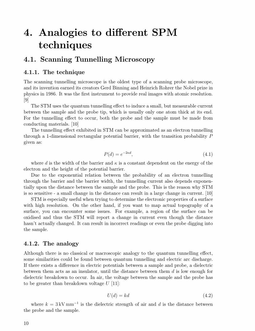
The tunnelling effect exhibited in STM can be approximated as an electron tunnellingthrough a 1-dimensional rectangular potential barrier, with the transition probability Pgiven as:
P (d) = e−2κd, (4.1)
where d is the width of the barrier and κ is a constant dependent on the energy of theelectron and the height of the potential barrier.
Due to the exponential relation between the probability of an electron tunnellingthrough the barrier and the barrier width, the tunnelling current also depends exponen-tially upon the distance between the sample and the probe. This is the reason why STMis so sensitive - a small change in the distance can result in a large change in current. [10]
STM is especially useful when trying to determine the electronic properties of a surfacewith high resolution. On the other hand, if you want to map actual topography of asurface, you can encounter some issues. For example, a region of the surface can beoxidised and thus the STM will report a change in current even though the distancehasn’t actually changed. It can result in incorrect readings or even the probe digging intothe sample.
4.1.2. The analogy
Although there is no classical or macroscopic analogy to the quantum tunnelling effect,some similarities could be found between quantum tunnelling and electric arc discharge.If there exists a difference in electric potentials between a sample and probe, a dielectricbetween them acts as an insulator, until the distance between them d is low enough fordielectric breakdown to occur. In air, the voltage between the sample and the probe hasto be greater than breakdown voltage U [11]:
U(d) = kd (4.2)
where k = 3kVmm−1 is the dielectric strength of air and d is the distance betweenthe probe and the sample.
10
4. ANALOGIES TO DIFFERENT SPM TECHNIQUES
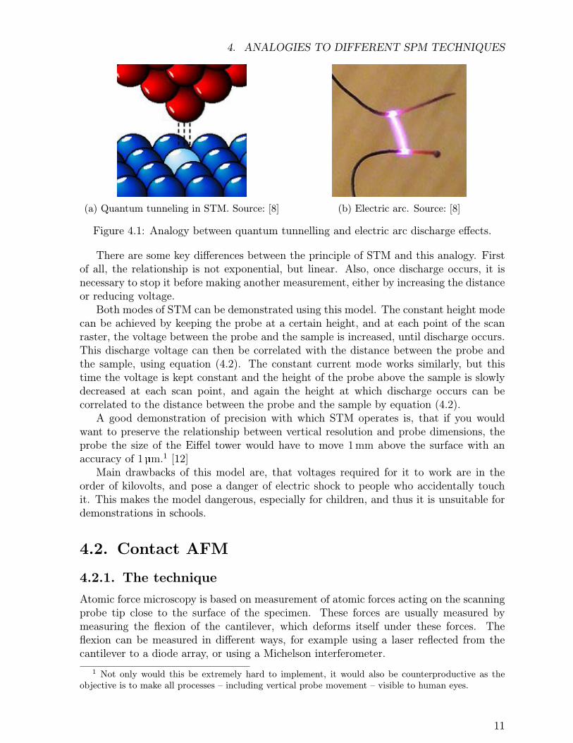
(a) Quantum tunneling in STM. Source: [8] (b) Electric arc. Source: [8]
Figure 4.1: Analogy between quantum tunnelling and electric arc discharge effects.
There are some key differences between the principle of STM and this analogy. Firstof all, the relationship is not exponential, but linear. Also, once discharge occurs, it isnecessary to stop it before making another measurement, either by increasing the distanceor reducing voltage.
Both modes of STM can be demonstrated using this model. The constant height modecan be achieved by keeping the probe at a certain height, and at each point of the scanraster, the voltage between the probe and the sample is increased, until discharge occurs.This discharge voltage can then be correlated with the distance between the probe andthe sample, using equation (4.2). The constant current mode works similarly, but thistime the voltage is kept constant and the height of the probe above the sample is slowlydecreased at each scan point, and again the height at which discharge occurs can becorrelated to the distance between the probe and the sample by equation (4.2).
A good demonstration of precision with which STM operates is, that if you wouldwant to preserve the relationship between vertical resolution and probe dimensions, theprobe the size of the Eiffel tower would have to move 1mm above the surface with anaccuracy of 1 µm.1 [12]
Main drawbacks of this model are, that voltages required for it to work are in theorder of kilovolts, and pose a danger of electric shock to people who accidentally touchit. This makes the model dangerous, especially for children, and thus it is unsuitable fordemonstrations in schools.
4.2. Contact AFM
4.2.1. The technique
Atomic force microscopy is based on measurement of atomic forces acting on the scanningprobe tip close to the surface of the specimen. These forces are usually measured bymeasuring the flexion of the cantilever, which deforms itself under these forces. Theflexion can be measured in different ways, for example using a laser reflected from thecantilever to a diode array, or using a Michelson interferometer.
1 Not only would this be extremely hard to implement, it would also be counterproductive as theobjective is to make all processes – including vertical probe movement – visible to human eyes.
11

4.2. CONTACT AFM
These atomic forces are often approximated by the Lennard-Jones potential, whichcombines attractive van der Waals and repulsive quantum-mechanical interactions [5]:
w(r) = 4w0
[(σr
)12−(σr
)6], (4.3)
where r is the distance between atoms of the surface and the tip, w0 is the minimalvalue of potential energy and σ is the equilibrium distance of the two atoms. By takingthe negative derivative of this potential with respect to distance, we obtain the force ofthis interaction:
F = −dw
dr= 24w0
(2σ12
r13− σ6
r7
). (4.4)
Figure 4.2: Lennard-Jones potential and its interaction force for two atoms. Approximateareas of operation of different AFM modes are marked by dashed rectangles. Vertical axisunits are arbitrary.
In contact mode, the tip is in permanent contact with the specimen, and the forcesacting on it are repulsive and relatively big (in the order of 10−7N). From measurementof these forces, either in constant force mode, or constant height mode, topography of thespecimen can be determined.
12

4. ANALOGIES TO DIFFERENT SPM TECHNIQUES
4.2.2. The analogy
Analogy to contact AFM mode is quite straightforward. The whole system is simplyupscaled, and the probe comes into direct contact with the specimen. Flexion of thecantilever is measured, and correlated with height of the sample at point of contact. Bothconstant force mode and constant height mode can be easily demonstrated.
Figure 4.3: Demonstration of contact mode of AFM.
4.3. Non-contact AFM
4.3.1. The technique
In non-contact AFM mode, the tip of the probe never comes into contact with the sample.Instead, the tip of the probe oscillates at or close to its resonant frequency at a distanceof 50 − 100 A. The attractive van der Waals forces at this distance are in the order of10−9N [5]. These forces, which act on the oscillating probe, cause changes in resonantfrequency, amplitude and phase of the oscillations. These changes can be detected anddistance of the probe and sample can be determined.
Its advantage is low risk of damage, because the sample and the probe never come intocontact. On the other hand, measurements can be affected by presence of a contaminationlayer on the surface of the sample, which can fill in nanostructures and make them harderto detect, or cause other unwanted forces (i.e. viscosity). [5]
This technique can be also applied to other than van der Waals forces, for exampleelectrostatic, magnetic or chemical interactions .
4.3.2. The analogy
Finding an analogy to this method is problematic for several reasons. You have to find asuitable force which acts over macroscopic distances (in the order of centimetres). Grav-itational force is too weak to be detectable. Electrostatic or magnetic force are goodcandidates, but both have drawbacks.
In case of the electrostatic force, both the sample and the tip have to be electricallycharged, which brings problems already mentioned in Section 4.1.2. With magnetic force,
13

4.4. SEMICONTACT AFM (TAPPING MODE)
finding materials with suitable magnetic properties for the probe and the sample can beproblematic, especially in close vicinity of unshielded electronic equipment which can bedamaged. In both cases, the oscillating probe would cause electromagnetic induction dueto Faraday’s law, which would also have to be taken into account.
4.4. Semicontact AFM (tapping mode)
4.4.1. The technique
Semicontact AFM mode combines features of previous two modes. The probe oscillatesas in non-contact mode, but comes into contact with the sample in each cycle. Its benefitsare, that vertical movement of the probe almost completely eliminates lateral forces andthus reduces the risk of probe or specimen damage as opposed to contact mode. Further-more, every cycle it breaches the contamination layer, and allows for direct measurementsof the sample surface. These two properties explain the popularity of semicontact AFM [5].
Figure 4.4: Semicontact mode of AFM (constant amplitude mode).
In this mode, the probe oscillates with a large amplitude (10−100 nm). When it comesinto contact with the sample, this amplitude is reduced, and additionally, the oscillationsare phase-shifted. Both the amplitude change and phase shift can be used to determineproperties of the sample.
4.4.2. The analogy
Semicontact AFM mode is arguably easier to implement in a macroscopic model. Oscil-lations of the cantilever, although at much lower frequencies due to increased dimensions,can be invoked in various ways, such as using a sound speaker, or an electrical coil anda magnet, etc. The oscillating tip will literally tap the surface, which will cause bothchange in amplitude and phase shift.
14

5. OBJECTIVES
5. ObjectivesThe objective of this thesis is to improve the already existing model of a scanning
probe microscope, built at the Institute of Physical Engineering of Brno University ofTechnology, with the purpose of easier and more interesting demonstration of SPM tech-niques to the general public at science fairs and similar events. This objective can be splitinto two separate tasks:
1. Implement a new suitable SPM technique into the model.2. Remove the need for a computer with special software by integrating a single-board
computer into the model.
5.1. New SPM technique implementation
Since the model only supported constant height AFM contact mode (described in Section4.2), it would be beneficial to implement a way to also demonstrate the difference betweenconstant height and constant interaction modes described in Section 2.4. For this, theprobe is needed to be able to move vertically, which requires considerable changes in bothconstruction and electronics of the model.
If this technique is implemented successfully, the model can be further modified tosupport semicontact mode described in Section 4.4. This will also require a way to induceoscillations of the cantilever.
5.2. Single-board computer integration
The model was originally developed to be controlled by an external computer runningWindows OS, so its controlling software was programmed in C# and .NET user environ-ment. This is unfortunately unsuitable for a single-board computer, since these are notable to natively run .NET software.1
This means that the control software has to be ported to a different, preferably moreopen and flexible language.
1 With the introduction of Windows 10 to Raspberry Pi model 2, this may change in the future. Anopen-source alternative (Mono) of course exists, but is not complete and often unreliable.
15

6. FunctionOriginal function schematic of the SPM model is described in Figure 6.1.
Control Unit
X,Y,Z data
X,Y movement
USB serialinterface
Data collectionData plottingUser control
Windows OS PC
Hall Probe
ADC
Z data
Linear X,Y motors
X,Y data
Figure 6.1: Schematic of the original model. A Windows OS computer with controlsoftware installed communicates via a USB serial interface with the Control unit, whichcontrols movement of the sample under the probe and gathers information of probe heightfrom the Hall probe.
This relatively simple design had to be innovated to allow implementations of multiplescanning modes, which require movement of cantilever in vertical axis and induction ofoscillations of the cantilever. Schematic of new design of the model is depicted in Figure6.2.
16

6. FUNCTION
Control Unit
X,Y,Z data
X,Y movement
USB serialinterface
Data collectionData plottingUser control
Raspberry Pi B+
ADC
Z data
Linear X,Y motors
X,Y data
Tensometricarray
ADC
DAC
Oscillation unit
Coil + magnetoscillations
Cantilever flexion (CM)Climber height (sCM)
Z movement StepperMotor
GPIO serialinterface
Scan ModeSet Point
Display+
Input
Figure 6.2: Schematic of the new model. All innovated components are marked in blue.Both custom printed circuit boards (PCBs) are controlled by a Raspberry Pi computervia serial communication interfaces. A new Oscillation unit was implemented to gatherand analyse data from a tensometric array placed on the cantilever and control oscillationsand vertical movement of the cantilever. This data is analysed, and afterwards sent tothe control unit,1 which combines it with information about position of sample and sendsit to the Raspberry Pi computer, where it can be plotted and displayed.
1This ensures that there is minimal time delay between gathering Z data and combining it with Xand Y data. Were the information sent directly to the Raspberry Pi, then the data would be sent via twodifferent serial interfaces, not one. This could cause additional and unpredictable delays between signalsin input/output buffers of these serial ports.
17
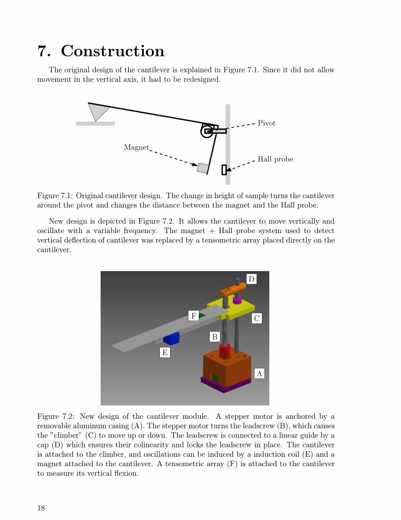
7. ConstructionThe original design of the cantilever is explained in Figure 7.1. Since it did not allow
movement in the vertical axis, it had to be redesigned.
Pivot
Magnet
Hall probe
Figure 7.1: Original cantilever design. The change in height of sample turns the cantileveraround the pivot and changes the distance between the magnet and the Hall probe.
New design is depicted in Figure 7.2. It allows the cantilever to move vertically andoscillate with a variable frequency. The magnet + Hall probe system used to detectvertical deflection of cantilever was replaced by a tensometric array placed directly on thecantilever.
E
D
C
B
A
F
Figure 7.2: New design of the cantilever module. A stepper motor is anchored by aremovable aluminum casing (A). The stepper motor turns the leadscrew (B), which causesthe ”climber” (C) to move up or down. The leadscrew is connected to a linear guide by acap (D) which ensures their colinearity and locks the leadscrew in place. The cantileveris attached to the climber, and oscillations can be induced by a induction coil (E) and amagnet attached to the cantilever. A tensometric array (F) is attached to the cantileverto measure its vertical flexion.
18

7. CONSTRUCTION
C
B
A
ED
Figure 7.3: Photo of the new model. A - control unit, B - oscillation unit, C - RaspberryPi, D - cantilever module, E - sample.
19

8. ElectronicsThe original model contained one custom-designed PCB (the control unit) for con-
trol and data collection. In the new design, one additional custom-designed PCB (theoscillation unit) and a Raspberry Pi model B+ single-board computer were implemented.
8.1. Oscillation unit
8.1.1. Function
An overview of the oscillation unit function is given in Figure 6.2. Just as the controlunit, it is powered by an Atmega8 microcontroller and programmed in C programminglanguage. It enables following functions:
• Scan mode selection - CM/sCM, CHM/CIM.1
• Vertical movement of cantilever.• Induction of oscillations of cantilever with variable frequency and precision of ±0,1Hz.• Feedback loop for constant interaction mode - see Table 8.1.• Gathering, processing and sending data - see Table 8.2.
8.1.2. Oscillations and feedback
Table 8.1: Set point variables in individual scanning modes.
CHM CIM
CM –Cantileverdeflection
sCM –Oscillationamplitude
Table 8.2: Variables for data processing and plotting. These are the variables which aresent to the control unit as Z data.
CHM CIM
CM Cantileverdeflection
Climberheight
sCM Oscillationamplitude
Climberheight
1For explanation of these individual modes, refer to Sections 2.4, 4.2 and 4.4.
20

8. ELECTRONICS
Both extraction of oscillation amplitude from the signal from the tensometers and alsofeedback loop for constant interaction mode could be implemented either using electricalcircuits or digitally. For purposes of this model, purely digital implementation was used.The reasons are following:
Extraction of oscillation amplitude from the signal could be carried out by an electroniccircuit called the envelope detector – Figure 8.1. The time constant τ = RC of this circuithas to be tuned to suit the cantilever’s oscillation frequency. In general, the time constantmust fulfil the following equation [13]:
1
fm� τ � 1
fc, (8.1)
where fm is the highest modulation frequency of the signal (i.e. how fast the signalamplitude is changing), and fc is the carrier frequency of the signal (i.e. frequency ofcantilever oscillations). This means that if the cantilever is for any reason changed forone with a different oscillation frequency, this circuit would also have to be modified.Implementing envelope detection digitally is thus beneficial to flexibility of the model.
Input Output
Figure 8.1: Envelope detector circuit schematic.
A feedback loop circuit would be much more complicated, since the stepper motorrequires very specific values and characteristics of signals at each of its input wires. Con-trolling the feedback digitally makes it much easier to modify and again benefits theflexibility of the model.
8.2. Raspberry Pi Model B+
8.2.1. Function
The single-board computer integrated into the model is required for following tasks:
• Communication with and control of both custom PCBs (control and oscillation unit)via serial interfaces.
• Collection and analysis of recieved data.• User control and data display in a graphical user interface.
All these tasks were originally carried out by the external Windows OS computer.After integration of the Raspberry Pi, only an external display and mouse+keyboardconnection is required.2 Controlling the device with a laptop (or a smartphone) is still
2Both of these devices can be also easily integrated into the model, at an estimated cost from 3000,-CZK upwards.
21
8.2. RASPBERRY PI MODEL B+
possible using a wireless or Ethernet connection and a VNC (Virtual Network Computing)program.
8.2.2. Software
Control software for the device was originally written in C#. This, as mentioned inSection 5.2, is unsuitable for Raspberry Pi. A different language, Python, was chosen forfollowing reasons:
• It is a completely open language with a large user base.• Its syntax is easy to learn and read – it is often recommended as a good first
programming language for beginners.• It is well-integrated with Linux and Raspberry Pi.• It is an interpreted language – it does not require compilation before running and
is easy to debug at runtime.• Its large and powerful libraries (NumPy, SciPy, matplotlib) make it easy to analyse
and visualise collected data.
Python also has its drawbacks, the most important one being speed. While it is stillwell-optimised, Python code cannot match similar code in C or other low-level languages.Fortunately, the Raspberry Pi Model B+ offers enough computational power to allow itsuse in this project.
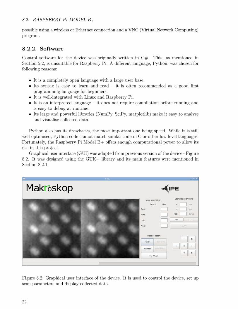
Graphical user interface (GUI) was adapted from previous version of the device - Figure8.2. It was designed using the GTK+ library and its main features were mentioned inSection 8.2.1.
Figure 8.2: Graphical user interface of the device. It is used to control the device, set upscan parameters and display collected data.
22

9. CANTILEVER OSCILLATIONS
9. Cantilever oscillationsOscillation frequency of the cantilever is an important variable in every semicontact
and noncontact AFM.
9.1. Free cantilever oscillations
Motion of a fixed-free oscillating cantilever (Figure 9.1) can be described with a fourth-order time-dependent partial differential equation [14]:
EI∂4y
∂x4+ ρA
∂2y
∂t2= 0, (9.1)
where y(x, t) is the transverse deflection of the cantilever, E is the Young module ofthe cantilever, I is area moment of inertia, ρ is cantilever density and A is cantilevercross-section area.
w
t
L
y
x
Figure 9.1: Fixed-free oscillating cantilever.
Solving this equation (for example in [15]) gives rise to these natural cantilever fre-quencies:
ωn = An
√EI
µL4, (9.2)
where L is cantilever length, n is the number of oscillation mode, and An is a constant.For a fixed-free cantilever, values of A for first 3 modes are A1 = 3.52, A2 = 22.0 andA3 = 61.7 [15].
By inserting cantilever dimensions and material characteristics into equation (9.2), werecieve the following resonance frequency:
f1 =A1
2π
√EI
µL4=A1
2π
√Et2
12ρL4=
3.52
2π
√2.1× 1011 Pa× 0.49mm2
12× 7850 kgm−3 × 53.1 dm4 ≈ 8.0Hz (9.3)
23

9.2. CANTILEVER AS A DRIVEN DAMPED HARMONIC OSCILLATOR
9.2. Cantilever as a driven dampedharmonic oscillator
If there are external forces acting on the cantilever, an additional term appears on theright side of equation (9.1). Solutions of this equation depend on characteristics of theexternal force and aren’t trivial [16].
Instead, the cantilever can be modelled as a driven damped harmonic oscillator. Itsequation of motion then becomes:
d2y
dt2+ 2γ
dy
dt+ ω2
0y = f(t), (9.4)
where ω0 is the natural resonance frequency, γ is the damping factor and f(t) is thedriving force as a function of time.
9.2.1. Sinusoidal wave
Usually, the driving force has a sinusoidal shape:
f(t) = C sin(ωt), (9.5)
where C is the amplitude and ω is the angular frequency of the driving force. The equation(9.4) can then be solved analytically [17], and the resonance curve1 is displayed in Figure9.3.
9.2.2. Square wave
In our model, time dependence of the driving force has the shape of a square wave - seeFigure 9.2. A square wave with an amplitude C can be represented via a Fourier seriesas a linear combination of sinusoidal waves and a constant term:
f(t) = C
(1
2+
2
π
∞∑n=1,3,5...
sin(nωt)
n
), (9.6)
The differential equation (9.4) becomes:
d2y
dt2+ 2γ
dy
dt+ ω2
0y =F0
2+
2F0
π
∞∑n=1,3,5...
sin(nωt)
n, (9.7)
where F0 is the amplitude of the driving force. A resonant response from the oscillatorshould occur each time when the frequency ωn = nω, n = 1, 3, 5... of one of terms fromthe sum is close to or equal to the resonant frequency ω0 of the oscillator [18].
Resonance curves for a harmonic oscillator driven by a sinusoidal or a square wave– calculated using a numerical simulation – are displayed in Figure 9.3. The resonanceresponse of cantilever used in the model is displayed in Figure 9.4.
1Dependence of steady-state oscillations amplitude on frequency of driving force.
24

9. CANTILEVER OSCILLATIONS
t
f(t)
Figure 9.2: A square wave with its 4 most significant components (constant term, funda-mental sine wave, third and fifth harmonics).
Figure 9.3: Resonance curves for a sinusoidal and square-wave driving force. Verticalaxis units are arbitrary. f0 = 7Hz. Notice the extra peaks corresponding to resonancewith higher hamonics of the square wave (f = f0
n, n = 1, 3, 5, ...), which are absent in the
resonance curve for a sinusoidal force.
25

9.2. CANTILEVER AS A DRIVEN DAMPED HARMONIC OSCILLATOR
Figure 9.4: Measured resonance curve of the cantilever. Resonant frequency f0 = 8.7Hz.Extra peaks at frequencies (f = f0
n, n = 1, 3, 5, ...) are present, just as the numerical model
predicted.
26

10. NOTABLE FEATURES
10. Notable features10.1. Development process
The development process of the model resembles in many ways development processes ofactual scanning probe microscopes. First STMs and AFMs were contact mode (devel-oped in 1981, resp. 1986) [19]. Noncontact AFM and semicontact AFM were developedsubsequently in the next decade [20]. In our model, contact mode was also first to bedeveloped, with semicontact mode implemented additionally.
10.2. Signal path
Another interesting similarity can be found in the design of oscillation unit. Between thecantilever and final display in the computer, the signal changes form between analog anddigital several times using analog/digital and digital/analog converters (ADC and DAC)– see Figure 10.1. At first, the control unit received data directly from the probe, butlater the data is first processed by the oscillation unit and then sent to the control unit.Similar features can be found in real AFMs: The Oscillation Controller 4 by companySpecs Zurich also takes analog inputs and can produce analog outputs, but all internaldata processing is purely digital:
“With an analog bandwidth of 5 MHz the OC4 is wellsuited to operating athigher resonance modes. [. . .] Internal signals are represented at 32 bits withat least 1 MS/s. [. . .] Up to six analog outputs and two digital lines allow easyintegration with any SPM controller.” [21]
TensometersOperationalAmplifier ADC
OscillationUnit
DAC
ADCControlUnit
Raspberry Pi
A A A
A
D D
D D
Figure 10.1: Path of signal from the cantilever to the Raspberry Pi computer. Signalchanges form between analog (A) and digital (D) multiple times.
27
11. ConclusionPurpose of this work was to improve an already-existing model of a scanning probe
microscope by researching and implementing an additional suitable SPM technique, andremoving the need for an external computer by implementing a single-board computerinto the device.
Originally, the model only supported constant height contact mode of SPM. Afterresearching and discussing multiple options, the model was modified to support four dif-ferent SPM techniques – constant height and constant interaction mode, both of which canrun in contact or semicontact mode. In Chapter 9, behaviour of oscillating cantilever wasstudied, with interesting results arising from simple analysis techniques such as harmonicapproximation and Fourier analysis.
A single-board computer – Raspberry Pi model B+ – was implemented into the device.An external computer is now no longer necessary, although external input devices (mouseand keyboad) and output devices (display) are still required for operation. Use of open-source systems and popular programming languages made the device more flexible anduser-friendly. Many features – for example enhanced data analysis or an analogy toindividual atom manipulation – can be implemented in the future.
This model can not only serve as a great demonstration tool on science fairs andpopular science lectures. It can also be useful to somebody, who wants to improve theirpractical skills such as programming, construction or designing electronic circuits. Theycan practice their knowledge and try out new ideas on a functional device without riskingmajor damage or high production costs. This practical experience, which many scien-tists lack, can be invaluable later in their career, when they will be designing their ownexperiments and instruments.
28

BIBLIOGRAPHY
Bibliography[1] BOTTOMLEY, L. A.: Scanning probe microscopy. Analytical Chemistry, vol. 70,
no. 12, 1998, p. 425R–475R. ISSN 0003-2700
[2] VUJTEK, M, KUBINEK, R, MASLAN, M.: Nanoskopie. Palacký University Olo-mouc, 2012, 122 p. ISBN 978-80-244-3102-4
[3] LAPSHIN, R. V.: Feature-oriented scanning probe microscopy. Encyclopedia ofNanoscience and Nanotechnology, vol. 14, 2011, p. 105–115. ISSN 0957-4484
[4] ASHBY W. R.: An Introduction to Cybernetics, Chapman & Hall, London, 1956.Internet (1999): <http://pcp.vub.ac.be/books/IntroCyb.pdf>
[5] EATON, P, WEST, P.: Atomic Force Microscopy. Oxford University Press, Inc.,2010, 257 p. ISBN 978-01-995-7045-4
[6] LORENZ, J. K. et al.: A refrigerator magnet analog of scanning-probe microscopy.Journal of Chemical Education, vol. 74, no. 9, 1997, p. 1032. ISSN 0021-9584
[7] QUARDOKUS, R. C, WASIO, N. A. and KANDEL, S. A.: The Scanning ThereminMicroscope: A model scanning probe instrument for hands-on activities. Journal ofChemical Education, vol. 91, no. 2, 2014, p. 246–250. ISSN 0021-9584
[8] Wikimedia Commons articles: Theremin, Scanning Tunneling Microscopy, Electricarc. <https://commons.wikimedia.org/>, Accessed: 2015-05-08.
[9] BINNIG, G, ROHRER, H.: Scanning tunneling microscopy. Surface Science, vol.126, 1983: p. 236–244. ISSN 0039-6028
[10] HANSMA, P, TERSOFF, J.: Scanning tunneling microscopy. Journal of AppliedPhysics, vol. 61, no. 2, 1987: p. R1–R24. ISSN 0021-8979
[11] TIPLER, P. A.: College Physics. Worth Publishers, Inc., 1987, 932 p. ISBN 978-08-790-1268-7
[12] RIEDER, K.: STM - manipulation of atoms and molecules. <http://www.fzu.cz/~nanoteam/events/ws2006/rieder.pdf>, Accessed: 2015-03-15.
[13] LESURF, J.: The Scots Guide to Electronics. <https://www.st-andrews.ac.uk/~www_pa/Scots_Guide/RadCom/intro.html>, Accessed: 2015-05-08.
[14] RABE, U, TURNER, J. and TURNER, W. A.: Analysis of the high-frequency re-sponse of atomic force microscope cantilevers. Applied Physics A - Materials Science& Processing, vol. 66, no. 1, 1998, p. S277–S282. ISSN 0947-8396
[15] HARRIS, C. M.: Shock and Vibration Handbook, 5th Edition. McGraw-Hill, 2002,1456 p. ISBN 0-07-137081-1
[16] SADER, J.: Frequency response of cantilever beams immersed in viscous fluids withapplications to the atomic force microscope. Journal of Applied Physics, vol. 84,no. 1, 1998, p. 64–76. ISSN 0021-8979
29

BIBLIOGRAPHY
[17] Harvard University: Forced Damped Harmonic Oscillators. <http://isites.harvard.edu/fs/docs/icb.topic251677.files/notes23.pdf>, Accessed: 2015-05-10.
[18] BUTIKOW, E. I.: Square-wave excitation of a linear oscillator. American Journal ofPhysics, vol. 72, no. 4, 2004, p. 469–476. ISSN 0002-9505
[19] BINNIG, G, QUATE, C. F.: Atomic force microscope. Physical Review Letters,vol. 56, no. 9, 1986, p. 930–934. ISSN 0003-6951
[20] ZHONG, Q. et al.: Fractured polymer/silica fiber surface studied by tapping modeatomic force microscopy. Surface science, vol. 290, no. 1, 1993, p. L688–L692. ISSN0039-6028
[21] Specs Zurich. Oscillation Controller 4 product brochure. <http://www.specs-zurich.com/upload/cms/user/OC4ProductBrochure.pdf>, Accessed:2015-05-09.
30

List of acronyms• ADC – analog-to-digital converter• AFM – atomic force microscopy• CHM – constant height mode• CIM – constant interaction mode• CM – contact mode• DAC – digital-to-analog converter• GUI – graphical user interface• MFM – magnetic force microscopy• OS – operating system• PCB – printed circuit board• sCM – semicontact mode• SCM – scanning capacitance microscopy• SNOM – scanning near-field optical microscopy• SPM – scanning probe microscopy• STM – scanning tunnelling microscopy• SThM – Scanning Theremin Microscope• VNC – Virtual Network Computing