Vol.15, January.2015 ISSN 2354-7065 - isomase.orgisomase.org/JOMAse/Vol.15 Jan 2015/Vol-15.pdf · Buana Ma’ruf (Badan Pengkajian dan Penerapan Teknologi, Indonesia) ... The equation

ISSN 2354-7065Vol.15, January.2015

Journal of Ocean, Mechanical and Aerospace -Science and Engineering-

Vol.15: January 2015

ISOMAse

International Society of Ocean, Mechanical and Aerospace -Scientists and Engineers-

Contents

About JOMAse

Scope of JOMAse

Editors

Title and Authors PagesWake Oscillator Model for Vortex-Induced Vibrations Predictions on Low Aspect Ratio Structures

Mohd Asamudin A Rahman, Krish Thiagarajan, Jeremy Leggoe, Ahmad Fitriadhy

1 - 6

Initial Imperfection Design of Subsea Pipeline to Response Buckling Load

Abdul Khair Junaidi, Jaswar Koto

7 - 11

Effect of Bending and Straightening to the Strength of Reinforcement Steel Bar

Kana Sabatul Ikhwan, M.Dalil

12 - 17

The Floating Production, Storage and Offloading Vessel Design for Oil Field Development in Harsh Marine Environment

Ezebuchi Akandu, Atilla Incecik, Nigel Barltrop

18 - 24



ISOMAse


About JOMAse

The Journal of Ocean, Mechanical and Aerospace -science and engineering- (JOMAse, ISSN: 2354-7065) is an online professional journal which is published by the International Society of Ocean, Mechanical and Aerospace -scientists and engineers- (ISOMAse), Insya Allah, twelve volumes in a year. The mission of the JOMAse is to foster free and extremely rapid scientific communication across the world wide community. The JOMAse is an original and peer review article that advance the understanding of both science and engineering and its application to the solution of challenges and complex problems in naval architecture, offshore and subsea, machines and control system, aeronautics, satellite and aerospace. The JOMAse is particularly concerned with the demonstration of applied science and innovative engineering solutions to solve specific industrial problems. Original contributions providing insight into the use of computational fluid dynamic, heat transfer, thermodynamics, experimental and analytical, application of finite element, structural and impact mechanics, stress and strain localization and globalization, metal forming, behaviour and application of advanced materials in ocean and aerospace engineering, robotics and control, tribology, materials processing and corrosion generally from the core of the journal contents are encouraged. Articles preferably should focus on the following aspects: new methods or theory or philosophy innovative practices, critical survey or analysis of a subject or topic, new or latest research findings and critical review or evaluation of new discoveries. The authors are required to confirm that their paper has not been submitted to any other journal in English or any other language.



ISOMAse


Scope of JOMAse

The JOMAse welcomes manuscript submissions from academicians, scholars, and practitioners for possible publication from all over the world that meets the general criteria of significance and educational excellence. The scope of the journal is as follows:

• Environment and Safety • Renewable Energy • Naval Architecture and Offshore Engineering • Computational and Experimental Mechanics • Hydrodynamic and Aerodynamics • Noise and Vibration • Aeronautics and Satellite • Engineering Materials and Corrosion • Fluids Mechanics Engineering • Stress and Structural Modeling • Manufacturing and Industrial Engineering • Robotics and Control • Heat Transfer and Thermal • Power Plant Engineering • Risk and Reliability • Case studies and Critical reviews

The International Society of Ocean, Mechanical and Aerospace –science and engineering is inviting you to submit your manuscript(s) to [email protected] for publication. Our objective is to inform authors of the decision on their manuscript(s) within 2 weeks of submission. Following acceptance, a paper will normally be published in the next online issue.



ISOMAse


Editors

Chief-in-Editor

Jaswar Koto (Ocean and Aerospace Research Institute, Indonesia Universiti Teknologi Malaysia, Malaysia)

Associate Editors

Abyn Hassan (Persian Gulf University, Iran) Adhy Prayitno (Universitas Riau, Indonesia) Adi Maimun (Universiti Teknologi Malaysia, Malaysia) Agoes Priyanto (Universiti Teknologi Malaysia, Malaysia) Ahmad Fitriadhy (Universiti Malaysia Terengganu, Malaysia) Ahmad Zubaydi (Institut Teknologi Sepuluh Nopember, Indonesia) Ali Selamat (Universiti Teknologi Malaysia, Malaysia) Buana Ma’ruf (Badan Pengkajian dan Penerapan Teknologi, Indonesia) Carlos Guedes Soares (Centre for Marine Technology and Engineering (CENTEC), University of Lisbon, Portugal) Dani Harmanto (University of Derby, UK) Iis Sopyan (International Islamic University Malaysia, Malaysia) Jamasri (Universitas Gadjah Mada, Indonesia) Mazlan Abdul Wahid (Universiti Teknologi Malaysia, Malaysia) Mohamed Kotb (Alexandria University, Egypt) Priyono Sutikno (Institut Teknologi Bandung, Indonesia) Sergey Antonenko (Far Eastern Federal University, Russia) Sunaryo (Universitas Indonesia, Indonesia) Tay Cho Jui (National University of Singapore, Singapore)

Published in Indonesia.

ISOMAse, Jalan Sisingamangaraja No.89 Pekanbaru-Riau Indonesia http://www.isomase.org/

Printed in Indonesia.

Teknik Mesin Fakultas Teknik Universitas Riau, Indonesia http://ft.unri.ac.id/

Journal of Ocean, Mechanical and Aerospace -Science and Engineering-, Vol. 15

January 20, 2015

1 Published by International Society of Ocean, Mechanical and Aerospace Scientists and Engineers

Wake Oscillator Model for Vortex-Induced Vibrations Predictions on Low Aspect Ratio Structures

Mohd Asamudin A Rahman,a,b* Krish Thiagarajan,c Jeremy Leggoe,a and Ahmad Fitriadhy,b

a)School of Mechanical Engineering, University of Western Australia, Crawley, WA, Australia b)School of Ocean Engineering, Universiti Malaysia Terengganu, Terengganu, Malaysia c)Department of Mechanical Engineering, University of Maine, Orono, USA *Corresponding author: [email protected] Paper History Received: 29-December-2014 Received in revised form: 14-January-2015 Accepted: 19-January-2015

ABSTRACT A phenomenological Wake Oscillator Model (WOM) is studied to capture the coupling effects between the fluid and the structure. The Vortex-Induced Vibration (VIV) phenomenon is modelled to describe the motion imposed by the lift forces on the structure. The influence of the aspect ratio (L/D) was introduced into the model to characterize the VIV phenomenon for finite cylinders. The proposed model captured the basic features of the VIV such as the amplitude of vibration, frequency, and lift coefficient by coupling the structural equation to the wake equation. Predictions of the WOM are discussed and compared with the experimental data in order to establish a relationship describing VIV as a factor of aspect ratios. KEY WORDS: Vortex-Induced Vibrations; Wake Oscillator Model, circular cylindrical structure; aspect ratio effects 1.0 WAKE OSCILLATOR MODEL Offshore structures such as jacket platform, risers, mooring lines, Spars, and pipelines, are subject to severe climate and ocean conditions. These structures undergo unremitting forces from the current or wave which resulting in fatigue due to vibration. One of the identified problem is due to Vortex-Induced Vibrations (VIV). VIV is a phenomenon in a fluid flow caused by the shedding of vortices behind the structures due to the interactions

of fluid and structure. Comprehensive review have been done by King [1], Sarpkaya [2], Bearman [3], Pantazopolous [4], Williamson and Govardhan [5], and books of Chen [6], Blevins [7], and Sumer and Fredsoe [8], to name a few.

Studies of the VIV have been carried out using different approaches such as experiments, numerical and analytical study. Each one of the approach contribute significantly to the expansion of the knowledge in prediction of VIV. In the present study, the main interest is on Wake Oscillator Model (WOM), as a semi-empirical model for a prediction of the VIV phenomenon in a fluid flow. There are three main types of semi-empirical model, as summarized by Gabbai and Benaroya [9] which are, Wake-body coupled models or wake oscillator model (WOM), Single degree of freedom models (SDOF), and Force decomposition models.

Bishop and Hassan [10], Hartlen and Currie [11], Skop and Griffin [12], Iwan and Blevins [13], Landl [14], Griffin [15], Facchinetti et al. [16] are among the contributors to the development of WOM. Meanwhile, Simiu and Scanlan [17], Goswami et al. [18] use SDOF models to describe the behaviour of the structural oscillator. Sarpkaya [19] is credited for the force decomposition models and succeeded later by Griffin and Koopman [20].

The prediction models are based on the equation of motion of a flexible mounted structure in the transverse direction with 2D flow as defined by [8]. The equation for a single degree of freedom system can be generally written as:

Mass term + Damping term + Stiffness term = Forcing term

+ + = (1)

where m is the total mass of the system, c is the structural damping, k is spring stiffness, y is the cross-flow displacement and F is the forcing term. A dot over the symbols denotes differentiation with respect to time. This equation is known as

Journal of Ocean, Mechanical and Aerospace-Science and Engineering-, Vol. 15

2 Published by International Society of Ocean, Mechanical and Aerospace

structure oscillator. Figure 1 shows a schematic diagram for an elastically supported rigid cylinder.

Figure 1: Elastically supported rigid cylinder

Birkhoff and Zarantanello [21] first

called wake oscillator in order to determine the vortex shedding frequency by theoretical formula. Following this pioneering contribution, numerous works have proposed solving VIV problems by analytical approaches. Bishop and Hassan suggested representing the time-varying forces on a cylinder due to vortex shedding by using a van der Pol type oscillator. Hartlen and Currie [11] proposed a lift oscillator model by coupling the lift force to the cylinder motion (equations satisfies the following characteristics: i. The oscillator should be self-exciting and self

means the lift force in the lock-in region is periodic and infinite.

ii. The natural frequency of the oscillator should be proportional to the uniform flow velocity and coincide with the vortex shedding frequency.

iii. The cylinder motion and the oscillator must be connected dynamically.

Lorrr cayyy ωζ =++ &&& 2

rLoLo

LoL ybcccc &&&&& =++− 23)( ωωγαω

where yr is the dimensionless amplitude,

coefficient, is the damping factor, the frequency ratio, and , , , are parameters defined to best fit the equation to the experimental data. α and γ are the linear and nonlinear term for damping. Both equations were made dimensionless by the following definition; i. Dimensionless displacement

D

yyr =

Journal of Ocean, Mechanical and Aerospace

Published by International Society of Ocean, Mechanical and Aerospace Scientists and Engineers

1 shows a schematic diagram for an

rigid cylinder [13].

introduced a model mine the vortex shedding

frequency by theoretical formula. Following this pioneering contribution, numerous works have proposed solving VIV problems by analytical approaches. Bishop and Hassan [10]

varying forces on a cylinder due to vortex shedding by using a van der Pol type oscillator. Hartlen

proposed a lift oscillator model by coupling the lift force to the cylinder motion (equations (2) and (3)) that

exciting and self-limiting which region is periodic and

The natural frequency of the oscillator should be proportional to the uniform flow velocity and coincide with the vortex

The cylinder motion and the oscillator must be connected

(2)

(3)

is the dimensionless amplitude, is the lift the frequency ratio, and

are parameters defined to best fit the equation to the are the linear and nonlinear term for

damping. Both equations were made dimensionless by the

(4)

ii. Dimensionless time

tm

kt nωτ ==

iii. Damping ratio

nm

c

ωξ

2=

iv. Dimensionless parameter

mS

LDa

t22

2

8πρ=

v. Frequency ratio

==

Df

US

f

f

nt

n

soω

The model captures most of the features of VIV, such as amplitude response, frequency ratiofigure 2, where stable branches of the periodic motions are represented by solid lines, while unstable branches are represented by dotted lines. Hysteresis phenomenon is indicated by arrows on the plots.

Figure 2: Amplitude and frequency response from Hartlenand Currie model

Facchinetti et al. [16] examine three different coupling terms,

namely displacement coupling and acceleration coupling, forcing term, to be coupled with the wake equation.fluctuating lift equation or wake oscillator defined by Nayfeh can be written as:

Fqqqq ff =Ω+−Ω+ &&& )1( 2ε

where q is the dimensionless wake variable, frequency, ɛ is the structure reduced damping and term. The wake oscillator was coupled with the structure oscillator equation by the introduction of dimensionless time and space. It was found that acceleration coupling succeeds best in

January 20, 2015

(5)

(6)

(7)

(8)

The model captures most of the features of VIV, such as amplitude response, frequency ratio and hysteresis as shown in

2, where stable branches of the periodic motions are represented by solid lines, while unstable branches are represented by dotted lines. Hysteresis phenomenon is indicated

Amplitude and frequency response from Hartlen

urrie model [9]

examine three different coupling terms, namely displacement coupling, = , velocity coupling, =

and acceleration coupling, = , where f is defined as the forcing term, to be coupled with the wake equation. The nonlinear

ion or wake oscillator defined by Nayfeh [22]

F

(9)

is the dimensionless wake variable, Ωf is the angular is the structure reduced damping and F is the forcing

term. The wake oscillator was coupled with the structure oscillator equation by the introduction of dimensionless time and

as found that acceleration coupling succeeds best in


January 20, 2015


predicting the VIV response. The stable solution of the acceleration coupling covered most the data collected from the experiments. Meanwhile, the velocity and displacement coupling fails to predict the phase compared to the experimental data.

Due to the complexity of vortex shedding in the near wake region, an exact solution for the fluid structure interaction is yet to be found. Therefore, an approximate model must be constructed to predict the physics of the VIV [13]. However, in most of these wake oscillator models, the 3D effects were not considered [9]. Hence, in this paper, the reliability of the van der Pol equation to capture the 2D phenomenon has been extended to a 3D model with the influence of aspect ratio included for a better prediction of the dynamic response of structures to VIV. To the authors’ knowledge, there are only few studies on effects of L/D have been conducted in water channel for low cylinder aspect ratio (e.g., L/D < 10). For some latest work along this line, see Rahman et al. [23] and Gonçalves et al. [24]. The main objectives in developing this phenomenological model are to validate our VIV experimental data from [23] and to capture any complex behaviour of the VIV phenomenon observed in experiments.

In the present study, a coupled WOM from the literature have been examined to predict the behaviour of the VIV phenomenon and compared with the experimental results. For all aspect ratios, the WOM was solved using the parameters in table 1. Meanwhile, the value of CD and CL over Ur was extracted from the experimental results by Rahman et al. [23].

Table 1: Parameters for aspect ratio examined. (Extracted from Rahman et al. [23])

Symbol L/D L D k m fn ζ St Exp. 1 13 0.78 0.06 245 5.734 0.99 0.031 0.1455 Exp. 2 10 0.6 0.06 245 4.411 1.12 0.031 0.1292

Exp. 3 7.5 0.6 0.08 245 7.841 0.865 0.036 0.1105 Exp. 4 5 0.4 0.08 245 5.228 1.035 0.032 0.0983 Exp. 5 3 0.33 0.11 52 8.154 0.508 0.026 0.1111

Exp. 6 2 0.22 0.11 52 5.436 0.569 0.021 0.1003 Exp. 7 1 0.16 0.16 52 5.926 0.543 0.030 0.0910

Exp. 8 0.5 0.08 0.16 52 4.182 0.695 0.034 0.0670 2.0 Modified Wake Oscillator Model Coupled WOM by Facchinetti et al. [16] was introduced and modified to suit the flow problem, in order to capture the behaviour of the VIV based on the present experimental data. The coupled model considered the aspect ratio effects in the model with the inclusion of a few assumptions and parameters. It should be emphasized that the development of the WOM will not capture the whole behaviour of the VIV. However, the present attempts are to model the VIV phenomenon based on the data obtained in our experiments. Additionally, the attempts are also to interpret some of the behaviour observed in the experiments with the various parameters included in the present WOM.

Facchinetti et al. [16] discussed the importance of coupling effects on the wake oscillator model performance. This provided significant improvements in the WOM from the classical model introduced by Hartlen and Currie [11] and other researchers before. Coupling equations of structure and wake flow from

Facchineti et al. [16] were used to investigate the effects of aspect ratio in the fluid-structure interaction model. The selection of the acceleration coupling term was based on the conclusion given by Facchinetti et al.[16], who succeeded to model the lock in domain for single degree of freedom case. The structure and wake oscillators equations defined by Facchinetti et al. [16] were;

syym

y =+

++ 2

*2 δγξδ &&&

(10)

yAqqqq &&&&& =+−+ )1( 2ε (11)

where ξ is the structure reduced damping, δ is the reduced

angular frequency of the structure, γ is the stall parameter, m* is the mass ratio, and ε and A are tuning parameters.

The dimensionless fluctuating lift force term, s on the RHS of equation (10) is defined as

Mqs = (12)

*8

1

2 22 mSt

CM Lo

π=

(13)

where CLo is the reference lift coefficient, M is the mass

number which scales the effects of the wake on the structure, and q is the fluid variables (refer Fachhinetti et al. [16] for details). In this coupled term, Facchinetti et al.[16] recommended a value of CLo = 0.3 for a large range of Reynolds number (300 < Re < 1.5 × 105). In an attempt to solve the coupled equations for an oscillating cylinder, the value of CLo is chosen as the lift values derived from free oscillating cylinder experimental results instead of reference values for stationary cylinder, as suggested by [16]. The same consideration was applied to the calculation of the stall parameter. The stall parameter, γ is related to the mean sectional drag coefficient of the structure and given by

St

CD

πγ

4=

,

(14)

Facchinetti et al. [16] suggested amplified drag coefficient,

CD = 0.2 to simplify the model, based on the motion in the transverse direction. However, to improve the validity of the model in comparison with the experimental data, the value of CD

in the equation was defined as the mean drag coefficient value acquired from single degree of freedom free oscillating experiments presented in Rahman et al. [23]. Both CLo and CD were varied for each reduced velocity examined. That means the behaviour of the wake can be specifically captured at each Reynolds number by solving the coupled equations.

The coupled system equation was solved using numerical techniques in MATLAB. The parameters used to solve the coupled equations (10) and (11) were derived from experimental results for different L/D by [23]. The equations were solved to capture the structural responses for the aspect ratio investigated. The value of the van der Pol parameter, ε and the scaling of coupling force, A were varied to obtain a best fit with the experimental plot.


January 20, 2015


3.0 RESULTS AND DISCUSSIONS Figure 3 shows a series of the results obtained from solving the coupled equations. Based on the results acquired, it is seen that there was a good agreement between the present coupled models and the experimental values. The WOM captured the response amplitudes of the structure over reduced velocities investigated in the experiments, and established the best fit for varying values of ε and A in each case.

The results comparing the model with the experimental values such as plotted in figure 3. Experiment 8 (L/D = 0.5) in figure 3 (h) shows a higher value of the amplitude response at higher reduced velocities. This is possibly due to three-dimensional effects captured by the present WOM. Note that the Strouhal values used in the present WOM development were derived from the experiments and significantly lower from the published value of St = 0.2.

Figure 3: (a) – (h). Comparisons of present coupled WOM with experimental data for each aspect ratio investigated.

2 3 4 5 6 7 8 9 10 11 120

0.2

0.4

0.6

0.8

1

1.2

1.4

Ay/D

Ur

WOM (A=0.4, ε = 0.55)Experiment 1(L/D = 13)

2 4 6 8 10 12 140

0.2

0.4

0.6

0.8

1

1.2

1.4

Ay/D

Ur


2 4 6 8 10 12 140

0.2

0.4

0.6

0.8

1

1.2

1.4

Ay/D

Ur


2 4 6 8 10 12 140

0.2

0.4

0.6

0.8

1

1.2

1.4

Ay/D

Ur


2 3 4 5 6 7 8 9 10 110

0.2

0.4

0.6

0.8

1

Ay/D

Ur


2 3 4 5 6 7 8 9 10 11 120

0.1

0.2

0.3

0.4

0.5

Ay/D

Ur

WOM (A=0.05, ε = 0.3)Experiment 6 (L/D = 2)

2 3 4 5 6 7 8 90

0.1

0.2

0.3

0.4

0.5

Ay/D

Ur

WOM (A=0.05, ε = 0.3)Experiment 7 (L/D = 1)

1 2 3 4 5 6 7 8 9 10 11 120

0.1

0.2

0.3

0.4

0.5

Ay/D

Ur

WOM (A = 0.1, ε = 2.0)Experiment 8 (L/D = 0.5)

(a) (b)

(c) (d)

(e) (f)

(g) (h)


January 20, 2015


These lower values of St corresponded to the behaviour of the lock-in region and three-dimensional effects of the end condition. However, there are similarities in the curve shape and pattern in most of the aspect ratios compared to the experiments. The model has been tuned to find the best values in order to capture the stable solutions for the present WOM model. Table 2 shows the value of model parameters corresponding to each aspect ratio plotted in figure 3 (a) – (h). Although the present coupled model shows a fairly good agreement with our experimental data, the suitability of the model is highly dependent on the parameters used. It should be noted that in the present study, no effort has been made to validate the model with other experimental data from other literature.

Table 2: Model parameters value for each L/D. L/D 13 10 7.5 5 3 2 1 0.5 A 0.4 0.2 0.5 0.3 0.2 0.05 0.05 0.1 ε 0.55 1.0 0.5 0.6 0.8 0.2 0.3 2

Good agreement was observed for all aspect ratios

investigated which validated the present coupled model for the VIV prediction, except for L/D = 0.5 (figure 3 a-h). The success of the present WOM to capture most of the behaviour of the response amplitude in VIV phenomenon solely depends on the model parameters. This is supported by observations from experiments and WOM where at L/D =13 there is remarkable agreement whereas at L/D = 0.5, VIV was completely disturbed by the flow. These observations were discussed earlier, where the aspect ratio influenced the disturbance in the flow. This is supported by observation in the experiments, where free surface and end conditions were more dominant in the case of low aspect ratio compared to high aspect ratio.

The values of lift and drag coefficients, Strouhal number, damping ratio, and a mass ratio from the experiments were used in the present WOM. The model also depends on the tuning parameters used. As mentioned before, the van der Pol parameter, ε and the scaling of coupling force A were varied to obtain the best fit to the experimental plot. A relationship of the tuning parameters can be drawn in order to capture the dependency of the model on the tuning parameters. Figure 4 shows the plot for the model parameter ratio, A/ε over the aspect ratio tested. It appears that the values of A/ε decreased when the aspect ratio decreases for L/D = 7.5 to 0.5. However, L/D = 13 and 10 yield a slightly lower value compared to L/D = 7.5, apparently limiting the trend. This result for L/D = 7.5 to 0.5 shows an interesting relationship between the coupling equations and the aspect ratio.

The scaling of the coupling force, A was proportional to the response amplitude of the structure in the model. The response amplitude was shown in previous chapters to be decreased as the aspect ratio reduced and suggest that the coupling force was reduced correspondingly. However, the relationship between the model parameter and the aspect ratio remains unclear as the results obtained for L/D =13 and 10 differ from the expected relationship. This is possibly due to scaling force coupling parameter, A which is lower than that used for L/D = 10 as shown in table 2. Figure 5 shows the plots for the Strouhal Number values over model parameter ratio. It can be seen that there is no definite relationship demonstrated by the plot. This is possibly due to the model parameter being fitted in the equations in order to capture the VIV response, which could be an imperfection of

the WOM presented. These results should support the observations made for the Strouhal number in experiments for the VIV responses with different aspect ratio.

It can be concluded that for high aspect ratios (L/D = 5 – 13), VIV is well established and the WOM models provide sound predictions of the VIV behaviour, as evidenced by the findings of this study. Meanwhile, for low aspect ratios, the VIV phenomenon competes with both free surface and end effects. As the aspect ratio decreases, the WOM model becomes less relevant, as VIV is less established and the free surface effects diminish the accuracy of the model. Thus, for high aspect ratios of 5 and above, the WOM approaches may be used to predict VIV on floating structures. However, for aspect ratios less than 5, experimental scale model are needed to predict the extent (if any) of VIV behaviour. WOM come into the picture when the fundamental understanding of VIV required in the investigation, and considerably satisfied with the experimental data and completing the VIV investigation with further understanding of VIV phenomenon. These significant results in this study have been produced by solving the wake and structure equation, which extend the available analytical model for low aspect ratios structures in water.

Figure 4: Model parameter ratio from modified WOM over

structure aspect ratio. The dash red line represents curve fit using a single quadratic function.

Figure 5: Strouhal Number relationship with the model parameter ratio from modified WOM. The dash red line represents curve fit

using a single quadratic function.

0 5 10 150

0.5

1

1.5

2

A/ε

L/D

y = - 0.0067*x2 + 0.13*x + 0.01

0 0.2 0.4 0.6 0.8 1

0.1

0.15

0.2

0.25

St

A/ε

y = - 0.14*x2 + 0.18*x + 0.069


January 20, 2015


4.0 CONCLUSION In this paper, a phenomenological model using the wake oscillator model was developed. A wake oscillator model were examined and modified to include the influence of aspect ratio in the prediction model. Comparisons with the experimental data were provided to draw a solid conclusion on the different approaches implemented in this work. The following conclusion may be summarized. i. The model parameters in [16] was modified accordingly to

suit the experimental data. The comparison is relatively in agreement for the response amplitude of the aspect ratio investigated except for L/D = 0.5 where the model was a bit off at higher reduced velocities. This is due to the free surface and end effects which disturbed the vortex formation due to a reduction of the correlation length.

ii. Present analytical study has shown the important parameters affecting the results were the empirical parameters derived from the experiments together with the tuning parameters. There is no approach identified in this model to include the parameter of aspect ratio by itself. The values of the parameters used were corresponded to the influence of the aspect ratio from the experimental works.

iii. The WOM presented in this study shows a different capability to capture VIV phenomenon. Most of the model effectively captured VIV of a high aspect ratio or it was simplified as 2D problem. However, it failed to predict VIV of a cylinder with very low aspect ratio, where 3D problems involved significantly.

REFERENCE [1]. King, R (1977). “A review of vortex shedding research and

its application,” Ocean Engineering, Vol 4, pp 141-172. [2]. Sarpkaya, T (2004). “A critical review of the intrinsic nature

of vortex-induced vibrations,” Journal of Fluids and Structures, Vol 19, pp 389-447.

[3]. Bearman P, W (1984). “Vortex shedding from oscillating bluff bodies,” Annual review of fluid mechanics, Vol 16, pp 195-222.

[4]. Pantazopolous, M, S (1994). “Vortex-induced vibration parameters: critical review,” 13th International Conference on Offshore Mechanics and Arctic Engineering, Vol 1, pp 199-255.

[5]. Williamson, C, H, K, Govardhan, R (2008). “A brief review of recent results in vortex-induced vibrations,” Journal of Wind Engineering and Industrial Aerodynamics, Vol 96, pp 713-735.

[6]. Chen, S, S (1987). “Flow induced vibration of circular cylindrical structures,” Springer, Washington DC, US: Hemisphere Publishing Corporation.

[7]. Blevins, R, D (1990). “Flow-induced vibration,” New York: Van Nostrand Reinhold.

[8]. Sumer, B, M, and Fredsoe, J (1997). “Hydrodynamics around cylindrical structures,” Singapore: World Scientific.

[9]. Gabbai, R, D, and Benaroya, H (2005). “An overview of modelling and experiments of vortex-induced vibration of circular cylinders,” Journal of Sound and Vibration, Vol 282, pp 575-616.

[10]. Bishop, R, E, D, and Hassan A, Y (1964). “The lift and drag forces on a circular cylinder in a flowing fluid,” Proceedings of the Royal Society of London. Series A, Mathematical and Physical Sciences, Vol 277 (1368), pp 32-50.

[11]. Hartlen R, T, and Currie, G (1970). “Lift-oscillator model of vortex-induced vibration,” Journal of the Engineering Mechanics Division, Vol 5, pp 577-591.

[12]. Skop, R, A, and Griffin, O, M (1973). “A model for the vortex-excited resonant response of bluff cylinders,” Journal of Sound and Vibration, Vol 27(2), pp 225-233.

[13]. Iwan, W, D, and Blevins, R, D (1974). “A model for vortex induced oscillation of structures,” Journal of Applied Mechanic, Vol 41, pp 581-586.

[14]. Landl, R (1974). “A mathematical model for vortex-excited vibrating bluff-bodies,” Journal of Sound and Vibration, Vol 42, pp 219-234.

[15]. Griffin, O, M (1980). “Vortex-excited cross-flow vibrations of a single cylindrical tube,” ASME Journal of Pressure Vessel Technology, Vol 102, pp 158 – 166.

[16]. Facchinetti, M, L, de Langrea E, and Biolleyb, F (2004). “Coupling of structure and wake oscillators in vortex-induced vibrations,” Journal of Fluids and Structures, Vol 19, pp 123–140.

[17]. Simiu, E, and Scanlan, R, H (1986). “Wind effects on structures,” Wiley-Interscience, New York, Second Edition.

[18]. Goswami, I, Scanlan, R, H, Jones, N, P (1993). “Vortex-induced vibration of circular cylinders-part 2: new model,”ASCE Journal of Engineering Mechanics, Vol 119, pp 2288–2302.

[19]. Sarpkaya, T (1978). “Fluid forces on oscillating cylinders,” Journal of Waterway Port Coastal and Ocean Division ASCE, WW4, Vol 104, pp 275-290.

[20]. Griffin, O, M, Koopman, G, H (1997). “The vortex-excited lift and reaction forces on resonantly vibrating cylinders,” Journal of Sound and Vibration, Vol 54, pp 435–448.

[21]. Birkhoff, G, and Zarantanello, E, H (1957). “Jets, wakes and cavities,” Academic Press, New York.

[22]. Nayfeh A, H (1993). “Introduction to perturbation techniques,” Wiley, New York.

[23]. Rahman, M. A. A., and Thiagarajan, K. (2013). “Vortex-Induced Vibration of Cylindrical Structure with Different Aspect Ratio,” Proceedings of the 23rd International Offshore and Polar Engineers, Alaska, USA.

[24]. Gonçalves, R, T, Franzini, G, R, Rosetti, G, F, Meneghini, J, R, and Fujarra, A, L, C. “Flow around circular cylinders with very low aspect ratio,” Journal of Fluids and Structures, http://dx.doi.org/10.1016/j.jfluidstructs.2014.11.003.


January 20, 2015


Initial Imperfection Design of Subsea Pipeline to Response Buckling Load

Abdul Khair Junaidi,a and Jaswar Koto,a,b,*

a)Department of Aeronautic, Automotive and Ocean Engineering, Faculty of Mechanical Engineering, Universiti Teknologi Malaysia b)Ocean and Aerospace Research Institute, Indonesia *Corresponding author: jaswar,[email protected] and [email protected] Paper History Received: 25-December-2014 Received in revised form: 10-January-2015 Accepted: 18-January-2015 ABSTRACT Oil and gas transportation in subsea operation continues to the extreme depth. Harsh environment in deep water lead to a challenge for especially pipeline design. The pipelines are operated at high pressure and high temperature in order to be able to transport the crude oil from the well to the end termination of loading. Such condition, the pipelines are subjected to axial compressive forces which will cause the pipelines to expand, consequently the pipelines tend to buckle for certain size and distance from the initial of pipeline. The sleeper is one of method to control the pipeline expansion by insertion of bar underneath the pipeline. The sleeper results initial imperfection for pipeline which forms a curvature. The magnitude of curvature is designed comply with DNV OS F101 where the design load will accommodate the combination load works on pipeline and the curvature configuration will validate by using ANSYS 14. KEY WORDS: Pipeline Expansion; High Pressure; High Temperature; Axial Force. NOMENCLATURE API American Petroleum Institute

Pipe Diameter Wall Thickness

∆ Pressure Difference

∆ Temperature Difference Axial coefficient of friction Lateral coefficient of friction Submerge weight of the pipeline

Cross-sectional area of steel Young’s modulus

Second moment of area Constants are dependent on the particular mode of

buckling, taken from Hobbs and Liang Anchor length of moving portion of pipeline Hoop stress = 2⁄

1. INTRODUCTION Crude oil production continues to the extreme depth of water. At this depth, the technical challenge of subsea system will be tight to comply with existing codes, moreover extreme pressure and temperature of crude oil is needed to transport from wet well to termination of loading. The pipelines are subjected to axial compressive forces which will cause the pipelines to expand, consequently the pipelines experience a deformation to buckle for certain size. Pipeline expansion should be allowed to accommodate the lateral movement of pipeline. Buckling is instability of pipeline structure that may be going to a failure if the curvature of buckling mode exceeds the pipeline strength. 2. RESEARCH OBJECTIVE AND STRATEGY The objective is to provide acceptance design for subsea pipeline which focus on buckling mode related to load response due to pressure and temperature. To be able to understand the buckling phenomena, an initial imperfection of pipeline at designated location along the line will be defined. The selection of material, pipe wall thickness and pressure containment corresponds to the limit state design of pipeline which refers to API RP 1111 and the


January 20, 2015


load effect to the structure will comply with DNV OS F101. 3. LITERATURE REVIEW Design of pipeline is required accurate test result for local buckling collapse subjected to bending loads which exceed the limit state of bending moment capacity. The minimum wall thickness is determined based on maximum allowable stress under design pressure. The design of pipeline is aimed to keep in safe during construction and operation and meet the life time period. The anomalous value of the axial tensile and compressive strain was obtained on the pipe test. Difference result derived from the test on pipe to the simple bending theory become design factor parameter to contribute to the understanding of crucial limit state for the design of onshore and offshore pipeline (F. Guarracino, 2007). Subsea pipeline system operates under high pressure and high temperature (HPHT). Due to soil restraint, the pressure and thermal expansion can generate a significant level of compression that can cause global buckling in the pipeline. Global buckling is generally in lateral direction, although it can be started as an upheaval buckling. The two methods are applied to control the pipeline thermal expansion and lateral buckling by utilizing sleepers and buoyancy along the pipeline route. It uses two parallel positioned sleepers space in short distance. To further assess the pipeline buckling response and assist the selection of the thermal mitigation method, a series of numerical analysis were performed for a wet insulated single pipeline (WISP) through finite element analysis (FEA). The FEA model length was set for 3,000 m. Buoyancy length and buoyancy force are analysed against the critical buckling. The presented study indicated that both sleeper and buoyancy section can be the viable solutions for thermal load mitigation. (Jason Sun, Pauljukes, 2012.) 4. METHODOLOGY This section gives detail descriptions of the methodology used in this research as shown in Figure.1. The following step covers the theoretical backgrounds for the areas that need to be considered when carrying out the analysis with ANSYS 14. Most important subjects related to the analysis are the temperature and pressure loading on the pipeline.

Figure.1: Flowchart of simulation. 4.1 Configuration of Buckling Mode When this expansion is restraint by axial friction between the pipeline and the soil furthermore an axial force will develop to be lateral movement in the pipeline. Subsea pipelines could buckle upward or sideway direction. The direction of movement will depend on the pipe-soil resistance. The effective axial force in the pipeline is given by:

1 2 ∆ ∆ (1) The configuration of the buckle can be calculated by solving the following expression for buckle length L,

1 (2)

= Compressive effective axial force within the buckle, given by

(3)

The maximum amplitude of the buckle can be determined

(4) The maximum bending moment is calculated by

(5)


January 20, 2015


Table 1: Lateral Buckling Constant Mode k1 k2 k3 k4 k5

1 80.76 6.391 x 10-5 0.5 2.407 x 10-3 0.06938 2 4π2 1.743 x 10-4 1.0 5.532 x 10-3 0.1088 3 34.06 1.668 x 10-4 1.294 1.032 x 10-2 0.1434 4 28.20 2.144 x 10-4 1.608 1.047 x 10-2 0.1483

4.2 Pipeline Expansion

The amount of the pipeline expansion is an important design factor used in designing absorption devices such as loop or sleeper. The movement of pipeline expansion due to internal pressure and temperature are normally occurred in the pipeline, but the impacts of expansion movement will affect the pipe length at the end of pipeline. Forces result from internal load and temperature can be calculated as follow: Force due to temperature change;

. . . ∆ (6) Force due to pressure change;

. (7) Force due to Poisson contraction;

. . (8) Force due to soil friction resistance;

. . . . (9) By equilibrium of the above forces for pipeline can be written:

(10) The anchor length can be obtained using the above equation

∆ (11) The stress induced by the thermal and pressure expansion including the end cap effect can be written as: 1. (12) 2. . . if (13) This condition is for unrestrained line that the stress limitation to maintain the expansion stress should not exceed 0.72% of the SMYS.

4 . 0.72 (14)

5. SIMULATION RESULT AND DISCUSSION A 3D Finite Element model and mesh was created in ANSYS 14 as shown in Figure.2. Before meshing the model, it is needed to define the element type and material properties in each area of element. Table.2 shows dimension and mechanical properties of pipeline. The finite element analysis of ANSYS software will automatically transform into equivalent load to predict the response of buckling load. Three mesh generator tools can be selected in the ANSYS software and a suitable grid will make proper solution.

Figure 2: Pipeline Meshing

Table 2: Pipeline Data and Mechanical Properties

Parameter Unit Value Outside Diameter mm 762 Wall thickness mm 20* Pipe Material Grade - X80 Steel Density Kg/m3 7850 SMYS MPa 551 SMTS MPa 620 Poisson ratio (v) - 0.3Young’s Modulus (E) GPa 207 Thermal Expansion Coef.(α) C-1 1.17E-05 Internal Pressure MPa 15 External Pressure MPa 10 Internal Temperature 0C 70 External Temperature 0C 10


January 20, 2015


Figure 3: Pipeline Deformation

Figure.3 shows the pipeline deformation due to internal pressure and temperature. The model size is 83.5 m in length. It is seen from the Figure.2 that the large deformation occurred below the slope region of the buckle.

Figure 4: Equivalent Elastic Strain

Figure.4 illustrates the equivalent strain developed in the

pipeline due to internal loads. Underneath the curvature and the sleep length are subjected to maximum strain.

Figure 5: Equivalent Elastic Stress

Figure.5 shows a contour of equivalent stress. The large concentration of stresses are below the curvature and touch own point of pipeline. The ANSYS Solution which is used in the finite element method is to validate the pipeline model and buckling configuration.

5. BUCKLING CONFIGURATION Based upon the calculation results of internal loads, that provide a simple model of one way buckling, the model is described in detail about the magnitude of curvature and maximum displacement of pipeline as shown in figure.6.

Figure 6: Buckling Configuration

6. CONCLUSION Pipelines experience elongation due to high internal pressure and temperature to transport the crude oil has been studied. The design allows the pipeline expanded lateral or upheaval at designated location to relieve the pipeline expansion. The design is analyzed by using ANSYS to validate the modeling. ACKNOWLEDGEMENTS The authors would like to convey a great appreciation to Universiti Teknologi Malaysia, and Ocean and Aerospace Research Institute, Indonesia for supporting this research.


January 20, 2015


REFERENCES 1. Abd Khair Junaidi, Jaswar Koto, 2014, Study on Subsea

Petroleum Pipeline Design in Deepwater, Proceeding of Ocean, Mechanical and Aerospace -Science and Engineering-, 39-43

2. F. Guarracino, M. Fraldi, A. Giordano (2007), Analysis of testing methods of pipelines for limit state design, Dipartimento di Ingegneria Strutturale, Università di Napoli ``Federico II'', 80125 Napoli, Italy.

3. Jason Sun,Pauljukes,Thermal Expansion/Global Buckling Mitigation of HPHT Deepwater Pipelines Sleeper or Buoyancy International offshore and polar engineering Conference ,Greece June 2012.

4. Jaswar, Abdul Khair.J, H.A.Rashid (2013), Expansion of Deep Water Subsea Pipeline, The International Conference on Marine Safety and Environment, Malaysia.

5. Jaswar Koto; Abd. Khair Junaidi; M.H. Hashim, 2014, Local buckling in end expansion of subsea pipelines, Jurnal Teknologi (Sciences and Engineering), 69(7):79-83.

6. Jaswar, Abdul Khair.J, Hashif (2013), Effect of Axial Force Concept in Offshore Pipeline Design, The International Conference on Marine Safety and Environment, Malaysia.

7. Palmer, A. C. and R. A. King (2008), Subsea Pipeline Engineering, Pennwell Corporation.

8. Palmer, D.kaye and Associates (1966), Lateral Buckling of Subsea Pipeline; Comparison Between Design and operation,A Division of SAIC Limited 13 Bon Accord Square United Kingdom.

9. James G.A (1998), A Simplified Analysis of Imperfect Thermally Buckled Subsea Pipelines, International Journal of Offshore and Polar EngineeringVol. 8, No. 4, December 1998.

10. Det Norske Veritas. DNV 2007. Offshore standard DNV-OS-F101 : submarine pipeline systems. Hovik, Norway: Det Norske Veritas, DNV.

11. Bai, Y. and Q. Bai (2010). ‘’Subsea Engineering Handbook.’’ USA, Elsevier.

12. Collberg, O. F. a. L. (2005). Influence of Pressure in Pipeline Design -Effective Axial Force-, 24th International Conference on Offshore Mechanics and Arctic Engineering (OMAE 2005).

Journal of Ocean, Mechanical and Aerospace -Science and Engineering-, Vol.15

January 20, 2015


Effect of Bending and Straightening to the Strength of Reinforcement Steel Bar

Kana Sabatul Ikhwan,a,* and M. Dalil,a

a)Mechanical Engineering, Universitas Riau, Indonesia *Corresponding author: [email protected] Paper History Received: 1-December-2014 Received in revised form: 15-December-2014 Accepted: 15-January-2015 ABSTRACT One of reinforcement bar treatment during delivery transportation is to bend up or buckle in the middle of the bar. This treatment will undermine the strength of the reinforcement bar on buckle region due to its mechanical properties have been changed and no longer within specification. An important point of this study is to knowing the rate of change of mechanical properties, especially strength. Concrete reinforcing steels are bent with nine variations of the bending angle starting from the angle ( α ) of 20o , 40o , 60o , 80o , 100o , 120o , 140o , 160o , and 180o. The data obtained indicated that the yield strength and ultimate tensile strength increases and decreasing the ductility. The increasing percentage of the yield strength is 14% and the tensile strength is 7%. The maximum decreased elongation is 13.42% (α = 180º) from 24.67% (α = 0º) and the reduction of area is decreasing 1.93 %. KEY WORDS: Bending; Steel Structures; Mechanical Properties. NOMENCLATURE A Initial Area (mm²) ∆L Length Increasing (mm) D Specimen Diameter (mm) E Modulus of Elasticity (GPa) EL Elongation ductility (%)

ε Strain F Tensile Force (N) σ Normal Stress (N/mm²) G Gauge Length (mm) 1.0 INTRODUCTION Riau Province continues to accelerate infrastructure development is a key to spurring economic development in the communities in Lancang Kuning Earth. Construction of the physical facilities requires structural steel reinforcement as one of the main ingredients for reinforcing the strength of the concrete building. Concrete reinforcing steel structure production experience both the bending process for a particular purpose or other. One example is the bending of simplifying the transport of manufacturers in Jakarta or Medan to get to Pekanbaru Riau province or territory area through land transportation vehicles with a limited size (Shown in figure. 1).

Figure 1: Concrete reinforcing steel transportation (location: Pekanbaru)

There is also a reality in the field is not willful bending the current loading and unloading process and the reinforcing steel travel until it gets to the consumer. Bending process can affect the mechanical properties. In stretch bending, it is shown that the local deformations of the cross-section during bending are primarily controlled by the geometry and tensile force level. The main parameters influencing the spring back during unloading are the strain hardening properties of the material, and the tensile


January 20, 2015


force [9]. This study aims to determine the tensile strength of concrete reinforcing steel before experiencing a particular treatment (standard production results from the manufacturer). Knowing the tensile strength of concrete reinforcing steel after being subjected to bending and straightened out again. The bending process is done with nine variations of angle alpha. The selected angle is (α) 20o, 40o, 60o, 80o, 100o, 120o, 140o, 160o, 180o, then straightened back and pull testing to obtain the mechanical properties. Bending process using a universal testing machine and the alignment process using a power screw where it works to reverse direction when bending force vector. The alignment process is not exactly perfect and it was included in the sample treatment. The benefits of this research to inform the general public is that the concrete reinforcing steel which has been deformed mechanical properties have been changed and no standards anymore. 2.0 LITERATURE REVIEW Z.T. Zhang and S. J. Hu (1997) had been calculating stress and residual stress methods in plane strain bending. The influence of deformation theory and incremental theory, repeating bending, unbending and re-bending, cyclic material models and springback calculation methods on the stress or residual stress distributions are examined and shown to be large [6]. H.X. Zhu (2006) had been compared the deformation theory, the flow theory with either isotropic hardening or kinematic hardening, and the shell theory (which ignores the transverse stress. The solutions reveal that large curvature bending can result in a significant thickness reduction of the bent plate, and therefore the non-dimensional bending moment initially increases with the non-dimensional bending curvature, reaches a peak point, and then drops with the further increment of the non-dimensional bending curvature [8]. 2.1 Concrete reinforcement steel structures Steel reinforcement for concrete construction is shaped steel round bars and deep for building construction materials. The manufacturing process begins with the raw material is steel molds (ingot / billet) which has soothed (normalizing). The next is the process of hot rolled forming process is then performed (metal forming) is the process of withdrawal and stretching. Shown in Figure 1 following the formation process Ingots / Billets into bars:

Figure 2: Metal forming process [4]

Based SNI 03-2847-2002, type of concrete reinforcing steel in

outline are available in the market there are 2 types, namely plain bars (BJTP) and reinforcing steel screw or fins (BJTs). Following the classification of plain concrete reinforcing steel in the market as follows:

Table 1: Concrete Reinforcing Steel Size [7]

No. Nomination Nominal Diameter (D), mm

Nominal Area

(A), cm²

Nominal Weight/meter

(kg/m)

1 P.6 6 0,2827 0,222 2 P.8 8 0,5027 0,395 3 P.10 10 0,7854 0,617 4 P.12 12 1,131 0,888 5 P.14 14 1,539 1,12 6 P.16 16 2,011 1,58 7 P.19 19 2,835 2,23 8 P.22 22 3,801 2,98 9 P.25 25 4,909 3,85

10 P.28 28 6,158 4,83 11 P.32 32 8,042 6,31

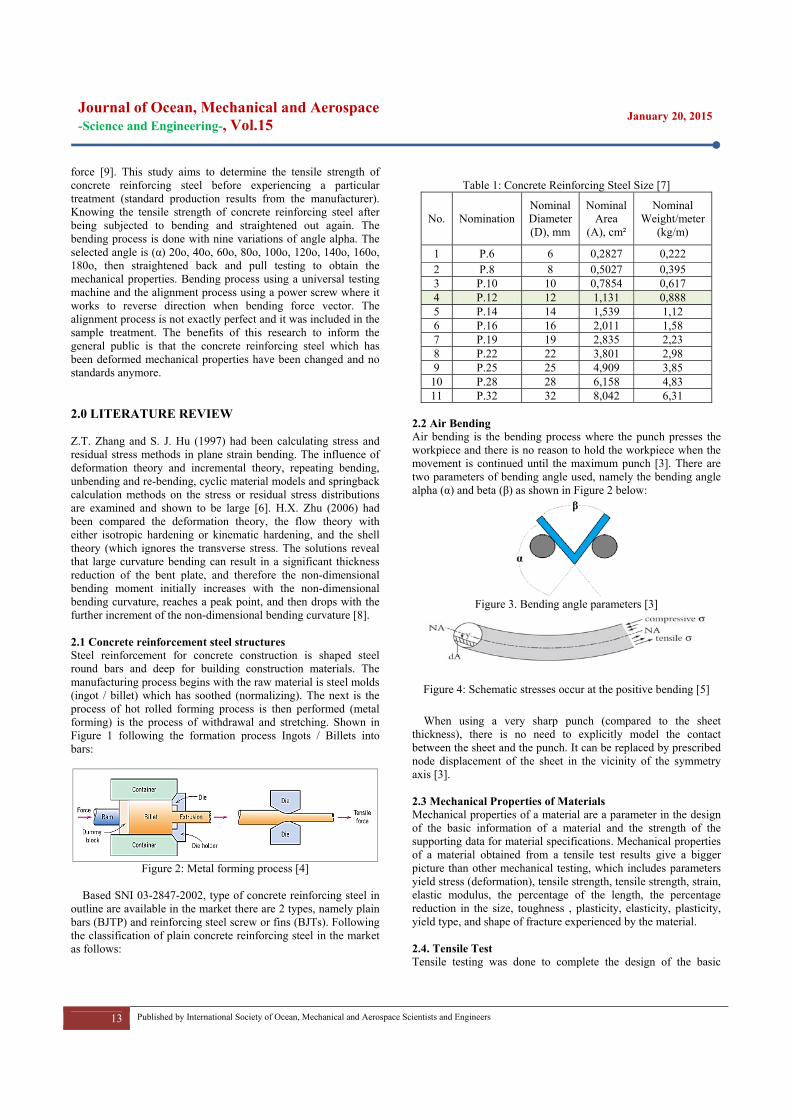
2.2 Air Bending Air bending is the bending process where the punch presses the workpiece and there is no reason to hold the workpiece when the movement is continued until the maximum punch [3]. There are two parameters of bending angle used, namely the bending angle alpha (α) and beta (β) as shown in Figure 2 below:

Figure 3. Bending angle parameters [3]

Figure 4: Schematic stresses occur at the positive bending [5]

When using a very sharp punch (compared to the sheet thickness), there is no need to explicitly model the contact between the sheet and the punch. It can be replaced by prescribed node displacement of the sheet in the vicinity of the symmetry axis [3]. 2.3 Mechanical Properties of Materials Mechanical properties of a material are a parameter in the design of the basic information of a material and the strength of the supporting data for material specifications. Mechanical properties of a material obtained from a tensile test results give a bigger picture than other mechanical testing, which includes parameters yield stress (deformation), tensile strength, tensile strength, strain, elastic modulus, the percentage of the length, the percentage reduction in the size, toughness , plasticity, elasticity, plasticity, yield type, and shape of fracture experienced by the material.

2.4. Tensile Test Tensile testing was done to complete the design of the basic


January 20, 2015


information of a material strength. In tensile testing, the specimen is loaded coaxial tensile force that grew continuously. Along with the observations made regarding the extension experienced by the test specimen.

o

FA

σ = (1)

ε =

o

LLΔ = i o

o

L LL− (2)

Dimensions of the test specimen have been determined based

on American Standard Testing and Material (ASTM) E8M that is shown in figure 5.

Figure 5: ASTM E8M [1]

The data was first generated from tensile testing machine is a drag curve. Furthermore, from these data are converted into engineering stress strain curve (using equations 1 and 2). Engineering stress strain curve result from tensile test data can be to find some sort of mechanical properties, among others:

2.4.1. Strength It is the response of a material to a force per cross-sectional area of the working force in which it is granted [4]. Mechanical properties of tensile strength are further divided into three kinds of conditions based on engineering stress strain curve [4], namely: a. Yield Strength (Yield Strength) That is occurred at the beginning of the start of plastic deformation. Method of determining the yield strength is 0.002 of distance of its strain and takes the parallel line into the curve. b. Maximum Tensile Strength That is the maximum stress that occurs (curve peaks) in the engineering stress strain curve. c. End Strength (Fracture Strength) That last stress that occurs just before the specimen broke. d. Modulus of elasticity Elasticity is the ability of a material to return to its original shape when the applied force has been removed [4]. The modulus of elasticity is the value of the stiffness of a material in which the proportional ratio between stress and strain in the elastic region in the stress-strain curve is characterized by the slope of the curve. c. Ductility (Ductility) Ductility is a term to measure how much plastic deformation occurs until the material is dropped (Fracture) [2]. In the tensile test, ductility measured in two ways:

1. Reduction of Area

% 100%o f

o

A ARA x

A−⎛ ⎞

= ⎜ ⎟⎝ ⎠

(3)

2. Elongation

% 100%f o

o

l lEL x

l−⎛ ⎞

= ⎜ ⎟⎝ ⎠

(4)

3.0 METHODOLOGY

The methodology that used is experimental. The samples of material used is concrete reinforced steel structure production from PT. Krakatau Steel (Indonesia) is known enough to have credibility in issuing a product with consistent specifications. Steel structures are widely sold in the city of Pekanbaru and used in a variety of building construction.

3.1 Grouping Sample of Testing Performed with varying bending angle, it is starting from the point (α) of 20°, 40°, 60°, 80°, 100°, 120°, 140°, 160°, 180°. The number of test specimens for each angle is not bent and bent test specimen is 5, so that for the test conditions are 45 test specimens. Total Specimens for tensile test specimens was 50. 3.2 Research Procedures

START

PROBLEM DESCRIPTION

OBJECTIVE

LITERATURE REVIEW

THEORITICAL DESCRIPTION

PREPARING MATERIAL AND EQUIPMENT

PREPARING OF SAMPLE

BENDING

STRAIGHTENINGTENSILE TEST

ANALYSIS DATA

FINISH

RESEARCH BACKGROUND

Figure 6: Flow Chart.


January 20, 2015


The first step is the process of cutting steel bars (12 mm of diameter) into 50 pieces. Once the cutting process was done, the process of turning at the central part of the specimen is to be ASTM E8M as shown in figure.7.

Figure 7: Preparing of samples

The next is making holes on each end of the specimen to the laying of the retaining pin when the tensile test. Furthermore, the bending process is carried out with nine variations of the bending angle. After the bending process, straightened out again with aligners were done. The results of the alignment are not perfect and this tends included in the sample treatment as shown in figure.8.

Figure 8: Bending and straightening

The curve resulting from tensile testing machine further

processed to determine how much the yield strength and tensile strength.

Figure 9: Tensile Test

4. RESULTS AND DISCUSSION

After a series of tensile tests on each specimen, the initial data are curves tensile testing. Tensile curve further converted into engineering stress vs. strain using eq. (1) and eq. (2). The curve is then determined the value of the yield strength and tensile strength of the maximum value. From the data in get it is seen that the yield strength and maximum strength increases with increasing magnitude of the bending angle as shown in figure.10 and figure.11. Although there are some data that appears looks random, but the increase can be seen when the data are averaged. Tensile test data as follows:

Figure 10: Yield Strength versus bending angel

Figure 11: Ultimate tensile strength versus bending angle.

Data that has been averaged subsequently collected as shown in Table 2 as follow:


January 20, 2015


Table 6: The Average of tensile strength after bent

No Bending Angle (α)

Yield Strength

(Mpa)

Ultimate Tensile strength (Mpa)

1 0 571.3418 643.0496 2 20 564.2014 669.6719 3 40 542.4107 576.5689 4 60 577.5342 615.38925 80 645.3131 678.2813 6 100 635.0545 704.0271 7 120 574.8261 629.3563 8 140 614.9339 652.4639 9 160 662.9607 699.8821

10 180 649.1896 685.2347

The value of ductility was calculated using equation 3 and 4. The value increasing of tensile strength is caused by a strain hardening which increases the strength and lower ductility [8]. Evident from the data that the extension percentage value and reduction of area decrease as the size increases the bending angle. It is shown in Figure 11 and Figure. 12 as follows:

Figure 12: Elongation versus bending angle

Figure 13: Reduction of area versus bending angle

The alteration of tensile strength at each bending angle can increase and can also decrease is shown In Table 7 as follows:

Table 7: Percentage alteration of strength. Bending

Angle Yield (%) Ultimate(%)

0 0% 0% 20 -1% 4% 40 -5% -10% 60 1% -4% 80 13% 5%

100 11% 9% 120 1% -2% 140 8% 1% 160 16% 9% 180 14% 7%

5.0 CONCLUSION

Based on tensile test data, it can be concluded that the increasing percentage of the yield strength is 14% and the tensile strength is 7% on bending angle of 180 degrees alfa. The maximum decreased elongation is 13.42% (α = 180º) from 24.67% (α = 0º) and the reduction of area is decreasing 1.93 %. For the more result of accurate data should represent the number of samples multiplied. ACKNOWLEDGEMENTS The authors would like to convey a great appreciation to Universitas Riau for supporting this research.


January 20, 2015


REFERENCES 1. Annual Books of ASTM Standards. Metals Test Methods and

Analytical Procedures. USA. Section Three, Volume 03.01. 1996.

2. Soboyejo, Wole, “Mechanical Properties of Engineered Materials”. New York: Marcel Dekker, 2002

3. D. Reche, J. Besson , T. Sturel, X. Lemoine, A.F. Gourgues-Lorenzon a. Analysis of the air-bending test using finite-element simulation Application to steel sheets. MINES Paris Tech, Centre des Mate ´riaux, CNRS UMR 7633, BP 87, 91003 Evry Cedex, France

4. William D. Callister, Jr., David G. Rethwisch, “Materials Science and Engineering”, ISBN 978-0-470-41997-7

5. Clifford, Michael, Richard Brooks, Alan Howe, Andrew Kennedy, Stewart McWilliams. 2009. An Introduction to Mechanical Engineering: Part 1. London: Hodder Education, An Hachette UK Company.

6. Z. T. Zhang, S. J. Hu. 1997. Stress and residual stress distributions in plane strain bending. Department of Mechanical Engineering and Applied Mechanics, University of Michigan, Ann Arbor, MI 48109, U.S.A.

7. SNI 03-2847-2002, SNI 07-2052-2002, Indonesian Standard of Concrete reinforcing steel structure.

8. H.X. Zhu. 2006. Large deformation pure bending of an elastic plastic power-law-hardening wide plate: Analysis and application. School of Engineering, Cardiff University, Cardiff CF24 OYF, UK

9. Arild H. Clausen, Odd S. Hopperstad, Magnus Langseth. 2001. Sensitivity of model parameters in stretch bending of aluminum extrusions. Elsevier Science Ltd: International Journal of Mechanical Sciences.


January 20, 2015


The Floating Production, Storage and Offloading Vessel Design for Oil Field Development in Harsh Marine Environment

Ezebuchi Akandu,a,*AtillaIncecik,a and Nigel Barltrop,a

a)Department of Naval Architecture, Ocean and Marine Engineering, University of Strathclyde, Glasgow, United Kingdom *Corresponding author: [email protected] Paper History Received: 3-December-2014 Received in revised form: 10-January-2015 Accepted: 19-January-2015 ABSTRACT The oil and gas exploration and production activities in deep sea are now on a steady increase globally. Therefore, it is necessary to design a cost effective and safe system for these operations. The main objective of this research is to design a Floating Production, Storage and Offloading (FPSO) vessel suitable for operation even in extreme meteorological and oceanographic conditions. In order to achieve this, the effects of extreme environmental loads on the vessel have been evaluated in terms of the maximum responses in surge, heave and pitch modes of motion. Furthermore, an interactive programme, the Principal Dimensions Programme (PD Prog) has been designed to accurately evaluate and optimise the principal particulars based on the required storage capacity and response analyses. Results show that the vessel length, which is directly proportional to the cube root of the cubic number (the overall volume), is a measure of the critical wavelength. Close to the critical wavelength in extreme metocean condition, the vessel could be subjected to several billions Newton meter of Wave Bending Moment. This design technique, in addition to the numerous useful data obtained, helps to ensure good performance during operation and so reduces downtime, and increases uptime, safety and operability of the vessel even under extrememetocean conditions. KEY WORDS: FPSO; Principal Dimensions; Extreme Environmental Loads; Responses; Wave Bending Moment. NOMENCLATURE w weight/length of cable line in water a The horizontal component of cable tension per w

Minimum separation of heave- and-pitch zeros Gamma function

Other symbols are defined in the sections where they are used. 1.0 INTRODUCTION The conceptualization and creation of floating storage vessels became imperative and feasible when the offshore oil industry began to grow in the second half of the twentieth century. The first floating storage vessels were then installed to reduce the cost of transporting oil ashore for storage before shipping it elsewhere. These first floating storage units (FSU) were tankers that stayed moored for a few days to weeks. These vessels were developed with the single point mooring system. This mooring system allows for the vessel to be positioned such that environmental impacts are minimized.

Platform operators began to look into vessels that would remain on station for periods of months to years. This type of vessel would have to be offloaded by a shuttle tanker. The logical progression was to convert mid-sized tankers into the floating, storage and offloading (FSO) vessels. These vessels however, still did not produce the oil. Thus, the oil had to be processed on a platform. Companies saw removing the platform as a way to reduce the cost of production. This led to the idea of putting production topsides on the FSO vessels. These developed into floating production, storage, and offloading (FPSO) vessels. The early FPSO vessels were tanker conversions which eventually led to drastic reduction in available fleet of tankers and so provoking the designing and building of new ones.

Generally, the needs related to the use of ship-shaped offshore units (FSU, FSO, and FPSO etc.) and their technical challenges for the development of offshore oil and gas in deep water are given by Henery and Inglis[1], Bensimon and Delvin[2] and Hollister and Spokes [3] among others.

These offshore units have proven to be reliable and cost-effective solutions for the development of offshore fields in deep waters of more than 1,000m depth, as they have successfully been applied for more than 38 years in such harsh environments.


January 20, 2015


It is note-worthy that a concrete barge with steel tanks became

the first dedicated FPSO application and it was operated by Arco in the Ardjuna field in the Java Sea offshore Indonesia in 1976 [4], while the first tanker-based single-point moored FPSO facility is the FPSO Castellon for Shell offshore Spain in 1976. Since then, the application of FPSOs and other related offshore structures has grown very rapidly, and will remain a mainstay in the oil and gas industry for many years to come as they provide the flexibility and sound economics of producing and storing at the offshore well sites. Thus the oil is produced, safely stored and then directly transported to the refinery. 1.1 The Main Objectives The purpose of this study is to design an FPSO capable of withstanding harsh metocean conditions. In other words, the research investigates the impact of harsh or extreme environmental forces on FPSO and establishes reliable methods and tools for prediction of environmental loads and structural responses. The dynamic behaviour, induced motions or responses of the vessel under the influence of these metocean forces are vital to the stability and safety of both the vessel and crew and so will be evaluated. The FPSO is to be designed for worldwide operation. To achieve this objective, the extreme metocean forces, associated extreme motion responses as well as the shear forces and bending moments for the design environment will be determined. That is, specifically, the objectives include the following:

Predict extreme vessel motion responses associated with harsh marine environmentin comparism with the benign wave (North Sea and West African).

Develop simpler methodology and programs for quick determination of design data. The design of the vessel's principal dimensions required for the development of any given oil field will be carried out based on the specified required storage capacity of the vessel.

Evaluate the dynamic wave bending moment amidships. This is required in order to ensure that the hull girder has sufficient strength to withstand the induced stress.

2.0 DESIGN METHODOLOGY The design of floating structures is usually carried out following a well-defined design spiral as a guide. This project therefore follows a simply-defined design spiral to accomplish the desired goal(s). The FPSO Design Spiral (FDS) usually starts with the identification of the vessel owner's requirements. The elements of the spiral include, but not restricted to the following steps: (i) Owner's Requirements, (ii) Environments, (iii) Hydrostatics, (iv) Motions, and (v) Structure. In order to meet the owner's requirements such as the required storage capacity, it is important to ensure that the right principal dimensions of the vessel are evaluated as demonstrated in the following sections.

Generally, the following preliminary design objectives are adopted for optimal design of vessels which are to be operated the harsh wave environment such as the North Sea: (i) The storage capacity or volume must be capable of taking the output during the average interval of shuttle tanker calls plus about 3 days. (ii) The value of the transverse metacentric height, , must be around 3 or more, in the fully-loaded condition. (iii) The natural rolling period must be greater than 12 seconds. Also, the natural pitching and heaving periodsmust be as long as possible. Usually, a good design usually has the natural motion periods longer than the peak period of the spectrum which is exceeded for less than 2% of the time and low heave forces and pitch moments at all shorter periods. Table 1 gives the wave periods and wavelengths for four sea areas which illustrate the problems involved. For instance, the peak periods exceeded 2% of the time in the Central and Northern North Seas are 12.3s and 15.4s respectively. (iv) In order to ensure a better motion response, the zero force frequencies for heave and pitch must be spread out as much as possible. (v) The ratio / must be less than 13 (from structural point of view). (vi) In order to accommodate the segregated ballast and the produced water storage capacity, the under deck volume should not exceed 1.8 times the displacement. This implies that:

/ 1.8 . (vii) The required external surface areas should be as small as possible, which implies low / and / ratios. (viii) The induced motions should not exceed the levelswithin which the separators have been designed to operate. Conventional separators have been designed to cope with the following levels of motion: Angular motions, 0 to 7.5o; linear motions, 0 to 0.25g; periods, 3 to 15s [5]. Table 1: Wave Periods and Wavelengths for a Number of Sea Areas

Periods and Wavelengths Exceeded 2% of Time

Pierson-Moskowitz JONSWAP

Area Tz Tp [s] [m] Tp [s] [m]

Central North Sea 8.7 12.3 236 11.2 196

Northern North Sea 10.9 15.4 370 14.1 310

West of Shetland 11.3 15.9 395 14.6 333

Brazil 10 14.1 324 12.9 260

Spectral Analyses are carried out for each of the vessels with above preliminary objectives being applied as design constraints in the computer programmes written in MATLAB. The PD Programme and the WavBem have been carefully written to evaluate the optimal principal dimensions and the wave bending moment distribution using the required storage and efficiency as major inputs to the programmes. 2.1 Owner's Design Requirements Vessels are often designed to perform specific function(s). The FPSOs are used mainly for production and storage of crude oil (and periodically offloaded to shuttle tankers for transportation to


January 20, 2015


the refinery or market). Therefore, most vessel owners require reasonably high storage capacity and large deck area for topside installation.

Major oil fields in the Niger Delta area of Nigeria have oil reserves up to 1000 million bbls of oil. Agbami, Bonga, Forcados-Yokri, and Erha fields have oil reserves of 1000, 600, 1235, and 1200 million bbls respectively [6]. See Table 2.

Therefore, most vessel owners would require FPSOs that would be capable of storing up to 2 million bbls. Agbami FPSO has storage capacity of 2.2 million bbls. It is therefore important to have a reasonably sufficient specific storage capacity in mind as an initial design requirement. In this paper, we will be considering a storage capacity of 2 million bbls and will also be assuming that this vessel is meant for unrestricted service location. It is therefore imperative to consider in the design stage, the effects of extreme environments in which its services may be required.

Table 2: Major Oil Reserves in the Niger Delta of Nigeria

Operator Fields Reserves (mmbbls)

Shell Bonga 600

Forcados-Yokri 1235

Nembe Creek 950

Mobil Erha 1200

Ubit 945

Chevron Texaco Agbami 1000

Meren 1100 2.2 The Wave Environment There are several challenging wave environments in which oil and gas exploration activities still take place. The North Sea of the United Kingdom is a very good example of such. Any offshore floating structure designed for this region can be redeployed to other locations for operation since most adverse effects of very rough, irregular and phenomenally high wave conditions might have been accounted for.

In offshore structural design, it is convenient to describe the wave environment in spectral form. The general form of the wave spectrum model is given by:

The parameters (A, B) of the Spectrum are solved in terms of the significant wave height and the wave period (which are in common use in wave description) for specified values of p and q (For Pierson-Moskowitz spectrum, p=5 and q=4). The nth moment of the spectrum which is very useful in obtaining the wave characteristics is expressed as:

1 // 1

The zeroth moment (n=0, mn=m0) or the variance of the wave

elevation is defined as the area under the Spectral curve. The mean wave frequency is the ratio of the first moment to the zeroth moment. The zero-crossing frequency is the square root of the ratio of the second moment to the zeroth moment. The

spectral peak frequency can be obtained by differentiating with respect to the wave frequency, and equating the result to zero.By substituting the expressions for A and B, the modified version of the wave spectrum is therefore obtained as:

124 exp 496.1 2

The rectangular-shaped floating production, storage and

offloading vessel with length L, Beam B and draught T, (which are evaluated based on the required storage capacity as given in eqns. 1-5) is be operated in the North Sea of 100-year Return Period storm; the zero up-crossing period and significant wave height are 17.5s and 16.5m respectively. The equation of motion of this vessel is given by:

3

Where: Mjk are the elements of the generalized mass matrix for the structure; Ajk are the elements of the added mass matrix; djk are the elements of the linear damping matrix; Cjk are the elements of the stiffness matrix; Fjare the amplitudes of the wave exciting forces and moments, j and k indicate the directions of fluid forces and the modes of motions; represents responses;

and are the velocity and acceleration terms; and is the angular frequency of encounter. 2.3 Hydrostatics The elements of the stiffness matrix or the hydrostatic restoring force coefficients, Cjk, are important in the station-keeping of the vessel and therefore must be carefully evaluated. In surge mode, it can be shown that the uncoupled restoring coefficient, which is largely contributed by the mooring lines, may be given by:

1 2 12

4

The stiffness or coefficients of restoring force and moment in

heave and pitch motions can be estimated as functions of the buoyancy due to a unit length of sinkage respectively.

5

12 12 6

2.4 The Principal Dimensions of FPSO There are three major factors that greatly influence the size and arrangements of these different parts of the Floating Production, Storage and Offloading system and its process plants. These are: (i) Provision of sufficient oil storage capacity, (ii) Provision of enough topside area or space for process plants, accommodation, helideck and other required topside equipment and (iii) Provision of displacement and ballast capacity. These factors are directly related to (or functions of) cubic number, length-breadth ( ) and breath-depth ( ) ratios (as variables in the analysis) respectively. The cubic number is the overall volume of the vessel and it is directly proportional to the required storage capacity. With the


January 20, 2015


knowledge of the oil storage efficiency, the cubic number and the preliminary evaluation of the principal dimensions can made. The overall volume or the cubic number is given by:

LBD /

D

D⁄ 7

From eqn. (1), it follows that:

The Length, L/

8

Breadth, B/

9

Depth, D/

10

Draught, T D 11

is the displacement; and the new dimensionless factors are: / ; ⁄ / ; / , : Required

oil storage capacity in barrel (bbl); : Oil Storage Efficiency; and Conversion factor, 6.28981077; 6.289810771 . 3.0 WAVE LOADS AND RESPONSES 3.1 Surge Force and Response In surge mode of motion, the acceleration or added mass force is out of phase with the Froude-Krilov Force. It will be wrong to add them up algebraically. Since the added mass force is very small compared to the Froude-Krilov force especially within the relevant frequency range, the surge excitation force amplitude, F1, is usually taken to be approximately equal to the amplitude of the Froude-Krilov (pressure force), as given in Eq. (12).

ζ 2B

k 1 e T sin 2

ζBλπ 1 e T/ sin

πλ

12

Therefore, the Surge Response Amplitude Operator, RAO1, is:

ζ2 B

k 1 e T sin 2 13

Q1 is the surge dynamic amplification factor. 3.2 Heave Force and Response Assuming the vessel has a constant mass density, zero forward speed and moored in deep sea, with a sinusoidal wave

propagating along the negative x-axis (head sea), the velocity potential is:

cos 14 The vessel is divided into strips of equal sizes and the force acting on each strip ( ) is the sum of the pressure force and the added mass force. These forces are integrated across the length of the vessel to obtain the expression for the heave excitation force.

sin

sin

2 sin 2 sin Where is the 2-D added mass in heave, while the amplitude of the heave force is given by:

2ζ g e T2

ζBλπ 2 e T sin

k2 15

Therefore, the Heave Response Amplitude Operator, RAO3,

defined as the heave amplitude per wave amplitude, is:

ζBλπ 2

e T sink2

… 16

: Dynamic magnification factor in heave; λ: wavelength; : virtual added mass coefficient in heave; ζ : wave amplitude; and wave number, k 2 λ⁄ . Both heave force, and response, will be equal to zero

when B or is equal to zero. These happen

at wavelengths of , L, L/2, L/3 etc. 3.3 Pitching Moment and Response The amplitude of the pitching moment has also been obtained following similar procedure and it is given by:

ζBλπ 2

e T

2 cos 2 2

… 17 So, the Pitch Response Amplitude Operator, RAO5, defined as the pitch response amplitude per wave amplitude, is:

ζ


January 20, 2015


Bλπ 2

12 cos 2 2 18

is the dynamic magnification factor in pitch motion.

The pitch moment, and its corresponding response, will

be equal to zero if B or cos is

equal to zero. These happen at wavelengths of , L/1.43, L/2.45, L/3.47, L/4.49 etc. To ensure that the vessel has a very good motion performance, these wavelengths must be well-separated from one another.

Investigations show that the minimum separation of heave- and-pitch zeros is given by:

4,

1.43 4 19

The overall induced kinetic energy due to wave impact is the

sum of the energies in thecorresponding modes of modes of motions. For heave and pitch modes of motion, this energy depends on the values of energy coefficients, , at various wavelengths.

20

The wavelengths at which these energy coefficients, , tend to

infinity are called critical wavelengths, λ .It is important to note that these phenomena occur at heave zeros. That is, L/λ , where 1,2,3, … 4.0 DYNAMIC WAVE BENDING MOMENT 4.1 Wave Induced Shear Force The Shear Force at any point from the one end is the integral sum of the contributions from wave excitation force, restoring force and inertia force and damping force. The Shear Force, from one end of the vessel is therefore given by: On the elemental strip:

sin

4.2 Wave Bending Moment The vertical dynamic bending moment at any point from the one end is the integral sum of the contributions from wave excitation load, restoring load, and inertia moment load and damping load.

cos sin cos1 sin cos sin

12

23

23

23

21 Let sin cos

1 sin cos

2

3

2

22

cos sin

3

2

3

23

Where the damping factor is:

The amplitude of the bending moment distribution per unit

wave amplitude is expressed as:

/ 24

5.0 RESULTS AND DISCUSSIONS From the design 1 (see Table 3) analyses (which are executed in the PD programme with other subroutines and theoretically described in this paper), the most probable maximum amplitudes of surge, heave and pitch motions are 13.4m, 11.3m and 7.1o respectively. The linear motions have a maximum acceleration of 0.9m/s2 or 0.09g. These are all within the acceptable levels of motion within which the conventional separators can cope.

However, this vessel could experience wave bending moment up to 10 billion Newton meter in this design harsh wave condition. All the preliminary design objectives were achieved


January 20, 2015


except that the minimum separation of heave and pitch zeros is small (about 10m). Table 3: Analysis of Rectangular Block Design for Oil Storage Capacity of 2 million barrels

Design 1: ( : 10

L B T L/B B/D B/T 306.

4 56.7 22.1 5.4 1.8 2.57 1.46

Heave and

Pitch Zeros

Heave Zeros Pitch Zeros

4 L

L2

L3

L1.43

L2.45

L3.47

204.5 306.4 153 102 214 125 88.3

Metacentric Heights and Natural Periods

, λ

355 371 14.8 343 6.43 23.2 17.2

Required Oil Storage Capacity and Vessel Size

Sc [Mbll

]

Es [%] M [t] m Hull

Area TopAre

a TransAre

a

2 58 393356 383762 57679 17390 1789

Figure 1: The Bending Moment per unit wave amplitude at various sections of the vessel from aft to amidships Table 4: Comparism of predicted Wave Bending Moments [inMNm] with those of ABS and DNV (Vessel: Design 1)

BM (Predicted) BM (ABS) BM (DNV)

Sagging 10105 10701 10256

Hogging 10812 10872 11282

Design 2 (See Table 5) shows a vessel of equivalent storage capacity as that of design 1 but with an improved minimum separation of heave and pitch zeros. Consequently, the dynamic performance is equally improved. This improvement is also notable in the reduction of the design wave bending moment at amidships as shown in Table 6.

Table 5: Design 2 showing improvement in Design 2: ( : 23

L B T L/B B/D B/T

256.9 54.7 25.4 4.7 1.4 2.2 1.5 Table 6: Comparism of predicted Wave Bending Moments [in MNm] with those of ABS and DNV (Vessel: Design 2)

BM (Predicted) BM (ABS) BM (DNV)

Sagging 9329 7066 7040

Hogging 9982 7180 7743 5.0 CONCLUSIONS

A series of formulae have been given and systematically programmed for the determination of an optimal set of principal dimensions to meet a specified field output in a given harsh environment (the North Sea conditions were chosen).

The extreme responses in surge, heave and pitch motions have been evaluated and these are all within the acceptable levels of motion required for the smooth operation of the oil separators. Therefore, operational downtimes are minimized.

The critical wavelengths have been found to be prime factors of the vessel length (which is directly related to the cubic number).

There should be sufficient separation of heave and pitch zeros as this is necessary to improve the performance of the vessel. Larger separation of heave and pitch zeros also leads to the reduction in the induced wave bending moment acting on the vessel. ACKNOWLEDGEMENTS The work reported here has been supported by the Federal Government of Nigeria through the Petroleum Technology Development Fund. The authors are grateful for this support. REFERENCE 1. Henery, D., and Inglis, R. B. (1995). "Prospects and

challenges for the FPSO." Offshore Technology Conference, OTC 7695, Houston, May.


January 20, 2015


2. Bensimon, L. F., and Delvin, P. V. (2001). "Technology gaps and preferred architectures for deepwater FPSOs." Offshore Technology Conference, OTC 13088, Houston, May.

3. Hollister, H. D., and Spoke, J. J. (2004). "The Agbami project: A world class deepwater development." Offshore Technology Conference, OTC 16987, Houston, May

4. D'Souza, R., Delepine, Y., and Cordy, A. "An Approach to the Design and Selection of a Cost-effective Floating Production Storage and Offloading System." Proc., Offshore Technology Conference.

5. Miller, N. S. (1992). "Review of Reasons for Selecting a Floating Production System." Advanced Design for Ships and Offshore Floating Systems.

6. Adebola, D. F., Okoro, J., and Nwasike, O. (2006). "Building local capability: a case study of Agbami project." A paper presented at the 30th SPE Annual International Conference and Exhibition (NAICE 2006), Abuja, Nigeria 31st July–2nd August.

Publishe

ed & Printed

ISOReJalPekhtt

d OMAse esty Menara Hlan Sisingamakanbaru-Riautp://www.isom

Hotel angaraja No.89u, Indonesia mase.org/

9

Teknik MFakultasUniversIndoneshttp://ft.

Mesin s Teknik itas Riau, ia .unri.ac.id/

IISSN: 2354-70065

Documents

Vol.15, January.2015 ISSN 2354-7065 - isomase.orgisomase.org/JOMAse/Vol.15 Jan 2015/Vol-15.pdf · Buana Ma’ruf (Badan Pengkajian dan Penerapan Teknologi, Indonesia) ... The equation