Visualizing a Flutter Mechanism as a Traveling Wave Through

American Institute of Aeronautics and Astronautics

1

Visualizing a Flutter Mechanism as a Traveling Wave Through Animation of Simulation Results for the

Semi-Span Super-Sonic Transport Wind-Tunnel Model

David M. Christhilf * Analytical Mechanics Associates, Inc., Hampton, VA, 23666

It has long been recognized that frequency and phasing of structural modes in the presence of airflow play a fundamental role in the occurrence of flutter. Animation of simulation results for the long, slender Semi-Span Super-Sonic Transport (S4T) wind-tunnel model demonstrates that, for the case of mass-ballasted nacelles, the flutter mode can be described as a traveling wave propagating downstream. Such a characterization provides certain insights, such as (1) describing the means by which energy is transferred from the airflow to the structure, (2) identifying airspeed as an upper limit for speed of wave propagation, (3) providing an interpretation for a companion mode that coalesces in frequency with the flutter mode but becomes very well damped, (4) providing an explanation for bursts of response to uniform turbulence, and (5) providing an explanation for loss of low frequency (lead) phase margin with increases in dynamic pressure (at constant Mach number) for feedback systems that use sensors located upstream from active control surfaces. Results from simulation animation, simplified modeling, and wind-tunnel testing are presented for comparison. The simulation animation was generated using double time-integration in Simulink of vertical accelerometer signals distributed over wing and fuselage, along with time histories for actuated control surfaces. Crossing points for a zero-elevation reference plane were tracked along a network of lines connecting the accelerometer locations. Accelerometer signals were used in preference to modal displacement state variables in anticipation that the technique could be used to animate motion of the actual wind-tunnel model using data acquired during testing. Double integration of wind-tunnel accelerometer signals introduced severe drift even with removal of both position and rate biases such that the technique does not currently work. Using wind-tunnel data to drive a Kalman filter based upon fitting coefficients to analytical mode shapes might provide a better means to animate the wind tunnel data.

Nomenclature

M = Mach number q = dynamic pressure TDT = Transonic Dynamics Tunnel HSR = High Speed Research S4T = Semi-Span Super-Sonic Transport RCV = All-moving Ride Control Vane FLAP = Wing trailing edge control surface (flap/aileron) HT = All-moving Horizontal Tail LTI = Linear Time Invariant SAREC-ASV = Simulation Architecture for Evaluating Controls for Aerospace Vehicles

* Engineer-4, TEAMS-2 Contract, c/o NASA-LaRC, Mail Stop 308, AIAA Senior Member.

https://ntrs.nasa.gov/search.jsp?R=20140011910 2018-04-06T04:48:51+00:00Z


2

I. Introduction ISUALIZATION of modes of vibration has been around for a long time in terms of still shots of vibration mode shapes. Animation of simulation results by means of superposition of mode shapes of different

frequencies and varying amplitudes are currently in general use,1,2 some including visualization of a flow field.3 A common aspect is that, since the dynamics are computed analytically, the deformations are known from the modeling. There has also been development of techniques for taking test data and deriving time histories of structural deformations for use in animations. That can take the form of optically tracking markers placed on an airframe,4 in a manner similar to motion capture techniques used by the movie industry to generation animations based on the movements of actors.5 One particularly useful technique is to use onboard accelerometers to synthesize displacements at selected points, and fitting amplitudes for assumed (modal) shape functions in order to have estimated displacements available on a much finer grid, while receiving and processing the signals as telemetry data in near-real time.6

For the S4T aeroservoelastic wind-tunnel model, both simulation and wind-tunnel data were available from previous development and testing of active controls systems for various purposes such as Gust Load Alleviation (GLA), Ride Quality Enhancement (RQE), and Flutter Suppression (FS).7 It was of interest to animate the motion of the wind-tunnel model using an available desktop tool, namely MATLAB with handle graphics. The simplest approach that seemed likely to work for both simulation and wind-tunnel data was to take accelerometer time histories and apply two time integrations to get estimates of displacements at accelerometer locations, while connecting the accelerometers with a network of line segments.

The technique did not work well for the wind-tunnel data. The calculated displacements for the wind-tunnel data tended to drift to large values in an unorganized spatial distribution that did not give meaningful insight into the deformation of the actual airframe. This effect persisted even when the means were subtracted from the signals for each one-second interval prior to integration. Frequency filtering, and subtracting the means from the rate signals prior to the second time integration may serve to improve the results, but so far the results for display of wind-tunnel data have not been useful. However for the simulation data, the animation technique worked surprisingly well. Specifically, for the S4T wind-tunnel model in the test configuration with ballast added to the two engine nacelles,8 the animation indicated that fully developed flutter takes the form of a traveling wave, propagating from nose to tail and fully involving the fuselage as well as the wing.

Formal analytical study of the interaction of fluid flow and wave propagation dates back at least to the 19th century with investigations by Kelvin into the role wind plays in generation of water waves,9,10 and with studies by Rayleigh concerning fluttering flags and sails.11 After World War II, both analytical12 and experimental13 studies of panel flutter as related to aircraft recognized that wave propagation was clearly involved in the process of panel instability in flight. Some insights from that work seem to have been lost in textbook treatment of flutter14,15,16 that places more emphasis on computational rather than conceptual aspects.

When the source of a traveling wave is internal to a structure, the wave can be used as a means of propulsion. Apneseth, et al.17 (2010) cite references for the study of fish propulsion dating back to the 1920's and 1930's. Although most fish use body and tail for propulsion, with body length varying from a quarter wavelength (e.g. tuna) to several wavelengths (e.g. eel), the knifefish uses a ventral ribbon fin that runs for a substantial length along its body to generate a rippling wave for propulsion. The knifefish can travel forward or in reverse, depending upon the direction of the wave, and for hovering actually initiates two traveling waves that originate at each end in meet in the middle.18

Because of fluid slippage, the speed of a traveling wave in a fish must be faster than the rate of propulsion that is generated. In contrast, the rate of progress for a snake traversing through grass would equal the rate of wave propagation, due to the solid nature of the medium traversed. For water waves, flags and sails, the speed of wave propagation is necessarily slower than that of the driving relative wind, again due to fluid slippage. For the case of aircraft flutter as a traveling wave, as the dynamic pressure of the fluid medium increases, the speed of the traveling wave should tend toward, but not exceed, the speed of the relative fluid flow. Only for the case of no slippage would the speed of wave propagation equal that of the medium driving the wave.

Viewing flutter as a traveling wave has several implications for interpreting wind-tunnel observations, and for control law design for active controls flutter suppression. The purpose of this paper is to present a simple desktop animation technique, describe insights gained from that animation, and discuss implications of those insights in terms of active controls flutter suppression.

V


3

II. S4T Wind-Tunnel Model Description The S4T represents a supersonic transport concept that was the subject of study through the High Speed Research

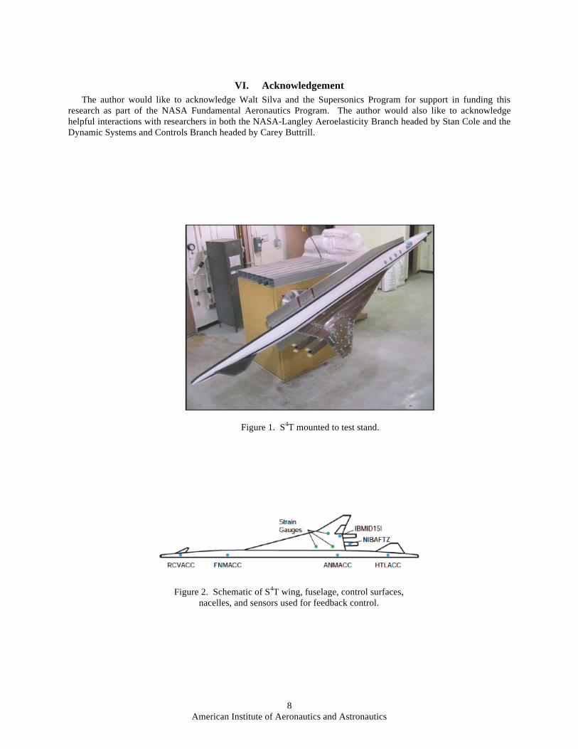
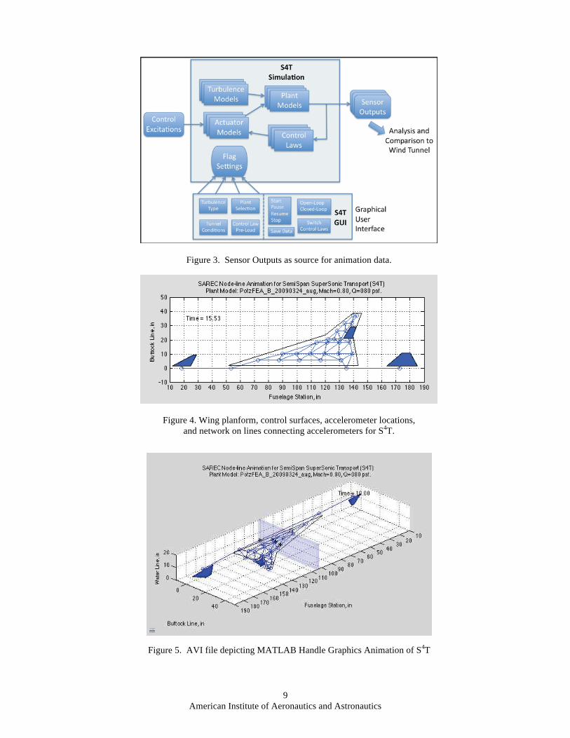
(HSR) program in the 1990s.19 The wind-tunnel model is an aeroelastically-scaled half-span model with multiple sensors and three actuated control surfaces (Fig 1).20 The wing, forward Ride Control Vane (RCV), and aft Horizontal Tail (HT) are attached to a flexible composite beam tailored to represent the fuselage stiffness properties (Fig. 2). Attached to the trailing edge of the wing is a fast-acting, bidirectional flap/aileron (FLAP) control surface. The fuselage beam is contained in a non-metric aerodynamic fairing, and the wing, RCV, and HT are attached to the fuselage beam through small gaps in the fairing. Mounted to the lower surface of the wing are two flow-through engine nacelles. The nacelles can be configured with circumferentially-mounted ballast weights in order to lower the flutter dynamic pressure to within the operating range of the NASA-Langley Transonic Dynamics Tunnel8 (TDT), and to provide a less explosive onset of flutter as compared to the non-ballasted configuration.

Linear models were generated for representing the dynamic aeroservoelastic characteristics of the wind-tunnel model.21 These linear models were packed into a MATLAB Linear Time Invariant (LTI) Object, and incorporated into a Simulink simulation based on the Simulation Architecture for Evaluating Controls for Aerospace Vehicles (SAREC-ASV) simulation architecture (Fig. 3).22 The simulation was used as one means for evaluating feedback control laws prior to closed-loop testing during two entries in the TDT during 2009 and 2010. Results of those tests were reported in reference 7. The simulation animation was developed subsequent to the most recent wind tunnel testing.

III. Animation Implementation In an effort to gain insight into the flutter mechanism for the S4T and the interaction between active controls and

vehicle flexure, a means was sought for computing and displaying structural deformations and control surface deflections as functions of time. The method chosen was to take accelerations calculated with the SAREC-ASV simulation at each sensor location and apply two time integrations in order to calculate displacements. The simulation accelerometer signals had known biases added to represent gravity and any instrumentation offsets. Those known biases were subtracted prior to the first integration. Potentially a bias could have been determined and subtracted before the second time integration, but that was not found to be necessary. The integrations were implemented within the Simulink simulation itself, and the displacements were provided as additional outputs (Fig. 3). The displacement time histories were then used to drive the animation.

A. Wing and Fuselage Geometry Representation

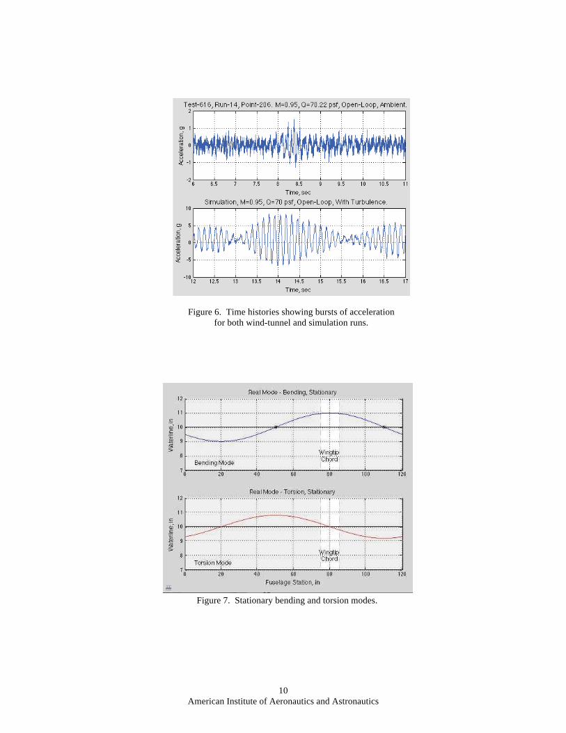
An available state space model for the S4T ('FEA'-based, Refs. 7, 21) had 28 vertical accelerometers modeled, 4 on the fuselage and 24 on the wing, corresponding to accelerometers available on the wind-tunnel model. The linear models were available for discrete values of Mach number (M) and dynamic pressure ( q ), including models that represent conditions above the open-loop flutter boundary. For animating the structural deformations, the longitudinal and lateral geometric locations for the accelerometers were plotted, with an assumed common elevation of 10 inches (waterline convention, vertical up). A network of line segments connecting the accelerometers was defined in order to give some perspective to time-varying vertical displacements at the accelerometer locations. The network defines triangles for connecting wing accelerometers, but the 4 fuselage accelerometers were connected by line segments aligned fore and aft, with only the center two connected to the wing (Fig. 4). The accelerometers and connecting line segments (shown in blue) were plotted using MATLAB handle graphics so that the location data for each handle-graphics object could be updated as functions of time without deleting and redrawing the objects with each time step. A stationary outline of the wing was drawn in black, at the 10 inch waterline level, for reference. Figure 5 shows a perspective view of the animation.

A key aspect of the animation is that, for each line segment that crosses through the 10 inch waterline reference plane, the location of the crossing along the length of the line segment is calculated by interpolation, and a black '*' marker is plotted there. The locations of the markers change with time as the airframe flexes. For a stationary, real-valued mode, in the absence of other modes, these markers would be stationary, indicating a node line pattern for the particular mode shape. For the more general case, with complex-valued modes that do not have fixed node lines, the motion of the markers indicates the motion of the structural deformations in a more compelling manner than merely displacing the accelerometer locations vertically.


4

B. Control Surface Geometric Representation

The S4T has three hydraulically-actuated control surfaces. The all-moving RCV is attached to the fuselage beam at what would be the pilot station for a full-sized civil transport. It is the only one of the three control surfaces that was added specifically for structural mode control. Its purpose was to provide active-controls Ride-Quality Enhancement (RQE) for the pilot, in part to improve pilotability. The all-moving HT is located on the fuselage aft of the wing. The HT is substantially larger than the RCV, and is the primary pitch control device. For animation, each of these control surfaces was represented as pivoting on a lateral horizontal shaft that translates vertically with the motion of the fuselage at the co-located accelerometer location. The control surfaces were represented using MATLAB hgtransform objects, that have an associated 4x4 handle-graphics matrix that has a direction cosine matrix that defines changes in orientation for the object as the top-left 3x3 matrix, and coordinates for a reference point on the object as the top 3 elements of the right-hand column. The data for the hgtransform matrices for the RCV and HT were updated for the vertical locations of the rotating shafts and for the pitch orientation of each control surface. For simulation data, the rotation of each control surface was defined by the output of 3rd-order position- and rate-limited actuator models, in response to commanded deflections. The commands were the sum of whatever excitation and feedback was present during the simulation. For both simulation and wind-tunnel data, a refinement to the animation would be to estimate the slopes of the fuselage at the control surface attachment points, and to apply those as corrections to the rotations for display of the control surfaces.

Animation of the FLAP control surface was more complicated. Two accelerometers located near and parallel to the hinge line for the FLAP, as well as a third location forward of the hinge line and defined as the average of two accelerometers closer to the leading edge, were used to define a plane that deflected along with the wing. The three points that define the plane were allowed to translate vertically, so that distances between the three points were not strictly constant. The hinge line itself was modeled as translating vertically to a location located in the plane defined by the three points embedded in the wing. A reference angle around the hinge line was defined by the slope of the defining plane, perpendicular to the hinge line. Deflections of the FLAP were then defined relative to that time-varying reference slope. The FLAP translation, hinge line slope, hinge line reference tilt, and control surface deflection were computed, and applied to the hgtransform object my means of its hgtransform matrix. The end result was considered satisfactory for merging the deflection of the FLAP with the flexing of the wing to which the FLAP was attached. The sign conventions for control surface deflections for all three control surfaces, as well as for displacement of fuselage and wing accelerometers, were verified by using step commands for the control surfaces, running the simulation, and animating the result to observe the steady-state response. For the wind-tunnel model and for the simulation, the sign convention for the fuselage is positive up, and for the wing and nacelles is positive down. The sign convention for the animation is: fuselage station positive aft, buttock line positive starboard, and water line positive up. The sign convention for all control surfaces is that positive indicates trailing edge down.

C. Fluid Flow Representation

Once it was observed that the flutter mode for the S4T appeared to have the character of a traveling wave, the rate of wave propagation relative to the speed of the fluid medium was considered to be of interest. In order to give some visual sense in the animation of the speed of the flow, a thin transparent blue slab, perpendicular to the flow, was drawn. The blue slab was then transported downstream at a speed determined by the Mach number and by the speed of sound for the heavy-gas medium used for testing in the TDT. When the slab reached the downstream limit of the animation, it was relocated to the upstream end in order to continue the effect.

IV. Results Once the animation of the simulation results was accomplished, it became apparent that the form of the flutter

mode for the S4T ballasted configuration was a traveling wave that traverses from nose to tail. Below the flutter dynamic pressure, the reference-plane-crossing markers tend to dance around in an unorganized fashion. For conditions above the flutter boundary (open- or closed-loop), the flutter mode is characterized by the markers generally aligning laterally and traversing from nose to tail in a distinct pattern. The speed of traverse of the markers and the distance between the marker groups define both the speed of a traveling wave and its half wavelength.

When fully developed, the ballasted S4T porpoises up and down, leading with the forward end of the vehicle with an amplitude that dominates other modes. The speed of the traveling wave was slower than the speed of the fluid flow, as judged by comparing the speed of traverse of the markers with the speed of the vertical slab that indicated the flow speed. The ballasted engine nacelles were found to accentuate the deflection of the trailing edge


5

of the wing, with phasing such that the nacelle motion was consistent with the traveling wave motion of the rest of the vehicle. Part of the explanation for the participation of the fuselage in the flutter mode likely has to do with the presence of both the RCV and the HT attached to the fuselage.

For the S4T in the non-ballasted configuration, the form of the flutter mode is different. For that case, the nose and the wing tip are in phase with each other, with the nacelles out of phase and the tail lagging behind the nacelles. If there is a general flow associated with the non-ballasted flutter mode, it would be from the wing tip to the horizontal tail, with some participation of the RCV synchronized with the wing tip. The ballast for the S4T was designed to achieve two objectives: first to bring the dynamic pressure at which flutter occurs down into a range suitable for testing active flutter suppression within the operating envelope of the TDT, and second to reduce the severity of flutter onset when crossing the flutter boundary. Simulation of the two configurations tends to confirm that the two objectives were achieved. Animation of the two configurations gives insight into what each flutter mode looks like, and for the ballasted configuration, suggests how the flutter mode is able to extract energy from the fluid flow and go unstable.

A. Simple Model for Bursts of Response

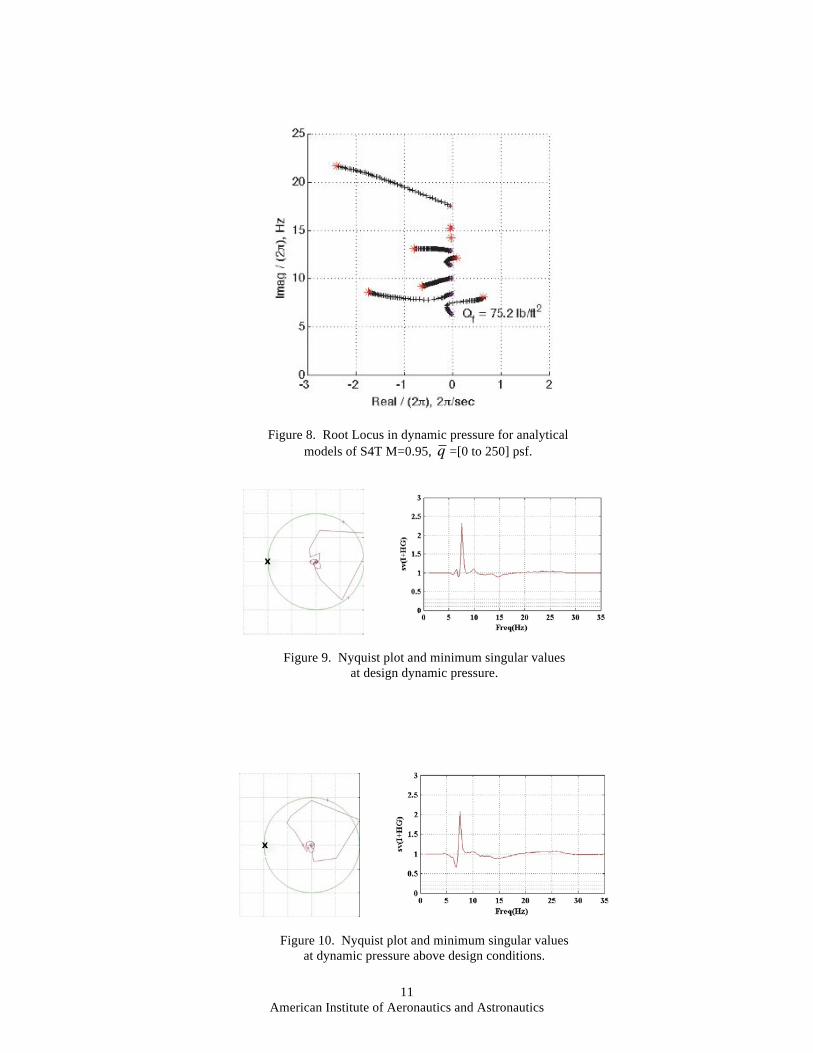
A standard method for probing the flutter boundary for the S4T was to pump heavy gas out of the tunnel to achieve low density, set fan speed to achieve a desired Mach number, and then increase dynamic pressure slowly by bleeding in more gas while adjusting fan speed in order to maintain the desired Mach number. Maintaining constant Mach number is considered important so as to not change the character of the flow. At times while operating at a dynamic pressure below the critical flutter dynamic pressure, the wind-tunnel model would exhibit bursts of vibration response that would damp out, only to be followed by additional transient bursts of response (Fig. 6). All the while the wind tunnel model would also be responding in a more random fashion across a broad range of frequencies.

The bursts of vibration gave the appearance of being a lightly damped response near the flutter frequency due to random bursts of turbulence in that frequency range. Since the flutter mode was lightly damped it would be expected to respond to excitation, but also to damp out in the absence of sustained excitation at the flutter frequency. A surprising result from simulation was to find that the simulation model also exhibited an even more pronounced tendency for bursts of response, to what was uniform turbulence, with a fairly well sustained beat pattern for certain dynamic pressures that were somewhat below the flutter dynamic pressure (Fig. 6). The simulation seems to give an indication that the intermittent transient responses were part of the character of the wind-tunnel model itself, rather than due to irregularities in the test environment.

Beating can occur in a lightly damped system that has sustained excitation at a frequency near, but not identical to, the frequency of a lightly damped mode.23 The rising and falling amplitude is due to the relative phasing between the excitation and the response. For a certain portion of time, the excitation reinforces the oscillating response, and then as the phase shifts due to the frequency difference, the excitation tends to cancel the response. Beating due to sustained excitation at a frequency close to the flutter frequency would not be expected to occur in the simulation or in the wind tunnel due to the random nature of the turbulence.

Another source of beating would be two sustained oscillations at nearly, although not quite the same frequency, but of comparable magnitudes. As with the case of sustained excitation, the two vibrations would tend to alternately reinforce and then cancel each other as the phase difference between the two oscillations changed due to the slight difference in frequencies. That also would seem to be unlikely in this case, because although classic flutter will be the result of two distinct modes with close separation in frequency interacting with each other in the presence of an air flow, the companion mode to the flutter tends to become very well damped and would be expected to be of insufficient amplitude to cause the overall response to beat.

Recognizing flutter (in the case of the S4T in the ballasted configuration) as a traveling wave provides a simple explanation for what would otherwise be a rather puzzling observation, as follows. With no airflow ( q =0), structural modes are generally modeled first as real modes with no damping, and then as real modes with artificial 'modal damping' added. Each mode has a distinct frequency. Real modes are stationary by their nature, with fixed node lines (or fixed node points for a 2-dimensional representation, Fig. 7). The non-shaded portion of Figure 7 indicates what a stationary mode might look like for a spanwise view of an unswept, high aspect ratio wing. When two real modes are close in frequency, they can combine in effect to form traveling waves. The directionality of the traveling wave depends upon the relative phasing between the two real modes. Since the two real modes are close to, but not exactly, the same frequency, the relative phasing will change with time, such that for a portion of time the two real modes will interact as a traveling wave going downstream. Such downstream motion will be capable of extraction of energy from the fluid flow, which can lead to instability. However, since the frequencies are not the


6

same, the phasing will change such that the two modes will act as a stationary wave, and then as a wave that travels upstream. During the time that the two real modes interact to form a wave traveling upstream, the motion will be opposed by the fluid flow, and the vibration will be well damped. So the bursts of response to uniform turbulence may be explained as two real modes of nearly the same frequency that alternate between the character of a traveling wave going downstream, and one going upstream.

Although the example can be shown to work for strictly real modes, in practice that is not actually the case. Once unsteady aerodynamic terms are added to a structural model (i.e. q >0), all the modes become complex, although for low dynamic pressure, a mode that is characterized at q =0 as a torsion mode will still be predominantly torsion with only a small imaginary component, and a mode that is characterized at q =0 as a bending mode will still be predominantly bending, also with only a small imaginary component.

B. Explanation for S4T Flutter and Companion Modes

Looking at a complex mode at 0 deg and 180 deg phase, the node lines will be at the same locations but the sign of the deformation at 180 deg will be negated relative to the deformation at 0 deg phase. Looking at the same complex mode at 90 deg and 270 deg phase will show a similar pairing of node lines and deformation sign negation, but the node lines and amplitudes of deformation will be dissimilar to those for 0 deg and 180 deg. The choice for defining 0 deg phase is arbitrary, but the properties at 90 deg, 180 deg, and 270 deg will have the same relative character regardless of the choice for the reference 0 deg phase.

For a complex mode that has dominant amplitude at 0 deg and 180 deg phase, conceptually the node lines at 90/270 deg could be located close to the node lines at 0/180 deg, and tend to oscillate within a narrow spatial range. In practice, that does not appear to be typical. What has been observed in simple animations involving sine waves is that a complex mode that is 'mostly stationary' with larges amplitude at 0/180 deg will go to small amplitude at 90/270 deg, with a small offset from zero deformation, such that the node lines will be stationary for most of the cycle and then 'jump' (move quickly, but continuously) to the next available stationary node line location when in the vicinity of 90/270 deg phase. The 'jumping' of node lines from one location to the next is directional, and the jump can be in either of two directions (e.g. forward or backward).

When unsteady aerodynamic forces are present, two real modes (e.g. 'bending' and 'torsion') can transform into two complex modes, one that has bending+torsion relative phasing that becomes a traveling wave going downstream, and the other with bending+torsion relative phasing such that it becomes a traveling wave going upstream. The two resulting complex modes will have similar frequencies, but not necessarily identical. (For each single complex mode, the 0/180 deg and 90/270 deg components will necessarily have identical frequency).

Figure 8 shows a root locus in the parameter dynamic pressure that represents analysis of a family of linear models for the S4T (ballasted configuration) at constant Mach number 0.95 and various values for dynamic pressure. As dynamic pressure is increased, it is observed that the two modes of lowest frequency migrate to close to the same frequency (imaginary coordinate), but one becomes unstable at a dynamic pressure of 75.2 psf whereas the other becomes very well damped. The unstable mode is the one observed in the animation to be traveling downstream. It is proposed that the other, companion mode, is not observed in the animation because it is well damped, and that the damping comes from it being a traveling wave, propagating against the flow.

C. Implications for Feedback Flutter Suppression

One implication for feedback with sensors located upstream of actuated control surfaces (such as a nacelle vertical aft accelerometer driving the HT) is that a design that is adjusted based upon experimental data to be well balanced in phase at low dynamic pressure will tend to loose lead margin on the low-frequency side of the flutter frequency as dynamic pressure is increased. The loss of lead margin would be due to the increase in speed of the traveling wave as dynamic pressure is increased, shortening the time delay between the sensed motion and the motion of the control surface. (The increase in dynamic pressure can be expected to cause a more efficient transfer of energy between the fluid flow and the traveling wave, causing the speed of the traveling wave to increase toward the speed of the fluid flow.) Such loss of lead margin was in fact observed for several different control laws during wind-tunnel testing, at different Mach numbers.

Figures 9 and 10 show Nyquist and singular value plots derived from experimental data while testing the Single Input - Single Output (SISO) "s884" control law7 at M=1.1, for q =65 psf and q =100 psf, respectively. The critical point for determining closed-loop stability for the Nyquist plots is {-1,0}, as designated by the 'X' to the left on the unit circle centered on the origin. Since the frequency responses have zero amplitude at both low and high frequencies, these Nyquist plots have significant amplitude only near the flutter frequency. Traversing the Nyquist


7

curve from low to high frequency generates a clockwise path for these plots. The significant comparison between Figures 9 and 10 is that the Nyquist plot shifts in the counter-clockwise, lead, direction with increasing dynamic pressure, bringing the Nyquist curve closer to the critical point on the low frequency side of the flutter frequency. That reduces the stability margin, as indicated on the singular value plots. The reduction in singular value at about 7 Hz confirms the reduced lead margin (as compared to no significant reduction in lag margin at about 9 Hz). For SISO systems, the singular value plots simply indicate the distance between the Nyquist curve and the critical point, as a function of frequency.

The s884 control law was not tested at higher dynamic pressures due to the constraint of 'coming down' to slow fan speeds at constant density rather than at constant Mach number, and therefore traversing conditions at M=0.95 for which the wind-tunnel model was not stable open-loop. However, if testing had proceeded, it is likely that the diminishing lead margin would have prevented suppression of flutter, in a fashion similar to what was observed for certain other narrow bandwidth control laws at Mach number 0.95.

Use of co-located sensors and control surfaces could significantly reduce the phase dependency on speed of wave propagation, since there would be no streamwise separation between the sensor and the control surface. For the S4T ballasted configuration, a control law using the RCV with co-located accelerometer was designed for Ride Quality Enhancement (RQE) at the pilot station. The control law was not tested in the wind tunnel due to problems with the RCV actuator. However, in simulation, the RQE control law was found to also be effective in flutter suppression, despite the control surface not being located on the wing. The RCV control law effectively suppressed the tendency of the flutter mode traveling wave to be initiated at the nose, and added damping at the critical flutter frequency.

Again for the S4T ballasted configuration, a control law that used the HT along with a co-located vertical accelerometer could oppose flutter by driving the upstream-oriented companion mode to larger amplitude, causing it in effect to nullify the downstream motion of the flutter mode. That would be similar to how the knifefish is able to hover in one place by using opposing wave forms traversing its ventral fin. As before, having the sensor and control surface co-located should reduce the variability in time delay between sensing and actuation as dynamic pressure changes.

V. Concluding Remarks Simulation animation of S4T indicates that, for the ballasted configuration, the flutter mode can be considered as

a traveling wave traversing downstream. Traveling waves give an explanation for the companion mode that coalesces in frequency with the flutter mode but becomes very well damped as the flutter mode tends toward instability. The companion mode would be the upstream equivalent of the downstream flutter mode. The existence of complex but largely stationary modes at closely spaced frequencies that combine alternately as upstream or downstream traveling waves depending upon the relative phasing gives an explanation for the phenomenon of bursts of response to uniform turbulence, observed both in the wind tunnel and in simulation.

One implication for active controls flutter suppression is that having a streamwise offset between sensors and control may introduce a dynamic pressure dependency (at constant Mach number) on the phasing of feedback that would be eliminated if the sensors and controls were co-located.

For the S4T ballasted configuration, co-located sensors and controls located at the forward portion of the vehicle could be used to cancel flutter, whereas co-located sensors and controls at the aft end of the vehicle could disrupt flutter by exciting the companion mode. Control laws that use sensors and controls with a streamwise separation could be scheduled with dynamic pressure and Mach number in order to maintain acceptable phase margins.

All the observations presented here are phenomenological and qualitative rather than quantitative. There was no consideration given to the significance of parameters of known influence, such as the sectional location of the elastic axis, mass center, aerodynamic center, center of pressure, mass distribution, and stiffness properties. In order to calculate specific properties for a wind-tunnel model, quantitative parameters must be considered. However, the qualitative assessment of flutter for the S4T ballasted configuration gives insight that may not be apparent from the quantitative analysis without animation.

The animation using double time integration of accelerometer signals works well for simulation data, but not for wind-tunnel data. Improvements in signal processing (filtering, subtracting mean before each of the two time integrations) may provide the means to obtain useful animation of deformations based on experimental data.

American Institute of Aeronautics and Astronautics 8

VI. Acknowledgement The author would like to acknowledge Walt Silva and the Supersonics Program for support in funding this

research as part of the NASA Fundamental Aeronautics Program. The author would also like to acknowledge helpful interactions with researchers in both the NASA-Langley Aeroelasticity Branch headed by Stan Cole and the Dynamic Systems and Controls Branch headed by Carey Buttrill.

Figure 1. S4T mounted to test stand.

Figure 2. Schematic of S4T wing, fuselage, control surfaces, nacelles, and sensors used for feedback control.


Figure 3. Sensor Outputs as source for animation data.

Figure 4. Wing planform, control surfaces, accelerometer locations, and network on lines connecting accelerometers for S4T.

Figure 5. AVI file depicting MATLAB Handle Graphics Animation of S4T


Figure 6. Time histories showing bursts of acceleration for both wind-tunnel and simulation runs.

Figure 7. Stationary bending and torsion modes.


Figure 8. Root Locus in dynamic pressure for analytical models of S4T M=0.95, q =[0 to 250] psf.

Figure 9. Nyquist plot and minimum singular values at design dynamic pressure.

Figure 10. Nyquist plot and minimum singular values at dynamic pressure above design conditions.


12

1 Fornasier, L., Rieger, H., Tremel, U., and van der Weide, E., "Time-Dependent Aeroelastic Simulation of Rapid Manoeuvring Aircraft", 40th AIAA Aerospace Sciences Meeting & Exhibit, AIAA-2002-0949, Reno, NV, 2002.

2 Orr, J.S., "A Coupled Aeroelastic Model for Launch Vehicle Stability Analysis," AIAA Atmospheric Flight Mechanics Conference, AIAA-2010-7642, Toronto, Onterio, Canada, 2010.

3 Hablowetz, T., "Advanced Helicopter Flight and Aeroelastic Simulation based on General Purpose Multibody Code," AIAA Modeling and Simulation Technologies Conference, AIAA-2000-4299, Denver, CO, 2000.

4 Spain, C.V., Heeg, J., Ivanco, T.G., Barrows, D.A., Florance, J.R., Burner, A.W., DeMoss, J., and Lively, P.S., "Assessing Videogrammetry for Static Aeroelastic Testing of a Wind-Tunnel Model," 45th AIAA/ASME/ASCE/AHS/ASC Structures, Structural Dynamics & Materials Conference, AIAA-2004-1677, Palm Springs, VA, 2004.

5 Hodgins, J.K., "Animating Human Motion", Scientific American, March 1998, pp. 64-69. 6 Anonymous, "ZONA Brochure: ZAMS Software System," ZONA Technology Inc.,SM c.2008 7 Christhilf, D.M., Moulin, B., Ritz, E., Chen, P.C., Roughen, K.M. and Perry, Boyd, III, “Characteristics of

Control Laws Tested on the Semi-Span SuperSonic Transport (S4T) Wind-Tunnel Model,” 53rd AIAA/ASME/ASCE/AHS/ASC Structures, Structural Dynamics, and Materials Conference, AIAA-2012-1555, Honolulu, HI, 2012.

8 Perry, B., III, Silva, W.A., Florance, J.R., Wieseman, C.D., Pototzky, A.S., Sanetrik, M.D., Scott, R.C., Keller, D.F., Cole, S.R. and Coulson, D.A., “Plans and Status of Wind-Tunnel Testing Employing an Aeroservoelastic Semispan Model,” 48th AIAA/ASME/ASCE/AHS/ASC Structures, Structural Dynamics, and Materials Conference, AIAA-2007-1770, Honolulu, HI, 2007.

9 Thomson, William, (Lord Kelvin) "Hydrokinetic Solutions and Observations," Philosophical Magazine, Series 4, Vol. 42, Issue 281, pp. 362-377, 1871.

10 Lamb, H., Hydrodynamics, p. 374; Dover Publications, New York, 1945. 11 Strutt, John William, (Lord Rayleigh), "On the Instability of Jets," Proceedings of the London Mathematical

Society, Vol. 10, No. 1, pp. 4-12, 1878. 12 Miles, John W., "On the Aerodynamic Instability of Thin Panels," J. Aeronautical Sciences, Vol. 23, No. 8,

pp. 771-780, Aug. 1956. 13 Dugundji, J., Dowell, E., and Perkin, B., "Subsonic Flutter of Panels on Continuous Elastic Foundations -

Experiment and Theory," Aeroelastic and Structures Research Laboratory, Technical Report No. 74-4, Massachusetts Institute of Technology, Boston, MA, April 1962.

14 Bisplinghoff, Raymond L., and Ashley, Holt, Principles of Aeroelasticity, Dover Publications, Mineola, NY, 2002.

15 Wright, Jan R., and Cooper, Jonathan E., Introduction to Aircraft Aeroelasticity and Loads, AIAA Education Series, John Wiley & Sons, West Sussex, England, 2007.

16 Schmidt, David K., Modern Flight Dynamics, McGraw Hill, New York, NY, 2012. 17 Apneseth, C.C., Day, A.H., Clelland, D., "Hydrodynamics of an Oscillating Articulated Eel-like Structure,"

Ocean Engineering, Vol. 37, pp. 1221-1232, 2010. 18 Ruiz-Torres, R., Curet, O.M., Lauder, G.V., and MacIver, M.A., "Kinematics of the Ribbon Fin in Hovering

and Swimming of the Electric Ghost Knifefish," J. of Experimental Biology, Vol. 216, pp. 823-834, March 2013. 19 Sotack, R.A., Chowdhry, R.S., and Buttrill, C.S., "High Speed Civil Transport Aircraft Simulation:

Reference-H Cycle 1," NASA/TM-1999-209530, 1999. 20 Silva, W.A., Perry, B., III, Florance, J.R., Sanetrik, M.D., Wieseman, C.D., Stevens, W.L., Funk, C.F., Hur, J.,

Christhilf, D.M. and Coulson, D.A., “An Overview of the Semi-Span Super-Sonic Transport (S4T) Wind-Tunnel Model Program,” 53rd AIAA/ASME/ASCE/AHS/ASC Structures, Structural Dynamics, and Materials Conference, AIAA-2012-1552, Honolulu, HI, 2012.

21 Pototzky, A.S., “Enhanced Modeling of First-Order Plant Equations of Motion for Aeroelastic and Aeroservoelastic Applications,” AIAA Atmospheric Flight Mechanics Conference, AIAA-2010-7801, Toronto, Ontario, Canada, 2010.

22 Christhilf, D.M., Pototzky, A.S. and Stevens, W.L., “Incorporation of SemiSpan SuperSonic Transport (S4T) Aeroservoelastic Models into SAREC-ASV Simulation,” AIAA Modeling and Simulation Technologies Conference, AIAA-2010-8099, Toronto, Ontario, Canada, 2010.

23 Vierck, Robert K., Vibration Analysis, 2nd ed., Harper & Row, New York, NY, 1979.

Documents

Visualizing a Flutter Mechanism as a Traveling Wave Through