Violating Bell’s inequality with an artificial atom and a cat state in a cavity

Brian Vlastakis∗,1, Andrei Petrenko∗,1, Nissim Ofek1, Luyan Sun1, Zaki Leghtas1, Katrina Sliwa1,Yehan Liu1, Michael Hatridge1, Jacob Blumoff1, Luigi Frunzio1, Mazyar Mirrahimi1,2, Liang Jiang1, M.

H. Devoret1, and R. J. Schoelkopf1

1Departments of Physics and Applied Physics, Yale University, New Haven, CT 06510, USA2INRIA Paris-Rocquencourt, Domaine de Voluceau, B.P. 105, 78153 Le Chesnay Cedex, France

∗These authors contributed equally to this work.

April 13, 2015

Abstract

The ‘Schrodinger’s cat’ thought experiment highlights the counterintuitive facet of quantum theory that entanglementcan exist between microscopic and macroscopic systems, producing a superposition of distinguishable states like thefictitious cat that is both alive and dead. The hallmark of entanglement is the detection of strong correlations betweensystems, for example by the violation of Bell’s inequality [1]. Using the CHSH variant [2] of the Bell test, this violation hasbeen observed with photons [3, 4], atoms [5, 6], solid state spins [7], and artificial atoms in superconducting circuits [8]. Forlarger, more distinguishable states, the conflict between quantum predictions and our classical expectations is typicallyresolved due to the rapid onset of decoherence. To investigate this reconciliation, one can employ a superposition ofcoherent states in an oscillator, known as a cat state [9]. In contrast to discrete systems, one can continuously varythe size of the prepared cat state and therefore its dependence on decoherence. No violation of Bell’s inequality has yetbeen observed for a system entangled with a cat state. Here we demonstrate and quantify entanglement between anartificial atom and a cat state in a cavity, which we call a ‘Bell-cat’ state. We use a circuit QED [10] architecture, high-fidelity measurements, and real-time feedback control to violate Bell’s inequality [2] without post-selection or correctionsfor measurement inefficiencies. Furthermore, we investigate the influence of decoherence by continuously varying thesize of created Bell-cat states and characterize the entangled system by joint Wigner tomography. These techniquesprovide a toolset for quantum information processing with entangled qubits and resonators [11]. While recent results havedemonstrated a high level of control of such systems [12, 13, 14], this experiment demonstrates that information can beextracted efficiently and with high fidelity, a crucial requirement for quantum computing with resonators [15].

Quantum information processing necessitates the creationand detection of complex entangled states. Many implemen-tations aim to encode quantum information into a registerof physical qubits. Alternative encoding schemes using catstates take advantage of a cavity resonator’s large Hilbertspace, and allow redundant qubit encodings that simplifythe operations needed to initialize, manipulate, and measurethe encoded information [16, 17]. The cavity mode’s statecan be completely described by direct measurements in thecontinuous-variable basis with the cavity state Wigner func-tion [18]. We extend this concept to express an entangledqubit-cavity state in what we call the joint Wigner represen-tation. We construct this representation by performing a se-quence of two subsequent quantum non-demolition (QND)measurements (Fig. 1), where a qubit state measurementis correlated with a subsequent cavity state measurement.When working in a cavity subspace, however, complete statetomography may not be required and in fact many fewermeasurements could be used to determine a state, such asone with a clear mapping to single-qubit observables. Bychoosing an encoding scheme where logical states of a quan-tum bit are mapped onto a superposition of coherent states|β〉 and |−β〉, we can condense the joint Wigner represen-tation down to just sixteen correlations, equivalent to a

two-qubit measurement set. Using direct fidelity estima-tion [19, 20] and CHSH Bell test witnesses [21] within thislogical basis, we assess the degree of entanglement of thestate. We investigate this system’s susceptibility to deco-herence by continuously increasing the cat state amplitude|β|. We measure a range in which correlations surpass theBell violation threshold and observe its decline due to de-coherence, benchmarking the efficiency of our encoding anddetection schemes with cat-state qubits.

This experiment utilizes a circuit QED architecture [10,22] consisting of two waveguide cavities coupled to a sin-gle transmon qubit [23, 12, 13]. One long-lived cavity (re-laxation time τs = 55 µs) is used for quantum informa-tion storage, while the other cavity, with fast field decay(relaxation time τr = 30 ns ), is used to realize repeatedmeasurements. A transmon qubit (relaxation and decoher-ence times T1, T2 ≈ 10 µs) is coupled to both cavity modesand mediates entanglement and measurement of the storagecavity state. All modes have transition frequencies between5–8 GHz and are off-resonantly coupled (see methods for de-tails). The storage cavity and qubit mode are well describedby the dispersive Hamiltonian:

H/~ = ωsa†a+ (ωq − χa†a) |e〉 〈e| (1)

1

arX

iv:1

504.

0251

2v1

[qu

ant-

ph]

9 A

pr 2

015

statepreparation

qubittomography

cavitytomography

cavity

qubit

(a) encodedstate:

(b)

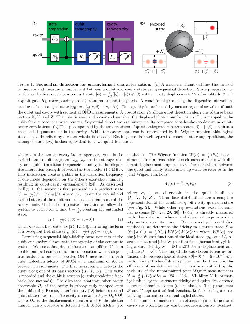
Figure 1: Sequential detection for entanglement characterization. (a) A quantum circuit outlines the methodto prepare and measure entanglement between a qubit and cavity state using sequential detection. State preparation isperformed by first creating a product state |ψ〉 = 1√

2(|g〉 + |e〉) ⊗ |β〉 with a cavity displacement Dβ of amplitude β and

a qubit gate Ryπ2

corresponding to a π2 rotation around the y-axis. A conditional gate using the dispersive interaction,

produces the entangled state |ψB〉 = 1√2(|g, β〉+ |e,−β〉). Tomography is performed by measuring an observable of both

the qubit and cavity with sequential QND measurements. A pre-rotation Ri allows qubit detection along one of three basisvectors X, Y , and Z. The qubit is reset and a cavity observable, the displaced photon number parity Pα, is mapped to thequbit for a subsequent measurement. Sequential detections are binary results compared shot-by-shot to determine qubit-cavity correlations. (b) The space spanned by the superposition of quasi-orthogonal coherent states |β〉 , |−β〉 constitutesan encoded quantum bit in the cavity. While the cavity state can be represented by its Wigner function, this logicalstate is also described by a vector within its encoded Bloch sphere. For well-separated coherent state superpositions, theentangled state |ψB〉 is then equivalent to a two-qubit Bell state.

where a is the storage cavity ladder operator, |e〉 〈e| is theexcited state qubit projector, ωs, ωq are the storage cav-ity and qubit transition frequencies, and χ is the disper-sive interaction strength between the two modes (1.4 MHz).This interaction creates a shift in the transition frequencyof one mode dependent on the other’s excitation number,resulting in qubit-cavity entanglement [24]. As describedin Fig. 1, the system is first prepared in a product state|ψ〉 = 1√

2(|g〉+ |e〉)⊗|β〉, where |g〉 , |e〉 are the ground and

excited states of the qubit and |β〉 is a coherent state of thecavity mode. Under the dispersive interaction we allow thesystem to evolve for a time t = π

χ , creating the entangledstate:

|ψB〉 = 1√2(|g, β〉+ |e,−β〉) (2)

which we call a Bell-cat state [25, 12, 13], mirroring the formof a two-qubit Bell state (e.g. |ψ〉 = 1√

2(|gg〉+ |ee〉)).

Correlating sequential high-fidelity measurements of thequbit and cavity allows state tomography of the compositesystem. We use a Josephson bifurcation amplifier [26] in adouble-pumped configuration in combination with a disper-sive readout to perform repeated QND measurements withqubit detection fidelity of 98.0% at a minimum of 800 nsbetween measurements. The first measurement detects thequbit along one of its basis vectors {X, Y, Z}. This valueis recorded and the qubit is reset to |g〉 using real-time feed-back (see methods). The displaced photon-number parityobservable Pα of the cavity is subsequently mapped ontothe qubit using Ramsey interferometry [18] before a secondqubit state detection. The cavity observable Pα = DαPD

†α

where Dα is the displacement operator and P the photonnumber parity operator is detected with 95.5% fidelity (see

methods). The Wigner function W (α) = 2π 〈Pα〉 is con-

structed from an ensemble of such measurements with dif-ferent displacement amplitudes α. The correlations betweenthe qubit and cavity states make up what we refer to as thejoint Wigner functions:

Wi(α) = 2π 〈σiPα〉 (3)

where σi is an observable in the qubit Pauli set{I, X, Y, Z}. These four distributions are a completerepresentation of the combined qubit-cavity quantum state(see Fig. 2). While other representations exist for sim-ilar systems [27, 28, 29, 30], Wi(α) is directly measuredwith this detection scheme and does not require a den-sity matrix reconstruction. By an overlap integral (seemethods), we determine the fidelity to a target state F =〈ψB| ρ |ψB〉 = π

2

∑i

∫WBi (α)Wi(α)d2α where WB

i (α) arethe joint Wigner functions of the ideal state |ψB〉 and Wi(α)are the measured joint Wigner functions (normalized), yield-ing a state fidelity F = (87 ± 2)% for a displacement am-plitude β =

√3. This amplitude was chosen to ensure or-

thogonality between logical states |〈β|−β〉|2 = 6×10−5 � 1with minimal trade-off due to photon loss. Furthermore, theefficiency of our detection scheme can be quantified by thevisibility of the unnormalized joint Wigner measurementsV = 2

π

∫〈IPα〉d2α = (85 ± 1)%. Visibility V is primar-

ily limited by measurement fidelity and qubit decoherencebetween detection events (see methods). The parametersF and V represent critical benchmarks for creating and re-trieving information from entangled states.

The number of measurement settings required to performcavity state tomography can be resource intensive. Restrict-

2

(a)

Mea

n Va

lue

(b)

1.0

-1.0

0.5

-0.5

0.0

Re( )

Im(

)

-2 0 2

-2

0

2

0 2 4 6 8 10 0 2 4 6 8 10

eg0

2

4

6

8

10

0

2

4

6

8

10

g

e

Fock state basis

Re( )

ge

ge

0.1

-0.1

0.0

Re( )0.5

0.0

(c)

Encoded basis

Figure 2: Joint Wigner tomography of a Bell-cat state. (a) The set of joint Wigner functions Wi(α) = 2π 〈σiPα〉

represents the state of a qubit-cavity system with correlations between the qubit σi = {I ,X , Y , Z} and cavity Pαreported for a state |ψB〉 and displacement amplitude β =

√3. Shown are measurements comprised of four grids of 6500

correlations between the qubit and cavity states. Interference fringes in 〈XPα〉 and 〈Y Pα〉 reveal quantum coherence inthe entangled state. (b) A density matrix reconstruction shows the combined qubit-cavity state ρ in the Fock state basis.(c) Projecting onto the logical basis |β〉 〈β| + |−β〉 〈−β|, this state can be further reduced exhibiting the traditional Bellstate form.

ing to an encoded qubit subspace, only four values of thecavity Wigner function W (α) are required to reconstruct thestate, known as a direct fidelity estimation (DFE) [20, 19].For large cat states | 〈β|−β〉 |2 � 1, the encoded state ob-servables map to cavity observables as:

Xc = P0 Ic = Pβ + P−β (4)

Yc = P jπ8β

Zc = Pβ − P−β

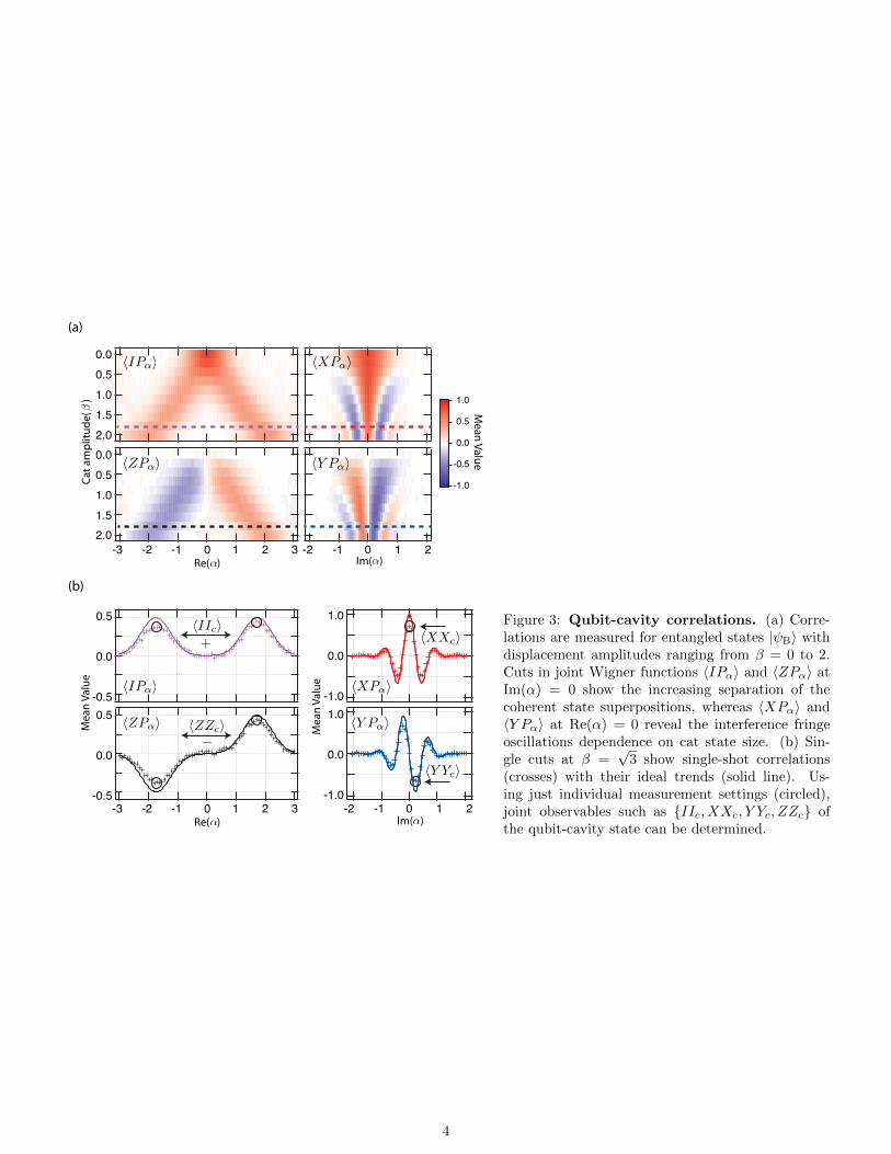
where {Ic, Xc, Yc, Zc} form the Pauli set for the encodedqubit state in the cavity (see methods). Cuts in the jointWigner function (Fig. 3) show these observables and theircorrelations to the qubit as a function of cat state size. Asthe superposition state is made larger, interference fringeoscillations increase while fringe amplitude decreases due tophoton loss. For a state |ψB〉 with |β| =

√3, we estimate a

direct fidelity FDFE = 14 (〈IIc〉+ 〈XXc〉− 〈Y Yc〉+ 〈ZZc〉) =

(72± 2)% putting a fidelity bound on the target state withno corrections for visibility. This estimate is related to thebenchmarks reported above FDFE ≈ V×F and far surpassesthe 50% threshold for a classically correlated state. Thisindicates both high fidelity state-preparation and measure-ment, and demonstrates that strong correlations are directlydetectable using joint Wigner tomography.

To place a stricter bound on observed entanglement, weperform a CHSH Bell test on the measured state. Althoughproposed to investigate local hidden variable theory, the Belltest also serves to benchmark the performance of a quantumsystem that creates and measures entangled states [8, 7, 31].Classical theory dictates that the sum of four correlationswill be bounded such that:

−2 ≤ O = 〈AAc〉+ 〈ABc〉 − 〈BAc〉+ 〈BBc〉 ≤ 2 (5)

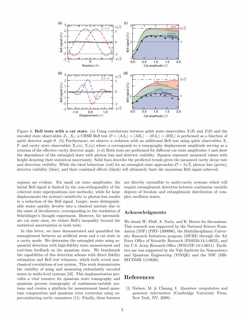
where in this experiment A,B are two qubit observablesand Ac, Bc are two cavity observables. We perform two Belltests (Fig. 4) with correlations taken shot-by-shot with nopost-selection or compensation for detector inefficiencies. Inthe first, we take observables X(θ), Z(θ), Xc, Zc and sweepboth qubit detector angle θ (see methods) and cat stateamplitude β. We observe a Bell signal with a maximal vi-olation O1 = 2.30 ± 0.04 at θ = −π4 for β = 1. In thesecond Bell test, we follow a scheme similar to Ref. [21] andchoose observables X,Y,Xc(α), Yc(α) where α is a displace-ment amplitude corresponding to a rotation of the encodedcavity state detector (see methods) and observe a maxi-mal violation O2 = 2.14 ± 0.03 for β = 1. As predicted,a lower Bell signal is observed in the second test due toits greater sensitivity to photon loss, yet in both tests two

3

(a)

(b)

0.00.51.01.52.00.00.51.01.52.0

-2 -1 0 1 2

-3 -2 -1 0 1 2 3

0.5

0.0

-0.50.5

0.0

-0.5

Re( )

Im( )

Im( )

Mean Value

1.0

-1.0

0.5

-0.5

0.0

-2 -1 0 1 2

Mea

n Va

lue

1.0

0.0

-1.01.0

0.0

-1.0

Mea

n Va

lue

-3 -2 -1 0 1 2 3Re( )

Cat a

mpl

itude

( )

Figure 3: Qubit-cavity correlations. (a) Corre-lations are measured for entangled states |ψB〉 withdisplacement amplitudes ranging from β = 0 to 2.Cuts in joint Wigner functions 〈IPα〉 and 〈ZPα〉 atIm(α) = 0 show the increasing separation of thecoherent state superpositions, whereas 〈XPα〉 and〈Y Pα〉 at Re(α) = 0 reveal the interference fringeoscillations dependence on cat state size. (b) Sin-gle cuts at β =

√3 show single-shot correlations

(crosses) with their ideal trends (solid line). Us-ing just individual measurement settings (circled),joint observables such as {IIc, XXc, Y Yc, ZZc} ofthe qubit-cavity state can be determined.

4

0Cat amplitude ( )Rotation ( )

0.50.0 1.0 1.5 2.0

Cat amplitude ( )0.50.0 1.0 1.5 2.00.0 1.0-1.0

Displacement ( )

(a)

(b)

idealphoton loss

visibility

idealphoton loss

visibility

(c)

(d)

Bell

sign

al (

)

Bell

sign

al (

)

Bell

sign

al (

)

Bell

sign

al (

)

combined

combined

Figure 4: Bell tests with a cat state. (a) Using correlations between qubit state observables X(θ) and Z(θ) and theencoded state observables Zc, Xc; a CHSH Bell test O = 〈AAc〉+ 〈ABc〉 − 〈BAc〉+ 〈BBc〉 is performed as a function ofqubit detector angle θ. (b) Furthermore, we observe a violation with an additional Bell test using qubit observables X,Y and cavity state observables Xc(α), Yc(α) where α corresponds to a tomography displacement amplitude serving as arotation of the effective cavity detector angle. (c-d) Both tests are performed for different cat state amplitudes β and showthe dependence of the entangled state with photon loss and detector visibility. Squares represent measured values withheight denoting their statistical uncertainty. Solid lines describe the predicted trends given the measured cavity decay rateand detection visibility. While the ideal behaviour (red) for an entangled state approaches O = 2

√2, photon loss (green),

detector visibility (blue), and their combined effects (black) will ultimately limit the maximum Bell signal achieved.

regimes are evident. For small cat state amplitudes, theinitial Bell signal is limited by the non-orthogonality of thecoherent state superpositions (see methods), while for largedisplacements the system’s sensitivity to photon loss resultsin a reduction of the Bell signal. Larger, more distinguish-able states quickly devolve into a classical mixture due tothe onset of decoherence, corresponding to the resolution ofSchrodinger’s thought experiment. However, for intermedi-ate cat state sizes, we violate Bell’s inequality beyond thestatistical uncertainties in both tests.

In this letter, we have demonstrated and quantified theentanglement between an artificial atom and a cat state ina cavity mode. We determine the entangled state using se-quential detection with high-fidelity state measurement andreal-time feedback on the quantum state. We benchmarkthe capabilities of this detection scheme with direct fidelityestimation and Bell test witnesses, which both reveal non-classical correlations of our system. This work demonstratesthe viability of using and measuring redundantly encodedstates in multi-level systems [16]. This implementation pro-vides a vital resource for quantum state tomography andquantum process tomography of continuous-variable sys-tems and creates a platform for measurement based quan-tum computation and quantum error correction using su-perconducting cavity resonators [11]. Finally, these features

are directly extendible to multi-cavity systems which willrequire entanglement detection between continuous variabledegrees of freedom and entanglement distribution of com-plex oscillator states.

Acknowledgments

We thank W. Pfaff, A. Narla, and R. Heeres for discussions.This research was supported by the National Science Foun-dation (NSF) (PHY-1309996), the Multidisciplinary Univer-sity Research Initiatives program (MURI) through the AirForce Office of Scientific Research (FA9550-14-1-0052), andthe U.S. Army Research Office (W911NF-14-1-0011). Facili-ties use was supported by the Yale Institute for Nanoscienceand Quantum Engineering (YINQE) and the NSF (MR-SECDMR 1119826).

References

[1] Nielsen, M. & Chuang, I. Quantum computation andquantum information (Cambridge University Press,New York, NY, 2009).

5

[2] Clauser, J. F., Horne, M. A., Shimony, A. & Holt, R. A.Proposed experiment to test local hidden-variable the-ories. Physical Review Letters 23, 880 (1969).

[3] Freedman, S. J. & Clauser, J. F. Experimental test oflocal hidden-variable theories. Physical Review Letters28, 938 (1972).

[4] Aspect, A., Grangier, P. & Roger, G. Experimentaltests of realistic local theories via Bell’s theorem. Phys-ical Review Letters 47, 460 (1981).

[5] Rowe, M. A. et al. Experimental violation of a Bell’sinequality with efficient detection. Nature 409, 791–794(2001).

[6] Hofmann, J. et al. Heralded entanglement betweenwidely separated atoms. Science 337, 72–75 (2012).

[7] Pfaff, W. et al. Demonstration of entanglement-by-measurement of solid-state qubits. Nature Physics 9,29–33 (2012).

[8] Ansmann, M. et al. Violation of Bell’s inequality inJosephson phase qubits. Nature 461, 504–506 (2009).

[9] Haroche, S. & Raimond, J.-M. Exploring the Quan-tum: Atoms, Cavities, and Photons (Oxford UniversityPress, 2006).

[10] Wallraff, A. et al. Strong coupling of a single photonto a superconducting qubit using circuit quantum elec-trodynamics. Nature 431, 162–167 (2004).

[11] Mirrahimi, M. et al. Dynamically protected cat-qubits:a new paradigm for universal quantum computation.New Journal of Physics 16, 045014 (2014).

[12] Vlastakis, B. et al. Deterministically Encoding Quan-tum Information Using 100-Photon Schrodinger CatStates. Science 342, 607–610 (2013).

[13] Sun, L. et al. Tracking photon jumps with repeatedquantum non-demolition parity measurements. Nature511, 444 (2014).

[14] Hofheinz, M. et al. Synthesizing arbitrary quantumstates in a superconducting resonator. Nature 459,546–549 (2009).

[15] DiVincenzo, D. P. The Physical Implementation ofQuantum Computation. Fortschritte der Physik 48,771 (2000).

[16] Gottesman, D., Kitaev, A. & Preskill, J. Encoding aqubit in an oscillator. Physical Review A 64, 012310(2001).

[17] Leghtas, Z. et al. Hardware-efficient autonomous quan-tum memory protection. Physical Review Letters 111,120501 (2013).

[18] Lutterbach, L. G. & Davidovich, L. Method for directmeasurement of the Wigner function in cavity QEDand ion traps. Physical Review Letters 78, 2547–2550(1997).

[19] da Silva, M., Landon-Cardinal, O. & Poulin, D. Practi-cal Characterization of Quantum Devices without To-mography. Physical Review Letters 107, 210404 (2011).

[20] Flammia, S. T. & Liu, Y.-K. Direct Fidelity Estimationfrom Few Pauli Measurements. Physical Review Letters106, 230501 (2011).

[21] Park, J., Saunders, M., Shin, Y.-i., An, K. & Jeong,H. Bell-inequality tests with entanglement between anatom and a coherent state in a cavity. Physical ReviewA 85, 022120 (2012).

[22] Paik, H. et al. Observation of high coherence in Joseph-son junction qubits measured in a three-dimensionalcircuit QED architecture. Physical Review Letters 107,240501 (2011).

[23] Kirchmair, G. et al. Observation of quantum state col-lapse and revival due to the single-photon Kerr effect.Nature 495, 205–209 (2013).

[24] Brune, M., Haroche, S., Raimond, J., Davidovich, L. &Zagury, N. Manipulation of photons in a cavity by dis-persive atom-field coupling: Quantum-nondemolitionmeasurements and generation of “Schrodinger cat”states. Physical Review A 45, 5193–5214 (1992).

[25] Brune, M. et al. Observing the Progressive Decoherenceof the “Meter” in a Quantum Measurement. PhysicalReview Letters 77, 4887–4890 (1996).

[26] Vijay, R., Devoret, M. H. & Siddiqi, I. The Josephsonbifurcation amplifier. Review of Scientific Instruments80, 111101 (2009).

[27] Eichler, C. et al. Observation of Entanglement BetweenItinerant Microwave Photons and a SuperconductingQubit. Physical Review Letters 109, 240501 (2012).

[28] Morin, O. et al. Remote creation of hybrid entangle-ment between particle-like and wave-like optical qubits.Nature Photonics 8, 570–574 (2014).

[29] Jeong, H. et al. Generation of hybrid entanglement oflight. Nature Photonics (2014).

[30] LinPeng, X. Y. et al. Joint quantum state tomographyof an entangled qubit–resonator hybrid. New Journalof Physics 15, 125027 (2013).

[31] Chow, J. et al. Detecting highly entangled states witha joint qubit readout. Physical Review A 81, 062325(2010).

[32] Kamal, A., Marblestone, A. & Devoret, M. Phys. Rev.B 79, 184301 (2009) - Signal-to-pump back action andself-oscillation in double-pump Josephson parametricamplifier. Physical Review B (2009).

[33] Murch, K. W., Weber, S. J., Macklin, C. & Siddiqi, I.Observing single quantum trajectories of a supercon-ducting quantum bit. Nature 502, 211–214 (2013).

6

[34] Nigg, S. E. et al. Black-box superconducting circuitquantization. Physical Review Letters 108, 240502(2012).

[35] Schuster, D. I. et al. Resolving photon number states ina superconducting circuit. Nature 445, 515–518 (2007).

[36] Sears, A. P. et al. Photon shot noise dephasing in thestrong-dispersive limit of circuit QED. Physical ReviewB 86, 180504 (2012).

[37] Kofman, A. G. & Korotkov, A. N. Analysis of Bellinequality violation in superconducting phase qubits.Physical Review B 77, 104502 (2008).

[38] Cahill, K. E. & Glauber, R. J. Density operators andquasiprobability distributions. Physical Review 177,1882 (1969).

[39] Smolin, J. A., Gambetta, J. M. & Smith, G. Efficientmethod for computing the maximum-likelihood quan-tum state from measurements with additive Gaussiannoise. Physical Review Letters 108, 070502 (2012).

[40] Horodecki, R., Horodecki, P., Horodecki, M. &Horodecki, K. Quantum entanglement. Reviews ofModern Physics 81, 865–942 (2009).

[41] Deleglise, S. et al. Reconstruction of non-classical cav-ity field states with snapshots of their decoherence. Na-ture 455, 510–514 (2008).

7

Supplemental Materials:Violating Bell’s inequality with an artificial atom and a cat state in a cavity

1 Materials and methods

Measurement setup: Experiments are performed in acryogen-free dilution refrigerator at a base temperature of∼ 10 mK. Our output signal amplification chain consists oftwo stages. A Josephson bifurcation amplifier (JBA) [26]operating in a double-pumping configuration [32, 33] servesas the first stage, which is followed by a high electron mo-bility transistor (HEMT) amplifier.

Fabrication techniques of the transmon qubit and the de-sign of storage and readout resonators follow the methodsdescribed in [12]. The refrigerator wiring (see Fig. S2), in-cluding the filters and attenuators used, are similar to thatof [13], but with the addition of a feedback system, the de-tails of which are discussed in a following section.

Qubit-cavity parameters: The two-cavity, single-qubitsystem is well described by the approximate dispersiveHamiltonian:

H/~ = ωsa†sas + ωra

†rar + ωqb

†b (S1)

− Ks2 a†s

2as

2 − Kr2 a†r

2ar

2 − Kq2 b†2b2

− χqsa†sasb†b− χqra†rarb†b− χrsa†sasa†rar

Where ωs,r,q are the storage, readout, and qubit transitionfrequencies, as, ar, b are the associated ladder operators, andK, χ are the modal anharmonicities and dispersive shiftsrespectively. Table 1 details the Hamiltonian parametersof our system. The resonant frequency of the readout res-onator ωr/2π is determined by transmission spectroscopy.The qubit frequency ωs/2π and storage cavity frequenciesωq/2π are found using two-tone spectroscopy.

Qubit anharmonicity Kq is measured using two-tone spec-troscopy to observe the 0 − 2 two-photon transition [22].Storage cavity anharmonicity Ks is determined by displac-ing the cavity with a coherent state and observing its timeevolution with Wigner tomography. The resulting dynamicsare characterized by state reconstruction and Ks is observedby the state’s quadratic dependence of phase on photonnumber. Finally, we predict the readout cavity anharmonic-ity Kr using its approximate dependence on the measuredvalues of Kq and the qubit-readout dispersive shift χqr [34].

The dispersive shift between the qubit and the readoutresonator χqr is found by taking the difference in frequencybetween the readout resonance when the qubit is in theground and excited state. The dispersive shift between thequbit and the storage resonator χqs is found using two meth-ods: photon number dependent qubit spectroscopy [35], andobserving qubit state revival using Ramsey interferometry[12]. Finally, χrs is predicted using its approximate rela-tionship between Ks and Kr [34].

Lifetimes and thermal populations: The lifetime ofthe storage cavity is determined by displacing to a coherentstate, waiting a variable length of time, and then applyinga qubit rotation conditioned on zero photons in the storage

cavity. This allows a measurement of the time-dependentoverlap of the cavity state with its ground state |0〉 depen-dent on time. The lifetime of the readout cavity is foundfrom its line-width. The thermal population of the qubitis determined from a histogram of one million single-shotmeasurements of the qubit thermal state, where the signal-to-noise ratio provided by the JBA allows discriminationbetween |g〉 and all states not |g〉. The thermal popula-tion of the storage cavity is found by taking the differencebetween parity measurements of the thermal and vacuumstates of the cavity. A vacuum state is prepared by firstperforming two parity measurements on the thermal stateand then post-selecting such that all results give even par-ity, projecting the thermal state onto |0〉. Finally, the knownthermal population of the readout cavity is bounded by thedephasing rate Γφ of the qubit: Γφ=nthκ, where nth is thereadout cavity’s thermal occupation and κ is the readoutsingle-photon decay rate [36].

Measurement fidelities: We define singleshot measure-

ment fidelity as Fq = P (g|g)+P (e|e)2 , where P (g|g) and P (e|e)

are the probabilities to get |g〉 (|e〉) knowing that we startwith |g〉 (|e〉). The state |g〉 is prepared through purifica-tion of the qubit thermal state with realtime feedback (seethe following section). Given a preparation of |g〉, we havea 98.5% chance of measuring |g〉 again (P (g|g) = 0.985).Likewise, we find P (e|e) = 0.975 by preparing |g〉 and rotat-ing the state to |e〉. This gives a single-shot measurementfidelity of Fq = 98%. We find our cavity parity measure-ment fidelity by purifying the storage cavity thermal stateinto |0〉 then performing one of two kinds of parity measure-ment (see Fig. 2). We report a parity measurement fidelity

for n = 0 photons as Fc = P (g|E1)+P (e|E2)2 = 95.5%, where

P (g|E1) (P (e|E2)) is the probability to measure |g〉 (|e〉)given that the parity is even for each of the two measure-ment settings. We expect Fc to decrease with increasingnumbers of photons in the cavity due to single photon lossduring the measurement sequence.

Directly from these readout fidelities, the estimated visi-bility [37] for correlated observables Vest = (2Fq − 1)(2Fc −1) = 87%. This allows us to predict the maximum Bell viola-tion possible given only measurement inefficiencies Omax =2√

2Vest = 2.47. In practice, V is directly related to thecontrast of the joint Wigner function (see Sec. 3) which wemeasure to be 85%. This discrepancy is due to qubit de-coherence, which is studied further in Sec. 2 and puts amore conservative estimate for the maximum Bell violationachievable: Omax = 2

√2V = 2.40.

I/O control parameters: As shown in Fig. S3, we em-ploy a field-programmable gate array (FPGA) in order toimplement an active feedback scheme. We use an X6-1000Mboard from Innovative Integration which contains two 1GS/s ADCs, two 1 GS/s DAC channels, and digital in-puts/outputs all controlled by a Xilinx VIRTEX-6 FPGAloaded with custom logic. We synchronize two such boards

1

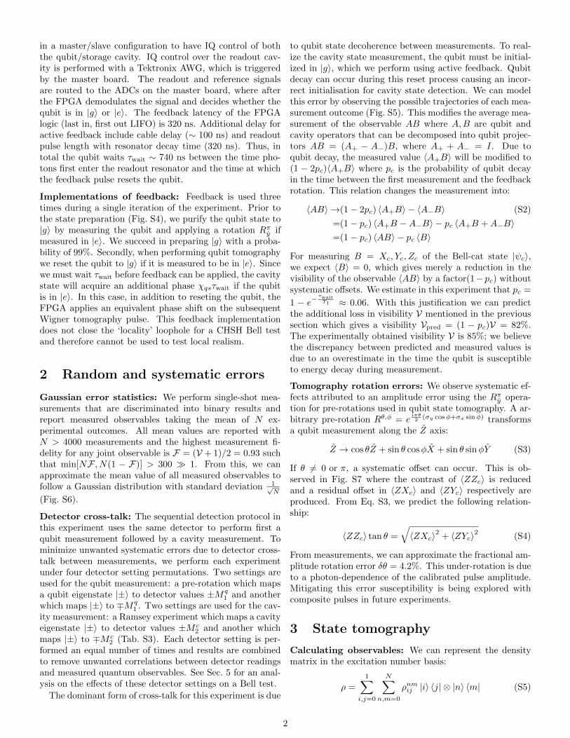
in a master/slave configuration to have IQ control of boththe qubit/storage cavity. IQ control over the readout cav-ity is performed with a Tektronix AWG, which is triggeredby the master board. The readout and reference signalsare routed to the ADCs on the master board, where afterthe FPGA demodulates the signal and decides whether thequbit is in |g〉 or |e〉. The feedback latency of the FPGAlogic (last in, first out LIFO) is 320 ns. Additional delay foractive feedback include cable delay (∼ 100 ns) and readoutpulse length with resonator decay time (320 ns). Thus, intotal the qubit waits τwait ∼ 740 ns between the time pho-tons first enter the readout resonator and the time at whichthe feedback pulse resets the qubit.

Implementations of feedback: Feedback is used threetimes during a single iteration of the experiment. Prior tothe state preparation (Fig. S4), we purify the qubit state to|g〉 by measuring the qubit and applying a rotation Rπy ifmeasured in |e〉. We succeed in preparing |g〉 with a proba-bility of 99%. Secondly, when performing qubit tomographywe reset the qubit to |g〉 if it is measured to be in |e〉. Sincewe must wait τwait before feedback can be applied, the cavitystate will acquire an additional phase χqsτwait if the qubitis in |e〉. In this case, in addition to reseting the qubit, theFPGA applies an equivalent phase shift on the subsequentWigner tomography pulse. This feedback implementationdoes not close the ‘locality’ loophole for a CHSH Bell testand therefore cannot be used to test local realism.

2 Random and systematic errors

Gaussian error statistics: We perform single-shot mea-surements that are discriminated into binary results andreport measured observables taking the mean of N ex-perimental outcomes. All mean values are reported withN > 4000 measurements and the highest measurement fi-delity for any joint observable is F = (V + 1)/2 = 0.93 suchthat min[NF , N(1 − F)] > 300 � 1. From this, we canapproximate the mean value of all measured observables tofollow a Gaussian distribution with standard deviation 1√

N

(Fig. S6).

Detector cross-talk: The sequential detection protocol inthis experiment uses the same detector to perform first aqubit measurement followed by a cavity measurement. Tominimize unwanted systematic errors due to detector cross-talk between measurements, we perform each experimentunder four detector setting permutations. Two settings areused for the qubit measurement: a pre-rotation which mapsa qubit eigenstate |±〉 to detector values ±Mq

1 and anotherwhich maps |±〉 to ∓Mq

1 . Two settings are used for the cav-ity measurement: a Ramsey experiment which maps a cavityeigenstate |±〉 to detector values ±M c

2 and another whichmaps |±〉 to ∓M c

2 (Tab. S3). Each detector setting is per-formed an equal number of times and results are combinedto remove unwanted correlations between detector readingsand measured quantum observables. See Sec. 5 for an anal-ysis on the effects of these detector settings on a Bell test.

The dominant form of cross-talk for this experiment is due

to qubit state decoherence between measurements. To real-ize the cavity state measurement, the qubit must be initial-ized in |g〉, which we perform using active feedback. Qubitdecay can occur during this reset process causing an incor-rect initialisation for cavity state detection. We can modelthis error by observing the possible trajectories of each mea-surement outcome (Fig. S5). This modifies the average mea-surement of the observable AB where A,B are qubit andcavity operators that can be decomposed into qubit projec-tors AB = (A+ − A−)B, where A+ + A− = I. Due toqubit decay, the measured value 〈A+B〉 will be modified to(1 − 2pc)〈A+B〉 where pc is the probability of qubit decayin the time between the first measurement and the feedbackrotation. This relation changes the measurement into:

〈AB〉 →(1− 2pc) 〈A+B〉 − 〈A−B〉 (S2)

=(1− pc) 〈A+B −A−B〉 − pc 〈A+B +A−B〉=(1− pc) 〈AB〉 − pc 〈B〉

For measuring B = Xc, Yc, Zc of the Bell-cat state |ψc〉,we expect 〈B〉 = 0, which gives merely a reduction in thevisibility of the observable 〈AB〉 by a factor(1−pc) withoutsystematic offsets. We estimate in this experiment that pc =

1 − e−τwaitT1 ≈ 0.06. With this justification we can predict

the additional loss in visibility V mentioned in the previoussection which gives a visibility Vpred = (1 − pc)V = 82%.The experimentally obtained visibility V is 85%; we believethe discrepancy between predicted and measured values isdue to an overestimate in the time the qubit is susceptibleto energy decay during measurement.

Tomography rotation errors: We observe systematic ef-fects attributed to an amplitude error using the Rπy opera-tion for pre-rotations used in qubit state tomography. A ar-bitrary pre-rotation Rθ,φ = e

iπθ2 (σy cosφ+σx sinφ) transforms

a qubit measurement along the Z axis:

Z → cos θZ + sin θ cosφX + sin θ sinφY (S3)

If θ 6= 0 or π, a systematic offset can occur. This is ob-served in Fig. S7 where the contrast of 〈ZZc〉 is reducedand a residual offset in 〈ZXc〉 and 〈ZYc〉 respectively areproduced. From Eq. S3, we predict the following relation-ship:

〈ZZc〉 tan θ =

√〈ZXc〉2 + 〈ZYc〉2 (S4)

From measurements, we can approximate the fractional am-plitude rotation error δθ = 4.2%. This under-rotation is dueto a photon-dependence of the calibrated pulse amplitude.Mitigating this error susceptibility is being explored withcomposite pulses in future experiments.

3 State tomography

Calculating observables: We can represent the densitymatrix in the excitation number basis:

ρ =

1∑i,j=0

N∑n,m=0

ρnmij |i〉 〈j| ⊗ |n〉 〈m| (S5)

2

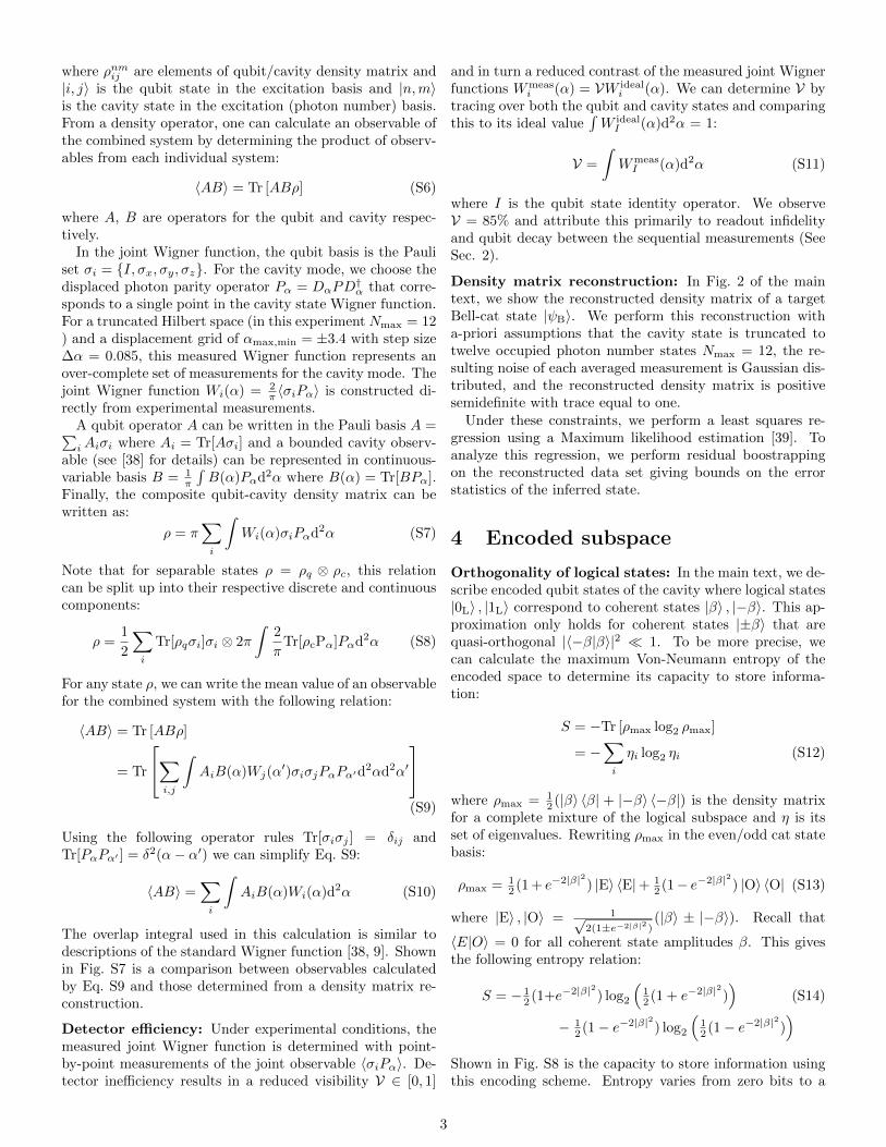
where ρnmij are elements of qubit/cavity density matrix and|i, j〉 is the qubit state in the excitation basis and |n,m〉is the cavity state in the excitation (photon number) basis.From a density operator, one can calculate an observable ofthe combined system by determining the product of observ-ables from each individual system:

〈AB〉 = Tr [ABρ] (S6)

where A, B are operators for the qubit and cavity respec-tively.

In the joint Wigner function, the qubit basis is the Pauliset σi = {I, σx, σy, σz}. For the cavity mode, we choose thedisplaced photon parity operator Pα = DαPD

†α that corre-

sponds to a single point in the cavity state Wigner function.For a truncated Hilbert space (in this experiment Nmax = 12) and a displacement grid of αmax,min = ±3.4 with step size∆α = 0.085, this measured Wigner function represents anover-complete set of measurements for the cavity mode. Thejoint Wigner function Wi(α) = 2

π 〈σiPα〉 is constructed di-rectly from experimental measurements.

A qubit operator A can be written in the Pauli basis A =∑iAiσi where Ai = Tr[Aσi] and a bounded cavity observ-

able (see [38] for details) can be represented in continuous-variable basis B = 1

π

∫B(α)Pαd2α where B(α) = Tr[BPα].

Finally, the composite qubit-cavity density matrix can bewritten as:

ρ = π∑i

∫Wi(α)σiPαd2α (S7)

Note that for separable states ρ = ρq ⊗ ρc, this relationcan be split up into their respective discrete and continuouscomponents:

ρ =1

2

∑i

Tr[ρqσi]σi ⊗ 2π

∫2

πTr[ρcPα]Pαd2α (S8)

For any state ρ, we can write the mean value of an observablefor the combined system with the following relation:

〈AB〉 = Tr [ABρ]

= Tr

∑i,j

∫AiB(α)Wj(α

′)σiσjPαPα′d2αd2α′

(S9)

Using the following operator rules Tr[σiσj ] = δij andTr[PαPα′ ] = δ2(α− α′) we can simplify Eq. S9:

〈AB〉 =∑i

∫AiB(α)Wi(α)d2α (S10)

The overlap integral used in this calculation is similar todescriptions of the standard Wigner function [38, 9]. Shownin Fig. S7 is a comparison between observables calculatedby Eq. S9 and those determined from a density matrix re-construction.

Detector efficiency: Under experimental conditions, themeasured joint Wigner function is determined with point-by-point measurements of the joint observable 〈σiPα〉. De-tector inefficiency results in a reduced visibility V ∈ [0, 1]

and in turn a reduced contrast of the measured joint Wignerfunctions Wmeas

i (α) = VW ideali (α). We can determine V by

tracing over both the qubit and cavity states and comparingthis to its ideal value

∫W idealI (α)d2α = 1:

V =

∫WmeasI (α)d2α (S11)

where I is the qubit state identity operator. We observeV = 85% and attribute this primarily to readout infidelityand qubit decay between the sequential measurements (SeeSec. 2).

Density matrix reconstruction: In Fig. 2 of the maintext, we show the reconstructed density matrix of a targetBell-cat state |ψB〉. We perform this reconstruction witha-priori assumptions that the cavity state is truncated totwelve occupied photon number states Nmax = 12, the re-sulting noise of each averaged measurement is Gaussian dis-tributed, and the reconstructed density matrix is positivesemidefinite with trace equal to one.

Under these constraints, we perform a least squares re-gression using a Maximum likelihood estimation [39]. Toanalyze this regression, we perform residual boostrappingon the reconstructed data set giving bounds on the errorstatistics of the inferred state.

4 Encoded subspace

Orthogonality of logical states: In the main text, we de-scribe encoded qubit states of the cavity where logical states|0L〉 , |1L〉 correspond to coherent states |β〉 , |−β〉. This ap-proximation only holds for coherent states |±β〉 that arequasi-orthogonal |〈−β|β〉|2 � 1. To be more precise, wecan calculate the maximum Von-Neumann entropy of theencoded space to determine its capacity to store informa-tion:

S = −Tr [ρmax log2 ρmax]

= −∑i

ηi log2 ηi (S12)

where ρmax = 12 (|β〉 〈β| + |−β〉 〈−β|) is the density matrix

for a complete mixture of the logical subspace and η is itsset of eigenvalues. Rewriting ρmax in the even/odd cat statebasis:

ρmax = 12 (1 + e−2|β|2) |E〉 〈E|+ 1

2 (1− e−2|β|2) |O〉 〈O| (S13)

where |E〉 , |O〉 = 1√2(1±e−2|β|2 )

(|β〉 ± |−β〉). Recall that

〈E|O〉 = 0 for all coherent state amplitudes β. This givesthe following entropy relation:

S = − 12 (1+e−2|β|2) log2

(12 (1 + e−2|β|2)

)(S14)

− 12 (1− e−2|β|2) log2

(12 (1− e−2|β|2)

)Shown in Fig. S8 is the capacity to store information usingthis encoding scheme. Entropy varies from zero bits to a

3

value asymptotically approaching a single bit with increas-ing coherent state amplitudes β. The orthogonality betweenlogical states |〈β| − β〉|2 is directly related to this informa-tion capacity and serves as a proxy for validating the qubitapproximation of the produced cavity state.

4.1 Encoded state observables

The coherent state basis chosen in this report to representthe encoded qubit has Pauli operators:

Xc = |−β〉 〈β|+ |β〉 〈−β| (S15)

Yc = j |−β〉 〈β| − j |β〉 〈−β|Zc = |β〉 〈β| − |−β〉 〈−β|Ic = |β〉 〈β|+ |−β〉 〈−β|

Here, we will show that the operators expressed in Eq. 4of the main text, approximate these encoded Pauli opera-tors. Assuming 〈β|−β〉 � 1, we have the following photon-number parity P relations:

〈β|P0 |β〉 = 〈β|−β〉 � 1 (S16)

〈β|P0 |−β〉 = 〈β|β〉 = 1

〈β|Pα |β〉 = 〈β − α|α− β〉 � 1

〈β|Pα |−β〉 = e2(αβ∗−α∗β) 〈α|−α〉

where Pα = DαPD−α for some displacement amplitude α.Now taking the projector M = |β〉 〈β|+|−β〉 〈−β|, we derivethe encoded state’s Pauli Operators from the cavity stateobservables reported in Eq. 4 of the main text:

MP0M† ≈ |−β〉 〈β|+ |β〉 〈−β| (S17)

MPβM† ≈ |β〉 〈β|

MP−βM† ≈ |−β〉 〈−β|

MP jπ8βM† ≈ j |−β〉 〈β| − j |β〉 〈−β|

Putting these relationships together, as in Eq. 4, builds theencoded state observables {Xc, Yc, Zc, Ic} and reveals thatthese observables can be efficiently measured using Wignertomography. Ic and Zc require a comparison between twodifferent observables. For true single-shot readout of theselogical observable Zc, measuring a single value in the cavitystate Husimi-Q distribution Q(β) = 1

π 〈β|ρ|β〉 can be em-ployed where Zc = 2πQ(β) − 1. This is being explored infuture experiments.

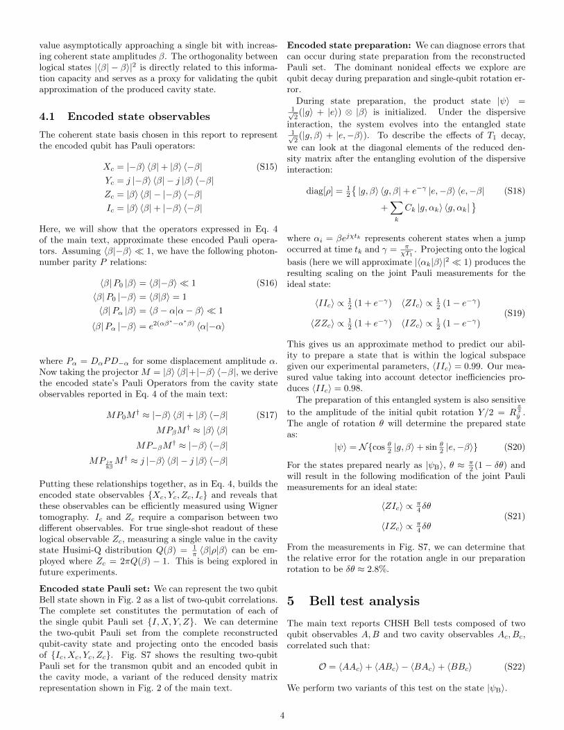
Encoded state Pauli set: We can represent the two qubitBell state shown in Fig. 2 as a list of two-qubit correlations.The complete set constitutes the permutation of each ofthe single qubit Pauli set {I,X, Y, Z}. We can determinethe two-qubit Pauli set from the complete reconstructedqubit-cavity state and projecting onto the encoded basisof {Ic, Xc, Yc, Zc}. Fig. S7 shows the resulting two-qubitPauli set for the transmon qubit and an encoded qubit inthe cavity mode, a variant of the reduced density matrixrepresentation shown in Fig. 2 of the main text.

Encoded state preparation: We can diagnose errors thatcan occur during state preparation from the reconstructedPauli set. The dominant nonideal effects we explore arequbit decay during preparation and single-qubit rotation er-ror.

During state preparation, the product state |ψ〉 =1√2(|g〉 + |e〉) ⊗ |β〉 is initialized. Under the dispersive

interaction, the system evolves into the entangled state1√2(|g, β〉 + |e,−β〉). To describe the effects of T1 decay,

we can look at the diagonal elements of the reduced den-sity matrix after the entangling evolution of the dispersiveinteraction:

diag[ρ] = 12

{|g, β〉 〈g, β|+ e−γ |e,−β〉 〈e,−β| (S18)

+∑k

Ck |g, αk〉 〈g, αk|}

where αi = βejχtk represents coherent states when a jumpoccurred at time tk and γ = π

χT1. Projecting onto the logical

basis (here we will approximate |〈αk|β〉|2 � 1) produces theresulting scaling on the joint Pauli measurements for theideal state:

〈IIc〉 ∝ 12 (1 + e−γ) 〈ZIc〉 ∝ 1

2 (1− e−γ)

〈ZZc〉 ∝ 12 (1 + e−γ) 〈IZc〉 ∝ 1

2 (1− e−γ)(S19)

This gives us an approximate method to predict our abil-ity to prepare a state that is within the logical subspacegiven our experimental parameters, 〈IIc〉 = 0.99. Our mea-sured value taking into account detector inefficiencies pro-duces 〈IIc〉 = 0.98.

The preparation of this entangled system is also sensitive

to the amplitude of the initial qubit rotation Y/2 = Rπ2

y .The angle of rotation θ will determine the prepared stateas:

|ψ〉 = N{cos θ2 |g, β〉+ sin θ2 |e,−β〉} (S20)

For the states prepared nearly as |ψB〉, θ ≈ π2 (1 − δθ) and

will result in the following modification of the joint Paulimeasurements for an ideal state:

〈ZIc〉 ∝ π4 δθ

〈IZc〉 ∝ π4 δθ

(S21)

From the measurements in Fig. S7, we can determine thatthe relative error for the rotation angle in our preparationrotation to be δθ ≈ 2.8%.

5 Bell test analysis

The main text reports CHSH Bell tests composed of twoqubit observables A,B and two cavity observables Ac, Bc,correlated such that:

O = 〈AAc〉+ 〈ABc〉 − 〈BAc〉+ 〈BBc〉 (S22)

We perform two variants of this test on the state |ψB〉.

4

Test #1 Model: In the first test we choose qubit cavityobservables Zc, Xc and qubit observables Z(θ), X(θ) where:

Z(θ) = Z cos θ2 −X sin θ2 X(θ) = X cos θ2 + Z sin θ

2(S23)

This angle θ corresponds to a rotation of the qubit statebefore detection. In Fig. 4a, we plot O for each of the fourpermutations of the joint observables and find a maximumBell violation for an angle θ = −π4 giving observables:

A = X+Z√2

; B = X−Z√2

Ac = Zc; Bc = Xc(S24)

As shown in Fig. 4c, we can model the effects of photonloss and measurement inefficiency on the maximum viola-tion. For the ideal case, an overlap of the coherent statesuperposition reduces contrast in 〈AZc〉 and 〈BZc〉 and willlimit the maximum Bell signal:

Oideal =√

2(2− e−8|β|2)

Measurement inefficiency will reduce the contrast of thismaximum Bell signal which we expect to go as the visibilityV:

Ovis =√

2V(2− e−8|β|2)

Photon loss will also have an effect on the maximum Bellsignal by reducing the measured contrast of all correlationsfor 〈AXc〉 and 〈BXc〉. This produces the an amplitude de-pendent maximum Bell Signal:

Oloss =√

2(1− e−8|β|2 − e−2|β|2γ)

where γ = teffτs

such that τs is the photon decay time constantand teff is the effective time to create and measure the Bell-cat state. Finally taking into account both visibility andphoton loss produces the expected maximum Bell signal:

Opred =√

2V(1− e−8|β|2 − e−2γ|β|2)

This predicted Bell signal is shown in Fig. 4 of the main textusing the measured joint-Wigner contrast V = 0.85 and timebetween cavity state creation and detection teff = 1.24 µs.

Test #2 Model: In the second test, we choose qubit ob-servables X,Y and cavity observables Xc(α), Yc(α) where:

Xc(α) = DjαP0D†jα ≈ Xc cos α

4β + Yc sin α4β (S25)

Yc(α) = DjαP jπ8βD†jα ≈ Yc cos α

4β −Xc sin α4β

Where the displacement amplitude α corresponds to an ap-proximate rotation of the encoded cavity state before detec-tion. In Fig. 4b, we plot O for each of the four permutationsof the joint observables and find a maximum Bell violationfor a displacement α = 0.15 for β = 1 which produces theapproximate observables:

A = X; B = YAc = Xc+Yc√

2Bc = Xc−Yc√

2

(S26)

Shown in Fig. 4c, we can also model the effects of photonloss and measurement inefficiency for the second test. The

ideal case is the result of four summed joint Wigner valuesrepresented as:

Oideal = 2(cos 4α0β + sin 4α0β)e−2|α0|2

where α0 is an optimal displacement for maximum viola-tion which can be calculated from Eq. S27 and in detail inRef. [21]. Taking into account photon loss and measurementinefficiency produces the following relationship:

Opred = 2Ve−2γ|β|2(cos 4α0β + sin 4α0β)e−2|α0|2

This predicted Bell signal is shown in Fig. 4b of the maintext using the measured joint-Wigner contrast V = 0.85 andan effective time teff = 1.24 µs.

Optimal measurements for encoded observables:Eq. 3 of the main text describes the ideal observables toefficiently determine an encoded qubit state observable us-ing a superposition state with |β| � 1. In fact, the optimalmeasurement for particular observables will be further mod-ified for smaller coherent displacements.

For the second CHSH experiment, the optimal observableP±jα0

∼ 1√2(Xc ± Yc) follows the relation:

β − α0

β + α0= tan 4α0β (S27)

where α0 is the amplitude for a coherent displacement Djα0

to perform the measurement Pjα0 given β. Further detailsare discussed in Ref. [21]. In the large β limit, the observablecorresponds to the encoded qubit state observable 1√

2(Xc +

Yc) and follows the relationship Pα= jπ16β

as related in Eq. 4 of

the main text. Shown in Fig. S9 is the predicted and chosenoptimal values for a maximum CHSH Bell signal.

Two-qubit entanglement witnesses: Two qubit entan-glement can also be quantified by an entanglement wit-ness W = IIc − XXc + Y Yc − ZZc [40] for a Bell state|ψ〉 = 1√

2(|gg〉+ |ee〉). The witness ‘confirms’ entanglement

for all observations of 〈W〉 < 0. Shown in Fig. S10, we reportW (as well as its corresponding direct fidelity estimation F)as a function of coherent state amplitude β using the optimaldisplacements described in Fig. S9. As expected, entangle-ment is not detected for a β = 0 coherent state (a productstate 1√

2(|g〉+ |e〉)⊗ |0〉).

Bell test for each detector setting: We analyze thesystematic errors that can occur from a particular detectorsetting. Shown in Fig. 5 are the observables used to cal-culated a Bell violation using test #2 for each of the fourdetector settings Sec. 2. Systematic errors are shown to bewithin stastical bounds of the experiment and each detectorsetting violates Bell’s inequality by at least three standarddeviations, see Fig. 5. In the main text, we report mea-surements from the combined data set resulting in smallerstatistical error and a stronger violation of Bell’s inequality.

5

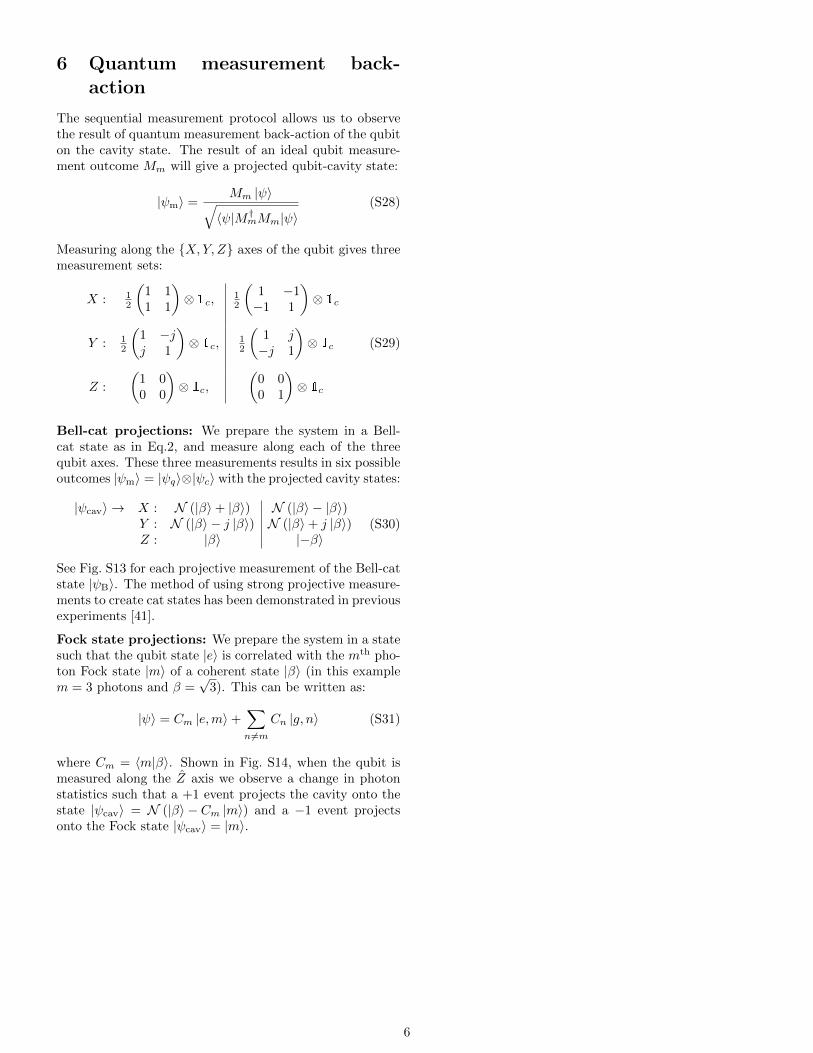
6 Quantum measurement back-action

The sequential measurement protocol allows us to observethe result of quantum measurement back-action of the qubiton the cavity state. The result of an ideal qubit measure-ment outcome Mm will give a projected qubit-cavity state:

|ψm〉 =Mm |ψ〉√〈ψ|M†mMm|ψ〉

(S28)

Measuring along the {X,Y, Z} axes of the qubit gives threemeasurement sets:

X : 12

(1 11 1

)⊗ 1c, 1

2

(1 −1−1 1

)⊗ 1c

Y : 12

(1 −jj 1

)⊗ 1c, 1

2

(1 j−j 1

)⊗ 1c

Z :

(1 00 0

)⊗ 1c,

(0 00 1

)⊗ 1c

(S29)

Bell-cat projections: We prepare the system in a Bell-cat state as in Eq.2, and measure along each of the threequbit axes. These three measurements results in six possibleoutcomes |ψm〉 = |ψq〉⊗|ψc〉 with the projected cavity states:

|ψcav〉 → X : N (|β〉+ |β〉) N (|β〉 − |β〉)Y : N (|β〉 − j |β〉) N (|β〉+ j |β〉)Z : |β〉 |−β〉

(S30)

See Fig. S13 for each projective measurement of the Bell-catstate |ψB〉. The method of using strong projective measure-ments to create cat states has been demonstrated in previousexperiments [41].

Fock state projections: We prepare the system in a statesuch that the qubit state |e〉 is correlated with the mth pho-ton Fock state |m〉 of a coherent state |β〉 (in this examplem = 3 photons and β =

√3). This can be written as:

|ψ〉 = Cm |e,m〉+∑n 6=m

Cn |g, n〉 (S31)

where Cm = 〈m|β〉. Shown in Fig. S14, when the qubit ismeasured along the Z axis we observe a change in photonstatistics such that a +1 event projects the cavity onto thestate |ψcav〉 = N (|β〉 − Cm |m〉) and a −1 event projectsonto the Fock state |ψcav〉 = |m〉.

6

Figure S1: Photograph of device and amplifier: (a) One half of the 3D circuit QED device shows both the readoutand storage cavities. Strongly coupled to each cavity is a single vertical transmon. (b) High-fidelity measurements areachieved with near quantum-limited amplification provided by a Josephson bifurcation amplifier. Shown is the chip andsample holder for this device.

20 dB

directionalcoupler

10 dB

TN

HEMT=5 K

10 m

K4

K29

0K

20 dB

10 dB

coax

coaxcouplers

Device

50 Ω

20 dB

isolators

JBApump

20 dB

JBA

10 dB

Storage input

Qubit andreadout input

Readoutoutput

Feedback setup

20 dB

Figure S2: Experiment Schematic

7

12S

Feedback

ωμw Storage

Storage input

Qubit andreadout input

Readoutoutput

Feedback setup

IQ

12S

ωμw Readout

ωμw

LO

1 2S

ωμw Qubit

ADC

PCIe

FPGA

DIGITAL

DAC

ADC

PCIe

FPGA

DIGITAL

AWG PC

I/O board

SwitchTO FRIDGE FROM

FRIDGE

290

K

Mixer

I/O board IQ

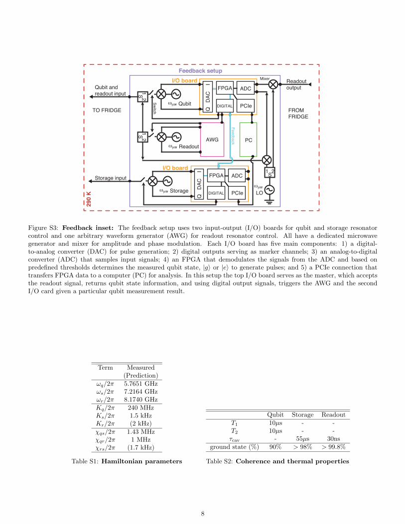
DAC

Figure S3: Feedback inset: The feedback setup uses two input-output (I/O) boards for qubit and storage resonatorcontrol and one arbitrary waveform generator (AWG) for readout resonator control. All have a dedicated microwavegenerator and mixer for amplitude and phase modulation. Each I/O board has five main components: 1) a digital-to-analog converter (DAC) for pulse generation; 2) digital outputs serving as marker channels; 3) an analog-to-digitalconverter (ADC) that samples input signals; 4) an FPGA that demodulates the signals from the ADC and based onpredefined thresholds determines the measured qubit state, |g〉 or |e〉 to generate pulses; and 5) a PCIe connection thattransfers FPGA data to a computer (PC) for analysis. In this setup the top I/O board serves as the master, which acceptsthe readout signal, returns qubit state information, and using digital output signals, triggers the AWG and the secondI/O card given a particular qubit measurement result.

Term Measured(Prediction)

ωq/2π 5.7651 GHzωs/2π 7.2164 GHzωr/2π 8.1740 GHzKq/2π 240 MHzKs/2π 1.5 kHzKr/2π (2 kHz)χqs/2π 1.43 MHzχqr/2π 1 MHzχrs/2π (1.7 kHz)

Table S1: Hamiltonian parameters

Qubit Storage ReadoutT1 10µs - -T2 10µs - -τcav - 55µs 30ns

ground state (%) 90% > 98% > 99.8%

Table S2: Coherence and thermal properties

8

cavity

qubit

(a) (b) (c) (d)

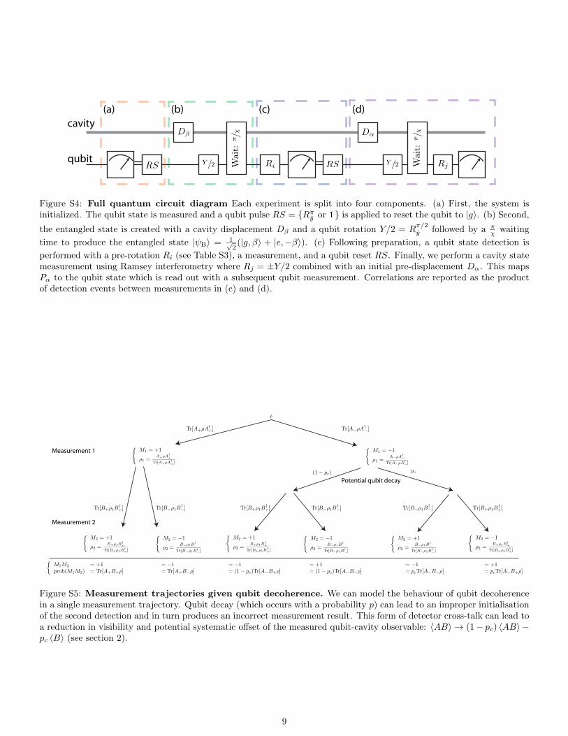
Figure S4: Full quantum circuit diagram Each experiment is split into four components. (a) First, the system isinitialized. The qubit state is measured and a qubit pulse RS = {Rπy or 1} is applied to reset the qubit to |g〉. (b) Second,

the entangled state is created with a cavity displacement Dβ and a qubit rotation Y/2 = Rπ/2y followed by a π

χ waiting

time to produce the entangled state |ψB〉 = 1√2(|g, β〉 + |e,−β〉). (c) Following preparation, a qubit state detection is

performed with a pre-rotation Ri (see Table S3), a measurement, and a qubit reset RS. Finally, we perform a cavity statemeasurement using Ramsey interferometry where Rj = ±Y/2 combined with an initial pre-displacement Dα. This mapsPα to the qubit state which is read out with a subsequent qubit measurement. Correlations are reported as the productof detection events between measurements in (c) and (d).

Potential qubit decay

Measurement 1

Measurement 2

Figure S5: Measurement trajectories given qubit decoherence. We can model the behaviour of qubit decoherencein a single measurement trajectory. Qubit decay (which occurs with a probability p) can lead to an improper initialisationof the second detection and in turn produces an incorrect measurement result. This form of detector cross-talk can lead toa reduction in visibility and potential systematic offset of the measured qubit-cavity observable: 〈AB〉 → (1− pc) 〈AB〉 −pc 〈B〉 (see section 2).

9

0.06 0.04 0.02 0.00 0.02 0.04 0.06

Residuals from reconstruction (δWi(α))

0

5

10

15

20

25C

ounts×1

02

Figure S6: Histogram of reconstruction residuals.Plotted are the residuals corresponding to the density ma-trix reconstruction of the Bell cat state shown in Fig. 2 ofthe main text. This Histogram shows the distribution of the25, 000 residuals from the joint Wigner function which givesa Gaussian distribution (mean value µ = 7.0 × 10−4, stan-dard deviation σ = 0.015), which agree with our expectationfor statistical error σest = 1√

N≈ 0.015.

Qubit CavityRi M1 Rj M2

1 +Z Rπ/2y +Pα

Rπy −Z R−π/2y −Pα

Rπ/2y +X

R−π/2y −X

R−π/2x +Y

Rπ/2x −Y

Table S3: Table of measurement operators.As shown in Fig. S4, pre-rotations before qubitand cavity state measurements determine the mea-sured observable. Shown are the different pre-rotations used and the corresponding measure-ment operator.

ˆIIcˆIXc

ˆIYcˆIZc XIc

ˆYIc ZIcˆXXc XYc

ˆXZcˆYXc

ˆYYcˆYZc

ˆZXcˆZYc

ˆZZc

Joint Pauli operator

1.0

0.5

0.0

0.5

1.0

Mean v

alu

e

Figure S7: Reconstructed Pauli sets. The set of sixteen joint Pauli operators span the two-qubit Hilbert space of thequbit/encoded-qubit state. Shown is the Pauli set for the entangled target state |ψB〉 derived in two ways. (Red) is thereconstructed Pauli set using a density matrix reconstruction of the full quantum state with no normalization constraint,then projecting onto the encoded subspace. (Blue) shows the values discerned from an overlap integral of the measuredjoint-Wigner functions (Eq. S9). These measurements agree with each other within statistical errors.

10

0.0 0.5 1.0 1.5 2.0 2.5 3.0

Displacement β

0.0

0.2

0.4

0.6

0.8

1.0

Entr

opy (

bit

s)

0.0 0.5 1.0 1.5 2.0 2.5 3.00.0

0.2

0.4

0.6

0.8

1.0

1−|⟨ β|−

β⟩ |2

0.00.1

dev.

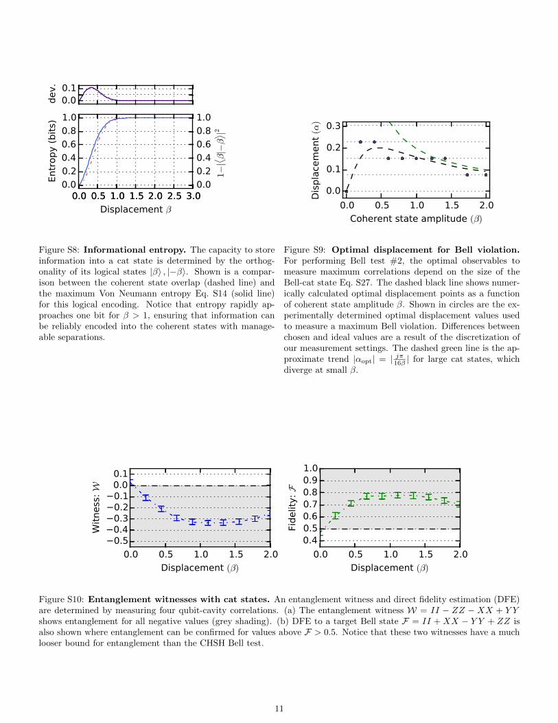
Figure S8: Informational entropy. The capacity to storeinformation into a cat state is determined by the orthog-onality of its logical states |β〉 , |−β〉. Shown is a compar-ison between the coherent state overlap (dashed line) andthe maximum Von Neumann entropy Eq. S14 (solid line)for this logical encoding. Notice that entropy rapidly ap-proaches one bit for β > 1, ensuring that information canbe reliably encoded into the coherent states with manage-able separations.

0.0 0.5 1.0 1.5 2.0

Coherent state amplitude (β)

0.0

0.1

0.2

0.3

Dis

pla

cem

ent

(α)

Figure S9: Optimal displacement for Bell violation.For performing Bell test #2, the optimal observables tomeasure maximum correlations depend on the size of theBell-cat state Eq. S27. The dashed black line shows numer-ically calculated optimal displacement points as a functionof coherent state amplitude β. Shown in circles are the ex-perimentally determined optimal displacement values usedto measure a maximum Bell violation. Differences betweenchosen and ideal values are a result of the discretization ofour measurement settings. The dashed green line is the ap-proximate trend |αopt| = | jπ16β | for large cat states, whichdiverge at small β.

0.0 0.5 1.0 1.5 2.0

Displacement (β)

0.50.40.30.20.10.00.1

Wit

ness

: W

0.0 0.5 1.0 1.5 2.0

Displacement (β)

0.40.50.60.70.80.91.0

Fidelit

y: F

Figure S10: Entanglement witnesses with cat states. An entanglement witness and direct fidelity estimation (DFE)are determined by measuring four qubit-cavity correlations. (a) The entanglement witness W = II − ZZ − XX + Y Yshows entanglement for all negative values (grey shading). (b) DFE to a target Bell state F = II + XX − Y Y + ZZ isalso shown where entanglement can be confirmed for values above F > 0.5. Notice that these two witnesses have a muchlooser bound for entanglement than the CHSH Bell test.

11

Figure S11: Observables from each detector setting.To ensure that a particular detector setting is not producingsystematic errors we have not taken into account. We reporta Bell test for each detector setting used to observe ourmaximum violation in test #2. The expectation value ofeach observable used in that Bell test is shown for the fourdetector settings used Sec. 2. Significant deviations due tounexpected systematic errors are not observed.

+ + +− −+ −−Detector setting

1.8

1.9

2.0

2.1

2.2

2.3

OC

HSH

Figure S12: Bell test for each detector setting. A Belltest is analyzed for each detector setting to determine theeffects of possible systematic errors. Each of these subtestsviolate Bell’s inequality by more than three standard devi-ations of their statistical error.

2 0 2

2

0

2

Im(α

)

+Z Projection

2 0 2

2

0

2

+X Projection

2 0 2

2

0

2

+Y Projection

2 0 2

Re(α)

2

0

2

Im(α

)

−Z Projection

2 0 2

Re(α)

2

0

2

−X Projection

2 0 2

Re(α)

2

0

2

−Y Projection

1.0

0.5

0.0

0.5

1.0

Pα

Figure S13: Qubit measurement back-action of a Bell-cat state. The resulting projections of the state |ψB〉 =1√2(|g, β〉+ |e,−β〉) due to a particular qubit measurement outcome. Note that measuring along the X and Y axes results

in a projected cat state each with different superposition phases. Combining these measurements with the probability toobtain each result describes the entire system and is used to create the joint Wigner function representation in Fig. 2 ofthe main text.

12

2 0 2

Re(α)

2

0

2

Im(α

)

2 0 2

Re(α)

2

0

2

2 0 2

Re(α)

2

0

2

0 2 4 6 8

Photon number |n⟩0.0

0.2

0.4

Pro

babili

ty

0 2 4 6 8

Photon number |n⟩0.0

0.20.40.60.8

0 2 4 6 8

Photon number |n⟩0.0

0.2

0.4

1.0

0.5

0.0

0.5

1.0

Pα

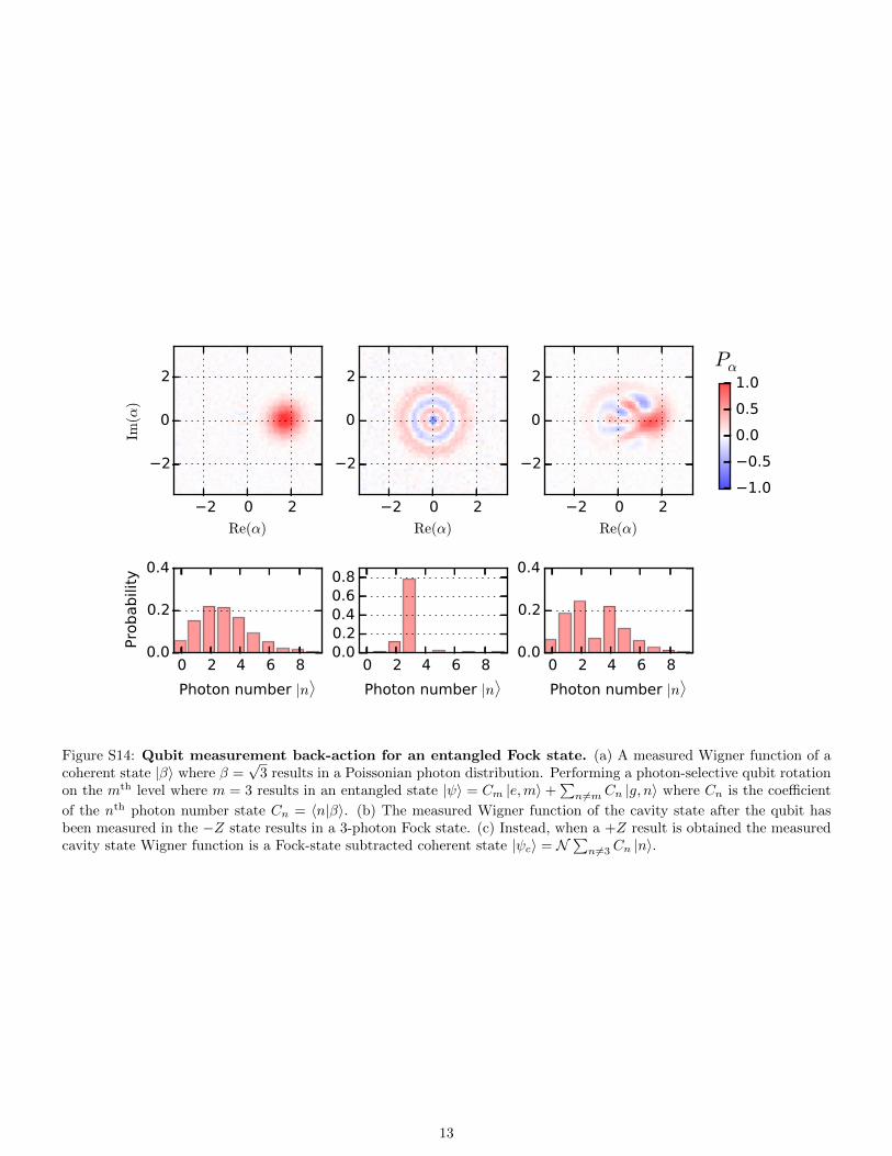
Figure S14: Qubit measurement back-action for an entangled Fock state. (a) A measured Wigner function of acoherent state |β〉 where β =

√3 results in a Poissonian photon distribution. Performing a photon-selective qubit rotation

on the mth level where m = 3 results in an entangled state |ψ〉 = Cm |e,m〉+∑n 6=m Cn |g, n〉 where Cn is the coefficient

of the nth photon number state Cn = 〈n|β〉. (b) The measured Wigner function of the cavity state after the qubit hasbeen measured in the −Z state results in a 3-photon Fock state. (c) Instead, when a +Z result is obtained the measuredcavity state Wigner function is a Fock-state subtracted coherent state |ψc〉 = N

∑n 6=3 Cn |n〉.

13