Variational integrators for electric and nonsmooth systems · Variational integrators for electric and nonsmooth systems ... Variational integrators for electric circuits Ober-Bl

Variational integrators for electric and

nonsmooth systems

Sina Ober-Blobaum

Control GroupDepartment of Engineering Science

University of Oxford

Fellow of Harris Manchester College

Summerschool Applied Mathematics and Mechanics:Geometric Methods in Dynamics

5–9 September 2016

Sina Ober-Blobaum p.1

Overview

I Lecture 1: Variational integrators for electric circuits

Ober-Blobaum, Tao, Cheng, Owhadi, Marsden: Variational integratorsfor electric circuits. Journal of Computational Physics, 2013.

I Lecture 2: Variational integrators for nonsmooth systems

Fetecau, Marsden, Ortiz, West: Nonsmooth Variational Mechanics andVariational Collision Integrators. SIAM Applied Dynamical Systems, 2003.

I Lecture 3: Recent topics in Variational Integration

Higher order variational integrators, error analysis,relation to Runge-Kutta methods, ...


Overview

I Lecture 1: Variational integrators for electric circuits

Ober-Blobaum, Tao, Cheng, Owhadi, Marsden: Variational integratorsfor electric circuits. Journal of Computational Physics, 2013.


Variational (symplectic) integration

−1.5 −1 −0.5 0 0.5 1 1.5−1.5

−1

−0.5

0

0.5

1

1.5

!

"



−1.5 −1 −0.5 0 0.5 1 1.5−1.5

−1

−0.5

0

0.5

1

1.5

!

"

−1.5 −1 −0.5 0 0.5 1 1.5−1.5

−1

−0.5

0

0.5

1

1.5

!

"

−1.5 −1 −0.5 0 0.5 1 1.5−1.5

−1

−0.5

0

0.5

1

1.5

!

"

−1.5 −1 −0.5 0 0.5 1 1.5−1.5

−1

−0.5

0

0.5

1

1.5

!

"

explicit Euler symplectic Euler implicit Euler



−1.5 −1 −0.5 0 0.5 1 1.5−1.5

−1

−0.5

0

0.5

1

1.5

!

"

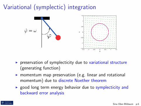
I preservation of symplecticity due to variational structure(generating function)

I momentum map preservation (e.g. linear and rotationalmomentum) due to discrete Noether theorem

I good long term energy behavior due to symplecticity andbackward error analysis


Motivation

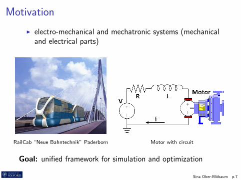
I electro-mechanical and mechatronic systems (mechanicaland electrical parts)

RailCab “Neue Bahntechnik” Paderborn Motor with circuit

Goal: unified framework for simulation and optimization


Motivation

Mechanical systems:

I variational integrators well established

I based on discrete variational principle in mechanics

Electrical systems:

+!

C1

C2L

R

UV

I variational principle required

I Lagrangian formulation withdegenerate symplectic form

I forces and constraints

I discrete variational scheme

Future goal: powerful unified variational scheme for thesimulation and optimization of electromechanical systems


Outline

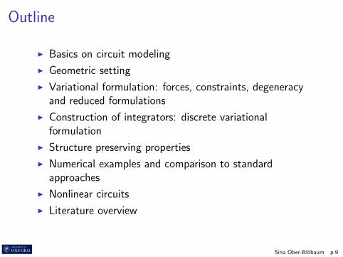
I Basics on circuit modeling

I Geometric setting

I Variational formulation: forces, constraints, degeneracyand reduced formulations

I Construction of integrators: discrete variationalformulation

I Structure preserving properties

I Numerical examples and comparison to standardapproaches

I Nonlinear circuits

I Literature overview


Basic notations

+!

C1

C2L

R

UV

device linear nonlinear

resistor iR = GuR iR = g(uR , t)

capacitor iC = C ddt uC iC = d

dt qC (uC , t)

inductor uL = L ddt iL uL = d

dtϕL(iL, t)

device independent controlled

voltage source uV = v(t) uV = v(uctrl , ictrl , t)current source iI = i(t) iI = i(uctrl , ictrl , t)

characteristic equations for basic elements


Energies in electric circuits

I magnetic energy stored in inductor

Emag(iL) =

∫ iL

0

ϕL(y) dy

I electrical energy stored in capacitor

Eel(qC ) =

∫ qC

0

uC (y) dy

linear circuit: ϕL(iL) = LiL and uC (qC ) = C−1qC

Emag(iL) =1

2Li2L , Eel(qC ) =

1

2C−1q2

C


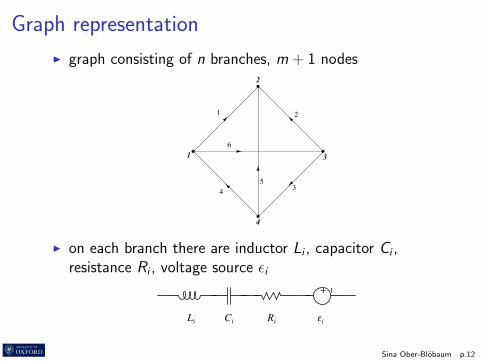
Graph representation

I graph consisting of n branches, m + 1 nodes

1 2

345

61

2

3

4

I on each branch there are inductor Li , capacitor Ci ,resistance Ri , voltage source εi

+ !

Li Ci Ri "i


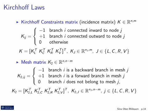
Kirchhoff Laws

Kirchhoff Current Law (KCL)

The sum of currents leading to and leaving from any node isequal to zero.

∑i = 0

Kirchhoff Voltage Law (KVL)

The sum of voltages along each mesh of the network is equalto zero.

∑u = 0


Kirchhoff Laws

I Kirchhoff Constraints matrix (incidence matrix) K ∈ Rn,m

Kij =

−1 branch i connected inward to node j+1 branch i connected outward to node j0 otherwise

K = [KTL KT

C KTR KT

V ]T , KJ ∈ RnJ ,m, J ∈ L,C ,R ,V

I Mesh matrix K2 ∈ Rn,n−m

K2,ij =

−1 branch i is a backward branch in mesh j+1 branch i is a forward branch in mesh j0 branch i does not belong to mesh j ,

K2 = [KT2,L K

T2,C KT

2,R KT2,V ]T , K2,J ∈ RnJ ,n−m, j ∈ L,C ,R ,V


Kirchhoff Laws

Kirchhoff Current Law (KCL)

The sum of currents leading to and leaving from any node isequal to zero.

∑i = 0 KT ·i(t) = 0

Kirchhoff Voltage Law (KVL)

The sum of voltages along each mesh of the network is equalto zero.

∑u = 0 KT

2 ·u(t) = 0

Tellegen’s theorem: im(K2) ⊥ im(K )


Geometric setting

configuration, tangent and cotangent space

I charge space Q, branch charge q ⊆ Rn

I current space TQ, branch currents (i =)v ∈ TqQ ⊆ Rn

I flux linkage space T ∗Q, flux linkages p ∈ T ∗qQ ⊆ Rn

constraint distribution and annihilator


Geometric setting






I constraint distribution

∆Q(q) = v ∈ TqQ | 〈w a, v〉 = 0, a = 1, . . . ,m ⊂ TqQ

I annihilator

∆0Q(q) = w ∈ T ∗qQ | 〈w , v〉 = 0 ∀v ∈ ∆Q(q) ⊂ T ∗qQ


Geometric setting






I constraint KCL space

∆Q(q) = v ∈ TqQ |KTv = 0 ⊂ TqQ

I constraint KVL space

∆0Q(q) = u ∈ T ∗qQ |KT

2 u = 0 ⊂ T ∗qQ


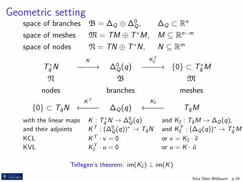
Geometric settingspace of branches B = ∆Q ⊕∆0

Q , ∆Q ⊂ Rn

space of meshes M = TM ⊕ T ∗M , M ⊆ Rn−m

space of nodes N = TN ⊕ T ∗N , N ⊆ Rm

T ∗qNK

−−−−→ ∆0Q(q)

KT2

−−−−→ 0 ⊂ T ∗qM

N B M

nodes branches meshes

0 ⊂ TqNKT

←−−−− ∆Q(q)K2

←−−−− TqM

with the linear maps K : T ∗qN → ∆0

Q(q) and K2 : TqM → ∆Q(q),

and their adjoints KT : (∆0Q(q))∗ → TqN and KT

2 : (∆Q(q))∗ → T ∗qM

KCL KT · v = 0 or v = K2 · vKVL KT

2 · u = 0 or u = K · u

Tellegen’s theorem: im(K2) ⊥ im(K )


Variational formulation

mechanical system electrical circuit (linear relations)

kinetic energy magnetic energy 12vTLv ∈ R

potential energy electrical energy 12qTCq ∈ R

friction dissipation R · v ∈ Rn

external force external sources E · u ∈ Rn

(non)holonomic constraints KCL KT · v = 0

withL = diag(L1, . . . , Ln), C = diag( 1

C1, . . . , 1

Cn),

R = diag(R1, . . . ,Rn), E = diag(ε1, . . . , εn)


Variational formulationI Lagrangian L(q, v) = 1

2vTLv − 1

2qTCq on TQ

I forces f = −R · v + E · u ∈ T ∗qQ

I distribution ∆Q(q) = v ∈ TqQ |KTv = 0 = null(KT )

1. dissipative and external forces (d’Alembert)

2. KCL constraints (constrained variations)

3. degenerate Lagrangian

I Legendre transformation FL(q, v) = (q, ∂L/∂v)

if∂2L∂v 2

= L is not invertible ⇒ degenerate system

I constraint flux linkage subspace

P = FL(∆Q) ⊂ T ∗Q,


Constrained variational formulationI Constrained Lagrange-d’Alembert-Pontryagin Principle on

TQ⊕

T ∗Q gives implicit Euler-Lagrange equations

[Yoshimura, Marsden 2006]

δ

∫ T

0

(L(q, v) + 〈p, q − v〉) dt +

∫ T

0

f ·δqdt = 0, δq ∈ ∆Q(q)



TQ⊕



δ

∫ T

0

(L(q, v) + 〈p, q − v〉) dt +

∫ T

0

f ·δqdt = 0, δq ∈ ∆Q(q)

see blackboard



TQ⊕



δ

∫ T

0

(L(q, v) + 〈p, q − v〉) dt +

∫ T

0

f ·δqdt = 0, δq ∈ ∆Q(q)

⇒

q = v charge-current relation

p = ∂L∂q

+ f + K · u KVL form u = K · u0 = ∂L

∂v− p flux relation (“primary constraints”)

0 = KT · v KCL

n + n + n + m equations

I differential-algebraic system

I differential variables q and p, algebraic variables v and u

I non-autonomous system due to external force f (t)

I no ode description for singular Lagrangian


Reduction

1. less redundant formulation

2. degeneracy of Lagrangian is cancelled for specific systems

3. physical meaning of reduced space: mesh space M withcoordinates (q, v , p), q, v , p ∈ Rn−m

T ∗qNK

−−−−→ ∆0Q(q)

KT2

−−−−→ 0 ⊂ T ∗qM

N B M


0 ⊂ TqNKT

←−−−− ∆Q(q)K2

←−−−− TqM


Reduction

1. less redundant formulation

2. degeneracy of Lagrangian is cancelled for specific systems

3. physical meaning of reduced space: mesh space M withcoordinates (q, v , p), q, v , p ∈ Rn−m

T ∗qNK

−−−−→ ∆0Q(q)

KT2

−−−−→ 0 ⊂ T ∗qM

N B M


0 ⊂ TqNKT

←−−−− ∆Q(q)K2

←−−−− TqM


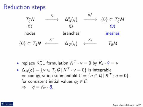
Reduction steps

T ∗qNK

−−−−→ ∆0Q(q)

KT2

−−−−→ 0 ⊂ T ∗qM

N B M


0 ⊂ TqNKT

←−−−− ∆Q(q)K2

←−−−− TqM

I replace KCL formulation KT · v = 0 by K2 · v = v

I ∆Q(q) = v ∈ TqQ |KT · v = 0 is integrable⇒ configuration submanifold C = q ∈ Q |KT · q = 0for consistent initial values q0 ∈ C⇒ q = K2 · q.


Reduction steps

T ∗qNK

−−−−→ ∆0Q(q)

KT2

−−−−→ 0 ⊂ T ∗qM

N B M


0 ⊂ TqNKT

←−−−− ∆Q(q)K2

←−−−− TqM

I constrained Lagrangian LM := K ∗2L : TM → R

LM(q, v) = L(K2q,K2v) =1

2vTKT

2 LK2v −1

2qTKT

2 CK2q

I reduced Legendre transformation FLM : TM → T ∗M

FLM(q, v) = (q, ∂LM/∂v) = (q,KT2 LK2v).

I reduced force f M(q, v , t) = KT2 f (K2q,K2v , t) in T ∗M

I reduced flux p = KT2 p in T ∗M


Reduced constrained variational formulationI reduced L-d’A-Pontryagin Principle on TM

⊕T ∗M

δ

∫ T

0

(LM(q, v) + 〈p, ˙q − v〉

)dt +

∫ T

0

f M · δqdt = 0

I implicit Euler-Lagrange equations on mesh space M

⇒

˙q = v

˙p =∂LM

∂q+ f KVL form KT

2 · u = 0

0 =∂LM

∂v− p with

∂LM

∂v= KT

2 LK2 · v

3 · (n −m) equationsI differential variables q and p, algebraic variable v

Is∂2LM

∂v 2= KT

2 LK2 invertible?


Cancellation of degeneracy by constraints

Cancellation of degeneracy

For linear LRCV circuits the system is non-degenerate, if thenumber of capacitors nC , resistors nR and voltage sources nVequals the number of independent constraints lX involving thecurrents through the capacitor, resistor and source branches,i.e., if

nC + nR + nV = lX

I Proof uses basic linear algebra arguments showing

1. null([KTC KT

R KTV ]) = 0

2. ⇒ null(KT2 LK2) = 0


Examples

L1

L2C1

C2

1

2

3 1

2

L1

C1 C2 C3

KTL =

(1 00 −1

), KT

C =

(0 −1−1 1

)KTL =

(10

), KT

C =

(−1 0 01 −1 −1

)null(KT

C ) = 0 null(KTC ) 6= 0

⇓ ⇓non-degenerate constrained Lagrangian degenerate constrained Lagrangian

I interpretation: Each fundamental loop has to contain atleast one inductor


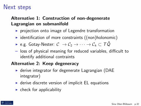
Next steps

Alternative 1: Construction of non-degenerateLagrangian on submanifold

I projection onto image of Legendre transformation

I identification of more constraints ((non)holonomic)

I e.g. Gotay-Nester: C → C2 → · · · → Ck ⊂ TQ

– loss of physical meaning for reduced variables, difficult toidentify additional contraints

Alternative 2: Keep degeneracy

I derive integrator for degenerate Lagrangian (DAEintegrator)

I derive discrete version of implicit EL equations

I check for applicability


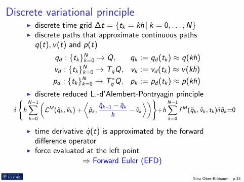
Discrete variational principleI discrete time grid ∆t = tk = kh | k = 0, . . . ,NI discrete paths that approximate continuous paths

q(t), v(t) and p(t)

qd : tkNk=0 → Q, qk := qd(tk) ≈ q(kh)

vd : tkNk=0 → TqQ, vk := vd(tk) ≈ v(kh)

pd : tkNk=0 → T ∗qQ, pk := pd(tk) ≈ p(kh)

I discrete reduced L.-d’Alembert-Pontryagin principle

δ

h

N−1∑k=0

(LM(qk , vk) +

⟨pk ,

qk+1 − qkh

− vk

⟩)+h

N−1∑k=0

f M(qk , vk , tk)δqk=0

I time derivative q(t) is approximated by the forwarddifference operator

I force evaluated at the left point⇒ Forward Euler (EFD)


Discrete variational principleI discrete time grid ∆t = tk = kh | k = 0, . . . ,NI discrete paths that approximate continuous paths

q(t), v(t) and p(t)

qd : tkNk=0 → Q, qk := qd(tk) ≈ q(kh)

vd : tkNk=0 → TqQ, vk := vd(tk) ≈ v(kh)

pd : tkNk=0 → T ∗qQ, pk := pd(tk) ≈ p(kh)

I discrete reduced L.-d’Alembert-Pontryagin principle

δ

h

N∑k=1

(LM(qk , vk) +

⟨pk ,

qk − qk−1

h− vk

⟩)+h

N∑k=1

f M(qk , vk , tk)δqk=0

I time derivative q(t) is approximated by the backwarddifference operator

I force evaluated at the right point

⇒ Backward Euler (EBD)


Discrete variation

I discrete variations δqk with δq0 = δqN = 0

I discrete variations δvk and δpk

⟨∂LM

∂v(q0, v0)− p0, δv0

⟩+

N−1∑k=1

[⟨∂LM

∂v(qk , vk)− pk , δvk

⟩+

⟨∂LM

∂q(qk , vk)− 1

h(pk − pk−1) + f M(qk , vk , tk), δqk

⟩⟨δpk−1,

qk − qk−1

h− vk−1

⟩]+

⟨δpN−1

qN − qN−1

h− vN−1

⟩= 0


Discrete reduced Euler-Lagrange equations

∂LM

∂v(q0, v0) = p0,

qN − qN−1

h= vN−1

∂LM

∂q(qk , vk)− 1

h(pk − pk−1) + f M(qk , vk , tk) = 0

qk − qk−1

h= vk−1

Forward Euler∂LM

∂v(qk , vk) = pk

k = 1, . . . ,N − 1

q1 − q0h

= v1,∂LM

∂v(q1, v1) = p1

∂LM

∂q(qk−1, vk−1)− 1

h(pk − pk−1) + f M(qk−1, vk−1, tk−1) = 0

qk − qk−1

h= vk

Backward Euler∂LM

∂v(qk , vk) = pk

k = 2, . . . ,N


Applicability

I apply e.g. Newton’s scheme to determinexk+1 = (qk+1, vk+1, pk+1) by solving 0 = F (xk , xk+1) forgiven xk = (qk , vk , pk)

I unique solutions for regular Jacobian of F w.r.t. xk+1

I applicability dependent on update rule

Example: EBD for linear circuit leads to the iteration scheme

I −hI 0

0 KT2 LK2 −I

0 0 I

︸︷︷︸

=A

qkvkpk

=

I 0 0

0 0 0

−hKT2 CK2 −hKT

2 diag(R)K2 I

qk−1

vk−1

pk−1

+

0

0

hKT2

us(tk−1)

A is invertible iff KT2 LK2 is regular


Applicability

I apply e.g. Newton’s scheme to determinexk+1 = (qk+1, vk+1, pk+1) by solving 0 = F (xk , xk+1) forgiven xk = (qk , vk , pk)

I unique solutions for regular Jacobian of F w.r.t. xk+1

I applicability dependent on update rule

Example: EFD for linear circuit leads to the iteration scheme

I 0 0

0 KT2 LK2 −I

hKT2 CK2 hKT

2 diag(R)K2 I

︸︷︷︸

=A

qkvkpk

=

I hI 0

0 0 0

0 0 I

qk−1

vk−1

pk−1

+

0

0

hKT2

us(tk )

A is invertible iff KT2 (L+hR)K2 is regular


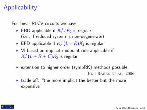
Applicability

For linear RLCV circuits we have

I EBD applicable if KT2 LK2 is regular

(i.e., if reduced system is non-degenerate)

I EFD applicable if KT2 (L + R)K2 is regular

I VI based on implicit midpoint rule applicable ifKT

2 (L + R + C )K2 is regular

I extension to higher order (sympRK) methods possible[Bou-Rabee et al. 2006]

I trade off: “the more implicit the better but the moreexpensive”


Structure preservation – symplecticity

I symlecticity: conservation of symplectic formΩ = dqi ∧ dpi

(F t)∗Ω = Ω ∀tI conformal symlecticity (in presence of uniform dissipative

forces fL = c · p, c ∈ R):

(F t)∗Ω = exp (ct)Ω ∀t

I variational integrator preserves the symplectic form, orthe rate of decay of the symplectic form, respectively

I leads to good long-term energy behavior of variationalintegrators

e.g. Hairer, Lubich 2004


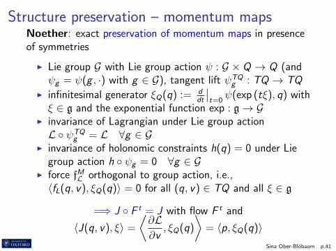
Structure preservation – momentum mapsNoether: exact preservation of momentum maps in presenceof symmetries

I Lie group G with Lie group action ψ : G × Q → Q (andψg = ψ(g , ·) with g ∈ G), tangent lift ψTQ

g : TQ → TQI infinitesimal generator ξQ(q) := d

dt

∣∣t=0

ψ(exp (tξ), q) withξ ∈ g and the exponential function exp : g→ G

I invariance of Lagrangian under Lie group actionL ψTQ

g = L ∀g ∈ GI invariance of holonomic constraints h(q) = 0 under Lie

group action h ψg = 0 ∀g ∈ GI force fML orthogonal to group action, i.e.,〈fL(q, v), ξQ(q)〉 = 0 for all (q, v) ∈ TQ and all ξ ∈ g

=⇒ J F t = J with flow F t and

〈J(q, v), ξ〉 =

⟨∂L∂v

, ξQ(q)

⟩= 〈p, ξQ(q)〉


Structure preservation – momentum maps

I Examples from mechanics

G = R temporal ⇒ energy

G = R3 translational ⇒ linear momentum

G = SO(3) rotational ⇒ angular momentum

I variational integrator preserves the invariance property ifthe discrete Lagrangian has the same symmetry

What are momentum maps for electric circuits?Which symmetries can we expect?


Momentum maps for electric circuitsI Lagrangian L(q, v) = 1

2vTLv − 1

2qTCq

I force f = −Rv + Eu, KCL KTv = 0

Invariance of Lagrangian

The Lagrangian of the unreduced system is invariant under thetranslation of qL.

Proof:Let G = RnL , ΦTQ(g , (q, v)) = (qL + g , qC , qR , qV , vL, vC , vR , vV )

LΦTQg (q, v) =

1

2

vLvCvRvV

T

L

vLvCvRvV

− 1

2

qL + gqCqRqV

T

C

qL + gqCqRqV

= 1

2vTLv − 1

2qTCq = L(q, v) since C = diag

(1C1, . . . , 1

Cn

)with the first nL diagonal elements being zero.


Momentum maps for electric circuitsI Lagrangian L(q, v) = 1

2vTLv − 1

2qTCq

I force f = −Rv + Eu, KCL KTv = 0

Orthogonality of external force

The external force f is orthogonal to the action of the groupG = RnL being translations of qL.

Proof: Let ξ ∈ g = RnL . For Φg (q) = (qL + g , qC , qR , qV ) we compute

ξQ(q) =d

dt

∣∣∣∣t=0

Φexp tξ(q) =d

dt

∣∣∣∣t=0

(qL+exp tξ, qC , qR , qV ) = (ξ, 0, 0, 0).

Thus, we have

〈fL, ξQ(q)〉 = 〈−Rv + Eu, ξQ(q)〉 = 0

since R and E have zero entries in the first nL lines and columns.


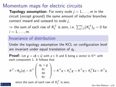
Momentum maps for electric circuitsTopology assumption: For every node j = 1, . . . ,m in thecircuit (except ground) the same amount of inductor branchesconnect inward and outward to node j .

⇒ the sum of each row of KTL is zero, i.e.

∑nLj=1(KT

L )ij = 0 fori = 1, . . . ,m.

Invariance of distribution

Under the topology assumption the KCL on configuration levelare invariant under equal translation of qL.

Proof: Let g = a1 ∈ G with a ∈ R and 1 being a vector in RnL witheach component 1. It follows that

KT Φg (q) = KT

qL + gqCqRqV

= KTq + KTL g = KTq + KT

L 1a = KTq

since the sum of each row of KTL is zero.


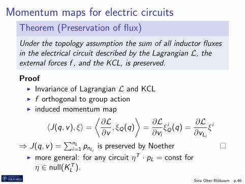
Momentum maps for electric circuits

Theorem (Preservation of flux)

Under the topology assumption the sum of all inductor fluxesin the electrical circuit described by the Lagrangian L, theexternal forces f , and the KCL, is preserved.

ProofI Invariance of Lagrangian L and KCLI f orthogonal to group actionI induced momentum map

〈J(q, v), ξ〉 =

⟨∂L∂v

, ξQ(q)

⟩=∂L∂vi

ξiQ(q) =∂L∂vLi

ξi

⇒ J(q, v) =∑nL

i=1 pnLi is preserved by Noether

I more general: for any circuit ηT · pL = const forη ∈ null(KT

L ).


Example: LC transmission line

1 2L1 L2 L3

C1 C2

0 10 20 30 40 50 60 70 80 90−1

−0.5

0

0.5

1

1.5

2

time

flux

pL1

pL2pL3

pL1+pL2+pL3

K =

−1 01 −10 11 00 1

KL =

−1 01 −10 1

KC =

(1 00 1

)nL∑j=1

(KTL )ij = 0, i = 1, 2

⇒ pL1 + pL2 + pL3 = constSina Ober-Blobaum p.47

Structure preservation – what else?

Preservation of frequency spectrum

I consider the example of the 1D harmonic oscillator

I define one-step update scheme as

(qk+1, pk+1)T = A · (qk , pk)T = QVQ−1 · (qk , pk)T

with A having linearly independent eigenvectors λ1, λ2and being diagonalizable with V = diag(λ1, λ2)

I with the coordinate transformation(xk , yk)T = Q−1 · (qk , pk)T we obtain

(xk+1, yk+1)T = V · (xk , yk)T

i.e., xk+1 = λ1xk and yk+1 = λ2yk


Structure preservation – frequency spectrumWe show

1. A has two eigenvalues of norm 1 iff scheme is symplectic

2. methods defined by matrices with norm 1 eigenvaluespreserve frequeny spectrum defined on different timespans

Proof of 2.

I discrete inverse Fourier transformationxk = 1

N

∑Nn=1 xn exp

(2πiN kn

), k = 1, . . . ,N

I Consider a sequence of discrete points XkNk=1 that is shifted byone time step such that Xk = xk+1 = λ1xk , k = 1, . . . ,N

I discrete inverse Fourier transformationXk = 1

N

∑Nn=1 λ1xn exp

(2πiN kn

), k = 1, . . . ,N, i.e., Xn = λ1xn

I by definition of the frequency spectrum, we haveX ∗n Xn = x∗nλ

∗1λ1xn = x∗n |λ1|2xn = x∗n xn

⇒ “preservation of the frequency spectrum”


Standard methods in circuit theory

I Circuit simulator SPICE (Simulation Program withIntegrated Circuit Emphasis)

Electronics Research Laboratory of the University

of California, Berkeley

I Modeling: Modified Node Analysis (MNA)

I Simulation: Backward Differentiation Formulas (BDF)methods


Modified Nodal Analysis (MNA) (charge-flux)

1. Apply KCL to every node except ground

2. Insert representation for the branch current of resistors,capacitors and current sources

3. Add representation for inductors and voltage sourcesexplicitely to the system

(KCL) KTC qC (KC u, t) + KT

R g(KR u, t) + KTL vL + KT

V vV

+KTI vI (Ku, qC (KC u, t), vL, vV , t) = 0

(inductors) pL(vL, t)− KLu = 0

(voltage sources) uV (Ku, qC (KCu, t), vL, vV , t)− KV u = 0

I inductor current vL, capacitor charge qC , inductor flux pLI node voltage u, voltage source current vV , conductance g

I controlled current and voltage source vI and uV


Numerical integration schemesI DAE system A[d(x(t), t)]′ + b(x(t), t) = 0 with

x = [u, vL, vv ]T and d(x , t) = [qC (KC u, t), pL(vL, t)]T

I conventional approach: Implicit linear multi-step formulas

k∑i=0

αid(xn+1−i , tn+1−i) = hk∑

i=0

βid′n+1−i

I BDF method: β1 = · · · = βk = 0, α0 = 1k β0 α1 α2 scheme1 1 −1 d(xn+1)− d(xn) = hd ′n+1 (implicit Euler)

2 23−4

313

d(xn+1)− 43d(xn) + 1

3d(xn−1) = h 2

3d ′n+1⊕

low computational cost (1 function evaluation per step)compared to RK methods

BUT non-symplectic (Tang 1993)


Example computations

Comparison of different solutions

I exact solution (exact)

I variational integrator of second order (VI)

I variational integrator of first order (EBD)

I variational integrator of first order (EFD)

I Runge Kutta of order 4 (RK)

I BDF method of order 2 applied to MNA system (MNABDF)

(fixed time-stepping for all methods)


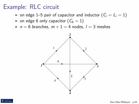
Example: RLC circuitI on edge 1–5 pair of capacitor and inductor (Ci = Li = 1)I on edge 6 only capacitor (C6 = 1)I n = 6 branches, m + 1 = 4 nodes, l = 3 meshes

1 2

345

61

2

3

4


LC circuit (no resistors) with step size h = 0.1

0 5 10 15 20 25

−1

−0.5

0

0.5

1

time

curre

nt o

n br

anch

1

0 5 10 15 20 25

−1

−0.5

0

0.5

1

time

curre

nt o

n br

anch

2

current branch 1 current branch 2

0 5 10 15 20 25

−1

−0.8

−0.6

−0.4

−0.2

0

0.2

0.4

0.6

0.8

1

time

curre

nt o

n br

anch

3

0 5 10 15 20 25

1.42

1.44

1.46

1.48

1.5

1.52

1.54

1.56

1.58

1.6

time

ener

gy

exactVIVI EBDVI EFDRK4MNA BDF

current branch 3 energy behavior


LC circuit (no resistors) with step size h = 0.4

180 182 184 186 188 190 192 194 196 198 200−1.5

−1

−0.5

0

0.5

1

1.5

time

curre

nt o

n br

anch

1


180 182 184 186 188 190 192 194 196 198 200−1.5

−1

−0.5

0

0.5

1

1.5

time

curre

nt o

n br

anch

2



180 182 184 186 188 190 192 194 196 198 200−1.5

−1

−0.5

0

0.5

1

1.5

time

curre

nt o

n br

anch

3


0 100 200 300 400 500 600 700

0.2

0.4

0.6

0.8

1

1.2

1.4

1.6

1.8

2

time

ener

gy




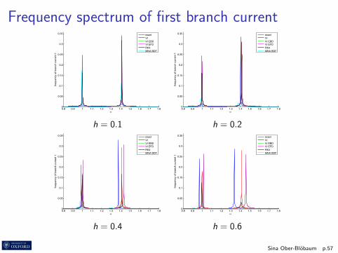
Frequency spectrum of first branch current

0.8 0.9 1 1.1 1.2 1.3 1.4 1.5 1.6 1.7 1.80

0.05

0.1

0.15

0.2

0.25

0.3

0.35

!

frequ

ency

of b

ranc

h cu

rrent

1


0.8 0.9 1 1.1 1.2 1.3 1.4 1.5 1.6 1.7 1.80

0.05

0.1

0.15

0.2

0.25

0.3

0.35

!

frequ

ency

of b

ranc

h cu

rrent

1


h = 0.1 h = 0.2

0.8 0.9 1 1.1 1.2 1.3 1.4 1.5 1.6 1.7 1.80

0.05

0.1

0.15

0.2

0.25

0.3

0.35

!

frequ

ency

of b

ranc

h cu

rrent

1


0.8 0.9 1 1.1 1.2 1.3 1.4 1.5 1.6 1.7 1.80

0.05

0.1

0.15

0.2

0.25

0.3

0.35

!

frequ

ency

of b

ranc

h cu

rrent

1


h = 0.4 h = 0.6


Current of first branch of LC circuit (no resistors)

0 500 1000 1500 2000 2500 3000

−1

−0.5

0

0.5

1

time

curre

nt o

n br

anch

1

exactVIRK4MNA BDF

0 500 1000 1500 2000 2500 3000

−1

−0.5

0

0.5

1

time

curre

nt o

n br

anch

1

exactVIRK4MNA BDF

h = 0.1 h = 0.2

0 500 1000 1500 2000 2500 3000

−1

−0.5

0

0.5

1

time

curre

nt o

n br

anch

1

exactVIRK4MNA BDF

0 500 1000 1500 2000 2500 3000

−1

−0.5

0

0.5

1

time

curre

nt o

n br

anch

1

exactVIRK4MNA BDF

h = 0.4 h = 0.6


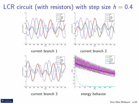
LCR circuit (with resistors) with step size h = 0.4

180 182 184 186 188 190 192 194 196 198 200−1.5

−1

−0.5

0

0.5

1

1.5

time

curre

nt o

n br

anch

1


180 182 184 186 188 190 192 194 196 198 200−1.5

−1

−0.5

0

0.5

1

1.5

time

curre

nt o

n br

anch

2



180 182 184 186 188 190 192 194 196 198 200−1.5

−1

−0.5

0

0.5

1

1.5

time

curre

nt o

n br

anch

3


0 50 100 150 200 250 300 350

0.2

0.4

0.6

0.8

1

1.2

1.4

1.6

1.8

time

ener

gy




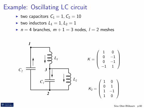
Example: Oscillating LC circuitI two capacitors C1 = 1,C2 = 10

I two inductors L1 = 1, L2 = 1

I n = 4 branches, m + 1 = 3 nodes, l = 2 meshes

L1

L2C1

C2

1

2

3

K =

1 00 −10 −1−1 1

K2 =

1 00 11 −11 0


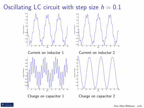
Oscillating LC circuit with step size h = 0.1

0 10 20 30 40 50 60 70 80 90 100

−0.2

−0.15

−0.1

−0.05

0

0.05

0.1

0.15

0.2

0.25

time

curre

nt o

n br

anch

1

0 10 20 30 40 50 60 70 80 90 100−0.25

−0.2

−0.15

−0.1

−0.05

0

0.05

0.1

0.15

0.2

0.25

time

curre

nt o

n br

anch

2

Current on inductor 1 Current on inductor 2

0 10 20 30 40 50 60 70 80 90 100

−0.08

−0.06

−0.04

−0.02

0

0.02

0.04

0.06

0.08

time

char

ge o

n br

anch

3

0 10 20 30 40 50 60 70 80 90 100

−0.8

−0.6

−0.4

−0.2

0

0.2

0.4

0.6

0.8

1

time

char

ge o

n br

anch

4

Charge on capacitor 1 Charge on capacitor 2


Energy of oscillating LC circuit

0 500 1000 1500 2000 2500 30000.0486

0.0488

0.049

0.0492

0.0494

0.0496

0.0498

0.05

0.0502

0.0504

0.0506

time

ener

gy


0 500 1000 1500 2000 2500 3000

0.0475

0.048

0.0485

0.049

0.0495

0.05

0.0505

0.051

time

ener

gy


h = 0.1 h = 0.2

0 500 1000 1500 2000 2500 3000

0.04

0.042

0.044

0.046

0.048

0.05

0.052

time

ener

gy


0 500 1000 1500 2000 2500 3000

0.025

0.03

0.035

0.04

0.045

0.05

time

ener

gy


h = 0.4 h = 0.6


Charge on capacitor 1 of LC circuit (h = 0.6)

0 500 1000 1500 2000 2500 3000−0.1

−0.08

−0.06

−0.04

−0.02

0

0.02

0.04

0.06

0.08

0.1

time

char

ge o

n br

anch

3


0 5 10 15 20 25 30 35 40 45 50−0.1

−0.08

−0.06

−0.04

−0.02

0

0.02

0.04

0.06

0.08

0.1

time

char

ge o

n br

anch

3


t ∈ [0, 3000] t ∈ [0, 50]

300 305 310 315 320 325 330 335 340 345 350−0.1

−0.08

−0.06

−0.04

−0.02

0

0.02

0.04

0.06

0.08

0.1

time

char

ge o

n br

anch

3


2500 2505 2510 2515 2520 2525 2530 2535 2540 2545 2550−0.1

−0.08

−0.06

−0.04

−0.02

0

0.02

0.04

0.06

0.08

0.1

time

char

ge o

n br

anch

3


t ∈ [300, 350] t ∈ [2500, 2550]


Frequency spectrum of charge on capacitor 1

1.3 1.35 1.4 1.45 1.5 1.550

0.005

0.01

0.015

0.02

0.025

0.03

!

frequ

ency

of b

ranc

h ch

arge

3


1.3 1.35 1.4 1.45 1.5 1.550

0.005

0.01

0.015

0.02

0.025

0.03

!

frequ

ency

of b

ranc

h ch

arge

3


h = 0.1 h = 0.2

1.3 1.35 1.4 1.45 1.5 1.550

0.005

0.01

0.015

0.02

0.025

0.03

!

frequ

ency

of b

ranc

h ch

arge

3


1.3 1.35 1.4 1.45 1.5 1.550

0.005

0.01

0.015

0.02

0.025

0.03

!

frequ

ency

of b

ranc

h ch

arge

3


h = 0.4 h = 0.6


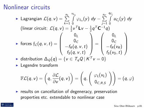
Nonlinear circuits

I Lagrangian L(q, v) =nL∑k=1

vLk∫0

ϕLk (y) dy −nC∑j=1

qCj∫0

uCj(y) dy

(linear circuit: L(q, v) = 12vTLv − 1

2qTC−1q)

I forces fL(q, v , t) =

0L

0C

−fR(q, v , t)fS(q, v , t)

=

0L

0C

−fR(vR)fS(vS , t)

I distribution ∆Q(q) = v ∈ TqQ |KTv = 0I Legendre transform

FL(q, v) =

(q,∂L∂v

(q, v)

)=

(q,

(ϕL(vL)

0C ,R,S

))= (q, ϕ)

I results on cancellation of degeneracy, preservationproperties etc. extendable to nonlinear case


Nonlinear LCR circuitLagrangian:

L(qC , vL) =c

2v2L1

+d

2log((tan(vL2/d))2+1)

−sgn(qC1)a

3q3C1− 1

2bq2C2

force: fR(vR) = ev3R

(a = 0.002, b =1

30, c = 30, d = 1, e = 5000)

0 100 200 300 400 500 600 700 8000.1

0.2

0.3

0.4

0.5

0.6

0.7

0.8

time

energ

y

VI EFD

VI EBD

VI MPR

RK4

ODE45

exact

0 100 200 300 400 500 600 700 8000

0.1

0.2

0.3

0.4

0.5

0.6

0.7

0.8

time

energ

y

VI EFD

VI EBD

VI MPR

RK4

ODE45

energy, no resistor (h = 0.08) energy with resistor (h = 0.08)


Conclusions

I variational approach for circuit modeling (degenerateLagrangian, dissipative and external forces, KCLconstraints)

I reduced variational approach on mesh space (cancelsdegeneracy for some cases, reduced system)

I discrete variational approach provides structure-preservingintegrator

I preservation of momentum mapsI preservation of frequency spectrumI good energy behavior

I variational integrators are convenient tools for thesimulation of electric and electromechanical systems


Literature overviewVariational inegrators for electric circuits

I Ober-Blobaum, Tao, Cheng, Owhadi, Marsden (2013):linear circuits

I Ober-Blobaum, Lindhorst (2014): nonlinear circuits

Lagrangian / Hamiltonian modeling of circuits

I MacFarlane (1967): tree structures (capacitor charges orinductor fluxes as generalized coordinates)

I Chua, McPherson (1973): mixed set of coordinates

I Maisser et al. (1995): Lagrangian modeling ofelectromechanical systems

Degenerate Lagrangian / Hamiltonian

I Dirac, Bergmann (1956): construction of submanifolds

I Gotay, Nester (1979): Lagrangian viewpoint

I van der Schaft (1995): implicit Hamiltonian systems

I Yoshimura, Marsden (2006): implicit Lagrangian systems


Documents

Variational integrators for electric and nonsmooth systems · Variational integrators for electric and nonsmooth systems ... Variational integrators for electric circuits Ober-Bl