193

Chapter 5

Generalized Variational Integrators

Abstract

In this chapter, we introduce generalized Galerkin variational integrators, which are a

natural generalization of discrete variational mechanics, whereby the discrete action,

as opposed to the discrete Lagrangian, is the fundamental object. This is achieved

by approximating the action integral with appropriate choices of a finite-dimensional

function space that approximate sections of the configuration bundle and numeri-

cal quadrature to approximate the integral. We discuss how this general framework

allows us to recover higher-order Galerkin variational integrators, asynchronous vari-

ational integrators, and symplectic-energy-momentum integrators. In addition, we

will consider function spaces that are not parameterized by field values evaluated at

nodal points, which allows the construction of Lie group, multiscale, and pseudospec-

tral variational integrators. The construction of pseudospectral variational integrators

is illustrated by applying it to the (linear) Schrodinger equation. G-invariant discrete

Lagrangians are constructed in the context of Lie group methods through the use of

natural charts and interpolation at the level of the Lie algebra. The reduction of these

G-invariant Lagrangians yield a higher-order analogue of discrete Euler–Poincare re-

duction. By considering nonlinear approximation spaces, spatio-temporally adaptive

variational integrators can be introduced as well.

5.1 Introduction

We will review some of the previous work on discrete mechanics and their multisymplectic gener-

alizations (see, for example, Marsden et al. [1998, 2001]), before introducing a general formulation

194

of discrete mechanics that recovers higher-order variational integrators (see, for example, Marsden

and West [2001]), asynchronous variational integrators (see, for example, Lew et al. [2003]), as well

symplectic-energy-momentum integrators (see, for example, Kane et al. [1999]).

While discrete variational integrators exhibit desirable properties such as symplecticity, momen-

tum preservation, and good energy behavior, it does not address other important issues in numerical

analysis, such as adaptivity and approximability. Generalized variational integrators are introduced

with a view towards addressing such issues in the context of discrete variational mechanics.

By formulating the construction of a generalized variational integrator in terms of the choice of

a finite-dimensional function space and a numerical quadrature scheme, we are able to draw upon

the extensive literature on approximation theory and numerical quadrature to construct variational

schemes that are appropriate for a larger class of problems. Within this framework, we will introduce

multiscale, spatio-temporally adaptive, Lie group, and pseudospectral variational integrators.

5.1.1 Standard Formulation of Discrete Mechanics

The standard formulation of discrete variational mechanics (see, for example, Marsden and West

[2001]) is to consider the discrete Hamilton’s principle,

δSd = 0,

where the discrete action sum, Sd : Qn+1 → R, is given by

Sd(q0, q1, . . . , qn) =n−1∑i=0

Ld(qi, qi+1).

The discrete Lagrangian, Ld : Q×Q→ R, is a generating function of the symplectic flow, and is

an approximation to the exact discrete Lagrangian,

Lexactd (q0, q1) =

∫ h

0

L(q01(t), q01(t))dt,

where q01(0) = q0, q01(h) = q1, and q01 satisfies the Euler–Lagrange equation in the time interval

(0, h). The exact discrete Lagrangian is related to the Jacobi solution of the Hamilton–Jacobi

equation. The discrete variational principle then yields the discrete Euler–Lagrange (DEL)

equation,

D2Ld(q0, q1) +D1Ld(q1, q2) = 0,

which yields an implicit update map (q0, q1) 7→ (q1, q2) that is valid for initial conditions (q0, q1)

that as sufficiently close to the diagonal of Q×Q.

195

5.1.2 Multisymplectic Geometry

The generalization of the variational principle to the setting of partial differential equations involves

a multisymplectic formulation (see, for example, Marsden et al. [1998, 2001]). Here, the base space

X consists of the independent variables, which are denoted by (x0, . . . , xn), where x0 is time, and

x1, . . . , xn are space variables.

The independent or field variables, denoted (q1, . . . , qm), form a fiber over each space-time base-

point. The set of independent variables, together with the field variables over them, form a fiber

bundle, π : Y → X , referred to as the configuration bundle. The configuration of the system is

specified by giving the field values at each space-time point. More precisely, this can be represented

as a section of Y over X , which is a continuous map q : X → Y , such that π q = 1X . This means

that for every x ∈ X , q(x) is in the fiber over x, which is π−1(x).

In the case of ordinary differential equations, the Lagrangian is dependent on the position vari-

able, and its time derivative, and the action integral is obtained by integrating the Lagrangian in

time. In the multisymplectic case, the Lagrangian density is dependent on the field variables, and

the derivatives of the field variables with respect to the space-time variables, and the action integral

is obtained by integrating the Lagrangian density over a region of space-time.

The analogue of the tangent bundle TQ in the multisymplectic setting is referred to as the first

jet bundle J1Y , which consists of the configuration bundle Y , together with the first derivatives of

the field variables with respect to independent variables. We denote these as,

vij = qi,j =∂qi

∂xj,

for i = 1, . . . ,m, and j = 0, . . . , n.

We can think of J1Y as a fiber bundle over X . Given a section q : X → Y , we obtain its first

jet extension, j1q : X → J1Y , that is given by

j1q(x0, . . . , xn) =(x0, . . . , xn, q1, . . . , qm, q1,1, . . . , q

m,n

),

which is a section of the fiber bundle J1Y over X .

The Lagrangian density is a map L : J1Y → Ωn+1(X ), and the action integral is given by

S(q) =∫XL(j1q),

and then Hamilton’s principle states that

δS = 0.

196

We will see in the next subsection how this allows us to construct multisymplectic variational inte-

grators.

5.1.3 Multisymplectic Variational Integrator

We introduce a multisymplectic variational integrator through the use of a simple but illustrative

example. We consider a tensor product discretization of (1 + 1)-space-time, given by

•

•

•

•

•

•

•

•

•

xi−1 xi xi+1

tj−1

tj

tj+1

∆t

∆x

and tensor product shape functions given by

ϕi,j(x, t) =

xi xi+1

1

//

OO

????

????

?

⊗

tj tj+1

1

//

OO

????

????

?

We construct the discrete Lagrangian as follows,

Ld(qi,j , qi+1,j , qi,j+1, qi+1,j+1) =∫

[xi,xi+1]

∫[tj ,tj+1]

L(j1(∑i+1

a=i

∑j+1

b=jqa,bϕa,b

)),

where qi,j ' q(i∆x, j∆t).

Consider a variation that varies the value of qi,j , and leaves the other degrees of freedom fixed,

then we obtain the following discrete Euler–Lagrange equation,

D1Ld(qi,j , qi+1,j , qi,j+1, qi+1,j+1)+D2Ld(qi−1,j , qi,j , qi−1,j+1, qi,j+1)

+D3Ld(qi,j−1, qi+1,j−1, qi,j , qi+1,j)

+D4Ld(qi−1,j−1, qi,j−1, qi−1,j , qi,j) = 0 ,

197

In general, when we take variations in a degree of freedom, we will have a discrete Euler–Lagrange

equation that involves all terms in the discrete action sum that are associated with regions in space-

time that overlap with the support of the shape function associated with that degree of freedom.

5.2 Generalized Galerkin Variational Integrators

There are a few essential observations that go into constructing a general framework that en-

compasses the prior work on variational integrators, asynchronous variational integrators, and

symplectic-energy-momentum integrators, while yielding generalizations that allow the construction

of multiscale, spatio-temporally adaptive, Lie group, and pseudospectral variational integrators.

The first is that a generalized Galerkin variational integrator involves the choice of a finite-

dimensional function space that discretizes a section of the configuration bundle, and the second is

that we approximate the action integral though a numerical quadrature scheme to yield a discrete

action sum. The discrete variational equations we obtain from this discrete variational principle are

simply the Karush–Kuhn–Tucker (KKT) conditions (see, for example, Nocedal and Wright [1999])

with respect to the degrees of freedom that generate the finite-dimensional function space.

To recap, the choices which are made in discretizing a variational problem are:

1. A finite-dimensional function space to represent sections of the configuration bundle.

2. A numerical quadrature scheme to evaluate the action integral.

Given these two choices, we obtain an expression for the discrete action in terms of the degrees of

freedom, and the KKT conditions for the discrete action to be stationary with respect to variations

in the degrees of freedom yield the generalized discrete Euler–Lagrange equations.

Current variational integrators are based on piecewise polynomial interpolation, with function

spaces that are parameterized by the value of the field variables at nodal points, and a set of

internal points. By relaxing the condition that the interpolation is piecewise, we will be able to

consider pseudospectral discretizations, and by relaxing the condition that the parameterization is

in terms of field values, we will be able to consider Lie group variational integrators. By considering

shape functions motivated by multiscale finite elements (see, for example, Hou and Wu [1999];

Efendiev et al. [2000]; Chen and Hou [2003]), we will obtain multiscale variational integrators. And

by generalizing the approach used in symplectic-energy-momentum integrators, and considering

nonlinear approximation spaces (see, for example, DeVore [1998]), we will be able to introduce

spatio-temporally adaptive variational integrators.

As we will see, there is nothing canonical about the form of the discrete Euler–Lagrange equations,

or the notion that the discrete Lagrangian is a map Ld : Q×Q→ R. These expressions arise because

198

of the finite-dimensional function space which has been chosen.

5.2.1 Special Cases of Generalized Galerkin Variational Integrators

In this subsection, we will show how higher-order Galerkin variational integrators, multisymplectic

variational integrators, and symplectic-energy-momentum integrators are all special cases of gener-

alized Galerkin variational integrators.

Higher-Order Galerkin Variational Integrators. In the case of higher-order Galerkin vari-

ational integrators, we have chosen a piecewise interpolation for each time interval [0, h], that is

parameterized by control points q10 , . . . qs0, corresponding to the value of the curve at a set of control

times 0 = d0 < d1 < . . . < ds−1 < ds = 1. The interpolation within each interval [0, h] is given by

the unique degree s polynomial qd(t; qν0 , h), such that qd(dνh) = gν0 , for ν = 0, . . . , s.

Q

t0 d1h d2h ds−2h ds−1h h

•

•

•q10

..... ...............•

••qs−10

q00q20

qs−20

qs0

//

OO

Figure 5.1: Polynomial interpolation used in higher-order Galerkin variational integrators.

By an appropriate choice of quadrature scheme, we can break up the action integral into pieces,

which we denote by

Sid(qνi ) ≈∫ h

0

L(qd(t; qνi , h), qd(t; qνi , h))dt.

If we further require that the piecewise defined curve is continuous at the node points, we obtain

the following augmented discrete action,

Sd(qνi i=0,...,N−1

ν=0,...,s

)=N−1∑i=0

Sid (qνi sν=0)−N−2∑i=0

λi(qsi − q0i+1).

The discrete action is stationary when

∂Sid∂qsi

(qνi ) = λi,

199

∂Sid∂q0i+1

(qνi+1) = −λi,

∂Sid∂qji

(qνi ) = 0.

We can identify the pieces of the discrete action with the discrete Lagrangian, Ld : Q×Q→ R, by

setting

Ld(qi, qi+1) = Sid(qνi ), (5.2.1)

where, q0i = qi, qsi = qi+1, and the other qji ’s are defined implicitly by the system of equations

∂Sid∂qji

(qνi ) = 0, (5.2.2)

for ν = 1, . . . , s− 1. Once we have made this identification, we have that

−D1Ld(qi+1, qi+2) = −Si+1d

∂q0i+1

(qνi+1)

= λi

=∂Sid∂qsi

(qνi )

= D2Ld(qi, qi+1),

from which we recover the discrete Euler–Lagrange equation,

D1Ld(qi+1, qi+2) +D2Ld(qi, qi+1) = 0.

The DEL equations, together with the definition of the discrete Lagrangian, given in Equations 5.2.1

and 5.2.2, yield a higher-order Galerkin variational integrator. As we have shown, it is only because

the interpolation was piecewise that we were able to decompose the equations into a DEL equation,

and a set of equations that define the discrete Lagrangian in terms of conditions on the internal

control points.

Multisymplectic Variational Integrators. Recall the example of a multisymplectic variational

integrator we introduced in §5.1.3, where we used tensor product linear shape functions with localized

supports to discretize the configuration bundle. The discrete action is then given by

Sd(qa,ba=0,...,M−1

b=0,...,N−1

)=∫

[x0,xM ]

∫[t0,tN ]

L(j1( N∑a=0

N∑b=0

qa,bϕa,b

))

200

=M−1∑i=0

N−1∑j=0

∫[xi,xi+1]

∫[tj ,tj+1]

L(j1( N∑a=0

N∑b=0

qa,bϕa,b

))

=M−1∑i=0

N−1∑j=0

∫[xi,xi+1]

∫[tj ,tj+1]

L(j1( i+1∑a=i

j+1∑b=j

qa,bϕa,b

)),

where we first decomposed the integral into pieces, and then used the local support of the shape

functions to simplify the inner sums over qa,bϕa,b. As before, it is due to the local support of the

shape functions that we can express the discrete action as

Sd =M−1∑i=0

N−1∑j=0

Ld(qi,j , qi+1,j , qi,j+1, qi+1,j+1),

where

Ld(qi,j , qi+1,j , qi,j+1, qi+1,j+1) =∫

[xi,xi+1]

∫[tj ,tj+1]

L(j1(∑i+1

a=i

∑j+1

b=jqa,bϕa,b

)),

This localized support is also the reason why the discrete Euler–Lagrange equation in this case

consists of four terms, since to each degree of freedom, there are four other degrees of freedom that

have shape functions with overlapping support. In the case of ordinary differential equations, this

was two. In general, for tensor product meshes of (n + 1)-space-times, with tent function shape

functions, the number of terms in the discrete Euler–Lagrange equation will be 2n+1. In contrast,

for pseudospectral variational integrators with m spatial degrees of freedom per time level, and k

degrees of freedom per piecewise polynomial in time, each of the m(k − 1) discrete Euler–Lagrange

equations will involve m(k − 1) terms.

This is simply a reflection of the fact that shape functions with compact support yield schemes

with banded matrix structure, whereas pseudospectral and spectral methods tend to yield fuller

matrices. The payoff in using pseudospectral and spectral methods for problems with smooth or an-

alytic solutions is due to the approximation theoretic property that these solutions are approximated

at an exponential rate of accuracy by spectral expansions.

Symplectic-Energy-Momentum Integrators. In the case of symplectic-energy-momentum in-

tegrators, the degrees of freedom involve both the base variables and the field variables. We will

first derive a second-order symplectic-energy momentum integrator, and in the next section, we will

derive a higher-order generalization. We choose a piecewise linear interpolation for our configura-

tion bundle. Each piece is parameterized by the endpoint values of the field variable q0i , q1i , and the

endpoint times h0i , h

1i , and we approximate the action integral using the midpoint rule. To ensure

continuity, we require that, q1i = q0i+1, and h1i = h0

i+1.

201

Remark 5.1. The approach of allowing each piecewise defined curve to float around freely, and

imposing the continuity conditions using Lagrange multipliers was used in Lall and West [2003]

to unify the formulation of discrete variational mechanics and optimal control. Through the use

of a primal-dual formalism, discrete analogues of Hamiltonian mechanics and the Hamilton–Jacobi

equation were also introduced.

This yields the following discrete action,

Sd =N−1∑i=0

(h1i − h0

i )L(q0i + q1i

2,q1i − q0ih1i − h0

1

)−N−2∑i=0

λi(q1i − q0i+1)−N−2∑i=0

ωi(h1i − h0

i+1).

To simplify the expressions, we define

hi ≡ h1i − h0

i ,

qi+ 12≡ q0i + q1i

2,

qi+ 12≡ q1i − q0i

hi.

Then, the variational equations are given by

0 =L(qi+ 1

2, qi+ 1

2

)− hi

∂L

∂q

(qi+ 1

2, qi+ 1

2

) 1hiqi+ 1

2− ωi, for i = 0, . . . , N − 2,

0 =− L(qi+ 1

2, qi+ 1

2

)+ hi

∂L

∂q

(qi+ 1

2, qi+ 1

2

) 1hiqi+ 1

2+ ωi−1, for i = 1, . . . , N − 1,

0 =hi

[∂L

∂q

(qi+ 1

2, qi+ 1

2

) 12

+∂L

∂q

(qi+ 1

2, qi+ 1

2

) 1hi

]− λi, for i = 0, . . . , N − 2,

0 =hi

[∂L

∂q

(qi+ 1

2, qi+ 1

2

) 12− ∂L

∂q

(qi+ 1

2, qi+ 1

2

) 1hi

]+ λi−1, for i = 1, . . . , N − 1,

q1i =q0i+1, for i = 0, . . . , N − 2,

h1i =h0

i+1, for i = 0, . . . , N − 2.

If we define the discrete Lagrangian to be

Ld(qi, qi+1, hi) ≡ hiL

(qi + qi+1

2,qi+1 − qi

hi

),

and the discrete energy to be

Ed(qi, qi+1, hi) ≡ −D3Ld(qi, qi+1, hi)

= −L(qi + qi+1

2,qi+1 − qi

hi

)+ hi

∂L

∂q

(qi + qi+1

2,qi+1 − qi

hi

)1hi

qi+1 − qihi

,

202

and identify points as follows,

qi = q1i−1 = q0i ,

hi = h1i−1 = h0

i ,

we obtain

0 =Ed(qi, qi+1, hi)− ωi, for i = 0, . . . , N − 2,

0 =− Ed(qi, qi+1, hi) + ωi−1, for i = 1, . . . , N − 1,

0 =D2Ld(qi, qi+1, hi)− λi, for i = 0, . . . , N − 2,

0 =D1Ld(qi, qi+1, hi) + λi−1, for i = 1, . . . , N − 1.

After eliminating the Lagrange multipliers, we obtain the conservation of discrete energy equation,

Ed(qi, qi+1, hi) = Ed(qi+1, qi+2, hi+1),

and the discrete Euler–Lagrange equation,

D2Ld(qi, qi+1, hi) +D1Ld(qi+1, qi+2, hi+1) = 0.

This recovers the results obtained in Kane et al. [1999], but the derivation is new. In §5.5, we will

see how this derivation can be generalized to yield a higher-order scheme.

Discrete Action as the Fundamental Object. The message of this section is that the discrete

action is the fundamental object in discrete mechanics, as opposed to the discrete Lagrangian. In

instances whereby the shape function associated with individual degrees of freedom have localized

supports, it is possible to decompose the discrete action into terms that can be identified with

discrete Lagrangians. While this approach might seem artificial at first, we will find that in discussing

pseudospectral variational integrators, it does not make sense to break up the discrete action into

individual pieces.

5.3 Lie Group Variational Integrators

In this section, we will introduce higher-order Lie group variational integrators. The basic idea

behind all Lie group techniques is to express the update map of the numerical scheme in terms of

203

the exponential map,

g1 = g0 exp(ξ01) ,

and thereby reduce the problem to finding an appropriate Lie algebra element ξ01 ∈ g, such that the

update scheme has the desired order of accuracy. This is a desirable reduction, as the Lie algebra is

a vector space, and as such the interpolation of elements can be easily defined. In our construction,

the interpolatory method we use on the Lie group relies on interpolation at the level of the Lie

algebra.

For a more in depth review of Lie group methods, please refer to Iserles et al. [2000]. In the case

of variational Lie group methods, we will express the variational problem in terms of finding Lie

algebra elements, such that the discrete action is stationary.

As we will consider the reduction of these higher-order Lie group integrators in the next section,

we will chose a construction that yields a G-invariant discrete Lagrangian whenever the continuous

Lagrangian is G-invariant. This is achieved through the use of G-equivariant interpolatory functions,

and in particular, natural charts on G.

5.3.1 Galerkin Variational Integrators

We first recall the construction of higher-order Galerkin variational integrators, as originally de-

scribed in Marsden and West [2001]. Given a Lie group G, the associated state space is given by

the tangent bundle TG. In addition, the dynamics on G is described by a Lagrangian, L : TG→ R.

Given a time interval [0, h], the path space is defined to be

C(G) = C([0, h], G) = g : [0, h] → G | g is a C2 curve,

and the action map, S : C(G) → R, is given by

S(g) ≡∫ h

0

L(g(t), g(t))dt.

We approximate the action map, by numerical quadrature, to yield Ss : C([0, h], G) → R,

Ss(g) ≡ hs∑i=1

biL(g(cih), g(cih)),

where ci ∈ [0, 1], i = 1, . . . , s are the quadrature points, and bi are the quadrature weights.

Recall that the discrete Lagrangian should be an approximation of the form

Ld(g0, g1, h) ≈ extg∈C([0,h],G),g(0)=g0,g(h)=g1

S(g) .

204

If we restrict the extremization procedure to the subspace spanned by the interpolatory function

that is parameterized by s + 1 internal points, ϕ : Gs+1 → C([0, h], G), we obtain the following

discrete Lagrangian,

Ld(g0, g1) = extgν∈G;g0=g0;gs=g1

S(Tϕ(gν ; ·))

= extgν∈G;g0=g0;gs=g1

hs∑i=1

biL(Tϕ(gν ; cih)).

The interpolatory function is G-equivariant if

ϕ(ggν ; t) = gϕ(gν ; t).

Lemma 5.1. If the interpolatory function ϕ(gν ; t) is G-equivariant, and the Lagrangian, L : TG→

R, is G-invariant, then the discrete Lagrangian, Ld : G×G→ R, given by

Ld(g0, g1) = extgν∈G;g0=g0;gs=g1

hs∑i=1

biL(Tϕ(gν ; cih)),

is G-invariant.

Proof.

Ld(gg0, gg1) = extgν∈G;g0=gg0;gs=gg1

hs∑i=1

biL(Tϕ(gν ; cih)),

= extgν∈g−1G;g0=g0;gs=g1

hs∑i=1

biL(Tϕ(ggν ; cih)),

= extgν∈G;g0=g0;gs=g1

h

s∑i=1

biL(TLg · Tϕ(gν ; cih)),

= extgν∈G;g0=g0;gs=g1

hs∑i=1

biL(Tϕ(gν ; cih)),

= Ld(g0, g1),

where we used the G-equivariance of the interpolatory function in the third equality, and the G-

invariance of the Lagrangian in the forth equality.

Remark 5.2. While G-equivariant interpolatory functions provide a computationally efficient method

of constructing G-invariant discrete Lagrangians, we can construct a G-invariant discrete Lagrangian

(when G is compact) by averaging an arbitrary discrete Lagrangian. In particular, given a discrete

205

Lagrangian Ld : Q×Q→ R, the averaged discrete Lagrangian, given by

Ld(q0, q1) =1|G|

∫g∈G

Ld(gq0, gq1)dg

is G-equivariant. Therefore, in the case of compact symmetry groups, a G-invariant discrete La-

grangian always exists.

5.3.2 Natural Charts

Following the construction in Marsden et al. [1999], we use the group exponential map at the identity,

expe : g → G, to construct a G-equivariant interpolatory function, and a higher-order discrete

Lagrangian. As shown in Lemma 5.1, this construction yields a G-invariant discrete Lagrangian if

the Lagrangian itself is G-invariant.

In a finite-dimensional Lie group G, expe is a local diffeomorphism, and thus there is an open

neighborhood U ⊂ G of e such that exp−1e : U → u ⊂ g. When the group acts on the left, we obtain

a chart ψg : LgU → u at g ∈ G by

ψg = exp−1e Lg−1 .

Lemma 5.2. The interpolatory function given by

ϕ(gν ; τh) = ψ−1g0

(∑s

ν=0ψg0(gν)lν,s(τ)

),

is G-equivariant.

Proof.

ϕ(ggν ; τh) = ψ−1(gg0)

(∑s

ν=0ψgg0(ggν)lν,s(τ)

)= Lgg0 expe

(∑s

ν=0exp−1

e ((gg0)−1(ggν))lν,s(τ))

= LgLg0 expe(∑s

ν=0exp−1

e ((g0)−1g−1ggν)lν,s(τ))

= Lgψ−1g0

(∑s

ν=0exp−1

e L(g0)−1(gν)lν,s(τ))

= Lgψ−1g0

(∑s

ν=0ψg0(gν)lν,s(τ)

)= Lgϕ(gν ; τh).

Remark 5.3. In the proof that ϕ is G-equivariant, it was important that the base point for the chart

should transform in the same way as the internal points gν . As such, the interpolatory function will

be G-equivariant for a chart that it based at any one of the internal points gν that parameterize

the function, but will not be G-equivariant if the chart is based at a fixed g ∈ G. Without loss of

206

generality, we will consider the case when the chart is based at the first point g0.

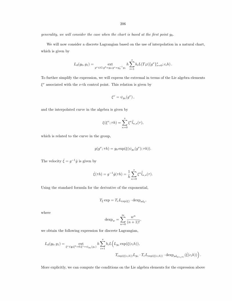
We will now consider a discrete Lagrangian based on the use of interpolation in a natural chart,

which is given by

Ld(g0, g1) = extgν∈G;g0=g0;gs=g−1

0 g1

hs∑i=1

biL(Tϕ(gνsν=0; cih) .

To further simplify the expression, we will express the extremal in terms of the Lie algebra elements

ξν associated with the ν-th control point. This relation is given by

ξν = ψg0(gν) ,

and the interpolated curve in the algebra is given by

ξ(ξν ; τh) =s∑

κ=0

ξκ lκ,s(τ),

which is related to the curve in the group,

g(gν ; τh) = g0 exp(ξ(ψg0(gν); τh)).

The velocity ξ = g−1g is given by

ξ(τh) = g−1g(τh) =1h

s∑κ=0

ξκ˙lκ,s(τ).

Using the standard formula for the derivative of the exponential,

Tξ exp = TeLexp(ξ) · dexpadξ,

where

dexpw =∞∑n=0

wn

(n+ 1)!,

we obtain the following expression for discrete Lagrangian,

Ld(g0, g1) = extξν∈g;ξ0=0;ξs=ψg0 (g1)

hs∑i=1

biL(Lg0 exp(ξ(cih)),

Texp(ξ(cih))Lg0 · TeLexp(ξ(cih)) · dexpadξ(cih)(ξ(cih))

).

More explicitly, we can compute the conditions on the Lie algebra elements for the expression above

207

to be extremal. This implies that

Ld(g0, g1) = hs∑i=1

biL(Lg0 exp(ξ(cih)), Texp(ξ(cih))Lg0 · TeLexp(ξ(cih)) · dexpadξ(cih)

(ξ(cih)))

with ξ0 = 0, ξs = ψg0(g1), and the other Lie algebra elements implicitly defined by

0 = hs∑i=1

bi

[∂L

∂g(cih)Texp(ξ(cih))Lg0 · TeLexp(ξ(cih)) · dexpadξ(cih)

lν,s(ci)

+1h

∂L

∂g(cih)T 2

exp(ξ(cih))Lexp(ξ(cih)) · T

2e Lexp(ξ(cih)) · ddexpadξ(cih)

˙lν,s(ci)

],

for ν = 1, . . . , s− 1, and where

ddexpw =∞∑n=0

wn

(n+ 2)!.

This expression for the higher-order discrete Lagrangian, together with the discrete Euler–Lagrange

equation,

D2Ld(g0, g1) +D1Ld(g1, g2) = 0 ,

yields a higher-order Lie group variational integrator.

5.4 Higher-Order Discrete Euler–Poincare Equations

In this section, we will apply discrete Euler–Poincare reduction (see, for example, Marsden et al.

[1999]) to the Lie group variational integrator we derived previously, to construct a higher-order

generalization of discrete Euler–Poincare reduction.

5.4.1 Reduced Discrete Lagrangian

We first proceed by computing an expression for the reduced discrete Lagrangian in the case when

the Lagrangian is G-invariant. Recall that our discrete Lagrangian uses G-equivariant interpolation,

which, when combined with the G-invariance of the Lagrangian, implies that the discrete Lagrangian

is G-invariant as well. We compute the reduced discrete Lagrangian,

ld(g−10 g1) ≡ Ld(g0, g1)

= Ld(e, g−10 g1)

= extξν∈g;ξ0=0;ξs=log(g−1

0 g1)h

s∑i=1

biL(Le exp(ξ(cih)),

Texp(ξ(cih))Le · TeLexp(ξ(cih)) · dexpadξ(cih)(ξ(cih))

)

208

= extξν∈g;ξ0=0;ξs=log(g−1

0 g1)h

s∑i=1

biL(

exp(ξ(cih)), TeLexp(ξ(cih)) · dexpadξ(cih)(ξ(cih))

).

Setting ξ0 = 0, and ξs = log(g−10 g1), we can solve the stationarity conditions for the other Lie

algebra elements ξνs−1ν=1 using the following implicit system of equations,

0 = hs∑i=1

bi

[∂L

∂g(cih)TeLexp(ξ(cih)) · dexpadξ(cih)

lν,s(ci)

+1h

∂L

∂g(cih)T 2

e Lexp(ξ(cih)) · ddexpadξ(cih)

˙lν,s(ci)

]

where ν = 1, . . . , s− 1.

This expression for the reduced discrete Lagrangian is not fully satisfactory however, since it

involves the Lagrangian, as opposed to the reduced Lagrangian. If we revisit the expression for the

reduced discrete Lagrangian,

ld(g−10 g1) = ext

ξν∈g;ξ0=0;ξs=log(g−10 g1)

h

s∑i=1

biL(

exp(ξ(cih)), TeLexp(ξ(cih)) · dexpadξ(cih)(ξ(cih))

),

we find that by G-invariance of the Lagrangian, each of the terms in the summation,

L(

exp(ξ(cih)), TeLexp(ξ(cih)) · dexpadξ(cih)(ξ(cih))

),

can be replaced by

l(

dexpadξ(cih)(ξ(cih))

),

where l : g → R is the reduced Lagrangian given by

l(η) = L(Lg−1g, TLg−1 g) = L(e, η),

where η = TLg−1 g ∈ g.

From this observation, we have an expression for the reduced discrete Lagrangian in terms of the

reduced Lagrangian,

ld(g−10 g1) = ext

ξν∈g;ξ0=0;ξs=log(g−10 g1)

hs∑i=1

bil(

dexpadξ(cih)(ξ(cih))

).

As before, we set ξ0 = 0, and ξs = log(g−10 g1), and solve the stationarity conditions for the other

209

Lie algebra elements ξνs−1ν=1 using the following implicit system of equations,

0 = hs∑i=1

bi

[∂l

∂η(cih) ddexpadξ(cih)

˙lν,s(ci)

],

where ν = 1, . . . , s− 1.

5.4.2 Discrete Euler–Poincare Equations

As shown above, we have constructed a higher-order reduced discrete Lagrangian that depends on

fkk+1 ≡ gkg−1k+1.

We will now recall the derivation of the discrete Euler–Poincare equations, introduced in Marsden

et al. [1999]. The variations in fkk+1 induced by variations in gk, gk+1 are computed as follows,

δfkk+1 = −g−1k δgkgk−1gk+1 + g−1

k δgk+1

= TRfkk+1(−g−1k δgk + Adfkk+1 gk+1δgk+1) .

Then, the variation in the discrete action sum is given by

δS =N−1∑k=0

l′d(fkk+1)δfkk+1

=N−1∑k=0

l′d(fkk+1)TRfkk+1(−g−1k δgk + Adfkk+1 gk+1δgk+1)

=N−1∑k=1

[l′d(fk−1k)TRfk−1k

Adfk−1k−l′d(fkk+1)TRfkk+1

]ϑk ,

with variations of the form ϑk = g−1k δgk. In computing the variation of the discrete action sum, we

have collected terms involving the same variations, and used the fact that ϑ0 = ϑN = 0. This yields

the discrete Euler–Poincare equation,

l′d(fk−1k)TRfk−1kAdfk−1k

−l′d(fkk+1)TRfkk+1 = 0, k = 1, . . . , N − 1.

For ease of reference, we will recall the expressions from the previous subsection that define the

higher-order reduced discrete Lagrangian,

ld(fkk+1) = hs∑i=1

bil(

dexpadξ(cih)(ξ(cih))

),

210

where

ξ(ξν ; τh) =s∑

κ=0

ξκ lκ,s(τ) ,

and

ξ0 = 0 ,

ξs = log(fkk+1) ,

and the remaining Lie algebra elements ξνs−1ν=1, are defined implicitly by

0 = hs∑i=1

bi

[∂l

∂η(cih) ddexpadξ(cih)

˙lν,s(ci)

],

for ν = 1, . . . , s− 1, and where

ddexpw =∞∑n=0

wn

(n+ 2)!.

When the discrete Euler–Poincare equation is used in conjunction with the higher-order reduced

discrete Lagrangian, we obtain the higher-order Euler–Poincare equations.

5.5 Higher-Order Symplectic-Energy-Momentum Variational

Integrators

In this section, we will generalize our new derivation of the symplectic-energy-momentum preserving

variational integrators (see, Kane et al. [1999]) to yield integrators with higher-order accuracy.

As before, we consider a piecewise interpolation, with both the control points in the field variables,

qνi , and the endpoints of the interval, h0i , h

1i , as degrees of freedom. The continuity conditions for

this function space are qsi = q0i+1, and h1i = h0

i+1. Then, we have that the discrete action is given by

Sd =N−1∑i=0

(h1i − h0

i )s∑j=1

bjL(qi(cj(h1i − h0

i ); qνi ), qi(cj(h

1i − h0

i ); qνi ))

−N−2∑i=0

λi(qsi − q0i+1)−N−2∑i=0

ωi(h1i − h0

i+1),

where

qi(τ(h1i − h0

i ); qνi ) =

s∑κ=0

qκi lκ,s(τ),

211

qi(τ(h1i − h0

i ); qνi ) =

1h1i − h0

i

s∑κ=0

qκi˙lκ,s(τ).

To simplify the expressions, we define hi ≡ h1i − h0

i . Then, the variational equations are given by

0 =s∑j=1

bjL(qi(cjhi), qi(cjhi))− hi

s∑j=1

bj∂L

∂q(cjhi)

1hiqi(cjhi)− ωi, for i = 0, . . . , N − 2,

0 =−s∑j=1

bjL(qi(cjhi), qi(cjhi)) + hi

s∑j=1

bj∂L

∂q(cjhi)

1hiqi(cjhi) + ωi−1, for i = 1, . . . , N − 1,

0 =his∑j=1

bj

[∂L

∂q(cjhi)ls,s(cj) +

1hi

∂L

∂q(cjhi)

˙ls,s(cj)

]− λi, for i = 0, . . . , N − 2,

0 =his∑j=1

bj

[∂L

∂q(cjhi)l0,s(cj) +

1hi

∂L

∂q(cjhi)

˙l0,s(cj)

]+ λi−1, for i = 1, . . . , N − 1,

0 =his∑j=1

bj

[∂L

∂q(cjhi)lν,s(cj) +

1hi

∂L

∂q(cjhi)

˙lν,s(cj)

],

for i = 0, . . . , N − 1,ν = 1, . . . , s− 1,

qsi =q0i+1, for i = 0, . . . , N − 2,

h1i =h0

i+1, for i = 0, . . . , N − 2.

We can eliminate the Lagrange multipliers, to yield

0 =s∑j=1

bjL(qi(cjhi), qi(cjhi))−s∑j=1

bj∂L

∂q(cjhi)qi(cjhi)

+s∑j=1

bjL(qi−1(cjhi−1), qi−1(cjhi−1))

−s∑j=1

bj∂L

∂q(cjhi−1)qi−1(cjhi−1), for i = 1, . . . , N − 1,

0 =his∑j=1

bj

[∂L

∂q(cjhi)ls,s(cj) +

1hi

∂L

∂q(cjhi)

˙ls,s(cj)

]

+ hi−1

s∑j=1

bj

[∂L

∂q(cjhi−1)l0,s(cj) +

1hi−1

∂L

∂q(cjhi−1)

˙l0,s(cj)

], for i = 1, . . . , N − 1,

0 =his∑j=1

bj

[∂L

∂q(cjhi)lν,s(cj) +

1hi

∂L

∂q(cjhi)

˙lν,s(cj)

],

for i = 0, . . . , N − 1,ν = 1, . . . , s− 1,

qsi =q0i+1, for i = 0, . . . , N − 2,

h1i =h0

i+1, for i = 0, . . . , N − 2.

212

If we define the discrete Lagrangian as follows,

Ld(qi, qi+1, hi) ≡ hi

s∑j=1

bjL(qi(cjhi), qi(cjhi)),

where

qi(τhi; qνi ) =s∑

κ=0

qκi lκ,s(τ),

qi(τhi; qνi ) =1hi

s∑κ=0

qκi˙lκ,s(τ),

and q0i = qi, qsi = q1, and the remaining terms were defined implicitly by

0 = hi

s∑j=1

bj

[∂L

∂q(cjhi)lν,s(cj) +

1hi

∂L

∂q(cjhi)

˙lν,s(cj)

],

then the equations reduce to the following,

Ed(qi, qi+1, hi) = − ∂

∂hi[Ld(qi, qi+1, hi)],

Ed(qi, qi+1, hi) = Ed(qi+1, qi+2, hi+1),

0 = D2Ld(qi, qi+1, hi) +D1Ld(qi+1, qi+2, hi+1).

which is a higher-order symplectic-energy-momentum variational integrator.

Solvability of the Energy Equation. It should be noted that the discrete energy conservation

equation is not necessarily solvable, in general, particularly near stationary points. This issue is

discussed in Kane et al. [1999]; Lew et al. [2004], and can be addressed by reformulating the discrete

energy conservation equation as an optimization problem that chooses the time step by minimizing

the discrete energy error squared. Clearly, reformulating the discrete energy conservation equation

yields the desired behavior whenever the discrete energy conservation equation can be solved, while

allowing the computation to proceed when discrete energy conservation cannot be achieved, albeit

with a slight energy error in that case. This does not degrade performance significantly, since

instances in which discrete energy conservation cannot be achieved are rare.

5.6 Spatio-Temporally Adaptive Variational Integrators

As is the case with all inner approximation techniques in numerical analysis, the quality of the

numerical solution we obtain is dependent on the rate at which the sequence of finite-dimensional

213

function spaces approximates the actual solution as the number of degrees of freedom is increased.

For problems that exhibit shocks, nonlinear approximation spaces (see, for example, DeVore

[1998]), as opposed to linear approximation spaces, are clearly preferable. Adaptive techniques

have been developed in the context of finite elements under the name of r-adaptivity and moving

finite elements (see, for example, Baines [1995]), and has been developed in a variational context

for elasticity in Thoutireddy and Ortiz [2003]. The standard motivation in discrete mechanics to

introduce function spaces that have degrees of freedom associated with the base space is to achieve

energy or momentum conservation, as discussed in §5.5, or Kane et al. [1999]; Oliver et al. [2004].

However, if the solution to be approximated exhibits shocks, nonlinear approximation techniques

achieve better results for a given number of degrees of freedom.

In this section, we will sketch the use of regularizing transformations of the base space, to achieve

a computational representation of sections of the configuration bundle that will yield more accurate

numerical results.

Consider the situation when we are representing a characteristic function using piecewise spline

interpolation. We show in Figure 5.2, the difference between linear and nonlinear approximation of

the characteristic function.

(a) Using equispaced nodes (b) Using adaptive nodes

Figure 5.2: Linear and nonlinear approximation of a characteristic function.

When the derivatives of the solution vary substantially in a spatially distributed manner, we

obtain additional accuracy, for a fixed representation cost, if we allow nodal points to cluster near

regions of high curvature. It is therefore desirable to consider variational integrators based on

function spaces that are parameterized by both the position of the nodal points on the base space,

as well as the field values over the nodes.

This is represented by having a regular grid for the computational domain R, which is then

mapped to the physical base space X , as shown in Figure 5.3.

214

7→

Figure 5.3: Mapping of the base space from the computational to the physical domain.

The sections of the configuration bundle factor as follows,

Y

R ϕ//

q>>~~~~~~~X

q

OO

The mapping ϕ : R → X results in a regularized computational representation q : R → Y of the

original section q : X → Y . The relationship between the discrete section of the configuration bundle

and its computational representation is illustrated in Figure 5.4.

ϕ//

q

OO

q

OO

Figure 5.4: Factoring the discrete section.

The action integral is then given by

S(q) =∫XL(j1q) =

∫RL(j1q)|Dϕ|.

Thus, even though q : X → Y may exhibit shocks, the computational representation we work with,

q : R → Y , is substantially more regular, and consequently, a numerical quadrature scheme in R

215

applied to ∫RL(j1q)|Dϕ|

is significantly more accurate than the corresponding numerical quadrature scheme in X applied to

∫XL(j1q).

As such, spatio-temporally adaptive variational integrators achieve increased accuracy by allowing

the accurate representation of shock solutions using an adapted free knot representation, while using

a smooth computational representation to compute the action integral.

5.7 Multiscale Variational Integrators

In the work on multiscale finite elements (MsFEM), introduced and developed in Hou and Wu [1999];

Efendiev et al. [2000]; Chen and Hou [2003], shape functions that are solutions of the fast dynamics

in the absence of slow forces are constructed to yield finite element schemes that achieve convergence

rates that are independent of the ratio of fast to slow scales.

In constructing a multiscale variational integrator, we need to choose finite-dimensional function

spaces that do a good job of approximating the fast dynamics of the problem, when the slow variables

are frozen. In addition, we require an appropriate choice of numerical quadrature scheme to be able

to evaluate the action, which involves integrating a highly-oscillatory Lagrangian. In this section,

we will discuss how to go about making such choices of function spaces and quadrature methods.

We will start with a discussion of the multiscale finite element method, to illustrate the impor-

tance of a good choice of shape functions in computing solutions to problems with multiple scales.

After that, we will walk through the construction of a multiscale variational integrator for the case

of a planar pendulum with a stiff spring. Finally, we will discuss how we might proceed if we do not

possess knowledge of which variables, or forces, are fast or slow.

5.7.1 Multiscale Shape Functions

We will illustrate the idea of constructing shape functions that are solutions of the fast dynamics by

introducing a model multiscale second-order elliptic partial differential equation given by

∇ · a(x/ε)∇uε(x) = f(x),

216

with homogeneous boundary conditions. In the one-dimensional case, we can solve for the solution

analytically, and it has the form

uε(x) =∫ x

0

F (y)a(y/ε)

dy −

∫ 1

0F (y)a(y/ε)dy∫ 1

0dy

a(y/ε)

∫ x

0

dy

a(y/ε),

where F (x) =∫ x0f(y)dy. If we have nodal points at xiNi=0, then the appropriate multiscale shape

functions to adopt in this example is to use shape functions that are solutions of the homogeneous

problem at the element level. These shape functions ϕεi satisfy

∂∂x

(a(x/ε) ∂∂xϕ

εi

)= 0, for xi−1 < x < xi+1;

ϕεi(xi−1) = 0; ϕεi(xi+1) = 0; ϕεi(xi) = 1.

And they have the explicit form given by

ϕεi(x) =

[∫ xi

xi−1

dsa(s/ε)

]−1 [∫ xxi−1

dsa(s/ε)

], x ∈ [xi−1, xi] ;[∫ xi+1

xi

dsa(s/ε)

]−1 [∫ xi+1

xds

a(s/ε)

], x ∈ (xi, xi+1] ;

0, otherwise .

It can be shown that this will yield a numerical scheme that solves exactly for the solution at the

nodal points. This analysis is carried out in Appendix C.

As an example, we will compute the analytical solution for a(x) = 101+0.95 sin(2πx) , f(x) = x2, and

ε = 0.025. This is illustrated in Figure 5.5(a). What is particularly interesting is to compare the

zoomed plot of the exact solution and the multiscale shape function over the same interval, shown

in Figures 5.5(b) and 5.5(c), respectively. The multiscale finite element method is able to achieve

excellent results because the multiscale shape functions are able to capture the fast dynamics well.

In the next subsection, we will discuss how this insight is relevant in the construction of multiscale

variational integrators.

5.7.2 Multiscale Variational Integrator for the Planar Pendulum with a

Stiff Spring

As was shown previously, a shape function that captures the fast dynamics of a multiscale problem

is able to achieve superior accuracy when used for computation. While this idea has primarily been

used for problems with multiple spatial scales, it is natural to consider its application to a problem

with multiple temporal scales, such as the problem of the planar pendulum with a stiff spring, as

illustrated in Figure 5.6.

217

0 0.2 0.4 0.6 0.8 1−0.04

−0.03

−0.02

−0.01

0

0.01

(a) Exact solution

0 0.05 0.1 0.15 0.2 0.25−0.025

−0.02

−0.015

−0.01

−0.005

0

(b) Exact solution (zoomed)

0 0.05 0.1 0.15 0.2 0.250

0.2

0.4

0.6

0.8

1

(c) Multiscale shape function

Figure 5.5: Comparison of the multiscale shape function and the exact solution for the elliptic

problem.

218

Figure 5.6: Planar pendulum with a stiff spring

We will use this example to illustrate the issues that arise in constructing a multiscale variational

integrator. The variables are q = (a, θ), where a is the spring extension, and θ is the angle from the

vertical. The Lagrangian is given by

L(a, θ, a, θ) =m

2(x2 + y2)−mgy − k

2a2,

where

x = (l + a) sin θ,

y = −(l + a) cos θ,

x = a sin θ + θ(l + a) cos θ,

y = −a cos θ + θ(l + a) sin θ.

The Hamilton’s equations for the planar pendulum with a stiff spring are

a =pam,

θ =pθ

m(l + a)2,

pa = −ka+ gm cos θ +m(l + a)θ2,

pθ = −gm(l + a) sin θ.

The timescale arising from the mass-spring system is 2π√m/k. The timescale arising from the

planar pendulum system is 2π√l/g. The ratio of timescales is given by ε =

√mg/kl.

219

Multiscale Shape Function. In this problem, the fast scale is associated with the stiff spring,

and if we set the slow variable θ = 0, we obtain the equation

a =pam

= − k

ma,

which has solutions of the form

a(t) = a0 sin(√

k/m t)

+ a1 cos(√

k/m t).

We will now consider a well-resolved simulation of this system using the ode15s stiff solver from

Matlab, with parameters m = 1, g = 9.81, k = 10000, l = 1, giving a scale separation of ε = 0.0313.

The simulation results are show in Figure 5.7.

0 5 10 15 20−1

−0.5

0

0.5

1

(a) a(t)

0 5 10 15 20−2

−1

0

1

2

(b) θ(t)

0 0.2 0.4 0.6 0.8 1−1

−0.5

0

0.5

1

(c) a(t) (zoomed)

0 0.2 0.4 0.6 0.8 1−1

−0.5

0

0.5

1

(d) 0.5 cos“p

k/m t”

Figure 5.7: Comparison of the multiscale shape function and the exact solution for the planar

pendulum with a stiff spring.

Clearly, if we wish to choose time steps that do not resolve the fast oscillations in a, but do

resolve the slow oscillations in θ, it would be desirable to include sin(√

k/m t), and cos

(√k/m t

)in the finite-dimensional function space used to interpolate a(t).

220

Evaluating the Discrete Lagrangian. Since we have chosen time steps that do not resolve the

fast oscillations, it follows that over the interval [0, h], the Lagrangian will oscillate rapidly as well.

In computing the discrete Lagrangian, it is therefore necessary to ensure that this highly-oscillatory

integral is well-approximated.

It is conventional wisdom, in numerical analysis, that the numerical quadrature of highly-

oscillatory integrals is a challenging problem requiring the use of many function evaluations. Re-

cently, there has been a series of papers, Iserles [2003a,b, 2004]; Iserles and Nørsett [2004], that pro-

vides an analysis of Filon-type quadrature schemes that provide an efficient and accurate method

of evaluating such integrals. The method is applicable to weighted integrals as well, but we will

summarize the results from §3 of Iserles [2003a] restricted to unweighted integrals, and refer the

reader to the original reference for an in-depth discussion and analysis.

The Filon-type method aims to evaluate an integral of the form

Ih[f ] =∫ h

0

f(x)eiωxdx = h

∫ h

0

f(hx)eiωxdx.

Given a set of distinct quadrature points, c1 < c2 < · · · < cν in [0, 1], the Filon-type quadrature

method is given by

QFh [f ] = hν∑i=1

bi(ihω)f(cih),

where

bi(ihω) =∫ 1

0

li(x)eihωxdx,

and li are the Legendre polynomials. Here, we draw attention to the fact that the quadrature weights

are dependent on hω.

If the quadrature points correspond to Gauss-Christoffel quadrature of order p, then the error

for the Filon-type method is given as follows.

O(hp+1), if hω 1

O(hν), if hω = O(1)

O(hν+1/(hω)), if hω 1

O(hν+1/(hω)2), if hω 1, c1 = 0, cν = 1.

Clearly, for highly-oscillatory functions, the last case, which corresponds to the Lobatto quadrature

points, is most desirable. Thus, it is appropriate to use the Filon-Lobatto method to evaluate the

discrete Lagrangian in our case.

221

Discrete Variational Equations. As we discussed previously, instead of looking for stationary

solutions to the discrete Hamilton’s principle in polynomial spaces, we will consider solutions that

are piecewise of the form

q(t; pj, ω, a0, a1) =(∑n

j=0pjt

j)

(1 + a0 sin(ωt) + a1 cos(ωt)) .

This function space approximates the highly-oscillatory nature of the solution well, in contrast

to a polynomial function space, thereby avoiding approximation-theoretic errors. The degrees of

freedom in this function space are pj, ω, a0, and a1. Since there are no distinguished degrees of

freedom that are responsible for the endpoint values of the curve, we need to impose continuity at

the nodes using a Lagrange multiplier. The augmented discrete action is given by

Sd =N−1∑i=0

∫ h

0

L(j1qi(t; pij, ωi, ai0, ai1))dt

+N−2∑i=0

λi(qi(h; pij, ωi, ai0, ai1)− qi+1(0; pi+1j , ωi+1, ai+1

0 , ai+11 )) ,

where each of the integrals are evaluated using the Filon-Lobatto method. Taking variations with

respect to the degrees of freedom yields an update map,

(pij, ωi, ai0, ai1

)7→(pi+1j , ωi+1, ai+1

0 , ai+11

),

which gives the multiscale variational integrator for the planar pendulum with a stiff spring.

5.7.3 Computational Aspects

Multiscale variational integrators have the advantage of directly accounting for the contribution of

the fast dynamics, thereby allowing the scheme to use significantly larger time-steps, while maintain-

ing accuracy and stability. It is possible to take advantage of knowledge about which of the variables,

or forces, are fast or slow, by using a low degree polynomial and oscillatory functions for the fast

variables, and a higher-order polynomial for the slow variables. In the absence of such information,

it is appropriate to use a function space with both polynomials and oscillatory functions, and apply

it to all the variables.

Recall that the Filon-type method has quadrature coefficients that depend on the frequency. As

such, the initial fast frequency has to be estimated numerically using a fully resolved computation

for a short period of time. Since both the function space and the quadrature weights depend on

the fast frequency ω, the resulting scheme is implicit and fairly nonlinear, and as such, it may be

expensive for large systems.

222

5.8 Pseudospectral Variational Integrators

The use of spectral expansions of the solution in space are particularly appropriate for highly accurate

simulations of the evolution of smooth solutions, such as those arising from quantum mechanics. We

will introduce pseudospectral variational integrators, and consider the Schrodinger equation as an

example.

In particular we will adopt the tensor product of a spectral expansion in space, and a polynomial

expansion in time. For example, we could have an interpolatory function of the form

ψ(x, (τ + l)∆t) =12π

N/2∑′

k=−N/2

eikx((1− τ)vlk + τ vl+1

k

),

which is the tensor product of a discrete Fourier expansion in space, and linear interpolation in time.

Here, the∑′ notation denotes a weighted sum where the terms with indices ±N/2 are weighted by

1/2, and the other terms are weighted by 1. See page 19 of Trefethen [2000] for a discussion of why

this is necessary to fix an issue with derivatives of the interpolant.

The degrees of freedom are given by vlk, which are the discrete Fourier coefficients. We will later

see how such an interpolation can be applied to the Schrodinger equation. The action integral can

be exactly evaluated for this class of shape functions, as we will see below.

It is straightforward to generalize the pseudospectral approach we present in this section to

a spectral variational integrator, with discrete Fourier expansions in space for periodic domains,

or Chebyshev expansions in space for non-periodic domains, and Chebyshev expansions in time.

This will however result in all the degrees of freedom on the space-time mesh being coupled, and

is therefore substantially more expensive computationally than the pseudospectral method. The

payoff for adopting the spectral approach is spectral accuracy, which is accuracy beyond all orders.

5.8.1 Variational Derivation of the Schrodinger Equation

Let H be a complex Hilbert space, for example, the space of complex-valued functions ψ on R3 with

the Hermitian inner product,

〈ψ1, ψ2〉 =∫ψ1(x)ψ2(x)d

3x ,

where the overbar denotes complex conjugation. We will present a Lagrangian derivation of the

Schrodinger equation, following worked example 9.1 on pages 568–569 of Jose and Saletan [1998].

Consider the Lagrangian density L given by

L(j1ψ) =i~2ψψ − ψψ − Hψψ,

223

where H : H → H is given by

Hψ = − ~2

2m∇2ψ + V ψ,

which yields

L(j1ψ) =i~2ψψ − ψψ − ~2

2m∇ψ · ∇ψ − V ψψ.

We take ψ,ψ as independent variables, and compute,

δ

∫Ldt =

∫ [(∂L∂ψ

δψ +∂L∂ψ

δψ +∂L∂∇ψ

δ∇ψ

)+

(∂L∂ψ

δψ +∂L∂ψ

δψ +∂L∂∇ψ

δ∇ψ

)]d3xdt

=∫ [(

∂L∂ψ

− ∂

∂t

∂L∂ψ

−∇ · ∂L∂∇ψ

)δψ +

(∂L∂ψ

− ∂

∂t

∂L∂ψ

−∇ · ∂L∂∇ψ

)δψ

]d3xdt

=∫ [(

i~2ψ − V ψ +

i~2ψ +

~2

2m∇2ψ

)δψ +

(i~2ψ − V ψ +

i~2ψ +

~2

2m∇2ψ

)δψ

]d3xdt,

where we integrated by parts, and neglected boundary terms as the variations vanish at the boundary

of the space-time region. Since the variations are arbitrary, we obtain the nonrelativistic (linear)

Schrodinger equation as a result,

i~ψ =− ~2

2m∇2 + V

ψ .

We note that the Lagrangian density is invariant under the internal phase shift given by

ψ 7→ eiεψ, ψ 7→ e−iεψ.

The space part of the multi-momentum map is given by

jk =∂L

∂(∂kψ)iψ +

∂L∂(∂kψ)

(−iψ) =i~2

2m(ψ∂kψ − ψ∂kψ),

and the time part is given by

j0 =∂L∂ψ

iψ − ∂L∂ψ

(−iψ) = −~2(ψψ − ψψ).

The norm of the wavefunction is automatically preserved by variational integrators, since the

norm is a quadratic invariant.

5.8.2 Pseudospectral Variational Integrator for the Schrodinger Equation

Consider a periodic domain [0, 2π], discretized with a discrete Fourier series expansion in space, and

a linear interpolation in time. Let N be an even integer, then, our computation is done on the

224

following mesh,

0 π 2π

x1 x2 xN/2 xN−1 xN• • • • • • • • • •

This implies that the grid spacing is given by

h =2πN.

The interpolation is given by

ψ(x, (τ + l)∆t) =12π

N/2∑′

k=−N/2

eikx((1− τ)vlk + τ vl+1

k

),

ψ(x, (τ + l)∆t) =1

2π∆t

N/2∑′

k=−N/2

eikx(vl+1k − vlk

),

ψ(x, (τ + l)∆t) =12π

N/2∑′

k=−N/2

e−ikx((1− τ)¯vlk + τ ¯vl+1

k

),

˙ψ(x, (τ + l)∆t) =1

2π∆t

N/2∑′

k=−N/2

e−ikx(¯vl+1k − ¯vlk

),

and the discrete Fourier transformation is given by

vj =12πh

N∑j=1

e−ikxjvj ,

for k = −N/2 + 1, . . . , N/2, and v−N/2 ≡ vN/2. Recall that

L(j1ψ) =i~2ψψ − ψψ − Hψψ,

where H : H → H is given by

Hψ = − ~2

2m∇2ψ + V ψ.

Furthermore, the potential V is expressed using a discrete Fourier expansion,

V (x) =12π

N/2∑′

k=−N/2

eikxVk .

225

In addition, we will need to introduce a normalization condition, so as to eliminate trivial solutions

of the partial differential equation. The normalization condition is

1 = 〈ψl, ψl〉 =∫ 2π

0

12π

N/2∑′

k=−N/2

eikxvlk

12π

N/2∑′

k=−N/2

e−ikx ¯vlk

dx =12π

N/2∑′′

k=−N/2

vlk¯vlk,

which is enforced using a Lagrange multiplier.

Discrete Action for the Schrodinger Equation. The discrete action in the space-time region

[0, 2π]× [l∆t, (l + 1)∆t] is given by

Sd =∫ (l+1)∆t

l∆t

∫ 2π

0

L(j1ψ)dxdt+ λl(1− 〈ψl, ψl〉)

=∫ (l+1)∆t

l∆t

∫ 2π

0

[i~2ψψ − ψ ˙ψ+

~2

2m∇2ψψ − V ψψ

]dxdt+ λl

1− 12π

N/2∑′′

k=−N/2

vlk¯vlk

=∫ 1

0

∫ 2π

0

i~2

12π∆t

N/2∑′

k=−N/2

eikx(vl+1k − vlk

) 12π

N/2∑′

k=−N/2

e−ikx((1− τ)¯vlk + τ ¯vl+1

k

)−

12π

N/2∑′

k=−N/2

eikx((1− τ)vlk + τ vl+1

k

) 12π∆t

N/2∑′

k=−N/2

e−ikx(¯vl+1k − ¯vlk

)∆t dxdτ

+∫ 1

0

∫ 2π

0

~2

2m

12π

N/2∑′

k=−N/2

(−k2)eikx((1− τ)vlk + τ vl+1

k

)·

12π

N/2∑′

k=−N/2

e−ikx((1− τ)¯vlk + τ ¯vl+1

k

)∆t dxdτ

−∫ 1

0

∫ 2π

0

12π

N/2∑′

k=−N/2

eikxVk

12π

N/2∑′

m=−N/2

eimx((1− τ)vlm + τ vl+1

m

)·

12π

N/2∑′

n=−N/2

e−inx((1− τ)¯vln + τ ¯vl+1

n

)∆t dxdt

+ λl

1− 12π

N/2∑′′

k=−N/2

vlk¯vlk

226

=∫ 1

0

i~2

12π

N/2∑′′

k=−N/2

((vl+1k − vlk)((1− τ)¯vlk + τ ¯vl+1

k )− ((1− τ)vlk + τ vl+1k )(¯vl+1

k − ¯vlk)) dτ

−∫ 1

0

~2

2πk2

2π

N/2∑′′

k=−N/2

((1− τ)vlk + τ vl+1k )((1− τ)¯vlk + τ ¯vl+1

k )

∆t dτ

−∫ 1

0

(12π

)2 −1∑′

n=−N/2

N/2+n∑′

m=−N/2

(Vn−m((1− τ)vlm + τ vl+1

m )((1− τ)¯vln + τ ¯vl+1n )

)

+N/2∑′

n=0

N/2∑′

m=n−N/2

(Vn−m((1− τ)vlm + τ vl+1

m )((1− τ)¯vln + τ ¯vl+1n )

)∆t dτ

+ λl

1− 12π

N/2∑′′

k=−N/2

vlk¯vlk

=i~4π

N/2∑′′

k=−N/2

[vl+1k

¯vlk − vlk¯vl+1k

]− ~2k2∆t

24π2

N/2∑′′

k=−N/2

[vlk(2¯vlk + ¯vl+1

k ) + vl+1k (¯vlk + 2¯vl+1

k )]

− ∆t24π2

−1∑′

n=−N/2

N/2+n∑′

m=−N/2

+N/2∑′

n=0

N/2∑′

m=n−N/2

Vn−m

[vlm(2¯vln + ¯vl+1

n ) + vl+1m (¯vln + 2¯vl+1

n )]

+ λl

1− 12π

N/2∑′′

k=−N/2

vlk¯vlk

,

where we used the fact that ∫ 2π

0

eikxdx = 2πδi0 ,

for k ∈ Z, and we define∑′ as a weighted sum where the terms with indices ±N/2 are weighted

by 1/2, and∑′′ as a weighted sum where the terms with indices ±N/2 are weighted by 1/4. We

should note that using the same approach, it would be possible to exactly evaluate the action integral

for the class of tensor product shape functions with a discrete Fourier expansion in space, and a

polynomial expansion in time. In particular, a similar approach is valid in exactly evaluating the

action integral when we use shape functions that are spectral in both space and time.

Discrete Euler–Lagrange Equations. We are now in a position to compute the discrete Euler–

Lagrange equations associated with the Schrodinger equation when using a tensor product of a

discrete Fourier expansion in space, and a linear interpolation in time.

227

The discrete variational equations are given by

0 =i~4π[¯vl−1j − ¯vl+1

j

]− ~2k2∆t

24π2

[¯vl−1j + 4¯vlj + ¯vl+1

j

]− ∆t

24π2

N/2+j∑′

n=−N/2

Vn−j[¯vl−1n + 4¯vln + ¯vl+1

n

]− λl

2π¯vlj , for j = −N/2 + 1, . . . ,−1,

0 =i~4π[vl+1j − vl−1

j

]− ~2k2∆t

24π2

[vl−1j + 4vlj + vl+1

j

]− ∆t

24π2

N/2+j∑′

n=−N/2

Vj−n[vl−1n + 4vln + vl+1

n

]− λl

2πvlj , for j = −N/2 + 1, . . . ,−1,

0 =i~4π[¯vl−1j − ¯vl+1

j

]− ~2k2∆t

24π2

[¯vl−1j + 4¯vlj + ¯vl+1

j

]− ∆t

24π2

N/2∑′

n=j−N/2

Vn−j[¯vl−1n + 4¯vln + ¯vl+1

n

]− λl

2π¯vlj , for j = 0, . . . , N/2− 1,

0 =i~4π[vl+1j − vl−1

j

]− ~2k2∆t

24π2

[vl−1j + 4vlj + vl+1

j

]− ∆t

24π2

N/2∑′

n=j−N/2

Vj−n[vl−1n + 4vln + vl+1

n

]− λl

2πvlj , for j = 0, . . . , N/2− 1,

0 =i~

16π

[¯vl−1N/2 − ¯vl+1

N/2

]− ~2k2∆t

96π2

[¯vl−1N/2 + 4¯vlN/2 + ¯vl+1

N/2

]− ∆t

48π2

N/2∑′

n=0

Vn−N/2[¯vl−1n + 4¯vln + ¯vl+1

n

]− λl

2π¯vlN/2 ,

0 =i~

16π

[vl+1N/2 − vl−1

N/2

]− ~2k2∆t

96π2

[vl−1N/2 + 4vlN/2 + vl+1

N/2

]− ∆t

48π2

N/2∑′

n=0

VN/2−n[vl−1n + 4vln + vl+1

n

]− λl

2πvlN/2 ,

1 =12π

N/2∑′′

k=−N/2

vlk¯vlk ,

0 = vl−N/2 − vlN/2 ,

0 = ¯vl−N/2 − ¯vlN/2 .

This system of (2N + 3)-equations, allow us to solve for vl+1k , ¯vl+1

k N/2k=−N/2 and λl from initial

data, vl−1k , ¯vl−1

k N/2k=−N/2 and vlk, ¯vlkN/2k=−N/2. As such, this system of equations are an exam-

ple of a spectral in space, second-order in time, pseudospectral variational integrator for the

time-dependent Schrodinger equation. The expressions for the variational integrator for the time-

228

independent Schrodinger equation, which has spectral accuracy in space, are given by

~2k2 ¯vj = −N/2+j∑′

n=−N/2

Vn−j ¯vn − λ¯vj , for j = −N/2 + 1, . . . ,−1,

~2k2vj = −N/2+j∑′

n=−N/2

Vj−nvn − λvj , for j = −N/2 + 1, . . . ,−1,

~2k2 ¯vj = −N/2∑′

n=j−N/2

Vn−j ¯vn − λ¯vj , for j = 0, . . . , N/2− 1,

~2k2vj = −N/2∑′

n=j−N/2

Vj−nvn − λvj , for j = 0, . . . , N/2− 1,

~2k2

2¯vN/2 = −

N/2∑′

n=0

Vn−N/2 ¯vn − λ¯vN/2 ,

~2k2

2vN/2 = −

N/2∑′

n=0

VN/2−nvn − λvN/2,

1 =12π

N/2∑′′

k=−N/2

vk ¯vk ,

vl−N/2 = vlN/2 ,

¯vl−N/2 = ¯vlN/2 .

As mentioned previously, it is possible generalize this approach to construct a fully spectral varia-

tional integrator in space-time, using Chebyshev polynomials to interpolate in time the coefficients

of the discrete Fourier expansion used in the spatial interpolation. The computational cost of imple-

menting such a scheme would be significantly higher, since this would require all the spatio-temporal

degrees of freedom to be solved for simultaneously.

5.9 Conclusions and Future Work

We have introduced the notion of a generalized Galerkin variational integrator, which is based on the

idea of appropriately choosing a finite-dimensional approximation of the section of the configuration

bundle, and approximating the action integral by a numerical quadrature scheme.

In contrast to standard variational methods, that are typically formulated in terms of interpo-

latory schemes parameterized by values of field variables at nodal and internal points, generalized

Galerkin methods utilize function spaces that can be generated by arbitrary degrees of freedom.

This allows the introduction of Lie group methods, and their symmetry reduction using discrete

229

Euler–Poincare reduction, as well as multiscale, and pseudospectral methods. Nonlinear approxi-

mation spaces allow the construction of spatio-temporally adaptive methods, which are better able

to resolve shocks and other kinds of localized discontinuities in the solution.

It would be interesting to compare the performance of pseudospectral variational integrators

with traditional pseudospectral schemes to see if any additional benefits arise from constructing

pseudospectral schemes using a variational approach. More interesting still would be the compar-

ison for fully spectral methods, since both variational and non-variational methods would achieve

spectral accuracy, and it would make a particularly compelling case for variational integrators if

their advantages persist even when compared to numerical methods with spectral accuracy.

Most mesh adaptive methods use the principle of equipartitioning the error of the numerical

scheme over the mesh elements to obtain moving mesh equations. These methods rely on a posteriori

error estimators that are related to the norm in which the accuracy of the numerical method is

measured. While adaptive variational integrators exhibit an equipartitioning principle, in the sense

that the discrete conjugate momentum associated with the horizontal variations are preserved from

element to element in each connected component of the domain, it would be interesting to carefully

explore the question of whether this can be understood as arising from error equipartitioning with

respect to a geometrically motivated error estimator.

While we have only discussed the application of multiscale variational integrators to the case

of ordinary differential equations, it would be natural to consider their generalizations to partial

differential equations, whereby the multiscale shape functions are obtained through well-resolved

solutions of the cell problem, as in the case with multiscale finite elements (see, for example, Hou

and Wu [1999]). In general, short-term simulations at the fine scale can be used to construct

appropriate shape functions to obtain generalized Galerkin variational integrators at a coarser level,

through the use of principal orthogonal decomposition and balanced truncation, for example. This

is consistent with the coarse-fine computational approach proposed in Theodoropoulos et al. [2000],

or the framework of heterogeneous multiscale methods as proposed in E and Engquist [2003].

A natural generalization would be to consider wavelet based variational integrators, as well as

schemes based on conforming, hierarchical, adaptive refinement methods (CHARMS) introduced in

Grinspun et al. [2002] and further developed in Krysl et al. [2003].