Variational Inference of Population Structure in Large … · Variational methods, originally used for approximating intractable integrals, have been used for a wide variety of applications

Variational Inference of Population Structure in Large SNP

Datasets

Anil Raj ∗, Matthew Stephens †, Jonathan K. Pritchard ‡

∗Department of Genetics, Stanford University, Stanford, CA, 94305

†Departments of Statistics and Human Genetics, University of Chicago, Chicago, IL,

60637

‡Departments of Genetics and Biology, Howard Hughes Medical Institute, Stanford, CA,

94305

1

.CC-BY-NC-ND 4.0 International licensepeer-reviewed) is the author/funder. It is made available under aThe copyright holder for this preprint (which was not. http://dx.doi.org/10.1101/001073doi: bioRxiv preprint first posted online Dec. 2, 2013;

http://dx.doi.org/10.1101/001073

http://creativecommons.org/licenses/by-nc-nd/4.0/

Running Head: Population Structure Inference

Key Words: variational inference, population structure

Corresponding Author:

Anil Raj, Matthew Stephens, Jonathan K. Pritchard

[email protected], [email protected], [email protected]

2


http://dx.doi.org/10.1101/001073


Abstract

Tools for estimating population structure from genetic data are now used in a wide variety of

applications in population genetics. However, inferring population structure in large modern

data sets imposes severe computational challenges. Here, we develop efficient algorithms

for approximate inference of the model underlying the STRUCTURE program using a vari-

ational Bayesian framework. Variational methods pose the problem of computing relevant

posterior distributions as an optimization problem, allowing us to build on recent advances in

optimization theory to develop fast inference tools. In addition, we propose useful heuristic

scores to identify the number of populations represented in a dataset and a new hierarchical

prior to detect weak population structure in the data. We test the variational algorithms

on simulated data, and illustrate using genotype data from the CEPH-Human Genome Di-

versity Panel. The variational algorithms are almost two orders of magnitude faster than

STRUCTURE and achieve accuracies comparable to those of ADMIXTURE. Furthermore,

our results show that the heuristic scores for choosing model complexity provide a reason-

able range of values for the number of populations represented in the data, with minimal

bias towards detecting structure when it is very weak. Our algorithm, fastSTRUCTURE, is

freely available online at http://pritchardlab.stanford.edu/structure.html.

3


http://dx.doi.org/10.1101/001073


INTRODUCTION

Identifying the degree of admixture in individuals and inferring the population of origin of

specific loci in these individuals is relevant for a variety of problems in population genet-

ics. Examples include correcting for population stratification in genetic association studies

(Pritchard and Donnelly 2001; Price et al. 2006), conservation genetics (Wasser et al. 2007),

and studying the ancestry and migration patterns of natural populations (Rosenberg et al. 2002;

Reich et al. ; Catchen et al. 2013). With decreasing costs in sequencing and genotyping

technologies, there is an increasing need for fast and accurate tools to infer population struc-

ture from very large genetic data sets.

Principal components analysis (PCA)-based methods for analyzing population structure,

like EIGENSTRAT (Price et al. 2006) and SMARTPCA (Patterson et al. 2006), con-

struct low-dimensional projections of the data that maximally retain the variance-covariance

structure among the sample genotypes. The availability of fast and efficient algorithms for

singular value decomposition has enabled PCA-based methods to become the popular choice

for analyzing structure in genetic data sets. However, while these low-dimensional projec-

tions allow for straightforward visualization of the underlying population structure, it is

not straightforward to derive and interpret estimates for global ancestry of sample indi-

viduals from their projection coordinates (Novembre and Stephens 2008). In contrast,

model-based approaches like STRUCTURE (Pritchard et al. 2000) propose an explicit

generative model for the data based on the assumptions of Hardy-Weinberg equilibrium be-

tween alleles and linkage equilibrium between genotyped loci. Global ancestry estimates are

then computed directly from posterior distributions of the model parameters, as done in

STRUCTURE, or maximum likelihood estimates of model parameters, as done in FRAPPE

(Tang et al. 2005) and ADMIXTURE (Alexander et al. 2009).

STRUCTURE (Pritchard et al. 2000; Falush et al. 2003; Hubisz et al. 2009) takes

a Bayesian approach to estimate global ancestry by sampling from the posterior distribution

over global ancestry parameters using a Gibbs sampler that appropriately accounts for the

4


http://dx.doi.org/10.1101/001073


conditional independence relationships between latent variables and model parameters. Si-

multaneously, the algorithm uses these samples to approximate the log marginal likelihood

of the data by a function of the conditional mean and variance of the Bayesian deviance

given by the data; this approximation is then used to estimate model complexity (i.e., the

number of populations represented in the sample). However, even well-designed sampling

schemes need to generate a large number of posterior samples in order to resolve convergence

and mixing issues and yield accurate estimates of ancestry proportions, greatly increasing

the time complexity of inference for large genotype data sets. To provide faster estimation,

FRAPPE and ADMIXTURE both use a maximum likelihood approach. FRAPPE computes

maximum likelihood estimates of the parameters of the same model using an expectation-

maximization algorithm, while ADMIXTURE computes the same estimates using a sequen-

tial quadratic programming algorithm with a quasi-Newton acceleration scheme. Our goal

in this paper is to adapt a popular approximate inference framework to greatly speed up

inference of population structure while achieving accuracies comparable to STRUCTURE

and ADMIXTURE.

Variational Bayesian inference aims to repose the problem of inference as an optimiza-

tion problem rather than a sampling problem. Variational methods, originally used for

approximating intractable integrals, have been used for a wide variety of applications in

complex networks (Hofman and Wiggins 2008), machine learning (Jordan et al. 1998),

(Blei et al. 2003) and Bayesian variable selection (Logsdon et al. 2010; Carbonetto and Stephens 2012

Variational Bayesian techniques approximate the log marginal likelihood of the data by

proposing a family of tractable parametric posterior distributions (variational distribution)

over hidden variables in the model; the goal is then to find the optimal member of this family

that best approximates the marginal likelihood of the data (see Models and Methods for more

details). Thus, a single optimization problem gives us both an approximate estimate of the

intractable marginal likelihood and approximate analytical forms for the posterior distribu-

tions over unknown variables. Some commonly used optimization algorithms for variational

5


http://dx.doi.org/10.1101/001073


inference include the variational expectation maximization algorithm (Beal 2003), collapsed

variational inference (Teh et al. 2007), and stochastic gradient descent (Sato 2001).

In the Models and Methods section, we briefly describe the model underlying STRUC-

TURE and detail the framework for variational Bayesian inference that we use to infer the

underlying ancestry proportions. We then propose a more flexible prior distribution over a

subset of hidden parameters in the model and demonstrate that estimation of these hyper-

parameters using an empirical Bayesian framework improves the accuracy of global ancestry

estimates when the underlying population structure is more difficult to resolve. Finally, we

describe a scheme to accelerate computation of the optimal variational distributions and

describe a set of scores to evaluate the accuracy of the results and to select the number of

populations underlying the data. In the Applications section, we compare the accuracy and

time complexity of variational inference with those of STRUCTURE and ADMIXTURE on

simulated genotype data sets and demonstrate the results of variational inference on a large

dataset genotyped in the Human Genome Diversity Panel.

MODELS AND METHODS

We now briefly describe our generative model for population structure followed by a detailed

description of the variational framework used for model inference.

Variational inference: Suppose we have N diploid individuals genotyped at L biallelic

loci. A population is represented by a set of allele frequencies at the L loci, Pk ∈ [0, 1]L, k ∈

{1, . . . , K}, where K denotes the number of populations. The allele being represented at

each locus can be chosen arbitrarily. Allowing for admixed individuals in the sample, we

assume each individual to be represented by a K-vector of admixture proportions, Qn ∈

[0, 1]K ,∑

k Qnk = 1, n ∈ {1, . . . , N}. Conditioned on Qn, the population assignments of the

two copies of a locus, Zanl, Z

bnl ∈ {1, . . . , K}, are assumed to be drawn from a multinomial

distribution parametrized by Qn. Conditioned on population assignments, the genotype at

6


http://dx.doi.org/10.1101/001073


each locus Gnl is the sum of two independent Bernoulli distributed random variables, each

representing the allelic state of each copy of a locus and parameterized by population-specific

allele frequencies. The generative process for the sampled genotypes can now be formalized

as:

• p(Zinl = k|Qn) = multinomial(Qn), i ∈ {a, b},∀n, l

• p(Gnl = 0|Zanl = k, Zb

nl = k′, Pl·) = (1− Plk)(1− Plk′)


nl = k′, Pl·) = Plk(1− Plk′) + Plk′(1− Plk)


nl = k′, Pl·) = PlkPlk′

Given the set of sampled genotypes, we can either compute the maximum likelihood esti-

mates of the parameters P and Q of the model (Alexander et al. 2009; Tang et al. 2005)

or sample from the posterior distributions over the unobserved random variables Za, Zb, P,

and Q (Pritchard et al. 2000) to compute relevant moments of these variables.

Variational Bayesian (VB) inference formulates the problem of computing posterior dis-

tributions (and their relevant moments) into an optimization problem. The central aim is

to find an element of a tractable family of probability distributions, called variational distri-

butions, that is closest to the true intractable posterior distribution of interest. A natural

choice of distance on probability spaces is the Kullback-Leibler (KL) divergence, defined for

a pair of probability distributions q(x) and p(x) as

Dkl (q(x)‖p(x)) =

∫

q(x) logq(x)

p(x)dx (1)

Given the asymmetry of the KL divergence, VB inference chooses p(x) to be the intractable

posterior and q(x) to be the variational distribution; this choice allows us to compute ex-

pectations with respect to the tractable variational distribution, often exactly. Except for

unrealistically small problem sizes, the KL divergence with respect to the true posterior

cannot be computed. However, the KL divergence quantifies the tightness of a lower bound

7


http://dx.doi.org/10.1101/001073


to the log marginal likelihood of the data (Beal 2003); i.e., the KL divergence is equal to

the lower bound up to a constant that is a function of only the data and prior parameters.

For any variational distribution q(Za, Zb, P,Q), we have

log p(G|K) = E [q(Za, Zb, Q, P )] +Dkl

(

q(Za, Zb, Q, P )‖p(Za, Zb, Q, P |G))

(2)

where E is a lower bound to the log marginal likelihood of the data, log p(G|K). An approx-

imation to the true intractable posterior distribution can be computed by minimizing the

KL divergence between the true posterior and variational distribution.

q∗ = arg minqDkl

(

q(Za, Zb, Q, P )‖p(Za, Zb, Q, P |G))

= arg minq

(log p(G|K)− E [q])

= arg maxqE [q] (3)

The log marginal likelihood lower bound (LLBO) of the observed genotypes can be written

as

E =∑

Za,Zb

∫

q(Za, Zb, Q, P ) logp(G,Za, Zb, Q, P )

q(Za, Zb, Q, P )dQdP

=∑

Za,Zb

∫

q(Za, Zb, P ) log p(G|Za, Zb, P ) dP +∑

Za,Zb

∫

q(Za, Zb, Q) log p(Za, Zb|Q) dQ

+Dkl (q(Q)‖p(Q)) +Dkl (q(P )‖p(P )) , (4)

where p(Q) is the prior on the admixture proportions and p(P ) is the prior on the allele

frequencies.

We will restrict our optimization over a variational family that explicitly assumes inde-

pendence between the latent variables (Za, Zb) and parameters (P,Q), commonly called the

mean field approximation in the statistical physics (Kadanoff 2009) and machine learning

literature (Jordan et al. 1998)). Since this assumption is certainly not true when inferring

population structure, the true posterior will not be a member of the variational family and we

will only be able to find the fully factorizable variational distribution that best approximates

8


http://dx.doi.org/10.1101/001073


the true posterior. Nevertheless, this approximation significantly simplifies the optimization

problem. Furthermore, we observe empirically that this approximation achieves reasonably

accurate estimates of lower order moments (e.g., posterior mean and variance) when the true

posterior is replaced by the variational distributions (e.g., when computing prediction error

on held-out entries of the genotype matrix). The variational family we choose here is

q(Za, Zb, Q, P ) ≈ q(Za, Zb)q(Q,P ) =∏

n,l

q(Zanl)q(Z

bnl) ·

∏

n

q(Qn) ·∏

lk

q(Plk), (5)

where each factor can then be written as

q(Zanl) = multinomial(Za

nl)

q(Zbnl) = multinomial(Zb

nl)

q(Qn) = Dirichlet(Qn)

q(Plk) = beta(P ulk, P

vlk). (6)

Zanl, Z

bnl, Qn, P u

lk, and P vlk are the parameters of the variational distributions (variational

parameters). The choice of the variational family is restricted only by the tractability of

computing expectations with respect to the variational distributions; here, we choose para-

metric distributions that are conjugate to the distributions in the likelihood function. The

LLBO of the data in terms of the variational parameters is specified in Appendix-A.

Priors: The choice of priors p(Qn) and p(Plk) plays an important role in inference, partic-

ularly when the FST between the underlying populations is small and population structure

is difficult to resolve. Typical genotype datasets contain hundreds of thousands of genetic

variants typed in several hundreds of samples. Given the small sample sizes in these data

relative to underlying population structure, the posterior distribution over population allele

frequencies can be difficult to estimate; thus, the prior over Plk plays a more important role

in accurate inference than the prior over admixture proportions. Throughout this study, we

choose a symmetric Dirichlet prior over admixture proportions; p(Qn) = Dirichlet(

1K1K

)

.

9


http://dx.doi.org/10.1101/001073


Depending on the difficulty in resolving structure in a given dataset, we suggest using

one of three priors over allele frequencies. When the number of samples is sufficiently large

to resolve the underlying population structure, we propose the choice of a flat beta prior

over population-specific allele frequencies at each locus; p(Plk) = beta(1, 1) (we refer to this

prior as “simple prior” throughout the rest of the paper). For genetic data where structure

is difficult to resolve, the F -model for population structure (Falush et al. 2003) proposes

a hierarchical prior, based on a demographic model that allows the allele frequencies of

the populations to have a shared underlying pattern at all loci. Assuming a star-shaped

genealogy where each of the populations simultaneously split from an ancestral population,

the allele frequency at a given locus is generated from a beta distribution centered at the

ancestral allele frequency at that locus, with variance parametrized by a population-specific

drift from the ancestral population (we refer to this prior as “F-prior”).

p(Plk) = beta

(

PAl

1− Fk

Fk

, (1− PAl )

1− Fk

Fk

)

(7)

Alternatively, we propose a hierarchical prior that is more flexible than the F-prior and allows

for more tractable inference, particularly when additional priors on the hyperparameters need

to be imposed. At a given locus, the population-specific allele frequency is generated by a

logistic normal distribution, with the normal distribution having a locus-specific mean and

a population-specific variance (we refer to this prior as “logistic prior”).

Plk =1

1 + exp−Rlk

p(Rlk) = N (µl, λk) (8)

Having specified the appropriate prior distributions, the optimal variational parameters can

be computed by iteratively minimizing the KL divergence (or, equivalently, maximizing the

LLBO) with respect to each variational parameter, keeping the other variational parame-

ters fixed. The LLBO is concave in each parameter; thus, convergence properties of this

iterative optimization algorithm, also called the variational Bayesian expectation maximiza-

tion algorithm, are similar to those of the expectation-maximization algorithm for maximum

10


http://dx.doi.org/10.1101/001073


likelihood problems. The update equations for each of the three models are detailed in the

Appendix-A. Furthermore, when population structure is difficult to resolve, we propose

updating the hyperparameters ((F, PA) for the F-prior and (µ, λ) for the logistic prior) by

maximizing the LLBO with respect to these variables; conditional on these hyperparameter

values, improved estimates for the variational parameters are then computed by minimiz-

ing the KL divergence. Although such a hyperparameter update is based on optimizing a

lower bound on the marginal likelihood, it is likely (although not guaranteed) to increase

the marginal likelihood of the data, often leading to better inference. A natural extension

of this hierarchical prior would be to allow for a full locus-independent variance-covariance

matrix (Pickrell and Pritchard 2012). However, we observed in our simulations that

estimating the parameters of this hierarchical prior encouraged the model to strongly overfit

the data, leading to poor prediction accuracy on held-out data. Thus, we did not consider

this extension in our analyses.

Accelerated variational inference: Similar to the EM algorithm, the convergence of

the iterative algorithm for variational inference can be quite slow. Treating the iterative

update equations for the set of variational parameters θ as a deterministic map Φ(θ(t)), a

globally convergent algorithm with improved convergence rates can be derived by adapting

the Cauchy-Barzilai-Borwein method for accelerating the convergence of linear fixed-point

problems (Raydan and Svaiter 2002) to the nonlinear fixed-point problem given by our

deterministic map (Varadhan and Roland 2008). Specifically, given a current estimate

of parameters θ(t), the new estimate can be written as

θ(t+1)(νt) = θ(t) − 2νt∆t + ν2tHt (9)

where ∆t = Φ(θ(t)) − θ(t), Ht = Φ(Φ(θ(t))) − 2Φ(θ(t)) + θ(t) and νt = −‖∆t‖‖Ht‖

. Note that the

new estimate is a continuous function of νt and the standard variational iterative scheme can

be obtained from 9 by setting νt to −1. Thus, for values of νt close to −1, the accelerated

algorithm retains the stability and monotonicity of standard EM algorithms while sacrificing

11


http://dx.doi.org/10.1101/001073


a gain in convergence rate. When νt < −1, we gain significant improvement in convergence

rate, with two potential problems: (a) the LLBO could decrease, i.e., E(θ(t+1)) < E(θ(t)), and

(b) the new estimate θ(t+1) might not satisfy the constraints of the optimization problem. In

our experiments, we observe the first problem to occur rarely and we resolve this by simply

testing for convergence of the magnitude of difference in LLBO at successive iterations. We

resolve the second problem using a simple back-tracking strategy of halving the distance

between νt and −1: νt ← (νt− 1)/2, until the new estimate θ(t+1) satisfies the constraints of

the optimization problem.

Validation scores: For each simulated data set, we evaluate the accuracy of each algorithm

using two metrics: accuracy of the estimated admixture proportions and the prediction error

for a subset of entries in the genotype matrix that are held-out before estimating the param-

eters. For a given choice of model complexity K, an estimate of the admixture proportions

Q∗ is taken to be the maximum likelihood estimate of Q when using ADMIXTURE, the

maximum a posteriori (MAP) estimate of Q when using STRUCTURE, and the mean of the

variational distribution over Q inferred using fastSTRUCTURE. We measure the accuracy

of Q∗ by computing the Jensen-Shannon (JS) divergence between Q∗ and the true admixture

proportions. The Jensen-Shannon divergence between two probability vectors P and Q is a

bounded distance metric defined as

JSD(P‖Q) =1

2Dkl (P‖M) +

1

2Dkl (Q‖M) , (10)

where M = 12(P + Q), and 0 ≤ JSD(P‖Q) ≤ 1. Note that if the lengths of P and Q are

not the same, the smaller vector is extended by appending zero-valued entries. The mean

admixture divergence is then defined as the minimum over all permutations of population

labels of the mean JS divergence between the true and estimated admixture proportions over

all samples, with higher divergence values corresponding to lower accuracy.

We evaluate the prediction accuracy by estimating model parameters (or posterior distri-

butions over them) after holding out a subsetM of the entries in the genotype matrix. For

12


http://dx.doi.org/10.1101/001073


each held-out entry, the expected genotype is estimated by ADMIXTURE from maximum

likelihood parameter estimates as

Gnl = 2∑

k

P ∗lkQ

∗nk, (11)

where P ∗lk is the maximum likelihood estimate of Plk. The expected genotype given the

variational distributions requires integration over the model parameters and is derived in

Appendix-B. Given the expected genotypes for the held-out entries, for a specified model

complexity K, the prediction error is quantified by the deviance residuals under the binomial

model averaged over all entries.

dK(G, G) =∑

n,l∈M

Gnl logGnl

Gnl

+ (2−Gnl) log2−Gnl

2− Gnl

(12)

Model complexity: ADMIXTURE suggests choosing the value of model complexity K

that achieves the smallest value of dK(G, G), i.e., K∗cv = arg minK dK(G, G). We propose two

additional metrics to select model complexity in the context of variational Bayesian inference.

Assuming a uniform prior on K, the optimal model complexity K∗E is chosen to be the one

that maximizes the LLBO, where the LLBO is used as an approximation to the marginal

likelihood of the data. However, since the difference between the log marginal likelihood

of the data and the LLBO is difficult to quantify, the trend of LLBO as a function of K

cannot be guaranteed to match that of the log marginal likelihood. Additionally, we propose

a useful heuristic to choose K based on the tendency of mean-field variational schemes to

populate only those model components that are essential to explain patterns underlying

the observed data. Specifically, given an estimate of Q∗ obtained from variational inference

executed for a choice of K, we compute the ancestry contribution of each model component

as the mean admixture proportion over all samples, i.e., ck = 1N

∑

nQ∗nk. The number of

relevant model components K∅∁ is then the minimum number of populations that have a

cumulative ancestry contribution of at least 99.99%.

K∅∁ = min{|S| : S ∈ P(K)and

∑

k∈S

ck > 0.9999}, (13)

13


http://dx.doi.org/10.1101/001073


where K = {1, . . . , K} and P(K) is the power set of K. As K increases, K∅∁ tends to

approach a limit that can be chosen as the optimal model complexity K∗∅∁ .

APPLICATIONS

In this section, we compare the accuracy and runtime performance of the variational inference

framework with the results of STRUCTURE and ADMIXTURE both on datasets generated

from the F -model and on the Human Genome Diversity Panel (HGDP) (Rosenberg et al. 2002).

We expect the results of ADMIXTURE to match those of FRAPPE (Tang et al. 2005) since

they both compute maximum likelihood estimates of the model parameters. However, AD-

MIXTURE converges faster than FRAPPE allowing us to compare it with fastSTRUCTURE

using thousands of simulations. In general, we observe that fastSTRUCTURE estimates

ancestry proportions with accuracies comparable to, and sometimes better than, those es-

timated by ADMIXTURE even when the underlying population structure is rather weak.

Furthermore, fastSTRUCTURE is about two orders of magnitude faster than STRUCTURE

and has comparable runtimes to that of ADMIXTURE. Finally, fastSTRUCTURE gives us

a reasonable range of values for the model complexity required to explain structure under-

lying the data, without the need for a cross-validation scheme. Below, we highlight the key

advantages and disadvantages of variational inference in each problem setting.

Simulated datasets: To evaluate the performance of the different learning algorithms, we

generated two groups of simulated genotype datasets, with each genotype matrix consist-

ing of 600 samples and 2500 loci. The first group was used to evaluate the accuracy of

the algorithms as a function of strength of the underlying population structure while the

second group was used to evaluate accuracy as a function of number of underlying popula-

tions. Although the size of each genotype matrix was kept fixed in these simulations, the

performance characteristics of the algorithms are expected to be similar if the strength of

population structure is kept fixed and the dataset size is varied (Patterson et al. 2006).

14


http://dx.doi.org/10.1101/001073


For the first group, the samples were drawn from a 3-population demographic model

as shown in Figure 1a. The edge weights correspond to the parameter F in the model

that quantifies the genetic drift of each of the three current populations from an ancestral

population. We introduced a scaling factor r ∈ [0, 1] that quantifies the resolvability of

population structure underlying the samples. Scaling F by r reduces the amount of drift

of current populations from the ancestral population; thus, structure is difficult to resolve

when r is close to 0, while structure is easy to resolve when r is close to 1. For each r ∈

{0.05, 0.10, . . . , 0.95, 1}, we generated 50 replicate datasets. The ancestral allele frequencies

πA for each dataset were drawn from the frequency spectrum computed using the HGDP

panel to simulate allele frequencies in natural populations. For each dataset, the allele

frequency at a given locus for each population was drawn from a beta distribution with

mean πAl and variance rFkπ

Al (1− πA

l ), and the admixture proportions for each sample were

drawn from a symmetric Dirichlet distribution, namely Dirichlet( 110

13), in order to simulate

small amounts of gene flow between the three populations. Finally, 10% of the samples in

each dataset, randomly selected, were assigned to one of the three populations with zero

admixture.

For the second group, the samples were drawn from a star-shaped demographic model

with Kt populations. Each population was assumed to have equal drift from an ancestral

population, with the F parameter fixed at either 0.01 to simulate weak structure or 0.04

to simulate strong structure. The ancestral allele frequencies were simulated similar to

the first group and 50 replicate datasets were generated for this group for each value of

Kt ∈ {1, . . . , 5}. We executed ADMIXTURE and fastSTRUCTURE for each dataset with

various choices of model complexity; for datasets in the first group, model complexity K ∈

{1, . . . , 5}, and for those in the second group K ∈ {1, . . . , 8}. We executed ADMIXTURE

with default parameter settings; with these settings the algorithm terminates when the

increase in log likelihood is less than 10−4 and computes prediction error using 5-fold cross-

validation. fastSTRUCTURE was executed with a convergence criterion of change in the

15


http://dx.doi.org/10.1101/001073


per-genotype log marginal likelihood lower bound |∆E| < 10−8. We held out 20 random

disjoint genotype sets each containing 1% of entries in the genotype matrix and used the

mean and standard error of the deviance residuals for these held-out entries as an estimate

of the prediction error.

For each group of simulated datasets, we illustrate a comparison of the performance of

ADMIXTURE and fastSTRUCTURE with the simple and the logistic prior. When struc-

ture was easy to resolve, both the F-prior and the logistic prior returned similar results;

however, the logistic prior returned more accurate ancestry estimates when structure was

difficult to resolve. Plots including results using the F-prior are shown in the supplementary

figures. Since ADMIXTURE uses held-out deviance residuals to choose model complexity,

we demonstrate the results of the two algorithms, each using deviance residuals to choose

K, using solid lines in Figures 1 and 2. Additionally, in these figures, we also illustrate the

performance of fastSTRUCTURE, when using the two alternative metrics to choose model

complexity, using blue lines.

Choice of K: Identifying the number of populations needed to explain structure in the

data is a problem of great interest associated with the inference of population structure.

While this commonly has been addressed using cross-validation or a model-selection frame-

work, the problem of identifying a single “correct” number of populations is ill-posed and

strongly dependent on how pertinent the underlying model of population structure is to

a specific study sample (Engelhardt and Stephens 2010). For example, given a set of

individuals sampled from a habitat with spatially continuous population structure, apply-

ing ADMIXTURE or STRUCTURE to the sample genotypes would give us insights into

population structure represented in the data. However, the number of populations returned

by an automatic scheme to select K is not likely to be meaningful in this case, and could

be strongly dependent on the ascertainment of individuals in the dataset and the deviation

of sample genotypes from the strict random-mating model. While identifying a reasonable

16


http://dx.doi.org/10.1101/001073


range of values for K for a given dataset is certainly useful, the specific values of K and the

identified populations need to be interpreted within the context of prior knowledge specific

to the dataset being analyzed.

The manual of the ADMIXTURE code proposes choosing model complexity that min-

imizes the prediction error on held-out data estimated using the mean deviance residuals

reported by the algorithm (K∗cv). In Figure 1b, using the first group of simulations, we

compare the value of K∗cv, averaged over 50 replicate datasets, between the two algorithms

as a function of the resolvability of population structure in the data. We observe that while

deviance residuals estimated by ADMIXTURE robustly identify an appropriate model com-

plexity, the value of K identified using deviance residuals computed using the variational

parameters from fastSTRUCTURE appear to over-estimate the value of K underlying the

data. However, on closer inspection, we observe that the difference in prediction errors

between large values of K are statistically insignificant (Figure 3, middle panels). This

suggests the following heuristic: select the lowest model complexity above which prediction

errors don’t vary significantly.

Alternatively, for fastSTRUCTURE with the simple prior, we propose two additional

metrics for choosing model complexity: (1) K∗E : value of K that maximizes the LLBO of

the entire dataset, and (2) K∗∅∁ : the limiting value, as K increases, of the smallest number

of model components that accounts for almost all of the ancestry in the sample. In Figure

1b, we observe that K∗E has the attractive property of robustly identifying strong structure

underlying the data, while K∗∅∁ identifies additional model components needed to explain

weak structure in the data, with a slight upward bias in complexity when the underlying

structure is extremely difficult to resolve. For the second group of simulations, similar to

results observed for the first group, when population structure is easy to resolve, ADMIX-

TURE robustly identifies the correct value of K (shown in Figure 2a). However, for similar

reasons as before, the use of prediction error with fastSTRUCTURE tends to systemati-

cally overestimate the number of populations underlying the data. In contrast, K∗E and K∗

∅∁

17


http://dx.doi.org/10.1101/001073


match exactly to the true K when population structure is strong. When the underlying

population structure is very weak, K∗E is a severe underestimate of the true K while K∗

∅∁

slightly overestimates the value of K. Surprisingly, K∗cv estimated using ADMIXTURE and

K∗∅∁ estimated using fastSTRUCTURE tend to underestimate the number of populations

when the true number of populations Kt is large, as shown in Figure 2b.

For a new dataset, we suggest executing fastSTRUCTURE for multiple values of K and

estimating (K∗E , K

∗∅∁) to obtain a reasonable range of values for the number of populations

that would explain structure in the data, under the given model. To look for subtle structure

in the data, we suggest executing fastSTRUCTURE with the logistic prior with values for

values of K similar to those identified by using the simple prior.

Accuracy of ancestry proportions: We evaluated the accuracy of the algorithms by

comparing the divergence between the true admixture proportions and the estimated ad-

mixture proportions at the optimal model complexity computed using the above metrics

for each dataset. In Figure 1c, we plot the mean divergence between the true and esti-

mated admixture proportions, over multiple replicates, as a function of resolvability. We

observe that the admixture proportions estimated by fastSTRUCTURE at K∗E have high

divergence; however, this is a result of LLBO being too conservative in identifying K. At

K = K∗cv and K = K∗

∅∁ , fastSTRUCTURE estimates admixture proportions with accura-

cies comparable to, and sometimes better than, ADMIXTURE even when the underlying

population structure is rather weak. Furthermore, the held-out prediction deviances com-

puted using posterior estimates from variational algorithms are consistently smaller than

those estimated by ADMIXTURE (see Figure S3) demonstrating the improved accuracy

of variational Bayesian inference schemes over maximum likelihood methods. Similarly, for

the second group of simulated datasets, we observe in Figures 2c and 2d that the accuracy

of variational algorithms tend to be comparable to or better than that of ADMIXTURE,

particularly when structure is difficult to resolve. When structure is easy to resolve, the

18


http://dx.doi.org/10.1101/001073


increased divergence estimates of fastSTRUCTURE with the logistic prior result from the

upward bias in the estimate of K∗cv; this can be improved by using cross-validation more

carefully in choosing model complexity.

Visualizing ancestry estimates: Having demonstrated the performance of fastSTRUC-

TURE on multiple simulated datasets, we now illustrate the performance characteristics

and parameter estimates using two specific datasets (selected from the first group of simu-

lated datasets), one with strong population structure (r = 1) and one with weak structure

(r = 0.5). In addition to these algorithms, we executed STRUCTURE for these two datasets

using the model of independent allele frequencies in order to directly compare with the results

of fastSTRUCTURE. For each dataset, α was kept fixed to 1K

for all populations, similar

to the prior used for fastSTRUCTURE and each run consisted of 50000 burn-in steps and

50000 MCMC steps. In Figure 3, we illustrate the divergence of admixture estimates and

the prediction error on held-out data each as a function of K. For all choices of K greater

than or equal to the true value, the accuracy of the fastSTRUCTURE, measured using both

admixture divergence and prediction error, is generally comparable to or better than that of

ADMIXTURE and STRUCTURE, even when the underlying population structure is rather

weak. In the right panels of Figure 3, we plot the approximate marginal likelihood of the

data, reported by STRUCTURE, and the optimal LLBO, computed by fastSTRUCTURE,

each as a function of K. We note that the looseness of the bound between STRUCTURE and

fastSTRUCTURE can make the LLBO a less reliable measure to choose model complexity

than the approximate marginal likelihood reported by STRUCTURE, particularly when the

size of the dataset is not sufficient to resolve the underlying population structure.

Figure 4 illustrates the admixture proportions estimated by the different algorithms on

both data sets at two values of K, using Distruct plots (Rosenberg 2004). For the larger

choice of model complexity, we observe that fastSTRUCTURE with the simple prior uses

only those model components that are necessary to explain the data, allowing for automatic

19


http://dx.doi.org/10.1101/001073


inference of model complexity (Mackay 2003). To better illustrate this property of unsuper-

vised Bayesian inference methods, the right panels of Figure 4 show the mean contribution of

ancestry from each model component to samples in the dataset. While ADMIXTURE uses

all components of the model to fit the data, STRUCTURE and fastSTRUCTURE assign

negligible posterior mass to model components that are not required to capture structure in

the data. The number of non-empty model components (K∅∁) automatically identifies the

model complexity required to explain the data; the optimal model complexity K∗∅∁ is then

the mode of all values of K∅∁ computed for different choices of K.

When population structure is difficult to resolve, imposing a logistic prior and estimat-

ing its parameters using the data is likely to increase the power to detect weak structure.

However, estimation of the hierarchical prior parameters by maximizing the approximate

marginal likelihood also makes the model susceptible to overfitting by encouraging a small

set of samples to be randomly, and often confidently, assigned to unnecessary components

of the model. To correct for this, when using the logistic prior, we suggest estimating the

variational parameters with multiple random restarts and using the mean of the parameters

corresponding to the top 5 values of LLBO. In order to ensure consistent population labels

when computing the mean, we permuted the labels for each set of variational parameter esti-

mates to find the permutation with the lowest pairwise Jensen-Shannon divergence between

admixture proportions among pairs of restarts. Admixture estimates computed using this

scheme show improved robustness against overfitting, as illustrated in Figure 4. Moreover,

the pairwise Jensen-Shannon divergence between admixture proportions among all restarts

of the variational algorithms can also be used as a measure of the robustness of their results

and as a signature of how strongly they overfit the data.

Runtime performance: A key advantage of variational Bayesian inference algorithms

compared to inference algorithms based on sampling is the dramatic improvement in time

complexity of the algorithm. To evaluate the runtimes of the different learning algorithms,

20


http://dx.doi.org/10.1101/001073


we generated from the F -model datasets with sample sizes N ∈ {200, 600} and numbers

of loci L ∈ {500, 2500}, each having 3 populations with r = 1. The time complexity of

each of the above algorithms is linear in the number of samples, loci, and populations, i.e.

O(NLK); in comparison, the time complexity of principal components analysis is quadratic

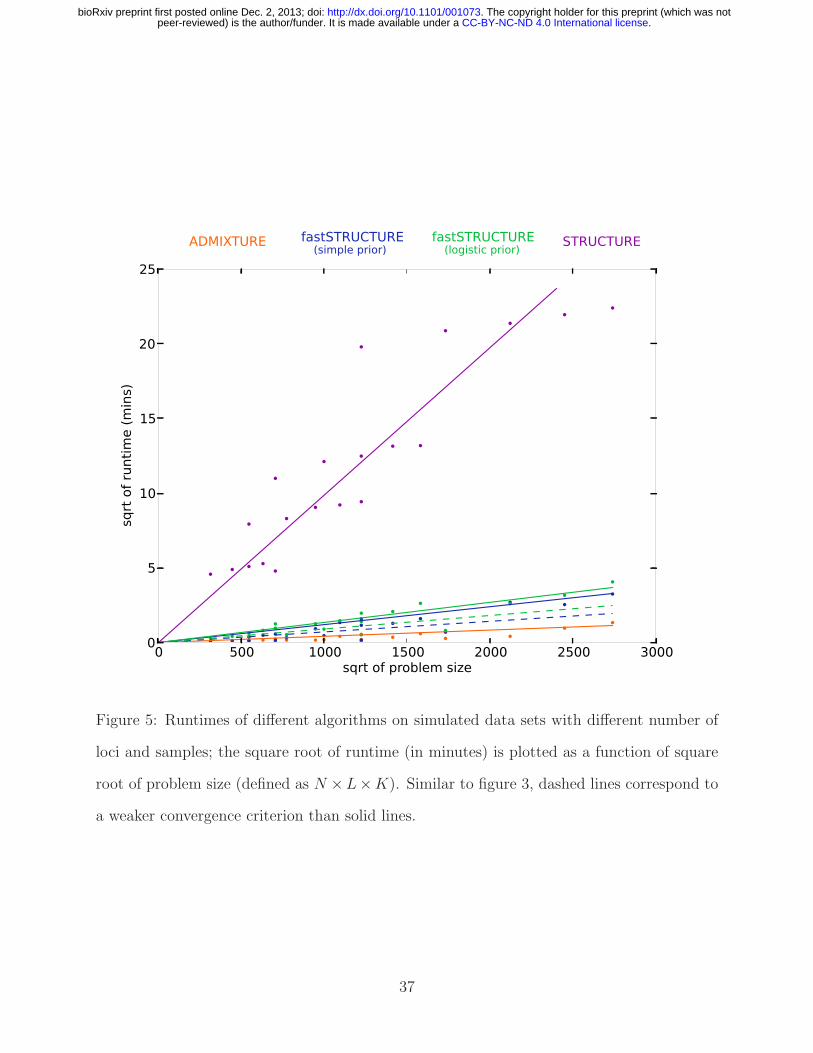
in the number of samples and linear in the number of loci. In Figure 5, the mean runtime

of the different algorithms is shown as a function of problem size defined as N × L × K.

The added complexity of the cost function being optimized in fastSTRUCTURE increases

its runtime when compared to ADMIXTURE. However, fastSTRUCTURE is about two

orders of magnitude faster than STRUCTURE, making it suitable for large datasets with

hundreds of thousands of genetic variants. For example, using a dataset with 1000 samples

genotyped at 500, 000 loci with K = 10, each iteration of our current Python implementation

of fastSTRUCTURE with the simple prior takes about 11 minutes, while each iteration

of ADMIXTURE takes about 16 minutes. Since one would usually like to estimate the

variational parameters for multiple values of K for a new dataset, a faster algorithm that

gives an approximate estimate of ancestry proportions in the sample would be of much

utility, particularly to guide an appropriate choice of K. We observe in our simulations that

a weaker convergence criterion of |∆E| < 10−6 gives us comparably accurate results with

much shorter run times, illustrated by the dashed lines in Figures 3 and 5. Based on these

observations, we suggest executing multiple random restarts of the algorithm with a weak

convergence criterion of |∆E| < 10−5 to rapidly obtain reasonably accurate estimates of

the variational parameters, prediction errors and ancestry contributions from relevant model

components.

HGDP Panel: We now compare the results of ADMIXTURE and fastSTRUCTURE on a

large, well-studied dataset of genotypes at single nucleotide polymorphisms (SNP) genotyped

in the Human Genome Diversity Panel (HGDP) (Li et al. 2008), in which 1048 individuals

from 51 different populations were genotyped using Illumina’s HumanHap650Y platform. We

21


http://dx.doi.org/10.1101/001073


used the set of 938 “unrelated” individuals for the analysis in this paper. For the selected

set of individuals, we removed SNPs that were monomorphic, had missing genotypes in more

than 5% of the samples and failed the Hardy-Weinberg Equilibrium (HWE) test at p < 0.05

cutoff. To test for violations from HWE, we selected three population groups that have rela-

tively little population structure (East Asia, Europe, Bantu Africa), constructed three large

groups of individuals from these populations, and performed a test for HWE for each SNP

within each large group. The final dataset contained 938 samples with genotypes at 657, 143

loci, with 0.1% of the entries in the genotype matrix missing. We executed ADMIXTURE

and fastSTRUCTURE using this dataset with allowed model complexity K ∈ {5, . . . , 15}.

In Figure 6, the ancestry proportions estimated by ADMIXTURE and fastSTRUCTURE at

K = 7 are shown; this value of K was chosen to compare with results reported using the

same dataset with FRAPPE (Li et al. 2008). In contrast to results reported using FRAPPE,

we observe that both ADMIXTURE and fastSTRUCTURE identify the Mozabite, Bedouin,

Palestinian, and Druze populations as very closely related to European populations with

some gene flow from Central-Asian and African populations; this result was robust over

multiple random restarts of each algorithm. Since both ADMIXTURE and FRAPPE max-

imize the same likelihood function, the slight difference in results is likely due to differences

in the modes of the likelihood surface to which the two algorithms converge. A notable

difference between ADMIXTURE and fastSTRUCTURE is in their choice of the 7th popu-

lation – ADMIXTURE splits the Native American populations along a north-south divide

while fastSTRUCTURE splits the African populations into central African and south African

population groups.

Interestingly, both algorithms strongly suggest the existence of additional weak popu-

lation structure underlying the data, as shown in Figure 7. ADMIXTURE, using cross-

validation, identifies the optimal model complexity to be 11; however, the deviance residuals

appear to change very little beyond K = 7 suggesting that the model components identified

at K = 7 explain most of the structure underlying the data. Using LLBO, fastSTRUC-

22


http://dx.doi.org/10.1101/001073


TURE identifies the number of easily resolvable populations to be K∗E = 7, while the K∗

∅∁

estimate suggests the number of populations to be 9. The lowest cross-validation error for

fastSTRUCTURE is achieved at K∗cv = 10; a slight overestimate compared to the model

complexity range suggested by K∗E and K∗

∅∁ .

The admixture proportions estimated at the optimal choices of model complexity using

the different metrics are shown in Figure 8. The admixture proportions estimated at K = 7

and K = 9 are remarkably similar with the Kalash and Karitiana populations being assigned

to their own model components at K = 9. These results demonstrate the ability of LLBO

to identify strong structure underlying the data and that of K∅∁ to identify additional weak

structure that explain variation in the data. At K = 10 (as identified using cross-validation),

we observe that only 9 of the model components are populated. However, the estimated

admixture proportions differ crucially with all African populations grouped together, the

Melanesian and Papuan populations each assigned to their own groups, and the Middle-

Eastern populations represented as predominantly an admixture of Europeans and a Bedouin

sub-population with small amounts of gene flow from Central-Asian populations.

DISCUSSION

Our analyses on simulated and natural datasets demonstrate that fastSTRUCTURE esti-

mates approximate posterior distributions on ancestry proportions two orders of magnitude

faster than STRUCTURE, with ancestry estimates and prediction accuracies that are compa-

rable to those of ADMIXTURE. Posing the problem of inference in terms of an optimization

problem allows us to draw on powerful tools in convex optimization and plays an important

role in the gain in speed achieved by variational inference schemes, when compared to the

Gibbs sampling scheme used in STRUCTURE. In addition, the flexible logistic prior en-

ables us to resolve subtle structure underlying a dataset. The considerable improvement in

runtime with comparable accuracies allows the application of these methods to large geno-

type datasets that are steadily becoming the norm in studies of population history, genetic

23


http://dx.doi.org/10.1101/001073


association with disease, and conservation biology.

The choice of model complexity, or the number of populations required to explain struc-

ture in a dataset, is a difficult problem associated with the inference of population structure.

Unlike in maximum likelihood estimation, the model parameters have been integrated out in

variational inference schemes and optimizing the KL divergence in fastSTRUCTURE does

not run the risk of overfitting. The heuristic scores that we have proposed to identify model

complexity provide a robust and reasonable range for the number of populations underlying

the dataset, without the need for a time-consuming cross-validation scheme.

As in the original version of STRUCTURE, the model underlying fastSTRUCTURE does

not explicitly account for linkage disequilibrium (LD) between genetic markers. While LD

between genotype markers in the genotype dataset will lead us to underestimate the variance

of the approximate posterior distributions, the improved accuracy in predicting held-out

genotypes for the HGDP dataset demonstrates that the underestimate due to un-modeled

LD and the mean field approximation is not too severe. Furthermore, not accounting for

LD appropriately can lead to significant biases in local ancestry estimation, depending on

the sample size and population haplotype frequencies. However, we believe global ancestry

estimates are likely to incur very little bias due to un-modeled LD.

In summary, we have presented a variational framework for fast, accurate inference of

global ancestry of samples genotyped at a large number of genetic markers. For a new dataset,

we recommend executing our program, fastSTRUCTURE, for multiple values of K to obtain

a reasonable range of values for the appropriate model complexity required to explain struc-

ture in the data, as well as ancestry estimates at those model complexities. For improved an-

cestry estimates and to identify subtle structure, we recommend executing fastSTRUCTURE

with the logistic prior at values of K similar to those identified when using the simple prior.

Our program is available for download at http://pritchardlab.stanford.edu/structure.html.

24


http://dx.doi.org/10.1101/001073


APPENDIX-A

Given the parametric forms for the variational distributions and a choice of prior for the

fastSTRUCTURE model, the per-genotype LLBO is given as

E =1

G

∑

n,l

δ(Gnl)

{

∑

k

(E[Zanlk] + E[Zb

nlk]) (I[Gnl = 0]E[log(1− Plk)] + I[Gnl = 2]E[logPlk] + E[logQnk])

+I[Gnl = 1]∑

k

(

E[Zanlk]E[logPlk] + E[Zb

nlk]E[log(1− Plk)])

− E[logZanl]− E[logZb

nl]

}

+∑

l,k

logB(P u

lk, Pvlk)

B(β, γ)+ (β − P u

lk)E[logPlk] + (γ − P vlk)E[log(1− Plk)]

+∑

n

{

∑

k

(αk − Qnk)E[logQnk] + log Γ(αk)− log Γ(Qnk)

}

+ log Γ(Qno)− log Γ(αo)

(A1)

where E[·] is the expectation taken with respect to the appropriate variational distribution,

B(·) is the beta function, Γ(·) is the gamma function, {α, β, γ} are the hyperparameters in

the model, δ(·) is an indicator variable that takes the value of zero if the genotype is missing,

G is the number of observed entries in the genotype matrix, αo =∑

k αk, and Qno =∑

k Qnk.

Maximizing this lower bound for each variational parameter, keeping the other parameters

fixed, gives us the following update equations.

(Za, Zb):

Zanlk ∝ exp

{

ΨaGnl− ψ(P u

lk + P vlk) + ψ(Qnk)− ψ(Qno)

}

(A2)

Zbnlk ∝ exp

{

ΨbGnl− ψ(P u

lk + P vlk) + ψ(Qnk)− ψ(Qno)

}

(A3)

where

ΨaGnl

= I[Gnl = 0]ψ(P vlk) + I[Gnl = 1]ψ(P u

lk) + I[Gnl = 2]ψ(P ulk) (A4)

ΨbGnl

= I[Gnl = 0]ψ(P vlk) + I[Gnl = 1]ψ(P v

lk) + I[Gnl = 2]ψ(P ulk) (A5)

Q:

Qnk = αk +∑

l

δ(Gnl)(Zanlk + Zb

nlk) (A6)

25


http://dx.doi.org/10.1101/001073


(P u, P v):

P ulk = β +

∑

n

(

I[Gnl = 1]Zanlk + I[Gnl = 2](Za

nlk + Zbnlk)

)

(A7)

P vlk = γ +

∑

n

(

I[Gnl = 1]Zbnlk + I[Gnl = 0](Za

nlk + Zbnlk)

)

(A8)

In the above update equations, ψ(·) is the digamma function. When the F-prior is used, the

LLBO and the update equations remain exactly the same, after replacing β with πAl

1−Fk

Fk

and γ with (1− πAl )1−Fk

Fk

. In this case, the LLBO is also maximized with respect to the hy-

perparameter F using the L-BFGS-B algorithm, a quasi-Newton code for bound-constrained

optimization.

When the logistic prior is used, a straightforward maximization of the LLBO no longer

gives us explicit update equations for P ulk and P v

lk. One alternative is to use a constrained

optimization solver, like L-BFGS-B; however, the large number of variational parameters

to be optimized greatly increases the per-iteration computational cost of the inference algo-

rithm. Instead, we propose update equations for P ulk and P v

lk to have a similar form as those

obtained with the simple prior,

P ulk = βlk +

∑

n

I[Gnl = 1]Zanlk + I[Gnl = 2](Za

nlk + Zbnlk) (A9)

P vlk = γlk +

∑

n

I[Gnl = 1]Zbnlk + I[Gnl = 0](Za

nlk + Zbnlk), (A10)

where βlk and γlk implicitly depend on P ulk and P v

lk as follows:

(

ψ′(P ulk)− ψ

′(P ulk + P v

lk))

βlk − ψ′(P u

lk + P vlk)γlk

= −λkψ′(P u

lk)(ψ(P ulk)− ψ(P v

lk)− µl)−1

2λkψ

′′(P ulk)

−ψ′(P ulk + P v

lk)βlk +(

ψ′(P ulk)− ψ

′(P ulk + P v

lk))

γlk

= λkψ′(P v

lk)(ψ(P ulk)− ψ(P v

lk)− µl)−1

2λkψ

′′(P vlk)

(A11)

26


http://dx.doi.org/10.1101/001073


The optimal values for P ulk and P v

lk can be obtained by iterating between the two sets of

equations to convergence. Thus, when the logistic prior is used, the algorithm is implemented

as a nested iterative scheme where for each update of all the variational parameters, there

is an iterative scheme that computes the update for (P u, P v). Finally, the optimal value of

the hyperparameter µ is obtained straightforwardly as

µl =∑

k

λk

(

ψ(P ulk)− ψ(P v

lk))

/

∑

k

λk (A12)

while the optimal λ is computed using a constrained optimization solver.

APPENDIX-B

Given the observed genotypes G, the probability of the unobserved genotype for the nth

sample at the lth locus is given as

p(Ghidnl |G) =

∫

p(Ghidnl |P,Q)p(P,Q|G) dQdP. (A13)

27


http://dx.doi.org/10.1101/001073


Replacing the posterior p(P,Q|G) with the optimal variational posterior distribution, we get

p(Ghidnl = 0) ≈

∫

p(Ghidnl = 0|P,Q)q(P )q(Q) dQdP (A14)

=∑

k,k′

∫

QnkQnk′(1− Plk)(1− Plk′)q(P )q(Q) dQdP (A15)

=∑

k 6=k′

E[QnkQnk′ ](1− E[Plk])(1− E[Plk′ ]) (A16)

+∑

k=k′

E[Q2nk]E[(1− Plk)

2] (A17)

p(Ghidnl = 1) ≈

∫


= 2∑

k,k′

∫

QnkQnk′Plk(1− Plk′)q(P )q(Q) dQdP (A19)

=∑

k 6=k′

E[QnkQnk′ ]E[Plk](1− E[Plk′ ]) (A20)

+∑

k=k′

E[Q2nk]E[Plk(1− Plk)] (A21)

p(Ghidnl = 2) ≈

∫


=∑

k,k′

∫

QnkQnk′PlkPlk′q(P )q(Q) dQdP (A23)

=∑

k 6=k′

E[QnkQnk′ ]E[Plk]E[Plk′ ] (A24)

+∑

k=k′

E[Q2nk]E[P 2

lk], (A25)

28


http://dx.doi.org/10.1101/001073


where

E[QnkQnk′ ] =QnkQnk′

Qno(Qno + 1)(A26)

E[Q2nk] =

Qnk(Qnk + 1)

Qno(Qno + 1)(A27)

E[Plk] =P u

lk

P ulk + P v

lk

(A28)

E[P 2lk] =

P ulk(P

ulk + 1)

(P ulk + P v

lk)(Pulk + P v

lk + 1)(A29)

E[Plk(1− Plk)] =P u

lkPvlk

(P ulk + P v

lk)(Pulk + P v

lk + 1)(A30)

E[(1− Plk)2] =

P vlk(P

vlk + 1)

(P ulk + P v

lk)(Pulk + P v

lk + 1)(A31)

(A32)

The expected genotype can then be straightforwardly computed from these genotype prob-

abilities.

LITERATURE CITED

Alexander, D. H., J. Novembre, and K. Lange, 2009 Fast model-based estimation of

ancestry in unrelated individuals. Genome Research 19 (9): 1655–1664.

Beal, M. J., 2003 Variational Algorithms for Approximate Bayesian Inference. Ph. D.

thesis, Gatsby Computational Neuroscience Unit, University College London.

Blei, D. M., A. Y. Ng, and M. I. Jordan, 2003 Latent dirichlet allocation. Journal of

Machine Learning Research 3: 993–1022.

Carbonetto, P. and M. Stephens, 2012 Scalable variational inference for Bayesian

variable selection in regression, and its accuracy in genetic association studies. Bayesian

Analysis 7 (1): 73–108.

Catchen, J., S. Bassham, T. Wilson, M. Currey, C. O’Brien, Q. Yeates, and

W. A. Cresko, 2013 The population structure and recent colonization history of Ore-

29


http://dx.doi.org/10.1101/001073


gon threespine stickleback determined using restriction-site associated DNA-sequencing.

Molecular Ecology 22: 2864–2883.

Engelhardt, B. E. and M. Stephens, 2010 Analysis of population structure: a unify-

ing framework and novel methods based on sparse factor analysis. PLoS Genetics 6 (9):

e1001117.

Falush, D., M. Stephens, and J. K. Pritchard, 2003 Inference of population struc-

ture using multilocus genotype data: linked loci and correlated allele frequencies. Genet-

ics 164 (4): 1567–1587.

Hofman, J. M. and C. H. Wiggins, 2008 Bayesian approach to network modularity.

Physical Review Letters 100 (25): 258701.

Hubisz, M. J., D. Falush, M. Stephens, and J. K. Pritchard, 2009 Inferring weak

population structure with the assistance of sample group information. Molecular Ecology

Resources 9 (5): 1322–1332.

Jordan, M. I., Z. Gharamani, T. S. Jaakkola, and L. K. Saul, 1998 An introduction

to variational methods for graphical models. Machine Learning 37 (2): 183–233.

Kadanoff, L. P., 2009 More is the same; phase transitions and mean field theories.

Journal of Statistical Physics 137 (5–6): 777–797.

Li, J. Z., D. M. Absher, H. Tang, A. M. Southwick, A. M. Casto, S. Ramachan-

dran, H. M. Cann, G. S. Barsh, M. Feldman, L. L. Cavalli-Sforza, and R. M.

Myers, 2008 Worldwide Human Relationships Inferred from Genome-Wide Patterns of

Variation. Science 319 (5866): 1100–1104.

Logsdon, B. A., G. E. Hoffman, and M. J. G, 2010 A variational Bayes algorithm for

fast and accurate multiple locus genome-wide association analysis. BMC Bioinformat-

ics 11 (1): 58.

Mackay, D. J., 2003 Information theory, inference and learning algorithms. Cambridge

30


http://dx.doi.org/10.1101/001073


University Press.

Novembre, J. and M. Stephens, 2008 Interpreting principal component analyses of

spatial population genetic variation. Nature Genetics 40 (5): 646–649.

Patterson, N., A. L. Price, and D. Reich, 2006 Population Structure and Eigenanal-

ysis. PLoS Genetics 2 (12): e190.

Pickrell, J. K. and J. K. Pritchard, 2012 Inference of population splits and mixtures

from genomewide allele frequency data. PLoS Genetics 8 (11): e1002967.

Price, A. L., N. J. Patterson, R. M. Plenge, M. E. Weinblatt, N. A. Shadick,

and D. Reich, 2006 Principal components analysis corrects for stratification in

genomewide association studies. Nature Genetics 38 (8): 904–909.

Pritchard, J. K. and P. Donnelly, 2001 Casecontrol studies of association in structured

or admixed populations. Theoretical Population Biology 60 (3): 227–237.

Pritchard, J. K., M. Stephens, and P. Donnelly, 2000 Inference of population

structure using multilocus genotype data. Genetics 155 (2): 945–959.

Raydan, M. and B. F. Svaiter, 2002 Relaxed steepest descent and Cauchy-Barzilai-

Borwein method. Computational Optimization and Applications 21 (2): 155–167.

Reich, D., K. Thangaraj, N. Patterson, A. L. Price, and L. Singh. Reconstructing

Indian population history. Nature 461 (7263): 489–494.

Rosenberg, N. A., 2004 DISTRUCT: a program for the graphical display of population

structure. Molecular Ecology Notes 4 (1): 137–138.

Rosenberg, N. A., J. K. Pritchard, J. L. Weber, H. M. Cann, K. K. Kidd, L. A.

Zhivotovsky, and M. W. Feldman, 2002 Genetic structure of human populations.

Science 298 (5602): 2381–2385.

Sato, M. A., 2001 Online model selection based on the variational Bayes. Neural Compu-

tation 13 (7): 1649–1681.

31


http://dx.doi.org/10.1101/001073


Tang, H., J. Peng, P. Wang, and N. J. Risch, 2005 Estimation of individual admixture:

analytical and study design considerations. Genetic epidemiology 28 (4): 289–301.

Teh, Y. W., D. Newman, and M. Welling, 2007 A collapsed variational Bayesian infer-

ence algorithm for latent Dirichlet allocation. Advances in neural information processing

systems 19: 1353.

Varadhan, R. and C. Roland, 2008 Simple and globally convergent methods for accel-

erating the convergence of any EM algorithm. Scandinavian Journal of Statistics 35 (2):

335–353.

Wasser, S. K., C. Mailand, R. Booth, B. Mutayoba, E. Kisamo, B. Clark, and

M. Stephens, 2007 Using DNA to track the origin of the largest ivory seizure since the

1989 trade ban. Proceedings of the National Academy of Sciences 104 (10): 4228–4233.

32


http://dx.doi.org/10.1101/001073


0.0 0.2 0.4 0.6 0.8 1.0Resolvability (r)

0

1

2

3

4

5

Op

tim

al

mo

de

l co

mp

lex

ity

(K

∗ )

0.0 0.2 0.4 0.6 0.8 1.0Resolvability (r)

0.0

0.1

0.2

0.3

0.4

0.5

0.6

Me

an

ad

mix

ture

div

erg

en

ce

(a) demographic model

(b) choice of K vs strength of population structure (c) accuracy at optimal K vs strength of structure

ADMIXTUREfastSTRUCTURE

(simple prior)

fastSTRUCTURE(logistic prior)

K ∗cv

K ∗E

K∗∅∁

Figure 1: Accuracy of different algorithms as a function of resolvability of population struc-

ture. Subfigure (a) illustrates the demographic model underlying the three populations

represented in the simulated datasets. The edge weights quantify the amount of drift from

the ancestral population. In (b) and (c), ‘Resolvability’ is a scalar by which the population-

specific drifts in the demographic model are multiplied, with higher values of resolvability

corresponding to stronger structure. Subfigure (b) compares the optimal model complexity

given the data, averaged over 50 replicates, inferred by ADMIXTURE (K∗cv), fastSTRUC-

TURE with simple prior (K∗cv, K

∗E , K

∗∅∁), and fastSTRUCTURE with logistic prior (K∗

cv).

Subfigure (c) compares the accuracy of admixture proportions, averaged over replicates,

estimated by each algorithm at the optimal value of K in each replicate.

33


http://dx.doi.org/10.1101/001073


1 2 3 4 5True number of populations

1

2

3

4

5

6

7

Op

tim

al

mo

de

l co

mp

lex

ity

(K

∗ )


1

2

3

4

5

6

7

Op

tim

al

mo

de

l co

mp

lex

ity

(K

∗ )


0.00

0.05

0.10

0.15

0.20

0.25

0.30

Me

an

ad

mix

ture

div

erg

en

ce


0.0

0.1

0.2

0.3

0.4

0.5

0.6

0.7M

ea

n a

dm

ixtu

re d

ive

rge

nce

(a) choice of K with strong population structure (b) choice of K with weak population structure

(c) accuracy at optimal K with strong structure (d) accuracy at optimal K with weak structure

ADMIXTURE fastSTRUCTURE(simple prior)


K ∗cv K ∗

E K∗∅∁

Figure 2: Accuracy of different algorithms as a function of the true number of populations.

The demographic model is a star-shaped genealogy with populations having undergone equal

amounts of drift. The left and right panels correspond to strong structure (F = 0.04) and

weak structure (F = 0.01), respectively. Subfigures in the top panel compare the opti-

mal model complexity estimated by the different algorithms using various metrics, averaged

over 50 replicates, to the true number of populations represented in the data. Notably, when

population structure is weak, both ADMIXTURE and fastSTRUCTURE fail to detect struc-

ture when the number of populations is too large. Subfigures in the bottom panel compare

the accuracy of admixture proportions estimated by each algorithm at the optimal model

complexity for each replicate.

34


http://dx.doi.org/10.1101/001073


1 2 3 4 50.0

0.1

0.2

0.3

0.4

0.5

mean a

dm

ixtu

re d

iverg

ence

1 2 3 4 50.50

0.51

0.52

0.53

pre

dic

tion e

rror

1 2 3 4 5−0.96

−0.95

−0.94

−0.93

−0.92

appro

x. lo

g m

arg

inal lik

elih

ood

1 2 3 4 50.0

0.1

0.2

0.3

0.4

0.5

mean a

dm

ixtu

re d

iverg

ence

1 2 3 4 50.51

0.52

0.53

pre

dic

tion e

rror

1 2 3 4 5−0.98

−0.97

−0.96

−0.95

appro

x. lo

g m

arg

inal lik

elih

ood

(a) comparison on a dataset with strong structure

(b) comparison on a dataset with weak structure

model complexity (K)

fastSTRUCTURE(simple prior)

ADMIXTURE STRUCTURE fastSTRUCTURE(logistic prior)

Figure 3: Accuracy of different algorithms as a function of model complexity (K) on two

simulated data sets, one in which ancestry is easy to resolve (top panel; r = 1) and one

in which ancestry is difficult to resolve (bottom panel; r = 0.5). Solid lines correspond to

parameter estimates computed with a convergence criterion of |∆E| < 10−8, while the dashed

lines correspond to a weaker criterion of |∆E| < 10−6. The left panel of subfigures shows

the mean admixture divergence between the true and inferred admixture proportions while

the middle panel shows the mean binomial deviance of held-out genotype entries. Note that

for values of K greater than the optimal value, any change in prediction error lies within

the standard error of estimates of prediction error suggesting that we should choose the

smallest value of model complexity above which a decrease in prediction error is statistically

insignificant. The right panel shows the approximations to the marginal likelihood of the

data computed by STRUCTURE and fastSTRUCTURE.

35


http://dx.doi.org/10.1101/001073


1 2 3 4 50.00

0.310.00

0.380.00

0.770.00

0.250.00

0.34

0.00

0.330.00

0.340.00

0.460.00

0.310.00

0.35



STRUCTURE

we

ak

stru

ctu

re

ADMIXTURE

TRUE



STRUCTURE

stro

ng

str

uct

ure

ADMIXTURE

TRUE

ancestry proportions mean ancestry contribution at K = 5K = 3 K = 5

Figure 4: Visualizing ancestry proportions estimated by different algorithms on two simu-

lated data sets, one with strong structure (top panel; r = 1) and one with weak structure

(bottom panel; r = 0.5). For the left and middle panels of subfigures, ancestry estimated at

model complexity of K = 3 and K = 5, respectively, are illustrated. The subpanels within

a panel illustrate the true ancestry and the ancestry inferred by each algorithm. Each color

represents a population and each individual is represented by a vertical line partitioned into

colored segments whose lengths represent the admixture proportions from K populations.

In the right panel of subfigures, the mean ancestry contributions of the model components

are shown, when the model complexity K = 5.

36


http://dx.doi.org/10.1101/001073


0 500 1000 1500 2000 2500 3000sqrt of problem size

0

5

10

15

20

25

sqrt o

f ru

ntim

e (m

ins)

ADMIXTURE fastSTRUCTURE(simple prior)


STRUCTURE

Figure 5: Runtimes of different algorithms on simulated data sets with different number of

loci and samples; the square root of runtime (in minutes) is plotted as a function of square

root of problem size (defined as N ×L×K). Similar to figure 3, dashed lines correspond to

a weaker convergence criterion than solid lines.

37


http://dx.doi.org/10.1101/001073


fast

ST

RU

CT

UR

ES

anM

bu

tiB

iaka

Yoru

ba

Man

den

ka

Ban

tuM

ozab

ite

Bed

ouin

Pale

stin

ian

Dru

ze

Ad

ygei

Sar

din

ian

Tusc

anIt

alia

nFr

ench

Orc

adia

nB

asq

ue

Ru

ssia

n

Mak

ran

i

Bal

och

i

Bra

hu

i

Kal

ash

Bu

rush

o

Path

an

Sin

dh

i

Haz

ara

Uyg

ur

Yaku

tM

ong

ola Tu

Xib

oO

roq

enH

ezh

enD

aur

Jap

anes

e

Yizu

Nax

iTu

jia

Han

Sh

eM

iaoz

uD

aiLa

hu

Cam

bod

ian

Mel

anes

ian

Pap

uan

May

a

Pim

aC

olom

bia

nK

arit

ian

aS

uru

i

AD

MIX

TU

RE

Africa Mid.East Europe C.S.Asia E.AsiaOceania

America

Figure 6: Ancestry proportions inferred by ADMIXTURE and fastSTRUCTURE (with the

simple prior) on the HGDP data at K = 7 (Li et al. 2008). Notably, ADMIXTURE splits

the Central and South American populations into two groups while fastSTRUCTURE assigns

higher approximate marginal likelihood to a split of sub-Saharan African populations into

two groups.

38


http://dx.doi.org/10.1101/001073


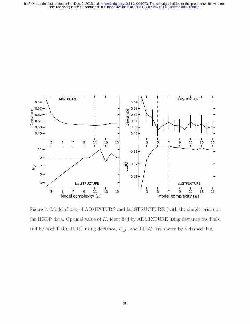
3 5 7 9 11 13 15

0.49

0.50

0.51

0.52

0.53

0.54

De

via

nce

3 5 7 9 11 13 15

0.49

0.50

0.51

0.52

0.53

0.54

De

via

nce

3 5 7 9 11 13 15

3

5

7

9

11

K∅∁

3 5 7 9 11 13 15

-0.93

-0.92

-0.91

LLB

O

Model complexity (K) Model complexity (K)

ADMIXTURE fastSTRUCTURE

fastSTRUCTURE fastSTRUCTURE

Figure 7: Model choice of ADMIXTURE and fastSTRUCTURE (with the simple prior) on

the HGDP data. Optimal value of K, identified by ADMIXTURE using deviance residuals,

and by fastSTRUCTURE using deviance, K∅∁ , and LLBO, are shown by a dashed line.

39


http://dx.doi.org/10.1101/001073


K∗ E=7

San

Mb

uti

Bia

kaYo

rub

aM

and

enka

Ban

tuM

ozab

ite

Bed

ouin

Pale

stin

ian

Dru

ze

Ad

ygei

Sar

din

ian

Tusc

anIt

alia

nFr

ench

Orc

adia

nB

asq

ue

Ru

ssia

n

Mak

ran

i

Bal

och

i

Bra

hu

i

Kal

ash

Bu

rush

o

Path

an

Sin

dh

i

Haz

ara

Uyg

ur

Yaku

tM

ong

ola Tu

Xib

oO

roq

enH

ezh

enD

aur

Jap

anes

e

Yizu

Nax

iTu

jia

Han

Sh

eM

iaoz

uD

aiLa

hu

Cam

bod

ian

Mel

anes

ian

Pap

uan

May

a

Pim

aC

olom

bia

nK

arit

ian

aS

uru

i

K∗ ∅∁=9

fast

ST

RU

CT

UR

E

Africa Mid.East Europe C.S.Asia E.AsiaOceania

America

K∗ cv=5

K∗ cv=11

AD

MIX

TU

RE

Figure 8: Ancestry proportions inferred by ADMIXTURE and fastSTRUCTURE (with the

simple prior) at the optimal choice of K identified by relevant metrics for each algorithm.

Notably, the admixture proportions at K = K∗E and K = K∗

∅∁ are quite similar, with

estimates in the latter case identifying the Kalash and Karitiana as additional separate

groups that share very little ancestry with the remaining populations.

40


http://dx.doi.org/10.1101/001073


Documents

Variational Inference of Population Structure in Large … · Variational methods, originally used for approximating intractable integrals, have been used for a wide variety of applications