Valuation of Urban Air Pollution: A Case Study of …€¦ · Valuation of Urban Air Pollution: A Case Study of Kanpur City in India ... Gas (CNG) in many cities; changes in the mode

SANDEE Working Paper No. 17-06 I

USHA GUPTA

Bhim Rao Ambedkar College, University of DelhiDelhi, India

SANDEE Working Paper No. 17-06

May 2006

South Asian Network for Development and Environmental Economics (SANDEE)PO Box 8975, EPC 1056

Kathmandu, Nepal

Valuation of Urban Air Pollution:A Case Study of Kanpur City in India

II SANDEE Working Paper No. 17-06

Published by the South Asian Network for Development and Environmental Economics(SANDEE)PO Box 8975, EPC 1056 Kathmandu, Nepal.Telephone: 977-1-552 8761, 552 6391 Fax: 977-1-553 6786

SANDEE research reports are the output of research projects supported by the SouthAsian Network for Development and Environmental Economics. The reports have beenpeer reviewed and edited. A summary of the findings of SANDEE reports are alsoavailable as SANDEE Policy Briefs.

National Library of Nepal Catalogue Service:

Usha Gupta

Valuation of Urban Air Pollution: A Case Study of Kanpur City in India

(SANDEE Working Papers, ISSN 1893-1891; 2006 - WP 17)

ISBN: 99946-810-5-2

Key words:

1. Air Pollution

2. Health Damages

3. Mitigating Activities

4. Health-diary

5. Panel Data

6. Health Production Function.

The views expressed in this publication are those of the author and do not necessarilyrepresent those of the South Asian Network for Development and EnvironmentalEconomics or its sponsors unless otherwise stated.

SANDEE Working Paper No. 17-06 III

The South Asian Network for Development andEnvironmental Economics

The South Asian Network for Development and Environmental Economics (SANDEE)is a regional network that brings together analysts from different countries in SouthAsia to address environment-development problems. SANDEE’s activities includeresearch support, training, and information dissemination. SANDEE is supported bycont r ibut ions f rom in terna t ional donors and i t s members . P lease seewww.sandeeonline.org for further information about SANDEE.

SANDEE is financially supported by International Development Research Centre(IDRC), The Ford Foundation, Swedish International Development CooperationAgency (SIDA) and Norwegian Agency for Development Cooperation (NORAD).

Technical EditorPriya Shyamsundar

Priya Shyamsundar

English EditorCarmen Wickramagamage

Comments should be sent to Usha Gupta, Bhim Rao Ambedkar College, University ofDelhi , India, Email : [email protected]

IV SANDEE Working Paper No. 17-06

SANDEE Working Paper No. 17-06 V

TABLE OF CONTENTS

1. INTRODUCTION 1

2. AIR POLLUTION AND HEALTH EFFECTS 3

3. STUDY AREA 5

4. DATA SOURCES AND SURVEY DESIGN 6

5. METHODOLOGY 9

5.1 ESTIMATING THE HOUSEHOLD PRODUCTION FUNCTION 11

5.2 DEMAND FOR MITIGATING ACTIVITY 11

5.3 EMPIRICAL SPECIFICATION 13

6. RESULTS 14

6.1 WELFARE GAIN 15

6.2 OPPORTUNITY COST OF THE REDUCTION IN WORKDAYS 16

LOST

6.3 REDUCTION IN MITIGATING ACTIVITIES (MEDICAL 16

EXPENDITURE)

7. CONCLUSION AND POLICY IMPLICATIONS 17

8. ACKNOWLEDGEMENTS 18

REFERENCES 19

TABLES AND FIGURES 22

APPENDIX A 29

APPENDIX B 32

APPENDIX C 33

APPENDIX D 39

LIST OF TABLES

Table 1 : Estimated Loads of Pollutants of Different Vehicles in Kanpur 22

Table 2 : Point Source Emissions in (kg. / hr.) 22

Table 3 : Emissions from Domestic Fuels 23

Table 4 : Source Distribution of PM10 (RSPM) in Various Areas of Kanpur 23

Table 5 : Distribution of Households in the Sample 23

Table 6 : Summary Information for the Household Survey 24

VI SANDEE Working Paper No. 17-06

LIST OF FIGURES

Figure 1 : Air Pollution in Different Cities in India 27

Figure 2 : Air Quality in Kanpur 27

Figure 3 : Weekly Average of RSPM (µg/m3) for the Stated 18 Weeks 28

Table 7 : Descriptive Statistics of Variables Used in Estimation 24

Table 8 : Poisson Equations of Workdays Lost (H) 25

Table 9 : Tobit Equations of Mitigating Activities (M) Left Censored (0) 26

Table 10 : Negative Bionomial Equation of Workday Lost (H) 30

SANDEE Working Paper No. 17-06 VII

Abstract

This study estimates the monetary benefits to individuals from health damages avoidedas a result on reductions in air pollution in the urban industrial city of Kanpur in India.A notable feature of this study is that it uses data from weekly health-diaries collectedfor three seasons. For measuring monetary benefits, the study considers two majorcomponents of health cost — the loss in wages due to workdays lost and the expenditureincurred on mitigating activities. The study estimates that a representative individualfrom Kanpur would gain Rs 165 per year if air pollution was reduced to a safe level.The extrapolated annual benefits for the entire population in the city are Rs 213 million.

Key words: Air Pollution, Health Damages, Mitigating Activities, Health-diary, PanelData, Health Production Function.

VIII SANDEE Working Paper No. 17-06

SANDEE Working Paper No. 17-06 1

Valuation of Urban Air Pollution: A Case Studyof Kanpur City in India

Usha Gupta

1. Introduction

While large-scale industrialization increases the production of material goods andurbanization creates mega cities, the ill effects of these activities are reflected in theform of various environmental problems. One such problem is the deterioration ofurban air quality in India and other developing countries. The main contributing factorsto air pollution are the overwhelming concentration of vehicles, poor transportinfrastructure and the establishment of industries in urban agglomerations.Epidemiological studies have shown that there is a significant association between theconcentration of air pollutants and adverse health impacts (Ostro, et al., 1995; MJA,2004). Air pollution contributes to illnesses like eye irritation, asthma, bronchitis,etc., which invariably reduce efficiency at work.

Among the different types of air pollutants, suspended particulate matter (SPM),especially Respirable Suspended Particulate Matter (RSPM), is recognized as the mostimportant in terms of health effects.1 It can penetrate deep into the respiratory tractand cause an increase in cardiac respiratory illnesses, even mortality; contribute todaily prevalence of respiratory symptoms; and decrease pulmonary lung function inchildren and adults. These illnesses cause functional limitations as reflected by loss ofworkdays, absence from school, restrictive activity days, and an increase in the visitsto doctor and emergency rooms for aggravated asthma and other respiratory illnesses(COMEAP, 1998; M.El-Fadel and M. Masood, 2000; CEAP, 2004). The importanceof the link between air pollution and health is underscored in a study by Pope, et al.,(2002), who show that residents who live in an area, in California, that is severelyimpacted by particulate air pollution are at a greater risk of lung cancer at a ratecomparable to non-smokers exposed to second-hand smoke. It is observed in thisstudy that there is an excess risk of approximately 16 percent dying from lung cancerdue to fine particulate air pollution.

Given the significant impact of air pollution on health, it is important that it be explicitlyaccounted for in economic planning. This requires, however, economic valuation ofthe benefits of remedial measures taken to reduce air pollution impacts. Sinceenvironmental attributes have the characteristics of public goods, market prices thatallow us to estimate the benefits of decreasing air pollution are unavailable. However,using non-market valuation techniques, the benefits of air pollution reduction can be

1 Well known air pollutants are total suspended particles (TSP), nitrogen oxides (NOx), sulphurdioxide (SO2) and respirable suspended particulate matter (RSPM). Particulate Matter (PM)with an aerodynamic diameter of 10pm or less, known as RSPM or PM10, remains in theatmosphere for longer periods because of its low settling velocity (World Bank, TechnicalPaper No.737, 1997).

2 SANDEE Working Paper No. 17-06

evaluated. Such economic valuation will enable policy makers to compare benefits ofreduced air pollution to the cost of air pollution abatement and to provide inputs fordesigning policies for air quality improvement and its control mechanism. In developingcountries, however, very few studies of this sort have been conducted so far. Theproposed study is an attempt to examine air quality improvements and to estimate itshealth benefits to the people of Kanpur in India.

Kanpur is an important center for trade and commerce in Uttar Pradesh. However, inrecent years, Kanpur has acquired notoriety as the second most polluted industrialcity in India after Ahmedabad in terms of RSPM concentration, followed by Kolkata,Jaipur, Solapur, Hyderabad, Mumbai, Bangalore and Kochi.2 There is evidence of ahigh percentage of chronic illnesses like asthma, BP, Tuberculosis, heart disease, etc.,and this has created widespread concern in Kanpur. One of the main sources of airpollution is the industry associated with textiles, heavy engineering and tanneries. Thecity is also a major distribution center for finished leather products, textiles and fertilizer.Moreover, lack of opportunities for gainful employment in rural areas has led to anever-increasing migration of poor families to the urban city of Kanpur resulting in thegrowth of urban slum clusters and an increase in urban poverty. This has exerted extrapressure on the environmental resources of the city.

In many urban cities of India the pollution levels are much above the international anddomestic safety standards. Consequently, in recent years there has been a strongmovement to introduce environmental policy changes that can improve air quality.Notable among these policy changes are the recent introduction of Compressed NaturalGas (CNG) in many cities; changes in the mode of transportation from road to rail inDelhi and Kolkata; and relocation of industries in some urban areas. All of theseefforts result in significant costs to industries, commuters and the government. Suchcosts need to be justified on economic grounds.

In response to the obvious problem of air pollution in the city of Kanpur, in the year1997-98 the Central Pollution Control Board (CPCB) developed an EnvironmentalManagement Plan (EMP) for Kanpur with a strong focus on air pollution reduction.As a first step, the city was mapped in terms of land use, location of industries,environmental resource areas, housing quality, water supply, drainage, surface andground water quality, air quality, solid waste collection status and environmentalhotspots. To reduce air pollution, the plan recommended an improvement in the city’sroad network through the construction of more road corridors and through theregulation of traffic to decongest the residential and market areas. It also proposedthe realignment of the Meter-Gauge (MG) Rail Track along the Broad Gauge line.3 Infact, the plan recommends a wide range of measures involving very high expenditure toimprove environmental quality. These new costly measures underscore the need toestimate the economic benefits of improved air quality in the city.

2 See Report of the Expert Committee on Auto Fuel Policy, R. A. Mashelkar (August 2002).3 The MG Rail Track has been identified as a major source of air pollution. Whenever the train

passes through this track, the level of air pollution rises significantly due to traffic congestionat the crossings, which are seventeen in number.


To estimate the environmental benefits of reduced urban air pollution in Kanpur, thisstudy uses a variant of what is referred to as a household health production functionmodel (HHPF). Essentially, this means that data on expenditure incurred by individualsto lessen the effects of air pollution is taken into account in estimating the health impactsof changes in air quality. The overall impact of air pollution on health is estimated asthe sum of mitigating expenditure incurred and the sick days lost as a result of sicknessthat can be attributed to pollution. A noteworthy feature of this study is the use ofhealth diary data to estimate welfare gains to working individuals from reduced airpollution. To examine the impact of seasonal variations on health, the diary data hasbeen collected for three seasons (winter, summer and monsoon) over an eighteen-week period.

This paper is organized as follows. Section II reviews existing research on air pollutionand its health impacts; Section III describes the study area; Section IV gives details ofdata sources and the design of the household survey; Section V presents methodology;Section VI provides the descriptive statistics of variables used in estimation; SectionVII presents the estimates of Poisson and Tobit models and the welfare gains; SectionVIII gives the conclusions and discusses some policy implications.

2. Air Pollution and Health Effects

There is a vast global literature on air pollution and health. Most of these existingstudies on air pollution and health are based on the physical linkage approach, wherea dose response function is estimated in order to observe the relationship betweenhuman health and air pollution. This relationship is also called the damage function andlinks air pollution to mortality or morbidity. Well-known among these studies is workby Ostro (1983; 1987), who estimated dose response functions to observe the effectof air pollutants on morbidity and showed that particulates affect both restricted activitydays (RAD) and work loss days (WLD). His work suggests that a one percent increasein particulate matter will increase WLD by about 0.5% and RAD by 0.4%.

Another interesting study relevant to this research is by Chestnut, et al., (1997) whocompare the results of various studies on health effects and economic valuationconducted in Bangkok, Thailand, concerning particulate matter air pollution. The studycompares the willingness to pay for air quality improvements between Bangkok andthe US4 and finds that Bangkok residents are willing to pay a higher share of theirincome to protect their health. A tentative but plausible explanation given here is thathealth is seen as a basic necessity on par with food and shelter.

Using 1991-92 data for the Republic of China (Taiwan), Alberini and Krupnick (2000)compare the cost of illness (COI) and willingness to pay (WTP) estimates related tohealth damages from minor respiratory symptoms associated with air pollution. This

4 The mean WTP value for a symptom day in Bangkok is $16 (a sample of 141 adults) while in theU S it is $11 (selected estimates from US studies). For RAD, these values are $30 and $26respectively.


study shows that the ratio of WTP to COI ranges from 1.61 to 2.26 depending onpollution levels. These ratios are similar to those obtained for the U S in previousstudies, despite differences in geographical and socio-economic characteristics betweenthe two countries.

Another relevant study from the developing world is one by M. El-Fadel and Masood(2000) who estimate the economic values of mortality and morbidity for Lebaneseurban areas. The total emergency visits avoided due to 10 µg / m3 reduction in PM10are reported to be in the range of 609 - 25,578. The corresponding total economicbenefit (estimated by using the human capital approach) is reported to be MUS$ 0.05-1.9 per year.

In a recent study in India, Murty, et al., (2003) use household data that relates to arecall period of six months. The study analyzes the impact of higher levels of SuspendedParticulate Matter (SPM) in the Indian metropolitan cities of Delhi and Kolkata. Usingthe three stage least square method, a system of simultaneous equations consisting ofthe health production function and the demand functions for mitigating and avertingactivities are estimated. The study reveals that the annual marginal benefits to a typicalhousehold is Rs 2086 in Delhi and Rs 950 in Kolkata if the level of SPM is reducedfrom the current average level to the prescribed safe level.

Two other notable Indian studies that estimate benefits of air pollution reduction are astudy by Kumar and Rao (2001) in Haryana, India, and Cropper, et al., (1997) usingdata from Delhi. Kumar and Rao (2001) estimate a dose-response function to measurethe economic benefits of improved air quality in the residential complex (consisting2400 families) of the Panipat Thermal Power Station. Based on an earlier model byGerking and Stanley (1986), they calculate the monetary costs from morbidity due tohigher levels of PM10 emission. This study suggests that for a sixty-seven percentreduction in the level of ambient mean PM10 concentration, which is required to meetNational and World Health Organization (WHO) standards, households in Panipat,India are willing to pay on the average an amount that ranges from Rs 12 to Rs 53 permonth.

Cropper, et al., (1997) examine the dose-response relationship between a rise in airpollution (in terms of total suspended particulates) and an increase in mortality rates inDelhi, India. While the monetary benefits to the households from reduced air pollutionare not estimated in this study, they find that 2.3% of non-trauma deaths in Delhi arerelated to a 100 µg / m3 increase in Total Suspended Particulate Matter (TSPM). Theimpact of TSPM non-trauma deaths is found to be statistically significant for the agegroups of 5-14 to 45-65 years in Delhi.

All of these studies suggest that there are significant benefits to be derived from reducingair pollution in urban India. This paper examines similar issues in Kanpur.


3. Study Area

Kanpur is the largest and most populous industrial city in the state of Uttar Pradesh inIndia. According to the 2001 Population Census Data in India, the population ofKanpur was 2.7 million with the annual growth rate at 2.47 percent and populationdensity at 6800 Persons / sq.km. The percentage of the workforce involved in theprimary, industrial and service sectors are 4 per cent, 31 per cent and 65 per centrespectively.

The urban limits of Kanpur Nagar are spread over an area of 215 square kms. Thecity is bound between two rivers, the Ganges in the North and the river Pandu in thesouth. It is a linear city developed between rivers and the railway lines. Kanpur isfamous for its cotton, woolen and leather industries. Kanpur was once known as the“Manchester of Northern India” but over the years has unfortunately gained notorietyas a dirty and polluted city. All the important industries such as textiles, heavyengineering, tanneries, fertilizer and leather are situated in the heart of the city withresidential areas on either side. Besides industrial production, the city is a majordistribution centre for finished leather products, textiles and fertilizer.

Air pollution in the core areas of Kanpur is five to six times higher than prescribedstandards and the level of RSPM (PM10) in residential and industrial areas of the cityexceeds the National Ambient Air Quality Standards by 200 percent (NAAQS,Appendix B). Figure 1 compares the annual RSPM level in the various cities in Indiain the year 2000. Kanpur turns out to be the most polluted in terms of residential airpollution, on par with Ahmadabad, but holds second position when it comes to industrialair pollution.

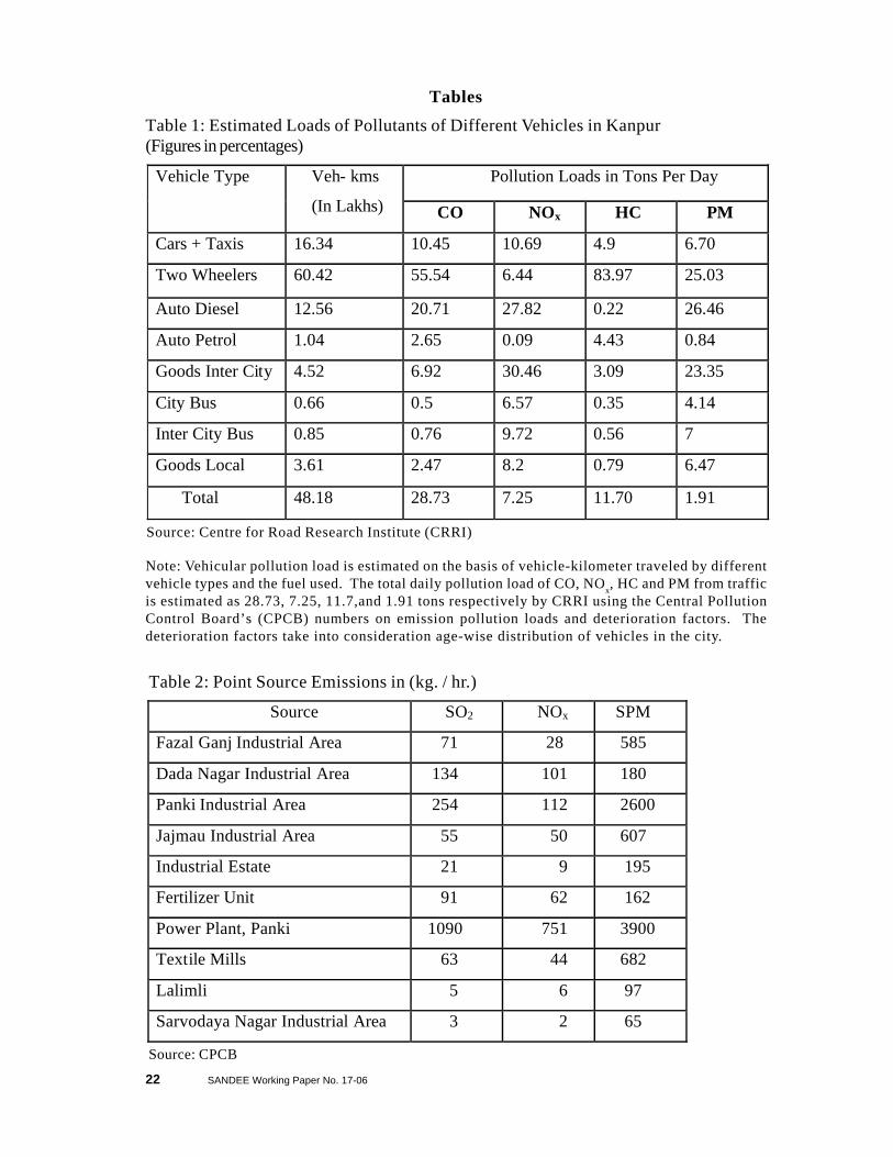
Overwhelming industrial activity and the fleet of mixed vehicles are the two maincontributing factors for urban air pollution in the city. Badly maintained roads, a mixedtraffic pattern, and, road encroachment aggravate the impact of vehicular pollution inKanpur. There are about 0.2 million petrol / diesel driven vehicles that ply the roads inKanpur contributing about 142 MT of pollutants per day. Diesel driven temposconstitute a major portion of the public transport system, causing heavy noise pollutionas well as smoke emissions in the city. The Meter Gauge railway track, along theresidential areas in the western part of city, has seventeen intersection points, knownas Goumti. Whenever the train passes through this track, the level of air pollution goesup by 6 to 8 times due to the increased idling time of vehicles and traffic congestion(CPCB). Table 1 gives the pollution loads of different vehicles in Kanpur. It showsthat diesel autos emit the maximum amount of particulate matter (PM) in the city followedby two-wheelers and the intercity movement of goods by road.

The emissions of pollutants such as SO2, NOx and SPM from industrial sources in eachof the industrial areas and point source emissions in the city are shown in Table 2. Thistable shows that emissions of SO2, NO2 and SPM from industrial areas such as thePanki power plant, the industrial area and Dada Nagar are quite high. Fly ash generatedby the Panki power plant in the Northern part of Kanpur is also one of the majorsources of air pollution in the city.


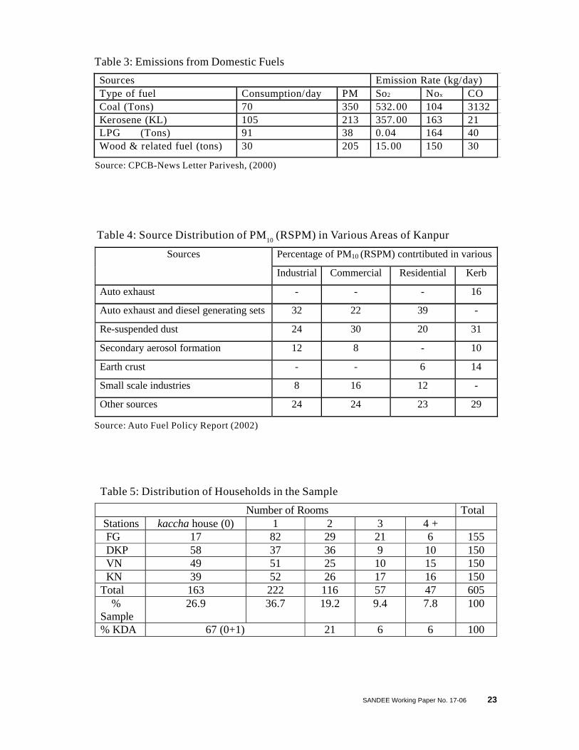
Another source of air pollution in Kanpur is domestic fuel. Use of coal, wood, cow-dung, etc., in the slum settlements and low-income group (LIG) colonies along therailway yard generate localized smoke problems, which affect visibility and cause eyeirritation. The estimated pollution load from household fuel is 5.5 MT/Day. Due tostable wind conditions the problem becomes even more severe during winter. Data onemission loads from domestic or household sources are given in Table 3.

The National Environment Energy Research Institute (NEERI) conducted pollutionsource inventory surveys in the city of Kanpur and submitted its report in July, 2002(Table 4). NEERI data shows that the highest amount of RSPM is generated by autoexhaust and diesel power generating sets (39%), followed by re-suspended dust (31%)and industrial and other sources (25 to 40%).

Figure 2 provides a geographic sense of the distribution of air pollution. This graph,obtained from the report of Environmental Management Plan (2000) of Kanpur,provides a vivid picture of the condition of air quality in Kanpur. It shows that theentire central part of the city, which is both densely populated and has business centres,is the highly polluted air quality zone. About 60 percent of the geographical area of thecity has air pollution problems. It is not surprising that the city is considered one of thehot spots in the country with regard to air pollution.

4. Data Sources and Survey Design

The data for the present study was obtained through both household surveys and sec-ondary sources. In October 2003, a pilot survey was conducted to assess the impactof air pollution on the health of residential households in certain randomly chosen ar-eas of urban Kanpur. The sampling frame was constructed based on the Kanpur De-velopment Authority’s classification of households. The main survey commenced inJanuary 2004 and was completed in September 2004. The primary data were col-lected by administering a questionnaire (see Appendix C) through a face-to-face in-terview with the head or any other working member of the household. The secondarydata, relating to the ambient air quality (RSPM) and weather conditions (temperatureand humidity), was collected from the publications of the Central Pollution ControlBoard (CPCB), U P, Pollution Control Board (UPPCB), and the Department of Me-teorology (Chandra Shekhar Azad University of Agriculture, Kanpur).

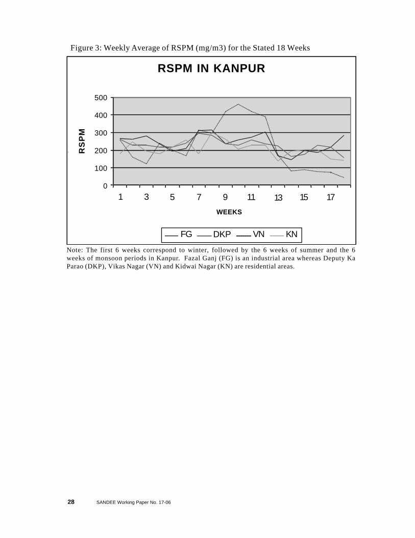
Monitoring of RSPM in Kanpur by the National Environment and Energy ResearchInstitute (NEERI), the Central Pollution Control Board (CPCB) and the Uttar PradeshPollution Control Board (UPPCB) started in the year 2000. The RSPM data for thepresent study was collected from the records of the CPCB and the UPPCB (from fourstations), and covers eighteen weeks over three seasons. The three stations moni-tored by the UPPCB include residential areas (Deputy Ka Parao, Vikas Nagar, andKidwai Nagar) while the one monitored by the CPCB is an industrial area (Fazal Ganj)though it is also surrounded by a large residential area. Figure 3 shows season-wisethe weekly average of RSPM (mg/m3) at the four monitoring stations in Kanpur. Itshows that the level of air pollution is higher than the National Ambient Air Quality


Standards (NAAQS) at all the locations5. Vikas Nagar registers wild fluctuations inthe level of RSPM (295 and 463 ìg/m3 respectively are the minimum and maximumlevels of RSPM) during summer whereas during the monsoon and winter seasons it isas low as 42.5 and 122 ìg/m3 (minimum) respectively. The other locations too registerfluctuations in the level of RSPM during the three seasons but the volatility is not ashigh. The reasons for these fluctuations are explained by meteorological and weatherconditions.

Different seasons play an important role in determining the ambient concentrations ofair pollutants. During the monsoon months (July, August and September), air of oceanicorigin causes increased humidity, cloudiness and precipitation. Frequent rains washaway the airborne particulates and other pollutants that are generated and dispersedfrom different sources. Hence, the period from July to September is supposedly cleanerin terms of RSPM and all the locations register a low level of RSPM during the monsoonperiod. Winter months (November to February), on the other hand, are dominatedby high pressure causing increased atmospheric stability, which allows for both lowcirculation and stagnant air masses that result in the accumulation of pollutants in theatmosphere. Thus, a more stable atmosphere and slow dispersion of pollutants helpbuild up pollutants in the vicinity of pollution sources. The strong and medium windsduring summer (April to June) create turbulent conditions. Local disturbances in theenvironment cause frequent dust storms and a hazy atmosphere, which build up highlevels of particulate matter in the ambient air, mostly soil-borne particles.

Health data were collected through a household survey. The sampling procedure usedfor the household survey was based on a two-stage stratification—air pollutionmonitoring stations and the type of accommodation. For the first stage of stratification,we located air pollution monitoring stations in the city. Then, using a meter taxi, anarea of one-kilometer radius was marked around each station. During our surveyperiod, there were four functional monitoring stations. Out of these, the one at VikasNagar (VN) was maintained by CPCB while the rest at Fazal Ganj (FG), Deputy kaParao (DKP) and Kidwai Nagar (KN) were managed by UPPCB. We drew a sampleof households that contained almost equal numbers of households from each monitoringstation area.

The second stage of stratification followed Kanpur Development Authority’s (KDA)classification of households based on “types of accommodations”, which broadlyreflects economic status. According to KDA, 67 percent of the total population livesin a kaccha house, single room or a portion thereof; 21 percent in two-room dwellings;and 12 percent in three or more rooms’ dwellings. The sample households of aparticular station are distributed across household types in proportion to the numberof households in each type. All the households in the marked area around each stationwere allotted a serial number and random numbers generated by the computer (thelottery system) were used to identify the households to be included in the sample.

5 Safe levels as prescribed by NAAQS are the levels of air quality, with an adequatemargin of safety, which are necessary to protect public health, property andvegetation.


Our final sample consisted of 222 and 163 households residing respectively in one-room and kaccha houses representing households belonging to the poorest section ofthe society; 116 households living in two-roomed dwellings, representing the lowermiddle class category; and 57 and 47 households residing in three- and more than fourroomed houses respectively and considered to be of higher income levels. Table 5shows the distribution of sampled households across the four monitoring stationsaccording to the size of dwellings.

The survey questionnaire used for the household survey had four main sections withdetailed subsections to facilitate the collection of relevant data on key variables. Thus,sections 1, 2 and 4 covered various socio-economic and demographic features suchas religion, family background, age and sex composition of household members, levelof education, marital status, occupation and the size of the accommodation / house.Section 3 provided data on the current health status (symptoms of acute illnesses linkedto air pollution exposure) and mitigating and averting activities adopted by all themembers in a household for a recall period of one week. Its sub-sections containedinformation on individuals’ past health stock (chronic diseases), their habits that affecthealth in general and the general awareness of households about the illnesses that occurdue to air pollution.

To assess indoor air quality and exposure to indoor air pollution, information on theuse of home A.C., cooking gas, exhaust fan or chimney, room heater, home affectedby road dust, dampness, mosquito repellent, etc., were also collected. Data on drinkingwater quality was obtained to account for water-borne illnesses.

In order to collect data on gross annual income, different income brackets were offeredto the respondents to select their respective range of income. Data on an alternativemeasure of wealth of households/individuals in the form of average annual expenditureand inventory of durable consumer items were also collected to crosscheck the incomelevels.

A unique feature of this study is the Weekly Health Diary, which sought to capture theimpact of seasonal variations on health. The diary data was collected for eighteenweeks (six weeks in each season—summer, winter and monsoon) covering workingindividuals from the targeted households. Trained enumerators visited each of thesehouseholds, every week, in each season, to fill the diary data on mitigating activitiesand the workdays lost due to illness. The seasonal phases to which the diary databelongs are: winter season (Jan.’04—Feb.’04); summer season (May ’04%June ’04)and the monsoon season (July ’04—Sept ’04).

With the 18 weeks of health diary data and a total of 3122 household members(consisting of both children and adults), the existing data set results in a panel containing58,196 observations (3122 x 18). The present study focused on working individuals.The sample included 863 working individuals. However, only 815 working memberscould be taken into consideration on the basis of availability of full information.


Table 6 presents summary information on the household survey. Most households inthe city report nuclear families as is indicated by the family size (5.2) and the numberof married persons. Data on religion shows that most households are Hindu. Onaverage, individuals have six years of education. Eighteen percent of individuals in thesample reported to be smokers.

Coal is used by 28.8 percent of the population for the purposes of cooking and spaceheating. It generates localized smoke that causes invisibility in the concerned areas(particularly, in slum settlement colonies) as well as indoor air pollution. Thirty twopercent households keep indoor plants, particularly Basil plant for religious andmedicinal reasons and other plants for decorative purposes. Green plants in earthenpots are watered regularly, which add to the dampness and affect health of householdsadversely. Chronic patients are 10.2 percent, which represent the poor health stockof the households.

5. Methodology

We use the household health production function model to estimate the economicbenefits from reduced morbidity due to reduction in air pollution in Kanpur city. Thehousehold health production function and the demand function for mitigating activities6

that are implicit in the utility maximizing behavior of an individual are based on Freeman(1993) and derived as follows:

An individual’s utility function, health production function and the budget constraintmay be defined as

( )QHLXUU ,,,= (1)where, X is the consumption of marketed goods, L denotes leisure time available perperiod to an individual, H represents the work days lost per week due to air pollutioninduced sickness and Q shows the level of ambient air pollution. The individual derivesutility from the consumption of X and L, while H and Q result in disutility.

An individual produces good health by combining mitigating activities with the givenlevel of air pollution (Q) given his health status and other socio-economic characteristics.

The household health production function can be written as

( )ZQMHH ,,= (2)where,H: number of work days lostM: mitigating activitiesQ: level of ambient air pollutionZ: a vector of other health characteristics of an individual

6 The estimated model does not include averting activities because the survey data revealsthat people in Kanpur do not adopt averting activities (such as a.c. car, staying indoors,using heater, mask, diverting to cleaner route, etc.,) to avoid exposure to air pollution.


H could also represent the individual’s health status or number of days of illness.Mitigating activities (M) include the individual’s demand for medicines, hospitalization,pathological tests, doctor’s consultation and travel to doctor’s clinic. The other healthcharacteristics (Z) of an individual are the history of chronic illness, food and otherhabits. The model assumes that individuals could maintain a given health status evenwith higher ambient air pollution through the choice of mitigating activities in the market.It means that there are substitution possibilities between mitigating activities and theambient air quality.

An individual’s budget constraint can be specified as:

( ) MPXHLTwYI M+=−−+= (3)where, Y is non-wage income; w is wage rate; (T-L-H) is time spent at work (T is totaltime); PM is the price per unit of mitigating activity.

Given the pollution level (Q), prices of mitigating activities (PM), wage rate (w), income(I) and other exogenous variables, individuals maximize (1) with respect to X, M, andL given the budget constraint (3). By solving the following problem,

( )[ ]MPXHLTwYQHLXUMaxG M−−−−++= λ),,,( (4)

where λ is the Lagrange multiplier.

We obtain the individual’s demand function for mitigating activities, and the marginalwillingness to pay function for air quality improvement (MWP) as7:

( )ZXQHPMM m ,,,,= (5)

( ) λδδδδ //.//./. dQdHHuQMPdQdHwMWTP M ++= (6)

7 See Freeman (1993)

This expression in (6) shows that the MWTP for health benefits from the reduction inpollution is the sum of observable reductions in the cost of illness, cost of mitigatingand the monetary equivalent of disutility of illness. The estimation of MWTP requiresthe estimation of the health production function (2) and the demand function formitigating activities (5) simultaneously. Alternatively, a reduced form dose-responsefunction with health as a function of pollution and other variables can be estimated.This can be combined with the estimated demand for mitigating behaviour and wageinformation to obtain a lower bound for (6) (Freeman 1993). This is a lower boundestimate because it does not take into account disutility from sickness (the last expressionin (6)).


5.1 Estimating the Household Production Function

For estimation purposes, there are two salient features of the present data set thatneed to be taken into account: (i) the dependent variable is a count of the total numberof the workdays lost by an individual, due to air pollution induced illnesses, in a givenweek during the three seasons; (ii) there are repeated observations for the sameindividuals. Thus, this data forms a combined time-series cross-section panel.

The occurrence of morbidity due to air pollution is not a continuous phenomenon andis discrete in nature. The data collected from the survey provides count events ofmorbidity, where there are zeros for several observations. In this case, the applicationof the Poisson regression model is appropriate because it accounts for thepreponderance of zeros and the small values and the discrete nature of the dependentvariable while least square and the linear models do not take into consideration thesecharacteristics. Thus, for estimating the household health production function, we usea Poisson regression model.

( ) !// ity

itititit yexyYprob itit µµ −== yit = 0,1,2,…………. (7)

The resulting regression model is nonlinear in parameters. By taking the natural log ofequation (7) we obtain the following regression model which is linear in parameters,

ln =itµ sitsititi XXX βββα ++++ .......2211 iα + b2 X2it + b3 X3it +———+ bS XSit (8)

However, it is noted that in practice the Poisson regression model is restrictive in manyways. Firstly, it is based on the assumption that events occur independently over time.The independence assumption may break down, as there may be a form of dynamicdependence between the occurrences of successive events. For example, the prioroccurrence of an event, such as workdays lost due to air pollution induced illness, mayincrease the probability of a subsequent occurrence of the same or similar event.Secondly, the assumption that the conditional mean and variance of yi, given Xi areequal, may also be too strong and hence fail to account for over dispersion (the varianceexceeds the mean). This restriction may produce small estimated standard errors ofthe estimated β. An alternative to scaling the standard errors is to apply the negativebinomial distribution, which is attempted in Appendix A.

5.2 Demand for Mitigating Activity

An important characteristic of the survey data on mitigating activities is that it hasseveral observations where the medical expenditure is zero. This feature of the datadestroys the linearity assumption; hence the application of the least squares method isinappropriate. Also the continuous density to explain the conditional distribution ofmedical expenditure, given income, cannot be used because a continuous density is


inconsistent with the fact that the data on mitigating expenditures contains severalobservations at zero.8 Therefore, to estimate the demand for mitigating activities, we use a Tobitmodel.

iitit uxM ++= βα if RHS >0 (9) = 0 otherwise

where, Mit refers to the probability of the ith household incurring positive mitigating expenditureat time t, and xit denotes a vector of individual characteristics, such as income, age and education,pollution parameters, weather conditions, etc.

In panel data there are two approaches of estimating the above functions (the HouseholdHealth Production and the Demand Function for mitigating activities), that is, the fixedeffects and random effects models. Panel data contain individual specific heterogeneity,which arises due to unobserved or imperfectly observed differences in individualcharacteristic / behavior. To handle this heterogeneity, in the fixed effects estimationeach individual has its own (fixed) intercept value, that is, in all there are N such valuesfor N individuals. The individual intercept captures the combined effect of bothobservable and unobservable time invariant variables (such as age, income, attitudeetc.) but does not identify the impact of such time invariant variables separately.Therefore, in the estimation of fixed effects model we obtain only the values of timevariant variables (such as weather conditions etc).

On the other hand in the random effects model the intercept ái, represents a commonmean value for the all the (cross-sectional) intercepts and the individual specific errorcomponent represents the (random) deviation of individual intercept from this meanvalue. Thus, the individual differences in the intercept values of each person arereflected in the composite error term ? ita in the random effect model (equ.8). Thecomposite error term consists of two components, ei, which is the cross-section orindividual specific error component, and uit, which is combined time series and cross-section error component. The random effects model assumes that error terms arenormally distributed. The individual error components are not correlated with eachother and are not auto correlated across both cross-section and time series units.

),0(~ 2εσε Ni

),0(~ 2uit Nu σ

0)( =itiuE ε 0)( =jiE εε ( )ji ≠

0)()()( === jsitjtitisit uuEuuEuuE ( )stji ≠≠ ; .

The individual error component, ei, is not directly observable so it is termed as latentor unobservable variable.

8 T Amemiya (1984), “Tobit Models: A Survey.”


5.3 Empirical Specification

Empirically, we estimate the following two reduced form equations consisting of thehousehold health production function and the demand function for mitigating activitiesto estimate the marginal effect of pollution on H and M. We use the random effectspanel data regression model to estimate both these equations.9

The dependent variables used in the equation are: Work Lost Days (H): H represents the number of workdays lost per person perweek due to diseases / symptoms associated with air pollution.Mitigating Activities (M): Mitigating activities (M) include expenses incurred as a resultof air pollution related diseases. These expenditures include costs of medicines,doctor’s fees, diagnostic tests, hospitalization, travel to doctor’s clinic, etc., per person,per week.

The independent variables that affect the health production function and mitigatingactivities are:Respirable Particulate Matter (PM10): This is the average of the maximum twice-weeklyvalues of RSPM (PM10) measured in µg/m3 10. RSPM remains in the atmosphere forlonger periods because of its low settling velocity. It can penetrate deeply into therespiratory tract and cause respiratory illnesses in humans.

The Variation in Temperature (DTEMP): It is the difference of the average values ofdaily maximum and minimum temperatures. The temperature swings cause acute illnesseslike coughing, cold, fever, etc.Maximum Ambient Temperature (TMAX): It is the weekly average of daily maximumambient temperature.

υββββββββββββββα

+++++++++++++++=

heartTBBPasthmabcj

ageagerhwindSONOtdtemprspmH xi

1413121110

29876254321 minmax

ϖδδδδδδδδδδδδδδγ

+++++++++++++++=

heartTBBPasthmabcj

ageagerhwindSONOtdtemprspmM xi

1413121110

29876254321 minmax

9 The Hausman test for choosing between the fixed and random effects models is in favor ofthe random effects model in the estimation of Poisson regression model for work days lost.The Tobit model only estimates the random effects model.

10 In Kanpur the values of pollutants such as RSPM, NOx , SO2,, etc. are recorded during twodays in each week, with three readings taken on each day. We have taken the maximum valueof each day ’s readings and averaged them over the two days of readings to find the value foreach week.

Nitrogen Oxides (NOx): This is the average of maximum twice-weekly values of NOxmeasured in µg/m3. NO and NO2 are the main components of NOx. It is produced bynatural phenomena such as lightning, volcanic eruptions and bacterial action in the soiland by anthropogenic sources such as the combustion of fuels in internal combustionengines, thermal power plants, industrial and heating facilities and incinerators. Exposureto NOx is linked with increased susceptibility to respiratory infection; asthma attacks

(10)

(11)


and decreased pulmonary function. Short-term exposure is associated with lowerrespiratory illnesses in children such as cough, sore throat and runny nose, etc.

Sulphur Dioxide (SO2): This is the average of maximum twice-weekly values of SO2measured in µg/m3. An irritating gas that is absorbed in the nose and aqueous surfacesof the upper respiratory tract, SO2 is associated with reduced lung function and increasedrisk of mortality and morbidity.

Wind: This is the weekly average of wind speed measured in meter / second. Thewind moves air pollutants from one location to another. The extent of dilution of airpollutants depends on wind speed and its direction.

RHMIN: This is the weekly average of minimum relative humidity. Precipitation affectsambient pollutant concentrations because it washes out pollutants, particularly PM fromthe air.

Age: This refers to the years of age of a working individual. With ageing, the healthstock deteriorates and therefore proneness to illness and mitigating activities increase.BCJ: This variable stands for blue-collar jobs. It takes value 1 if a person has a blue-collar job, otherwise it takes 0. Blue-collar workers are rickshaw-pullers, vegetablevendors, rag pickers and a few other outside workers.

Chronic Illnesses: Chronic illnesses such as Asthma, Blood pressure, Tuberculosis andHeart Disease are taken as dummy variables. It takes the value 1 if an individual hasa particular disease, otherwise it takes the value of 0. This variable accounts for theindividual’s health stock. An individual who has a chronic illness is more susceptibleto air pollution exposure and is likely to have higher medical expenses and number ofworkdays lost.

Table 7 provides details of descriptive statistics of variables used in the estimation.The average number of workdays lost (H) per week per person is 0.03. The medicalexpenditure incurred on these illnesses per week per person is Rs 3.62. The lowpercentage of absence from work may be due to poor economic conditions. Morethan sixty seven percent people are in blue-collar jobs. The average age of workingindividuals is 36.40 years in Kanpur. The number of patients experiencing chronicillnesses such as asthma, tuberculosis, blood pressure and heart ailments are high.They are also more susceptible to rising levels of air pollution.

6. Results

The estimated health production function and the demand function for mitigating activitiesusing the Poisson and Tobit regression models are given in Tables 8 and 9. The healthproduction function using a negative binomial regression model for estimating workdays lost is given in Appendix A11 Table 8 and 9 provide the parameter estimates of

11 As discussed in the Appendix, this model might be more appropriate for estimatingthe workdays lost equation if the data shows over dispersion.


reduced form equations of workdays lost and mitigating expenditures, which areexpressed as functions of a common set of physical and socio-economic variables.

The health production function or the equation for work days lost is estimated as areduced form given in column (2) of Table-8. The coefficients of all three pollutionparameters, viz., RSPM, SO2 and NOX are positive, with two of them significant (RSPMat one percent level and SO2 at five percent level) depicting an increase in workdayslost as pollution level increases. Weather variables—DTEMP, TMAX and RHMIN—indicate a decrease in the loss of workdays during clear, hot and less humid weeks.The coefficients of TMAX and RHMIN are significant at one percent level while thatof DTEMP is at ten percent level of statistical significance. Socio-economic variables,such as age of the person, individual health history of having asthma, etc., have positivecoefficients as expected and are also statistically significant.

Table 9 presents parameter estimates of the reduced form equation of mitigating activities(medical expenditure). The coefficients of pollutants RSPM, NOx and SO2 are positivedepicting a reduction in mitigating expenses with the decrease in RSPM, NOX and SO2levels. In the case of RSPM even though its coefficient is not statistically significant atthe conventional level, the 95 percent confidence interval is: 0.0345 and 0.2170. Thoughthe NOX and SO2 levels are within the NAAQS limits in Kanpur, both the coefficientsare positive. Wind shows dispersion and dilution effect. The coefficient is negativeand significant at one percent level. The significant and negative coefficient of DTEMP(variation in temperature) indicates a reduction in mitigating expenses on sunny days.The age effect appears through both AGE and AGE12. The coefficient of AGE12 ispositive whereas for AGESQUARED it is negative. Both the coefficients are significantat one percent level. The marginal effect of age on mitigating expenses is positive at ayounger age but is reduced as age progresses.

All chronic diseases ASTHMA, BP, TB, and HEART have positive coefficients andare significant at one percent level, meaning thereby that people with these conditionshave higher medical expenditures. The aggravated effects of RSPM on chronicconditions could be captured in this estimation by interacting RSPM with the chronicillnesses. However, none of the interactive terms are statistically significant and werenot included in the final model. The coefficient of blue-collar jobs is positive andsignificant at one percent level suggesting a higher medical expenditure for blue-collarworkers as they are exposed to air pollutants at the work place.

6.1 Welfare Gain

12 Coefficient (age)/2*coeff (age2) =45.91 years. This is, the threshold value of age that explainsthat mitigating expenses increase up till 46 years of age and decrease thereafter.

The welfare gain from reduced urban pollution in Kanpur can be explained in terms ofreduction in the opportunity cost of workdays lost and the reduction in the expenditureon mitigating activities. Using the estimated health production function and the demand


function for the mitigating activities given in Tables 8 and 9, an estimate of health benefitsfor the households in Kanpur from reducing air pollution from the current level to thesafe level can be estimated.

6.2 Opportunity cost of the reduction in workdays lost

Differentiating partially the household health production function with respect to RSPM(δH / δRSPM), we obtain the marginal effect, that is, reduction in workdays lost due tothe reduction in RSPM levels. The Poisson estimates show that one µg / m3 fall inRSPM results in a marginal gain of 0.00007 for a representative person in a week. Bymultiplying the marginal gain by ∆RSPM, i. e., reduction in RSPM from current to thesafe level (165.68 µg / m3), we obtain an estimate of the gain in workdays for arepresentative person as 0.0121. The annual gain in workdays is estimated as 0.6299.The estimated wage of a working person per day from the sample is Rs 207. Therefore,in monetary terms, the annual gain turns out to be Rs 130.39 per year for a representativeworking person in Kanpur. Symbolically, it can be written as: β × λ × ∆RSPM × (365 / 7) × w

where, β is estimated coefficient, λ is the predicted value of H, ∆RSPM is the change inthe level of air pollutant (RSPM) from current to the safe level and w is the averagewage rate.13

Our data shows that working members constitute 28 percent of people in the sample.Using the same percentages to extrapolate to the total population of Kanpur of 3 million,the total number of working people in Kanpur is estimated as 0.84 million. Byextrapolating the welfare gains to the entire working population of Kanpur, the annualgains from savings in work days lost are estimated as Rs. 109.53 million.

6.3 Reduction in mitigating activities (medical expenditure)

Differentiating partially the equation of mitigating activities with respect to RSPM, andmultiplying it by the probability of the dependent variable–M—taking the non-zerovalues we obtain the marginal effect. The marginal effect indicates reduction in mitigatingactivities (medical expenditure) for a unit reduction in the level of RSPM. If the levelof RSPM is reduced from the current to the safe level, per annum reduction in medicalexpenditure turns out to be Rs 34.43 for a representative person. Symbolically:

(δM / δRSPM) × P {y > 0} × ∆RSPM × (365 / 7)

where, (δM/ δ RSPM) (p {M> 0}) is the marginal effect and the probability of y beingpositive. Extrapolating this gain to the entire population in Kanpur, it is estimated asRs 103.29 million per annum.

13 The Poisson regression estimates (Table 8) provide iµ̂ = eß0 +

ß1rspm +….. To find out the

marginal effect of a unit increase in the level of RSPM on mean H, we compute 1rspmδ

δµ= ß1 e

ß0

+ß1rspm + ß

2dtemp +…+ß14heart = .1µβ . Thus, the marginal effect of RSPM is equal to thecoefficient of RSPM times the predicted value of H (work days lost).


The total annual monetary gain from reduced air pollution to all the citizens of Kanpurcity (due to the gain in workdays and reduced mitigating expenditures) is Rs 212.82million. This estimate forms a lower bound of potential benefits from reduced airpollution in Kanpur. The benefits could be much higher if household expenditures onaverting activities, monetary value of discomfort and utility losses could also be takeninto account.

7. Conclusions and Policy Implications

The study undertaken and the analysis presented in this paper offers conclusive evidenceof the significant economic gains deducible from reduction in air pollution even as suchreductions continue to impact positively on the health status of the populace. The resultsclearly show that the annual welfare gains to a working individual from reduced airpollution are Rs 130.39 due to reduction in workdays lost and due to the reducedmedical expenditures is Rs 34.43 to a person. This, constitute a total gain of Rs 212.82million per annum to the population of the city of Kanpur.

These findings are in line with earlier studies as shown below:• The per annum reduction in number of workdays lost due to the reduced air

pollution is estimated as 0.41 in Kolkata, 0.75 in Delhi, 0.82 in Taiwan (Alberini& Krupnick, 2000), and 0.63 in Kanpur;

• The per annum reduction in the average number of days of medicine is 1.88 inKanpur as compared to 1.3 in Taiwan;

• The estimated annual gain to a working individual for Kolkata and Delhi isestimated as Rs 206.57 and Rs 381.46 respectively (Murty, et al., 2003)whereas in Kanpur it is Rs 164.82.

However, these estimates do not include expenditures on averting activities and theopportunity cost of time associated with medical care (the time spent on traveling andwaiting at doctor’s clinic and the time of the attendant or accompanying person, etc.).Also the estimates are lower bound estimates because the household health productionfunction model does not take into consideration losses that are incurred due to reducedefficiency and the discomfort caused by illness. Economic gains could also be higheras a result of improved visibility, recreation opportunities and reduction in materialdamages.

Kanpur is a city that needs to act now to reduce air pollution. However, there aresignificant costs involved in any attempt to improve air quality. This would be the caseof CNG is introduced for vehicular transportation or if the mode of transport is changedfrom road to metro rail or if any relocation of polluting industries occurs. The estimatesof benefits or welfare gains from air pollution reduction obtained in this paper shouldhelp justify these costs.


8. Acknowledgements

This work was undertaken with the financial support of the South Asian Network forDevelopment and Environmental Economics (SANDEE). I have gained enormouslyfrom the comments of resource persons Jeff Vincent, Maureen Cropper, PriyaShyamsunder, M N Murty and many other resource persons of SANDEE at variousstages of this study. I am thankful to Dr. Madheswaran for giving me valuableeconometric suggestions and two anonymous referees for very useful comments onearlier drafts of this report. I wish to express my thanks to the SANDEE Secretariatfor the encouragement and support for doing this work.


References

Alberini, A, M Cropper, et al., (1997), “Valuing Health Effects of Air pollution inDeveloping Countries: the Taiwan Experience,” Journal of Environmental Economicsand Management, (34): 107-26.

Alberini, A and A Krupnick (1997), “Air Pollution and Acute Respiratory Illness:Evidence from Taiwan and Los Angeles,” American Journal Agriculture Economics,(79. 7): 1620-1624.

Alberini, A and A Krupnick (2000), “Cost of Illness and Willingness to Pay Estimatesof the Benefits of Improved Air Quality: Evidence from Taiwan,” Land Economics,(76): 37-53.

Amemiya, Takeshi (1984), “Tobit Models: A Survey,” Journal of Econometrics, (24):3–6.

Avol, E L, et al., (2001), “Respiratory effects of relocating to areas of differing airPollution levels,” American Journal of Respiratory Critical Care Medicine, (164):2067-2072.

Banerjee, S (2001), “Economic Valuation of Environmental Benefits and Costs,” inRabindra N. Bhattacharya (ed), Environmental Economics An Indian Perspective,New Delhi: Oxford University Press, pp. 125 -159.

Bresnahan, B W, M Dickie, and S Gerking (1997), “Averting Behaviour and UrbanAir Pollution,” Land Economics, (73): 340-357.

California Environmental Protection Agency (CEAP) 2004, “Fact Sheet 2004-01-00

Health Effects of Particulate Matter,” http://www.arb.ca.gov/research/health/fs/PM-03fs.pdf.

Cameron, A Colin (1986), “Econometric Models Based On Count Data: Comparisonsand Applications of Some Estimators and Tests,” Journal of Applied Econometrics,Vol. 1, (29-53)

Cameron, A Colin and Trivedi, P.K. (1998), Regression Analysis of Count Data,Cambridge University Press.

CMIE (2000), Profiles of Districts, Centre for monitoring Indian Economy PrivateLimited, Mumbai.

Committee on the Medical Effects of Air Pollutants (COMEAP) (1998), “TheQuantification of the Effects of Air Pollution on Health in the United Kingdom,” (http//www.doh.gov.uk.html).


Cropper, Maureen, Nathalie B Simon, A Alberini, Seema Arora, and P K Sharma(1997), “The Health Benefits of Air Pollution Control in Delhi,” American Journal ofEconomics, (79.No.5): 1625-1629.

Cropper, Maureen L (1981), “Measuring the Benefits from Reduced Morbidity,”American Economic Review, (71): 235-240.

Dasgupta, Purnamita (2001), “Valuing Health Damages from Water Pollution in UrbanDelhi: A Health Production Function Approach,” Working Paper No. E/210/2001,Institute of Economic Growth, Delhi.

Dickie, M and S Gerking (1991), “Willingness to Pay for Ozone Control: Inferencesfrom the Demand for Medical Care,” Journal of Environmental Economics andManagement, (21): 1-16.

M.El-Fadel and M Masood (2000), “Particulate Matter in Urban Areas: Health-basedEconomic Assessment,” The Science of the Total Environment, (257): 133-146.

Eskeland, G S (1997), “Air Pollution Requires Multipollutant Analysis: The Case ofSantiago, Chile,” American Journal of Agricultural Economics, (79.5): 1636-1641.

Freeman, A. M. III (1993), “The Measurement of Environmental and ResourceValues: Theory and Methods”. Resources for the Future: Washington, D. C.

Faiz, Asif, et el., (1996),”Air Pollution from Motor Vehicles: Standards andTechnologies for Controlling Emissions,” World Bank and United Nations EnvironmentProgramme,Washington, D.C.

Gerking, S and Linda R Stanley (1986), “An Economic Analysis of Air Pollution andHealth: The Case of St Louis,” Review of Economics and Statistics, (68): 115-121.

Gauderman, W J, et al., (2002), “Association between Air Pollution and Lung FunctionGrowth in Southern California Children: Results from a Second Cohort,” AmericanJournal of Respiratory Critical Care Medicine, (166.1): 74-84.

Grossman, M (1972), “On the Concept of Health Capital and the Demand for Health,”Journal of Political Economy, (80): 223-255.

Hausman, J, B.H.Hall and Z.Griliches (1984), “Econometric Models For Count Datawith an Application to the Patents R &D Relationship,” Econometrica, (52.July):701-720.

Harrington, W and Paul R Portney (1987), “Valuing the Benefits of Health and SafetyRegulations,” Journal of Urban Economics, (22): 101-112.

Kolstad, Charles D (2000), Environmental Economics, New York USA: OxfordUniversity Press.


Kumar, S and D N Rao (2001), “Valuing Benefits of Air Pollution Abatement UsingHealth Production Function: A Case study of Panipat Thermal Power Station, India,”Journal of Environmental & Resource Economics, (20): 91-102

Murty, M N, A J James and Smita Misra (1999), Economics of Water Pollution: TheIndian Experience, New Delhi: Oxford University Press.

Murty, M N, S C Gulati and A Banerjee (2003), “Health Benefits from Urban AirPollution Abatement in the Indian Subcontinent,” Discussion Paper no. 62/2003, Delhi:Institute of Economic Growth, IEG Website.

Murty, M N and Surender Kumar (2003), Environmental and Economic Accountingfor Industry, New Delhi: Oxford University Press.

Oates, Wallace E and Maureen Cropper (1992), “Environmental Economics: A Survey,”Journal of Economic Literature, (30): 675-740.

Onursal, Bakir and P Gautam Sushid (1997), “Vehicular Air Pollution Experience fromSeveral Latin American Urban Centres,” World Bank Technical Paper No.737,Washington, DC: The World Bank.

Ostro, B et al., (1995), “Air Pollution and Mortality: Results from Santiago, Chile,”Policy Research Department, Working Paper 1453, Washington, D C: World Bank.

Parikh, K and J Parikh (1997), Accounting and Valuation of Environment, vols. I& II, ESCAP.

Roger Perman, et al., (1996), Natural Resources and Environmental Economics,London: Longman

Pope III, C A, et al.,(1992), “Daily Mortality and PM-10 Pollution in Utah Valley,”Archives of Environmental Health, (42.3): 211-17.

Pope III, C A, et al., (2002), “Lung cancer, cardiopulmonary mortality, and long-termexposure to fine particulate air pollution,” Journal of the American MedicalAssociation, (287): 1123-1141.

Smith, V Kerry (1993), “Non-Market Valuation of Environmental Resources: AnInterpretive Appraisal,” Land Economics, 69 (1): 1-26.

Varadarajan, D B and V Subramanian (1993), Air Pollution and Road Transport,New Delhi: Ashish Publishing House.


Note: Vehicular pollution load is estimated on the basis of vehicle-kilometer traveled by differentvehicle types and the fuel used. The total daily pollution load of CO, NOx, HC and PM from trafficis estimated as 28.73, 7.25, 11.7,and 1.91 tons respectively by CRRI using the Central PollutionControl Board’s (CPCB) numbers on emission pollution loads and deterioration factors. Thedeterioration factors take into consideration age-wise distribution of vehicles in the city.

Tables

Table 1: Estimated Loads of Pollutants of Different Vehicles in Kanpur(Figures in percentages)

Table 2: Point Source Emissions in (kg. / hr.)

Source SO2 NOx SPM

Fazal Ganj Industrial Area 71 28 585

Dada Nagar Industrial Area 134 101 180

Panki Industrial Area 254 112 2600

Jajmau Industrial Area 55 50 607

Industrial Estate 21 9 195

Fertilizer Unit 91 62 162

Power Plant, Panki 1090 751 3900

Textile Mills 63 44 682

Lalimli 5 6 97

Sarvodaya Nagar Industrial Area 3 2 65

Source: CPCB

Pollution Loads in Tons Per Day Vehicle Type Veh- kms

(In Lakhs) CO NOx HC PM

Cars + Taxis 16.34 10.45 10.69 4.9 6.70

Two Wheelers 60.42 55.54 6.44 83.97 25.03

Auto Diesel 12.56 20.71 27.82 0.22 26.46

Auto Petrol 1.04 2.65 0.09 4.43 0.84

Goods Inter City 4.52 6.92 30.46 3.09 23.35

City Bus 0.66 0.5 6.57 0.35 4.14

Inter City Bus 0.85 0.76 9.72 0.56 7

Goods Local 3.61 2.47 8.2 0.79 6.47

Total 48.18 28.73 7.25 11.70 1.91

Source: Centre for Road Research Institute (CRRI)


Table 5: Distribution of Households in the Sample

Number of Rooms Total Stations kaccha house (0) 1 2 3 4 + FG 17 82 29 21 6 155 DKP 58 37 36 9 10 150 VN 49 51 25 10 15 150 KN 39 52 26 17 16 150 Total 163 222 116 57 47 605 % Sample

26.9 36.7 19.2 9.4 7.8 100

% KDA 67 (0+1) 21 6 6 100

Table 4: Source Distribution of PM10 (RSPM) in Various Areas of Kanpur

Percentage of PM10 (RSPM) contrtibuted in various Sources

Industrial Commercial Residential Kerb

Auto exhaust - - - 16

Auto exhaust and diesel generating sets 32 22 39 -

Re-suspended dust 24 30 20 31

Secondary aerosol formation 12 8 - 10

Earth crust - - 6 14

Small scale industries 8 16 12 -

Other sources 24 24 23 29

Source: Auto Fuel Policy Report (2002)

Table 3: Emissions from Domestic Fuels

Sources Emission Rate (kg/day) Type of fuel Consumption/day PM So2 Nox CO Coal (Tons) 70 350 532.00 104 3132 Kerosene (KL) 105 213 357.00 163 21 LPG (Tons) 91 38 0.04 164 40 Wood & related fuel (tons) 30 205 15.00 150 30

Source: CPCB-News Letter Parivesh, (2000)


Table 6: Summary Information for the Household Survey

Variables Mean Std. Dev. Minimum Maximum Family Data Number of rooms 1.40 1.39 0 9 Religion: Hindu=1, Non-Hindu=0

0.902 0.297 0 1

Family Background: Urban=1, Rural=0

0.94 0.237 0 1

Family Size 5.16 1.949 1 11 Earning Members 1.426 0.785 0 6 Annual income 78505 86654 10000 800000 Coal burning 0.288 0.453 0 1 Indoor plant 0.321 0.467 0 1 Number of Married 2.385 1.102 0 11 Individual Data Number of Adults 0.633 0.483 0 1 Age 26.60 17.78 0.25 100 Education 6.3 5.57 0 23 Chronic Disease 0.102 0.302 0 1 Smoking 0.180 0.385 0 1 Drinking 0.062 0.241 0 1 Walk morning/evening 0.080 0.272 0 1 Exercise 0.039 0.193 0 1

Table 7: Descriptive Statistics of Variables Used in Estimation

Variables Mean S.D Minimum Maximum H (workdays lost) .0267 .3328 0 7 M (Rs) 3.62 25.41 0 1200 Rspm ( µg/m3) 225.68 73.85 42.5 462.5 Dtemp (0 C) 9.87 3.21 5.2 15.27 Tmax (0 C) 30.51 8.58 15.49 42.9 Nox (µg/m3) 23.28 5.17 10.5 39 So2 (µg/m3) 9.81 4.18 4 21.67 Wind (m / sec) 7.39 2.72 3.54 14.66 Rhmin (%) 66.10 17.54 30.1 87.7 Age (years) 36.40 12.18 12 85 Bcj .6770 .4677 0 1 Asthma .0198 .1392 0 1 Bp .0247 .1552 0 1 Tb .0193 .1378 0 1 Heart .0148 .1208 0 1 Total Observations 14580


Table 8: Poisson Equations of Workdays Lost (H)

Notes: Figures in parentheses are t values. The Hausman test does not reject the random effects.***Significant at 1% level; **Significant at 5% level; *Significant at 10% level.Hausman test does not reject the random effects.

Independent Variables Coefficients (re)

RSPM (+) 0.0027 (3.16)***

DTEMP -0.0545 (2.00)**

TMAX -0.0844 (7.16)***

NOx (+) 0.0153 (1.29)

SO2 (+) 0.0353 (1.60)

WIND (-) -0.0325 (0.99)

RHMIN -0.0312 (5.07)***

AGE 0.2530 (3.53)***

AGE2 -0.0029 (3.36)***

BCJ 0.2426 (0.71)

ASTHMA 3.5390 (2.20)**

BP -1.2865 (0.87)

TB 1.1624 (1.13)

HEART 1.5492 (0.89)

Constant -5.0748 (3.05)***

lnalpha 2.737 SE (0.1409)

Alpha 15.44 SE (2.1761)

LR test of alpha=0 Chibar2 (01) = 1002.81 Prob.>=chibar2

=0.00

Log likelihood -1401.66

Wald chi2 (7) & (14) 154.15

Number of observations 14580

Number of groups 815


Table 9: Tobit Equations of Mitigating Activities (M) Left Censored (0)

Independent Variables Equation (1) Marginal Effect

RSPM (+) 0.0912 (1.42) 0.0040

DTEMP -6.553 (3.49)*** - 0.286

TMAX -0.1329 (0.17) - 0.0058

NOx (+) 2.878 (3.38)*** 0.126

SO2 (+) 0.8724 (0.82) 0.0381

WIND (-) -6.228 (2.95)*** -0.272

RHMIN -0.4608 (1.07) -0.020

AGE 6.475 (3.73)*** 0.283

AGE2 -0.0703 (3.31)*** -0.0031

BCJ 46.16 (5.12)*** 2.0168

ASTHMA 79.43 (3.57)*** 3.470

BP 74.04 (3.63)*** 3.235

TB 62.76 (2.80)*** 2.742

HEART 79.88 (3.29)*** 3.790

Constant -481.7 (6.66)*** -21.045

Log Likelihood -6018.9

Wald chi 2 (14): 115.3***

Uncensored Obs: 637

Number of groups: 815

Left censored Obs: 13943

Obs Per Group: 6 to 18

Notes: Figures in parentheses are t values.***Significant at 1% level; ** Significant at 5% level; *** Significant at 1% level.


RSPM (Annual Average) in various cities during 2000

0

50

100

150

200

250

300

Visha

kapa

tnam

Hydera

bad

Chen

nai

Coch

inJa

ipur

Bang

alore

Mumba

i

Calcu

tta

Dehrad

un

Solap

ur

Ahmed

abad

Kanp

ur

CITIES

Con

cen

trat

ion

(µg

/m3)

Residential Area

Industrial Area

NAAQS (Residential Area)

NAAQS (Industrial Area)

120

60

Figures

RSPM (Annual Average) in various cities during 2000

Figure 1: Air Pollution in Different Cities in India

Source: Central Pollution Control Board (CPCB)

Figure 2: Air Quality in Kanpur

P R

P AN K I PO WE R P LA N T

IN DU S TR Y

IN D US TR Y

CIVILLI NES

Mc R OB ER T G ANBE N AJ HA B AR

NS I

FC I

GHANT AGHAR

R.S .

ALLEN PARK

HB TI

AGFAR M

M

IDGA HNAVEEN MK T

NA N OAK

G NHU DYAN

TR ANSPO RTNAG AR

KANP URCE NTRAL RAILY ARD

GA NGACHA NNE L

GA

ASH POND

IIT

B.S.P ARK

VS SDC OLLEG E

KDAM

LLRH OSPIT ALITI

KANP URR.S .

P o l l u te d

R a il w a y ( B G )R a il w a y ( M G )R o a d s

H i g h l y P o l l u te d

S a n d D u n e ssR i v e r

V e r y G o o d

G o o dM e d i u m


Figure 3: Weekly Average of RSPM (mg/m3) for the Stated 18 Weeks

Note: The first 6 weeks correspond to winter, followed by the 6 weeks of summer and the 6weeks of monsoon periods in Kanpur. Fazal Ganj (FG) is an industrial area whereas Deputy KaParao (DKP), Vikas Nagar (VN) and Kidwai Nagar (KN) are residential areas.

500

400

300

200

100

0

RS

PM

RSPM IN KANPUR

3 5 7 9 11 13 15 17

FG DKP VN KN

WEEKS

1


Appendix A

Negative Binomial Model:

The negative binomial regression is used to estimate count models when the Poissonestimation shows over dispersion, which usually exists in primary data. The negativebinomial estimate takes into consideration an ancillary parameter á that is an estimateof degree of over dispersion.

When a is zero, negative binomial has the same distribution as Poisson. The larger a isthe greater the amount of over dispersion in the data.

The negative binomial distribution is given as:

]/Pr[ xy = ( )

( )y

yy

+

+Γ

+Γ−

−

−

−

−

−

λαλ

λαα

αα

α

1

1

1

1

1

1

! (7)

In the context of count regression models, the negative binomial distribution can be thought of asa Poisson distribution with unobserved heterogeneity. The generalized Poisson model is given as

ln µit = β1i + β2 X2it + β3 X3it +———+ βS XSit + εI (8)

where εI reflects either the cross-sectional heterogeneity or the specification error in the regressionmodel. The variance of negative binomial (NB1) is equal to mean + amean2, where a>=0 is adispersion parameter. The maximum likelihood method is used to estimate a as well as theparameter of the regression model for ln (µ).


Independent Variable Coefficients (fe) Coefficients (re)

RSPM (+) 0.0017 (1.28) 0.0011 (0.77)

DTEMP - 0.0352 (0.77) -0.0641 (1.49)

TMAX - 0.0651 (3.39)*** -0.0522 (2.87)**

NOx (+) 0.0089 (0.48) 0.0338 (1.80)*

SO2 (+) 0.0417 (1.22) -0.0334 (1.25)

WIND (-) - 0.0345 (0.64) -0.0498 (0.93)

RHMIN -0.0193 (1.92)* -0.0185 (1.86)*

AGE 0.1842 (3.22)***

AGE2 -0.0021 (3.00)***

BCJ 0.2665 (1.14)

ASTHMA 1.565 (3.61)***

BP - 0.5109 (0.72)

TB 0.5946 (1.12)

HEART 0.7308 (1.08)

Constant - 1.0745 (0.82) - 5.1424 (2.93)***

Log likelihood - 456.00 - 972.422

Wald chi2 (7) & (14) 31.61 57.80

ln_r

ln_s

-0.0787 SE (0.1619)

-0.8550 SE (0.4123)

R

S

0.9244 SE (0.1497)

0.4253 SE (0.1753)

Notes: Likelihood – ratio test vs. pooled: chibar2 (01) = 9.18 prob. >= chibar2 = 0.001

Number of observations = 14580; Number of groups = 815

Table 10: Negative Binomial Equation of Workdays Lost (H)

Notes: Figures in parentheses are t values. The LR test rejects random effects.***Significant at 1% level; **Significant at 5% level; *Significant at 10% level.

The due to the assumption of equality of mean and variance in Poisson distribution thet-values are over inflated in such a situation negative binomial is a better method ofestimation which, accounts for over dispersion and produces accurate t– values.Household health production function [Table 10] shows that the coefficient of RSPMis positive, showing an increase in loss of workdays due to air pollution induced illnesses.One unit increase in the level of RSPM increases the expected number of workdays


lost by 0.17 percent [100 * 0.0017 =0.17 percent]. Similarly, one unit increase inNOx and SO2 levels increases the expected number of workdays lost by 0.89 percentand 4.17 percent respectively even though both the pollution parameters (NOx andSO2) are within permissible limits (Table1—summary statistics) in the urban city ofKanpur.

The coefficient of maximum temperature (TMAX) is negative and significant at 1 percentlevel of significance suggesting that the workdays lost due to air pollution relatedillnesses are higher during colder days. The negative coefficient of DTEMP (variationin temperature) also indicates a reduction in workdays lost on clear days (sunny days).Similarly, dry weather (minimum relative humidity, RHMIN) decreases the expectednumber of workdays lost.


Appendix B

National Ambient Air Quality Standards:

The national standards for ambient air quality were laid down and notified by CPCB in1994, under section 16 (2) (h) of the Air (Prevention and Control of Pollution) Act,1981, and the Environment (Protection) Act, 1986.

National Ambient Air Quality Standards (NAAQS)

* Annual arithmetic mean of minimum 104 measurements in a year, taken twice a week, 24 hourlyat a uniform interval.** 24 / 8 hourly values should be met 98% of the time in a year. However, 2% of the time, it mayexceed but not on two consecutive days.

Pollutants

Sulphur Dioxide (SO2)

Oxides

ofNitrogen as(NOx)

Suspended Particulate

Matter (SPM)

Respirable Particulate

Matter (RPM)

(size less than 10 microns)

Lead (Pb)

Ammonia1

Carbon Monoxide (CO)

Time-weighted

average

Annual Average*

24 hours**

Annual Average*

24 hours**

Annual Average*

24 hours**

Annual Average*

24 hours**

Annual Average*

24 hours**

Annual Average*

24 hours**

8 hours**

1 hour

Industrial

Areas

80 µg/m3

120 µg/m3

80 µg/m3

120 µg/m3

360 µg/m3

500 µg/m3

120 µg/m3

150 µg/m3

1.0 µg/m3

1.5 µg/m3

0.1 mg/ m3

0.4 mg/ m3

5.0 mg/m3

10.0 mg/m3

Residential,

Rural &

Other Areas

60 µg/m3

80 µg/m3

60 µg/m3

80 µg/m3

140 µg/m3

200 µg/m3

60 µg/m3

100 µg/m3

0.75 µg/m3

1.00 µg/m3

0.1 mg/ m3

0.4 mg/m3

2.0 mg/m3

4.0 mg/m3

Sensitive

Areas

15 µg/m3

30 µg/m3

15 µg/m3

30 µg/m3

70 µg/m3

100 µg/m3

50 µg/m3

75 µg/m3

0.50 µg/m3

0.75 µg/m3

0.1 mg/m3

0.4 mg/m3

1.0 mg/ m3

2.0 mg/m3

Concentration in ambient air


Appendix C

Questionnaire for the household survey

Section 1: Survey Information

S. No. ______Date of Entry: _________Air Pollution Monitoring station: FG DKP VN KNEnumerator’ Name: _______________________________

Respondent'sName: Mr./ Mrs./ Miss_________________________________________

Address: _________________________________________________________________________________________________________________________________

Pin code:

Telephone No.

Mobile No.

Section 2: Socio-economic characteristics:

2.1 Household

a) Accommodation: Number of Rooms

b) Religion: Hindu Non-Hindu

c) Family background: RuralUrban

Enumerator: Please note that household size consists of those members who sharethe same kitchen and are dependent on family income/ pool income.

1

2

0

1


2.3. Work Place: (Adults)

Name Med insurance

Loss of Income/d

No. of Hrs./d

No. of Paid Sick Leaves

Out door Job Y/N

Indoor Job AC Y/N

Affected by Factory Fumes, Road dust etc. Y/N

2.4 School/ College/ Other place

Name Place(S/C /O) No. of Hrs. spend daily in s/c/o

O u t door Y /N

Indoor A/C

A ffected by Factory fumes, Road dust Etc.

Section 3: Health Production Model

3.1 General Awareness of the Households

i) Are you aware that air pollution causes illness? Yes - 1 No - 2

ii) Kindly mark the diseases you attribute to air pollution in the list of diseases givenbelow:

Enumerator: Please explain to the respondents that diseases mentioned below areclinically proven to be caused / aggravated by air pollution.

1) Eye/nose/throat irritation2) Runny nose/Cold3) Flu/Fever4) Skin infection/Rash5) Asthma attacks6) Shortness of breath7) Respiration allergy to dust & pollen8) Dry scratchy throat9) Chest pain

10) Cough with phlegm11) Dry cough12) Bronchitis13) Drowsiness14) Pneumonia

15) Heart Disease16) Cancer17) Headache


3.2 General Health

3.2.1 Chronic Disease Name Disease Code

Chronic Disease Code:

1) Asthma2) BP3) Diabetes4) TB5) Cancer6) Heart Disease7) Eye Disease (Cataract, Glaucoma)8) Any Other Specify

Enumerator: Please enter the right code.Mode of transport code S.No. Name Daily

distance

traveled

(kms)

Daily

extra

km.

Travel

to avoid

pollution

No. of

days

stayed

indoors

in last

three

months

Other

measures

to avoid

pollution

(mask

etc.)

Own

conveyance*

Public

transport**


3.2.2 Drinking water qualityFiltered 1Otherwise 0

3.3 Indoor pollutiona) Use of AC in summer ——Yes/ Nob) Use of chimney/ exhaust fan——Yes / Noc) Use of heater in winter———— Yes/ Nod) LPG used————Yes/ Noe) Affected by main road dust ——— Yes/ Nof) Dampness————Yes/Nog) Mosquito repellent————Yes/Noh) Furry pet————Yes/Noi) Carpet————Yes/Noj) Indoor plants————Yes /Nok) Incense burning————Yes/Nol) Coal, kerosene, wood, cow dung etc.————Yes/No

Averting Activities:

* a) AC Car ** a) Taxib) Non-AC car b) Three wheelerc) Two wheeler c) Tempo / bus d) Cycle

Section 4: Household Income

4.1 Consumer durablea) Washing machineb) Micro-ovenc) Fridged) Music systeme) TVf) Heaterg) Geyserh) Computeri) Telephonej) Vehicle (specify)k) D V D playerl) Any other specifies

4.2. Annual Expenditure incurred by the household on the following categories(in Rs.)

a) Educationb) Household living *


c) Recreation **d) Travele) Rented house / owned house***

* Includes kitchen, toiletry, electricity, clothing, medicines, servants, annual functions/ festivals, gas etc.

** Includes eating out, holidaying out of station ——travel /stay / food etc. , moviespicnic

*** Includes house tax, repair cost, rent, society’s charges etc. incurred by household.

4.3. Total Annual Earning of the Household Rs.——————————————————(If you could not tell the exact income, in which of the following category yourhousehold income falls?)

a) Up to Rs.50, 000b) 50,000 - 1,00,000c) 1,00,000 - 2,00,000d) 2,00,000 - 4,00,000e) 4,00,000 - 8,00,000f) Above 8,00,000


Appendix D

Green Diary For Health Records

SL. No.

Respondent’s Name:

Address:

Monitoring Station:

List of Diseases attributed to Air Pollution:It has been proved clinically that the following illnesses are caused and aggravated byair pollution. If you and your family members suffer from these illnesses you arerequested to keep a record of the illness and medical expense incurred by you on yourfamily members and yourself every week by mentioning the date of medication duringthat week. If the diseases mentioned below do not match with the ones that youusually suffer from, please write the names of the diseases relevant for you and yourfamily.1) Headache2) Eye/nose/throat irritation3) Runny nose/Cold4) Flu/Fever5) Skin infection/Rash6) Asthma attacks7) Shortness of breath8) Respiration allergy to dust & pollen9) Dry scratchy throat10) Chest pain11) Cough with phlegm12) Dry Cough13) Bronchitis14) Drowsiness15) Pneumonia16) Heart Disease17) Cancer

Instructions for filling up the Health Diary

Filling the diary will take only 5 minutes from your schedule for a week..You are requested to enter all medical expenses for you and each of your familymembers separately with date on the day you incur such expenses. Medical expenseshould include cost of medicines bought with or without consulting a doctor,doctor’s fee, cost of homeopathic, ayurvedic medicines, etc.


Medical expenditure Name Name of

disease/

symptom

code (as

mentioned

in 3.1)

No of

sick

days in

last

week

Travel

Cost to

Doctor’s

Clinic

Total

Time

(waiting

&

Travel)

Accom

panying

Person

(y/n)

Doctor’s

Fees

Cost of

medicine

No. of days

medicine

taken

Absence

from

work

Total

Cost

Mitigating Activities

Hospitalization

Week Name Disease Days of Hospitalization

Govt/Private Attendant paid/Family member

Total Cost

Documents

Valuation of Urban Air Pollution: A Case Study of …€¦ · Valuation of Urban Air Pollution: A Case Study of Kanpur City in India ... Gas (CNG) in many cities; changes in the mode