Urban development and air pollution:

Evidence from a global panel of cities

Christian Hilber and Charles Palmer December 2014

Grantham Research Institute on Climate Change and the Environment

Working Paper No. 175

The Grantham Research Institute on Climate Change and the Environment was established by the London School of Economics and Political Science in 2008 to bring together international expertise on economics, finance, geography, the environment, international development and political economy to create a world-leading centre for policy-relevant research and training. The Institute is funded by the Grantham Foundation for the Protection of the Environment and the Global Green Growth Institute. It has nine research programmes:

1. Adaptation and development 2. Carbon trading and finance 3. Ecosystems, resources and the natural environment 4. Energy, technology and trade 5. Future generations and social justice 6. Growth and the economy 7. International environmental negotiations 8. Modelling and decision making 9. Private sector adaptation, risk and insurance

More information about the Grantham Research Institute on Climate Change and the Environment can be found at: http://www.lse.ac.uk/grantham. This working paper is intended to stimulate discussion within the research community and among users of research, and its content may have been submitted for publication in academic journals. It has been reviewed by at least one internal referee before publication. The views expressed in this paper represent those of the author(s) and do not necessarily represent those of the host institutions or funders.

Urban Development and Air Pollution:

Evidence from a Global Panel of Cities*

Christian A. L. Hilber

London School of Economics &

Centre for Economic Performance & Spatial Economics Research Centre

and

Charles Palmer

London School of Economics &

Grantham Research Institute on Climate Change and the Environment

This Version: December 18, 2014 * We thank seminar participants at the Graduate Institute of International Studies, University of Geneva, and at the ETH Zurich for helpful comments and feedback on preliminary results, and participants of the 2014 Spatial Economics Research Centre (SERC) conference, the III IEB Workshop on Urban Economics, the Fifth World Congress of Environmental and Resource Economists, and the Ninth Meeting of the Urban Economics Association at the 61st Annual North American Meetings of the Regional Science Association International for insightful comments on updated results. Ted Pinchbeck and Amar Shanghavi provided outstanding research assistance and feedback on the paper. We also thank Paul Cheshire, Vernon Henderson, Kyle Mangum, Dave Maré, Jos van Ommeren, Rosa Sanchis-Guarner-Herrero, Olmo Silva, Heather Stephens, and Lunyu Xie for further, insightful comments on the paper. Generous research support from the Grantham Research Institute (GRI) and the Spatial Economics Research Centre (SERC) is gratefully acknowledged. All errors are the sole responsibility of the authors. Address correspondence to: Christian Hilber, London School of Economics, Department of Geography and Environment, Houghton Street, London WC2A 2AE, United Kingdom. Phone: +44-20-7107-5016. Fax: +44-20-7955-7412. E-mail: c.hilber@lse.ac.uk.

Urban Development and Air Pollution:

Evidence from a Global Panel of Cities

Abstract

We exploit a unique panel of 75 metro areas (‘cities’) across the globe and employ a city-fixed effects model to identify the determinants of within-city changes in air pollution concentration between 2005 and 2011. Increasing car and population densities significantly reduce air pollution concentration in city centers where air pollution induced health risks are greatest. These effects are largely confined to cities in non-OECD countries. Two possible mechanisms for the negative effect of car density are explored: (i) increasing car density permits a decentralization of residential and economic activity; and (ii) car usage substitutes for motorbike usage. We find limited evidence in favour of (i) and no evidence in favour of (ii). We also observe a complex relationship between income and pollution concentration as well as a general downward-trend in pollution concentration over time. Overall, our findings are indicative that densely populated polycentric cities may be ‘greener’ and ‘healthier’ than comparable monocentric ones.

JEL classification: Q01, Q53, R11, R41.

Keywords: urbanization, urban form, decentralization,

air pollution, transport, built environment.

1. Introduction

A growing proportion of the world’s expanding human population lives and works in cities; this trend is expected to continue into the future, with projected urban growth concentrated in developing countries (Montgomery, 2008; Glaeser, 2011). Urbanization is when populations transition from rural-based economies and societies to urban ones. This process typically goes hand-in-hand with rapid economic development and rising incomes as well as the emergence of severe and often hazardous environmental change due to industrialization.1

As with cities that industrialized in the early twentieth century, residents of newly-industrializing cities across the developing world suffer from high concentrations of air pollutants such as sulphur dioxide and nitrogen oxides, particularly in the urban cores. At high concentrations, these can have severe impacts on human health, including respiratory problems, resulting in escalating rates of premature human mortality (Beatty and Shimshack, 2014; EEA, 2012; Financial Times, 2013; Matus et al., 2012). They also damage ecosystems through the acidification and eutrophication of soil and water and act as important “climate forcers” (EEA, 2012).

Emissions of air pollutants in cities are, in part, driven by location and consumption decisions made by their residents. Where and how people live (e.g. central vs. in suburbs; housing stock composition), work (e.g. close to work place vs. long commutes), and how they travel (e.g. private automobiles vs. public transportation) within cities all may affect pollution concentration. As cities transition from a process of urbanization, with rapid growth in metro areas yet with dominant central business districts (monocentric), to one of decentralization, in which jobs and homes move away from central areas in increasingly polycentric cities, patterns of air pollution concentration are likely to change. But to date, how changes in transportation mode, the economic sector composition, and the built environment affect pollution concentration over time remain little understood.

In this paper, we explore the impact of a number of potential determinants on changes in air pollution concentration, specifically concentrations of nitrogen dioxide, sulphur dioxide, and particulate matter, in the center of metropolitan areas (‘cities’). These central areas are typically subject to hazardous concentrations of pollutants, where the health risks from exposure to air pollution are particularly high. It is therefore unsurprising that monitoring stations, established by city authorities and government agencies in response to public health and environmental concerns, are primarily located in such areas.

Our empirical analysis is based on a panel dataset for a large sample of cities across the world for the period from 2005 to 2011 (consisting of 75 cities spread over 45 countries). We estimate a city-fixed effects model and control for year-fixed effects. Thus we look at variation within cities over time in the explanatory variables and the effect this within-city variation has on pollution concentration, holding all time-invariant unobservable characteristics at the city level constant and controlling for general time-trends (e.g., general

1 Rapid urbanisation in the early 20th century took place in what were relatively rich countries, unlike today. Although the pace of the current transition is relatively similar to that of past transitions, the scale of change is unprecedented (Cohen, 2004).

1

technological progress, macroeconomic shocks such as global oil price shocks) as well as – in the most rigorous base specification – separate time-trends for OECD- and non-OECD countries.

Instead of identifying key determinants and controls, we focus on the impact of (available) explanatory variables that theory and the existing empirical literature suggest may affect air pollution concentration. Our approach is therefore heuristic, putting competing hypotheses on the impact of various determinants to the test. We examine the following potential determinants: transportation; population density; economic sector composition and income; and, a number of determinants related to urban form and the built environment. Finally, we explore whether the impact in pollution concentration of these determinants varies between cities at different stages of urban development, with cities identified according to whether or not they are located in richer, more-developed OECD countries.

Our study contributes to the literature on the determinants of air pollution concentration (or closely-related activities such as transport choice). This literature, which we review in Section 2, is mostly focused on metropolitan areas or single states in the US. Due to data limitations, there is also often an emphasis on cross-sectional variation in air pollution concentration. Our contribution to this literature is threefold. First, we exploit panel data, allowing us to fully control for time-invariant omitted variables that may bias cross-sectional estimates. Second, we exploit variation arising from a global set of cities. Unlike studies that focus on single cities or a small set of comparably homogenous cities, our dataset, which we describe in Section 3, includes richer cities such as London, New York and Los Angeles as well as poorer ones such as Bangkok and Mexico City. Third, we derive testable hypotheses – in a heuristic manner – from the (urban) economics and the environmental sciences literature, thus combining insights from both fields. Despite data limitations of our own, discussed in Sections 3 and 5, the application of three types of fixed effects (i.e., city-fixed effects, year-fixed effects separately for OECD- and non-OECD countries) in our most rigorous base specification, allows us to isolate the effects of transportation and other explanatory variables on pollution concentration within cities over time, thus providing novel insights.

Detailed in Section 4, our key findings are as follows. First, increasing car use within cities is associated with lower mean concentrations of nitrogen dioxide and sulphur dioxide in the central areas of cities. The estimated effects are meaningful both in a statistical and economic sense. To give an idea of the quantitative magnitude of the effect; increasing car usage by one within-city standard deviation in a non-OECD city over our sample period (+28.4 car users per 1,000 residents), according to our most rigorous base specification, decreases the concentration of nitrogen dioxide, measured at the sample mean, by 6.1 percent. Potential mechanisms that might be driving this result are examined in Section 4.

Second, we find that, holding car and public transportation usage (and other factors) constant, an increase in population density within cities is associated with a decrease in pollution concentration in city centers, consistent with the notion that higher density shortens commutes as well as non-work related journeys (e.g., shopping trips). Holding the density of tall buildings constant (as we do in our specifications), it may also be consistent with the insight that higher density reduces the domestic demand for energy to heat or cool residences, which

2

may result in less domestic pollution. This is likely to be the case in developing world cities, where pollution is more likely to be localized rather than outsourced to the outskirts or to rural areas. Indeed, our results suggest that the negative effect of higher population densities is again largely confined to cities in non-OECD countries and is economically meaningful. A one within-city standard deviation increase in population density over our sample period (+85 people per km2) in non-OECD cities reduces the concentration of nitrogen dioxide by 6.9 percent and the concentration of sulphur dioxide by 11.8 percent.

Third, our results suggest a complex relationship between income per capita and pollution concentration. Instead of a U-shaped pollution-income relationship consistent with the Environmental Kuznets Curve hypothesis, we find some evidence for an S-shaped path. It suggests that cities belonging to non-OECD countries experienced falls in pollution concentration as incomes grew while those belonging to the OECD may have entered a second phase of rising pollution concentrations.

Finally, our results indicate that, holding everything else constant, air pollution concentrations of all three pollutants have decreased over time. For nitrogen dioxide this downward trend is only visible for OECD cities. For the other two pollutants the downward trend persists in both OECD and non-OECD cities and is in fact stronger in non-OECD ones. The general downward trend may be explained by two forces: (i) technological progress over time and (ii) a temporary decline, particularly in the developed world, of economic activity since the global financial crisis that commenced around 2007/8. We speculate that in non-OECD cities – especially in China – robust economic growth, and in particular transport growth, may have offset the benefits of technological progress on reducing concentrations of nitrogen dioxide. However, robust economic growth paired with an increasingly important economic role for the service sector and technological advances in manufacturing in non-OECD cities may help explain why concentrations of sulphur dioxide and particulate matter have decreased even more strongly (albeit from much higher levels) in non-OECD cities relative to OECD ones. While our empirical specifications aim to control for economic growth and the role of services, they may not fully capture all of these changes.

2. Related Literature

Air pollution concentrations in central areas of cities are strongly determined by the type, nature and spatial location of local sources of air pollutants. Transportation, industry, and power generation are identified as the main sources, contributing to ‘outdoor’ air pollution in cities. Domestic heating and cooking contributes mainly to ‘indoor’ air pollution, particularly in developing cities where poorer households depend upon, for example, fuelwood, charcoal and coal for their energy needs. Elsewhere, such needs are typically met through supplies of energy generated far from urban centers, either on the edge or outside of metro areas (Steemers, 2003). Given the location of pollution monitoring stations in city centers (see Section 3) and our focus on sources of ‘outdoor’ air pollution, we therefore explore the impact of transportation and industry on pollution concentration and do not explicitly consider power generation and domestic sources of pollution except through other channels. In particular,

3

population density could affect the demand for energy. Irrespective of the source of air pollution, there are also factors, which have the potential to condition their concentrations in city centers. For example, those related to the physical and geographic characteristics of cities, have been identified in the literature as being strongly associated with urban air pollution.

Much research has been undertaken on the impact of transportation on pollution, particularly with respect to patterns of suburbanization and ‘urban sprawl’ in European and US cities, and often utilizing cross-sectional, household-level data. There has been a trend, towards increased private vehicle use reinforced by urban sprawl as suburbanites’ trips between residences and workplaces have risen (Brueckner, 2000; Glaeser and Kahn, 2004; Kahn, 2006). Bento et al. (2005) examined the effects of urban form and public transit supply on the commute mode choices and annual vehicle miles travelled (VMTs) of US households in 1990. Of relevance to our study, they found that the probability of driving to work was lower the higher were rail miles supplied and ‘population centrality’ and that this ‘centrality’ along with public transport infrastructure had significant effects on annual household VMTs.

In a similar vein but also considering household (transport) fuel use, Brownstone and Golob (2009), compared two Californian households similar in all respects except residential density using household data collected in 2001. They found that a lower density of housing units per square mile was associated with an increase in miles driven per year and more gallons of fuel used per household. Also, people living in denser areas chose more fuel-efficient cars and households living in denser areas had fewer drivers and fewer cars per household. Relating household transport choices to carbon dioxide emissions, Glaeser and Kahn (2010) found that households in the US living in suburban areas were more likely to drive longer distances relative to central city residents and that big city residence was associated with high levels of public transit emissions.

These studies point to the importance of residential population density and how this relates to transportation mode choice within cities. High-density cities such as, for instance, Hong Kong, were found to have far lower transport energy demand per capita than low-density cities such as Houston (Newman and Kenworthy, 1989). Indeed, population density, as an indicator of urban sprawl, can be interpreted as a proxy for access to employment, shopping, and other travel destinations (Brownstone and Golob, 2009). Employing a spatially-explicit cross-section of data from cities around the world, Sarzynski (2012) found higher population density to be significantly associated with lower aggregate emissions. Without further analysis, she conjectured that denser cities may be associated with less travel from their residents and businesses, less demand for energy to heat and cool residences, and be home to less-polluting economic activities. Her second conjecture is supported by Glaeser and Kahn (2010), who found higher density to be significantly associated with lower greenhouse gas emissions by households.2 Regarding the first conjecture, while higher densities may imply shorter distances to travel, it says little about mode of transport or journey times. The latter may be lengthened due to increased road traffic and congestion and hence, higher emissions

2 This result only holds for city centers with higher population densities in regions with warmer winters and cooler summers and where less coal is used for power generation (Glaeser and Kahn, 2010).

4

per mile travelled (see Nechyba and Walsh, 2004). Yet, in denser cities, the degree of congestion and associated emissions may depend on the level of investment in urban transport infrastructure and alternatives to driving such as public transport (Steemers, 2003).

Much research to date has examined variation in population density across space, yet less attention has been given to the effect of changes over time. While data constraints limit empirical work in this area, recent theoretical work illustrates how such changes might influence pollution levels. In a general equilibrium setting, Gaigné et al. (2012) find that, consistent with the results of Sarzynski (2012), increasing population density reduces road transport greenhouse gas emissions when the city size remains unchanged. A higher population density in city centers ‘sparks’ the relocation of firms to lower density areas due to changes in prices, wages, and land rents. This decentralization of jobs could drive a transition from a monocentric to a polycentric urban pattern, with a corresponding decline in commuting to and from central areas of cities (see also, Glaeser and Kahn, 2004).3

The types of jobs available in cities also vary across cities and over time. Many richer cities have already transitioned from an economy largely based on heavy industry and manufacturing to one based on services. The Environmental Kuznets Curve (EKC) literature suggests that as incomes rise pollution concentration first increases before declining due to a shift from industry to services along with the emergence of environmentally-friendly technologies and societal preferences for environmental quality (see Kahn, 2006). The empirical evidence for such a relationship between incomes and air pollution at the country scale is mixed at best (e.g. Harbaugh et al., 2002; Maddison, 2006). Focusing on vehicle emissions in California, Kahn and Schwartz (2008) found that the adoption of new engine technologies reduced emissions per mile, which offset the rise in number of miles driven brought about by income and population growth. In-fleet vehicle emissions also fell as new-vehicle emissions regulation was phased in. New technologies, both with respect to emissions from transportation and industry, are thus likely to affect pollution concentration over time, which we capture in our specifications with year fixed effects (or separate year fixed effects for OECD and non-OECD cities, allowing for a differential speed of diffusion of new technologies between more- and less-developed cities).

We consider a final set of determinants related to urban form and the built environment. Urban ecological modelling and experiments have shown that pollutants are more likely to be contained or ‘trapped’ when the urban landscape is dominated by high-rise buildings (e.g. Eeftens et al., 2013; Gu et al., 2011; Vardoulakis et al., 2003). Trapped pollution in turn leads to greater concentrations of pollutants at street level. So-called ‘street canyons’ reduce the potential for dispersal of pollutants by wind. However, more effective wind dispersal of pollutants has been shown to occur when building height is allowed to vary along streets and when the streets themselves follow regular patterns and straight lines thus enabling ‘wind funnelling’.

3 Comparing emissions within and among cities, Gaigné et al. (2012) find that a concentration of people and firms in a small number of large cities reduces transport-related pollution generated by commodity shipping among urban areas but also increases it due to longer average commuting; dispersing people and firms across numerous small cities has the opposite effects.

5

3. Data, Hypothesised Effects and Empirical Specifications

In this section, we describe the variables used in our specifications, the data sources, and based on insights from literature presented in the previous section, hypothesized effects on pollution concentration. Our dataset spans the years from 2005 to 2011 thus covering a maximum of seven years of observations for each city and each pollutant. Most of our data are extracted from a cities database collated by Euromonitor; the sources of data for individual variables are given below. In total, we have data that allow us to estimate fixed effects specifications for 75 cities from 45 countries. The sample sizes for the estimates of the different pollutants vary somewhat.4 For the majority of cities we have data for all seven years but some cities have one or more missing years, leaving our panel dataset slightly unbalanced. A list of cities and countries utilized in this paper, and whether or not countries belong to the OECD5, is given in Appendix Table A1. In the note to this table we also specify which cities lack information on which pollutant.

3.1. Dependent variables

We focus on mean annual concentrations of nitrogen dioxide (NO2), sulphur dioxide (SO2,) and particulate matter, specifically particulate matter with diameter of 10 micrometres or less (PM10).6 For each, this is the mean of the pollution concentration recorded throughout the calendar year, measured throughout the city – but mainly in the city center (see below) – at numerous monitoring stations. Mean annual concentrations of nitrogen dioxide (Panel A), sulphur dioxide (Panel B), and PM10 (Panel C) are shown in Figure 1 for the full regression sample and cities in OECD and non-OECD countries, respectively. Figure 2 reports mean annual concentrations for nitrogen dioxide (Panel A), sulphur dioxide (Panel B), and particulate matter (Panel C) for a number of cities in our sample (Athens, Beijing, Bogota, Dublin, London, and Osaka) that contain information on all pollutants and for all seven years.

Nitrogen oxides (NOx) are emitted during fuel combustion, particularly by road transport (in the European Union, 48% of the total in 2010; EEA, 2012) as well as industrial facilities. Yet nitrogen dioxide comprises only 5-10% of all nitrogen oxides for most combustion sources except diesel vehicles; there is evidence that the nitrogen dioxide fraction is increasing due to increased penetration of diesel vehicles (up to 70% of NOx as NO2) (Grice et al., 2009). Indeed, some European cities show an increase in concentrations of nitrogen dioxide

4 Our estimates for nitrogen dioxide for example are based on a sample of 74 cities and a total of 492 observations. One city (Istanbul) has information on sulphur dioxide but lacks information on nitrogen dioxide, explaining the difference between the total count of 75 cities and the count of 74 cities for nitrogen dioxide. 5 The Organisation for Economic Co-operation and Development has 34 member countries in total. Founded in 1961 to stimulate economic progress and world trade, the OECD defines itself as a forum committed to democracy and the market economy. Average GDP (PPP) of OECD members was US$ 35,915 in 2012 (weighted average, source: OECD). 6 Data are also available for carbon monoxide and particulate matter with diameter of 2.5 micrometres or less (PM2.5), although the number of observations are far fewer than those for nitrogen dioxide, sulphur dioxide, and particulate matter with diameter of 10 micrometres or less and hence, are excluded from our analysis. Measures of PM10 tend to include particles that are smaller than 2.5 micrometers (PM2.5). The World Health Organization (WHO) and many national-level public health agencies have adopted fine particles that are smaller than 2.5 micrometers (PM2.5) or 10 micrometers (PM10) in terms of diameter as key metrics to control particulate matter levels (Holland et al., 2005). PM2.5 is known to be a better predictor for PM-driven acute and chronic health effects than coarse mass (Schwartz et al., 1996).

6

measured close to traffic, which may reflect increasing numbers of newer diesel vehicles. Emissions of sulphur dioxide are typically generated by the combustion of oil and coal, with power generation responsible for substantial proportions of emissions. Yet, between 2001 and 2010, reported sulphur dioxide concentrations in the EU fell on average by 50% (EEA; 2012); the contribution from road traffic is small and declining with the energy sector remaining the dominant emissions source (59% in 2010). Particulate matter originates from primary particles emitted directly and secondary particles involving ‘PM precursor gases’. Such gases include both sulphur dioxide and nitrogen oxides. Vehicles, power plants and various industrial processes generate substantial amounts of particulates.

Continuous exposure, i.e. over months and years, to poor-quality air can lead to illness. Nitrogen dioxide is associated with adverse effects on health as high concentrations cause inflammation of the airways and reduced lung function. The WHO air quality guideline for nitrogen dioxide is an annual mean concentration of 40 μg/m3 (WHO, 2006). Sulphur dioxide can also affect the respiratory system and reduce lung function. Mortality and hospital admissions have been shown to increase on days with higher sulphur dioxide levels (WHO, 2008). For sulphur dioxide, the WHO air quality guidelines published in 2006 recommend a limit of 20 μg/m3 as an average over 24 hours.

Fine particulates in the air, which cause respiratory and cardiovascular diseases, are one of the key pollutants that account for a large fraction of damage on human health (EPA, 1997). Complex links between emissions and air quality imply that emissions reductions do not always produce a corresponding drop in atmospheric concentrations, especially for particulate matter and ozone (EEA, 2012). This implies that we might expect some of our variables to have weaker effects on concentrations of particulate matter than for nitrogen dioxide and sulphur dioxide. The findings for our base specifications reported in Tables 3 to 8 confirm this conjecture.

Data are sourced from national governments, including environmental agencies and national statistics offices. For example, AirBase, the European air quality database from the European Environment agency, and the United States Environmental Protection Agency data. The measure used is the average of data sourced from all representative air monitoring stations in any given city. Data for the location of individual monitoring stations were unavailable for some cities in our sample. The number and spatial distribution of stations varies across cities, although they tend to be clustered in and around city centers. Data are available for the numbers and location of stations in 67 cities. Table 1 shows the distribution of these within metro areas, according to the proportion of the metro land area, in the first column. These proportions were drawn as concentric rings around the city center (as identified in Google Map - see Technical Appendix (Appendix C); also see Appendix Table A2 for the city center coordinates). The second column shows the average share of stations pertaining to different proportions of metro land area for all 67 cities for which we have data, while the third and fourth columns shows the same data but according to whether cities are located in OECD or non-OECD countries. Around half of the stations are located within 10 percent of a metro’s land area, rising to over 90 percent located in 30 percent of the land area as measured from

7

city centers. Overall, Table 1 strongly suggests that our measures of air pollution capture concentrations of pollution in city centers.

3.2. Explanatory variables

We group determinants of pollution concentration according to whether they fall under ‘transportation’, ‘population density’, ‘economic sector composition and income’, or ‘urban form and the built environment’. Summary statistics are reported in Table 2. Changes in the mean values of the explanatory variables over our sample period are documented in Appendix Figure A1 (Panels A to L) in Appendix B. Each panel shows the time-series for the full regression sample, the sub-sample of OECD cities and the sub-sample of non-OECD cities.

Transportation

We obtained data for three variables relating to transportation at the city level: number of ‘passenger cars in use’, old-car ‘scrappage schemes’, and number of ‘passengers in public transport’. As shown in Table 2, the first and third variables are converted into measures per 1,000 residents. The second variable is a dummy, with ‘1’ coding for the presence of a scheme.

The variable ‘passenger cars in use’ is sourced from international sources (e.g. Eurostat) and national sources, such as national statistics offices, city statistical offices, and other government authorities. If city-level data are not provided for the latest years from official sources, estimates have been provided based on national trends in vehicle registrations. In general, car use in OECD cities has remained relatively constant while rising rapidly in non-OECD cities, between 2005 and 2011 (Panel A in Figure A1, Appendix B). Note that in 2005, Bulgaria changed its vehicle registration regulations, which led to vehicles lacking proof of technical inspection being deregistered. A similar change took place in Latvia, in 2009. As a result both cities experienced a sharp decline of over 25 percent in numbers of registered vehicles, between 2005 and 2006 in Sofia and 2009 and 2010 in Riga. We hypothesize that higher density of cars in use, holding work and residential location constant, may be associated with more congestion and hence, higher pollution concentrations.

The ‘scrappage schemes’ variable comes from various sources (see Technical Appendix – Appendix C for details). Such schemes, often established to support employment in the automobile sector, offered a government subsidy for vehicle owners to trade in older vehicles for newer ones. Panel E in Figure A1 (Appendix B) shows that these schemes were particularly popular in OECD cities in the years after the global financial crisis that began around 2007/8. For each city and year over the period from 2005 to 2011, we noted the presence or absence of a scrappage scheme. Where no information on the existence of a scrappage scheme could be found, this was denoted as an absence of a scheme in a given city in a particular year. We hypothesize that the presence of a scrappage scheme allowed car owners to trade in their older vehicles for newer, more fuel-efficient ones and hence may be associated with lower pollution concentrations. However, we might expect a positive effect on nitrogen dioxide, depending on the extent to which gas-powered cars were replaced with diesel-powered ones, since the latter are associated with higher emissions of nitrogen dioxide.

8

The variable ‘passengers in public transport’ is sourced from national statistics, metropolitan transit authorities, national associations of public transport and other similar sources. Panel F in Figure A1 (Appendix B) suggests consistent trends in passenger trips in both OECD and non-OECD cities over time but with significantly more trips per 1,000 residents in the latter compared to the former. If data are missing for some years then estimates of public transport ridership are based on original data and additional indicators such as trends in consumer expenditure on transport and, fuel prices. We hypothesize that a higher density of public transport passenger trips may be associated with lower pollution concentrations.

Population density

This is a simple measure of the number of people per km2 across the metro area and is sourced from Euromonitor. Panel G in Figure A1 (Appendix B) shows that during our sample period, consistent with urbanization trends in the developing world, population density has increased more rapidly in non-OECD cities than in OECD ones. We hypothesize that higher population density may be associated with lower pollution concentrations for the reasons discussed in the literature review.

Economic sector composition and income

We collected information on the share of GDP that arises from less-polluting core service sectors, specifically the Gross Value Added from those classified as ‘Financial Intermediation, Real Estate, Renting and Business Activities’ and ‘Public Administration and Defence; Education; Health; Community, Social and Personal Service Activities; Other Activities’. Unfortunately, we were unable to break down these classifications any further. These data were sourced from Euromonitor and can be seen in Panel I in Figure A1 (Appendix B) where, as expected, OECD cities tend to have a greater share of GDP in services compared to non-OECD cities. They allow us to explore whether changes in the economic sector composition over time affected within-city pollution over time. We hypothesize that a greater share of GDP that arises from these service sectors may be associated with lower pollution concentrations.

Again sourced from Euromonitor, our measure of income is city-level GDP per capita, given in US$ per capita (2011 adjusted). Panel H in Figure A1 (Appendix B) documents that during our sample period, as expected, GDP per capita was consistently higher in OECD cities than in non-OECD ones, even with a sharper decline in the former due to the global financial crisis. Following the EKC literature, we hypothesize that rising incomes in cities located in non-OECD countries might be associated with increasing pollution concentrations, while we might expect rising incomes in cities located in OECD countries to be associated with declining concentrations.

Urban form and the built environment

We explore whether changes in pollution concentrations over time may vary depending on whether cities have larger numbers of taller buildings, which may trap pollution, and/or whether cities with greater variation in building height (measured as the coefficient of variation of the number of floors of mid- and high-rise buildings) allow pollution to escape

9

more easily (testing the ‘trapped’ pollution effect hypothesis). Our building data comes from Emporis (http://www.emporis.com/). This dataset is arguably the most complete worldwide. It includes residential buildings as well as office, retail and other types of commercial buildings. Specifically, our tall building density variable measures the number of buildings with more than five stories per km2. Panel J in Figure A1 (Appendix B) suggests increases in tall building density across the sample, between 2005 and 2011. More rapid increases can be observed in non-OECD cities albeit from a lower base compared to OECD cities. Our measure of variation in building height can be seen in Panel K of Figure A1.

We hypothesize that a greater density of tall buildings may be associated with higher pollution concentrations, while greater variation in building height is hypothesised to be associated with lower concentrations. Note that since the construction of tall buildings is itself associated with air pollution, we include a variable for the proportion of GDP from construction activities, which declined sharply across the sample from 2008 until 2010 (Panel L in Figure A1, Appendix B). We hypothesize that a higher share of GDP due to construction may be associated with higher pollution concentrations.7

3.3. Empirical base specifications

For each of the three air pollutants we first run three different specifications (Tables 3, 5 and 7). To begin, in column (1) we estimate a simple OLS specification, treating our panel data as a repeated cross-section. As explanatory variables we include car use density, presence of a scrappage scheme, public transport density, population density, GDP per capita, the proportion of GDP arising from core services, tall building density, the coefficient of variation of number of floors, and the proportion of GDP arising from construction. To control for the changes in the regulation of vehicle registration in Riga and Sofia (see Section 3.2), we include a dummy variable for each city interacted with the respective post-change time period (post-2009 for Riga and post-2005 for Sofia). This naïve specification neither controls for city-fixed effects (thus does not control for time-invariant unobservable characteristics) nor for year-fixed effects (which capture time trends such as technological innovation or the impact of global economic shocks). We estimate this specification in order to assess to what extent cross-sectional specifications may be biased. Next, we include city-fixed effects in column (2) and then, additionally, year-fixed effects in column (3).

A further six specifications for each pollutant are estimated in Tables 4, 6 and 8. In contrast to the previous specifications reported in Tables 3, 5 and 7, the coefficients of our explanatory variables are now allowed to vary depending on whether cities are located in OECD or non-OECD countries. In column (1) we re-estimate our naïve OLS model, estimating coefficients separately for OECD and non-OECD cities. We then add city-fixed effects (column 2) and year-fixed effects (column 3). The latter are allowed to vary between OECD and non-OECD cities. For display purposes we present the various year-fixed effects for each of the three air pollutants in Tables 4a, 6a, and 8a.

7 The density of tall buildings is negatively (and statistically significantly) correlated with the share of GDP due to construction (-0.14) suggesting that taller cities may have less dynamic physical growth relative to their size. The growth rate in tall buildings is weakly positively associated with the share of GDP due to construction (+0.05) but the relation is not statistically significant.

10

The specifications shown in columns (4), (5), and (6) of Tables 4, 6, and 8 repeat the specification reported in column (3) but incorporate additional variables. These variables, nightlight intensity and motorbike usage, are described along with the rationale for their inclusion, in Section 4.8

We cluster standard errors by country (in all our specifications) to address the possibility that the errors may be spatially auto-correlated at the country level and also because the scrappage scheme variable only varies across countries but not within. We can express our most rigorous base estimating equation for city j and year t in equation (1) as:

𝑃𝑃𝑃𝑃𝑃𝑃𝑃𝑃𝑃𝑃𝑃𝑃𝑃𝑃𝑃𝑃𝑃𝑃 𝑐𝑐𝑃𝑃𝑃𝑃𝑐𝑐𝑐𝑐𝑃𝑃𝑃𝑃𝑐𝑐𝑐𝑐𝑃𝑃𝑃𝑃𝑃𝑃𝑃𝑃𝑗𝑗𝑗𝑗 = 𝛽𝛽0 + 𝛽𝛽1𝑋𝑋𝑗𝑗𝑗𝑗 × 𝐷𝐷𝑂𝑂𝑂𝑂𝑂𝑂𝑂𝑂 + 𝛽𝛽2𝑋𝑋𝑗𝑗𝑗𝑗 × (1 −𝐷𝐷𝑂𝑂𝑂𝑂𝑂𝑂𝑂𝑂) (1)

+𝛽𝛽3𝐷𝐷𝑗𝑗 + 𝛽𝛽4𝐷𝐷𝑗𝑗 × 𝐷𝐷𝑂𝑂𝑂𝑂𝑂𝑂𝑂𝑂 + 𝛽𝛽5𝐷𝐷𝑗𝑗 × (1 − 𝐷𝐷𝑂𝑂𝑂𝑂𝑂𝑂𝑂𝑂) + 𝜀𝜀,

where 𝑋𝑋𝑗𝑗𝑗𝑗 denotes a vector of explanatory variables (j denotes the city and t the year), 𝐷𝐷𝑂𝑂𝑂𝑂𝑂𝑂𝑂𝑂 is a dummy that equals 1 if the city belongs to an OECD country, 𝐷𝐷𝑗𝑗 denotes city-fixed effects and 𝐷𝐷𝑗𝑗 finally are the year dummies.

4. Results

4.1. Main findings

We report findings for our base specifications for nitrogen dioxide (NO2), sulphur dioxide (SO2) and particulate matter (PM10) in Tables 3 to 8. For those specifications that include year fixed effects that are allowed to vary depending on whether cities belong to OECD or non-OECD countries, we report these in Table 4a, 6a, and 8a for each of the three pollutants.

Nitrogen dioxide

To begin, in Tables 3 and 4 we report findings for our base specifications for nitrogen dioxide. Focusing first on the specifications reported in columns (1) to (3) in Table 3 we observe two things. First, apart from the year fixed effects reported in column (3), which suggest a negative time-trend, the only variable that appears to matter in a statistically significant way is population density. Second, population density has a positive sign and is highly statistically significant in the naïve OLS specification but the variable becomes negative and similarly statistically significant when we control for city-fixed effects. Discussed further below, a similar pattern for population density in non-OECD cities is reported in Table 4 when comparing the OLS specification in column (1) with the specifications reported in columns (2) to (6). This highlights the importance of controlling for city-fixed effects and advocates the use of panel data for the analysis of (changes in) city-specific pollution concentration over time.

We turn next to the specifications reported in columns (2) to (3) in Table 4 that allow the coefficients to vary between OECD and non-OECD cities for all of our explanatory variables.

8 Compared to car or public transport usage, motorbike usage is much less common and hence, is not identified as a critical source of air pollution. It is therefore excluded from our base specifications. We, however, include the measure in further checks that aim to explore whether rising car usage may substitute for potentially even more polluting motorbike usage – see Section 4.2.

11

Six variables appear to be consistently associated with nitrogen dioxide concentrations. First, and perhaps most interestingly, an increase in car usage is strongly and highly statistically significantly negatively associated with concentrations in non-OECD cities. However, changes in car usage have no effect on concentrations in OECD cities. Even in our most rigorous base specification in column (3), this negative effect is statistically significant at the 1-percent level. The coefficient of -0.089 implies that a one within-city standard deviation increase (during our sample period) in car usage in a non-OECD city (+26.7 car users per 1,000 residents) decreases the concentration of nitrogen dioxide concentration, measured at the sample mean, by 6.1 percent.

Increased mobility facilitated by car usage appears to be accompanied by a significant de-concentration of nitrogen dioxide in the more central areas of non-OECD cities where measuring stations tend to be located. This suggests that more widespread car usage in non-OECD cities may lead to a reduction of often dangerously high nitrogen dioxide concentrations in central parts of the city and may thus ultimately reduce various health risks. Reverse causation would imply the opposite coefficient of car use density in our specifications. If an increase in pollution concentration in the center encourages city-dwellers to buy cars in order to be able to live and work away from the center, then we would expect to observe a positive correlation between pollution concentration and car density. The fact that this is not observed in our results suggests that reverse causation may either be discounted or that we underestimate the causal negative effect of car usage on nitrogen dioxide concentrations in city centers. In sub-section 4.2 below, we examine some potential mechanisms that might be driving this, at first glance, counter-intuitive result.

Second, the results reported in columns (2) and (3) suggest that the implementation of old-car scrappage schemes in cities belonging to non-OECD countries has significantly increased the concentration of nitrogen dioxide. This, at first glance surprising, finding may be due to purchases of new cars with diesel engines, which tend to emit more nitrogen dioxide than cars with gas engines regardless of the age of the vehicle.

Third, the negative effect of population density in the metro area on nitrogen dioxide concentrations is confined to cities located in non-OECD countries. That is, holding car and public transportation usage constant, an increase in population density within non-OECD cities is associated with a statistically highly significant decrease in pollution concentration in city centers, consistent with previous research showing that higher density shortens commutes as well as non-work related journeys (e.g., shopping trips). Holding building density constant, it is also consistent with research showing that higher density reduces the domestic demand for energy to heat or cool residences. Much energy in developing cities is generated using fossil fuels, in particular coal. Similar to car usage, the negative effect of higher population densities is economically meaningful. According to the estimates in column (3), a one within-city standard deviation increase in population density (+85 people per km2) in non-OECD cities reduces the concentration of nitrogen dioxide by 6.9 percent. Reverse causation would imply that people move away from city centers in response to pollution, potentially out of the metro area altogether thus reducing population density in the metro area. However, pollution in many non-OECD cities is unlikely to be an important ‘push’ factor in the decision to move

12

out of a metropolitan area entirely9 yet might play a role in moving from the city center to suburbs. But since our measure of population density covers the whole metropolitan area it is unaffected by movements of people within metro areas.

Fourth, we find that an increase in GDP per capita is associated with a significant decline in concentration of nitrogen dioxide (specification reported in column (3) only). This result, confined to cities located in non-OECD countries, appears to run counter to our prediction based on insights from the EKC literature. However, with an average GDP per capita of around $15,000 between 2005 and 2011 (see Table 2) we note that most if not all of our non-OECD cities could be defined as emerging market economies. Such cities may already be on the downward portion of the inverted ‘U’-shaped curve, beyond the ‘turning point’ at which pollution rises monotonically with increasing income.

Holding other factors, including the share of GDP in construction, constant, a fifth finding is that an increase in density of tall buildings appears to be associated with a significant increase in nitrogen dioxide concentration, consistent with urban ecological models and experiments. This effect can be explained by the ability of tall buildings to ‘trap’ nitrogen dioxide that would otherwise be dispersed by wind into the atmosphere, and is yet again largely confined to cities located in non-OECD countries. The effect is, however, economically not particularly strong; a one within-city standard deviation increase in tall building density (+5.3 buildings per km2) in non-OECD cities increases the concentration of nitrogen dioxide by only 1.5 percent. The concentration of pollution monitoring stations in city centers coupled with the fact that these cities are still largely monocentric could help explain why this effect is not picked up in the typically more polycentric cities located in OECD countries.

Sixth, the share of GDP in construction itself is associated with a significant increase in nitrogen dioxide concentration (specification reported in column (3) only). This could be explained by the fact that construction activities tend to involve heavy machinery and vehicles, which utilise diesel engines. Similar to our other findings, this result again appears to be confined to rapidly-growing cities in non-OECD countries.

A last noteworthy finding is that the negative time-trend (nitrogen dioxide concentration has gone down between 2005 and 2011) appears to be confined to cities in OECD countries (see column (3), Table 4a). Cities in many of those OECD countries experienced a significant decline in economic activity during the global financial crisis, in contrast to cities in non-OECD countries. This effect was in addition to technological change, e.g. in car engine technology. Interestingly, cities located in non-OECD countries experienced a significant and positive time-trend until 2007 and from 2010 onwards. While the global financial crisis did

9 It is unlikely to be a ‘push’ factor, at least in part, because the costs of relocating across cities tend to be comparably high in developing world cities. This is particularly true for China – the largest contributor of cities to our non-OECD sample; China’s Hukou registration system, in place throughout our sample period, imposed excessive inter-city relocation costs. Moreover, in developing world cities relocation decisions are arguably dominated by economic factors (e.g. job prospects). Finally, among the choice set of comparable large cities, during our sample period and within a given developing country, pollution levels tended to be quite high everywhere. Put differently; all three arguments jointly suggest that, unlike cities in the United States and other developed countries, during our sample period at least, developing world cities likely more closely resembled ‘closed’ rather than ‘open’ cities.

13

not affect their economies as much as those in OECD countries, the growth in concentration of nitrogen dioxide appeared to slow in 2008 and 2009, which was perhaps also due to technological change.

Sulphur dioxide

Next we focus on our findings for sulphur dioxide (SO2) reported in Tables 5 and 6. As with nitrogen dioxide, all city-fixed effects specifications suggest that an increasing population density is negatively associated with sulphur dioxide concentration and that this negative effect is exclusively confined to cities in non-OECD countries. Based on the specification reported in column (3) of Table 6, a one within-city standard deviation increase in population density (+85 people per km2) in non-OECD cities reduces the concentration of sulphur dioxide by 11.8 percent. In addition to population density, there are another four variables that appear to have a relatively consistent association with the concentration of sulphur dioxide.

Similar to nitrogen dioxide, car usage again appears to be negatively associated with sulphur dioxide concentration. The results reported in columns (1) to (3) in Table 5 suggest a strong negative effect overall. When we allow the coefficients to vary between OECD and non-OECD cities, those on the car usage variable are negative in specifications reported in columns (1) to (3) in Table 6. Yet, the size of the coefficient is larger for non-OECD than for OECD cities and statistical significance in the specification reported in column (3) is confined to cities located in OECD countries.

It is interesting to note that an increase in public transportation usage, holding car usage constant, is also associated with a negative effect on sulphur dioxide concentration in the specifications reported in columns (2) and (3) of Table 5. This result is repeated in the specifications reported in columns (2) and (3) of Table 6 but for non-OECD cities alone. Noting that our variable for car usage refers to vehicle ownership and not vehicle miles travelled, we conjecture that residents may have substituted public transportation trips for car trips. Alternatively, those public transportation trips may have taken place in progressively greener forms of public transport, for example, substituting metros for buses. Unfortunately, our inability to distinguish between different modes of public transportation in our data precludes further investigation of this result. We also note that we do not obtain a similar result for the effect of public transportation usage on nitrogen dioxide concentrations in non-OECD cities. One possible explanation might be a reliance on gas-powered buses, which tend to emit far fewer nitrogen oxides than those running on diesel.

Again in line with the results for nitrogen dioxide is the result that an increase in density of tall buildings, holding other factors constant, is associated with a significant increase in sulphur dioxide concentration in non-OECD cities (columns (2) and (3) in Table 6). Based on the specification reported in column (3), a one within-city standard deviation increase in tall building density (+5.3 buildings per km2), in non-OECD cities, increases the concentration of sulphur dioxide by 2.5 percent. Interestingly, this positive effect is more economically meaningful for sulphur dioxide than for either of the other two pollutants. This could be due

14

to the fact that sulphur dioxide is a relatively ‘heavy’ molecule and thus is more likely to be trapped by tall buildings.10

A result which appears to contradict the hypothesized effect is that of GDP per capita, reported in column (3) of Table 6. This has a positive effect on sulphur dioxide concentration, and appears to be confined to OECD cities. It also has a positive yet weaker statistically-significant effect on nitrogen dioxide in OECD cities. One potential explanation for the positive effect of GDP per capita might be urban residents’ propensity to ‘trade up’ from smaller to bigger, gas-guzzling cars in richer cities, which would be suggestive of an S- rather than U-shaped pollution income path. Consistent with our result for nitrogen dioxide, GDP per capita has a negative effect on sulphur dioxide concentrations in non-OECD cities, although this result is not statistically significant. In line with Harbaugh et al. (2002) we should note considerable uncertainty about the underlying relationship between GDP and sulphur dioxide concentrations and the shape of pollution-income patterns.

Finally, the year-fixed effects, reported in Table 6a, again suggest a negative time trend for cities located in OECD countries, arguably due to a combination of technological and macroeconomic changes. Unlike the year-fixed effects for nitrogen dioxide in non-OECD cities, those for sulphur dioxide are negative and significant from 2009 onwards. Moreover, the negative coefficients are larger in magnitude than the corresponding ones for OECD cities. Robust economic growth paired with an increasingly important role for the service sector and technological advances in manufacturing in non-OECD cities may help to explain why the concentration of sulphur dioxide (and particulate matter – see below) has decreased even more strongly (albeit from a much higher level) in non-OECD cities relative to OECD ones. While our empirical specifications aim to control for economic growth and the relative rise in the service sector, we may not fully capture all of these changes. The time-trend for nitrogen dioxide concentrations in non-OECD cities may be different because these are more strongly affected by transportation growth than by a shift towards the service sector.

Particulate matter

Our specifications for particulate matter (PM10) are reported in Tables 7 and 8. Looking across specifications, there are fewer statistically-significant and consistent results compared to those for nitrogen dioxide and sulphur dioxide, which is consistent with our conjecture in Section 2. As with the other pollutants, population density appears to be strongly negatively associated with the concentration of particulate matter, at least according to the results reported in columns (2) and (3) of Table 7. The results reported in column (2) of Table 8 are statistically weaker, and, those reported in column (3), our most rigorous base specification, are statistically insignificant when we allow the coefficient to vary between OECD and non-OECD cities.

Focusing on the results for specification (3) in Table 8 we find that both tall-building density and GDP per capita have a positive effect on the concentration of particulate matter in non-OECD cities, in line with our hypotheses. The former result is consistent with those for the

10 The molar mass of sulphur dioxide is 64 g/mol while that of nitrogen dioxide is 46 g/mol. Since its composition depends on its source, there is no meaningful equivalent for particulate matter.

15

other two pollutants while the latter appears to contradict our earlier finding, that of a negative effect of GDP per capita on nitrogen dioxide. This could be due to the existence of a different ‘turning point’ for particulate matter, although our result may simply again demonstrate the uncertainty about any underlying relationship between pollution and income. Interestingly, the same column also reports that the share of GDP in construction is associated with a significant decline in particulate matter, a result that appears to contradict our earlier result showing a positive effect of construction on nitrogen dioxide concentration. Good evidence is currently lacking but one possible explanation is that construction may be more pollution intensive with respect to nitrogen dioxide and less with respect to particulate matter in comparison to other sectors of the economy such as power generation and manufacturing. The year fixed effects for particulate matter, reported in Table 8a, are similar to the year fixed effects for sulphur dioxide, namely, a negative and generally significant time trend in cities located both in OECD and non-OECD countries, with the negative time trend being much stronger in quantitative terms for non-OECD cities.

Similar to our results for nitrogen dioxide and sulphur dioxide, the coefficient for car usage in non-OECD cities is negative, although it is not statistically significant. We now turn our attention to these particular results.

4.2. Possible mechanisms driving the car usage results in non-OECD cities

Instead of increasing the pollution concentration in city centers, we find that increasing car usage, holding all else equal, appears to have precisely the opposite effect. What possible mechanism(s) might be driving these results?

We first hypothesize that car density may proxy for the degree to which decentralization of residential and economic activity occurs (or can occur). Decentralization of these activities, which are not directly observable to us, may, in turn, lower air pollution concentrations in city centers. Satellite images of lights at night have been shown to be a strong proxy for national income (Henderson et al., 2012). While night lights are related to production, they are also likely to be related to other, non-work related human activities (Baum-Snow and Turner, 2012). We create a measure of the intensity of lights at night time to proxy for the spatial distribution of economic activity for each city and year between 2005 and 2011. Specifically, we create two variables: the mean intensity of night lights within the innermost two deciles of the metropolitan area (the ‘inner ring’); and, the mean intensity of night lights within the outermost two deciles of the metro area (the ‘outer ring’); see Table 2, Panels B and C in Figure A1 (Appendix B) and the Technical Appendix (Appendix C) for details. These variables are added to the specification in column (3) - becoming a new specification reported in column (4) - in Tables 4, 6, and 8. As with the other variables, their coefficients are allowed to vary depending on whether cities are located in OECD or non-OECD countries. All else equal, a rise in night light intensity in the inner ring (centralization of economic activity) can be expected to be associated with an increase in pollution concentration in city centers while a rise in the outer ring (decentralization of economic activity) can be expected to be associated with a decline in pollution in city centers.

16

Looking at column (4) in Table 4, we observe that nightlight intensity in the inner ring of non-OECD cities is associated with a significant increase in nitrogen dioxide concentration. Nightlight intensity in the outer ring, on the other hand, appears to be associated with a significant decline in nitrogen dioxide concentration. These results are as predicted and suggest that the decentralization of economic activity due to changing transport patterns may play a significant role in determining pollution concentration in city centers. Yet, the coefficient and statistical significance of our car usage variable drops relatively little (from 0.089 to 0.071) compared to the specification reported in column (3). This suggests that the decentralization of economic activity may have only limited power in explaining the negative effect of car usage on nitrogen dioxide concentration.

Comparing columns (3) and (4) in Table 4, we note that two variables that were previously marginally significant at the 10 percent level become statistically insignificant: the presence of old car scrappage schemes and tall-building density.

Moving to Table 6, we find that in contrast to nitrogen dioxide the nightlight variables appear to have little or no association with sulphur dioxide concentration. This may be because decentralization of economic activity, as evidenced by nightlight intensity, may mainly affect transportation-related pollution, which manifests itself mainly in high nitrogen dioxide concentrations. Inclusion of the two nightlight variables in the specification reported in column (4) has relatively little effect on the coefficients and statistical significance of car usage, public transport usage, population density, and tall-building density compared to the coefficients reported in column (3).

While our results for the effect of car usage on concentrations of particulate matter – reported in Table 8 – are the weakest of the three pollutants, we document a significant and positive association between nightlight intensity in the inner ring and the concentration of particulate matter in OECD cities (Table 8, column (4)). The inclusion of the nightlight intensity measures has little effect on the car usage density coefficient for non-OECD cities but renders the positive yet statistically insignificant coefficient for OECD cities marginally significant; controlling for decentralization, increasing car usage in OECD cities is positively associated with pollution concentration in those cities.

A second hypothesis is that city residents may have purchased cars as a substitute for motorbikes. On a per vehicle basis, motorbikes have been shown to emit more nitrogen oxides than cars (e.g. Vasic and Weilenmann, 2006). Column (5) in Tables 4, 6, and 8 includes a variable for the number of motorbikes per 1,000 city residents, which is allowed to vary depending on whether cities are located in OECD or non-OECD cities (see also Panel D in Figure A1, Appendix B). Looking first at Table 4, we find that it has no effect on the concentration of nitrogen dioxide. Moreover, the inclusion of the motorbike usage variable has no discernible effect on the coefficient (and the degree of statistical significance) of the car usage variable. All other coefficients are also essentially unchanged, with two exceptions: the presence of old car scrappage schemes and tall building density are rendered marginally significant. Taken together, the results reported in columns (4) and (5) suggest that the old car scrappage scheme and the tall building results are not particularly robust and need to be interpreted with some caution.

17

Similar results can be seen with the inclusion of motorbike usage in column (5) for sulphur dioxide when compared with column (3) in Table 6. Motorbike usage has no association with sulphur dioxide concentration and all of the variables that have a statistically significant association with sulphur dioxide concentration in the specifications reported in columns (3) and (4) continue to do so in the one reported in column (5). By contrast, in Table 8 we find that motorbike usage is associated with a significant increase in particulate matter in cities located in non-OECD countries (column (5)). However, all other coefficients, including that of the car usage variable, are little changed.

In sum, we find only limited evidence for the negative effect of car usage on pollution concentration in city centers being driven by decentralization of economic activity (as measured by varying nightlight intensity across space). We find no evidence suggesting that the negative effect may be driven by substitution away from motorbike usage. Our final specification reported in column (6) in Tables 4, 6, and 8 includes both of these variables. The results are consistent with those reported in columns (4) and (5) in the same tables.

A third and final hypothesis centers around the growth of car-use regulations and policies that restrict access to city centers, such as low emission zones (LEZ), in conjunction with the stylized fact that new cars tend to be orders of magnitude less polluting than old ones.

Car-use regulations and policies work either by placing a tax on high-emission vehicles or by prohibiting certain vehicles altogether, as in Beijing since its Olympics in 2008. Anti-congestion schemes, which regulate access according to vehicle registration, act in similar yet diverse ways e.g. by mandating that cars registered in different years can only access city centers on pre-specified days. Such schemes are quite common in parts of Latin America. For example, a driving restriction programme, Hoy No Circular (HNC), was implemented in Mexico City in 1989. Across different pollutants, Davis (2008) found little evidence that HNC improved air quality but had increased the number of vehicles in circulation. In a later study, Gallego et al. (2013) demonstrated not only that HNC increased the number of cars on the road but also increased emissions of carbon monoxide between 1987 and 1991. In theory, however, such restrictions could prevent heavily-polluting vehicles from accessing city centers while having no impact on the number of vehicles registered in metro areas. Indeed, as demonstrated by Wolff (2014) in his study of the impacts of LEZs in Germany, residents living away from city centers could be incentivized to substitute low-emission vehicles in place of high-emission ones. Unfortunately, for the purpose of our study there is insufficient data available to permit the construction of a useful variable.

4.3. Additional checks

We examined the robustness of our results with a number of additional checks. First, we explored the effect of (relative) fuel prices on air pollution concentration. Our city fixed effects should capture cross-sectional differences in fuel prices and the year fixed effects should capture changes in oil prices due to global oil price shocks. Yet, neither captures any relative changes in gasoline or diesel taxes for a particular city during our sample period. Such taxes may influence the intensity of car usage through their effect on relative fuel prices. We obtained petrol and diesel price data from the International Energy Agency and created a

18

variable for the relative price of diesel to petrol. Excluded from our base specifications due to these data only being available at the country level and for a smaller sample of countries and years, we included the variable in the specification presented in column (6) for each pollutant (Tables 4, 6, and 8) and allowed it to vary between OECD and non-OECD cities. Similar to our base specifications, standard errors are clustered by country, thus taking account of the fact that our relative fuel price measure does not vary within countries. The results, shown in columns (1) to (3) of Appendix Table A3, are consistent with those presented in column (6) of Tables 4, 6, and 8. As might be expected, the relative price of diesel to petrol has a negative and weakly statistically-significant association with the concentration of nitrogen dioxide.

Second, we removed the three cities which experienced the greatest increases in pollution concentration between 2005 and 2011 as well as the three with the greatest declines, and reran the specification in column (6) of Tables 4, 6, and 8. This allows us to test whether our results are driven by a few ‘outlier’ cities with large variation in pollution concentration over time. Again working with a smaller sample of cities in contrast to those utilized in Tables 4, 6, and 8, our results are shown in columns (4) to (6) of Appendix Table A3. Despite removing the cities with the largest variation in pollution concentration, the results are overall reasonably consistent with those reported in column (6) of Tables 4, 6, and 8.

Three time-invariant variables were created in order to allow for further checks on our data (see the Technical Appendix, Appendix C). Specifically, we assessed whether the road layout (presence of a straight road grid system), geography (distance to the sea), or location of monitoring stations have any impact on pollution concentration. We used our most rigorous empirical base specification (column 3 in Tables 4, 6 and 8) and added year dummies interacted with each one of these time-invariant variables. These specifications allowed us to test whether the dynamics of adjustment over time in pollution concentration differs between cities that (i) have a straight or a non-straight road grid system11, (ii) are close or far from the sea12, and (iii) have a strong or weaker concentration of pollution monitoring stations in the center. The results appear to suggest that none of these time-invariant factors have a consistent significant effect on the time-trend in pollution reduction. Indeed, this pattern is the same irrespective of the pollutant.

5. Conclusions

In this paper, we investigated the impacts of changes in urban form and transportation mode on concentrations of nitrogen dioxide, sulphur dioxide, and particulate matter, for a sample of 75 cities between 2005 and 2011.

At first glance counter-intuitively, our first main finding is that greater car density appears to have a significant and negative impact on the concentrations of both nitrogen dioxide and

11 The analysis for gridding was first undertaken with all cities identified as ‘partial grid’ coded as ‘no grid’ before being coded as ‘straight grid’. How the ‘partial grid’ cities were coded made little difference to our results. These results along with all of the other results reported in this subsection were presented in more detail in an earlier version of the paper, and are available from the authors upon request. 12 Sea breezes may have critical impacts on the distribution of pollution in cities. On the one hand they generally have a ‘purging’ effect; on the other, combined with topographical features such as mountains they can help maintain dangerous concentrations of pollution in cities (see Simpson, 1994).

19

sulphur dioxide. We examined whether increasing car density facilitated decentralization of economic and residential activity, thus reducing the pollution concentration in city centers. This effect may be particularly pronounced in cities that undergo fast growth. Such cities are currently experiencing an emergence of new middle classes, which typically have a desire for more living space and mobility in the outskirts rather than in the more central parts of cities. However, the inclusion of a proxy for decentralization – night light intensity – is found to have a limited effect on car usage. This may be either because our finding may not be particularly driven by decentralization or because our nightlight intensity measure may only very imperfectly capture the decentralization of economic activity associated with transportation. We then explored the possibility that residents may substitute cars for motorbikes but we find no evidence in support of this proposition.

Ideally, our decentralization hypothesis would be tested using data for changes in commuting time/distance over time. Since we would need such data not only for one year but for 2005 to 2011, this is unfortunately not feasible. An alternative way to investigate this hypothesis would be to distinguish between the recorded pollution concentrations in different parts of the city, particularly those recorded in city centers and the suburban fringe. However, we found data to be patchy regarding the pollution concentrations recorded at individual monitoring stations in non-OECD cities. Given that the majority of monitoring stations are located in or near city centers (see Table 1), we are confident that the average estimates of pollution concentration reflect emissions in central city locations.

Another possible mechanism driving the negative car usage effect-result may be policies that aim to reduce congestion and traffic-related emissions such as LEZs in conjunction with the stylized fact that new cars are (much) less polluting than old ones. While our global panel of cities may not be well suited to explore this potential mechanism, exploiting a quasi-natural experiment within a city (such as the introduction of a LEZ or of a congestion charge scheme) and use of micro data may allow us to more reliably identify the underlying mechanism that drives the car usage result. We leave an exploration of this proposition for future work.

All in all, our findings suggest that in cities that are still rather monocentric but decentralizing rapidly, an increase in car usage may increase aggregate emissions over the entire city but average concentrations in the more central areas of the city may decline thus alleviating various health risks. If pollution concentrations in areas away from city centers do not exceed hazardous levels, then more decentralized polycentric cities may be comparatively ‘healthier’. Taken at face value, the policy implication, from an environmental or health perspective, counterintuitively, is that it may be sensible to encourage (new) car usage in developing world cities, especially if this is coupled with policies that limit or prevent old cars entering city centers. One important caveat is that increasing car usage is likely to lead to a rise in greenhouse gas emissions, which we do not account for in our study. Increasing public transport use might be more politically palatable, although, according to our estimates, the negative effect on pollution concentration may be confined to concentrations of sulphur dioxide in the center of cities located in non-OECD countries.

An increase in the density of tall buildings is occurring in many rapidly-growing cities. Our empirical evidence is (mildly) suggestive of tall building density in those (non-OECD) cities

20

being positively associated with increases in all three pollutants. While it is inevitable that the demand for residential and commercial space in large, densely-populated cities is being met through the construction of ever taller buildings, how they are distributed over the metro area, i.e. away from the city center, could help mitigate against highly hazardous concentrations of pollution in central areas. Our evidence and quantitative analysis indicates, however, that the built environment – compared to changing transportation patters – may play a lesser role in explaining within-city changes in pollution concentrations over time.

Our second main finding is that with increasing population density, holding other things including car and public transportation usage constant, concentrations of nitrogen dioxide and sulphur dioxide decrease, implying that higher density may reduce (rather than increase) the impacts of pollution-generating activities such as driving and heating. Taken together, our two main findings may imply that densely-populated polycentric cities may be ‘greener’ and ‘healthier’ than comparable monocentric ones, since the latter are bound to induce congestion and hence, hazardous concentrations of pollution with the corresponding health risks in the more central areas of the city. Further work could examine data on the potential variation in life expectancy and causes of death due to sustained exposure to hazardous pollution concentrations, both within and across cities with a view to exploring the evidence for this proposition. We also leave this for further work.

The data used in our analysis have been subjected to both city- and year-fixed effects in our econometric specifications. In this study we are only interested in the variation within cities over time in the explanatory variables and the effect this within-city variation has on pollution concentration, controlling for any general time-trends. As noted, one potentially important determinant of within-city variation on pollution concentration absent from our analysis is that of policies implemented to control these concentrations. Our panel dataset covers a relatively short time period. This raises the question of whether there is sufficient variation in our explanatory variables over time. Yet, if there was no meaningful variation we would not find statistically significant (and sensible) results. Our panel captures a short time window in the developing process of a relatively large number of cities. Some of these cities are in an earlier and some in a later development stage, which is captured crudely with the OECD/non-OECD interactions.

We obtained a number of interesting and strong results for the effects of income on pollution concentration. Instead of providing evidence for a U-shaped pollution-income relationship, they are more suggestive of an S-shaped path. While we should be cautious in interpreting these results, they seem to suggest that cities belonging to non-OECD countries experienced falls in pollution concentration as incomes grew; those belonging to the OECD, on the other hand, may have entered a second phase of rising pollution concentrations.

Our city sample is biased towards certain parts of the world, particularly Europe. Many developing cities are not represented, including none from the African continent. We acknowledge that we do not have a random sample of cities, which could be biasing our results. Although our city-level data are imperfect, they are the best that are available at the current time at the global scale. A longer sample period, data for additional cities, and further data enhancements (or different empirical approaches altogether using micro-data) will allow

21

researchers to confirm or reject some of our initial findings and may also allow them to carry out more refined specification tests that shed additional light on the underlying mechanisms that drive our findings.

22

References Baum-Snow, N., and M. A. Turner (2012) ‘Transportation and the Decentralization of

Chinese Cities’, mimeo.

Beatty, T. K. M., and J. P. Shimshack (2014) ‘Air pollution and children's respiratory health: A cohort analysis’, Journal of Environmental Economics and Management 67(1): 39–57.

Bento, A.M, M.L. Cropper, A.M. Mobarak, and K. Vinha (2005) ‘The effects of urban spatial structure on travel demand in the United States’, Review of Economics and Statistics 87(3): 466-478.

Bento, A., S. Franco, and D. Kaffine (2006) ‘The efficiency and distributional impacts of alternative anti-sprawl policies’, Journal of Urban Economics 59: 121-141.

Brownstone, D., and T. Golob (2009) ‘The impact of residential density on vehicle usage and energy consumption’, Journal of Urban Economics 65: 91-98.

Brueckner, J. K. (2000) ‘Urban sprawl: diagnosis and remedies’, International Regional Science Review 23: 160-171.

Cohen, B. (2004) ‘Urban growth in developing countries’, World Development 32(1): 23-51.

Davis, L. W. (2008) ‘The effect of driving restrictions on air quality in Mexico City’, Journal of Political Economy 116(1): 38-81.

Eeftens, M., J. Beekhuizen, R. Beelen, M. Wang, R. Vermeulen, B. Brunekreef, A. Huss, and G. Hoek (2012) ‘Quantifying urban street configuration for improvements in air pollution models’, Atmospheric Environment 72: 1-9.

Environmental Protection Agency (EPA) United States of America (1997) The Benefits and Costs of the Clean Air Act 1970 to 1990. US EPA, Washington D.C.

European Environment Agency (EEA) (2012) Air Quality in Europe – 2012 Report. EEA, Copenhagen.

Financial Times (2013) ‘Pollution: under a cloud’, 12th July.

Gaigné, C., S. Riou, and J-F Thisse (2012) ‘Are compact cities environmentally friendly?’, Journal of Urban Economics 72: 123-136.

Gallego, F., J-P. Montero, and C. Salas (2013) ‘The effect of transport policies on car use: Evidence from Latin American Cities’, Journal of Public Economics 107: 47-62.

Glaeser, E. L. (2011) Triumph of the City, MacMillan, London.

Glaeser, E. L., and M. E. Kahn (2004) ‘Sprawl and urban growth’, chapter 56 in: J. V. Henderson and J-F. Thisse (eds.) Handbook of Regional and Urban Economics, Volume 4 (Cities and Geography), pp. 2063-3073.

Glaeser, E. L., and M. E. Kahn (2010) ‘The greenness of cities: carbon dioxide emissions and urban development’, Journal of Urban Economics 67: 404-418.

23

Grice, S., J. Stedman, A. Kent, M. Hobson, J. Norris, J. Abbott, and S. Cooke (2009) ‘Recent trends and predictions of primary NO2 emissions in Europe’, Atmospheric Environment 43(13): 2154–2167.

Gu, Z.L., Y.W. Zhang, Y. Cheng, and S.C. Lee (2011) ‘Effect of uneven building layout on air flow and pollutant dispersion in non-uniform street canyons’, Building and Environment 46: 2657–2665.

Harbaugh, W. T., A. Levinson, and D. Molloy Wilson (2002) ‘Reexamining the empirical evidence for an Environmental Kuznets Curve’, Review of Economics and Statistics 84(3): 541-551.

Henderson, J. V., A. Storeygard, D. N. Weil (2012) ‘Measuring economic growth from outer space’, American Economic Review 102(2): 994-1028.

Holland, M., P. Watkiss, S. Pye, A.D. Oliveira, and D.V. Regemorter (2005) ‘Cost-benefit analysis of policy option scenarios for the Clean Air for Europe Programme’, AEA Technology Environment: Didcot, UK.

Kahn, M. E. (2006) Green Cities: Urban Growth and the Environment. Bookings Institution Press, Washington Dc.

Kahn, M. E., and J. Schwartz (2008) ‘Urban air pollution progress despite sprawl: the “greening” of the vehicle fleet’, Journal of Urban Economics 63: 775-787.

Maddison, D. (2006) ‘Environmental Kuznets curves: A spatial econometric approach’, Journal of Environmental Economics and Management 51(2): 218–230.

Matus, K., K-M. Nam, N. E. Selin, L. N. Lamsal, J. M. Reilly, and S. Paltsev (2012) ‘Health damages from air pollution in China’, Global Environmental Change 22: 55-66.

Montgomery, M. R. (2008) ‘The urban transformation of the developing world’, Science 319: 761-764.

Nechyba, T, J., and R. P. Walsh (2004) ‘Urban sprawl’, Journal of Economic Perspectives 18(4): 177-200.

Newman, P., and J. Kenworthy (1989) Cities and Automobile Dependence: An International Sourcebook, Gower Technical, Brookfield, VT.

Schwartz, J., D.W. Dockery, and L.M. Neas (1996) ‘Is daily mortality associated specifically with fine particles?’ Journal of the Air and Waste Management Association 46(10): 927-939.

Sarzynski, A. (2012) ‘Bigger is not always better: a comparative analysis of cities and their air pollution impact’, Urban Studies 49(14): 3121-3138.

Simpson, J. E. (1994) Sea Breeze and Local Winds, Cambridge University Press.

Steemers, K. (2003) ‘Energy and the city: density, buildings and transport’, Energy and Buildings 35: 3-14.

24

Vardoulakis, S., B. E. A. Fisher, K. Pericleous, N. Gonzalez-Flesca (2003) ‘Modelling air quality in street canyons: a review’, Atmospheric Environment 37: 155-182.

Vasic, A-M, M. Weilenmann (2006) ‘Comparison of real-world emissions from two-wheelers and passenger cars’, Environmental Science and Technology 40 (1): 149–154.

Wolff, H. (2014) ‘Keep your clunker in the suburb: low-emission zones and adoption of green vehicles’, Economic Journal 124: F481-F512.

World Health Organization (WHO) (2006) Air Quality Guidelines – Global Update 2005, World Health Organization Regional Office for Europe, Copenhagen.

World Health Organization (WHO) (2008) Air Quality and Health, Fact sheet no 313, August (http://www.who.int/mediacentre/factsheets/fs313/en/), last accessed 25 September 2013.

25

TABLES

TABLE 1

Spatial distribution of monitoring stations within metro areas (with available information on the station locations)

Share of metro area’s land area Accumulated share of monitoring stations

All (N=67)

OECD (N=50)

Non-OECD (N=17)

0.1 0.549 0.572 0.482 0.2 0.797 0.820 0.731 0.3 0.918 0.920 0.913 0.4 0.952 0.952 0.951 0.5 0.976 0.972 0.987 0.6 0.981 0.979 0.987 0.7 0.996 0.998 0.993 0.8 0.998 1 0.993 0.9 1 1 1

Note: Shares of metro area’s land area are measured as concentric circles around city center.

26

TABLE 2 Description of variables and summary statistics

Variable Obs. Mean Std. Dev. Min Max Overall Within Dependent variables: NO2 in μg/m3 492 37.4 13.9 3.8 1.4 75

- Cities in OECD countries 373 36.1 13.4 3.3 1.4 68.1 - Cities in non-OECD countries 119 41.2 14.7 5.2 14.9 75

SO2 in μg/m3 450 10.3 13.3 3.8 0.2 76 - Cities in OECD countries 332 5.3 4.0 1.6 0.2 26.2 - Cities in non-OECD countries 118 24.2 19.2 6.9 1 76

PM10 in μg/m3 425 38.7 25.7 5.4 9.1 170 - Cities in OECD countries 309 28.7 10.4 3.3 9.1 72.3 - Cities in non-OECD countries 116 65.6 33.8 8.9 20.4 170

Explanatory variables: City in OECD country - Tables 3+4 492 0.758 0.429 0 1 - Tables 5+6 450 0.738 0.440 0 1 - Tables 7+8 425 0.727 0.446 0 1 Car use per 1000 residents 492 414.0 156.9 20.6 29.1 708.0

- Cities in OECD countries 373 472.1 108.6 17.5 109.8 708.0 - Cities in non-OECD countries 119 231.6 145.2 28.4 29.1 573.1

Nightlight intensity in center (1st/2nd decile) 492 54.7 9.2 2.3 20.9 63.0 - Cities in OECD countries 373 55.6 8.2 2.1 20.9 63.0 - Cities in non-OECD countries 119 51.7 11.4 3.0 23.2 63.0

Nightlight intensity outer ring (9th/10th decile) 492 25.1 14.8 4.0 1.7 62.0 - Cities in OECD countries 373 26.9 15.3 4.1 1.7 62.0 - Cities in non-OECD countries 119 19.6 11.5 3.7 1.7 48.0

Motorbike use per 1000 people 492 45.3 66.7 5.1 2.1 530.0 - Cities in OECD countries 373 36.6 30.4 3.5 6.0 167.3 - Cities in non-OECD countries 119 72.6 120.8 8.5 2.1 530.0

Scrappage scheme present 492 0.16 0.37 0.31 0 1 - Cities in OECD countries 373 0.19 0.40 0.35 0 1 - Cities in non-OECD countries 119 0.076 0.27 0.15 0 1

Passenger in public tr. per 1000 residents 492 203.8 112.6 14.8 13.4 529.2 - Cities in OECD countries 373 195.9 113.5 10.8 13.4 529.2 - Cities in non-OECD countries 119 228.8 106.4 23.3 20.8 497.2

Population density (people per km2) 492 867.2 726.9 43.7 83.4 3697.8 - Cities in OECD countries 373 704.8 496.4 15.1 98.5 2720.8 - Cities in non-OECD countries 119 1376.1 1038.0 85.0 83.4 3697.8

GDP per capita (in 1k 2011 adjusted $) 492 43.8 24.8 1.6 5.8 124.6 - Cities in OECD countries 373 52.5 20.1 1.7 14.1 118.3 - Cities in non-OECD countries 119 16.5 17.2 1.5 5.8 124.6

Share of GDP from core service industries † 492 0.51 0.10 0.015 0.16 0.69 - Cities in OECD countries 373 0.54 0.067 0.014 0.37 0.69 - Cities in non-OECD countries 119 0.40 0.10 0.017 0.16 0.54

Density of buildings >5stories per km2 492 78.0 248.5 6.2 1.1 2120.4 - Cities in OECD countries 373 91.0 283.1 6.5 1.1 2120.4 - Cities in non-OECD countries 119 37.5 45.6 5.3 3.0 419.7

Coefficient of variation in number of floors 492 0.52 0.24 0.023 0.20 1.53 - Cities in OECD countries 373 0.55 0.26 0.021 0.22 1.53 - Cities in non-OECD countries 119 0.43 0.11 0.030 0.20 0.68

Share of GDP from construction industry 492 0.052 0.020 0.0072 0.018 0.16 - Cities in OECD countries 373 0.051 0.016 0.0063 0.021 0.11 - Cities in non-OECD countries 119 0.057 0.028 0.0095 0.018 0.16

Year = 2005 (omitted year) 492 0.140 0 1 Year = 2006 492 0.144 0 1 Year = 2007 492 0.142 0 1 Year = 2008 492 0.146 0 1 Year = 2009 492 0.144 0 1 Year = 2010 492 0.142 0 1 Year = 2011 492 0.140 0 1 Price of diesel relative to petrol 455 0.935 0.108 0.0436 0.549 1.52

- Cities in OECD countries 455 0.940 0.0968 0.0416 0.651 1.11 - Cities in non-OECD countries 455 0.918 0.136 0.0495 0.549 1.52

Note: † Core service industries are: financial intermediation, real estate, renting, business activities, education; health, community, social and personal service activities; ‘other activities’

27

TABLE 3 Determinants of nitrogen dioxide (NO2) emissions:

Base specifications (N=492, Cities=74)

OLS FEs models (1) (2) (3)

Car use per 1000 people 0.0243 -0.0123 -0.00758 (0.0176) (0.0193) (0.0130) Dummy old car scrappage scheme in place

3.966* 0.160 0.569 (2.021) (0.982) (1.111)

Passengers in public transport per 1000 people

0.0208** 0.0242 0.0307 (0.0102) (0.0426) (0.0353)

Population density 0.00942*** -0.0211*** -0.0164*** (0.00229) (0.00520) (0.00558) GDP per capita 0.0239 -0.0581 0.0916 (0.0581) (0.204) (0.235) Share of GDP from core service -31.25* -2.786 45.72 industries (18.25) (18.83) (27.80) Tall building density (> 5 stories) -0.00259 -0.0747* 0.0101 (0.00305) (0.0428) (0.0446) Coefficient of variation # of floors -23.66*** -14.21 -3.624 (4.048) (12.21) (11.80) Share of GDP from construction sector

-85.47 13.66 -15.99 (72.49) (50.48) (49.11)

Year = 2006 0.251 (omitted year =2005) (0.675) Year = 2007 -1.612* (0.848) Year = 2008 -2.930** (1.285) Year = 2009 -3.707*** (1.355) Year = 2010 -3.870** (1.729) Year = 2011 -4.324** (1.905) Riga × post 2009 -2.044 7.548* 11.14*** (4.126) (3.772) (4.011) Sofia × post 2005 -3.902 2.007 1.715 (3.062) (1.377) (1.035) Constant 46.19*** 72.27*** 25.30 (12.70) (10.45) (20.98) City fixed effects No Yes Yes Adj. R-squared 0.376 0.919 0.925 Notes: Robust standard errors in parentheses; standard errors clustered by country; *** p<0.01, ** p<0.05, * p<0.1.

28

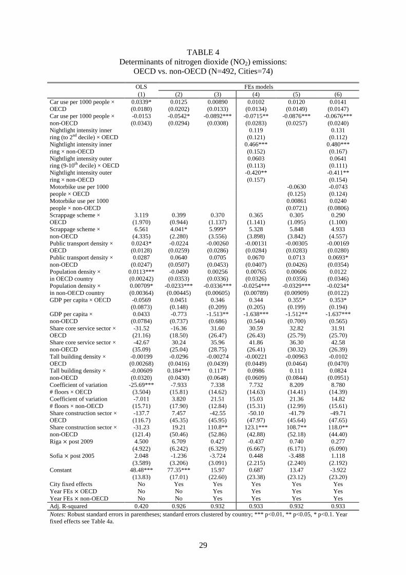
TABLE 4 Determinants of nitrogen dioxide (NO2) emissions:

OECD vs. non-OECD (N=492, Cities=74) OLS FEs models (1) (2) (3) (4) (5) (6) Car use per 1000 people × OECD

0.0339* 0.0125 0.00890 0.0102 0.0120 0.0141 (0.0180) (0.0202) (0.0133) (0.0134) (0.0149) (0.0147)

Car use per 1000 people × non-OECD

-0.0153 -0.0542* -0.0892*** -0.0715** -0.0876*** -0.0676*** (0.0343) (0.0294) (0.0308) (0.0283) (0.0257) (0.0240)

Nightlight intensity inner ring (to 2nd decile) × OECD

0.119 0.131 (0.121) (0.112)

Nightlight intensity inner ring × non-OECD

0.466*** 0.480*** (0.152) (0.167)

Nightlight intensity outer ring (9-10th decile) × OECD

0.0603 0.0641 (0.113) (0.111)

Nightlight intensity outer ring × non-OECD

-0.420** -0.411** (0.157) (0.154)

Motorbike use per 1000 people × OECD

-0.0630 -0.0743 (0.125) (0.124)

Motorbike use per 1000 people × non-OECD

0.00861 0.0240 (0.0721) (0.0806)

Scrappage scheme × 3.119 0.399 0.370 0.365 0.305 0.290 OECD (1.970) (0.944) (1.137) (1.141) (1.095) (1.100) Scrappage scheme × 6.561 4.041* 5.999* 5.328 5.848 4.933 non-OECD (4.335) (2.280) (3.556) (3.898) (3.842) (4.557) Public transport density × OECD

0.0243* -0.0224 -0.00260 -0.00131 -0.00305 -0.00169 (0.0128) (0.0259) (0.0286) (0.0284) (0.0283) (0.0280)

Public transport density × non-OECD

0.0287 0.0640 0.0705 0.0670 0.0713 0.0693* (0.0247) (0.0507) (0.0453) (0.0407) (0.0426) (0.0354)

Population density × in OECD country

0.0113*** -0.0490 0.00256 0.00765 0.00606 0.0122 (0.00242) (0.0353) (0.0336) (0.0326) (0.0356) (0.0346)

Population density × in non-OECD country

0.00709* -0.0233*** -0.0336*** -0.0254*** -0.0329*** -0.0234* (0.00364) (0.00445) (0.00605) (0.00789) (0.00909) (0.0122)

GDP per capita × OECD -0.0569 0.0451 0.346 0.344 0.355* 0.353* (0.0873) (0.148) (0.209) (0.205) (0.199) (0.194)

GDP per capita × non-OECD

0.0433 -0.773 -1.513** -1.638*** -1.512** -1.637*** (0.0784) (0.737) (0.686) (0.544) (0.700) (0.565)

Share core service sector × -31.52 -16.36 31.60 30.59 32.82 31.91 OECD (21.16) (18.50) (26.47) (26.43) (25.79) (25.70) Share core service sector × -42.67 30.24 35.96 41.86 36.30 42.58 non-OECD (35.09) (25.04) (28.75) (26.41) (30.32) (26.39) Tall building density × -0.00199 -0.0296 -0.00274 -0.00221 -0.00963 -0.0102 OECD (0.00268) (0.0416) (0.0439) (0.0449) (0.0464) (0.0470) Tall building density × -0.00609 0.184*** 0.117* 0.0986 0.111 0.0824 non-OECD (0.0320) (0.0430) (0.0648) (0.0609) (0.0844) (0.0951) Coefficient of variation # floors × OECD

-25.69*** -7.933 7.338 7.732 8.209 8.780 (3.504) (15.81) (14.62) (14.63) (14.41) (14.39)

Coefficient of variation # floors × non-OECD

-7.011 3.820 21.51 15.03 21.36 14.82 (15.71) (17.90) (12.84) (15.31) (12.99) (15.61)

Share construction sector × -137.7 7.457 -42.55 -50.10 -41.79 -49.71 OECD (116.7) (45.35) (45.95) (47.97) (45.64) (47.65) Share construction sector × -31.23 19.21 110.8** 123.1*** 108.7** 118.0** non-OECD (121.4) (50.46) (52.86) (42.88) (52.18) (44.40) Riga × post 2009 4.500 6.709 0.427 -0.437 0.740 0.277 (4.922) (6.242) (6.329) (6.667) (6.171) (6.090) Sofia × post 2005 2.048 -1.236 -3.724 0.448 -3.488 1.118 (3.589) (3.206) (3.091) (2.215) (2.240) (2.192) Constant 48.48*** 77.35*** 15.97 0.687 13.47 -3.922 (13.83) (17.01) (22.60) (23.38) (23.12) (23.20) City fixed effects No Yes Yes Yes Yes Yes Year FEs × OECD No No Yes Yes Yes Yes Year FEs × non-OECD No No Yes Yes Yes Yes Adj. R-squared 0.420 0.926 0.932 0.933 0.932 0.933 Notes: Robust standard errors in parentheses; standard errors clustered by country; *** p<0.01, ** p<0.05, * p<0.1. Year fixed effects see Table 4a.

29

TABLE 4a Year fixed effects corresponding to Table 4

OLS FEs models (1) (2) (3) (4) (5) (6) Year = 2006 × OECD 0.0762 -0.0848 0.130 -0.0350 (omitted year =2005) (0.841) (0.916) (0.882) (0.950) Year = 2007 × OECD -2.249** -2.681** -2.097* -2.537* (0.997) (1.271) (1.172) (1.408) Year = 2008 × OECD -3.414** -3.862** -3.193* -3.639* (1.431) (1.696) (1.648) (1.880) Year = 2009 × OECD -3.601** -4.070** -3.334* -3.795** (1.482) (1.664) (1.657) (1.835) Year = 2010 × OECD -4.122** -5.508** -3.853* -5.303* (1.736) (2.539) (1.961) (2.708) Year = 2011 × OECD -5.137** -5.891** -4.882** -5.654** (2.041) (2.375) (2.272) (2.576) Year = 2006 × non-OECD 2.266** 1.810* 2.239* 1.715 (omitted year =2005) (1.080) (1.054) (1.122) (1.229) Year = 2007 × non-OECD 3.069** 2.452** 3.008** 2.246 (1.155) (1.032) (1.347) (1.392) Year = 2008 × non-OECD 4.040 2.961 3.933 2.616 (2.577) (2.096) (3.014) (2.784) Year = 2009 × non-OECD 4.705 3.130 4.572 2.758 (2.816) (2.625) (3.284) (3.183) Year = 2010 × non-OECD 6.049** 5.391* 5.887* 4.807 (2.987) (2.832) (3.426) (3.635) Year = 2011 × non-OECD 10.58** 9.201** 10.38** 8.554 (4.046) (3.887) (4.934) (5.214) Notes: Robust standard errors in parentheses; standard errors clustered by country; *** p<0.01, ** p<0.05, * p<0.1.

30

TABLE 5 Determinants of sulphur dioxide (SO2) emissions:

Base specifications (N=450, Cities=70)

OLS FEs models (1) (2) (3)

Car use per 1000 people -0.0436*** -0.0358*** -0.0326*** (0.0151) (0.0122) (0.00982) Dummy old car scrappage scheme in place

-0.104 -0.167 0.216 (1.238) (0.378) (0.391)

Passengers in public transport per 1000 people

-0.000853 -0.0316* -0.0331** (0.00889) (0.0175) (0.0155)

Population density -0.00252 -0.0466*** -0.0439*** (0.00175) (0.00315) (0.00367) GDP per capita -0.107* -0.0941 -0.0323 (0.0554) (0.141) (0.211) Share of GDP from core service -49.15** -32.12 -9.233 industries (21.89) (21.26) (24.67) Tall building density (> 5 stories) 0.00342 0.0201 0.0493* (0.00260) (0.0285) (0.0269) Coefficient of variation # of floors 12.36*** 0.759 6.619 (4.151) (7.231) (8.203) Share of GDP from construction sector

-99.44 -4.461 -14.32 (65.40) (14.93) (12.52)

Year = 2006 -0.568 (omitted year =2005) (0.776) Year = 2007 -0.796 (1.094) Year = 2008 -1.448 (1.175) Year = 2009 -1.897* (1.032) Year = 2010 -2.504** (1.056) Year = 2011 -2.078** (0.906) Riga × post 2009 -18.60*** -10.18*** -8.548*** (5.852) (2.570) (2.233) Sofia × post 2005 0.0717 -7.070*** -6.689*** (2.174) (0.984) (0.758) Constant 58.03*** 90.91*** 70.38*** (19.96) (12.33) (16.30) City fixed effects No Yes Yes Adj. R-squared 0.587 0.953 0.954 Notes: Robust standard errors in parentheses; standard errors clustered by country; *** p<0.01, ** p<0.05, * p<0.1.

31

TABLE 6 Determinants of sulphur dioxide (SO2) emissions:

OECD vs. non-OECD (N=450, Cities=70)

OLS FEs models (1) (2) (3) (4) (5) (6) Car use per 1000 people × OECD

-0.00102 -0.0111* -0.0125** -0.0120** -0.0102* -0.00932 (0.00680) (0.00613) (0.00570) (0.00543) (0.00602) (0.00570)

Car use per 1000 people × non-OECD

-0.109*** -0.0748*** -0.0512 -0.0519 -0.0507 -0.0500 (0.0249) (0.0270) (0.0352) (0.0381) (0.0370) (0.0392)

Nightlight intensity inner ring (to 2nd decile) × OECD

0.0473 0.0551 (0.0562) (0.0537)

Nightlight intensity inner ring × non-OECD

0.154 0.160 (0.281) (0.283)

Nightlight intensity outer ring (9-10th decile) × OECD

0.0137 0.0151 (0.0397) (0.0391)

Nightlight intensity outer ring × non-OECD

0.0200 0.0257 (0.270) (0.250)

Motorbike use per 1000 people × OECD

-0.0432 -0.0468 (0.0325) (0.0332)

Motorbike use per 1000 people × non-OECD

0.00266 0.0122 (0.0720) (0.0663)

Scrappage scheme × -0.0717 0.000362 -0.0743 -0.0525 -0.115 -0.0932 OECD (0.703) (0.280) (0.482) (0.475) (0.476) (0.467) Scrappage scheme × -3.568 2.018 1.968 2.063 1.923 1.872 non-OECD (4.457) (1.617) (1.180) (1.262) (1.702) (1.714) Public transport density × OECD

-0.00799 -0.0181 -0.00618 -0.00521 -0.00637 -0.00524 (0.00664) (0.0121) (0.0113) (0.0117) (0.0114) (0.0119)

Public transport density × non-OECD

0.0594** -0.0533** -0.0677*** -0.0682*** -0.0674*** -0.0669*** (0.0238) (0.0241) (0.0190) (0.0192) (0.0221) (0.0215)

Population density × in OECD country

-0.00125 -0.0139 0.0110 0.0123 0.0133 0.0151 (0.00131) (0.0100) (0.0103) (0.0109) (0.0106) (0.0113)

Population density × in non-OECD country

-0.00656*** -0.0410*** -0.0335*** -0.0331*** -0.0332*** -0.0323*** (0.00150) (0.00600) (0.00871) (0.00860) (0.00862) (0.00878)

GDP per capita × OECD -0.0726* 0.0163 0.197** 0.195** 0.202** 0.200** (0.0381) (0.0865) (0.0881) (0.0873) (0.0851) (0.0842)

GDP per capita × non-OECD

-0.149** -0.448 -0.219 -0.252 -0.218 -0.251 (0.0684) (0.529) (0.517) (0.520) (0.523) (0.517)

Share core service sector × -55.37*** -20.16* 1.636 1.639 2.646 2.712 OECD (16.68) (10.96) (13.65) (14.19) (14.08) (14.67) Share core service sector × -44.75 -40.46 -27.14 -28.54 -27.00 -28.01 non-OECD (35.42) (46.56) (50.30) (48.89) (49.81) (48.92) Tall building density × 0.0106*** -0.0555 -0.0391 -0.0384 -0.0452 -0.0448 OECD (0.00188) (0.0531) (0.0482) (0.0486) (0.0504) (0.0509) Tall building density × -0.00374 0.0848*** 0.116*** 0.121*** 0.115** 0.116** non-OECD (0.0130) (0.0215) (0.0357) (0.0407) (0.0558) (0.0544) Coefficient of variation # floors × OECD

-2.049 -10.02** -1.510 -1.400 -1.019 -0.859 (3.090) (3.924) (4.616) (4.563) (4.448) (4.385)

Coefficient of variation # floors × non-OECD

38.34*** 18.14* 12.76 13.63 12.75 13.71 (9.707) (10.78) (16.11) (17.37) (16.19) (17.29)

Share construction sector × -168.8** -1.574 -28.31 -29.81 -27.67 -29.30 OECD (67.89) (17.87) (19.05) (18.14) (19.06) (17.98) Share construction sector × -26.23 7.519 -23.84 -18.37 -24.49 -21.07 non-OECD (99.60) (33.02) (51.79) (58.25) (50.74) (55.80) Riga × post 2009 -9.625** -16.67*** -13.05** -14.15** -12.95** -13.77* (3.698) (4.568) (5.254) (6.657) (6.341) (7.339) Sofia × post 2005 -3.926 -7.540** -4.026 -3.429 -3.963 -3.144 (2.590) (3.225) (3.288) (3.371) (2.798) (3.025) Constant 50.61*** 64.10*** 28.11** 22.96 26.58** 20.22 (15.71) (8.975) (10.82) (14.09) (11.82) (15.21) City fixed effects No Yes Yes Yes Yes Yes Year FEs × OECD No No Yes Yes Yes Yes Year FEs × non-OECD No No Yes Yes Yes Yes Adj. R-squared 0.767 0.958 0.960 0.959 0.959 0.959 Notes: Robust standard errors in parentheses; standard errors clustered by country; *** p<0.01, ** p<0.05, * p<0.1. Year fixed effects see Table 4a.

32

TABLE 6a Year fixed effects corresponding to Table 6

OLS FEs models (1) (2) (3) (4) (5) (6) Year = 2006 × OECD -0.353 -0.410 -0.309 -0.370 (omitted year =2005) (0.276) (0.288) (0.284) (0.290) Year = 2007 × OECD -1.206** -1.349** -1.087** -1.242** (0.462) (0.519) (0.516) (0.554) Year = 2008 × OECD -1.826*** -1.974*** -1.658*** -1.814*** (0.499) (0.587) (0.569) (0.633) Year = 2009 × OECD -1.638** -1.816** -1.443* -1.631* (0.716) (0.836) (0.753) (0.856) Year = 2010 × OECD -2.380** -2.826** -2.173** -2.664** (0.884) (1.152) (0.951) (1.169) Year = 2011 × OECD -2.738*** -2.979*** -2.547*** -2.807*** (0.814) (0.933) (0.895) (0.984) Year = 2006 × non-OECD -3.395 -3.615 -3.403 -3.660 (omitted year =2005) (2.272) (2.567) (2.226) (2.538) Year = 2007 × non-OECD -2.621 -3.045 -2.642 -3.160 (2.795) (3.321) (2.843) (3.359) Year = 2008 × non-OECD -3.477 -4.056 -3.511 -4.237 (2.885) (3.695) (2.900) (3.701) Year = 2009 × non-OECD -4.944* -5.234* -4.987** -5.432* (2.457) (2.894) (2.238) (2.814) Year = 2010 × non-OECD -6.492** -7.677* -6.546** -7.994** (2.758) (3.807) (2.734) (3.253) Year = 2011 × non-OECD -5.687* -6.481* -5.754 -6.823** (3.367) (3.498) (3.522) (3.225) Notes: Robust standard errors in parentheses; standard errors clustered by country; *** p<0.01, ** p<0.05, * p<0.1.

33

TABLE 7 Determinants of particulate matter (PM10) emissions:

Base specifications (N=425, Cities=67)

OLS FEs models (1) (2) (3)

Car use per 1000 people -0.0949*** -0.0243 -0.0201 (0.0325) (0.0360) (0.0310) Dummy old car scrappage scheme in place

2.035 -0.694 0.652 (3.311) (1.249) (1.689)

Passengers in public transport per 1000 people

0.000258 0.0160 0.0182 (0.0162) (0.0446) (0.0380)

Population density -0.000263 -0.0309*** -0.0242*** (0.00390) (0.0101) (0.00722) GDP per capita 0.0411 0.113 0.346 (0.151) (0.288) (0.305) Share of GDP from core service -87.47*** -73.78*** 2.187 industries (27.85) (22.07) (27.73) Tall building density (> 5 stories) -0.0616*** -0.0234 0.0640* (0.0216) (0.0464) (0.0357) Coefficient of variation # of floors 16.81 -19.07 -2.178 (10.23) (27.10) (24.44) Share of GDP from construction sector

73.50 -41.45 -49.50 (115.2) (60.49) (63.75)

Year = 2006 0.690 (omitted year =2005) (0.686) Year = 2007 -1.666 (1.164) Year = 2008 -4.460*** (1.176) Year = 2009 -5.442*** (1.664) Year = 2010 -6.161*** (1.715) Year = 2011 -5.054*** (1.449) Riga × post 2009 -20.36*** -14.59** -9.192* (6.632) (6.158) (5.439) Sofia × post 2005 15.94*** -3.043 -3.560 (4.815) (2.472) (2.133) Constant 109.2*** 116.3*** 52.12** (18.55) (17.67) (20.22) City fixed effects No Yes Yes Adj. R-squared 0.566 0.957 0.961 Notes: Robust standard errors in parentheses; standard errors clustered by country; *** p<0.01, ** p<0.05, * p<0.1.

34

TABLE 8 Determinants of particulate matter (PM10) emissions:

OECD vs. non-OECD (N=425, Cities=67) OLS FEs models (1) (2) (3) (4) (5) (6) Car use per 1000 people × OECD

-0.0251 0.0292* 0.0218 0.0257* 0.0168 0.0207 (0.0296) (0.0157) (0.0131) (0.0141) (0.0187) (0.0200)

Car use per 1000 people × non-OECD

-0.219*** -0.147* -0.0138 -0.0200 0.0154 0.00630 (0.0553) (0.0810) (0.0450) (0.0479) (0.0419) (0.0460)

Nightlight intensity inner ring (to 2nd decile) × OECD

0.202** 0.190** (0.0851) (0.0937)

Nightlight intensity inner ring × non-OECD

-0.140 -0.0586 (0.234) (0.212)

Nightlight intensity outer ring (9-10th decile) × OECD

-0.0934 -0.0978 (0.106) (0.101)

Nightlight intensity outer ring × non-OECD

0.118 0.202 (0.261) (0.251)

Motorbike use per 1000 people × OECD

0.0882 0.0840 (0.123) (0.124)

Motorbike use per 1000 people × non-OECD

0.162** 0.168** (0.0791) (0.0833)

Scrappage scheme × -0.228 0.0646 0.206 0.386 0.290 0.461 OECD (1.770) (0.780) (1.061) (1.036) (1.146) (1.119) Scrappage scheme × 24.15* -3.849 -6.997 -6.815 -9.736* -9.437* non-OECD (13.39) (7.877) (5.138) (5.138) (5.315) (5.328) Public transport density × OECD

0.00362 0.0137 0.0305 0.0355 0.0320 0.0367 (0.0129) (0.0209) (0.0225) (0.0238) (0.0226) (0.0237)

Public transport density × non-OECD

0.0128 -0.00637 -0.0546 -0.0542 -0.0388 -0.0387 (0.0437) (0.0642) (0.0629) (0.0632) (0.0582) (0.0580)

Population density × in OECD country

0.00336 -0.0507** -0.0208 -0.0139 -0.0262 -0.0193 (0.00372) (0.0246) (0.0299) (0.0297) (0.0314) (0.0315)

Population density × in non-OECD country

-0.0131*** -0.0291* 0.00628 0.00406 0.0191 0.0166 (0.00461) (0.0151) (0.0172) (0.0181) (0.0177) (0.0188)

GDP per capita × OECD -0.187** -0.131 0.227 0.199 0.220 0.192 (0.0731) (0.209) (0.189) (0.200) (0.196) (0.203)

GDP per capita × non-OECD

0.835*** 1.504 2.662** 2.703** 2.703** 2.739** (0.0643) (1.207) (1.007) (1.010) (1.021) (1.030)

Share core service sector × -57.68* -67.29*** -25.78 -29.66 -27.01 -30.76 OECD (30.32) (18.07) (19.26) (18.62) (19.97) (19.18) Share core service sector × 23.06 -43.09 44.41 42.90 56.27 54.32 non-OECD (53.05) (37.91) (70.10) (68.47) (71.73) (70.10) Tall building density × -0.0443** -0.0152 0.0149 0.0282 0.0304 0.0429 OECD (0.0196) (0.0594) (0.0670) (0.0743) (0.0516) (0.0576) Tall building density × 0.0214 0.0302 0.143** 0.137** 0.0867 0.0821 non-OECD (0.0205) (0.0639) (0.0652) (0.0637) (0.0531) (0.0522) Coefficient of variation # floors × OECD

-3.030 -23.33*** -8.814 -10.17 -9.884 -11.24 (6.620) (5.814) (6.458) (6.269) (7.157) (6.833)

Coefficient of variation # floors × non-OECD

11.72 -11.31 -42.15 -40.15 -42.49 -38.81 (31.01) (53.57) (63.55) (63.70) (62.50) (62.64)

Share construction sector × -237.8* 3.567 -14.57 -7.626 -16.16 -8.764 OECD (128.4) (43.73) (55.75) (53.30) (57.22) (55.24) Share construction sector × 108.6 -94.76 -258.0*** -260.2*** -296.7*** -295.9*** non-OECD (166.0) (93.09) (82.64) (84.78) (83.86) (85.53) Riga × post 2009 -26.68*** -27.91** -5.682 -5.553 0.583 -0.0924 (7.433) (11.16) (7.697) (7.456) (8.666) (8.663) Sofia × post 2005 14.86* -14.61* -4.216 -5.509 -0.295 -1.492 (7.687) (8.128) (5.194) (5.967) (4.350) (5.317) Constant 93.63*** 113.0*** 39.04* 31.93 31.17 23.23 (18.36) (17.03) (20.08) (19.63) (21.99) (21.73) City fixed effects No Yes Yes Yes Yes Yes Year FEs × OECD No No Yes Yes Yes Yes Year FEs × non-OECD No No Yes Yes Yes Yes Adj. R-squared 0.734 0.960 0.967 0.967 0.968 0.968 Notes: Robust standard errors in parentheses; standard errors clustered by country; *** p<0.01, ** p<0.05, * p<0.1. Year fixed effects see Table 4a.

35

TABLE 8a Year fixed effects corresponding to Table 8

OLS FEs models (1) (2) (3) (4) (5) (6) Year = 2006 × OECD 0.151 0.112 0.0473 0.0286 (omitted year =2005) (0.610) (0.605) (0.636) (0.641) Year = 2007 × OECD -2.263** -2.377** -2.540*** -2.604*** (0.993) (0.962) (0.917) (0.951) Year = 2008 × OECD -3.964*** -4.140*** -4.364*** -4.484*** (1.081) (1.043) (0.946) (0.973) Year = 2009 × OECD -2.980** -3.156** -3.432** -3.544*** (1.474) (1.270) (1.335) (1.178) Year = 2010 × OECD -3.721** -3.856** -4.174*** -4.158*** (1.580) (1.453) (1.344) (1.442) Year = 2011 × OECD -3.340* -3.570** -3.767** -3.913*** (1.824) (1.674) (1.481) (1.415) Year = 2006 × non-OECD -2.105 -1.879 -2.710 -2.686 (omitted year =2005) (2.150) (2.203) (2.280) (2.341) Year = 2007 × non-OECD -6.142 -5.831 -7.595* -7.706* (3.742) (3.792) (3.830) (3.903) Year = 2008 × non-OECD -12.75* -12.28* -15.07** -15.10** (6.788) (6.742) (6.983) (7.008) Year = 2009 × non-OECD -19.12** -18.47** -22.05** -21.61** (8.340) (8.242) (8.521) (8.540) Year = 2010 × non-OECD -22.71** -22.27** -26.31*** -27.13** (8.838) (9.527) (9.347) (10.11) Year = 2011 × non-OECD -25.27** -24.68** -29.77*** -29.94*** (9.928) (9.989) (10.75) (10.87) Notes: Robust standard errors in parentheses; standard errors clustered by country; *** p<0.01, ** p<0.05, * p<0.1.

36

FIGURES

FIGURE 1 Mean annual concentrations of NO2, SO2, and PM10 (2005-2011; μg per m3)

(Samples only include cities that have observations for all 7 years)

3638

4042

44

2005 2006 2007 2008 2009 2010 2011year

Full sample OECD onlynon-OECD only

Mean annual concentration of NO2Panel A

010

2030

40

2005 2006 2007 2008 2009 2010 2011year

Full sample OECD onlynon-OECD only

Mean annual concentration of SO2Panel B

3040

5060

70

2005 2006 2007 2008 2009 2010 2011year

Full sample OECD onlynon-OECD only

Mean annual concentration of PM10Panel C

37

FIGURE 2 Mean annual concentrations of NO2, SO2, and PM10 by city

(Selected cities; 2005-2011; measured in μg per m3)

Panel A: NO2

Panel B: SO2

Panel C: PM10

2040

6080

2040

6080

2005 20112005 20112005 2011

Athens Beijing Bogota

Dublin London OsakaNO2

yearGraphs by city

020

4060

020

4060

2005 20112005 20112005 2011

Athens Beijing Bogota

Dublin London OsakaSO2

yearGraphs by city

050

100150

050

100150

2005 20112005 20112005 2011

Athens Beijing Bogota

Dublin London OsakaPM10

yearGraphs by city

38

APPENDICES

Appendix A: Appendix Tables

TABLE A1 Cities included in base specifications (Tables 3 and 4) (N=75)

City Country OECD City Country OECD Abu Dhabi United Arab Emirates No Melbourne Australia Yes Amsterdam The Netherlands Yes Mexico City Mexico No Antwerp Belgium Yes Miami United States Yes Athens Greece Yes Milan Italy Yes Auckland New Zealand Yes Minsk Belarus No Bangkok Thailand No Montreal Canada Yes Barcelona Spain Yes Munich Germany Yes Beijing China No Nagoya Japan Yes Belgrade Serbia No New York United States Yes Berlin Germany Yes Osaka Japan Yes Birmingham United Kingdom Yes Oslo Norway Yes Bogota Colombia No Paris France Yes Bratislava Slovakia Yes Phoenix United States Yes Brussels Belgium Yes Prague Czech Republic Yes Bucharest Romania No Riga Latvia No Budapest Hungary No Rome Italy Yes Buenos Aires Argentina No Rotterdam The Netherlands Yes Chicago United States Yes San Francisco United States Yes Copenhagen Denmark Yes Santiago Chile Yes Dublin Ireland Yes Sarajevo Bosnia & Herzegovina No Frankfurt Germany Yes Shanghai China No Geneva Switzerland Yes Sofia Bulgaria No Glasgow United Kingdom Yes Stockholm Sweden Yes Gothenburg Sweden Yes Sydney Australia Yes Guangzhou China No São Paulo Brazil No Hamburg Germany Yes Taipei Taiwan No Helsinki Finland Yes Tallinn Estonia No Houston United States Yes Tianjin China No Istanbul Turkey Yes Tokyo Japan Yes Leeds United Kingdom Yes Toronto Canada Yes Lisbon Portugal Yes Vancouver Canada Yes Ljubljana Slovenia Yes Vienna Austria Yes London United Kingdom Yes Vilnius Lithuania No Los Angeles United States Yes Warsaw Poland Yes Lyon France Yes Wuhan China No Madrid Spain Yes Zagreb Croatia No Manchester United Kingdom Yes Zurich Switzerland Yes Marseille France Yes Notes: For NO2 no information is available for Istanbul. For SO2, no information is available for: Buenos Aires, Geneva, Miami, Oslo and San Francisco. For PM10, no information is available for Chicago, Istanbul, Los Angeles, Miami, New York, Phoenix, San Francisco and Toronto.

39

TABLE A2 City center coordinates and sources (N=75)

City Latitude Longitude City Latitude Longitude Abu Dhabi 24.466884 54.366267 Melbourne -37.814460 144.963230 Amsterdam 52.370314 4.894840 Mexico City 19.431837 -99.133302 Antwerp 51.219546 4.402578 Miami* 25.788043 -80.224729 Athens 37.984072 23.729241 Milan 45.465455 9.185897 Auckland -36.848738 174.762473 Minsk 53.899670 27.567165 Bangkok 13.727435 100.523762 Montreal 45.509161 -73.554155 Barcelona 41.385131 2.173401 Munich 48.135095 11.581833 Beijing 39.903601 116.407072 Nagoya 35.181240 136.905420 Belgrade 44.821334 20.461864 New York* 40.715387 -74.005895 Berlin* 52.522488 13.405323 Osaka 34.693645 135.502360 Birmingham 52.486010 -1.890582 Oslo 59.913998 10.751986 Bogota 4.597317 -74.075381 Paris 48.856544 2.352167 Bratislava 48.145832 17.107076 Phoenix 33.449149 -112.073553 Brussels 50.850298 4.351646 Prague 50.075206 14.437643 Bucharest 44.432249 26.103478 Riga 56.949433 24.104872 Budapest 47.497801 19.040009 Rome* 41.893844 12.482944 Buenos Aires -34.603879 -58.381757 Rotterdam 51.924108 4.481566 Chicago 41.877844 -87.630017 San Francisco 37.774527 -122.419061 Copenhagen 55.676011 12.568134 Santiago -33.469833 -70.641894 Dublin 53.349638 -6.260621 Sarajevo -23.550451 -46.633236 Frankfurt 50.110755 8.682226 Shanghai 43.856272 18.413068 Geneva 46.198467 6.142100 Sofia 41.997177 21.428152 Glasgow 55.864227 -4.251942 Stockholm 42.697198 23.32017 Gothenburg 57.708742 11.974020 Sydney 59.329032 18.064622 Guangzhou 23.130649 113.258057 São Paulo -33.867474 151.206892 Hamburg 53.551332 9.993739 Taipei* 25.04625 121.51753 Helsinki 60.173330 24.941036 Tallinn 59.437094 24.753691 Houston 29.759970 -95.369362 Tianjin 39.083470 117.200775 Istanbul 41.005322 28.975787 Tokyo 35.688960 139.690475 Leeds 53.801263 -1.548521 Toronto 43.652929 -79.383278 Lisbon 38.722469 -9.139604 Vancouver 49.261011 -123.114119 Ljubljana 46.056350 14.507895 Vienna 48.208217 16.373537 London 51.508505 -0.125637 Vilnius 54.686854 25.279349 Los Angeles 34.053501 -118.243504 Warsaw 52.229626 21.012185 Lyon 45.764123 4.835636 Wuhan 30.592501 114.305363 Madrid 40.416397 -3.703913 Zagreb 45.813641 15.979094 Manchester 53.479346 -2.248483 Zurich 47.368562 8.539204 Marseille 43.296385 5.369433 Sources: Coordinates are ‘central points’ of city according to Google Map (last accessed 3/5/2014). *Google Map coordinates were deemed unrealistic for the following cities (Google Map coordinates in brackets): Berlin (52.493748; 13.455324), Miami (25.789125; -80.204988), New York (40.705501; -73.978089), Rome (41.872246; 12.480380) and Taipei (25.093179; 121.559098). For these cities we identified ‘quasi-official’ centers using Google search and the coordinates of these centers are given above. The distances between ‘Google Map centers’ and ‘Google search centers’ are: 4.7km (Berlin), 2.0km (Miami), 2.6km (New York), 6.7km (Taipei). Results are virtually unchanged if Google Map coordinates are used for all 75 cities.

40

TABLE A3 Robustness checks: Add relative fuel price and remove outliers

(Based on final specifications) Type of check: Add relative price diesel/petrol Remove top and bottom three outliers

N: 455 413 397 450 408 383 (1)

NO2 (2) SO2

(3) PM10

(4) NO2

(5) SO2

(6) PM10

Relative price of diesel to petrol × OECD

-1.222 -6.354 0.738 (8.299) (5.800) (10.51)

Relative price of diesel to petrol × non-OECD

-28.21* -3.956 34.51 (15.88) (8.993) (25.19)

Car use per 1000 people × OECD

0.0176 -0.00872 0.0199 -0.00187 -0.0104* 0.0347** (0.0151) (0.00529) (0.0196) (0.0118) (0.00581) (0.0151)

Car use per 1000 people × non-OECD

-0.0697** -0.0420 0.0595 -0.0715*** -0.0787** 0.0625 (0.0269) (0.0404) (0.0515) (0.0232) (0.0308) (0.0472)

Nightlight intensity inner ring (to 2nd decile) × OECD

0.108 0.0205 0.164* 0.129 0.104** 0.203** (0.118) (0.0497) (0.0972) (0.104) (0.0456) (0.0959)

Nightlight intensity inner ring × non-OECD

0.334** 0.159 0.0645 0.382* 0.262 -0.0101 (0.147) (0.285) (0.221) (0.212) (0.340) (0.235)

Nightlight intensity outer ring (9-10th decile) × OECD

0.0566 0.0444 -0.105 0.0502 0.0116 -0.130 (0.123) (0.0464) (0.103) (0.0907) (0.0429) (0.0868)

Nightlight intensity outer ring × non-OECD

-0.430*** 0.0193 0.278 -0.274 0.236 -0.201 (0.145) (0.276) (0.259) (0.176) (0.245) (0.226)

Motorbike use per 1000 people × OECD

-0.0894 -0.0645* 0.0887 -0.0804 -0.0347 -0.0116 (0.131) (0.0339) (0.121) (0.123) (0.0312) (0.0814)

Motorbike use per 1000 people × non-OECD

0.0370 0.0308 0.230*** -0.162*** 0.0397 0.221** (0.0735) (0.0766) (0.0775) (0.0517) (0.0791) (0.108)

Scrappage scheme × 0.621 0.0184 0.551 0.268 -0.0267 -0.119 OECD (1.312) (0.424) (1.249) (1.033) (0.446) (0.935) Scrappage scheme × 4.809 1.415 -11.47** -1.114 0.606 4.199 non-OECD (4.532) (1.794) (4.788) (2.113) (2.271) (5.348) Public transport density × OECD

0.00117 -0.00853 0.0300 -0.0106 -0.00205 0.0384 (0.0289) (0.0116) (0.0245) (0.0234) (0.0137) (0.0236)

Public transport density × non-OECD

0.0865** -0.0612*** -0.0349 0.0259 -0.0567*** -0.0610 (0.0380) (0.0214) (0.0523) (0.0567) (0.0179) (0.0672)

Population density × in OECD country

0.0150 0.0140 -0.0197 0.0131 0.0207* -0.0103 (0.0384) (0.0111) (0.0328) (0.0332) (0.0106) (0.0295)

Population density × in non-OECD country

-0.0305** -0.0327*** 0.0207 -0.0244*** -0.0287 0.0402* (0.0127) (0.00918) (0.0190) (0.00725) (0.0185) (0.0228)

GDP per capita × OECD 0.314 0.193** 0.229 0.322* 0.205** 0.101 (0.216) (0.0835) (0.208) (0.188) (0.0855) (0.156)

GDP per capita × non-OECD

-1.697** -0.132 3.408*** -1.497** -0.274 2.216* (0.642) (0.521) (1.060) (0.596) (0.444) (1.273)

Share core service sector × 33.65 4.239 -32.56 5.613 8.151 -27.93 OECD (26.37) (14.30) (19.39) (21.87) (13.84) (18.94) Share core service sector × 52.30 -22.16 93.05 -10.66 23.34 -10.67 non-OECD (31.45) (48.18) (70.21) (33.27) (38.50) (90.10) Tall building density × -0.0138 -0.0759 0.0205 -0.0234 -0.0403 0.0739* OECD (0.0503) (0.0512) (0.0628) (0.0395) (0.0488) (0.0427) Tall building density × 0.215** 0.119** 0.0522 0.112* 0.107* 0.0744 non-OECD (0.102) (0.0552) (0.0559) (0.0640) (0.0536) (0.0568) Coefficient of variation # floors × OECD

5.067 -0.195 -8.485 13.96 0.982 -5.776 (14.29) (4.410) (6.219) (12.33) (3.426) (8.592)

Coefficient of variation # floors × non-OECD

26.11 13.14 -53.55 17.58 24.30 -22.24 (19.82) (17.81) (54.72) (16.04) (14.95) (78.33)

Share construction sector × -45.68 -24.80 -7.356 -30.51 -22.72 -23.30 OECD (49.70) (17.82) (58.23) (46.50) (17.75) (46.68) Share construction sector × 170.9*** -23.89 -380.4*** 208.8*** 14.73 -279.3*** non-OECD (47.08) (64.54) (108.4) (55.53) (82.17) (73.19) Other controls and fixed effects as in columns (6) of Tables 4, 6, and 8

Yes Yes Yes Yes Yes Yes

Adj. R-squared 0.346 0.625 0.495 0.307 0.556 0.446

Notes: Robust standard errors in parentheses; standard errors clustered by country; *** p<0.01, ** p<0.05, * p<0.1.

41

Appendix B: Appendix Figure

FIGURE A1 Time-series of explanatory variables: All cities, OECD only and non-OECD only

(Samples only include cities that have observations for all 7 years; Panel A excludes Riga and Sofia due to change in definition of explanatory variable)

100

200

300

400

500

2005 2006 2007 2008 2009 2010 2011year

Full sample OECD onlynon-OECD only

Car use per 1000 peoplePanel A

48

50

52

54

56

58

2005 2006 2007 2008 2009 2010 2011year

Full sample OECD onlynon-OECD only

Nightlight intensity inner ring (1st and 2nd decile)Panel B

15

20

25

30

35

2005 2006 2007 2008 2009 2010 2011year

Full sample OECD onlynon-OECD only

Nightlight intensity outer ring (9th and 10th decile)Panel C

30

40

50

60

70

80

2005 2006 2007 2008 2009 2010 2011year

Full sample OECD onlynon-OECD only

Motorbike use per 1000 peoplePanel D

42

FIGURE A1—Continued

0.2

.4.6

.8

2005 2006 2007 2008 2009 2010 2011year

Full sample OECD onlynon-OECD only

Scrappage scheme presentPanel E

180

200

220

240

260

2005 2006 2007 2008 2009 2010 2011year

Full sample OECD onlynon-OECD only

Passengers per 1000 peoplePanel F

600

800

100

01

20

01

40

0

2005 2006 2007 2008 2009 2010 2011year

Full sample OECD onlynon-OECD only

Population densityPanel G

10

20

30

40

50

2005 2006 2007 2008 2009 2010 2011year

Full sample OECD onlynon-OECD only

GDP per capitaPanel H

43

FIGURE A1—Continued

.35

.4.4

5.5

.55

2005 2006 2007 2008 2009 2010 2011year

Full sample OECD onlynon-OECD only

Share of GDP from core service industriesPanel I

20

40

60

80

100

2005 2006 2007 2008 2009 2010 2011year

Full sample OECD onlynon-OECD only

Tall building densityPanel J

.4.4

5.5

.55

.6

2005 2006 2007 2008 2009 2010 2011year

Full sample OECD onlynon-OECD only

Coefficient of variation # of floorsPanel K

.04

5.0

5.0

55

.06

.06

5

2005 2006 2007 2008 2009 2010 2011year

Full sample OECD onlynon-OECD only

Share of GDP from construction sectorPanel L

44

Appendix C: Technical Appendix (Detailed Description of Data and Sources)

1. Spatial distribution of pollution monitoring stations

Central points of metro areas

Given that there is no single way to define the ‘true’ central point of a city’s metro area, we did an initial online search (‘Google Search’) for commonly accepted city centers for a random sample of 15 cities. We then checked whether these centers are close to the center identified by Google Map. Since they were close in all cases, we used Google Map centers as a less arbitrary way of defining city centers, the coordinates of which can be seen in Appendix Table A2. Each city center was visually inspected. We identified five centers that appeared to be obviously ‘incorrect’. For example, Google Map gave the city center of New York City as being in the East River between Manhattan and Brooklyn. For those five cases, we used the centers suggested by Google Search instead. Note, however, that our results remain essentially unchanged if we use the Google Map coordinates for these five metro areas as the centers instead of the ones suggested by Google Search.

Numbers and locations of pollution monitoring stations

Identifying a reliable indicator for the number and location of monitoring stations was challenging due to, e.g. a lack of or contradictory information on locations, the existence of different types of stations, which measure different pollutants. Thus, numbers and locations of stations should be considered indicative, as they are based on those which primarily measured NO/NO2/NOX. These were benchmarked against stations which measured particulate matter. Moreover, numbers and locations of stations over the period between 2005 and 2011 were assumed constant due to data limitations. This assumption is supported by checking the data for cities, which had data on stations for more than a single year.

Three cities (Cairo, Montevideo and Skopje) were excluded from our original sample because over the study period (i) there was either evidence of a substantial number of new monitoring stations added to the existing stock of stations or (ii) there were critical technological or methodological changes in how pollution concentrations were measured, thus rendering year-to-year comparisons problematic. In all three cases, relevant year-to-year changes were implausibly high. For example, Cairo reported implausible falls in nitrogen dioxide concentrations between 2006 and 2007 (~50%) as well as between 2008 and 2009 (~30%). This was attributed to the addition of a number of new stations to the network thus resulting in increased accuracy in addition to efforts to reduce air pollution in the city.

Stations were identified by a variety of methods. In general, they were identified by internet searches with the city name as the key search term. For European, US and Canadian cities, station locations were provided in three separate databases: Airbase (EU), Environment Protection Agency (US) and Environment Canada (Canada). These databases provided coordinates in terms of latitude and longitude. For other cities, information was gathered from city authority websites, including government reports. The WHO Urban Outdoor Air Pollution database provided the number of particulate matter-monitoring stations in cities and

45

in some cases a link to the responsible pollution monitoring organisation. Where such links existed, database entries were created from the information gathered. Note that the quality of data from these sources varied. In particular, we are unable to distinguish between traffic stations and urban background stations for most of the cities in our sample. In a sample of German cities, Wolff (2014) shows that the percentage of observed particulate matter attributed to vehicle emissions tends to be higher for traffic stations in comparison to urban background stations. Yet for both types of stations, there is much variation in vehicles’ share of emissions.

City shape and size

Once the central points of metro areas and the numbers and locations of stations were identified and counted, assessing the distribution of stations also required estimates of the size of the metro area and a way of assessing how distance from the central point could be used as a measure of centrality, which depended on the shape of the city. Data for the population size, size and boundary of metro areas were sourced from Euromonitor. Based on the shape of the metro area visible from Google Map and/or Google Earth, cities were assigned to one of two shape ‘types’: circular or semi-circular. Both allowed for the estimation of a radius. This made it possible to estimate the proportion of stations that fell within deciles of the metro area, in concentric circles drawn around the central point. For cities, in which part of the full circle falls into the ocean, country boundaries are used to intersect the circle. This allowed for the identification of the proportion of the circle located in the ocean versus on land, which was in turn used to construct a circle big enough such that the metro area remains as reported by Euromonitor after the intersection of the circle with the boundary. We do, however, note the challenge of identifying metro area boundaries from Google Map alone for many cities.

2. Car scrappage schemes

Scrappage schemes were identified from three sources, which contained information about the timing and nature of schemes in each city:

• http://ec.europa.eu/enterprise/sectors/automotive/files/projects/report_scrapping_schemes_annex_en.pdf

• http://www.whatcar.com/car-news/european-schemes-work/1203776 • http://en.wikipedia.org/wiki/Scrappage_program

3. Spatial distribution and intensity of night lights

We utilize night-light data for our panel of cities in order to create an indicator of the spatial distribution of economic activity for each year between 2005 and 2011. For each city and year, we estimated the mean intensity of night lights within each and every decile of the metro area using the concentric circles created for the purpose of assessing the distribution of monitoring stations. This per-decile measure was estimated using data for total light intensity and the number of pixels located within each decile. Our focus on the changes in the intensity of night lights implies that changes in the size of the metro area over time are less relevant. Thus, fixing the boundaries of metro areas, we argue, is sufficient for obtaining an approximate indication of the scope of decentralization in each metro area. Our data report an

46

intensity of night lights ranging from 0 to 63, with 63 being the top-coded value. Top-coded data can be used to measure the spatial extent of night lights in any city. But since top coding is less of an issue in less-developed countries, measures of night light intensity could be considered a better measure of economic development in non-OECD cities than in OECD ones.

Note that in 2010, the satellite that was used to capture night lights changed. A fraction of the year-to-year changes in nightlight intensity between 2009 and 2010 can thus be attributed to the change in measurement-technology. Our year fixed effects should capture this ‘global shock’ to observed nightlight intensity.

4. Road grid system

From Google Maps, city centers in metro areas were judged on the extent to which they were laid out in a grid pattern. Three categories were created: no grid; partial or irregular grid; and, straight grid. For the purposes of our analysis we coded cities as being ‘straight grid’ only if they have a clear (unambiguous) straight grid (see also Footnote 11).

5. Distance to sea coast

Distance to coast was estimated by visual inspection of Google Maps and eyeballing the closest coast, noting the coordinates, and then calculating the distance from the estimated center. Sea coasts were always used rather than lakes. Distance was measured using the Great Circle Distance - the shortest path between two points on the surface of a sphere.

47