Embed Size (px)
Citation preview

University of MariborUniverza v Mariboru
Faculty of Civil EngineeringFakulteta za gradbeništvo
Mihael Peternelj
Rheology of Steel — Concrete Composite BridgesReologija jekleno — betonskih sovprežnih mostov
Bachelor’s degree
Diplomsko delo
Maribor, april 2009

I
Bachelor’s degree work from academic study program
Rheology of Steel — Concrete Composite BridgesReologija jekleno — betonskih sovprežnih mostov
Student: Mihael PeterneljStudy program: civil engineeringField: steel structuresMentor: red. prof. dr. Kravanja Stojan, univ. dipl. inž. grad.Comentor: Dorian Janjic, univ. dipl. inž. grad.Comentor: pred. Milan Kuhta, univ. dipl. inž. grad.
Maribor, april 2009

II

III
Words of gratitude
On this page i would like to expressmy gratitude to my mentor Dr. StojanKravanja, DI Dorian Janjic from BentleySystems Inc. (Graz) and Milan Kuhtauniv. dipl. inž. grad. on help and guidancetrough the writing of this work.
Special thanks go to my mother DušankaPeternelj, who solely enabled and sup-ported me in the years of studying andKatja Rade who helped writing.
IV
Reologija jekleno — betonskih sovprežnih mostov
Ključne besede: reologija, sovprežni mostovi, jeklo, beton, lezenje, krčenje, relak-sacija, CEB–FIP 1990, metoda končnih elementov, računska analiza konstrukcij.UDK: 666.97.035:624.21(043.2)
Povzetek
Osnovni namen diplomske naloge je predstaviti reološke vplive betona na sovprežnokonstrukcijo (kot njen sestavni material). V nadaljevanju bomo predstavili numeričnepostopke za izračun teh vplivov, ter rešili dva primera. Prvi poenostavljen primer,ki detajlno opisuje postopek in drugi (bolj zahteven) primer s pomočjo programskegapaketa RM Bridge, ki velja za enega najboljših programskih paketov za računsko analizomostov.
Diplomsko delo je sestavljeno iz dveh delov: teoretičnega in računskega dela. V prvemdelu je predstavljena teorija, pristop in formule, ki omogočajo natančno določanje re-oloških vplivov betona na sovprežno konstrukcijo kot njen sestavni element. Drugi delje v grobem sestavljen iz dveh računskih primerov. Prvi računski primer je enostavensovprežni nosilec podprt z dvema elastičnima podporama in služi zgolj v demonstativnenamene, ter detajlno prikazuje računski postopek analize konstrukcije. Primer je bilrešen ročno in rezultati računske analize konstrukcije primerjani z tistimi dobljenimis pomočjo programskega paketa RM Bridge. Drugi primer bolje ustreza realiteti. Vdrugem primeru je izračunan sovprežni most z tremi razponi dolžine 40 m – 60 m – 40m. Tak sovprežni most ustreza kakšnemu podobnemu mostu v praksi, zato se rezultatinjegove računske analize lahko primerjajo na realni osnovi.
Na podlagi rezultatov drugega primera lahko sklepamo, da je časovno odvisne materi-alne in reološke karakteristike betona, kot sestavnega materiala sovprežne konstrukcije,potrebno vedno upoštevati.

V
Rheology of Steel — Concrete Composite Bridges
Keywords: rheology, composite bridges, steel, concrete, creep, shrinkage, relaxation,CEB–FIP 1990, finite elements method, structural analysis.UDK: 666.97.035:624.21(043.2)
Summary
The main purpose of this diploma work is to discuss the time dependant effects ofconcrete as a component material of the composite construction and their influence. Inaddition numerical solutions for calculating creep and shrinkage effects will be presentedand two examples solved, one simpler with detailed description and one more difficultusing the leading software package RM Bridge for modelling bridges.
This work is divided into two parts: theoretical part and calculation part. In the firstpart theory, methodology and formulas that enable precise prediction of concrete timedependant parameters on the composite construction as a part of it. The second part ofthis work consists of two examples. First example is a very simplified composite beamheld up by two elastic supports. The main purpose of this much simplified example is fordemonstration purposes only. It was calculated manually with detailed description andthe results of structural analysis compared to those gained with help of software packageRM Bridge. Second example tends to be more realistic. In this case we have a threespan 40 m – 60 m – 40 m steel — concrete composite bridge. Such bridge correspondsto an average composite bridge in reality and therefore the results of structural analysiscan be evaluated on real ground basis.
Based on the results of the second example we can conclude that time dependent effectsof concrete as a material used in composite constructions always have to be considered.

VI
Povzetek poglavij v slovenskem jeziku
Predstavitev
Sovprežne konstrukcije predstavljajo bodočnost modernih konstrukcij. Njihova glavnaprednost je ravno v kombinaciji materialov, ki se po svojih lastnostih dopolnjujejo. Vtej diplomski naloge se bomo usredotočili predvsem na jekleno — betonske sovprežnekonstrukcije. Že prva posebnost kombinacije teh dveh materialov združenih v enemnosilnem elementu je naprimer podoben količnik toplotnega raztezanja. V primeru, daimamo normalno nosilno konstrukcijo, kot je recimo sovprežni most z betonsko ploščona vrhu jeklenih nosilcev, je ta kombinacija materiala ugodna še z drugega vidika.Beton je material, ki zelo dobro nosi tlačne napetosti a zelo slabo natezne. Ravnoobratno je pri jeklu. Ta material zelo dobro prenaša natezne napetosti in (zaradivitkosti tipičnih jeklenih prerezov) tlačne slabše. V takšni konstrukciji je stanje no-tranjih sil zgolj zaradi lastne teže zelo ugodno. Beton nosi tlačne napetosti na prerezu,jeklo pa natezne. V kolikor ta kombinacija materialov v tej obliki na začetku delujezelo dobro, se slika notranjih napetosti zaradi edinstvenih časovno odvisnih materialnihkarakteristik betona povsem spremeni.
Ravno to je cilj te diplomske naloge, predstaviti vpliv reoloških lastnosti betona nasovprežno konstrukcijo kot njenega sestavnega elementa, teorijo in postopek izračunaz upoštevanjem le–teh in primerjati rezultate notranjih sil v posameznem materialubrez in z upoštevanjem reologije betona. Pri tem bomo uporabili računski model poCEB-FIP 1990.
Časovno odvisne deformacije
Časovno odvisne deformacije so lahko odvisne ali neodvisne od napetosti. Časovnoodvisni deformaciji, ki nista odvisni od napetosti so predvsem krčenje (ang. shrinkage)ali nabrekanje (ang. swelling), medtem ko sta časovno odvisni deformaciji odvisni od

VII
napetosti v materialu lezenje (ang. creep) in relaksacija (ang. relaxation).
Krčenje oziroma nabrekanje je odvisno predvsem od okolišnih razmer, ki so v povezaviz izločanjem vode iz betona. Tako je krčenje definirano kot časovno odvisna spremembavolumna neobremenjenega vzorca.
Lezenje je definirano kot časovno odvisna sprememba deformacije zaradi stalne in kon-stantne napetosti v vzrocu primerjane z enakim a neobremenjenim vzorcem.
Zelo podoben pojav lezenju je relaksacija. Za razliko od lezenja, katerega definirasprememba deformacije, definira relaksacijo sprememba napetosti v vzorcu zaradi kon-stantne deformacije na vzorcu.
Poznamo veliko računskih modelov, ki opisujejo viskoelastično obnašanje betona. Mod-eli kot so Maxwell-ov, Kelvin-Voigt-ov ali Standard Linear Solid Model ima vsak svojoprednost pred drugim in delno natančno opisujejo deformacijsko obnašanje betona a sov praksi neuporabni saj ne upoštevajo zgodovine napetosti. Iz tega razloga je bil razvitmodel CEB–FIP 1990, ki z upoštevanjem zgodovine napetosti, ter okoljskih vplivovzelo natančno matematično opisuje razvoj deformacij v betonu.
Jekleno – betonski sovprežni mostovi
Sovprežne konstrukcije so zelo razširjen pojem. Obsegajo vse od enostavnih elementov,kot so temelji, nosilci in stebri, pa vse do loka mostu. Še večja je izbira materialov,ki obsega široko paleto kombinacij lesa in jekla, jekla in betona, lesa in betona, tudibetona in betona.
Izbor materialov uporabljenih v sovprežni konstrukciji je vitalnega pomena, saj le–tivitalno vplivajo na kasnejše obnašanje konstrukcije. Materiali so si lahko po lastnostihzelo različni, vendar je ravno izkoriščanje teh razlik na pravi način ključna prednostsovprežnih konstrukcij. Pri kombinaciji jekla in betona se izkorišča velika tlačna nosil-nost betona in velika natezna nosilnost jekla. Kombinacija v obratnem smislu ne bidelovala, saj bi se jekleni nosilec pod tlačno napetostjo zaradi svoje vitkosti uklonil,beton pa bi zaradi slabe natezne nosilnosti popokal.
Sovprežne konstrukcije iz ekonomskega vidika imajo ozek maneverski prostor. Umeščamojih med armirano–betonske konstrukcije in kovinske oziroma jeklene konstrukcije. Pogostosovprežne konstrukcije niso ekonomične in zato velikokrat odločitev pade bodisi naarmirano–betonske ali jeklene konstrukcije. Vzroki ležijo predvsem v velikosti razpona,kvaliteti temeljnih tal in možnosti podpiranja. Kjer so dobra temljna tla je mogoče bolj

VIII
smiselna armirano–betonska konstrukcija. Kjer so slaba temeljna tla pa (zaradi manjšelastne teže) kovinska oziroma jeklena. Velik vpliv ima tudi način gradnje sovprežnekonstrukcije. Sovprežne konstrukcije grajene z podpiranjem so cenejše saj zanje potre-bujejo manj materiala od tistih samo-nosilnih, katerih jekleni prerez na začetku moranositi še dodatno težo opaža in svežega betona.
Da sovprežni prerez sploh deluje oziroma da dva ali več materialov sploh delujetakot celota, so potrebna vezna sredstva, ki materiale med seboj vežejo. V nasprotnemprimeru bi vsak material deloval ločeno in nosilnost takšnega prostega prereza bi bila ledel tistega vezanega. S pomočjo veznih sredstev je prerez bistveno bolj tog od seštevkatogosti posameznih materialov.
Zelo pomemben je tudi postopek gradnje. V kolikor se sovprežni most gradi brezpomožne konstrukcije, ki bi podpirala jeklene nosilce pred v zadostni meri razvitonosilnostjo betona, to pomeni dodatno obremenitev na jekleni del konstrukcije. Takomorajo jekleni nosilci nositi poleg lastne teže še težo celotnega opaža in težo svežegabetona, ki takrat k celotni nosilnosti sovprežnega mostu še ne doprinaša nič. Šele, ko jebeton razvil svojo projektno trdnost začne obstajati sovprežni prerez oziroma element.Pred tem je to enostavno bila jeklena konstrukcija. Če na tem mestu za kratek časzanemarimo krčenje betona, ob vzpostavitvi sovprežnega prereza v betonu ne vladanobena napetost. Šele, ko pride do dodatne obremenitve (cestišče, promet,...) betonsodeluje pri nosilnosti celotnega prereza.
Model CEB–FIP 1990
Model CEB–FIP 1990 je nastal kot temeljita revizija prejšnjega modela — CEB FIP1978. Izdala sta ga organizaciji Comité Euro-International du Béton - CEB) in Feder-ation International de la Precontrainte - FIP) v skupnem sodelovanju. Sam model zelopodrobno s pomočjo enačb opisuje materialne karakteristike betona in služi kot vodičv projektiranju konstrukcij, ki vsebujejo beton.
Za potrebe diplomskega dela si bomo ogledali predvsem časovno odvisne materialnein reološke lastnosti betona kot so: razvoj modula elastičnosti betona v odvisnosti odčasa, ter lezenje in krčenje betona. Model CEB–FIP 1990 je tako aktualen za betoneprojektne trdnosti vse od 12 MPa do 80 MPa v relativni vlažnosti okolja od 40 % do100 %, kar ustreza betonom in naravnim okoliščinam v praksi.
Razvoj modula elastičnosti betona v prvi meri zavisi najbolj od vrste cementa. Pri

IX
normalnem Portland cementu je doba pri kateri beton doseže svojo projektno trdnostin v povezavi s tem tudi projektni modul elastičnosti točno 28 dni. Ta čas je lahkov odvisnosti od temperature krajši ali daljši. V kolikor povprečna temperatura v temčasu odstopa od 20 ◦C s tem, da je nekoliko višja, bo beton prej dosegel svojo projektnotrdnost oziroma modul elastičnosti. V kolikor pa je bila povprečna temperatura okolicenižja pa kasneje.
Krčenje betona je odvisno predvsem od relativne vlažnosti okolja, geometrije prerezain projektne trdnosti betona. Poleg tega glede na končni rezultat v manjši meri tudiod začetka krčenja betona. Zečetek krčenja ima velik vpliv predvsem na začetku (medfazo gradnje), zato se kljub minimalnim razlikam na dolgi rok ne sme zanemariti.
Stalni in največji vpliv ima vsekakor relativna vlažnost zraka, ki je v stiku s površinobetona. V kombinaciji z povprečno debelino prereza najbolj vplivata na krčenje betona.V zelo suhem okolju in pri zelo tankih prerezih v veliki meri izpostavljenim atmosferipride do bistveno večjega krčenja kot pri prerezih, ki imajo večjo povprečno debelino.Pri debelejših prerezih je vlažnost betona bistveno bolj razporejena kot pri tankih.Tako je lahko po mnogih letih vlaga v jedru prereza skoraj nespremenjena, kljub temu,da je površina vidnega betona že popolnoma suha.
Sama projektna trdnost betona je v največji meri odvisna od količine cementa inposledično tudi v razmerju uporabljene vode (vodo-cementni faktor). Slabši betoniimajo višji vodo-cementni faktor in je v njih posledično več kemično nevezane vode kotv močnejših betonih, ki imajo nižji vodo-cementni faktor in posledično vsebujejo manjkemično nevezane vode.
Sam čas pričetka krčenja betona ima z časom pojemajoč vpliv. Največji vpliv imatako na začetku. Pri sovprežnih konstrukcijah, kjer je beton ključni element ima tolahko velike posledice. Kjer se betonski del konstrukcije gradi v več taktih betoniranjaimamo tudi več faz krčenja. Tako lahko pride do dodatnih tlačnih napetosti v ostalihsestavnih materialih sovprežne konstrukcije in do nateznih napetosti v betonu, ki lahkopovzročijo razpoke.
Podobne odvisnoti kot krčenje ima tudi lezenje betona. Kot omenjeno je za razlikood krčenja lezenje odvisno od notranjih napetosti v materilu. Tako je poleg vsehokolišnjih faktorjev, ki definirajo krčenje in lezenje, le–to odvisno še od časa, ko je bilastalna napetost aplicirana. Ta čas definira krivuljo lezenja, ki je vezana na obremenitevaplicirano v tistem času. Za razliko od krčenja, kjer je rezultat formul že kar speci-fična deformacija, dobimo pri lezenju zgolj faktor lezenja, ki v poenostavljenem smislu

X
predstavlja večkratnik elastične deformacije. Če je krivulja lezenja odvisna od časaaplikacije obremenitve, je faktor lezenja številka odčitana na krivulji lezenja po časuaplicirane obremenitve. Primerjava različnih krivulj lezenja je pokazala, da je mladbeton bistveno bolj podvržen lezenju kot starejši beton.
Numerični postopki za upoštevanje vplivov lezenja in krčenja
Sama sestava sovprežnih prerezov jih že navznotraj naredi statično nedoločene kon-strukcije. Ko kombiniramo materiale, ki imajo različne časovno odvisne materialnekarakteristike, bo v njihovi kombinaciji — sovprežnih elementih vedno prišlo do do-datnih notranjih napetosti — primarnih napetosti.
V našem primeru, kjer smo se usredotočili na kombinacijo jekla in betona, bodo dodatneprimarne napetosti povzročale časovno odvisne materialne in reološke lastnosti betona.Primarne napetosti v jeklu in betonu se bodo v prvi meri pojavile že zaradi krčenjabetona in jeklu nasprotovanju tej deformaciji. Tako dobimo za sovprežni element zeloneugodno situacijo, kjer se v betonu pojavi natezna, v jeklu pa tlačna sila.
Pogosto je sovprežni element del neke večje konstrukcije. Tako ima lokalna deformacijabetona kot sestavnega dela sovprežnega elementa vpliv ne samo na sovprežni elementampak tudi na celotno konstrukcijo. V primeru, da se beton kot v prejšnjem primeruskrči, potegne za sabo ne samo jekleni del elementa ampak tudi ostalo konstrukcijo. Vkonstrukciji se tako pojavijo sekundarne napetosti, ki predstavljajo odziv na primarnenapetosti v samem sovprežnem elementu.
Za upoštevanje lezenja betona je potrebna analiza napetosti, ki predstavljajo realnostanje napetosti v materialu. Te napetosti se imenujejo totalne napetosti in so seštevekprimarnih in sekundarnih napetosti po materialu.
V praksi se za upoštevanje reoloških lastnosti betona pogosto uporablja analitičnipristop s pomočjo časovno odvisnega modula elastičnosti betona. Posebnost tegapostopka je enostavnost, saj temelji na redukciji modula elastičnosti betona ob pričetkuračunskega intervala lezenja z razliko med faktorjem lezenja v celotnem računskem in-tervalu.
Krajši računski intervali lezenja in krčenja dolžine nekaj dni do nekaj mesecev imajodovolj veliko natančnost že tako, da jih jemljemo kot eno celoto. Pri daljših obdobjihpa jih moramo še dodatno razdeliti. Obstajata dva načina delitve: linearni in log-aritmični. Ker sta tako krivulja lezenja kot krivulja krčenja eksponentni funkciji, je

XI
linearna oziroma enakomerna časovna razdelitev enega računskega intervala na manjšeneprikladna. Velik delež deformacij se zgodi ravno v prvem intervalu, kjer potrebu-jemo največjo natančnost. Na tem mestu je bolj smiselna logaritmična časovna delitev.Tako so podintervali na začetku računskega intervala veliko krajši od zadnjih. Kjer jev linearni časovni delitvi potrebno mnogo podintervalov (nekaj 100), da se doseženatančna rešitev glavnega računskega intervala dolžine 10000 dni, jih pri logaritmičničasovni razdelitvi potrebujemo le 3 ali 4. Tak postopek prihrani računski čas in povečanatančnost rešitve.
Programski paket RM Bridge
Programski paket RM Bridge velja za enega najbolj sofisticiranih programskih paketovza računsko analizo mostov na svetu. Je modularno grajen in je primeren za reševanjevseh vrst linearnih in nelinearnih statičnih ter dinamičnih problemov. Primeren je zavse vrste materialov ter seveda tudi za vse vrste premostitvenih objektov in paličnekonstrukcije. Sestavljen je iz osnovnega modela in vrste dodatkov, kot so dodatki zarazlične tipe mostov. Prav tako je RM primeren tudi za računanje mostov, grajenih zpomočjo različnih tehnologij.
RM Bridge pozna veliko vrst obtežb za efektivno definiranje vseh možnih vplivov narazlične tipe mostov. Program lahko zaradi integrirane časovne osi (4D analize), vsakogradbeno fazo posebej in vse skupaj, realno modelira oziroma upošteva realen načingradnje. Pri izračunih lahko upošteva vse kombinacije prometnih obtežb, vetrnih terostalih obtežb, kakor tudi krčenje, lezenje in relaksacijo materiala po različnih inter-nacionalnih standardih. Prav tako omogoča statične in dinamične analize po teorijidrugega reda in teoriji velikih deformacij, optimizacijo kablov pri mostovih s poševn-imi kabli ter vse vrste dokazov napetosti po posameznih predpisih.
Program v osnovni vsebuje vse funkcije za računanje statike in dinamike poljubnihlinijskih elementov, ki temeljijo na osnovni deformacijski metodi. Pri tem se togostnematrike posameznih elementov združujejo v eno skupno matriko in s tem tudi v ensistem enačb. Rešitev tega sistema so deformacije linijskih elementov. Iz teh deformacijse nato izračunajo notranje statične količine v elementih, napetosti v izbranih točkah,površina potrebne armature itd.
V osnovi je program sestavljen iz dveh delov. Prvi del je ti. GP (geometrijski pred-procesor), drugi del pa se imenuje RM, kar v osnovi pomeni Real Modelling. V GP semost geometrijsko definira. Definirajo se geometrijske lastnosti podporne in prekladne

XII
konstrukcije ter oblika osi prekladne konstrukcije v tlorisnem pogledu in njena niveleta.Določijo se posamezni prečni prerezi, iz katerih je konstrukcija sestavljena. Prav tako setukaj definirajo povezave med posameznimi elementi, ki sestavljajo most. Elementi serazdelijo na segmente, kar omogoča relativno veliko fleksibilnost pri oblikovanju mostu.Prekladna konstrukcija je vodilni element (vsi ostali elementi so z njo v določeni relaciji)in njeni segmenti so definirani z osjo, prečnim prerezom in dolžino segmenta. Segmentipodporne konstrukcije se definirajo samo z njenim prečnim prerezom in dolžino seg-menta. Ko so vsi parametri določeni, je most zmodeliran in podatki se lahko izvozijov drugi del programskega paketa — RM.
V RM–u se določijo še vsi ostali parametri mostu, ki so potrebni za njegovo deta-jlno analizo. To je oblika kabelske linije, vse vrste obtežb in njihove kombinacije terparametri za izpis. Program deluje v smislu gradbenih faz. Kar pomeni, da se vposamezni fazi gradnje na konstrukcijo, zgrajeno v prejšnji gradbeni fazi, aplicirajo vsetiste obtežbe, ki se lahko v tej gradbeni fazi pojavijo. V tem smislu program gradikonstrukcijo vse do vključno zadnje gradbene faze, to je faze uporabe.
V grobem programski paket RM Bridge tvori celovito programsko rešitev za računskoanalizo mostov oziroma premostitvenih konstrukcij.
Primer 1 — sovprežni nosilec na elastičnih podporah
V prvem primeru bomo ročno z minimalno pomočjo računalnika rešili enostavni primersovprežnega nosilca, podprtega z elastičnimi podporami. Gre se za 8 metrov dolgsovprežni nosilec karakterističnega prereza (jeklen IPE 500 nosilec z betonsko ploščoširine 150 cm in debeline 20 cm). Material jeklenega nosilca IPE 500 je S355, betonpa je kvalitete C35/45.
Elastične podpore simulirajo ostalo konstrukcijo. Nosilec bo obremenjen z dvemarazličnima obtežnima primeroma ob dveh različnih časovnih obdobjih. Prvi obtežniprimer sestoji iz upogibnega momenta, ki je preko podpor apliciran na sam nosilec na10-i dan po zaključenih betonskih delih. Prvi obtežni primer je bil kot tak izbran s temrazlogom, da v celotnem sovprežnem nosilcu povzroča enakomeren upogibni moment.Drugi obtežni primer sestoji iz koncentrirane sile, ki deluje v horizontalni smeri in jeaplicirana preko desne podpore nosilca 20 dni po prvem obtežnem primeru. Nalogatega obtežnega je v sovprežnem nosilcu povzročati konstantno osno silo in upogibnimoment zaradi ekscentricitete obremenitve po celotni dolžini nosilca. Izračunali bomonotranje sile zaradi opisanih obtežnih primerov ter dveh dodatnih, ki bodo nastali

XIII
zaradi lezenja in krčenja. Prvi obtežni primer zaradi krčenja in lezenja bo nastalpo aplikaciji prvega obtežnega primera in bo imel računski interval vse do aplikacijedrugega obtežnega primera. Drugi dodatni obtežni primer pa bo rezultat krčenja inlezenja tik po aplikaciji drugega obtežnega primera in bo trajal do dne 10000, ki najbi po teoriji predstavljal zadnji dan v življenjski dobi konstrukcije.
Cilj tega primera je predstaviti računski postopek, ki upošteva časovno odvisne mate-rialne in reološke lastnosti betona. Da se bomo lahko usredotočili na jedro problemasmo opravili veliko poenostavitev: kot je konstanten modul elastičnosti betona, pričetekkrčenja šele po prvem obtežnem primeru in zanemaritev relaxacije jekla.
Računska analiza konstrukcije bo potekala s pomočjo metode končnih elementov.Računsko intervali lezenja in krčenja bodo v celoti v enem intervalu. Rezultati ročnegareševanja bodo naknadno primerjani z rezultati pridobljenimi s pomočjo programskegapaketa RM Bridge.
Prvi primer je služil zgolj v predstavitvene namene računskega postopka, ki upoštevačasovno odvisne in reološke lastnosti betona. Primer je kljub pravilnemu računskemupostopku v tolikšni meri fiktiven, da z njim ne moremo prikazati realno obnašanjesovprežnega nosilnega elementa.
Primer 2 — jekleno – betonski sovprežni most preko treh polj
Iz tega razloga bomo predstavili zahteven primer, s katerim lahko realno primer-jamo stanje notranjih sil oziroma napetosti kot bi se pojavile v podobnem sovprežnemmostu. Računska analiza mostu bo narejena v celoti s pomočjo programskega paketaRM Bridge, saj bi v drugem primeru računski postopek močno presegel normative tediplomske naloge.
Most bo obremenjen le s svojo lastno težo, ki se veča z nadaljevanjem gradnje. Medfazami gradnje se upošteva krčenje in lezenje betona. Računski interval za krajšačasovna obdobja lezenja in krčenja (do enega meseca) je definiran kar v enem delu,medtem ko je končni računski interval lezenja in krčenja dolžine skoraj 10000 dnirazdeljen na tri podintervale s pomočjo logaritmične časovne delitve.
Rezultati računske analize so predstavljeni po fazah gradnje.

XIV
Zaključek
V diplomskem delu smo raziskali vplive časovno odvisnih in reoloških lastnosti betona,ter njihov vpliv na sovprežno konstrukcijo kot njen sestavni element. Na začetkusmo predstavili metodologijo in numerične postopke, s katerimi lahko te vplive nakonstrukcijo upoštevamo.
Za tem smo ročno rešili enostaven primer, katerega naloga je bila detajlno predstavitiračunski postopek, ki upošteva vplive krčenja in lezenja betona. Primer je bil deleženmnogih poenostavitev in zato ne ustreza nobenemu realnemu primeru, ki bi ga našli vpraksi. Posledično lahko vidimo le vpliv zaradi krčenja in lezenja, medtem ko primer-java z konstrukcijami v realnosti ni smiselna.
Iz tega razloga smo si omislili še dodaten bolj zahteven primer, katerega pa smo rešiliz uporabo programskega paketa RM Bridge. Za primer smo vzeli jekleno — betonskisovprežni most s tremi razponi (40 m – 60 m – 40 m), na katerem smo raziskali vplivekrčenja in lezenja betona le zaradi lastne teže mostu.
Rezultati računske analize drugega primera so pokazali, da je časovno odvisne materi-alne in reološke karakteristike betona, kot sestavnega materiala sovprežne konstrukcije,potrebno vedno upoštevati.

XV
Contents
1 Introduction and aim of the work 1
2 Time dependent effects 3
2.1 General . . . . . . . . . . . . . . . . . . . . . . . . . . . . . . . . . . . . . . . . . . . . . . . . . . . . . . . . 3
2.2 Modulus of elasticity of concrete . . . . . . . . . . . . . . . . . . . . . . . . . . . . . . . . . . . 4
2.3 Shrinkage of concrete . . . . . . . . . . . . . . . . . . . . . . . . . . . . . . . . . . . . . . . . . . . . 4
2.4 Creep behaviour of concrete . . . . . . . . . . . . . . . . . . . . . . . . . . . . . . . . . . . . . . . 6
2.5 Steel relaxation . . . . . . . . . . . . . . . . . . . . . . . . . . . . . . . . . . . . . . . . . . . . . . . . . 6
2.6 Viscoelasticity . . . . . . . . . . . . . . . . . . . . . . . . . . . . . . . . . . . . . . . . . . . . . . . . . . . 7
2.7 Viscoplasticity . . . . . . . . . . . . . . . . . . . . . . . . . . . . . . . . . . . . . . . . . . . . . . . . . . 7
2.8 Creep according to design code . . . . . . . . . . . . . . . . . . . . . . . . . . . . . . . . . . . . 7
3 Steel — concrete composite bridges 8
3.1 Introduction . . . . . . . . . . . . . . . . . . . . . . . . . . . . . . . . . . . . . . . . . . . . . . . . . . . . 8
3.2 Composite structures in practice . . . . . . . . . . . . . . . . . . . . . . . . . . . . . . . . . . . 8
3.3 Materials . . . . . . . . . . . . . . . . . . . . . . . . . . . . . . . . . . . . . . . . . . . . . . . . . . . . . . . 9
3.4 Concept design . . . . . . . . . . . . . . . . . . . . . . . . . . . . . . . . . . . . . . . . . . . . . . . . . . 9
3.5 Composite action . . . . . . . . . . . . . . . . . . . . . . . . . . . . . . . . . . . . . . . . . . . . . . . . 12
3.6 Construction sequence and influence of time effects . . . . . . . . . . . . . . . . . . . 14
3.7 Construction . . . . . . . . . . . . . . . . . . . . . . . . . . . . . . . . . . . . . . . . . . . . . . . . . . . . 16
4 CEB–FIP 1990 Model Code 18
4.1 Introduction . . . . . . . . . . . . . . . . . . . . . . . . . . . . . . . . . . . . . . . . . . . . . . . . . . . . 18
4.2 Development of concrete strength over time . . . . . . . . . . . . . . . . . . . . . . . . . 18
4.3 Development of concrete modulus of elasticity over time . . . . . . . . . . . . . . 19
4.4 Creep and shrinkage . . . . . . . . . . . . . . . . . . . . . . . . . . . . . . . . . . . . . . . . . . . . . 20
4.5 Variability of concrete creep factor . . . . . . . . . . . . . . . . . . . . . . . . . . . . . . . . . 25

XVI
4.6 Variability of concrete shrinkage . . . . . . . . . . . . . . . . . . . . . . . . . . . . . . . . . . . 31
5 Numerical prediction of creep and shrinkage 35
5.1 Primary, secondary and total forces . . . . . . . . . . . . . . . . . . . . . . . . . . . . . . . . 35
5.2 Age-adjusted modulus of elasticity . . . . . . . . . . . . . . . . . . . . . . . . . . . . . . . . . 37
5.3 Stepping in the time domain . . . . . . . . . . . . . . . . . . . . . . . . . . . . . . . . . . . . . . 38
6 Software package RM Bridge 41
6.1 Software capabilities and introduction . . . . . . . . . . . . . . . . . . . . . . . . . . . . . . 41
6.2 Some Composite bridges designed with use of RM Bridge . . . . . . . . . . . . . 44
7 Example 1 — composite girder on elastic supports 45
7.1 Introduction . . . . . . . . . . . . . . . . . . . . . . . . . . . . . . . . . . . . . . . . . . . . . . . . . . . . 45
7.2 Cross-section and material data . . . . . . . . . . . . . . . . . . . . . . . . . . . . . . . . . . . 47
7.3 Creep and shrinkage function for concrete . . . . . . . . . . . . . . . . . . . . . . . . . . . 48
7.4 Stiffness matrices of the elements and structural system . . . . . . . . . . . . . . . 48
7.5 Loading case 1 — LC1: Constant bending moment . . . . . . . . . . . . . . . . . . . 55
7.6 Creep & Shrinkage 1 – CRSH1: day 10 — 30 . . . . . . . . . . . . . . . . . . . . . . . . 61
7.7 Loading case 2 – LC2: constant axial force and bending moment . . . . . . . 71
7.8 Creep & Shrinkage 2 – CRSH2: day 30 — 10000 . . . . . . . . . . . . . . . . . . . . . 75
7.9 Summary . . . . . . . . . . . . . . . . . . . . . . . . . . . . . . . . . . . . . . . . . . . . . . . . . . . . . . . 83
7.10 Calculation of example 1 with RM Bridge . . . . . . . . . . . . . . . . . . . . . . . . . . . 85
8 Example 2 — composite 3 span bridge 93
8.1 Introduction . . . . . . . . . . . . . . . . . . . . . . . . . . . . . . . . . . . . . . . . . . . . . . . . . . . . 94
8.2 Cross — section properties . . . . . . . . . . . . . . . . . . . . . . . . . . . . . . . . . . . . . . . . 95
8.3 Results . . . . . . . . . . . . . . . . . . . . . . . . . . . . . . . . . . . . . . . . . . . . . . . . . . . . . . . . . 102
9 Conclusion 108

Rheology of Steel — Concrete Composite Bridges 1
1 Introduction and aim of the work
Composite construction represents the future of modern constructions. In steel —concrete composite constructions, for instance in a simple deck of a bridge, a concreteslab on top is combined with steel construction beneath. Concrete is a material thathandles compression very well, but is poor considering resistance to tension. Steel onthe other hand is an excellent material to handle tension but under compression ittends to buckle. These two materials can be combined in such way that we take anadvantage of both materials. Another factor that is really important is very similarthermal expansion coefficient of both materials.
In normal, e.g. self-weight conditions, optimal case would be compressive force inconcrete and tensile force in steel. This partnership works remarkably well and theconstruction of such type is remarkable as the load capacity of such element is veryhigh compared to its weight. However, there is a different behaviour of both materialsin the time scale.
Properties of concrete are time dependent parameters and taken that into accountproperties of steel compared to concrete can be treated as constant. Concrete gainsstrength over time but on the other hand it shrikns or swells, when it dries or moistens,respectively. This material alsp creeps when subjected to load. Steel on the other handdoes not shrink or creep, nor does it gain strength, but it relaxes. Relaxation in steel incomparison to concrete creep and shrinkage is so small that can in reality be neglected.
The forementioned materials supplement each other in composite construction. Whenone property of the composite part changes, the whole composite changes. It is difficultto predict all the influences of every material in composite and its consequences, butit is necessary to do so when planning composite constructions.
The main purpose of this work is to investigate the influence of time dependent effects of

Rheology of Steel — Concrete Composite Bridges 2
concrete in composite constructions. Special attention will be paid in two time effects:creep and shrinkage. Model code used for analysing these effects will be the CEB-FIP1990 Model Code which acts as a synonym for planning concrete constructions andmany national standards are based on similar approach. Numerical analysis methodwill be presented.
In addition numerical solutions for calculating creep and shrinkage effects will be pre-sented and two examples solved, one simpler with detailed description and one more dif-ficult with assistance of the leading software package RM Bridge for modelling bridges.
We will compare the results that take into account creep and shrinkage with simplecalculations when those parameters are neglected. The main aim of this work is tooutline the necessity of taking time dependent effects into account.

Rheology of Steel — Concrete Composite Bridges 3
2 Time dependent effects
2.1 General
Time-dependent deformations may be stress-dependent or stress-independent. Thestress-independent strains or volume changes are mainly shrinkage and swelling. Theyare caused primarily by the loss or the take up of moisture of the concrete. They aredefined as the time-dependent volume change or strains of a concrete specimen notsubjected to an external stress at a constant temperature.
Figure 1: creep — increase in deformation due to constant force
The time- and stress-dependent strains are referred to as creep. Such strains are definedas the difference between the increase of strains with time of a specimen subjected toa constant sustainned stress and the load-independent strain observed on an unloadedcompanion specimen. Closely related with creep and caused by the same physicalprocesses is relaxation, i.e. the time-dependent reduction of stress due to a constantimposed strain.
It should be kept in mind that the distinction between creep as a stress-dependant strainand shrinkage or swelling as stress-independent strain is conventional and in timesuseful to facilitate analysis and design. In reality, shrinkage and creep are interrelated

Rheology of Steel — Concrete Composite Bridges 4
Figure 2: relaxation — decrease in force due to constant deformation
phenomena. Similar limitations are valid for the distinction between initial strain atthe time of load application and creep. The behaviour of a structure is governed bythe total strain at a given time.
Also a stress-independent time effect is the development of modulus of elasticity ofconcrete. The rate at which concrete strength increases with time depends on a varietyof parameters, in particular type and strength class of the cement, type and amountof admixtures and additions, water/cement ratio and environmental conditions.
2.2 Modulus of elasticity of concrete
The modulus of elasticity of concrete is controlled by the moduli of elasticity of itscomponents, i.e. the hydrated cement paste and the aggregates. It may be estimatedfrom the moduli of its components on the basis of the theory of composite materials. Anumber of empirical relations have been proposed to estimate the modulus of elasticityof a concrete from its compressive strength. This is justified as it takes into account theinfluence of the modulus of elasticity of the hydrated cement paste which depends onthe capillary porosity of the paste in a similar way than does the compressive strengthof the paste.
2.3 Shrinkage of concrete
Commonly the term shrinkage is used as the shorthand expression for drying shrinkageof hardened concrete. This deformation occurs when ordinary hardened concrete isexposed to air with a relative humidity of less than 100 percent. However, several

Rheology of Steel — Concrete Composite Bridges 5
28
0 10 20 30 40
0
20
40
60
80
100
time �days�
perc
entu
alva
lue
ofpr
ojec
ted
stre
ngth���
Figure 3: development of module of elasticity of normal concrete over time
other types of shrinkage deformations exist, such as plastic shrinkage, autogeneousshrinkage and carbonation shrinkage which may occur simultaneously and which areadded up as total shrinkage.
In the first approximation, total shrinkage is proportional to the cement paste content.Generally, shrinkage of concrete increases with increasing fineness of cement. Also thechemical composition of the cement, in particular its content of alkalis, may influenceshrinkage. Shrinkage of concrete decreases with increasing modulus of elasticity of theaggregates, since stiff aggregates restrain shrinkage of the paste more effectively thansoft aggregates. The size of a concrete member influences drying shrinkage in so far,as small sections lose moisture at a much higher rate than thick sections. Therefore,they shrink much more rapidly. Final shrinkage, however, should be independent ofmember size but since thick sections may reach their final shrinkage values only afterseveral centuries, also an assumption of a decrease of final shrinkage with increasingmember size in structural analysis and design is justified. The duration of curing haslittle influence on the magnitude of drying shrinkage for normal strength concrete. Forhigh-performance concrete it should be kept in mind that already during a moist curingperiod autogeneous shrinkage develops, so that total shrinkage during drying is smallerthe longer the preceding curing period. For all types and classes of concrete, curing isdecisive for the resistance of a concrete against the formation of shrinkage cracks whichare often caused by insufficient curing.
When subjected to alternate drying and wetting, shrinkage strains are only partiallyreversible so that swelling during wetting period is substantially smaller than the pre-

Rheology of Steel — Concrete Composite Bridges 6
ceding shrinkage.
2.4 Creep behaviour of concrete
In the range of service stresses, i.e. σc � 0.4fcm, concrete may be considered as anageing of linear viscoelastic material. Hence, creep strains are linearly related to stress.
In practice, creep of concrete under variable stresses is of particular significance. Inconsistence with the assumption of linearity the principle of superposition may beapplied. According to this principle, the strain caused by the stress history σc(t) maybe obtained by decomposing the stress history into small increments. Δσc applied attimes τi, and summing up the corresponding strains leads to total creep strain in theobserved interval.
The principle of superposition describes the behaviour of concrete under variablestresses reasonably well if the stresses are within the service stress range, if thereis no significant change in moisture content and moisture distribution during creep andif complete unloading does not take place.
In view of modelling the creep of concrete, different constitutive approaches for thecreep function J(t, t0) or the creep coefficient φ(t, t0) may be adopted. Depending onthe approach and the types of ageing function and time development function whichare included in φ(t, t0), different prediction accuracies for creep under constant and inparticular under variable stresses are obtainned. In addition, some mathematical pro-cedures in calculating creep effect in practical applications are facilitated by a certaintype of constitutive approach, but further discussion is given in later chapters.
2.5 Steel relaxation
Similar to the creep coefficient φ(t, t0), for the case of constant stress, relaxation maybe described by a relaxation coefficient ψ(t, t0) = Δσc(t, t0)/σ0 where Δσc(t, t0) is thedecrease of stress at time t for an age at loading t0 and σ0 is the initial stress. Relaxationis (as shown in Figure 2) decreasing stress under constant strain or deformation.

Rheology of Steel — Concrete Composite Bridges 7
2.6 Viscoelasticity
Viscoelastic materials such as concrete, can be modelled in order to determine theirstress or strain interactions as well as their temporal dependencies. These models,which include the Maxwell model, the Kelvin-Voigt model, and the Standard LinearSolid Model, are used to predict a material’s response under different loading conditions.Viscoelastic behaviour is comprised of elastic and viscous components modelled aslinear combinations of springs and dash-pots, respectively. Each model differs in thearrangement of these elements together simulating different conditions in material.
2.7 Viscoplasticity
It describes the flow of matter by creep, which in contrast to plasticity, depends ontime (changes with time). For metals and alloys, it corresponds to mechanism linkedto the movement of dislocations in grains climb, deviation, polygonization-with super-posed effects of inter-crystalline gliding. The mechanism begins to arise as soon as thetemperature is greater than approximately one third of the absolute melting temper-ature. In fact, certain alloys exhibit viscoplasticity at room temperature (∼300 K).Time effect must be taken into consideration as well. For polymers, wood, bitumen,etc. the theory of viscoplasticity must be used as soon as the load has passed the limitof elasticity or viscoelasticity.
2.8 Creep according to design code
Disadvantages of previously mentioned models render them unusable for predictingtime dependent effects in concrete. In design code like CEB-FIP Model Code 1990definition of time dependent effects is more complex than in previously mentionedmodels. The history of load applications is neccesary and environmental factors aswell as cross-section geometry influence the creep behaviour.
Rheology of Steel — Concrete Composite Bridges 8
3 Steel — concrete composite bridges
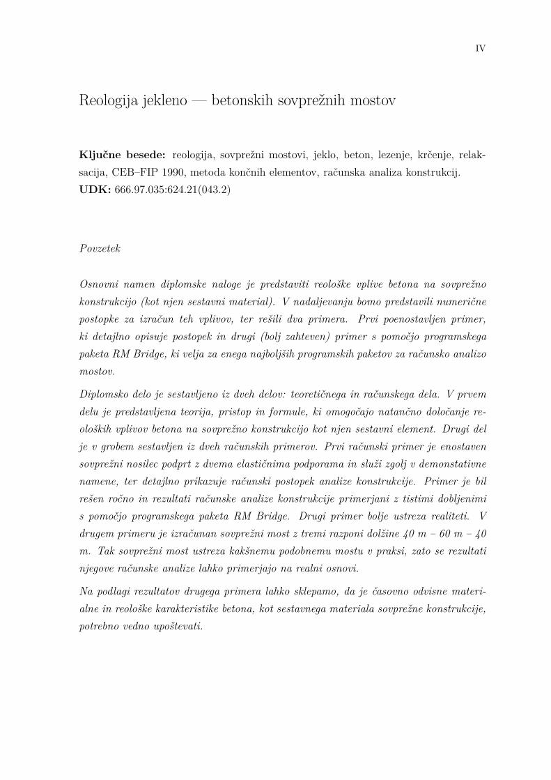
3.1 Introduction
Composite bridges are structures that combine materials such as steel, concrete, timberor masonry in any combination. In common usage nowadays composite constructionis normally conidered as either steel and concrete construction or precast-concrete andin situ concrete bridges. The scope for this work is limited to steel-concrete compositebridges. Steel-concrete composite structures are a common and economical form ofconstruction used in a wide variety of structural types.
3.2 Composite structures in practice
Compliance with codes and regulations is necessary in the design of any structure butis not sufficient for the design of an efficient, elegant and economic structure. Anunderstanding of the structure’s behaviour, in terms of how and why the failure occursis vital to any designer; without this understanding the mathematical equations are ameaningless set of abstract concepts. It is also vital to understand how the structuresare constructed and what is the effect on the stress distribution. One aim of this workis to give a better understanding of the behaviour of composite structures.
Most commonly, steel-concrete composite structures take a simple beam and slab form.However, composite structures are very versatile and can be used for a considerablerange of structures — from foundations, substructures and superstructures through arange of forms from beams, columns, towers and arches, and also for a diverse rangeof bridge structures from tunnels, viaducts, elegant footbridges and major cable-stayedbridges.

Rheology of Steel — Concrete Composite Bridges 9
Steel-concrete composite bridges generally occupy the middle ground between concreteand steel structures; they are competitive with concrete bridges from spans of about20 m in basic beam and slab forms. For heavier loads, as on railways, deeper through-girders or truss forms are more likely. From 50 m to 500 m steel-concrete compositearches and cable-stayed bridges are competitive.
3.3 Materials
The behaviour of the composite structure is heavily influenced by the properties of itscomponent materials. Anyone who wants to understand composite bridges should firsthave a good understanding of the properties and design methods for the individualmaterials. In particular the differences between materials should be noted, as it is theexploitation of these different properties that makes composite construction economic.Concrete has a density of approximately 25 kN/m3, a compressive strength of 30 to100 N/mm2 and almost no tensile strength. Steel has a density of 77 kN/m3, a tensilestrength of 250 to 1880 N/mm2 and is prone to buckling where thin sections are loadedin compression. The use of a concrete slab on a steel girder uses the strength of concretein compression and the high tensile strength of steel to overall advantage.
3.4 Concept design
The first stage in a bridge design is to determine the most economic material, a steel-concrete composite structure may not necessarily be the best form. Cost differencesbetween well-designed all-concrete structures (or even an all-steel structure for longerspans) and steel-concrete composite structures are relatively small. Often the foundingconditions or the nature of the obstacle crossed influences the choice. Where shorterspans can be used and where founding conditions are good a concrete scheme may bebetter. For larger spans or where the lighter deck of a steel concrete composite structureleads to significant savings in pile numbers it is the logical choice. The obstacle crossedmay also dictate certain construction methods, that is launching or cantilevering; theexperience of the contractor building the structure will heavily influence this form.The perceived maintenance regime will also affect the choice: many clients require theadditional costs of the future repainting of steel elements to be taken into account whenconsidering options.

Rheology of Steel — Concrete Composite Bridges 10
Assuming a steel-concrete composite structure is chosen its form must be ascertained.The most simple and common type of steel-concrete composite deck is shown in Fig-ure 4(a). Sometimes in order to try to minimize the number of piers and bearingsof the piers may be inset (Fig. 4(b)); this feature will lead to complex details at di-aphragms, and increase the steelwork tonnage, particularly where piers are at a skew.The intersection of main girders and cross-diaphragms will have issues with lamellatearing and may require a higher quality steel or additional testing. The multi-beamform is relatively simple on straight bridges but can become complex for curved struc-tures. The multi-beam type is also not the most efficient form particularly for widerstructures, as each individual beam has to be designed to carry its share of a heavyabnormal vehicle, leading to more steel in webs and flanges.
The most efficient form of structure for a viaduct is a two-girder system. A number ofvariations on this form are viable, the most common twin girder form being the ladderbeam (Fig. 4(c)), which has two main longitudinal girders with transverse cross-beamsat a longitudinal spacing of 3 to 4 m. Permanent formwork is often used to formthe slab between cross-beams. The forming of the edge cantilevers is often the mostdifficult feature and so the cantilever overhang is generally limited to about 1.5 m.For long spans with deep girders, short cantilevers can be visually distracting. Avariation on the ladder format is to extend the cross-beams beyond the girders to formsteel cantilevers (Fig. 4(d)). This allows the whole deck to be constructed using thepermanent formwork system but will increase steelwork tonnage and can significantlycomplicate fabrication at the girder to cross-beam connection.
Another variation on the twin-girder form is the stringer-beam system (Fig. 4(e)),that reduces the slab span but can increase fabrication complexity because of the trusssystem supporting the stringer. The final variation considered is the plain-girder system(Fig. 4(f)) where the primary steelwork is limited to the main girders with minimumbracing to provide stability. The slab is profiled and designed to carry all the loadsspanning transversely. The slab thickness for this form is greater than the others andso may lead to additional steel tonnage (but not fabrication costs). A formwork gantrysystem would normally be used to form the slab.

Rheology of Steel — Concrete Composite Bridges 11
(a) multi-beam on piers (b) multi-beam with integral crossbead
(c) ladder beam (d) ladder beam with cantilevers
(e) twin beam with stringer beam (f) twin girder
Figure 4: Deck forms

Rheology of Steel — Concrete Composite Bridges 12
3.5 Composite action
There are two primary points to consider when looking at the basic behaviour of acomposite structure:
• The difference in behaviour of the materials
• The connection of the two materials
3.5.1 The modular ratio
Differences between the strength and stiffness of the materials acting compositely affectthe distribution of load in the structure. Stronger, stiffer materials such as steel attractproportionally more load than does concrete. In order to take such differences intoaccount it is common practice to transform the properties of one material into thoseof another by the use of the modular ratio.
At working or serviceability loads the structure is likely to be within the elastic limitand the modular ratio is the ratio of the elastic modulus of the materials.
3.5.2 Interface connection
The connection of the two parts of the composite structure is of vital importance; ifthere is no connection then the two parts will behave independently. If adequatelyconnected, the two materials act as one whole structure, potentially greatly increasingthe structure’s efficiency.
Imagine a small bridge consisting of two timber planks placed one on another, spanninga small stream. If the interface between the two were smooth and no connecting deviceswere provided the planks would act independently, there would be significant movementat the interface and each plank would for all practical purposes carry its own weightand half of the imposed loads. If the planks were subsequently nailed together suchthat there could be no movement at the interface between them then the two partswould be acting compositely and the structure would have an increased section toresist the loads and would be able to carry about twice the load of the non-compositeplanks. The deflections on the composite structure would also be smaller by a factor

Rheology of Steel — Concrete Composite Bridges 13
of approximately 4, the composite whole being substantially stronger and stiffer thanthe sum of the parts.
3.5.3 Shear connectors
Shear connectors are devices for ensuring force transfer at the steel-concrete interface;they carry the shear and any coexistent tension between the materials. Without con-nectors, slip would occur at low stresses. Connectors are of two basic forms, flexibleor rigid. Flexible connectors such as headed studs (Fig. 5) behave in a ductile mannerallowing significant movement or slip at the ultimate limit state. Rigid connectorssuch as fabricated steel blocks or bars behave in a more brittle fashion; failure is eitherby fracture of the weld connecting the device to the beam or by local crushing of theconcrete. In general the capacity of the connectors depends upon a number of vari-ables including the material strength, the stiffness (of the connector, steel girder andconcrete), the width, spacing and height of the connector.
Figure 5: Typical shear connectors types for steel-concrete composite construc-tion, studs, bars with boops and channels

Rheology of Steel — Concrete Composite Bridges 14
3.5.4 State of art
When building short bridges it is possible to design them without bearings or joints. Forlengths up to approximately 80 m it is possible to use integral bridges without joints.For bridges over 80 m long, both joints and bearings are usually used. The bearingsallow the structure to move and accommodate the strains imposed by temperature,creep or shrinkage, without inducing significant stresses. Expansion joints are used atthe ends of the bridge to accommodate this movement and to allow vehicles or trainsto pass over the gap. It is possible to design long bridges without bearings if the pierscan be made flexible enough, for example the 1600 m long Stonecutters Bridge1 has70 m high piers fully built into the deck and no bearings.
Expansion joints and bearings have a lower design life than the main structural ele-ments of the bridge and have to be replaced a number of times over the life of thestructure. The number of joints and bearings should normally be reduced to a min-imum. Proprietary expansion joints and bearings for highway structures can accom-modate movements of ±1000 mm, meaning continuous lengths of viaduct of 2 km arepossible. Railway joints of a similar size to highway joints have been used but tendto be far more complicated and expensive. A maximum length of 1200 m has beenused for recent high-speed lines. A lower length of approximately 80 m is the limit forunjointed continuously welded track. To avoid track joints, railway viaducts are oftenformed from a series of short structures each less than 80 m long.
3.6 Construction sequence and influence of time effects
Since the properties of steel and concrete differ very much, good understanding of theproperties of both materials as well as the interface between both is vital if one wantsto build a composite structure of both materials.
Consider the idealized behaviour of a simply supported composite bridge comprisinga steel beam with a concrete top slab. Initially, on completion of the slab construc-tion, the unpropped steel section only is stressed (at this stage ignoring the effectsof shrinkage) due to self-weight of steel and concrete and there is no force transferat the steel-concrete interface. Loads that are applied after the stage of building the
1For structural analysis of Stonecutters Bridge software package for bridge structural analysis —RM Bridge has been used.

Rheology of Steel — Concrete Composite Bridges 15
composite are the loads that are carried by the whole composite that has differentproperties than starting materials. Therefore stresses in the beam increase, stresses inthe slab occur and there is a force transfer at the steel-concrete interface. The forceat the interface is the rate of change of force along the slab. The load is increased tocause yielding of the bottom flange (to ensure ductile behaviour this must occur priorto concrete crushing). Any further increase of load increases the zone of yield in thebeam until the section becomes fully plastic. Because of the redistribution of stresses,the composite section is now carrying all the load including the steel and concrete self-weight originally carried entirely on the non-composite steel beam. The developmentof stresses is shown in Figure 6.
Figure 6: Stress distribution in composite cross-section in different stages ofconstruction
The behaviour discussed above implicitly assumes that the interface connection doesnot fail or deform significantly prior to failure of the composite section. The connectorsat the interface have their own load deflection behaviour. Any significant movementor slip at the interface will reduce the capacity of the structure.
Where the applied moments cause tension in the concrete, cracking modifies the be-haviour slightly. Consider a cantilever beam with a reinforced concrete top slab. Ini-tially, as before, the steel beam is carrying all of the self-weight. For loads added afterthis stage the composite steel-concrete section carries the load until the tensile capac-ity of the concrete is exceeded. When cracking occurs the section properties changefrom those of the steel-concrete structure to those of the steel beam and the slab re-inforcement only. As the load is increased the steel yields and this ultimately resultsin the formation of a plastic section. Unless there is a significant proportion of steel(4 % or so) the tensile capacity of the slab will be less than its compressive capacity.

Rheology of Steel — Concrete Composite Bridges 16
Consequently, in the cracked section, the force is lower and the rate of change in forceis less and fewer connectors are required in this area. However, at the boundary ofthe cracked to uncracked section of slab there is a more significant change in force andmore connectors are required at this location.
In summary, there are a number of important issues to be noted:
• below the elastic limit the force at the steel-concrete interface is proportional tothe load applied after the composite connection was made
• at failure the force at the steel-concrete interface is proportional to the total loadon the bridge. The force at the interface is the rate of change of force along theslab
• the ultimate strength of the connectors at the interface must be greater than theforces applied at the interface
• the slip at the interface must be small and additional connectors may be requiredat changes of section.
3.7 Construction
For steel-concrete composite bridges the methods and sequences of construction arevitally important. As the concrete is placed, significant stresses are set up in the steel-work. Two basic construction assumptions can be made, that the section is proppedor unpropped.
3.7.1 Propped construction
Propping the steelwork prior to concreting can aid slender or non compact sections. Themajority of load is carried by the composite section immediately the props are removed.For most medium span bridges, the cost of propping is likely to be larger than anysaving in steelwork (from reduced bracing and top flange requirements). Consequentlyit is not often used. On larger span bridges, the potential saving resulting from the useof propping may be more significant and is often worth investigation.

Rheology of Steel — Concrete Composite Bridges 17
3.7.2 Unpropped construction
For unpropped construction, the bridge is built in stages. The steel section initiallycarries the self-weight of steel and concrete with the composite section carrying sub-sequently applied loads. For non-compact sections the stresses induced at each stageof construction should be summed. The sum of these stresses should be less than theallowable for the stage considered.

Rheology of Steel — Concrete Composite Bridges 18
4 CEB–FIP 1990 Model Code
4.1 Introduction
The CEB-FIP Model Code 1990 is the result of a complete revision to the original codeof 1978, which was produced jointly by the Comité Euro-International du Béton - CEB)and the Federation International de la Precontrainte - FIP) and provides comprehensiveguidance to the scientific and technical developments which have occurred over the pastdecade in the safety, analysis and design of concrete structures.
In the following chapters, formulas and procedures from CEB-FIP Model Code 1990will be used. Prediction of time effects of concrete such as development of strength withtime, creep and shrinkage will be based entirely on formulas from the mentioned modelcode.
In addition the variability of creep coefficient and shrinkage strain will be examined,i.e. to determine parameters on which creep and shrinkage depend the most. Basedon the calculation of observed time effects by retaining all the parameters excludingthe time constant that defines creep and shrinkage numerically, the conclusion will bedrawn. From the data presented it will be clearly seen how one particular paramterecan affecth the whole creep and shrinkage and to what extent.
4.2 Development of concrete strength over time
The compressive strength of concrete at the time t depends on the type of cement,temperature and curing conditions. For a mean temperature of 20 ◦C and curing inaccordance with ISO 2736/2 the relative compressive strength of concrete at variousages fcm(t) may be estimated from the following equations:

Rheology of Steel — Concrete Composite Bridges 19
fcm(t) = βcc(t)fcm (4.1)
βcc(t) = exp
⎧⎨
⎩s
⎡
⎣1−(
28t/t1
)1/2⎤
⎦
⎫⎬
⎭(4.2)
tT =n∑
i=1Δti exp
[
13.65− 4000273 + T (Δti)/T0
]
(4.3)
where
fcm(t) . . . mean concrete compressive strength at an age of t daysfcm . . . mean compressive strength after 28 daysβcc(t) . . . coefficient that depends on the age of concrete tt . . . age of concrete (days) that in case of non-average environmen-
tal conditions explained above must be adjusted according toequation (4.3)
t1 . . . 1 days . . . coefficient which depends on the type of cement (for cement
classification, refer to CEB-FIP 1990 Model Code, AppendixD, clause d.4.2.1): s = 0.25 for normal and rapid hardeningcements N and R.
4.3 Development of concrete modulus of elasticity over time
The modulus of elasticity of concrete at an age t �= 28 days may be estimated from thefollowing equations:
Eci(t) = βE(t)Eci (4.4)
βE(t) = [βcc(t)]1/2 (4.5)
where
Eci(t) . . . modulus of elasticity at an age of t daysEci . . . modulus of elasticity at an age of 28 days

Rheology of Steel — Concrete Composite Bridges 20
βE(t) . . . coefficient which depends on the age of concrete, t (days)βcc(t) . . . coefficient according to (4.2)
4.4 Creep and shrinkage
4.4.1 Definitions
The total strain at time t, εc(t), of a concrete member uni-axially loaded at time t0with constant stress σc(t0) may be expressed as follows:
ε(t) = εci(t0) + εcc(t) + εcs(t) + εcT (t) (4.6)
= εcσ(t) + εcn(t) (4.7)
where
εci(t0) . . . initial strain at loadingεcc(t) . . . creep strain at time t > t0εcs(t) . . . shrinkage strainεcT (t) . . . thermal strainεcσ(t) . . . stress dependent strain: εcσ(t) = εci(t0) + εcc(t)εcn(t) . . . stress independent strain: εcn(t) = εcs(t) + εcT (t).
4.4.2 Range of applicability
The prediction mode for creep and shrinkage given below predicts the mean behaviourof concrete cross-section. Unless special provisions are given the model is valid forordinary structural concrete (12 MPa < fck � 80 MPa) subjected to a compressivestress |σc| < 0.4fcm(t0) at an age of loading t0 and exposed to mean temperatures from5 ◦C to 30 ◦C. It is accepted that the scope of the model also extends to concrete intension, though the relations given in the following are directed towards the predictionof creep of concrete subjected to compressive stresses.

Rheology of Steel — Concrete Composite Bridges 21
4.4.3 Creep
(a) Assumptions and related basic equationsWithin the range of service stresses |σv| < 0.4fcm(t0), creep is assumed to be linearlyrelated to stress. For a constant stress applied at time t0 this leads to
εcc(t, t0) = σc(t0)Eciφ(t, t0) (4.8)
where
φ(t, t0) . . . creep coefficientEci . . . modulus of elasticity at the age of 28 days
The stress dependent strain εcc(t, t0) may be expressed as
εcσ(t, t0) = σc(t0)[
1Eci
+φ(t, t0)Eci
]
(4.9)
εcσ(t, t0) = σc(t0)J(t, t0) (4.10)
where
J(t, t0) . . . creep function or creep compliance, representing the totalstress dependent strain per unit stress
Ec(t0) . . . modulus of elasticity at the time of loading t0 according toeq. (4.4); hence 1/Ec(t0) represents the initial strain per unitstress at loading.
For variable stresses or strains, the principle of superposition is assumed to be valid.On the basis of the assumptions and definitions given above, the constitutive equationfor concrete may be written as
εc(t) = σc(t0)J(t, t0) +∫ t
t0J(t, τ)∂σc(τ)
∂τdτ + εcn(t) (4.11)

Rheology of Steel — Concrete Composite Bridges 22
(b) Creep coefficientThe creep coefficient may be calculated from
φ(t, t0) = φ0βc(t− t0) (4.12)
where
φ0 . . . notational creep coefficient eq. (4.13)βc . . . coefficient to describe the development of creep with time after
loading eq (4.19)t . . . age of concrete (days) at the moment consideredt0 . . . age of concrete at loading (days), adjusted according to (4.21)
and (4.3).
The nominal creep coefficient may be estimated from
φ0 = φRHβ(fcm)β(t0) (4.13)
with
φRH = 1 +1−RH/RH0
0.46(h/h0)1/3 (4.14)
β(fcm) =5.3
(fcm/fcm0)0.5 (4.15)
β(t0) =1
0.1 + (t0/t1)0.2 (4.16)
h = 2Ac/u (4.17)
fcm = fck + Δf (4.18)
where
fck . . . characteristic concrete compressive strengthfcm . . . mean compressive strength of concrete at the age of 28 days
(MPa) according to (4.18)

Rheology of Steel — Concrete Composite Bridges 23
fcmo . . . 10 MPaRH . . . relative humidity of the ambient environment ( %)RH0 . . . 100 %h . . . notational size of member (mm) where Ac is the cross-section
and u is the perimeter of the member in contact with theatmosphere
h0 . . . 100 mmt1 . . . 1 day
The development of creep with time is given by
βc(t− t0) =[
(t− t0)/t1βH + (t− t0)/t1
]0.3
(4.19)
with
βH = 150{
1 +(
1.2 RHRH0
)18} h
h0+ 250 � 1500 (4.20)
where
t1 . . . 1 dayRH0 . . . 100 %h0 . . . 100 mm
(c) Effect of type of cement and curing temperatureThe effect of type of cement on the creep coefficient of concrete may be taken intoaccount by modifying the age at loading t0 according to (4.21)
t0 = t0,τ[
92 + (t0,τ/t1,τ )1.2 + 1
]α
� 0.5 days (4.21)
where
t0,τ . . . age of concrete at loading (days) adjusted according to eq(4.3)
t1,τ . . . 1 day

Rheology of Steel — Concrete Composite Bridges 24
α . . . power which depends on the type of cement; α = −1 forslowly hardening cements SL, 0 for normal or rapid hardeningcements N and R, and 1 for rapid hardening high strengthcements RS
4.4.4 Shrinkage
The total shrinkage or swelling strains εcs(t, ts) may be calculated from
εcs(t, ts) = εcs0βs(t− ts) (4.22)
where
εcs0 . . . notational shrinkage coefficient (eq. (4.23))βs . . . coefficient to describe the development of shrinkage with time
(eq. (4.27))t . . . age of concrete (days)ts . . . age of concrete (days) at the beginning of shrinkage or swelling
The notational shrinkage coefficient may be obtainned from
εcs0 = εs(fcm)βRH (4.23)
where
εs(fcm) = [160 + 10βsc(9− fcm/fcm0]× 10−6 (4.24)
where
fcm . . . mean compressive strength of concrete at the age of 28 days(MPa)
fcm0 . . . 10 MPa

Rheology of Steel — Concrete Composite Bridges 25
βsc . . . coefficient which depends on the type of cement: βsc = 4 forslowly hardening cements SL, βsc = 5 for normal and rapidhardening cements N and R, and βsc = 8 for rapid hardeninghigh strength cements RS
βRH =
⎧⎨
⎩
−1.55βsRH for 40 % � RH < 99 %+0.25 for RH � 99 %
⎫⎬
⎭(4.25)
βsRH = 1−(RH
RH0
)3(4.26)
where
RH . . . relative humidity of the ambient atmosphere ( %)RH0 . . . 100 %
The development of shrinkage with time is given by
βs(t− ts) =[
(t− ts)/t1350(h/h0)2 + (t− ts)/t1
]0.5
(4.27)
where
h . . . notational size defined in (4.17)t1 . . . 1 dayh0 . . . 100 mm
4.5 Variability of concrete creep factor
As discussed in this chapter the creep and shrinkage factors depend on numerous pa-rameters. These parameters are mainly geometrical (notational size), material proper-ties and mixture recepies. The question to be answered is, which of mentioned variablesaffect the creep factor the most.
There is no doubt that every material property of concrete is mainly time dependente.

Rheology of Steel — Concrete Composite Bridges 26
To calculate the end creep factor2 we need the following parameters of the construction:
• cross-section properties of the observed concrete member
• projected strength of concrete
• temperature of the surrounding environment
• relative humidity of the surrounding environment
• time of first load appliance
Above defined parameters determine the creep curve. The creep factor can be calcu-lated from the difference of two creep factors at two certain points in time.
For the ease of comparing the dependency of creep and shrinkage curves, the start timeof permanent load will be chosen to be 10 days and the end time to be 10000 days.The difference when choosing various first points for the calculations will be shown anddiscussed in the ending sub-sections of this section. The end creep factor is defined asthe creep or shrinkage factor at the end time.
2Creep factor on the last day in the life of the concrete/composite construction, that is 10000 daysor almost 30 years.

Rheology of Steel — Concrete Composite Bridges 27
4.5.1 Variability of creep factor due to notational size of member
Creep factor also depends on ratio between cross-section area and its perimeter exposedto atmosphere — notational size of member as defined in (4.17).
0 100 200 300 400 500
0
2
4
6
8
notational size of member � h �mm�
cree
pfa
ctor
�Φ�
t,t 0�
Figure 7: Creep factor dependency due to notational size of member
Figure 7 represents the dependence of the creep factor of the member to the ratio ofthe cross-section area to the perimeter of the cross-section exposed to the atmosphere.It can be seen that the creep factor is proportional to that ratio.
4.5.2 Variability of creep factor due to projected concrete strength
As mentioned in section 4.4.2, the CEB-FIP 1990 Model Code covers concrete strengthsfrom 12 to 80 MPa. Due to the fact that every concrete creeps differently, the depen-dency of that strength is shown in Figure 8.
It is an established belief that the hardened concrete develops its strength with time.For normal cements, the time needed to develop almost full projected strength, 28 daysfrom casting the specimen is needed. That 28-day strength is fck.
It can be clearly seen that stronger concretes creep less than weaker ones. To get higherconcrete strength smaller water/cement ratio is needed (drier concrete mixture). Thegraph presented above indicates that the smaller the water/cement ratio the smallerthe creeping of that concrete.

Rheology of Steel — Concrete Composite Bridges 28
20 30 40 50 60 70 80
0.0
0.5
1.0
1.5
2.0
2.5
3.0
3.5
projected concrete strength � fck �MPa�
cree
pfa
ctor
�Φ�
t,t 0�
Figure 8: Creep factor dependency of projected concrete strength
4.5.3 Variation of creep factor with temperature
According to CEB-FIP 1990 Model Code, the temperature is not directly taken intoaccount when calculating the creep factor of a particular member. The temperatureonly affects maturity of the hardened concrete at the moment of the first load.
As presented in (4.3), the temperature adjusted time of first load is clearly defined. Thefollowing figure shows the time dependency of first permanent load with according ofmean temperature of member in time of curing.
5 10 15 20 25 30
�4
�2
0
2
4
6
mean temperature of member �oC�
corr
ectio
ntim
eof
first
load�d
ays�
Figure 9: Creep factor dependency due to mean temperature of member
In the figure 9 the time of first loading of 10 days is taken into consideration. Accordingto (4.3) that time must be corrected due to temperature influence. The CEB-FIP 1990

Rheology of Steel — Concrete Composite Bridges 29
Model Code allows the corrected time to be calculated on the basis of small temperatureincrements. The corrected first time of loading is actually a sum of all temperaturecorrections. To simplify the figure above, only one interval is considered and only onemean temperature interval from 5 ◦C to 30 ◦C, that are most common temperatureswhen building concrete constructions.
If we load the concrete member after 10 days, where the mean temperature of concretemember in that time was 20 ◦C, the corrected time will be the same. If the concretemember mean temperature was only 5 ◦C the corrected time of first loading wouldbe only 5 days. On the other hand, the higher temperature has possitive effect onmaturation of the concrede. If the mean temperature is be 30 ◦C, the concrete wouldmature 15 days in time of 10 days if the temperature would be only 20 ◦C.
4.5.4 Variability of creep factor due to time of first loading
What mostly affects end creep factor is the time of first load appliance. Up to that time,the concrete member develops its projected material characteristics without loading.When observing the time development of elastic modulus, it can be seen that it changesevery day.
1 10 100 1000 1040
1
2
3
4
time of first load appliance � t0 �days�
cree
pfa
ctor
�Φ�
t,t 0�
Figure 10: Creep factor dependency with time of first loading
From Figure 10 it can be seen that the same load applied at the different time in ageof concrete creeps on the different creep curve and produces different end creep. Whendealing with fresh concrete every day has significant impact, whereas old fully developed

Rheology of Steel — Concrete Composite Bridges 30
concrete would at the same circumstances compared to young concrete hardly showany sign of creep at all.
4.5.5 Variability of creep factor due to environment relative humidity
Relative humidity of the surrounding environment of concrete member also plays majorrole. From the following figure it can be seen, that more humid environment workspositively on the creep factor and lowers it.
40 50 60 70 80 90 100
0.0
0.5
1.0
1.5
2.0
2.5
3.0
relative humiditiy of surrounding environment � RH ���
cree
pfa
ctor
�Φ�
t,t 0�
Figure 11: Creep factor dependency due to relative humidity of surroundingenvironment
4.5.6 Summary
In this sub-section one can observe how different independent extrinsic factors influencecreep of concrete. The biggest influence have time of first loading and bundled withthat the maturity of concrete due to mean temperature of curing. The strength ofhardened concrete is in the third place. Weaker concretes creep more than strongerones, basically because of higher water/cement ratio. On the fourth place are thegeometrical properties (notational size). Ratio between cross-section area and cross-section perimeter can however also play a major role in the creep process because ofthe fact that this ratio totally depends on the form of cross section itself.

Rheology of Steel — Concrete Composite Bridges 31
4.6 Variability of concrete shrinkage
In contrary to creep, shrinkage of concrete is stress independent variable. Creep factoris a scalar with which elastic deformation has to be multipied with in order to get
The shrinkage factor represents shrinkage strain, the quantity that is stress indepen-dent. However, it depends on some other material properties of concrete such asrelative humidity of the surrounding environment (atmosphere in contact with surfaceof the concrete), geometry (notational size), material properties and composition ofthe mixtures. It is discussable which of the given variables has the biggest effect onthe shrinkage strain.
To calculate end shrinkage strain the following parameters of the construction areneeded:
• cross-section properties of the observed concrete member
• projected concrete strength
• relative humidity of the surrounding environment
• beginning of shrinkage

Rheology of Steel — Concrete Composite Bridges 32
4.6.1 Variability of shrinkage due to notational size of member
Like creep, shrinkage strain also depends on the ratio between cross-section area andits perimeter exposed to atmosphere as defined in (4.17).
0 100 200 300 400 500�600
�500
�400
�300
�200
�100
0
notational size of member � h �mm�
shri
nkag
est
rain
�� c
s�m
icro
stra
in�
Figure 12: Shrinkage strain dependency of notational size of member
The smaller the ratio between cross-section area and the perimeter exposed to envi-ronmental atmosphere, the greater the shrinkage. A concrete slab with proportionsb/h = 10/1 would shrink only half the amount as would a column with proportionsb/h = 1/1.
4.6.2 Variability of shrinkage strain due to mean concrete strength
Shrinkage highly depends also on the projected strength of concrete. Concretes withlower strength shrink more than those with higher strength.. The model code CEB-FIP1990 covers concrete strengths from 12 to 80 MPa. The variability of shrinkage due tothat projected strength can be seen in figure 13.
Reason for increased shrinkage due to lower concrete strength can be ascribed to, likewith creep, greater water/cement ratio of fresh concrete mixture. Concretes with higherstrength require lower water/cement ratios.

Rheology of Steel — Concrete Composite Bridges 33
10 20 30 40 50 60 70 80
�700
�600
�500
�400
�300
�200
�100
0
mean compressive strength of concrete after 28 days � fcm �MPa�
shri
nkag
est
rain
�� c
s�m
icro
stra
in�
Figure 13: Shrinkage strain dependency of mean concrete strength
4.6.3 Variability of shrinkage strain due to relative humidity of surround-ing environment
Relative humidity of the air that is in contact with the observed concrete memberhas the most significant impact on the shrinkage. CEB-FIP 1990 Model Code covershumidities from 40 to 99 % and above. This range is also most common in the lifespanof concrete construction — observed concrete member.
40 50 60 70 80 90 100
�600
�500
�400
�300
�200
�100
0
relative humidity of surrounding environment � RH ���
shri
nkag
est
rain
�� c
s�m
icro
stra
in�
Figure 14: Shrinkage strain dependency from relative humidity of surroundingenvironment
If air in contact with surface of the concrete is dry, water that is not chemically boundcan easily evaporate from the concrete. Because of the geometrical factors concretedries irregularly and inhomogeneously. Part of concrete that is closer to the sirface or

Rheology of Steel — Concrete Composite Bridges 34
in contact with atmosphere will dry faster than part that is deeper and further fromthe surface.
4.6.4 Variability of shrinkage strain due to time of shrinkage start
In contrast to creep creep, the actual start of shrinking process has a small influenceon the end shrinkage strain. Whereas the creep factor would be significantly differentif the first loading is applied a day later, the shrinkage does not show that kind ofdependence. As seen in the Fig. 15 shrinkage that starts at day 10 or 20 gains fasterthan that started on day 2. In the end, day of shrinkage start – ts has almost no effectat all.
1 10 100 1000 104�600
�500
�400
�300
�200
�100
0
time of shrinkage start � ts �days�
shri
nkag
est
rain
�� c
s�m
icro
stra
in�
Figure 15: Shrinkage strain dependency from shrinkage start
4.6.5 Summary
Relative humidity of surrounding environment and the mean strength of concrete usedhave the biggest impact on the shrinkage of the concrete. The second most importantpart plays the notational size of member (term explained in (4.17). That factor caninfluence the shrinkage to almost 50 % but can also deliver unpredictable results dueto the fact, that the cross-section geometry can be complex in such manner that theformulae do not comply anymore.

Rheology of Steel — Concrete Composite Bridges 35
5 Numerical prediction of creep and shrinkage
5.1 Primary, secondary and total forces
Figure 16: Primary effects in concrete/steel composite section
In the case of composite beam it is not important whether the beam is supportedin statically indeterminate or determinate way, because the nature of the composite(composed of two or more dissimilar materials joined together to act as a unit) alreadydefines it to be indeterminate. Two materials that have different time dependantcharacteristics are prone to develop additional inner forces.
Shrinkage is in fact very similar to temperature load. Because of the fact, that incomposite none of the parts can deform separately, the shrinkage of the concrete partwill cause additional inner primary forces in both steel and concrete. The concretepart tends to deform, whether the steel part counteracts this deformation partially bydeforming only to some extent. Metaphorically speaking an agreement between thesetwo parts is made and the deformation of the composite due to shrinkage in concreteis somewhere between no deformation in steel at all and free deformation of concretepart itself. Deformations of both parts are then in equilibrium. Concrete is from the

Rheology of Steel — Concrete Composite Bridges 36
perspective of free deformation pulled apart and steel compressed together.
The basics explained above are valid for creep as well. The difference between creepand shrinkage is in stress dependency, Creep in contrast to shrinkage is stress depen-dent. Therefore creep and shrinkage in concrete part of the composite always produceprimary and sometimes also secondary forces in the whole composite.
Most commonly the observed member is a part of some larger construction. Whensome intrinsical factor like temperature, shrinkage or creep is changed the membershrinks/expands forcing the surrounding construction to deform accordingly. Themember itself pushes/pulls with primary force, construction reacts with secondary atthe same time relieving the primary. To predict time effects that depend on the forcein member the real magnitude of force in the material must be determined. That wayanother force is needed.
Total forces resemble the summation of primary and secondary forces per material.Total forces represent the real amount of force that can only be used in predictingstress dependent time effects in concrete.
For demonstration of the abovementioned forces Example 1 in this work can be con-sulted.

Rheology of Steel — Concrete Composite Bridges 37
5.2 Age-adjusted modulus of elasticity
The three terms in Equation (5.1) represent the strain in concrete at age t due to:a stress σc(t0) introduced at age t0 and sustained during the period (t − t0), a stressincrement of magnitude zero at t0, increasing gradually to a final value Δσc(t) at aget and the free shrinkage occurring during the period (t − t0). This equation may berewritten as follows:
εc(t) = σc(t0)1 + φ(t, t0)Ec(t0)
+ Δσc(t)E∗c (t, t0)
+ εcs(t, t0) (5.1)
where
E∗c (t, t0) =Ec(t0)
1 + χφ(t, t0)(5.2)
E∗c (t, t0) is the age-adjusted elasticity modulus to be used in the calculation of the totalstrain increment, instantaneous plus creep, due to the stress increment of magnitudedeveloping gradually from zero to a value Δσc(t). Thus, the strain increment in theperiod (t− t0) caused by the stress Δσc(t) is given by:
Δεc(t) =Δσc(t)E∗c (t, t0)
(5.3)

Rheology of Steel — Concrete Composite Bridges 38
5.3 Stepping in the time domain
5.3.1 Linear time stepping
The numerical solution is accomplished step by step in the time domain. Let time t1correspond to the start and time t2 to the end of a given time step. It can be assumedthat complete load/response history is known (including all stress increments) fromtime equal to zero up to the start (time t1) of the time step. Basic unknowns arestresses and strains (or corresponding integral forces and displacement) at the end oftime step (time t2).
ε2 = ε1 + Δε (5.4)
where
Δε =∫ t2
t1
∂ε
∂tdt (5.5)
(5.6)
σ2 = σ1 + Δσ (5.7)
where
Δσ =∫ t2
t1
∂σ
∂tdt (5.8)
The total strain increment Δε can be divided into elastic and plastic part. It can beassumed that elastic strain depends linearly on the stress state.
Δε = Δεe + Δεp (5.9)
The total plastic strain increment consists of three parts.
Δε =n∑
i=1
∫ t2
t1
σiE
∂φi(t)∂tdt+
∫ t2
t1
∂εs∂tdt+
∫ t2
t1
1E
∂σ
∂τ(1 + φ∗(τ, t)) dτ (5.10)
The first part is a plastic strain increment due to the creep of all stress incrementsoccurring before time t1. The second part is a plastic strain increment due to shrinkage

Rheology of Steel — Concrete Composite Bridges 39
of concrete. Those two terms are basically known and can be evaluated in closed form atany time t. The third part of the plastic strain is produced by creep of additional elasticstrain increments which continuously occur within the time step (between time t1 andtime t2). This part together with corresponding elastic strain increment is unknownand needs to be determined. It is obvious that the third integral term produces majordifficulties. Instead of determining the continuous change between time t1 and timet2 it is advantageous to look only for the final solution at the end of the time step(at time t2). Linear change of elastic strain within time step according to the “finitedifferences” theory will be assumed.
ε = w1ε1e + w2ε
2e (5.11)
1 = w1 + w2 (5.12)
Figure 17: Elastic strain increment and creep coefficient over time
Additionally it can be assumed that the third integrand can be approximated by thefollowing simplified term:
∫ t2
t1
1E
∂σ
∂τ(1 + φ∗(τ, t)) dτ ≈ (1 + φw)
∫ t2
t1
1E
∂σ
∂τdτ (5.13)
The final expression is then given by:
Δε =n∑
i=1
σiE
(εi(t2)− εi(t1)) + (εs(t2)− εs(t1)) + (1 + Φw)ΔσE
(5.14)
The solution is now straightforward. There are two basic possibilities. The first optionis to establish the new stress/strain relation using an equivalent elastic modulus and

Rheology of Steel — Concrete Composite Bridges 40
solving by stress increment. This solution is very elegant but has the disadvantagethat it cannot be combined with further non-linear effects like p-delta effects, largedisplacements etc. A more appropriate solution is to iterate the corresponding plasticstrain due to the additional elastic strain increment within a general Newton/Raphsonprocedure. This solution is implemented in the software package RM Bridge in a closedand consistent algorithm. However both solutions lead to same results.
5.3.2 Logarithmic time stepping
The described solution in the time domain has an approximate nature. The numberof time steps has to be increased in order to get a more accurate solution, as commonin classical FEM3.
The use of equal time steps is inappropriate because creep functions have an exponen-tial characteristic. Therefore it is useful to make equal time steps in the logarithmictime domain. Experience has shown that the calculation of end creep (up to timeinfinity) can be done using 3 — 4 time steps in the logarithmic time domain. Smallercreep intervals within the construction schedule only need (on average) one time step.Bending moment due to the final creep can have differences of about 12 % to 18 %between solution with 1 time step and 3 logarithmic sub-steps.
�T 1 �T 2 �T 3
�T
0 20 40 60 80 1000.0
0.5
1.0
1.5
2.0
2.5
3.0
time �days�
cree
pfa
ctor
Figure 18: Logarithmic subdivision of time step into three sub steps
3FEM — Finite Element Method

Rheology of Steel — Concrete Composite Bridges 41
6 Software package RM Bridge
6.1 Software capabilities and introduction
RM Bridge is a comprehensive structural engineering, design and analysis system,developed by TDV GmbH which was recently acquired by Bentley Systems Inc. It canhandle virtually any type of bridge — from simple segmented and complex cable-stayedthrough to suspension bridges and long crossings.
Some of the bridges designed using the software are setting new records for bridgeconstruction. The cable-stayed Stonecutters Bridge in Hong Kong, at 1018 metres, isthe first to have a main span exceeding 1000 metres. That will soon be exceeded bythe Hardanger Suspension Bridge in Norway, with a main span of 1310 metres. TheSutong Bridge, which will cross the Yangtse river, will stretch for 8206 meters, and willinclude a multi-span cable-stayed section of 1088 metres. And, in America, they havebuilt two side-by-side Bascule bridges, each 1852 metres long.
Bentley’s RM Bridge provides a series of highly sophisticated linear and non-linearanalysis modules for all bridge types and construction sequences, with built-in timedimension, parametric geometry definition and integrated tendon design. It can han-dle segmental construction loading, stage construction and erection control, stochasticwind event design, CFD, wind tunnel simulation and other modules.

Rheology of Steel — Concrete Composite Bridges 42
When you are trying to bridge a 1000-plus metre gap, balancing the constructionsequence with the load on the extending span requires the deftest of touches from acomplex piece of mathematical engineering. The inclusion of a number of CFD andwind testing modules in the solution also indicate just how much prevalent weatherconditions affect the design. There have been some notable bridge disasters in the pastthat happened entirely due to adverse weather conditions. Besides wind, designersalso have to contend with water - extreme tides and fast currents - and bridge traffic,especially the vibrational and other effects from high-speed carrying trains.
Consequently, a number of international design codes have been set up, which are allfully supported by RM Bridge, including AASHTO Load and Resistance Factor Design(LRFD) Bridge Specifications. The software carries out specific SLS and ULS designcode checks in accordance with these 14 international standards.
RM Bridge allows bridge designers to model structures in 3D, with a CAD-style geo-metric pre-processor that enables designers to define the structural model of a bridge.Complex bridge geometry is developed in plan and elevation by defining axes, using thesame type of geometric elements used in road construction (straight, circular, parabolic,spiral etc.) and building the superstructure by placing different cross-sections alongthese axes. The different segments relate to the physical model as elements and nodes.Again, harking back to the way that the bridges are actually built, special types ofsegments have to define the temporary support conditions in incremental launchingprocesses (ILM segments). Other segment types include cross-girders of truss models(link segments) and substructure entities, such as abutments, piers or pile groups. The3D model of the bridge can actually be 4D, as it can be used to simulate the erec-tion process using a time axis in the calculation — vital in the segmental constructionloading and erection control processes. And there are no limits to the type of bridgethat can be built using RM Bridge, nor to the erection sequence — bar that of physi-cal impossibility! The program is in use by many international consultants and a fewthousand bridges worldwide have been designed using this powerful engineering tool.
RM Bridge includes a sophisticated CFD module, based on the vortex particle method,to handle its dynamic wind analysis throughout the whole process. It includes FiniteElement Modelling, also integrated within its erection control facility, which not onlyallows full non-linear analysis for all types of bridge structures but also contains specialdesign check modules for proof-checking, stability and serviceability.

Rheology of Steel — Concrete Composite Bridges 43
These functions include ultimate load checking for reinforced and/or pre-stressed mem-bers, shear checks and robustness checks. The checking modules include reinforcementdesign functions that can determine whether additional reinforcement is needed any-where on the bridge structure.
Stay cable stressing looks more like tuning a grand piano, creating or evaluating a staycable stressing sequence to reach a given maximum stress state in the superstructure,is all a matter of optimisation of the stresses on both permanent and temporary staycables.
The RM Bridge algorithms for the process work out the tensioning of each single cable,first as a unit load case taking into account the current structural system and theninfluencing all previously applied unit load cases. All other loadings (self weight of thenew segment, moving the traveller etc.) related to the individual erection procedureare also calculated step by step.
Recently, Bentley has concentrated a lot of effort on improving its dynamic analysiscapability, taking it beyond standard forced vibration and earthquake-response anal-ysis. This allows the software to cater for high-speed railway systems using bridges,taking into account moving loads as well as moving masses, and sophisticated dynamicwind analysis on the ultra long bridges.

Rheology of Steel — Concrete Composite Bridges 44
6.2 Some Composite bridges designed with use of RM Bridge
• Tähtiniemi Bridge, Finland:Leonhardt, Andrä & Partner, Germany:Cable-stayed bridge, cross section is composite construction (steel+concrete) with12 spans, total length 901 m.
• Kap Shui Mun Bridge, Hong Kong:Leonhardt, Andrä & Partner, Germany:Cable-stayed bridge, cross section is composite construction (concrete + steel),main span 430 m.
• Sunningesund-Bridge, Sweden:Johs Holt A.S., Norway:Cable-stayed bridge with composite cross section (concrete + steel), main span414 m, total length of bridge 1712 m.
• Verige Bridge, Montenegro:Gradis, Slovenia:Balanced cantilevering method, concrete deck and composite pylon, main span450 m, total length of bridge 980 m.
• Kao Ping Hsi-Bridge, Taiwan:VCE — Fritsch — Chiari, Taiwan:Cable-stayed bridge with composite cross section (concrete + concrete) and steelbox, main span 330 m.
• Valley Bridge – Reichenbach, Germany:FCP Fritsch — Chiari & Partner, Austria:Fourteenspan composite bridge — steel girder, concrete deck, total length 1000m.

Rheology of Steel — Concrete Composite Bridges 45
7 Example 1 — composite girder on elastic sup-ports
7.1 Introduction
Figure 19: Picture of cross-section and the structural system
In this example a simple composite girder is presented. It is composed of top concreteC35/45 slab and bottom IPE 500 S355 steel beam girder. That composite beam has aspan of 8 meters and is spanned left with a spring K1 and right with spring K2.
After 10 days from casting the top slab, the first loading case is applied. This firstloading case consists of bending load (Figure 19: M1 and M2) on each end of thecomposite girder. The result of that loading case will be constant bending momentthrough the whole length of the composite girder.
The second loading case is applied 20 days after the first loading case. That secondloading consists only of a horizontal force (Figure 19: F2) that is applied on the right endof composite girder in the way that it causes constant axial load and bending momentdue to force application eccentricity throughout the whole length of the girder.

Rheology of Steel — Concrete Composite Bridges 46
(a) time = 10 days: loading case 1:Constant bending moment
(b) time = 10 — 30 days: creep andshrinkage 1
(c) time = 30 days: loading case 2:Constant axial force and bending
moment
(d) time = 30 — 10000 days: creep andshrinkage 2
Figure 20: Construction stages

Rheology of Steel — Concrete Composite Bridges 47
For the purpose of simplicity, the module of elasticity of concrete is taken as constantand not a time dependent variable. Creep and shrinkage functions are also simplified toonly approximate the shape of a real creep function and therefore calculation of themin this example is not needed. All this simplifications are made for we can focus inthe main part of the problem, i.e. observing the deformations of the composite girder,rebalancing of inner structural forces in concrete, steel and the rest of the constructionand, most importantly, observing the effect called creep of creep.
Our interval for observation is from the creation of the composite girder to the age of10000 days (almost 30 years).
7.2 Cross-section and material data
Esteel = 2.1× 10⁸ kN
m2
Econc = 3.4× 10⁷ kN
m2
Asteel = AIPE500 = 115.53 cm2
Aconc = 150 cm× 20 cm = 3000 cm2
where
Esteel . . . Module of elasticity of steel part of compositeEconc . . . Module of elasticity of concrete part of compositeAsteel . . . Cross-section area of the steel part of compositeAconc . . . Cross-section area of the concrete part of composite

Rheology of Steel — Concrete Composite Bridges 48
7.3 Creep and shrinkage function for concrete
To simplify this example in great manner, a calculation of actual creep curve for con-crete used in this example will be omitted. Instead, creep function from section 4.5and shrinkage function from 4.6 will be used and their coefficients slightly corrected.
φ(t, t0) =5(t−t0
700+t−t0)0.3
0.1 + t0.20(7.1)
εcs(t, ts) = −0.0006(
t− ts40000130 + t− ts
)0.5
(7.2)
where
φ(t, t0) . . . simplified creep function of concrete that will be used through-out the whole example
εcs(t, ts) . . . simplified shrinkage function of concrete that will be usedthroughout the whole example
7.4 Stiffness matrices of the elements and structural system
In this sub-section we will calculate the stiffness matrices for each individual elementof construction and subsequently of the whole structural system itself. That particularmatrices can then be used in every particular loading case.
7.4.1 Stiffness matrices of spring elements
Element nameLocal stiffnesses of springs
X – stiffness: Kx,n Y – stiffness: Ky,n ϕ – stiffness: Kϕ,nLeft spring – K1 108 108 104
Right spring – K2 108 0 104
Table 1: Stiffness coefficients of spring elements
Local stiffness matrix of a spring element:

Rheology of Steel — Concrete Composite Bridges 49
[
KLs,n]
=
⎡
⎢⎢⎢⎢⎢⎢⎢⎢⎢⎢⎢⎢⎢⎣
Kx,n 0 0 −Kx,n 0 00 Ky,n 0 0 −Ky,n 00 0 Kϕ,n 0 0 −Kϕ,n−Kx,n 0 0 Kx,n 0 0
0 −Ky,n 0 0 Ky,n 00 0 −Kϕ,n 0 0 Kϕ,n
⎤
⎥⎥⎥⎥⎥⎥⎥⎥⎥⎥⎥⎥⎥⎦
(7.3)
Rotation matrix for rotating an element around global Z – axis:
[Rα] =
⎡
⎢⎢⎢⎢⎢⎢⎢⎢⎢⎢⎢⎢⎢⎣
cos (α) sin (α) 0 0 0 0−sin (α) cos (α) 0 0 0 0
0 0 1 0 0 00 0 0 cos (α) sin (α) 00 0 0 −sin (α) cos (α) 00 0 0 0 0 1
⎤
⎥⎥⎥⎥⎥⎥⎥⎥⎥⎥⎥⎥⎥⎦
(7.4)
Definition for transformation (rotation and translation) of a beam element:
Figure 21: local and global coordinate system
{Fglobal} = [R]× {Flocal} (7.5)
[Kglobal] = [R]T × [Klocal]× [R] (7.6)

Rheology of Steel — Concrete Composite Bridges 50
Spring on the left end of the composite girder – Spring 1 is oriented towards north.The angle of rotation for the rotational transformation – α is then equal to 90 degreescounterclockwise. Transformation of Spring 1 from local to global coordinate system:
[
KGs,1]
= [R90◦ ]T ×[
KLs,1]
× [R90◦ ]
[
KGs,1]
=
⎡
⎢⎢⎢⎢⎢⎢⎢⎢⎢⎢⎢⎢⎢⎣
108 0 0 −108 0 00 108 0 0 −108 00 0 104 0 0 −104
−108 0 0 108 0 00 −108 0 0 108 00 0 −104 0 0 104
⎤
⎥⎥⎥⎥⎥⎥⎥⎥⎥⎥⎥⎥⎥⎦
Spring on the right end of the composite girder – Spring 2 is oriented toward south. Theangle of rotation – α in this case is 90 degrees clockwise or – 90 degrees counterclockwise.
[
KGs,2]
= [R−90◦ ]T ×[
KLs,1]
× [R−90◦ ]
[
KGs,2]
=
⎡
⎢⎢⎢⎢⎢⎢⎢⎢⎢⎢⎢⎢⎢⎣
108 0 0 0 0 00 108 0 0 −108 00 0 104 0 0 −104
0 0 0 0 0 00 108 0 0 108 00 0 −104 0 0 104
⎤
⎥⎥⎥⎥⎥⎥⎥⎥⎥⎥⎥⎥⎥⎦

Rheology of Steel — Concrete Composite Bridges 51
7.4.2 Stiffness matrix of the composite girder
For numerical purpose we can assign material to composite section. However, this isonly “equivalent” material for analysis.
Figure 22: Explanation of geometrical values of cross-section
First we have to calculate the area, position of centroid and the moment of inertia ofthe whole composite cross-section. This is basically the area of a fictional cross-sectionthat composes out of only one material, in our case steel. This is only theoreticalapproach. In reality, however, there is no such thing as a composite girder.
Acomp = Asteel × Esteel + Aconc × EconcEcomp
= 601.244 cm2
where
Acomp . . . fictional area of composite cross-sectionEcomp . . . modulus of elasticity of composite; Ecomp = Esteel
Eccentricity – position of the composite centroid. Values of ecomp matches the distancefrom the bottom of the composite cross-section to the centroid itself4.
4RM Bridge uses more general matrix approach. Here we use only classic approach.

Rheology of Steel — Concrete Composite Bridges 52
ecomp =Asteel × Esteel × Hsteel2 + Aconc ×Econc × (Hsteel + Hconc
2 )Asteel × Esteel + Aconc × Econc
ecomp = 53.275 cm2
Distance from composite centroid to local concrete centroid:
econc = Hsteel +Hconc
2− ecomp = 6.725 cm
where
Hsteel . . . height of steel cross-sectionHconc . . . height/thickness of the concrete slab
Distance from composite centroid to local steel centroid:
esteel =Hsteel
2− ecomp = −28.274 cm
Moment of inertia of the equivalent composite cross-section (Steiner’s law):
Icomp =(Isteel + Asteel × e2steel)× Esteel + (Iconc + Aconc × e2conc)×Econc
Ecomp
Icomp = 178724.6 cm4
Stiffness matrix for composite in local coordinate system for composite girder (classicalbeam theory without shear deformations). Note: Due to the paper size limitations theindexes of geometrical properties are (only in the next matrix) even further abbreviatedfrom “comp” to “c”.

Rheology of Steel — Concrete Composite Bridges 53
[
KLc]
=
⎡
⎢⎢⎢⎢⎢⎢⎢⎢⎢⎢⎢⎢⎢⎣
−Ec×IcL
0 0 −Ec×IcL
0 00 12×Ec×Ic
L3 −6×Ec×IcL2 0 −12×Ec×Ic
L3 −6×Ec×IcL2
0 −6×Ec×IcL2
4×Ec×IcL
0 6×Ec×IcL2
2×Ec×IcL
−Ec×IcL
0 0 Ec×IcL
0 00 −12×Ec×Ic
L3 −6×Ec×IcL2 0 12×Ec×Ic
L36×Ec×IcL2
0 6×Ec×IcL2
2×Ec×IcL
0 6×Ec×IcL2
4×Ec×IcL
⎤
⎥⎥⎥⎥⎥⎥⎥⎥⎥⎥⎥⎥⎥⎦
The orientation of the local coordinate system of the composite coincides with theglobal coordinate system so that rotational conversion of the local stiffness matrix isnot necessary in this case. The origin on the other hand does not. We have to createa rigid link between the local composite centroid axis and the left and right springendings that are connected to global composite axis that lie on the bottom of thecomposite member/cross-section and not in the centroid like in the given case.
Transformation matrix – rigid link in length of “e”:
[Te] =
⎡
⎢⎢⎢⎢⎢⎢⎢⎢⎢⎢⎢⎢⎢⎣
1 0 e 0 0 00 1 0 0 0 00 0 1 0 0 00 0 0 1 0 e0 0 0 0 1 00 0 0 0 0 0
⎤
⎥⎥⎥⎥⎥⎥⎥⎥⎥⎥⎥⎥⎥⎦
(7.7)
Global stiffness matrix for composite:
[
KGcomp]
= [Tec ]T × [R0◦]T ×
[
KLcomp]
× [R0◦] [Tec ]
[
KGcomp]
=
⎡
⎢⎢⎢⎢⎢⎢⎢⎢⎢⎢⎢⎢⎢⎣
1578266 0 840817 −1578266 0 −8408170 8797 −35186 0 −8797 −35186
840817 −35186 635603 −840817 35186 −354112−1578266 0 −840817 1578266 0 840817
0 −8797 35186 0 8797 35186−840817 −35186 −354112 840817 35186 635603
⎤
⎥⎥⎥⎥⎥⎥⎥⎥⎥⎥⎥⎥⎥⎦
After we calculated each members stiffness matrix, we can calculate the structure

Rheology of Steel — Concrete Composite Bridges 54
stiffness matrix. Stiffnesses that coincide in manner of degrees of freedom are addedup respectively.
[Ksys] =[
KGs,1]
+[
KGC]
+[
KGs,2]
Our system has total of twelve degrees of freedom. Six out of twelve degrees are totallyfixed and we know that the movement there is zero. Reduced stiffness matrix from thewhole system is:
[
KRsys]
= [Ksys]{4−9,4−9}
[
KRsys]
=
⎡
⎢⎢⎢⎢⎢⎢⎢⎢⎢⎢⎢⎣
100989139 0 487340 −989139 0 −4873400 100007631 −30525 0 −7631 −30525
487340 −30525 412908 −487340 30525 −158709−989139 0 −487340 989139 0 487340
0 −7631 30525 0 100007631 30525−487340 −30525 −158709 487340 30525 412908
⎤
⎥⎥⎥⎥⎥⎥⎥⎥⎥⎥⎥⎦

Rheology of Steel — Concrete Composite Bridges 55
7.5 Loading case 1 — LC1: Constant bending moment
On day 10 from casting the concrete part of the composite member load is appliedon the composite girder for the first time. Load consists of nodal bending moment of500 kNm on the both ends of the composite girder. Loading vector5 with respect toreduced (or free) degrees of freedom thereby is:
{F} =
⎧⎪⎪⎪⎪⎪⎪⎪⎪⎪⎪⎪⎪⎪⎨
⎪⎪⎪⎪⎪⎪⎪⎪⎪⎪⎪⎪⎪⎩
00
50000−500
⎫⎪⎪⎪⎪⎪⎪⎪⎪⎪⎪⎪⎪⎪⎬
⎪⎪⎪⎪⎪⎪⎪⎪⎪⎪⎪⎪⎪⎭
Movement of free nodes by their degrees of freedom due that loading vector:
{u} =[
KRsys]−1 × {F} =
⎧⎪⎪⎪⎪⎪⎪⎪⎪⎪⎪⎪⎪⎪⎨
⎪⎪⎪⎪⎪⎪⎪⎪⎪⎪⎪⎪⎪⎩
00
4.815 rad5.131 m
0−4.815 rad
⎫⎪⎪⎪⎪⎪⎪⎪⎪⎪⎪⎪⎪⎪⎬
⎪⎪⎪⎪⎪⎪⎪⎪⎪⎪⎪⎪⎪⎭
× 10−3
5Note: different sign because of FEM notation

Rheology of Steel — Concrete Composite Bridges 56
Forces in composite:
{F compfem } =[
KLcomp]
× [Tecomp]× {u} =
⎧⎪⎪⎪⎪⎪⎪⎪⎪⎪⎪⎪⎪⎪⎨
⎪⎪⎪⎪⎪⎪⎪⎪⎪⎪⎪⎪⎪⎩
0 kN0 kN
451.845 kNm0 kN0 kN
−451.845 kNm
⎫⎪⎪⎪⎪⎪⎪⎪⎪⎪⎪⎪⎪⎪⎬
⎪⎪⎪⎪⎪⎪⎪⎪⎪⎪⎪⎪⎪⎭
where
{F compfem } . . . vector of inner forces in finite element method coordinate sys-tem — notation
[
KLcomp]
. . . stiffness of composite girder in his local coordinate system[
Tecomp]
. . . transformation/translation matrix for composite girder, fromglobal coordinate system to local composite coordinate system
(a) Finite element method notation
(b) Finite element beam notation
Transformation of inner forces from finite element method notation to finite elementbeam notation (only bending moment and axial force):
⎧⎨
⎩
N
M
⎫⎬
⎭
comp
1
=
⎡
⎣1 00 −1
⎤
⎦× {F femcomp}1,3 =
⎧⎨
⎩
0 kN451.845 kNm
⎫⎬
⎭
⎧⎨
⎩
N
M
⎫⎬
⎭
comp
2
=
⎡
⎣1 00 −1
⎤
⎦× {F femcomp}4,6 =
⎧⎨
⎩
0 kN451.845 kNm
⎫⎬
⎭
where

Rheology of Steel — Concrete Composite Bridges 57
N compi . . . axial force at node i in compositeM compi . . . bending moment at node i in composite
Due to the symmetry of loading we can make one more simplification. The fact thatN comp1 and N comp2 or M comp1 and M comp2 are the same, in the continuation only N comp∗or M comp∗ will be used. The same goes for similar symbols.
Inner forces cause strain in composite at cross-section level. To calculate the strainwe need the elasticity matrix — Q of composite. Strain in node 1 (left end of thecomposite girder as shown in Figure 19) and node 2 (right end of the composite):
[
QLcomp]
=
⎡
⎣Acomp × Ecomp 0
0 Icomp ×Ecomp
⎤
⎦
[
QLcomp]
=
⎡
⎣12626130 kN 0
0 375321 kNm2
⎤
⎦
Strain in composite due LC1:
Figure 23: Strain at cross – section level
⎧⎨
⎩
ε
κ
⎫⎬
⎭
comp
=[
QLcomp]−1 ×
⎧⎨
⎩
N
M
⎫⎬
⎭
comp
=
⎧⎨
⎩
01.2039
⎫⎬
⎭× 10−3
where
εcomp . . . strain of composite cross-section on the center og ravity axisκcomp . . . difference in angle of strain plane

Rheology of Steel — Concrete Composite Bridges 58
7.5.1 Primary forces
Primary forces in this particular loading case are expected to be zero. Outer loadingcannot cause primary forces.
⎧⎨
⎩
N
M
⎫⎬
⎭
conc
prim
=
⎧⎨
⎩
N
M
⎫⎬
⎭
steel
prim
=
⎧⎨
⎩
0 kN0 kNm
⎫⎬
⎭
7.5.2 Secondary forces
Forces in concrete at cross – section level
Elasticity matrix of concrete part of composite – Qconc,
[
QLconc]
=
⎡
⎣Aconc × Econc 0
0 Iconc × Econc
⎤
⎦ =
⎡
⎣10200000 kN 0
0 34000 kNm2
⎤
⎦
transformation of deformation from local composite coordinate system to local concretecoordinate system.
Figure 24: conversion from local concrete coordinate system to local compositecoordinate system
⎧⎨
⎩
ε
κ
⎫⎬
⎭
conc
=
⎡
⎣1 −econc0 1
⎤
⎦×⎧⎨
⎩
ε
κ
⎫⎬
⎭
comp
=
⎡
⎣6.48539−96.4327
⎤
⎦× 10−6

Rheology of Steel — Concrete Composite Bridges 59
and finally secondary forces in concrete part.
⎧⎨
⎩
N
M
⎫⎬
⎭
conc
sec
= [Qconc]×⎧⎨
⎩
ε
κ
⎫⎬
⎭
conc
=
⎧⎨
⎩
−825.843 kN40.932 kNm
⎫⎬
⎭
Secondary forces in steel part of the composite girder
Elasticity matrix of steel part of composite – Qsteel,
[
QLsteel]
=
⎡
⎣Asteel ×Esteel 0
0 Isteel × Esteel
⎤
⎦ =
⎡
⎣10200000 kN 0
0 34000 kNm2
⎤
⎦
transformation of deformation from local composite coordinate system to local steelcoordinate system.
⎧⎨
⎩
ε
κ
⎫⎬
⎭
steel
=
⎡
⎣1 −esteel0 1
⎤
⎦×⎧⎨
⎩
ε
κ
⎫⎬
⎭
comp
=
⎡
⎣−27.266−96.4327
⎤
⎦× 10−6
and finally secondary forces in steel part.
⎧⎨
⎩
N
M
⎫⎬
⎭
steel
sec
=
⎧⎨
⎩
ε
κ
⎫⎬
⎭
steel
=
⎧⎨
⎩
825.843 kN121.867 kNm
⎫⎬
⎭

Rheology of Steel — Concrete Composite Bridges 60
7.5.3 Total forces
Total inner forces in particular element represent the sum of inner forces that emergedue internal loading (primary forces) and outer loading (secondary forces).
Total forces in concrete part of the composite girder:
⎧⎨
⎩
N
M
⎫⎬
⎭
conc
total
=
⎧⎨
⎩
N
M
⎫⎬
⎭
conc
prim
+
⎧⎨
⎩
N
M
⎫⎬
⎭
conc
sec
=
⎧⎨
⎩
−825.843 kN40.932 kNm
⎫⎬
⎭
Total forces in steel part of the composite girder:
⎧⎨
⎩
N
M
⎫⎬
⎭
steel
total
=
⎧⎨
⎩
N
M
⎫⎬
⎭
conc
prim
+
⎧⎨
⎩
N
M
⎫⎬
⎭
conc
sec
=
⎧⎨
⎩
825.843 kN121.867 kNm
⎫⎬
⎭

Rheology of Steel — Concrete Composite Bridges 61
7.6 Creep & Shrinkage 1 – CRSH1: day 10 — 30
To reduce the number of loading cases another simplification is made. Time of shrink-age activation — ts was set to the 10th day. In theory that means that the concretebegins to shrink only at the given time. In reality however, that would hardly be thecase.
7.6.1 Creep coefficients for loading cases
Creep in concrete in this interval will be caused only by permanent loads which oc-curred up to the start time of this loading case. In this example, that would be onlyfrom Loading case 1 – LC1 only which was applied on 10th day upon finishing theconstruction of the girder. Creep coefficient for LC1 is:
ΦLC = φ(t2, tLC)− φ(t1, tLC)
where
φ(t1, tLC). . . creep factor from creep curve starting at tLC for particularloading case at the beginning of the creep interval – t1
φ(t2, tLC). . . creep factor from creep curve starting at tLC for particularloading case at the end of the creep interval – t2
ΦLC . . . creep factor for particular loading caset1 . . . beginning time of observed interval – dayst2 . . . ending time of observed interval – daystLC . . . loading case application time – days
For our example:
t1 = 10 days
t2 = 30 days
tLC1 = 10 days

Rheology of Steel — Concrete Composite Bridges 62
ΦLC1 = φ(30, 10)− φ(10, 10) = 1.013
7.6.2 Elastic deformations due to previous loading cases
Creep coefficient from LC1 is used to multiply elastic strain in concrete (instant defor-mation after application of particular loading case) that is caused by LC1.
⎧⎨
⎩
ε
κ
⎫⎬
⎭
conc
LC1,el
=[
QLconc]−1 ×
⎧⎨
⎩
N
M
⎫⎬
⎭
conc
total
=
⎧⎨
⎩
−8.096120.389
⎫⎬
⎭× 10−5
7.6.3 Shrinkage strain
We have to take into account the shrinkage strain that took place in this time interval.
0 5 10 15 20 25 30
�0.00015
�0.00010
�0.00005
0.00000
time �days�
shri
nkag
est
rain
�� c
s
Figure 25: concrete shrinkage with time
When shrinkage process begins (concrete body is drying, etc.), concrete as bodyshrinks. The curve in Figure 25 shows how the shrinkage strain gains with time.

Rheology of Steel — Concrete Composite Bridges 63
εcs,CRSH1 = εcs(t2, ts)− εcs(t1, ts)
εcs,CRSH1 = εcs(30, 10)− εcs(10, 10)
εcs,CRSH1 =
⎧⎨
⎩
−148.2290
⎫⎬
⎭× 10−6
Note that the rotation of cross-section angle – κ is zero. The reason for that is thefact, that shrinkage in theory occurs in equally in every direction, that way causingonly translations and no rotations of members cross-sections.
7.6.4 Plastic deformation
By definition the plastic deformation or plastic strain in particular point is the sum ofcreep and shrinkage plastic strain.
⎧⎨
⎩
ε
κ
⎫⎬
⎭
conc
pl
=n∑
i=1Φn ×
⎧⎨
⎩
ε
κ
⎫⎬
⎭
conc
n,el
+
⎧⎨
⎩
εcs
0
⎫⎬
⎭
In our case for this loading case:
⎧⎨
⎩
ε
κ
⎫⎬
⎭
conc
pl
= ΦLC1 ×⎧⎨
⎩
ε
κ
⎫⎬
⎭
conc
LC1,el
+ εcs,CRSH1 =
⎡
⎣−230.2271219.250
⎤
⎦× 10−6
7.6.5 Equilibrium strain
We treat a period of 20 days (from day 10 to 30). In our calculation we will useage–adjusted modulus of elasticity. More about it can be found in section 5.2.
E∗conc =1
1 + ΦWEconc (7.8)
where

Rheology of Steel — Concrete Composite Bridges 64
Econc . . . Module of elasticity on the beginning of the observed timeinterval – t1, which is in our example constant
ΦW . . . creep coefficient of particular creep loading case that we arecurrently analysing. Application time of so called “creep ofcreep” starts in the middle of the observed interval.
E∗conc . . . age adjusted module of elasticity of concrete

Rheology of Steel — Concrete Composite Bridges 65
tW = 0.5× t1 + 0.5× t2 = 0.5× 10 + 0.5× 30 = 20 days
ΦW = ϕ (30, 20)− ϕ (20, 20) = 0.725
E∗conc =1
1 + ΦWEconc = 1.97135× 10⁷kN
m2
where
tW . . . time at which the creep of creep curve starts; creep curve forCRSH1
The role that the ΦW plays in the numerical analysis of creep process can best be seenin the following figure.
�W�LC1
0 5 10 15 20 25 300.0
0.2
0.4
0.6
0.8
1.0
1.2
time �days�
cree
pfa
ctor
�Φ�
t,t 0�
Figure 26: Creep curve for LC1 (solid line) and CRSH1 (dashed line)
From the Figure 26 one can clearly see, that the creep curve for loading case LC1begins on day 10. The creep curve for this observed creep process begins on day 20which is the middle of the observed interval. Creep of creep curve is necessary to coverthe relaxation of concrete due to the creep within the observed interval. During thattime concrete releaves its stress.

Rheology of Steel — Concrete Composite Bridges 66
New elasticity matrix for concrete (note the asterisk):
[
QL,∗conc]
=1
1 + ΦW×⎡
⎣Aconc ×Econc 0
0 Iconc × Econc
⎤
⎦
[
QL,∗conc]
=
⎡
⎣5914040 kN 0
0 19713.5 kNm2
⎤
⎦
Fictional force that developed due creep and shrinkage of restrained concrete part:
⎧⎨
⎩
N
M
⎫⎬
⎭
conc
pl
=[
QL,∗conc]
×⎧⎨
⎩
ε
κ
⎫⎬
⎭
conc
pl
=
⎧⎨
⎩
−1361.570 kN24.036 kNm
⎫⎬
⎭
If the girder was composed only of concrete and was totally independent body, it woulddeform accordingly to the calculated plastic strain. In composite however the steelmember prevents the concrete to deform freely. In our case actual plastic deformationwill be restrained to more than zero. We will denote this deformation equilibriumstrain. Equilibrium strain will be somewhere between no strain and plastic strain ofconcrete. In order to calculate that strain we must assemble the elasticity matrix ofthe composite first:
[
QG,∗comp]
=[
QG,∗conc]
+[
QGsteel]
[
QG,∗comp]
=
⎡
⎣1 −econc0 1
⎤
⎦
T
×[
QL,∗conc]
×⎡
⎣1 −econc0 1
⎤
⎦
+
⎡
⎣1 −esteel0 1
⎤
⎦
T
×[
QL,∗steel]
×⎡
⎣1 −esteel0 1
⎤
⎦
[
QG,∗comp]
=
⎡
⎣8340170 kN 288244 kNm288244 kNm 341650 kNm2
⎤
⎦
Equilibrium strain or deformation is accomplished when the concrete part of compositeis restrained by the other parts, in this case only steel. Equilibrium strain is thedeformation of the whole composite cross-section.
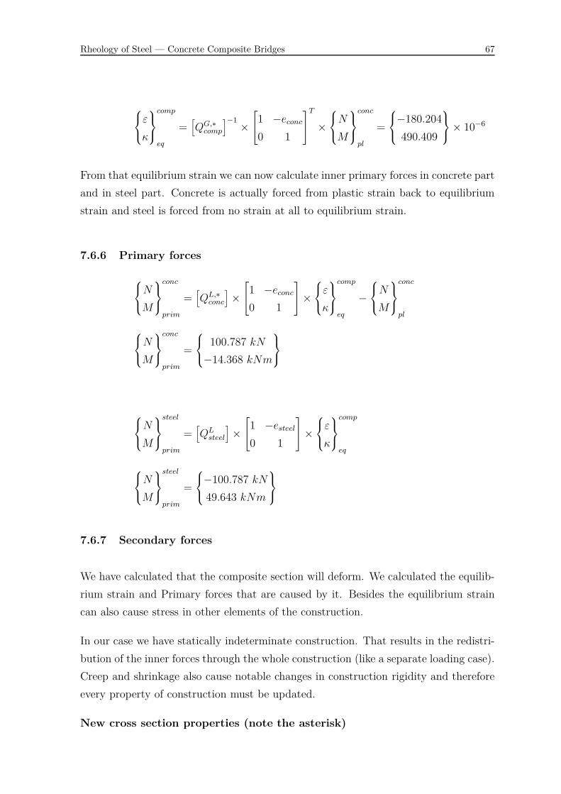
Rheology of Steel — Concrete Composite Bridges 67
⎧⎨
⎩
ε
κ
⎫⎬
⎭
comp
eq
=[
QG,∗comp]−1 ×
⎡
⎣1 −econc0 1
⎤
⎦
T
×⎧⎨
⎩
N
M
⎫⎬
⎭
conc
pl
=
⎧⎨
⎩
−180.204490.409
⎫⎬
⎭× 10−6
From that equilibrium strain we can now calculate inner primary forces in concrete partand in steel part. Concrete is actually forced from plastic strain back to equilibriumstrain and steel is forced from no strain at all to equilibrium strain.
7.6.6 Primary forces
⎧⎨
⎩
N
M
⎫⎬
⎭
conc
prim
=[
QL,∗conc]
×⎡
⎣1 −econc0 1
⎤
⎦×⎧⎨
⎩
ε
κ
⎫⎬
⎭
comp
eq
−⎧⎨
⎩
N
M
⎫⎬
⎭
conc
pl
⎧⎨
⎩
N
M
⎫⎬
⎭
conc
prim
=
⎧⎨
⎩
100.787 kN−14.368 kNm
⎫⎬
⎭
⎧⎨
⎩
N
M
⎫⎬
⎭
steel
prim
=[
QLsteel]
×⎡
⎣1 −esteel0 1
⎤
⎦×⎧⎨
⎩
ε
κ
⎫⎬
⎭
comp
eq
⎧⎨
⎩
N
M
⎫⎬
⎭
steel
prim
=
⎧⎨
⎩
−100.787 kN49.643 kNm
⎫⎬
⎭
7.6.7 Secondary forces
We have calculated that the composite section will deform. We calculated the equilib-rium strain and Primary forces that are caused by it. Besides the equilibrium straincan also cause stress in other elements of the construction.
In our case we have statically indeterminate construction. That results in the redistri-bution of the inner forces through the whole construction (like a separate loading case).Creep and shrinkage also cause notable changes in construction rigidity and thereforeevery property of construction must be updated.
New cross section properties (note the asterisk)

Rheology of Steel — Concrete Composite Bridges 68
A∗comp =Asteel × Esteel + Aconc × E∗conc
Ecomp= 397.151 cm2
e∗comp =Asteel × Esteel × Hsteel2 + Aconc ×E∗conc × (Hsteel + Hconc
2 )Asteel × Esteel + Aconc × E∗conc
e∗comp = 49.819 cm2
e∗conc = Hsteel +Hconc
2− e∗comp = 10.181 cm
e∗steel = Hsteel2− e∗comp = −24.819 cm
I∗comp =
(
Isteel + Asteel × e∗steel2)
×Esteel +(
Iconc + Aconc × e∗conc2)
× E∗concEcomp
I∗comp = 157947 cm4
Equivalent forces
Not even the centroid of cross-section is on the same position as it was before creeping.Due to that centroid movement, also the point of application for outer loading changes.To consider that change, the equilibrium strain vector must be corrected i.e. movedto new location. Movement will take place only to certain extent, in relation to howmuch the position of centroid changed:
�econc = e∗conc − econc⎧⎨
⎩
ε
κ
⎫⎬
⎭
comp,∗
eq
=
⎡
⎣1 −�econc0 1
⎤
⎦×⎧⎨
⎩
ε
κ
⎫⎬
⎭
comp
eq
Equal nodal force caused by corrected equilibrium strain is:
[
QL,∗comp]
=
⎡
⎣A∗comp ×Ecomp 0
0 I∗comp × Ecomp
⎤
⎦
⎧⎨
⎩
N
M
⎫⎬
⎭
comp
eq
=
⎡
⎣1 −e∗comp0 1
⎤
⎦×[
QL,∗comp]
×⎧⎨
⎩
ε
κ
⎫⎬
⎭
comp,∗
eq
=
⎧⎨
⎩
−1361.570 kN840.979 kNm
⎫⎬
⎭

Rheology of Steel — Concrete Composite Bridges 69
The results above suggest, that the composite girder as whole due to internal forceddeformation from creep in concrete part pulls the surrounding construction with N compeq
and bends with M compeq . To calculate how much the surrounding construction carriesthis additional loading, we must first transform finite element beam forces to finiteelement method forces, so we can obtain the loading vector for construction. Aftertransformation with respect to positive directions of degrees of freedom we obtain thecorrespondent loading vector:
{FR} =
⎧⎪⎪⎪⎪⎪⎪⎪⎪⎪⎪⎪⎪⎪⎨
⎪⎪⎪⎪⎪⎪⎪⎪⎪⎪⎪⎪⎪⎩
1361.5700
840.979−1361.570
0−840.979
⎫⎪⎪⎪⎪⎪⎪⎪⎪⎪⎪⎪⎪⎪⎬
⎪⎪⎪⎪⎪⎪⎪⎪⎪⎪⎪⎪⎪⎭
New stiffness matrix of the construction
We also have to rebuild the stiffness matrix of the system due to the change in therigidity of the structure. The stiffness matrix is assembled almost exactly as shown inthe calculation of Load case 1 only with few exceptions. Instead of properties Ecomp,Acomp, Icomp, ecomp, properties E∗comp, A∗comp, I∗comp, e∗comp is used. We will call that newreduced stiffness matrix of construction
[
KR,∗sys]
.
Movement of “free” nodes of construction due to equivalent force
{u∗} =[
KR, ∗sys
]−1 × {FR} =
⎧⎪⎪⎪⎪⎪⎪⎪⎪⎪⎪⎪⎪⎪⎨
⎪⎪⎪⎪⎪⎪⎪⎪⎪⎪⎪⎪⎪⎩
00
1.750 rad0.438 m
0−1.750 rad
⎫⎪⎪⎪⎪⎪⎪⎪⎪⎪⎪⎪⎪⎪⎬
⎪⎪⎪⎪⎪⎪⎪⎪⎪⎪⎪⎪⎪⎭
× 10−3
Strain in composite due to construction response to equivalent forces fromcreep
Equivalent force in composite is equal to:
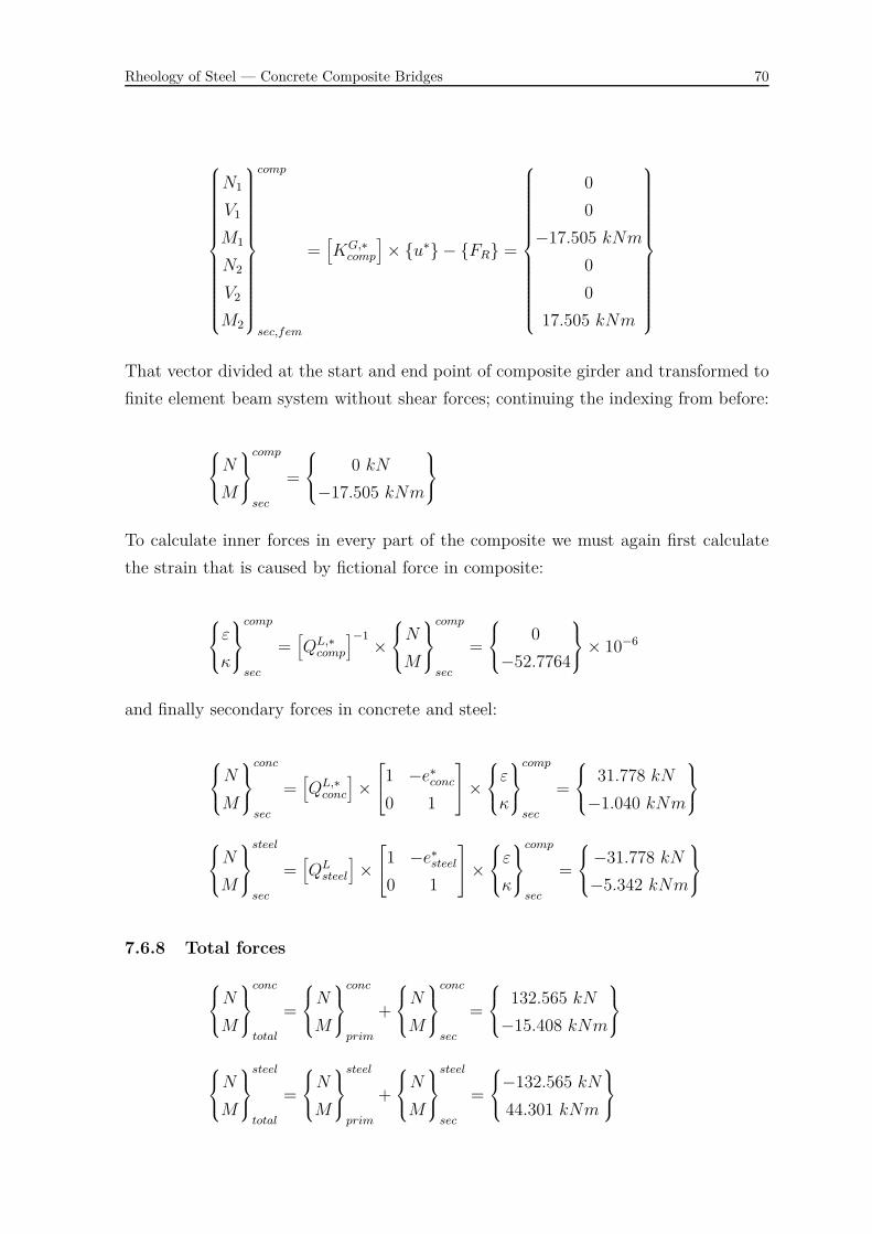
Rheology of Steel — Concrete Composite Bridges 70
⎧⎪⎪⎪⎪⎪⎪⎪⎪⎪⎪⎪⎪⎪⎨
⎪⎪⎪⎪⎪⎪⎪⎪⎪⎪⎪⎪⎪⎩
N1
V1
M1
N2
V2
M2
⎫⎪⎪⎪⎪⎪⎪⎪⎪⎪⎪⎪⎪⎪⎬
⎪⎪⎪⎪⎪⎪⎪⎪⎪⎪⎪⎪⎪⎭
comp
sec,fem
=[
KG,∗comp]
× {u∗} − {FR} =
⎧⎪⎪⎪⎪⎪⎪⎪⎪⎪⎪⎪⎪⎪⎨
⎪⎪⎪⎪⎪⎪⎪⎪⎪⎪⎪⎪⎪⎩
00
−17.505 kNm00
17.505 kNm
⎫⎪⎪⎪⎪⎪⎪⎪⎪⎪⎪⎪⎪⎪⎬
⎪⎪⎪⎪⎪⎪⎪⎪⎪⎪⎪⎪⎪⎭
That vector divided at the start and end point of composite girder and transformed tofinite element beam system without shear forces; continuing the indexing from before:
⎧⎨
⎩
N
M
⎫⎬
⎭
comp
sec
=
⎧⎨
⎩
0 kN−17.505 kNm
⎫⎬
⎭
To calculate inner forces in every part of the composite we must again first calculatethe strain that is caused by fictional force in composite:
⎧⎨
⎩
ε
κ
⎫⎬
⎭
comp
sec
=[
QL,∗comp]−1 ×
⎧⎨
⎩
N
M
⎫⎬
⎭
comp
sec
=
⎧⎨
⎩
0−52.7764
⎫⎬
⎭× 10−6
and finally secondary forces in concrete and steel:
⎧⎨
⎩
N
M
⎫⎬
⎭
conc
sec
=[
QL,∗conc]
×⎡
⎣1 −e∗conc0 1
⎤
⎦×⎧⎨
⎩
ε
κ
⎫⎬
⎭
comp
sec
=
⎧⎨
⎩
31.778 kN−1.040 kNm
⎫⎬
⎭
⎧⎨
⎩
N
M
⎫⎬
⎭
steel
sec
=[
QLsteel]
×⎡
⎣1 −e∗steel0 1
⎤
⎦×⎧⎨
⎩
ε
κ
⎫⎬
⎭
comp
sec
=
⎧⎨
⎩
−31.778 kN−5.342 kNm
⎫⎬
⎭
7.6.8 Total forces
⎧⎨
⎩
N
M
⎫⎬
⎭
conc
total
=
⎧⎨
⎩
N
M
⎫⎬
⎭
conc
prim
+
⎧⎨
⎩
N
M
⎫⎬
⎭
conc
sec
=
⎧⎨
⎩
132.565 kN−15.408 kNm
⎫⎬
⎭
⎧⎨
⎩
N
M
⎫⎬
⎭
steel
total
=
⎧⎨
⎩
N
M
⎫⎬
⎭
steel
prim
+
⎧⎨
⎩
N
M
⎫⎬
⎭
steel
sec
=
⎧⎨
⎩
−132.565 kN44.301 kNm
⎫⎬
⎭

Rheology of Steel — Concrete Composite Bridges 71
7.7 Loading case 2 – LC2: constant axial force and bendingmoment
On day 30 from casting the concrete part of the composite member we apply thesecond loading case, that is axial force on the right end of composite girder. The typeof structural system will assure that the axial force throughout the whole length of thecomposite member is constant. In addition to that, the eccentricity of applied forcealso causes constant bending moment. Loading vector with respect to reduced (or free)degrees of freedom thereby is:
{F} =
⎧⎪⎪⎪⎪⎪⎪⎪⎪⎪⎪⎪⎪⎪⎨
⎪⎪⎪⎪⎪⎪⎪⎪⎪⎪⎪⎪⎪⎩
000−1000
00
⎫⎪⎪⎪⎪⎪⎪⎪⎪⎪⎪⎪⎪⎪⎬
⎪⎪⎪⎪⎪⎪⎪⎪⎪⎪⎪⎪⎪⎭
Movement of free nodes:
{u} =[
KRsys]−1 × {F} =
⎧⎪⎪⎪⎪⎪⎪⎪⎪⎪⎪⎪⎪⎪⎨
⎪⎪⎪⎪⎪⎪⎪⎪⎪⎪⎪⎪⎪⎩
00
−5.131 rad−6.111 m
05.131 rad
⎫⎪⎪⎪⎪⎪⎪⎪⎪⎪⎪⎪⎪⎪⎬
⎪⎪⎪⎪⎪⎪⎪⎪⎪⎪⎪⎪⎪⎭
× 10−3

Rheology of Steel — Concrete Composite Bridges 72
Forces in composite:
{F compfem } =[
KLcomp]
× [Tec ]× {u} =
⎧⎪⎪⎪⎪⎪⎪⎪⎪⎪⎪⎪⎪⎪⎨
⎪⎪⎪⎪⎪⎪⎪⎪⎪⎪⎪⎪⎪⎩
1000 kN0 kN
−481.437 kNm−1000 kN
0 kN481.437 kNm
⎫⎪⎪⎪⎪⎪⎪⎪⎪⎪⎪⎪⎪⎪⎬
⎪⎪⎪⎪⎪⎪⎪⎪⎪⎪⎪⎪⎪⎭
Inner forces at left and right end of composite girder without shear forces:
⎧⎨
⎩
N
M
⎫⎬
⎭
comp
1
=
⎡
⎣1 00 −1
⎤
⎦× {F compfem }1,3 =
⎧⎨
⎩
−1000 kN−481.437 kNm
⎫⎬
⎭
⎧⎨
⎩
N
M
⎫⎬
⎭
comp
2
=
⎡
⎣1 00 −1
⎤
⎦× {F compfem }4,6 =
⎧⎨
⎩
−1000 kN−481.437 kNm
⎫⎬
⎭
As seen before, inner forces at the left and right end of composite girder are symmet-rical. As already seen at the same place in LC1, from here on only simpler notationsof N and M will be used. The same is valid for similar symbols.
[
QLcomp]
=
⎡
⎣Acomp × Ecomp 0
0 Icomp ×Ecomp
⎤
⎦
[
QLcomp]
=
⎡
⎣12626130 kN 0
0 375321 kNm2
⎤
⎦
Deformations in composite due LC2:
⎧⎨
⎩
ε
κ
⎫⎬
⎭
comp
=[
QLcomp]−1 ×
⎧⎨
⎩
N
M
⎫⎬
⎭
comp
=
⎧⎨
⎩
−79.201−1282.730
⎫⎬
⎭× 10−6

Rheology of Steel — Concrete Composite Bridges 73
7.7.1 Primary forces
⎧⎨
⎩
N
M
⎫⎬
⎭
conc
prim
=
⎧⎨
⎩
N
M
⎫⎬
⎭
steel
prim
=
⎧⎨
⎩
0 kN0 kNm
⎫⎬
⎭
7.7.2 Secondary forces
Forces in concrete part of the composite girder
Elasticity matrix of concrete part of composite – Qconc,
[
QLconc]
=
⎡
⎣Aconc × Econc 0
0 Iconc × Econc
⎤
⎦ =
⎡
⎣10200000 kN 0
0 34000 kNm2
⎤
⎦
transformation of deformation from local composite coordinate system to local concretecoordinate system.
⎧⎨
⎩
ε
κ
⎫⎬
⎭
conc
=
⎡
⎣1 −econc0 1
⎤
⎦×⎧⎨
⎩
ε
κ
⎫⎬
⎭
comp
=
⎡
⎣7.067−1282.730
⎤
⎦× 10−6
and finally secondary forces in concrete part.
⎧⎨
⎩
N
M
⎫⎬
⎭
conc
sec
= [Qconc]×⎧⎨
⎩
ε
κ
⎫⎬
⎭
conc
=
⎧⎨
⎩
72.082 kN−43.613 kNm
⎫⎬
⎭
Secondary forces in steel part of the composite girder
Elasticity matrix of steel part of composite – Qsteel,
[
QLsteel]
=
⎡
⎣Asteel ×Esteel 0
0 Isteel × Esteel
⎤
⎦ =
⎡
⎣10200000 kN 0
0 34000 kNm2
⎤
⎦
transformation of deformation from local composite coordinate system to local steelcoordinate system.

Rheology of Steel — Concrete Composite Bridges 74
⎧⎨
⎩
ε
κ
⎫⎬
⎭
steel
=
⎡
⎣1 −esteel0 1
⎤
⎦×⎧⎨
⎩
ε
κ
⎫⎬
⎭
comp
=
⎡
⎣−441.890−1282.730
⎤
⎦× 10−6
and finally secondary forces in steel part.
⎧⎨
⎩
N
M
⎫⎬
⎭
steel
sec
=[
QLsteel]
×⎧⎨
⎩
ε
κ
⎫⎬
⎭
steel
=
⎧⎨
⎩
−1072.080 kN−129.849 kNm
⎫⎬
⎭
7.7.3 Total forces
⎧⎨
⎩
N
M
⎫⎬
⎭
conc
total
=
⎧⎨
⎩
N
M
⎫⎬
⎭
conc
prim
+
⎧⎨
⎩
N
M
⎫⎬
⎭
conc
sec
=
⎧⎨
⎩
72.082 kN−43.613 kNm
⎫⎬
⎭
⎧⎨
⎩
N
M
⎫⎬
⎭
steel
total
=
⎧⎨
⎩
N
M
⎫⎬
⎭
steel
prim
+
⎧⎨
⎩
N
M
⎫⎬
⎭
steel
sec
=
⎧⎨
⎩
−1072.080 kN−129.849 kNm
⎫⎬
⎭

Rheology of Steel — Concrete Composite Bridges 75
7.8 Creep & Shrinkage 2 – CRSH2: day 30 — 10000
7.8.1 Creep coefficients for loading cases
t1 = 30 days
t2 = 10000 days
tLC1 = 10 days
ΦLC1 = φ(10000, 10)− φ(30, 10) = 1.895
ΦCRSH1 = φ(10000, 20)− φ(30, 20) = 1.826
ΦLC2 = φ(10000, 30)− φ(30, 30) = 2.362
7.8.2 Elastic deformations
⎧⎨
⎩
ε
κ
⎫⎬
⎭
conc
LC1,el
=[
QLconc]−1 ×
⎧⎨
⎩
N
M
⎫⎬
⎭
conc
total
=
⎧⎨
⎩
−80.0961200.389
⎫⎬
⎭× 10−6
⎧⎨
⎩
ε
κ
⎫⎬
⎭
conc
CRSH1,el
=[
QLconc]−1 ×
⎧⎨
⎩
N
M
⎫⎬
⎭
conc
total
=
⎧⎨
⎩
12.996−453.187
⎫⎬
⎭× 10−6
⎧⎨
⎩
ε
κ
⎫⎬
⎭
conc
LC2,el
=[
QLconc]−1 ×
⎧⎨
⎩
N
M
⎫⎬
⎭
conc
total
=
⎧⎨
⎩
7.067−128.273
⎫⎬
⎭× 10−6

Rheology of Steel — Concrete Composite Bridges 76
7.8.3 Shrinkage strain
10 50 100 500 1000 5000 1 � 104�0.0007
�0.0006
�0.0005
�0.0004
�0.0003
�0.0002
�0.0001
0.0000
time �days�
shri
nkag
est
rain
�� c
s
Figure 27: concrete shrinkage with time
εcs,CRSH2 = εcs(t2, ts)− εcs(t1, ts)
εcs,CRSH2 = εcs(10000, 10)− εcs(30, 10)
εcs,CRSH2 =
⎧⎨
⎩
−442.7390
⎫⎬
⎭× 10−6

Rheology of Steel — Concrete Composite Bridges 77
7.8.4 Plastic deformation
⎧⎨
⎩
ε
κ
⎫⎬
⎭
conc
pl
=n∑
i=1Φn ×
⎧⎨
⎩
ε
κ
⎫⎬
⎭
conc
n,el
+ εcs
⎧⎨
⎩
ε
κ
⎫⎬
⎭
conc
pl
= ΦLC1 ×⎧⎨
⎩
ε
κ
⎫⎬
⎭
conc
LC1,el
+ ΦCRSH1 ×⎧⎨
⎩
ε
κ
⎫⎬
⎭
conc
CRSH1,el
+ ΦLC2 ×⎧⎨
⎩
ε
κ
⎫⎬
⎭
conc
LC2,el
+ εcs,CRSH1
⎧⎨
⎩
ε
κ
⎫⎬
⎭
conc
pl
=
⎧⎨
⎩
−555.75−1575.75
⎫⎬
⎭× 10−6

Rheology of Steel — Concrete Composite Bridges 78
7.8.5 Equilibrium strain
tW = 0.5× t1 + 0.5× t2 = 0.5× 30 + 0.5× 10000 = 4985 days
ΦW = φ (10000, 4985)− φ (4985, 4985) = 0.859
E∗conc =1
1 + ΦWEconc = 1.829× 10⁷kN
m2
�W�LC1 �CRSH1 �LC2
10 50 100 500 1000 5000 1 � 1040.0
0.5
1.0
1.5
2.0
2.5
3.0
3.5
time �days�
cree
pfa
ctor
�Φ�
t,t 0�
Figure 28: From left to right: Creep curve for LC1 (solid line), CRSH1 (dashedline), LC2 (solid line), CRSH2 – ΦW (dashed line)
[
QL,∗conc]
= 11 + ΦW
×⎡
⎣Aconc × Econc 0
0 Iconc ×Econc
⎤
⎦
[
QL,∗conc]
=
⎡
⎣5486980 kN 0
0 18289.9 kNm2
⎤
⎦
⎧⎨
⎩
N
M
⎫⎬
⎭
conc
pl
=[
QL,∗conc]
×⎧⎨
⎩
ε
κ
⎫⎬
⎭
conc
pl
=
⎧⎨
⎩
−3049.390 kN−28.820 kNm
⎫⎬
⎭

Rheology of Steel — Concrete Composite Bridges 79
[
QG,∗comp]
=
⎡
⎣1 −econc0 1
⎤
⎦
T
×[
QL,∗conc]
×⎡
⎣1 −econc0 1
⎤
⎦
+
⎡
⎣1 −esteel0 1
⎤
⎦
T
×[
QL,∗steel]
×⎡
⎣1 −esteel0 1
⎤
⎦
[
QG,∗comp]
=
⎡
⎣7913110 kN 316965 kNm316965 kNm 338295 kNm2
⎤
⎦
⎧⎨
⎩
ε
κ
⎫⎬
⎭
comp
eq
=[
QG,∗comp]−1 ×
⎡
⎣1 −econc0 1
⎤
⎦
T
×⎧⎨
⎩
N
M
⎫⎬
⎭
conc
pl
=
⎧⎨
⎩
−422.069916.483
⎫⎬
⎭× 10−6
7.8.6 Primary forces
⎧⎨
⎩
N
M
⎫⎬
⎭
conc
prim
=[
QL,∗conc]
×⎡
⎣1 −econc0 1
⎤
⎦×⎧⎨
⎩
ε
κ
⎫⎬
⎭
comp
eq
−⎧⎨
⎩
N
M
⎫⎬
⎭
conc
pl
⎧⎨
⎩
N
M
⎫⎬
⎭
conc
prim
=
⎧⎨
⎩
395.305 kN45.583 kNm
⎫⎬
⎭
⎧⎨
⎩
N
M
⎫⎬
⎭
steel
prim
=[
QLsteel]
×⎡
⎣1 −esteel0 1
⎤
⎦×⎧⎨
⎩
ε
κ
⎫⎬
⎭
comp
eq
⎧⎨
⎩
N
M
⎫⎬
⎭
steel
prim
=
⎧⎨
⎩
−395.305 kN92.774 kNm
⎫⎬
⎭
7.8.7 Secondary forces
New cross section properties
A∗comp = Asteel × Esteel + Aconc × E∗conc
Ecomp= 376.815 cm2

Rheology of Steel — Concrete Composite Bridges 80
e∗comp =Asteel × Esteel × Hsteel2 + Aconc ×E∗conc × (Hsteel + Hconc
2 )Asteel × Esteel + Aconc × E∗conc
e∗comp = 49.269 cm2
e∗conc = Hsteel +Hconc
2− e∗comp = 10.73110.181 cm
e∗steel = Hsteel2− e∗comp = −24.269 cm
I∗comp =
(
Isteel + Asteel × e∗steel2)
×Esteel +(
Iconc + Aconc × e∗conc2)
× E∗concEcomp
I∗comp = 155047 cm4
Equivalent forces�econc = e∗conc − econc
⎧⎨
⎩
ε
κ
⎫⎬
⎭
comp,∗
eq
=
⎡
⎣1 −�econc0 1
⎤
⎦×⎧⎨
⎩
ε
κ
⎫⎬
⎭
comp
eq
[
QL,∗comp]
=
⎡
⎣A∗comp ×Ecomp 0
0 I∗comp × Ecomp
⎤
⎦
⎧⎨
⎩
N
M
⎫⎬
⎭
comp
eq
=
⎡
⎣1 −e∗comp0 1
⎤
⎦×[
QL,∗comp]
×⎧⎨
⎩
ε
κ
⎫⎬
⎭
comp,∗
eq
=
⎧⎨
⎩
−3049.390 kN1800.810 kNm
⎫⎬
⎭
{FR} =
⎧⎪⎪⎪⎪⎪⎪⎪⎪⎪⎪⎪⎪⎪⎨
⎪⎪⎪⎪⎪⎪⎪⎪⎪⎪⎪⎪⎪⎩
3049.3900
1800.810−3049.390
0−1800.810
⎫⎪⎪⎪⎪⎪⎪⎪⎪⎪⎪⎪⎪⎪⎬
⎪⎪⎪⎪⎪⎪⎪⎪⎪⎪⎪⎪⎪⎭
New stiffness matrix of the construction
Exactly as in CRSH1 the stiffness or rigidity of construction must be updated accord-ingly. For further detail see the same section of CRSH1.
Movement of “free” nodes of construction due equivalent force

Rheology of Steel — Concrete Composite Bridges 81
{u} =[
KR, ∗sys
]−1 × {FR} =
⎧⎪⎪⎪⎪⎪⎪⎪⎪⎪⎪⎪⎪⎪⎨
⎪⎪⎪⎪⎪⎪⎪⎪⎪⎪⎪⎪⎪⎩
00
3.265 rad0.134 m
0−3.265 rad
⎫⎪⎪⎪⎪⎪⎪⎪⎪⎪⎪⎪⎪⎪⎬
⎪⎪⎪⎪⎪⎪⎪⎪⎪⎪⎪⎪⎪⎭
× 10−3

Rheology of Steel — Concrete Composite Bridges 82
Strain in composite due construction response to equivalent forces fromcreep
⎧⎪⎪⎪⎪⎪⎪⎪⎪⎪⎪⎪⎪⎪⎨
⎪⎪⎪⎪⎪⎪⎪⎪⎪⎪⎪⎪⎪⎩
N1
V1
M1
N2
V2
M2
⎫⎪⎪⎪⎪⎪⎪⎪⎪⎪⎪⎪⎪⎪⎬
⎪⎪⎪⎪⎪⎪⎪⎪⎪⎪⎪⎪⎪⎭
comp
sec,fem
=[
KG,∗comp]
× {u} − {FR} =
⎧⎪⎪⎪⎪⎪⎪⎪⎪⎪⎪⎪⎪⎪⎨
⎪⎪⎪⎪⎪⎪⎪⎪⎪⎪⎪⎪⎪⎩
00
−32.648 kNm00
32.648 kNm
⎫⎪⎪⎪⎪⎪⎪⎪⎪⎪⎪⎪⎪⎪⎬
⎪⎪⎪⎪⎪⎪⎪⎪⎪⎪⎪⎪⎪⎭
⎧⎨
⎩
N
M
⎫⎬
⎭
comp
sec
=
⎧⎨
⎩
0 kN−16, 988 kNm
⎫⎬
⎭
⎧⎨
⎩
ε
κ
⎫⎬
⎭
comp
sec
=[
QL,∗comp]−1 ×
⎧⎨
⎩
N
M
⎫⎬
⎭
comp
sec
=
⎧⎨
⎩
0−100.272
⎫⎬
⎭× 10−6
⎧⎨
⎩
N
M
⎫⎬
⎭
conc
sec
=[
QL,∗conc]
×⎡
⎣1 −e∗conc0 1
⎤
⎦×⎧⎨
⎩
ε
κ
⎫⎬
⎭
comp
sec
=
⎧⎨
⎩
59.040 kN−1.834 kNm
⎫⎬
⎭
⎧⎨
⎩
N
M
⎫⎬
⎭
steel
sec
=[
QLsteel]
×⎡
⎣1 −e∗steel0 1
⎤
⎦×⎧⎨
⎩
ε
κ
⎫⎬
⎭
comp
sec
=
⎧⎨
⎩
−59.040 kN−10.150 kNm
⎫⎬
⎭
7.8.8 Total forces
⎧⎨
⎩
N
M
⎫⎬
⎭
conc
total
=
⎧⎨
⎩
N
M
⎫⎬
⎭
conc
prim
+
⎧⎨
⎩
N
M
⎫⎬
⎭
conc
sec
=
⎧⎨
⎩
454.346 kN43.749 kNm
⎫⎬
⎭
⎧⎨
⎩
N
M
⎫⎬
⎭
steel
total
=
⎧⎨
⎩
N
M
⎫⎬
⎭
steel
prim
+
⎧⎨
⎩
N
M
⎫⎬
⎭
steel
sec
=
⎧⎨
⎩
−454.346 kN82.624 kNm
⎫⎬
⎭

Rheology of Steel — Concrete Composite Bridges 83
7.9 Summary
In this simple example we could see the influence of creep and shrinkage in concrete onthe whole composite construction. The methodology of calculating creep and shrinkagewas shown. Even though we only used one time step per interval to calculate them,the solution is fairly accurate and user frendly to calculate manually.
Numerical results for this example are presented in the table on the following page. Aseach loading case’s total forces represent only a stress/force increment, the real amountof stress/force per material can be calculated only by summing-up loading case resultswhich occured up to the observed day in structural analysis.

Rheology
ofSteel—C
oncreteC
omposite
Bridges
84
Time Loading case
Total inner forcesTotal inner forces increments Total inner forces increments sum
Concrete Steel Concrete SteelN [kN] M [kNm] N [kN] M [kNm] N [kN] M [kNm] N [kN] M [kNm]
10 LC1: constant bending moment -825.843 40.932 825.843 121.867 -825.843 40.932 825.843 121.86710 — 30 CRSH1: creep and shrinkage 132.565 -15.408 -132.565 44.301 -693.278 25.524 692.435 166.168
30 LC2: constant axial force and bending moment 72.082 -43.613 -1072.080 -129.849 -621.196 -18.089 -379.645 36.31930 — 10000 CRSH2: creep and shrinkage 454.346 43.749 -454.346 82.624 -166.850 25.660 -833.961 118.943
Table 2: Results of structural analysis per loading case and stress history

Rheology of Steel — Concrete Composite Bridges 85
7.10 Calculation of example 1 with RM Bridge
7.10.1 Material data
Figure 29: Material properties of steel

Rheology of Steel — Concrete Composite Bridges 86
Figure 30: Material properties of concrete
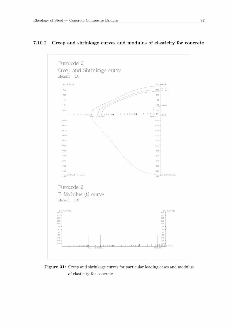
Rheology of Steel — Concrete Composite Bridges 87
7.10.2 Creep and shrinkage curves and modulus of elasticity for concrete
Figure 31: Creep and shrinkage curves for particular loading cases and modulusof elasticity for concrete

Rheology of Steel — Concrete Composite Bridges 88
7.10.3 Cross — section properties
Figure 32: Cross — section properties for steel part of composite

Rheology of Steel — Concrete Composite Bridges 89
Figure 33: Cross — section properties for concrete part of composite

Rheology of Steel — Concrete Composite Bridges 90
Figure 34: Cross — section properties for whole composite

Rheology of Steel — Concrete Composite Bridges 91
7.10.4 Results — comparison with and without reology effects
Figure 35: Axial force in steel
Figure 36: Axial force in concrete

Rheology of Steel — Concrete Composite Bridges 92
Figure 37: Bending moment in steel
Figure 38: Bending moment in concrete

Rheology of Steel — Concrete Composite Bridges 93
8 Example 2 — composite 3 span bridge

Rheology of Steel — Concrete Composite Bridges 94
8.1 Introduction
In this example we will make a structural analysis of a three span steel – concretecomposite bridge as can be found in practice. Bridge is stressed only with the selfweight of built-in materials. Structural analysis will be made per construction stageand with consideration of creep and shrinkage effects of concrete. For this calculationand presentation of results software RM Bridge is used.
This bridge’s deck is composed (as seen in Figure 39) of steel hollow box and a concreteslab above it. Above the piers the steel box is stronger due to greater supporting forceand bending moment. Material used for steel hollow box is S355. Material for the twopiers is concrete of quality C30/37 and for the top concrete deck of the bridge C45/55.
The whole bridge is built in 4 stages and time dependent effects of concrete betweenthese stages are considered. In the first construction stage the two supporting piersare build and after 42 days steel hollow-box is set in place. In the second constructionstage the top slab of the bridge with exceptions over the piers is concreted. After that,the 14 day creep and shrinkage interval begins. After that time, the remaining gapsin concrete bridge deck are concreted and additional dead load such as pavement andpublic lighting is superimposed. In continuation follows the creep and shrinkage intervalup to day 10000 which corresponds the theoretical lifetime of the whole construction.
Results of structural analyses will be presented in two different ways: incrementaland summarized. Incremental results represent inner statical forces due to particularloading case calculated at that time. The sum results represent the sum of incrementalinner statical forces due to all loading cases that occur up to this calculation time. Thelast loading case’s sum results represent the final stage of inner statical forces at day10000.

Rheology of Steel — Concrete Composite Bridges 95
8.2 Cross — section properties
Figure 39: Cross — section properties for steel part of composite main girderin spans
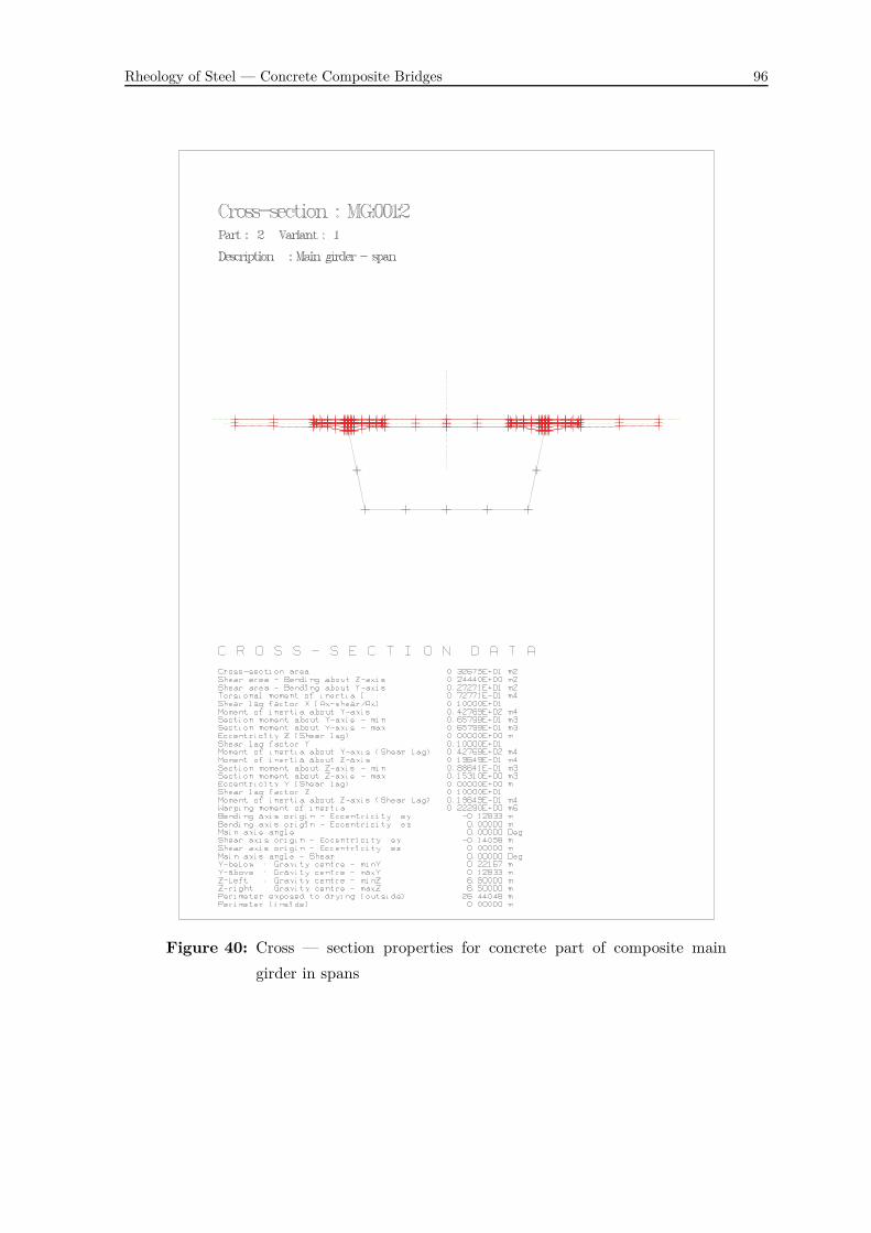
Rheology of Steel — Concrete Composite Bridges 96
Figure 40: Cross — section properties for concrete part of composite maingirder in spans

Rheology of Steel — Concrete Composite Bridges 97
Figure 41: Cross — section properties for composite main girder (equivalentcomposite cross — section) in spans

Rheology of Steel — Concrete Composite Bridges 98
Figure 42: Cross — section properties for steel part of composite main girdernear abutments

Rheology of Steel — Concrete Composite Bridges 99
Figure 43: Cross — section properties for concrete part of composite maingirder near abutments

Rheology of Steel — Concrete Composite Bridges 100
Figure 44: Cross — section properties for composite main girder (equivalentcomposite cross — section) near abutments

Rheology of Steel — Concrete Composite Bridges 101
Figure 45: Cross — section properties for piers

Rheology of Steel — Concrete Composite Bridges 102
8.3 Results
8.3.1 LC1: Self weight of steel girders

Rheology of Steel — Concrete Composite Bridges 103
8.3.2 LC2: Self weight of concrete slab at span middle

Rheology of Steel — Concrete Composite Bridges 104
8.3.3 LC3: Self weight of concrete slab above piers

Rheology of Steel — Concrete Composite Bridges 105
8.3.4 CRSH1: Creep and shrinkage of concrete for 14 days

Rheology of Steel — Concrete Composite Bridges 106
8.3.5 LC4: Superimposed dead load

Rheology of Steel — Concrete Composite Bridges 107
8.3.6 CRSH2: Creep and shrinkage of concrete up to day 10000

Rheology of Steel — Concrete Composite Bridges 108
9 Conclusion
In this work we examined the influence of time dependent material properties of con-crete as part of steel – concrete composite construction. We introduced the timedependent effects of concrete and design models describing their behaviour. Basedon the CEB–FIP 1990 Model Code the methodology of numerical creep and shrink-age prediction was introduced and first one simple example with detailed descriptionsolved. However, the main purpouse of the given example was only to demonstate thenumerical approach of structural analysis with time effects considered. The loadingcases used in that example do not match the real common bridge constructions.
For that reason one more advanced and more realistic example was calculated usingsoftware package RM Bridge. This software package does not employ the same an-alytical approach that we used in our first example, but it produces similar results.Where we used the method with age-adjusted modulus of elasticity, RM Bridge usedan internal iterative algorithm based on Newton–Raphson procedure.
For purpose of simplicity in example 1, only one time step for the whole intervalof final creep calculation was used. In the second example, where we used only thesoftware package RM Bridge, for the final creep interval, three time steps were used withlogarithmic division. Results gained from that structural analysis showed that the axialforce in concrete deck in the middle of the composite bridge main span changed dueto creep and shrinkage in concrete from –4132 kN (compression) to 1240 kN (tension),which appears mainly due to shrinkage, making concrete in construction working fromfavourable to un-favourable. When concrete relaxes due to creep and shrinks, addingaditional tension to construction, stress on steel increases. Bending moment in steel inthe middle of the main span increased from 17613 kNm to 18238 kNm which representsexactly 3.5 % change. Even with concrete working from favourable to un-favourable thevertical deformation in the middle of the main span gained only 10 mm, by increasingfrom 166 mm to 176 mm, representing a 6 % change.
The conclusion of this work is that time dependent material properties of concretecan cause significant changes in the inner forces of construction. When structuralyanalysing steel — concrete composite bridges, time dependant effects of concrete mustalways be considered.

Rheology of Steel — Concrete Composite Bridges 109
References
[1] RM Bridge Reference Manual. Bentley Systems, Incorporated, Exton, 2008.
[2] David Collings. Steel-concrete Composite Bridges. Thomas Telford, London, 2005.
[3] Comité Euro-International du Béton as Bulletins d’Information. CEB-FIPMODEL CODE 1990. Thomas Telford, London, 1993.
[4] Amin Ghali, Renaud Favre, and M. Elbadry. Concrete Structures: Stresses andDeformations. Taylor and Francis, edition: 3, illustrated edition, 2002.
[5] C. R. Hendy and R. P. Johnson. Designers’ Guide to EN 1994-2: Design ofComposite Steel and Concrete Structures Part 2, General Rules and Rules forBridges. Thomas Telford, London, 2006.
[6] Dorian Janjic and Martin Pircher. Long term effects & specific prob-lems in concrete & composite bridges. preprint (2004), available athttp://www.tdv0.com/staticstate/softfile/20070322/TY-usC7YWJs6F.pdf.
[7] Boris Lutar and Janez Duhovnik. Metoda končnih elementov za linijske konstruk-cije. Fakulteta za Gradbeništvo, Maribor, 2004.
[8] Edward G. Nawy. Concrete Construction Engineering Handbook. CRC Press,London, edition: 2, illustrated, revised edition, 2008.
[9] M. J. Ryall, G. A. R. Parke, J. E. Harding, Institution of Civil Engineers, andInstitution of Civil Engineers (Great Britain). The Manual of Bridge Engineering.Thomas Telford, London, 2000.
[10] Miodrag Sekulović. Metod konačnih elemenata. Građevinska knjiga, Beograd,1984.