University of Groningen Accelerating Wavelet Lifting on ... Wavelet Lifting on Graphics Hardware Using CUDA Wladimir J. van der Laan, Andrei C. Jalba, and Jos B.T.M. Roerdink,Senior

University of Groningen

Accelerating Wavelet Lifting on Graphics Hardware Using CUDALaan, Wladimir J. van der; Jalba, Andrei C.; Roerdink, Johannes

Published in:Ieee transactions on parallel and distributed systems

DOI:10.1109/TPDS.2010.143

IMPORTANT NOTE: You are advised to consult the publisher's version (publisher's PDF) if you wish to cite fromit. Please check the document version below.

Document VersionPublisher's PDF, also known as Version of record

Publication date:2011

Link to publication in University of Groningen/UMCG research database

Citation for published version (APA):Laan, W. J. V. D., Jalba, A. C., & Roerdink, J. B. T. M. (2011). Accelerating Wavelet Lifting on GraphicsHardware Using CUDA. Ieee transactions on parallel and distributed systems, 22(1), 132-146. DOI:10.1109/TPDS.2010.143

CopyrightOther than for strictly personal use, it is not permitted to download or to forward/distribute the text or part of it without the consent of theauthor(s) and/or copyright holder(s), unless the work is under an open content license (like Creative Commons).

Take-down policyIf you believe that this document breaches copyright please contact us providing details, and we will remove access to the work immediatelyand investigate your claim.

Downloaded from the University of Groningen/UMCG research database (Pure): http://www.rug.nl/research/portal. For technical reasons thenumber of authors shown on this cover page is limited to 10 maximum.

Download date: 25-06-2018

https://doi.org/10.1109/TPDS.2010.143

https://www.rug.nl/research/portal/en/publications/accelerating-wavelet-lifting-on-graphics-hardware-using-cuda(4acd6338-397d-4f48-a0d3-e58cdbc7d45f).html

Accelerating Wavelet Lifting on GraphicsHardware Using CUDA

Wladimir J. van der Laan, Andrei C. Jalba, and Jos B.T.M. Roerdink, Senior Member, IEEE

Abstract—The Discrete Wavelet Transform (DWT) has a wide range of applications from signal processing to video and image

compression. We show that this transform, by means of the lifting scheme, can be performed in a memory and computation-efficient way

on modern, programmable GPUs, which can be regarded as massively parallel coprocessors through NVidia’s CUDA compute

paradigm. The three main hardware architectures for the 2D DWT (row-column, line-based, block-based) are shown to be unsuitable for

a CUDA implementation. Our CUDA-specific design can be regarded as a hybrid method between the row-column and block-based

methods. We achieve considerable speedups compared to an optimized CPU implementation and earlier non-CUDA-based GPU DWT

methods, both for 2D images and 3D volume data. Additionally, memory usage can be reduced significantly compared to previous GPU

DWT methods. The method is scalable and the fastest GPU implementation among the methods considered. A performance analysis

shows that the results of our CUDA-specific design are in close agreement with our theoretical complexity analysis.

Index Terms—Discrete wavelet transform, wavelet lifting, graphics hardware, CUDA.

Ç

1 INTRODUCTION

THE wavelet transform, originally developed as a tool forthe analysis of seismic data, has been applied in areas as

diverse as signal processing, video and image coding,compression, data mining, and seismic analysis. The theoryof wavelets bears a large similarity to Fourier analysis, wherea signal is approximated by superposition of sinusoidalfunctions. A problem, however, is that the sinusoids have aninfinite support, which makes Fourier analysis less suitableto approximate sharp transitions in the function or signal.Wavelet analysis overcomes this problem by using smallwaves, called wavelets, which have a compact support. Onestarts with a wavelet prototype function, called a basic waveletor mother wavelet. Then, a wavelet basis is constructed bytranslated and dilated (i.e., rescaled) versions of the basicwavelet. The fundamental idea is to decompose a signal intocomponents with respect to this wavelet basis, and toreconstruct the original signal as a superposition of waveletbasis functions; therefore, we speak a multiresolution analysis.If the shape of the wavelets resembles that of the data, thewavelet analysis results in a sparse representation of thesignal, making wavelets an interesting tool for datacompression. This also allows a client-server model of dataexchange, where data are first decomposed into differentlevels of resolution on the server, then progressivelytransmitted to the client, where the data can be incrementallyrestored as it arrives (“progressive refinement”). This is

especially useful when the data sets are very large, as in thecase of 3D data visualization [1]. For some general back-ground on wavelets, the reader is referred to the books byDaubechies [2] or Mallat [3].

In the theory of wavelet analysis, both continuous anddiscrete wavelet transforms are defined. If discrete andfinite data are used, it is appropriate to consider the DiscreteWavelet Transform (DWT). Like the discrete Fourier trans-form (DFT), the DWT is a linear and invertible transformthat operates on a data vector whose length is (usually) aninteger power of 2. The elements of the transformed vectorare called wavelet coefficients, in analogy of Fourier coeffi-cients in case of the DFT. The DWT and its inverse can becomputed by an efficient filter bank algorithm, calledMallat’s pyramid algorithm [3]. This algorithm involvesrepeated downsampling (forward transform) or upsam-pling (inverse transform) and convolution filtering by theapplication of high and low-pass filters. Its complexity islinear in the number of data elements.

In the construction of so-called first-generation waveletbases, which are translates and dilates of a single basicfunction, Fourier transform techniques played a major role[2]. To deal with situations where the Fourier transform isnot applicable, such as wavelets on curves or surfaces, orwavelets for irregularly sampled data, second-generationwavelets were proposed by Sweldens, based on the so-called lifting scheme [4]. This provides a flexible andefficient framework for building wavelets. It works entirelyin the original time/space domain and does not involveFourier transforms.

The basic idea behind the lifting scheme is as follows: Itstarts with a simple wavelet, and then, gradually builds anew wavelet, with improved properties, by adding newbasis functions. So, the simple wavelet is lifted to a newwavelet, and this can be done repeatedly. Alternatively, onecan say that a complex wavelet transform is factored into asequence of simple lifting steps [5]. More details on liftingare provided in Section 3.

132 IEEE TRANSACTIONS ON PARALLEL AND DISTRIBUTED SYSTEMS, VOL. 22, NO. 1, JANUARY 2011

. W.J. van der Laan and J.B.T.M. Roerdink are with the Johann BernoulliInstitute for Mathematics and Computer Science, University of Groningen,PO Box 407, 9700 AK Groningen, The Netherlands.E-mail: [email protected], [email protected].

. A.C. Jalba is with the Institute for Mathematics and Computing Science,Eindhoven University of Technology, PO Box 513, 5600 MB Eindhoven,The Netherlands. E-mail: [email protected].

Manuscript received 4 Sept. 2009; revised 23 Feb. 2010; accepted 2 June 2010;published online 28 July 2010.Recommended for acceptance by D.A. Bader, D. Kaeli, and V. Kindratenko.For information on obtaining reprints of this article, please send e-mail to:[email protected], and reference IEEECS Log Number TPDS-2009-09-0403.Digital Object Identifier no. 10.1109/TPDS.2010.143.

1045-9219/11/$26.00 � 2011 IEEE Published by the IEEE Computer Society

Also, for first-generation wavelets, constructing them bythe lifting scheme has a number of advantages [4]. First, itresults in a faster implementation of the wavelet transformthan the straightforward convolution-based approach byreducing the number of arithmetic operations. Asymptoti-cally, for long filters, lifting is twice as fast as the standardalgorithm. Second, given the forward transform, the inversetransform can be found in a trivial way. Third, no Fouriertransforms are needed. Lastly, it allows a fully in-placecalculation of the wavelet transform, so no auxiliarymemory is needed. With the generally limited amount ofhigh-speed memory available, and the large quantities ofdata that have to be processed in multimedia or visualiza-tion applications, this is a great advantage. Finally, thelifting scheme represents a universal discrete wavelettransform which involves only integer coefficients insteadof the usual floating point coefficients [6]. Therefore, webased our DWT implementation on the lifting scheme.

Custom hardware implementations of the DWT havebeen developed to meet the computational demands forsystems that handle the enormous throughputs in, forexample, real-time multimedia processing. However, costand availability concerns and the inherent inflexibility ofthis kind of solutions make it preferable to use a morewidespread and general platform. NVidia’s G80 architec-ture [7], introduced in 2006 with the GeForce 8800 GPU,provides such a platform. It is a highly parallel computingarchitecture available for systems ranging from laptops ordesktop computers to high-end compute servers. In thispaper, we will present a hardware-accelerated DWTalgorithm that makes use of the Compute Unified DeviceArchitecture (CUDA) parallel programming model to fullyexploit the new features offered by the G80 architecturewhen compared to traditional GPU programming.

The three main hardware architectures for the 2D DWT,i.e., row-column, line-based, or block-based, turn out to beunsuitable for a CUDA implementation (see Section 2). Thebiggest challenge of fitting wavelet lifting in the SIMDmodel is that data sharing is, in principle, needed afterevery lifting step. This makes the division into independentcomputational blocks difficult, and means that a compro-mise has to be made between minimizing the amount ofdata shared with neighboring blocks (implying moresynchronization overhead) and allowing larger data overlapin the computation at the borders (more computationoverhead). This challenge is specifically difficult withCUDA, as blocks cannot exchange data at all withoutreturning execution flow to the CPU. Our solution is asliding window approach which enables us (in the case ofseparable wavelets) to keep intermediate results longer inshared memory, instead of being written to global memory.Our CUDA-specific design can be regarded as a hybridmethod between the row-column and block-based methods.We implemented our methods both for 2D and 3D data, andobtained considerable speedups compared to an optimizedCPU implementation and earlier non-CUDA-based GPUDWT methods. Additionally, memory usage can be reducedsignificantly compared to previous GPU DWT methods.The method is scalable and the fastest GPU implementationamong the methods considered. A performance analysisshows that the results of our CUDA-specific design are inclose agreement with our theoretical complexity analysis.

The paper is organized as follows: Section 2 gives a briefoverview of GPU wavelet lifting methods, and previouswork on GPU wavelet transforms. In Section 3, we presentthe basic theory of wavelet lifting. Section 4 first presents anoverview of the CUDA programming environment andexecution model, introduces some performance considera-tions for parallel CUDA programs, and gives the details ofour wavelet lifting implementation on GPU hardware.Section 5 presents benchmark results and analyzes theperformance of our method. Finally, in Section 6, we drawconclusions and discuss future avenues of research.

2 PREVIOUS AND RELATED WORK

In [8], a method was first proposed that makes use ofOpenGL extensions on early nonprogrammable graphicshardware to perform the convolution and downsampling/upsampling for a 2D DWT. Later, in [9], this was general-ized to 3D using a technique called tile boarding.

Wong et al. [10] implemented the DWT on program-mable graphics hardware with the goal of speeding upJPEG2000 compression. They made the decision not to usewavelet lifting, based on the rationale that, although liftingrequires less memory and less computations, it imposes anorder of execution which is not fully parallelizable. Theyassumed that lifting would require more rendering passes,and therefore, in the end be slower than the standardapproach based on convolution.

However, Tenllado et al. [11] performed wavelet liftingon conventional graphics hardware by splitting the compu-tation into four passes using fragment shaders. Theyconcluded that a gain of 10-20 percent could be obtainedby using lifting instead of the standard approach based onconvolution. Similar to [10], Tenllado et al. [12] also foundthat the lifting scheme implemented using shaders requiresmore rendering steps, due to increased data dependencies.They showed that for shorter wavelets, the convolution-based approach yields a speedup of 50-100 percentcompared to lifting. However, for larger wavelets, on largeimages, the lifting scheme becomes 10-20 percent faster. Alimitation of both [11] and [12] is that the methods arestrictly focused on 2D. It is uncertain whether, and if so,how they extend to three or more dimensions.

All previous methods are limited by the need to map thealgorithms to graphics operations, constraining the kind ofcomputations and memory accesses they could make use of.As we will show below, new advances in GPU program-ming allow us to do in-place transforms in a single pass,using intermediate fast shared memory.

Wavelet lifting on general parallel architectures wasstudied extensively in [13] for processor networks withlarge communications latencies. A technique called bound-ary postprocessing was introduced that limits the amount ofdata sharing between processors working on individualblocks of data. This is similar to the technique we will use.More than in previous generations of graphics cards,general parallel programming paradigms can now beapplied when designing GPU algorithms.

The three main hardware architectures for the 2D DWTare row-column (RC), line-based (LB), and block-based (BB),see, for example, [14], [15], [16], [17], and all three schemesare based on wavelet lifting. The simplest one is RC, whichapplies a separate 1D DWT in both the horizontal and

VAN DER LAAN ET AL.: ACCELERATING WAVELET LIFTING ON GRAPHICS HARDWARE USING CUDA 133

vertical directions for a given number of lifting levels.Although this architecture provides the simplest controlpath (thus being the cheapest for a hardware realization), itsmajor disadvantage is the lack of locality due to the use oflarge off-chip memory (i.e., the image memory), thusdecreasing the performance. Contrary to RC, both LB andBB involve a local memory that operates as a cache, thusincreasing bandwidth utilization (throughput). On FPGAarchitectures, it was found [14] that the best instructionthroughput is obtained by the LB method, followed by theRC and BB schemes which show comparable performances.As expected, both the LB and BB schemes have similarbandwidth requirements, which are at least two timessmaller than that of RC. Theoretical results [15], [16] showthat this holds as well for ASIC architectures. Thus, LB isthe best choice with respect to overall performance, for ahardware implementation.

Unfortunately, a CUDA realization of LB is impossiblefor all but the shortest wavelets (e.g., the Haar wavelet), dueto the relatively large cache memory required. For example,the cache memory for the Deslauriers-Dubuc ð13; 7Þwaveletshould accommodate six rows of the original image (i.e.,22.5 KB for 2-byte word data and HD resolutions), well inexcess of the maximum amount of 16 KB of shared memoryavailable per multiprocessor, see Section 4.3. As an efficientimplementation of BB requires similar amounts of cachememory, this choice is again not possible. Thus, the onlyfeasible strategy remains RC. However, we show in Section5 that even an improved (using cache memory) RC strategyis not optimal for a CUDA implementation. Nevertheless,our CUDA-specific design can be regarded as a hybridmethod between RC and BB, which also has an optimalaccess pattern to the slow global memory (see Section 4.1.2).

3 WAVELET LIFTING

As explained in Section 1, lifting is a very flexible frame-work to construct wavelets with desired properties. Whenapplied to first-generation wavelets, lifting can be consid-ered as a reorganization of the computations leading toincreased speed and more efficient memory usage. In thissection, we explain in more detail how this process works.First, we discuss the traditional wavelet transform compu-tation by subband filtering, and then, outline the idea ofwavelet lifting.

3.1 Wavelet Transform by Subband Filtering

The main idea of (first generation) wavelet decomposition forfinite 1D signals is to start from a signal c0 ¼ ðc0

0; c01; . . . ; c0

N�1Þ,withN samples (we assume thatN is a power of 2). Then, weapply convolution filtering of c0 by a low-pass analysis filterH and downsample the result by a factor of 2 to get an“approximation” signal (or “band”) c1 of lengthN=2, i.e., halfthe initial length. Similarly, we apply convolution filtering of

c0 by a high-pass analysis filter G, followed by down-sampling, to get a detail signal (or “band”) d1. Then, wecontinue with c1 and repeat the same steps, to get furtherapproximation and detail signals c2 and d2 of lengthN=4. Thisprocess is continued a number of times, say J . Here, J iscalled the number of levels or stages of the decomposition. Theexplicit decomposition equations for the individual signalcoefficients are

cjþ1k ¼

Xn

hn�2k cjn; d

jþ1k ¼

Xn

gn�2k cjn;

where fhng and fgng are the coefficients of the filters H andG. Note that only the approximation bands are successivelyfiltered, the detail bands are left “as is.”

This process is presented graphically in Fig. 1, where thesymbol #2 (enclosed by a circle) indicates downsamplingby a factor of 2. This means that after the decomposition, theinitial data vector c0 is represented by one approximationband cJ and J detail bands d1; d2; . . . ; dJ . The total length ofthese approximation and detail bands is equal to the lengthof the input signal c0.

Signal reconstruction is performed by the inverse wavelettransform: first upsample the approximation and detailbands at the coarsest level J , then apply synthesis filters ~Hand ~G to these, and add the resulting bands. (In the case oforthonormal filters, such as the Haar basis, the synthesisfilters are essentially equal to the analysis filters.) Again,this is done recursively. This process is presented graphi-cally in Fig. 2, where the symbol "2 indicates upsamplingby a factor of 2.

3.2 Wavelet Transform by Lifting

Lifting consists of four steps: split, predict, update, andscale, see Fig. 3 (left).

1. Split: This step splits a signal (of even length) intotwo sets of coefficients, those with even and thosewith odd index, indicated by evenjþ1 and oddjþ1.This is called the lazy wavelet transform.

2. Predict lifting step: As the even and odd coefficientsare correlated, we can predict one from the other.More specifically, a prediction operator P is appliedto the even coefficients and the result is subtractedfrom the odd coefficients to get the detail signal djþ1:

djþ1 ¼ oddjþ1 � P ðevenjþ1Þ: ð1Þ

3. Update lifting step: Similarly, an update operator Uis applied to the odd coefficients and added to theeven coefficients to define cjþ1:

cjþ1 ¼ evenjþ1 þ Uðdjþ1Þ: ð2Þ


Fig. 1. Structure of the forward wavelet transform with J stages:recursively split a signal c0 into approximation bands cj and detailbands dj.

Fig. 2. Structure of the inverse wavelet transform with J stages:recursively upsample, filter, and add approximation signals cj and detailsignals dj.

4. Scale: To ensure normalization, the approximationband cjþ1 is scaled by a factor of K and the detailband djþ1 by a factor of 1=K.

Sometimes, the scaling step is omitted; in that case, wespeak of an unnormalized transform.

A remarkable feature of the lifting technique is that theinverse transform can be found trivially. This is done by“inverting” the wiring diagram, see Fig. 3 (right): undo thescaling, undo the update step (evenjþ1 ¼ cjþ1 � Uðdjþ1Þ),undo the predict step (oddjþ1 ¼ djþ1 þ P ðevenjþ1Þ), andmerge the even and odd samples. Note that this scheme doesnot require the operators P and U to be invertible: nowheredoes the inverse ofP orU occur, only the roles of addition andsubtraction are interchanged. For a multistage transform, theprocess is repeatedly applied to the approximation bands,until a desired number of decomposition levels are reached.In the same way as discussed in Section 3.1, the total length ofthe decomposition bands equals that of the initial signal. Asan illustration, we give in Table 1 the explicit equations forone stage of the forward wavelet transform by the (un-normalized) Le Gall ð5; 3Þ filter, both by subband filtering andlifting (in-place computation). It is easily verified that bothschemes give identical results for the computed approxima-tion and detail coefficients.

The process above can be extended by including morepredict and/or update steps in the wiring diagram [4]. Infact, any wavelet transform with finite filters can bedecomposed into a sequence of lifting steps [5]. In practice,lifting steps are chosen to improve the decomposition, forexample, by producing a lifted transform with betterdecorrelation properties or higher smoothness of the result-ing wavelet basis functions.

Wavelet lifting has two properties which are veryimportant for a GPU implementation. First, it allows a fullyin-place calculation of the wavelet transform, so no auxiliary

memory is needed. Second, the lifting scheme can be

modified to a transform that maps integers to integers [6].

This is achieved by rounding the result of the P and U

functions. This makes the predict and update operations

nonlinear, but this does not affect the invertibility of the

lifting transform. Integer-to-integer wavelet transforms are

especially useful when the input data consist of integer

samples. These schemes can avoid quantization, which is an

attractive property for lossless data compression.For many wavelets of interest, the coefficients of the

predict and update steps (before truncation) are of the form

z=2n, with z integer and n a positive integer. In that case,

one can implement all lifting steps (apart from normal-

ization) by integer operations: integer addition and multi-

plication, and integer division by powers of 2 (bit-shifting).

4 WAVELET LIFTING ON GPUS USING CUDA

4.1 CUDA Overview

In recent years, GPUs have become increasingly powerful

and more programmable. This combination has led to the

use of the GPU as the main computation device for diverse

applications, such as physics simulations, neural networks,

image compression, and even database sorting. The GPU

has moved from being used solely for graphical tasks to a

fully fledged parallel coprocessor. Until recently, General

Purpose GPU (GPGPU) applications, even though not

concerned with graphics rendering, did use the rendering

paradigm. In the most common scenario, textured quad-

rilaterals were rendered to a texture, with a fragment

shader performing the computation for each fragment.With their G80 series of graphics processors, NVidia

introduced a programming environment called CUDA [7]. It

is an API that allows the GPU to be programmed through

more traditional means: a C-like language (with some C++-

features such as templates) and compiler. The GPU

programs, now called kernels instead of shaders, are invoked

through procedure calls instead of rendering commands.

This allows the programmer to focus on the main program

structure, instead of details like color clamping, vertex

coordinates, and pixel offsets.In addition to this generalization, CUDA also adds some

features that are missing in shader languages: random

access to memory, fast integer arithmetic, bitwise opera-

tions, and shared memory. The usage of CUDA does not

add any overhead, as it is a native interface to the hardware,

and not an abstraction layer.


TABLE 1Forward Wavelet Transform (One Stage Only) by the

(Unnormalized) Le Gall ð5; 3Þ Filter

Fig. 3. Classical lifting scheme (one stage only). Left part: forward lifting. Right part: inverse lifting. Here, “split” is the trivial wavelet transform,“merge” is the opposite operation, P is the prediction step, U the update step, and K the scaling factor.

4.1.1 Execution Model

The CUDA execution model is quite different from that ofCPUs, and also different from that of older GPUs. CUDAbroadly follows: the data-parallel model of computation [7].The CPU invokes the GPU by calling a kernel, which is aspecial C-function.

The lowest level of parallelism is formed by threads. Athread is a single scalar execution unit, and a large numberof threads can run in parallel. The thread can be comparedto a fragment in traditional GPU programming. Thesethreads are organized in blocks, and the threads of eachblock can cooperate efficiently by sharing data through fastshared memory. It is also possible to place synchronizationpoints (barriers) to coordinate operations closely, as thesewill synchronize the control flow between all threads withina block. The Single Instruction Multiple Data (SIMD) aspectof CUDA is that the highest performance is realized if allthreads within a warp of 32 consecutive threads take thesame execution path. If flow control is used within such awarp and the threads take different paths, they have to waitfor each other. This is called divergence.

The highest level, which encompasses the entire kernelinvocation, is called the grid. The grid consists of blocks thatexecute in parallel, if multiprocessors are available, orsequentially if this condition is not met. A limitation ofCUDA is that blocks within a grid cannot communicatewith each other, and this is unlikely to change asindependent blocks are a means to scalability.

4.1.2 Memory Layout

The CUDA architecture gives access to several kinds ofmemory, each tuned for a specific purpose. The largestchunk of memory consists of the global memory, also knownas device memory. This memory is linearly addressable,and can be read and written at any position in any order(random access) from the device. No caching is done in G80;however, there is limited caching in the newest generation(GT200) as part of the shared memory can be configured asautomatic cache. This means that optimizing access patternsis up to the programmer. Global memory is also used forcommunication with the CPU, which can read and writeusing API calls. Registers are limited per-thread memorylocations with very fast access, which are used for localstorage. Shared memory is a limited per-block chunk ofmemory which is used for communication between threadsin a block. Variables are marked to be in shared memoryusing a specifier. Shared memory can be almost as fast asregisters, provided that bank conflicts are avoided. Texturememory is a special case of device memory which is cachedfor locality. Textures in CUDA work the same as intraditional rendering, and support several addressingmodes and filtering methods. Constant memory is cachedmemory that can be written by the CPU and read by theGPU. Once a constant is in the constant cache, subsequentreads are as fast as register access.

The device is capable of reading 32, 64, or 128-bit wordsfrom global memory into registers in a single instruction.When access to device memory is properly distributed overthreads, it is compiled into 128-bit load instructions instead of32-bit load instructions. The consecutive memory locations

must be simultaneously accessed by the threads. This is calledmemory access coalescing [7], and it represents one of the mostimportant optimizations in CUDA. We will confirm the hugedifference in memory throughput between coalesced andnoncoalesced access in our results.

4.2 Performance Considerations for Parallel CUDAPrograms (Kernels)

Let us first define some metrics which we use later toanalyze our results in Section 5.3 below.

4.2.1 Total Execution Time

Assume that a CUDA kernel performs computations on Ndata values and organizes the CUDA “execution model” asfollows: Let T denote the number of threads in a block, Wthe number of threads in a warp, i.e., W ¼ 32 for G80 GPUs,and B denote the number of thread blocks. Further, assumethat the number of multiprocessors (device specific) is M,and NVidia’s occupancy calculator [18] indicates that kblocks can be assigned to one multiprocessor (MP); k isprogram-specific and represents the total number of threadsfor which (re)scheduling costs are zero, i.e., contextswitching is done with no extra overhead. Given that theamount of resources per MP is fixed (and small), k simplyindicates the occupancy of the resources for the givenkernel. With this notation, the number of blocks assigned toone MP is given by b ¼ B=M. Since, in general, k is smallerthan b, it follows that the number � of times k blocks arerescheduled is � ¼ B

Mk

� �.

Since each MP has eight stream processors, a warp has32 threads and there is no overhead when switching amongthe warp threads, it follows that each warp thread canexecute one (arithmetic) instruction in four clock cycles.Thus, an estimate of the asymptotic time required by aCUDA kernel to execute n instructions over all availableresources of a GPU, which also includes schedulingoverhead, is given by

Te ¼4 n

K

T

W� k ls; ð3Þ

where K is the clock frequency and ls is the latencyintroduced by the scheduler of each MP.

The second component of the total execution time isgiven by the time Tm required to transfer N bytes fromglobal memory to fast registers and shared memory. Ifthread transfers of m bytes can be coalesced, given that amemory transaction is done per half-warp, it follows thatthe transfer time Tm is

Tm ¼2 N

W mMlm; ð4Þ

where lm is the latency (in clock cycles) of a memory access.As indicated by NVidia [19], reported by others [20] andconfirmed by us, the latency of a noncached access can be aslarge as 400-600 clock cycles. Compared to 24 cycle latencyfor accessing the shared memory, it means that transfersfrom global memory should be minimized. Note that forcached accesses, the latency becomes about 250-350 cycles.

One way to effectively address the relatively expensivememory transfer operations is by using fine-grained threadparallelism. For instance, 24 cycle latency can be hidden by


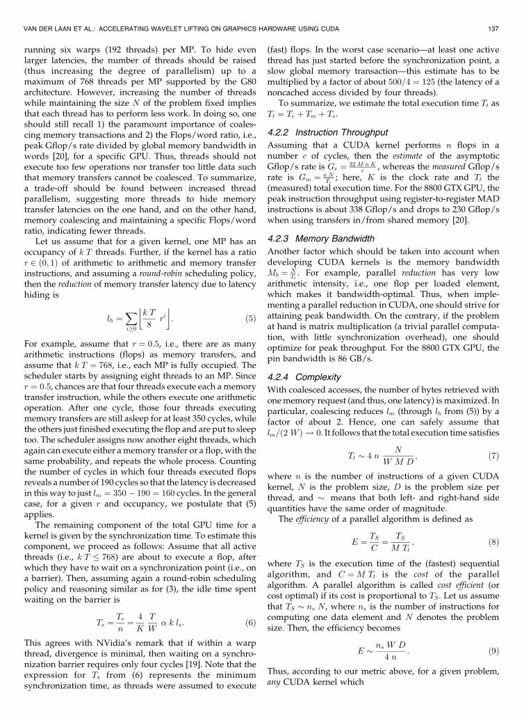
running six warps (192 threads) per MP. To hide evenlarger latencies, the number of threads should be raised(thus increasing the degree of parallelism) up to amaximum of 768 threads per MP supported by the G80architecture. However, increasing the number of threadswhile maintaining the size N of the problem fixed impliesthat each thread has to perform less work. In doing so, oneshould still recall 1) the paramount importance of coales-cing memory transactions and 2) the Flops/word ratio, i.e.,peak Gflop/s rate divided by global memory bandwidth inwords [20], for a specific GPU. Thus, threads should notexecute too few operations nor transfer too little data suchthat memory transfers cannot be coalesced. To summarize,a trade-off should be found between increased threadparallelism, suggesting more threads to hide memorytransfer latencies on the one hand, and on the other hand,memory coalescing and maintaining a specific Flops/wordratio, indicating fewer threads.

Let us assume that for a given kernel, one MP has anoccupancy of k T threads. Further, if the kernel has a ratior 2 ð0; 1Þ of arithmetic to arithmetic and memory transferinstructions, and assuming a round-robin scheduling policy,then the reduction of memory transfer latency due to latencyhiding is

lh ¼Xi�0

k T

8ri

� �: ð5Þ

For example, assume that r ¼ 0:5, i.e., there are as manyarithmetic instructions (flops) as memory transfers, andassume that k T ¼ 768, i.e., each MP is fully occupied. Thescheduler starts by assigning eight threads to an MP. Sincer ¼ 0:5, chances are that four threads execute each a memorytransfer instruction, while the others execute one arithmeticoperation. After one cycle, those four threads executingmemory transfers are still asleep for at least 350 cycles, whilethe others just finished executing the flop and are put to sleeptoo. The scheduler assigns now another eight threads, whichagain can execute either a memory transfer or a flop, with thesame probability, and repeats the whole process. Countingthe number of cycles in which four threads executed flopsreveals a number of 190 cycles so that the latency is decreasedin this way to just lm ¼ 350� 190 ¼ 160 cycles. In the generalcase, for a given r and occupancy, we postulate that (5)applies.

The remaining component of the total GPU time for akernel is given by the synchronization time. To estimate thiscomponent, we proceed as follows: Assume that all activethreads (i.e., k T � 768) are about to execute a flop, afterwhich they have to wait on a synchronization point (i.e., ona barrier). Then, assuming again a round-robin schedulingpolicy and reasoning similar as for (3), the idle time spentwaiting on the barrier is

Ts ¼Ten¼ 4

K

T

W� k ls: ð6Þ

This agrees with NVidia’s remark that if within a warpthread, divergence is minimal, then waiting on a synchro-nization barrier requires only four cycles [19]. Note that theexpression for Ts from (6) represents the minimumsynchronization time, as threads were assumed to execute

(fast) flops. In the worst case scenario—at least one activethread has just started before the synchronization point, aslow global memory transaction—this estimate has to bemultiplied by a factor of about 500=4 ¼ 125 (the latency of anoncached access divided by four threads).

To summarize, we estimate the total execution time Tt asTt ¼ Te þ Tm þ Ts.

4.2.2 Instruction Throughput

Assuming that a CUDA kernel performs n flops in anumber c of cycles, then the estimate of the asymptoticGflop/s rate is Ge ¼ 32 M n K

c , whereas the measured Gflop/srate is Gm ¼ n N

Tt; here, K is the clock rate and Tt the

(measured) total execution time. For the 8800 GTX GPU, thepeak instruction throughput using register-to-register MADinstructions is about 338 Gflop/s and drops to 230 Gflop/swhen using transfers in/from shared memory [20].

4.2.3 Memory Bandwidth

Another factor which should be taken into account whendeveloping CUDA kernels is the memory bandwidthMb ¼ N

Tt. For example, parallel reduction has very low

arithmetic intensity, i.e., one flop per loaded element,which makes it bandwidth-optimal. Thus, when imple-menting a parallel reduction in CUDA, one should strive forattaining peak bandwidth. On the contrary, if the problemat hand is matrix multiplication (a trivial parallel computa-tion, with little synchronization overhead), one shouldoptimize for peak throughput. For the 8800 GTX GPU, thepin bandwidth is 86 GB/s.

4.2.4 Complexity

With coalesced accesses, the number of bytes retrieved withone memory request (and thus, one latency) is maximized. Inparticular, coalescing reduces lm (through lh from (5)) by afactor of about 2. Hence, one can safely assume thatlm=ð2 WÞ ! 0. It follows that the total execution time satisfies

Tt � 4 nN

W M D; ð7Þ

where n is the number of instructions of a given CUDAkernel, N is the problem size, D is the problem size perthread, and � means that both left- and right-hand sidequantities have the same order of magnitude.

The efficiency of a parallel algorithm is defined as

E ¼ TSC¼ TSM Tt

; ð8Þ

where TS is the execution time of the (fastest) sequentialalgorithm, and C ¼M Tt is the cost of the parallelalgorithm. A parallel algorithm is called cost efficient (orcost optimal) if its cost is proportional to TS . Let us assumethat TS � ns N , where ns is the number of instructions forcomputing one data element and N denotes the problemsize. Then, the efficiency becomes

E � ns W D

4 n: ð9Þ

Thus, according to our metric above, for a given problem,any CUDA kernel which


1. uses coalesced memory transfers (i.e., lm=ð2 W Þ ! 0 isenforced),

2. avoids thread divergence (so that our Ts estimatefrom (6) applies),

3. minimizes transfers from global memory, and4. has an instruction count n proportional to ðns W DÞ

is cost-efficient. Of course, the smaller n is, the more efficientthe kernel becomes.

4.3 Parallel Wavelet Lifting

Earlier parallel methods for wavelet lifting [13] assumed anMPI architecture with processors that have their ownmemory space. However, the CUDA architecture isdifferent. Each processor has its own shared memory areaof 16 KB, which is not enough to store a significant part ofthe data set. As explained above, each processor is allocateda number of threads that run in parallel and cansynchronize. The processors have no way to synchronizewith each other, beyond their invocation by the host.

This means that data parallelism has to be used, andmoreover, the data set has to be split into parts that can beprocessed as independently as possible, so that each chunk ofdata can be allocated to a processor. For wavelet lifting, exceptfor the Haar [4] transform, this task is not trivial, as theimplied data reuse in lifting also requires the coefficients justoutside the delimited block to be updated. This could besolved by duplicating part of the data in each processor.Wavelet bases with a large support will, however, need moredata duplication. If we want to do a multilevel transform,each level of lifting doubles the amount of duplicated workand data. With the limited amount of shared memoryavailable in CUDA, this is not a feasible solution.

As kernel invocations introduce some overhead each time,we should also try to do as much work within one kernel aspossible so that the occupancy of the GPU is maximized. Thesliding window approach enables us (in the case of separablewavelets) to keep intermediate results longer in sharedmemory, instead of being written to global memory.

4.4 Separable Wavelets

For separable wavelet bases in 2D, it is possible to split theoperation into a horizontal and a vertical filtering step. Foreach filter level, a horizontal pass performs a 1D transformon each row, while a vertical pass computes a 1D transformon each column. This lends itself to easy parallelization:each row can be handled in parallel during the horizontalpass, and then, each column can be handled in parallelduring the vertical pass. In CUDA, this implies the use oftwo kernels, one for each pass. The simple solution wouldbe to have each block process a row with the horizontalkernel, while in the vertical step, each block processes acolumn. Each thread within these blocks can then filter anelement. We will discuss better specific algorithms for bothpasses in the upcoming sections.

4.5 Horizontal Pass

The simple approach mentioned in the previous sectionworks very well for the horizontal pass. Each block starts byreading a line into shared memory using so-called coalescedreads from device memory, executes the lifting steps in-place in fast shared memory, and writes back the resultusing coalesced writes. This amounts to the following steps:

1. Read a row from device memory into sharedmemory.

2. Duplicate border elements (implement boundarycondition).

3. Do a 1D lifting step on the elements in sharedmemory.

4. Repeat steps 2 and 3 for each lifting step of thetransform.

5. Write back the row to device memory.

As each step is dependent on the output in shared memoryof the previous step, the threads within the block have tobe synchronized every time before the next step can start.This ensures that the previous step did finish and wroteback its work.

Fig. 4 shows the configuration of the CUDA executionmodel for the horizontal step. Without loss of generality,assume that N ¼ w � h integers are lifted at level i. Note thatif the lifting level i ¼ 0, then w and h are the dimensions ofthe input image. For this step, a number B ¼ h of threadblocks are used, with T threads per block. Thus, each threadperforms computations on w=T integers. In the figure, blackquads illustrate locations which are processed by the threadwith id 0. Neither the number nor the positions of thesequads need to correspond to the actual number andpositions of locations where computations are performed,i.e., they are solely used for illustration purposes.

By reorganizing the coefficients [21], we can achievehigher efficiency for successive levels after the firsttransformation. If the approximation and detail coefficientsare written back in interleaved form, as is usually the casewith wavelet lifting, the reading step for the next level willhave to read the approximation coefficients of the previouslevel in interleaved form. These reads cannot be coalesced,resulting in low-memory performance. To still be able tocoalesce, one writes the approximation and detail coeffi-cients back to separate halves of the memory. This willresult in a somewhat different memory layout for subbands(Fig. 5), but this could be reorganized if needed. Manycompression algorithms require the coefficients stored persubband anyhow, in which case this organization isadvantageous.

4.6 Vertical Pass

The vertical pass is more involved. Of course, it is possible touse the same strategy as for the horizontal pass, substitutingrows for columns. But this is far from efficient. Reading acolumn from the data would amount to reading one valueper row. As only consecutive reads can be coalesced into oneread, these are all performed individually. The processing


Fig. 4. Horizontal lifting step. h thread blocks are created, eachcontaining T threads; each thread performs computations on N=ðhT Þ ¼w=T data. Black quads illustrate input for the thread with id 0. Here, wand h are the dimensions of the input and N ¼ w � h.

steps would be the same as for the horizontal pass, after

which writing back is again very inefficient.We can gain a 10 times speedup by using coalesced

memory access. Instead of having each block process a

column, we make each block process multiple columns by

dividing the image into vertical “slabs,” see Fig. 6. Within a

block, threads are organized into a 2D grid of size Vx � Vy ,

instead of a 1D one, as in the horizontal step. The numberS of

columns in each slab is a multiple of Vx such that the resulting

number of slab rows can still be coalesced, and has the height

of the image. Each thread block processes one of the slabs, i.e.,

S=Vx � h=Vy data. Using this organization, a thread can do a

coalesced read from each row within a slab, do filtering in

shared memory, and do a coalesced write to each slab row.Another problem arises here, namely, that the shared

memory in CUDA is not large enough to store all columns

for any sizable data set. This means that we cannot read and

process the entire slab at once. The solution that we found is

to use a sliding window within each slab, see Fig. 7a. This

window needs to have dimensions so that each thread in

the block can transform a signal element, and additional

space to make sure that the support of the wavelet does not

exceed the top or bottom of the window. To determine the

size of the window needed, how much to advance, and at

which offset to start, we need to look at the support of each

of the lifting steps.In Fig. 7a, height is the height of the working area. As

each step updates either odd or even rows within a slab,

each row of threads updates one row in each lifting step.

Therefore, a good choice is to set it to two times the number

of threads in the vertical direction. Similarly, width should

be a multiple of the number of threads in the horizontal

direction, and the size of a row should be a multiple of the

coalescable size. In the figure, rows in the top area have

been fully computed, while rows in the overlap area still

need to go through at least one lifting step. The rows in the

working area need to go through all lifting steps, while

rows in the bottom area are untouched except as border

extension. The sizes of overlap, top, and bottom depend on

the chosen wavelet. We will elaborate on this later.

4.6.1 The Algorithm

Algorithm 1 shows the steps for the vertical lifting pass.Three basic operations are used: read copies rows fromdevice memory into shared memory, write copies rows fromshared memory back to device memory, and copy transfersrows from shared memory to another place in sharedmemory. The shared memory window is used as a cache,and to manage this, we keep a read and a write pointer. Theread pointer inrow indicates where to read from, the writepointer outrow indicates where to write back. After reading,we advance the read pointer; after writing, we advance thewrite pointer. Both are initialized to the top of the slab at thebeginning of the kernel (lines 1 and 2 of Algorithm 1).

Algorithm 1. The sliding window algorithm for the vertical

wavelet lifting transform (see Section 4.6). Here top,overlap, height, bottom are the length parameters of the

sliding window (see Fig. 7), and h is the number of rows of

the data set. The pointer inrow indicates where to read from,

the pointer outrow indicates where to write back.

1: inrow 0 {initialize read pointer}

2: outrow 0 {initialize write pointer}

3: windows ðh� height� bottomÞ=height {number of

times window fits in slab}4: leftover ðh� height� bottomÞ%height

{remainder}

5: read(heightþ bottom from row inrow to row

topþ overlap) {copy from global to shared memory}

6: inrow inrowþ heightþ bottom {advance read

pointer}

7: transformTop() {apply vertical wavelet lifting to rows in

shared memory}8: write(height� overlap from row topþ overlap to

row outrow) {write transformed rows back to global

memory}

9: outrow outrowþ height� overlap {advance write

pointer}

10: for i ¼ 1 to windows do {advance sliding window through

slab and repeat above steps}

11: copy(topþ overlapþ bottom from row height to

row 0)

12: read (height from row inrow to row topþ overlap

þ bottom)

13: inrow inrowþ height

14: transformBlock() {vertical wavelet lifting}


(a) (b)

Fig. 7. (a) The sliding window used during the vertical pass for separablewavelets. (b) Advancing the sliding window: the next window is alignedat the bottom of the previous one, taking the overlap area into account.

Fig. 5. Wavelet lifting for a row of data, representing the result ininterleaved (top) and deinterleaved (bottom) form. Here, xi and yi arethe approximation and detail bands at level i.

Fig. 6. Vertical lifting step. w=S blocks are created, each containingT ¼ Vx � Vy threads; each thread performs computations on S=Vx � h=Vydata. Black quads illustrate input for the thread with id ð0; 0Þ, whereasvertical lines depict boundaries between image-high slabs.

15: write(height from row top to row outrow)

16: outrow outrowþ height

17: end for

18: copy(topþ overlapþ bottom from row height to

row 0)

19: read(leftover from row inrow to row

topþ overlapþ bottom)

20: transformBottom() {satisfy bottom boundary condition}21: write(leftoverþ overlapþ bottom from row top to

row outrow)

The first block has to be handled differently because weneed to take the boundary conditions into account. So,initially, rows are copied from the beginning of the slab toshared memory, filling it from a certain offset to the end(line 5). Next, we apply a vertical wavelet lifting transform(transformTop, line 7) to the rows in shared memory (itmay be required to leave some rows at the end untouchedfor some of the lifting steps, depending on their support; wewill elaborate on this in the next section). After this, wewrite back the fully transformed rows from shared memoryto device memory (line 8). Then, for each block, the bottompart of the shared memory is copied to the top part (Fig. 7b),in order to align the next window at the bottom of theprevious one, taking the overlap area into account (line 11).The rest of the shared memory is filled again by copyingrows from the current read pointer of the slab (line 12).

Further, we apply a vertical wavelet lifting transform(transformBlock, line 14) to the rows in the working area.This does not need to take boundary conditions intoaccount as the top and bottom are handled specificallywith transformTop and transformBottom. Then, heightrows are copied from shared memory row top to thecurrent write pointer (line 15). This process is repeated untilwe have written back the entire slab, except for the lastleftover part. When finishing up (line 20), we have to becareful to satisfy the bottom boundary condition.

4.6.2 Example

We will discuss the Deslauriers-Dubuc ð13; 7Þ wavelet as anexample [22]. This example was chosen because it repre-sents a nontrivial, but still compact enough case of thealgorithm, that we can go through step by step. The filterweights for the two lifting steps of this transform are shownin Table 2. Both the prediction and update steps depend ontwo coefficients before and after the signal element to becomputed. Fig. 8 shows an example of the performedcomputations. For this example, we choose top ¼ 3,

overlap ¼ 2, height ¼ 8, and bottom ¼ 3. This is a toyexample, as, in practice, height will be much larger whencompared to the other parameters.

Starting with the first window at the start of the data set,step 1 (first column), the odd rows of the working area (offset1; 3; 5; 7) are lifted. The lifted rows are marked with a cross,and the rows they depend on are marked with a bullet. In step2 (second column), the even rows are lifted. Again, the liftedrows are marked with a cross, and the dependencies aremarked with a bullet. As the second step is dependent on thefirst, we cannot lift any rows that are dependent on values thatwere not yet calculated in the last step. In Fig. 8, this would bethe case for row 6: this row requires data in rows 3, 5, 7, and 9,but row 9 is not yet available.

Here, the overlap region of rows comes in. As row 6 ofthe window is not yet fully transformed, we cannot write itback to device memory yet. So, we write everything up tothis row back, copy the overlapping area to the top, andproceed with the second window. In the second window,we again start with step 1. The odd rows are lifted, exceptfor the first one (offset 7) which was already computed, i.e.,rows 9, 11, 13, and 15 are lifted. Then, in step 2, we start atrow 6, i.e., three rows before the first step (row 9), but we dolift four rows.

After this, we can write the top eight rows back to devicememory and begin with the next window in exactly thesame way. We repeat this until the entire data set istransformed. By letting the second lifting step lag behindthe first, one can do the same number of operations in each,making optimal use of the thread matrix (which shouldhave a height of 4 in this case).

All separable wavelet lifting transforms, even those withmore than two lifting steps, or with differently sizedsupports, can be computed in the same way. The transformcan be inverted by running the steps in reverse order andflipping the signs of the filter weights.

4.7 3D and Higher Dimensions

The reason that the horizontal and vertical passes areasymmetric is because of the coalescing requirement forreads and writes. In the horizontal case, an entire line of thedata set could be processed at a time. In the vertical case,the data set was horizontally split into image-high slabs.This allowed the slabs to be treated independently andprocessed using a sliding window algorithm that uses


Fig. 8. The vertical pass for the Deslauriers-Dubuc ð13; 7Þ [22] wavelet.Lifted rows in each step are marked with a cross, and dependent rowsare marked with a bullet.

TABLE 2Filter Weights of the Two Lifting Steps for the

Deslauriers-Dubuc ð13; 7Þ [22] Wavelet

The current element being updated is marked with �.

coalesced reads and writes to access lines of the slab. Aconsecutive, horizontal span of values is stored at con-secutive addresses in memory. This does not extendsimilarly to vertical spans of values, these will be separatedby an offset at least the width of the image, known as therow pitch. As a slab is a rectangular region of the image of acertain width that spans the height of the image, it will berepresented in memory by an array of consecutive spans ofvalues, each separated by the row pitch.

When adding an extra dimension, let us say z, the volumeis stored as an array of slices. In a span of values orientedalong this dimension, each value is separated in memory byan offset that we call the slice pitch. By orienting the slabs inthe xz-plane instead of the xy-plane, and thus, using the slicepitch instead of the row pitch as offset between consecutivespans of values, the same algorithm as in the vertical casecan be used to do a lifting transform along this dimension.To verify our claim, we implemented the method justdescribed, and report results in Section 5.2.7. More thanthree dimensions can be handled similarly, by orienting theslabs in the Dix plane (where Di is the dimension i) andusing the pitch in that dimension instead of the row pitch.

5 RESULTS

We first present a broad collection of experimental results.This is followed by a performance analysis which providesinsight in the results obtained, and also shows that the designchoices we made closely match our theoretical predictions.

The benchmarks in this section were run on a machinewith a AMD Athlon 64 X2 Dual Core Processor 5200+ and aNVidia GeForce 8800 GTX 768MB graphics card, usingCUDA version 2.1 for the CUDA programs. All reportedtimings exclude the time needed for reading and writingimages or volumes from and to disc (both for the CPU andGPU versions).

5.1 Wavelet Filters Used for Benchmarking

The wavelet filters that we used in our benchmarks areinteger-to-integer versions (unnormalized) of the Haar [4],Deslauriers-Dubuc ð9; 7Þ [22], Deslauriers-Dubuc ð13; 7Þ [22],Le Gall ð5; 3Þ [23] (integer approximation of) Daubechiesð9; 7Þ [2], and the Fidelity wavelet—a custom wavelet with alarge support [24]. In the filter naming convention ðm;nÞ, mrefers to the length of the analysis low-pass and n to theanalysis high-pass filters in the conventional waveletsubband filtering model, in which a convolution is appliedbefore subsampling. They do not reflect the length of thefilters used in the lifting steps, which operate in thesubsampled domain. The implementation only involvesinteger addition and multiplication, and integer division bypowers of 2 (bit-shifting) (cf. Section 3.2). The coefficients ofthe lifting filters can be found in [24].

5.2 Experimental Results and Comparison to OtherMethods

5.2.1 Comparison of 2D Wavelet Lifting,

GPU versus CPU

First, we emphasize that the accuracies of the GPU and CPUimplementations are the same. Because only integeroperations are used (cf. Section 5.1), the results are identical.

We compared the speed of performing various wavelettransforms using our optimized GPU implementation, to anoptimized wavelet lifting implementation on the CPU,called Schrodinger [24]. The latter implementation makesuse of vectorization using the MMX and SSE instruction setextensions, thus can be considered close to the maximumthat can be achieved on the CPU with one core.

Table 3 shows the timings of both our GPU-acceleratedimplementation and the Schrodinger implementation whencomputing a three-level transform with various wavelets ofa 1;920� 1;080 image consisting of 16-bit samples. As it isbetter from an optimization point of view to have a tailoredkernel for each wavelet type than to have a single kernelthat handles everything, we used a code generationapproach to create specific kernels for the horizontal andvertical pass for each of the wavelets. Both the analysis(forward) and synthesis (inverse) transforms are bench-marked. We observe that speedups by a factor of 10-14 arereached, depending on the type of wavelet and the directionof the transform. The speedup factor appears to be roughlyproportional to the length of the filters. The Haar wavelet isan exception, since the overlap problem does not arise inthis case (the filter length being just 2), which explains thelarger speedup factor.

To demonstrate the importance of coalesced memoryaccess in CUDA, we also performed timings using a trivialCUDA implementation of the Haar wavelet that uses thesame algorithm for the vertical step as for the horizontalstep, instead of our sliding window algorithm. Note thatthis method can be considered an improved (using cache)row-column, hardware-based strategy, see Section 2. Whileour algorithm processes an image in 0.80 milliseconds, thetrivial algorithm takes 15.23, which is almost 20 timesslower. This is even slower than performing the transfor-mation on the CPU.

Note that the timings in Table 3 do not include thetime required to copy the data from (2.4 ms) or to (1.6 ms)the GPU.

5.2.2 Vertical Step via Transpose Method

Another method that we have benchmarked consists inreusing the horizontal step as vertical step by using a“transpose” method. Here, the matrix of wavelet coefficientsis transposed after the horizontal pass, the algorithm for thehorizontal step is applied, and the results are transposedback. The results are shown in columns 3 and 4 of Table 3.Even though the transpose operation in CUDA is efficient andcoalescable and this approach is much easier to implement,the additional passes over the data reduce performance quiteseverely. Another drawback of this method is that transposi-tion cannot be done in-place efficiently (in the general case),which doubles the required memory, so that the advantage ofusing the lifting strategy is lost.

5.2.3 Comparison of Horizontal and Vertical Steps

Table 4 shows separate benchmarks for the horizontal andvertical steps, using various wavelet filters. From theseresults, one can conclude that the vertical pass is notsignificantly slower (and in some cases even faster) than thehorizontal pass, even though it performs more elaboratecache management, see Algorithm 1.


5.2.4 Timings for 16-Bit versus 32-Bit Integers

We also benchmarked an implementation that uses 32-bitintegers, see Table 5. For small wavelets like Haar, thetimings for 16- and 32-bit differ by a factor of around 1.5,whereas for large wavelets, the two are quite close. This isprobably because the smaller wavelet transforms are morememory-bound and the larger wavelets are more compute-bound; hence, the increased memory bandwidth does notaffect the performance significantly.

5.2.5 Comparison of 2D Wavelet Lifting on GPU, CUDA

versus Fragment Shaders

We also implemented the algorithm of Tenllado et al. [12] forwavelet lifting using conventional fragment shaders andperformed timings on the same hardware. A three-levelDaubechies ð9; 7Þ forward wavelet transform was applied toa 1;920� 1;080 image, which took 5.99 milliseconds. Incomparison, our CUDA-based implementation (see Table 3)does the same in 2.05 milliseconds, which is about 2.9 timesfaster. This speedup probably occurs because our methodeffectively makes use of CUDA shared memory to compute

intermediate lifting steps, conserving GPU memory band-width, which is the bottleneck in the Tenllado method.Another drawback that we noticed while implementing themethod is that an important advantage of wavelet lifting, i.e.,that it can be done in place, appears to have been ignored.This is possibly due to an OpenGL restriction by which it isnot allowed to use the source buffer as destination, the sameresult is achieved by alternating between two halves of abuffer, resulting in a doubling of memory usage.

Fig. 9 further compares the performance of the Schro-dinger CPU implementation [12] and our CUDA-acceler-ated method. A three-level Daubechies ð9; 7Þ forwardwavelet decomposition was applied to images of differentsizes, and the computation time was plotted versus imagesize in a log-log graph. This shows that our method is fasterby a constant factor, regardless of the image size. Even forsmaller images, our CUDA-accelerated implementation isfaster than the CPU implementation, whereas the shader-based method of Tenllado is slower for 256� 256 images,due to OpenGL rendering and state setup overhead. CUDAkernel calls are relatively lightweight, so this problem doesnot arise in our approach. For larger images, the overhead


TABLE 4Performance of Our GPU implementation on 16-Bit Integers,

Separate Timings of Horizontal and Vertical Steps ona One-Level Decomposition of a 1;920� 1;080 Image

TABLE 3Performance of Our CUDA GPU Implementation of 2D Wavelet Lifting (Column 5) Compared to an Optimized CPU Implementation

(Column 2) and a CUDA GPU Transpose Method (Column 3, See Text), Computing a Three-Level Decomposition of a1;920� 1;080 Image for Both Analysis and Synthesis Steps

TABLE 5Performance of Our GPU Implementation on 16 versus 32-Bit

Integers (Three-Level Transform, 1;920� 1;080 Image)

averages out, but as the method is less bandwidth efficient,it remains behind by a significant factor.

5.2.6 Comparison of Lifting versus Convolution in CUDA

Additionally, we compared our method to a convolution-based wavelet transform implemented in CUDA, one thatuses shared memory to perform the convolution plusdownsampling (analysis), or upsampling plus convolution(synthesis) efficiently. On a 1;920� 1;080 image, for a three-level transform with the Daubechies ð9; 7Þ wavelet, thefollowing timings are observed: 3.4 ms for analysis and5.0 ms for synthesis. The analysis is faster than the synthesisbecause it requires less computations—only half of thecoefficients have to be computed, while the other half arediscarded in the downsampling step. Compared to the 2.0 msof our own method for both transforms, this is significantlyslower. This matches the expectation that a speedup factor of1.5-2 can be achieved when using lifting [4].

5.2.7 Timings for 3D Wavelet Lifting in CUDA

Timings for the 3D approach outlined in Section 4.7 aregiven in Table 6. A three-level transform was applied to a5123 volume, using various wavelets. The timings arecompared to the same CPU implementation as before,

extended to 3D. The numbers show that the speedups thatcan be achieved for higher dimensional transforms areconsiderable, especially for the larger wavelets such asDeslauriers-Dubuc ð13; 7Þ or Fidelity.

5.2.8 Summary of Experimental Results

Compared to an optimized CPU implementation, we haveseen performance gains of up to nearly 14 times for 2D andup to 25 times for 3D images by using our CUDA-basedwavelet lifting method. Especially for the larger wavelets,the gains are substantial. When compared to the trivialtranspose-based method, our method came out about twotimes faster over the entire spectrum of wavelets. Whenregarding computation time versus image size, our GPU-based wavelet lifting method was measured to be the fastestof three methods for all image sizes, with the factor mostlyindependent of the image size.

5.3 Performance Analysis

We analyze the performance of our GPU implementation,according to the metrics from Section 4.2, for performing onelifting (analysis) step. Without loss of generality, we discussthe Deslauriers-Dubuc ð13; 7Þ wavelet (cf. Section 4.6). Oursystematic approach consists first in explaining the totalexecution time, throughput, and bandwidth of our method,and then, in discussing the design decisions we made. Theoverhead of data transfer between CPU and GPU wasexcluded, since the wavelet transform is usually part of alarger processing pipeline (such as a video codec), of whichmultiple steps can be carried out on the GPU.

5.3.1 Horizontal Step

The size of the input data set is N ¼ w � h ¼ 1;920 � 1;080two-byte words. We set T ¼ 256 threads per block, andgiven the number of registers and the size of the sharedmemory used by our kernel, NVidia’s occupancy calcu-lator indicates that k ¼ 3 blocks are active per MP, suchthat each MP is fully occupied (i.e., k T ¼ 768 threads willbe scheduled); the number of thread blocks for thehorizontal step is B ¼ 1;080. Given that the 8800 GTX


(a)(a)

(b)

Fig. 9. Computation time versus image size for various liftingimplementations; three-level Daubechies ð9; 7Þ forward transform.(a) The Schrodinger CPU implementation [12] and our CUDA-accelerated method in a log-log plot. (b) Just the two GPU methods ina linear plot.

TABLE 6Performance of Our GPU Lifting Implementation in 3D,

Compared to an Optimized CPU Implementation;a Three-Level Decomposition for Both Analysis and

Synthesis Is Performed on a 5123 Volume

GPU has M ¼ 16 MPs, it follows that � ¼ 23, seeSection 4.2. Further, we used decuda (a disassembler ofGPU binaries; see http://wiki.github.com/laanwj/decuda)to count the number and type of instructions performed.After unrolling the loops, we found that the kernel has309 instructions, 182 of which are arithmetic operations inlocal memory and registers, 15 instructions are half-width(i.e., instruction code is 32-bit wide), 82 are memorytransfers, and 30 are other instructions (mostly typeconversions). Assuming that half-width instructions havea throughput of two cycles, and others take four cycles perwarp, and since the clock rate of this device is K ¼ 1:35GHz, the asymptotic execution time is Te ¼ 0:48 ms. Here,we assumed that the extra overhead due to rescheduling isnegligible, as was confirmed by our experiments.

For the transfer time, we first computed the ratio ofarithmetic to arithmetic-and-transfers instructions, which isr ¼ 0:67. Thus, from (5), it follows that as many as 301 cyclescan be spared due to latency hiding. As the amount ofshared memory used by the kernel is relatively small (i.e.,3� 3:75 KB used out of 16 KB per MP) and the size of the L2cache is about 12 KB per MP [20], we can safely assume thatthe latency of a global memory access is about 350 cycles sothat lm ¼ 49 cycles. Since m ¼ 4 (i.e., two 2-byte words arecoalesced), the transfer time is Tm ¼ 0:15 ms. Note that astwo MPs also share a small but faster L1 cache of 1.5 KB, thereal transfer time could be even smaller than our estimate.Moreover, as we also included in our counting sharedmemory transfers (whose latency is at least 10 times smallerthan that of global memory), the real transfer time shouldbe much smaller than its estimate.

According to our discussion in Section 4.5, five synchro-nization points are needed to ensure data consistencybetween individual steps. For one barrier, in the ideal case,the estimated waiting time is Ts ¼ 1:65 �s; thus, the totaltime is about 8:25 �s. In the worst case, Ts ¼ 0:2 ms so thatthe total time can be as large as 1 ms.

To summarize, the estimated execution time for thehorizontal step is about Tt ¼ 0:63 ms, neglecting thesynchronization time. Comparing this result with themeasured one from Table 4, one sees that the estimatedtotal time is 0.16 ms larger than the measured one. Probably,this is due to L1 caching contributing to a further decrease ofTm. However, It is essential that the total time is dominatedby the execution time, indicating a compute-bound kernel.As the timing remains essentially the same (cf. Tables 3 and5) when switching from 2-byte words to 4-byte words data,this further strengthens our finding.

The measured throughput is Gm ¼ 98 Gflop/s, whereasthe estimated one is Ge ¼ 104 Gflop/s, indicating, onaverage, an instruction throughput of about 100 Gflop/s.Note that with some abuse of terminology, we refer to flops,when, in fact, we mean arithmetic instructions on integers.The measured bandwidth is Mb ¼ 8:8 GB/s, i.e., we arequite far from the pin-bandwidth (86 GB/s) of the GPU;thus, one can conclude again that our kernel is indeedcompute-bound. This conclusion is further supported bythe fact that the flop-to-byte ratio of the GPU is 5, while inour case, this ratio is about 11. The fact that the kernel doesnot achieve the maximum throughput (using shared

memory) of about 230 Gflop/s is most likely due to thefact that the synchronization time cannot simply beneglected and seems to play an important role in theoverall performance.

Let us now focus on the design choices we have made.Using T ¼ 256 threads per block amounts to optimal timeslicing (latency hiding), see discussion above and inSection 4.2, while we are still able to coalesce memorytransfers. To decrease the synchronization time, lighterthreads are suggested implying that their number shouldincrease, while maintaining a fixed size of the problem.NVidia’s performance guidelines [19] suggest that theoptimal number of threads per block should be a multipleof 64. The next higher than 256 multiple of 64 is 320.Unfortunately, using 320 threads per block means that atmost two blocks can be allocated to one MP, and thus, theMP will not be fully occupied. This, in turn, implies that animportant amount of idle cycles spent on memory transferscannot be saved, rendering the method less optimal withrespect to time slicing. Accordingly, our choice of T ¼ 256threads per block is optimal. Further, our choice on thenumber of blocks also fulfills NVidia’s guidelines withrespect to current and future GPUs, see [19].

5.3.2 Vertical Step

While conceptually more involved than the horizontal step,the overall performance figure for the vertical step is rathersimilar to the horizontal one. The CUDA configuration forthis kernel is as follows:. Each 2D thread block contains anumber of 16� 8 ¼ 128 threads, while the number ofcolumns within each slab is S ¼ 32, see Fig. 6. Thus, sincethe input consists of 2-byte words, each thread performscoalesced memory transfers of m ¼ 4 bytes, similar to thehorizontal step. As the number of blocks is w=S ¼ 60, k ¼ 4(i.e., four blocks are scheduled per MP) and the kernel takes39,240 cycles per warp to execute, the execution time for thevertical step is Te ¼ 0:46.

Unlike the horizontal step, now r ¼ 0:83 so that no lessthan 352 cycles can be spared in global memory transaction.Note that when computing r, we only counted globalmemory transfers, as in this case, more, much faster sharedmemory transfers take place, see Algorithm 1. As the sharedmemory usage is only 4� 1:8 KB, this suggests that theoverhead due to slow accesses to global memory can beneglected so that the transfer time Tm can be neglected. Thewaiting time is Ts ¼ 0:047 �s, and there are 344 synchroni-zation points for the vertical step kernel so that the totaltime is about 15:6 �s. In the worst case, this time can be aslarge as 1.9 ms. Thus, as Tt ¼ 0:46 (without waiting time),our estimate is very close to the measured execution timefrom Table 4—this being, in turn, the same as that of thehorizontal step. Finally, both the measured and estimatedthroughputs are comparable to their counterparts of thehorizontal step.

Note that compared to the manually tuned, optimallydesigned matrix multiplication algorithm of [20] which isable to achieve a maximum throughput of 186 Gflop/s, theperformance of 100 Gflop/s of our lifting algorithms maynot seem impressive. However, one should keep in mindthat matrix multiplication is much easier to parallelizeefficiently, as it requires little synchronization. Unlike


matrix multiplication, the lifting algorithm requires a lotmore synchronization points to ensure data consistencybetween steps, as the transformation is done in-place.

The configuration we chose for this kernel is 16� 8 ¼ 128

threads per block and w=S ¼ 60 thread blocks. This resultsin an occupancy of 512 threads per MP, which may seemless optimal. However, to increase the number of threadsper block to 192 (next larger multiple of 64, see above)would mean that either we cannot perform essential,coalesced memory accesses, or that extra overhead due tothe requirements of the moving-window algorithm wouldhave to be accommodated. Note that we verified thispossibility, but the results were unsatisfactory.

5.3.3 Complexity

Based on the formulas in Section 4.2, we can analyze thecomplexity of our problem. For any of the lifting steps usingthe Deslauriers-Dubuc ð13; 7Þ wavelet, considering that thenumber of flops per data element is ns ¼ 22 (20 multiply oradditions and two register shifts to increase accuracy), thenumerator of (9) becomes about 700 D. For the horizontalstep, D ¼ w=T ¼ 7:5 so that the numerator becomes about5,000. In this case, the number of cycles is about 1,250 so thatone can conclude that the horizontal step is indeed cost-

efficient. For the vertical step, D ¼ ðS hÞ=T ¼ 270 so that thenumerator in (9) becomes about 190,000, while the denomi-nator is 39,240. Thus, the vertical step is also cost-efficient,and actually, its performance is similar to that of thehorizontal step (because 5;000=1;250 190;000=39;240 5).Of course, this result was already obtained experimentally,see Table 4. Note that using vectorized MMX and SSEinstructions, the optimized CPU implementation (see Table 3)can be up to four times faster than our TS estimate above.However, even in this case, both our CUDA kernels are stillcost-efficient. Obviously, both steps are also work-efficient, astheir CUDA realizations do not perform asymptotically moreoperations than the sequential algorithm.

6 CONCLUSION

We presented a novel, fast wavelet lifting implementationon graphics hardware using CUDA, which extends to anynumber of dimensions. The method tries to maximizecoalesced memory access. We compared our method to anoptimized CPU implementation of the lifting scheme, toanother (non-CUDA-based) GPU wavelet lifting method,and also to an implementation of the wavelet transform inCUDA via convolution. We implemented our method bothfor 2D and 3D data. The method is scalable and was shownto be the fastest GPU implementation among the methodsconsidered. Our theoretical performance estimates turnedout to be in fairly close agreement with the experimentalobservations. The complexity analysis revealed that ourCUDA kernels are cost- and work-efficient.

Our proposed GPU algorithm can be applied in all caseswhere the Discrete Wavelet Transform based on the liftingscheme is part of a pipeline for processing large amounts ofdata. Examples are the encoding of static images, such as thewavelet-based successor to JPEG, JPEG2000 [25], or videocoding schemes [24], which we already considered in [26].

ACKNOWLEDGMENTS

The authors thank the anonymous reviewers for several

helpful suggestions to improve their paper. This research is

part of the “VIEW: Visual Interactive Effective Worlds”

program, funded by the Dutch National Science Foundation

(NWO), project no. 643.100.501.

REFERENCES

[1] M.A. Westenberg and J.B.T.M. Roerdink, “Frequency DomainVolume Rendering by the Wavelet X-Ray Transform,” IEEE Trans.Image Processing, vol. 9, no. 7, pp. 1249-1261, July 2000.

[2] I. Daubechies, Ten Lectures on Wavelets, vol. 61. Soc. for Industrialand Applied Math., 1992.

[3] S. Mallat, A Wavelet Tour of Signal Processing. Academic Press,1998.

[4] W. Sweldens, “The Lifting Scheme: A Construction of SecondGeneration Wavelets,” SIAM J. Math. Analysis, vol. 29, no. 2,pp. 511-546, 1998.

[5] I. Daubechies and W. Sweldens, “Factoring Wavelet Transformsinto Lifting Steps,” J. Fourier Analysis and Applications, vol. 4, no. 3,pp. 247-269, 1998.

[6] A.R. Calderbank, I. Daubechies, W. Sweldens, and B.-L. Yeo,“Wavelet Transforms That Map Integers to Integers,” Applied andComputational Harmonic Analysis, vol. 5, no. 3, pp. 332-369, 1998.

[7] E. Lindholm, J. Nickolls, S. Oberman, and J. Montrym, “NVIDIATesla: A Unified Graphics and Computing Architecture,” IEEEMicro, vol. 28, no. 2, pp. 39-55, Mar./Apr. 2008.

[8] M. Hopf and T. Ertl, “Hardware Accelerated Wavelet Transfor-mations,” Proc. EG/IEEE TCVG Symp. Visualization (VisSym ’00),pp. 93-103, May 2000.

[9] A. Garcia and H.W. Shen, “GPU-Based 3D Wavelet Reconstructionwith Tileboarding,” The Visual Computer, vol. 21, pp. 755-763, 2005.

[10] T.T. Wong, C.S. Leung, P.A. Heng, and J. Wang, “Discrete WaveletTransform on Consumer-Level Graphics Hardware,” IEEE Trans.Multimedia, vol. 9, no. 3, pp. 668-673, Apr. 2007.

[11] C. Tenllado, R. Lario, M. Prieto, and F. Tirado, “The 2D DiscreteWavelet Transform on Programmable Graphics Hardware,” Proc.Fouth IASTED Int’l Conf. Visualization, Imaging, and Image Proces-sing, 2004.

[12] C. Tenllado, J. Setoain, M. Prieto, L. Pinuel, and F. Tirado,“Parallel Implementation of the 2D Discrete Wavelet Transformon Graphics Processing Units: Filter Bank versus Lifting,” IEEETrans. Parallel and Distributed Systems, vol. 19, no. 3, pp. 299-310,Mar. 2008.

[13] W. Jiang and A. Ortega, “Parallel Architecture for the DiscreteWavelet Transform Based on the Lifting Factorization,” J. Paralleland Distributed Computing, vol. 57, no. 2, pp. 257-269, 1999.

[14] M. Angelopoulou, K. Masselos, P. Cheung, and Y. Andreopoulos,“Implementation and Comparison of the 5/3 Lifting 2d DiscreteWavelet Transform Computation Schedules on FPGAs,” J. SignalProcessing Systems, vol. 51, no. 1, pp. 3-21, 2008.

[15] N.D. Zervas, G.P. Anagnostopoulos, V. Spiliotopoulos, and Y.Andreopoulos, “Evaluation of Design Alternatives for the 2DDiscrete Wavelet Transform,” IEEE Trans. Circuits and Systems forVideo Technology, vol. 11, no. 12, pp. 1246-1262, Dec. 2001.

[16] M.Y. Chiu, K.-B. Lee, and C.-W. Jen, “Optimal Data Transfer andBuffering Schemes for JPEG 20000 Encoder,” Proc. IEEE WorkshopDesign and Implementation of Signal Processing Systems, pp. 177-182,2003.

[17] T. Acharya and C. Chakrabarti, “A Survey on Lifting-BasedDiscrete Wavelet Transform Architectures,” J. VLSI Signal Proces-sing Systems, vol. 42, no. 3, pp. 321-339, 2006.

[18] NVidia, CUDA Occupancy Calculator, http://developer.download.nvidia.com/compute/cuda/CUDA_Occupancy_calculator.xls,2009.

[19] NVIDIA Corporation, Compute Unified Device Architecture Pro-gramming Guide, http://developer.nvidia.com/cuda, 2010.

[20] V. Volkov and J. Demmel, “LU, QR and Cholesky FactorizationsUsing Vector Capabilities of GPUs,” technical report, Univ. ofCalifornia at Berkeley, 2008.

[21] S. Chatterjee and C.D. Brooks, “Cache-Efficient Wavelet Lifting inJPEG 2000,” Proc. IEEE Int’l Conf. Multimedia and Expo, pp. 797-800,2002.


[22] G. Deslauriers and S. Dubuc, “Symmetric Iterative InterpolationProcesses,” Constructive Approximation, vol. 5, no. 1, pp. 49-68, Dec.1989.

[23] D. LeGall and A. Tabatabai, “Sub-Band Coding of Digital ImagesUsing Symmetric Short Kernel Filters and Arithmetic CodingTechniques,” Proc. IEEE Int’l Conf. Acoustics, Speech and SignalProcessing, vol. 2, pp. 761-764, 1988.

[24] BBC Research, Dirac Specification 1.0.0pre7, http://dirac.sourceforge.net/specification.html, 2010.

[25] A.N. Skodras, C.A. Christopoulos, and T. Ebrahimi, “JPEG2000:The Upcoming Still Image Compression Standard,” PatternRecognition Letters, vol. 22, no. 12, pp. 1337-1345, 2001.

[26] W.J. van der Laan, A.C. Jalba, and J.B.T.M. Roerdink, “Accelerat-ing Wavelet-Based Video Coding on Graphics Hardware UsingCUDA,” Proc. Sixth Int’l Symp. Image and Signal Processing andAnalysis (ISPA ’09), pp. 614-619, Sept. 2009.

Wladimir J. van der Laan received the MScdegree in computing science in 2005 from theUniversity of Groningen, where he is currentlyworking toward the PhD degree at the JohannBernoulli Institute for Mathematics and ComputerScience. His research interests include computergraphics, visualization, and GPU computing.

Andrei C. Jalba received the BSc and MScdegrees in applied electronics and informationengineering from “Politehnica” University ofBucharest, Romania, in 1998 and 1999, respec-tively, and the PhD degree from the Institute forMathematics and Computing Science, Universityof Groningen, in 2004. Currently, he is anassistant professor at the Eindhoven Universityof Technology. His research interests includecomputer vision, pattern recognition, image

processing, and parallel computing.

Jos B.T.M. Roerdink received the MSc degreein theoretical physics from the University ofNijmegen, The Netherlands, in 1979, and thePhD degree from the University of Utrecht in1983. He was a postdoctoral fellow in the areaof stochastic processes at the University ofCalifornia, San Diego, from 1983 to 1985. Hejoined the Centre for Mathematics and Com-puter Science in Amsterdam. There he workedon image processing and tomographic recon-

struction from 1986 to 1992. He was appointed an associate professorin 1992 and a full professor in 2003, respectively, in the Institute forMathematics and Computing Science at the University of Groningen,where he currently holds a chair in Scientific Visualization andComputer Graphics. His current research interests include biomedicalvisualization, neuroimaging, and bioinformatics. He is a senior memberof the IEEE.

. For more information on this or any other computing topic,please visit our Digital Library at www.computer.org/publications/dlib.


Documents

University of Groningen Accelerating Wavelet Lifting on ... Wavelet Lifting on Graphics Hardware Using CUDA Wladimir J. van der Laan, Andrei C. Jalba, and Jos B.T.M. Roerdink,Senior