Embed Size (px)
Citation preview

MANIPULATION OF AUDIO IN THE WAVELETDOMAIN PROCESSING
A WAVELET STREAM USING PD
Institut für Elektronische Musik (IEM)
Graz, 2006
Raúl Díaz Poblete

2

ABSTRACT
El objetivo de este trabajo es investigar las posibilidadesdel uso en tiempo real de la transformada wavelet discreta conPure Data para el análisis / resíntesis de señales de audio.
Con esta intención he realizado un acercamiento conPure Data a un nuevo tipo de síntesis granular basada en latransformada wavelet: la resíntesis de una señal de audio apartir de sus coeficientes wavelet mediante una síntesis aditivade flujos de wavelets (una sucesión temporal de 'gránuloswavelet' para cada escala o banda de frecuencia que sonescalados por un factor de amplitud obtenido de loscoeficientes del análisis wavelet).
También he desarrollado otras aplicaciones de audiomediante la manipulación de los coeficientes wavelet paraestudiar las posibilidades de pitch shift, time stretch,ecualización y randomización de audio.
3

ABSTRACT
The aim of this work is to research the possibilities of usethe discrete wavelet transform in real-time with Pure Data foranalysis / resynthesis of audio signals.
With this intention I approached to a new sort ofgranular synthesis with Pure Data based on wavelettransform: resynthesis of an audio signal from its waveletcoefficients by means of an additive synthesis of waveletstreams (a temporal succession of 'wavelets grains' for eachscale or frequency level which are enveloped by an amplitudefactor obtained from wavelet analysis coefficients).
Another audio applications by means of waveletcoefficients manipulation have been developed to study thepossibilities of pitch shift, time stretch, equalization and audiorandomization.
4

ABSTRACT
Ziel der Arbeit ist die Möglichkeiten des Einsatzes derdiskreten Wavelet Transformation in Echtzeit mittels dergrafischen Programmiersprache Pure Data zu erforschen, umeine Analyse, Transformation und Resynthesis vonAudiosignalen zu realisieren.
Dazu wird eine neue Art eines granularen Synthesizermit Pure Data mit Wavlets als Samplebasis entwickelt. DieResynthese des Audiosignals von ihren Waveletkoeffizientenmittels additive wavelet Streams (zeitliche Abfolge von'wavelets grains' für jeden Frequenz Level errechnet aus denwavlet-Koeffizienten und damit deren Amplitudenskalierung).
Als Beispielsanwendungen der Manipulation derWaveletkoeffizienten wurde studien über die Möglichkeit vonTonhöhenveränderungen, zeitlicher Dehnung, Bandfilterungund Verschmierung von Zeitlichen Abfolgen der Wavletsrealisiert.
5

ACKNOWLEDGEMENTS
I'm deeply grateful to my supervisor, Winfried Ritsch, forall their help and support during the course of my research atIEM. I also thank Johannes Zmölnig and Thomas Musil for theirhelp in PD programming, and Robert Höldrich and BrigitteBergner for their flexibility and support in allowing the pursuitof this work. I'm also very grateful to Tom Schouten for hislibrary creb and his personal information about dwt~ external.
Finally, on a personal note, I thank my family and mybest friends for all the patience and support they have shownduring this time, which was fundamental in order to reach mypurposes.
6

TABLE OF CONTENTS
Abstract
Español .......................................................................... 3
Deutch ........................................................................... 4
English ........................................................................... 5
Acknoledgements ......................................................... 6
Table ofContents ....................................................................... 7
Chapter 1Wavelet Theoretical Background ................................ 11
1.1. Time-FrequencyRepresentations ................................................... 11
1.1.1. Short Time Fourier Transform .............. 11
1.1.2. Wavelet Transform ............................. 12
1.2. DWT: Discrete Wavelet Transform .................. 13
1.3. Lifting Scheme .............................................. 25
1.3.1. Haar Transform ................................. 25
1.3.2. Lifting Scheme .................................. 28
1.4. DWT in Pure Data: dwt~ external ................... 29
7

Chapter 2Wavelet Stream Additive Resynthesis ........................ 38
2.1. Wavelet Stream Additive Resynthesis ............... 38
2.2. PD implementation of a Wavelet Stream Additive Resynthesis ...................................... 39
2.2.1. Initializations ...................................... 42
2.2.2. DWT Analysis ..................................... 46
2.2.3. Coefficients list ................................... 47
2.2.4. Granulator ......................................... 48
2.2.5. Output ............................................. 50
Chapter 3Audio Manipulations in Wavelet Domain ................... 56
3.1.Audio Manipulations in Wavelet Domain and its PD Implementation ........................... 56
3.1.1. Audio input and dwt analysis .............. 58
3.1.2. Coefficients Manipulations .................. 63
3.1.3. Resynthesis and output sound ............ 64
3.2. Audio Modifications ...................................... 64
3.2.1. Stretch ........................................... 64
3.2.2. Shift ............................................... 65
3.2.3. Equalization .................................... 68
3.2.4. Randomization ..........................,..... 69
8
Chapter 4Conclusions and Future Research ............................... 72
Bibliography ............................................................... 73
9

10

Chapter 1
Wavelet Theoretical Background
In this chapter I will try to give a theoretical backgroundabout time-frequency representations focused on wavelettransform, which is the base of this work. This chapter doesn'twant to be a deep mathematical explanation, instead of this Iwill try to go into wavelets from an engineer point of view,more focused on signal processing. More mathematical detailscan be consulted in the related bibliography.
1.1. Time-Frequency Representations
Traditionally, signals of any sort have been representedin a temporal domain or in a frequencial domain. In the timedomain, we can look at an audio signal as magnitudes sampledat given times. In the frequency domain, an audio signal isrepresented as magnitudes of sinusoids at given frequencies.
But for audio analysis, it is quite interesting to have anoverview of an audio signal over both components, as inclassical music scores (temporal view of notes of differentpitch).
A time-frequency representation is a view of a signalrepresented over both time and frequency.
1.1.1. Short Time Fourier Transform
The Fourier Transform is a classical tool in signalprocessing which breaks down a signal into its constituentsinusoids of different frequencies. Thus, Fourier analysistransform our signal view from time to frequency domain.
But in Fourier analysis we can't know when a particularevent took place because in transforming to the frequency
11

domain, time information is lost. If the signal don't changemuch over time (stationary signals) this drawback isn’t veryimportant, but most common signals contain numerous nonstationary or transitory characteristic and we lost an importantinformation.
The Short-Time Fourier Transform (STFT) was created tocorrect this deficiency in Fourier analysis, adapting the FourierTransform to analyze windowed sections of the signal alongthe time. Thus, the STFT maps the signal into a two-dimensional function of time and frequency in a sort ofcompromise between the time- and frequency-based views ofa signal.
Nevertheless, the STFT has a fixed resolution: we obtaina information with limited precision, and that precision isdetermined by the size of the window. In this way, a widewindow gives better frequency resolution but poor timeresolution, while a narrower window gives good time resolutionbut poor frequency resolution. These are called narrowbandand wideband transforms.
1.1.2. Wavelet Transform
The Wavelet Transform gives a solution to the problem offixed resolution in STFT: multirresolution analysis. The WaveletTransform uses different window sizes for different regions:
figure 1
12

long time intervals where we want more precise low frequencyinformation, and shorter intervals where we want highfrequency information.
We can take a look at this differences in the next figure:
As well as Fourier Transform breaks down a signal intoits constituent sinusoids, Wavelet Transform is the breaking upof a signal into shifted and scaled versions of the originalwavelet (mother wavelet).
This mother wavelet is an oscillating waveform ofeffectively limited duration that has an average value of zero.While Fourier analysis uses sinusoids which are smooth andpredictable, wavelets tend to be irregular and asymmetric. Wecan look at some examples of wavelet mothers of differenttypes in the next figure.
figure 2
13

When we make a Fourier analysis we obtain a number ofFourier coefficients, which when multiplied by a sinusoid of itscorresponding frequency, yield the constituent sinusoidalcomponents of the original signal. In the same way, the resultof the Wavelet analysis are many wavelet coefficients, whichare a function of frequency and time. Multiplying eachcoefficient by the appropriately scaled and shifted waveletyields the constituent wavelets of the original signal.
Scaling a wavelet simply means stretching (orcompressing) it, while shifting a wavelet simply meansdelaying (or hastening) its onset. We can see some scaled andshifted wavelets in the next figure.
figure 3
14

Until now, we was talking about wavelet transform in acontinuous time, that is the Continuous Wavelet Transform(CWT). In short, this CWT is the sum over all time of the signalmultiplied by scaled, shifted versions of the wavelet. Thisprocess produces wavelet coefficients that are a function ofscale and position. We will talk about the wavelet transform ina discrete time in the next section.
To understand how the continuous wavelet transformproceed, we are going to summarize this process in five easysteps:
figure 4
15

1. Take a wavelet and compare it to a section at the startof the original signal.
2. Calculate a coefficient C, that represents how closelycorrelated the wavelet is with this section of the signal.The higher the coefficient is, the more the similarity. Ofcourse, the results will depend on the shape of thewavelet you choose.
3. Shift the wavelet to the right and repeat steps 1 and 2until you’ve covered the whole signal.
4. Scale (stretch) the wavelet and repeat steps 1 through3.
5. Repeat steps 1 through 4 for all scales (frequency).
When we are done, we will have all the coefficientsproduced at different scales by different sections of the signal.We can take a view of the original signal by means of thismatrix of coefficients: make a plot on which the x-axisrepresents position along the signal (time), the y-axisrepresents scale (frequency), and the color at each x-y pointrepresents the magnitude of the wavelet coefficient C. We canlook this representation in the next graphic.
16

This representation is not easy to understand but it isespecially useful to look at discontinuities in the signal (andrecursivity or repetitions of patterns), and of course to look atthe spectrum of the signal along the time.
1.2. DWT: Discrete Wavelet Transform
After approaching the wavelet transform for a continuoustime in general lines, we are going to get into more details ofhow wavelet transform act in a discrete time.
Due to calculating wavelet coefficients at every possiblescale is a fair amount of work and it generates an awful lot ofdata, we need to choose only a subset of scales and positionsat which to make our calculations. For computation efficiencyscales and positions based on powers of two (dyadic scales andpositions) are chosen. Thus we can make a Discrete WaveletTransform (DWT).
A classical and efficient way to implement this schemeusing filters is known as two-channel subband coder, apractical filtering algorithm which yields a Fast WaveletTransform (FWT), a box into which a signal passes, and out ofwhich wavelet coefficients quickly emerge, equivalent to theconventional Fast Fourier Transform (FFT) in the waveletdomain.
figure 5
17

To understand this scheme we need to talk aboutapproximations and details. The approximations correspond tothe low-frequency components of a signal, while the details arethe high-frequency components. Thus, we can split a signalinto approximation and details by means of a filtering process:
If we actually perform this operation on a real digitalsignal, we wind up with twice as much data as we started with.But we may keep only one point out of two in bothapproximations and details coefficients to get the completeinformation. In this way, if we apply a downsampling by 2after the filtering process to obtain the same amount of datathan the original signal. Due to this decomposition process the
input signal must be a multiple of 2n where n is the number oflevels.
figure 6
18

This decomposition process can be iterated, withsuccessive approximations being decomposed in turn, so thatone signal is broken down into many lower resolutioncomponents. This tree is known as the filter bank or thewavelet decomposition tree:
figure 7
19

figure 8: 3 levels decomposition filter bank
20

For example, if we have an input signal with 32 samples,frequency range 0 to fn and 4 levels of decomposition, 5outputs (4 details and 1 approximation) are produced:
Level Samples Frequency
1 16 (D1) fn/2 to fn
2 8 (D2) fn/4 to fn/2
3 4 (D3) fn/8 to fn/4
42 (D4) fn/16 to fn/8
2 (A4) 0 to fn/16
And the next figure shows its frequency representation:
This iterative scheme can be continued indefinitely untilwe obtain an approximation and detail coefficients of a singlevalue. In practice, we can select a suitable number of levelsbased on the nature of the signal, or on a suitable criterionsuch as entropy.
This process of wavelet decomposition or analysis has itsreverse version, which allow to assemble back the waveletcoefficients into the original signal without loss of information.This process is called reconstruction, or synthesis. Themathematical manipulation that effects synthesis is called the
figure 9: Frequency domain representation of DWT coefficients
21

Inverse Discrete Wavelet Transform (IDWT).
We can implement the reconstruction process with afilter bank in a reverse way we have implemented thedecomposition process. While wavelet analysis involvesfiltering and downsampling, the wavelet synthesis consists ofupsampling (lengthening a signal component by inserting zerosbetween samples) and filtering. The lowpass and highpass decomposition filters, togetherwith their associated reconstruction filters, form a system ofwhat is called quadrature mirror filters. The choice of thisfilters is crucial in achieving perfect reconstruction of theoriginal signal. Moreover this choice also determines the shapeof the wavelet we use to perform the analysis. To construct awavelet of some practical utility, you seldom start by drawing awaveform. Instead, it usually makes more sense to design theappropriate quadrature mirror filters, and then use them tocreate the waveform.
22

figure 10: 3 levels reconstruction filter bank
23

The wavelet mother’s shape is determined entirely bythe coefficients of the reconstruction filters, specifically isdetermined by the highpass filter, which also produces thedetails of the wavelet decomposition.
There is an additional function which is the so-calledscaling function. The scaling function is very similar to thewavelet function. It is determined by the lowpass quadraturemirror filters, and thus is associated with the approximations ofthe wavelet decomposition.
We can obtain a shape approximating the waveletmother iteratively upsampling and convolving the highpassfilter, while iteratively upsampling and convolving the lowpassfilter produces a shape approximating the scaling function.
24

figure 11: wavelet analysis and reconstruction scheme
25

1.3. Lifting Scheme
The lifting scheme is a technique for both designingwavelets and performing the discrete wavelet transform. Whilethe DWT applies several filters separately to the same signal,for the lifting scheme the signal is divided like a zipper andthen, a series of convolution-accumulate operations across thedivided signals is applied.
Before to go into details of the lifting scheme, we aregoing to explain the simplest wavelet transform, the Haarwavelet as example and introduction to lifting scheme.
1.3.1.Haar Transform
Haar wavelet split the input signal into two signals:averages (related to approximation coefficients) anddifferences (related to detail coefficients). If we take twoneighboring samples a and b of a sequence, we can replace aand b by their average s and difference d:
s= a + b2
d=b? a
If a and b are highly correlated, the expected absolutevalue of their difference d will be small and can be representedwith fewer bits (even if a = b the difference is simply zero). Wehave not lost any information because given s and d we canalways recover a and b as:
a=s−d2
b=s+ d2
If we have an input signal sj, which has 2j samples sj,k, issplit into two signals: sj-1 with 2j-1 averages s-j-1,k and dj-1 with2j-1 differences dj-1,k. We can think of the averages sj-1 as acoarser resolution representation of the signal sj and of thedifferences dj-1 as the information needed to go from the
26

coarser representation back to the original signal. We canapply the same transform to the coarser signal sj-1 itself, andrepeating this porcess iteratively we obtain the averages anddifferences of sucesive levels, until obtain the signal s0 on thevery coarsest scale, which a single sample s0,0, which is theaverage of all the samples of the original signal, that is the DCcomponent or zero frequency of the signal.
The whole Haar transform can be thought of as applyinga N x N matrix (N = 2n) to the signal sn. The cost of computingthe transform requires O(N) operations, while the cost of theFast Fourier Transform is O(N logN).
The main adventage of the lifting scheme is that it canbe computed in-place, without using auxiliary memorylocations, by overwriting the locations that hold a and b withthe values of respectively s and d. We store s in the samelocation as a and d in the same location as b. Therefore thatsuggest an implementation in two steps. First we only computethe difference:
d=b? a
and store it in the location for b. As we now lost the value of bwe next use a and the newly computed difference d to find theaverage as:
figure 12: Haar Transform single level step and its inverse
27

s=a+ d2
A C-like implementation is given by:
b -= a; a += b/2;
after which b contains the difference and a the average.Moreover we can immediately find the inverse without formallysolving a 2 x 2 system: simply run the above code backwards(change the order and flip the signs.) Assume a contains theaverage and b the difference. Then:
a -= b/2; b += a;
recovers the values a and b in their original memory locations.This particular scheme of writing a transform is a first, simpleinstance of the lifting scheme.
28

1.3.2.Lifting Scheme
We can build the Haar transform into the lifting schemethrough the three basic lifting steps:
– Split: We simply split the signal into two disjoint setsof samples: one group consists of the even indexedsamples , and the other group consists of the oddindexed samples s2j+1. Each group contains half asmany samples as the original signal. The splittinginto even and odds is a called the Lazy wavelettransform.
figure 13: Haar Transform of an 8 samples signal (3 decomposition levels)
29

– Predict: The even and odd subsets are interspersed.If the signal has a local correlation structure, theeven and odd subsets will be highly correlated. Inother words given one of the two sets, it should bepossible to predict the other one with reasonableaccuracy. We always use the even set to predict theodd one. Thus, we define an operator P such as:
d j−1=odd j−l? P even j−1
– Update: The update stage ensures that the coarsersignal has the same average value as the originalsignal by defining an operator U such as:
s j−1 =even j−l +U d j−1
A C-like implementation of the Haar Transform into liftingscheme is given by:
(evenj-1, oddj-1) := Split (sj);
dj-1 = oddj-1 - evenj-1;
sj-1 = evenj-1 + dj-1/2;
Of course, all this steps can be computed in-place: theeven locations can be overwritten with the averages and theodd ones with the details. We can look at this process in thenext scheme:
30

The inverse scheme can be immediately built by runningthe process backwards, reversing the order of the operationsand flipping the signs. Again we have three steps:
– Undo Update: Given the averages sj and thedifferences dj we can recover the even samples bysimply subtracting the update information:
even j−l =s j−l? U d j−1
– Undo Predict: Given the even samples and thedifferences dj we can recover the odd samples byadding the prediction information:
odd j−l =d j−l +P even j−1
– Merge: Now that we have the even and odd sampleswe simply have to zipper them together to recover theoriginal signal. This is call the inverse Lazy wavelet.
The following figure shows this inverse lifting scheme:
figure 14: Lifting scheme
31

The Haar transform uses a predictor which is correct incase the original signal is a constant. It eliminates zeroth ordercorrelation. We say that the order of the predictor is one.Similarly the order of the update operator is one as itpreserves the average or zeroth order moment.
But, we can built a predictor and update steps of higherorder. For example, we can built a predictor and update whichare of order two, which means the predictor will be exact incase the original signal is a linear and the update will preservethe average and the first moment. In this case, which is callthe linear wavelet transform, the difference and averagecoefficients are given by:
d j−1, l =s j ,2 l+1−12 s j ,2l +s j ,2l+2
s j−1, l =s j ,2l14 d j−1, l−1+d j−1, l
In order to build predictors we can use the subdivisionmethods. Subdivision method is a powerful paradigm to buildpredictors which allow to design various forms of P functionboxes in wavelet transform. We may think of subdivision as aninverse wavelet transform with no detail coefficients. In thiscontext, subdivision is often referred to as the cascadealgorithm. A given subdivision scheme can deffine diferentways to compute the detail coefficients.
figure 15: Inverse lifting scheme
32

The simplest subdivision scheme is interpolatingsubdivision. New values at odd locations at the next finer levelare predicted as a function of some set of neighboring evenlocations. The old even locations do not change in the process.The linear interpolating subdivision, or prediction, step insertsnew values inbetween the old values by averaging the two oldneighbors. Repeating this process leads in the limit to apiecewise linear interpolation of the original data. We then saythat the order of the subdivision scheme is 2. The order ofpolynomial reproduction is important in quantifying the qualityof a subdivision (or prediction) scheme. A wavelet transformusing linear interpolating subdivision is equivalent to the linearwavelet transform:
Instead of thinking of interpolating subdivision asaveraging we can describe it via the construction of aninterpolating polynomial to build more powerful versions ofsuch subdivisions. Instead of using only immediate neighborsto build a linear interpolating polynomial, we can use moreneighbors on either side to build higher order interpolatingpolynomials. If we use D neighbors on left and right toconstruct a interpolating polynomial, we will say that the orderof the subdivision scheme is N=2D (and the interpolatingpolynomial has an order N-1).
We can look at an example of a linear and cubicinterpolation in the next figure:
figure 16
33

Another useful subdivision methods like average-interpolating subdivision or B-spline subdivision can be buildinto lifting scheme in the same way.
Before to end this section, we are going to show how toobtain the wavelet mother and scaling function from our liftingscheme as we obtained it from the decimated filter bank.
Scaling function can be obtained by inserting a deltaimpulse as average signal into the inverse lifting scheme:
figure 17
34

As well, we can obtain the wavelet mother by inserting adelta impulse as difference signal into the inverse liftingscheme:
figure 18
figure 19
35

1.4.DWT in Pure Data: dwt~ external
The purpose of this work is to study the possibility of thedigital wavelet transform in audio analysis / resynthesis withPure Data.
For this purpose I have used an external for PD whichimplement the DWT. This external is part of creb PD librarywritten by Tom Schouten. creb library is open source and it isavailable at http://zwizwa.fartit.com/pd/creb/. Also it isincluded into the last PD extended versions (PD extended0.39.x).
dwt~ is an external for PD which implement abiorthogonal discrete wavelet transform and idwt~ is itsinverse version which implements the inverse discrete wavelettransform. This DWT is implemented by means of the liftingscheme.
In the next figure (next page) we can look at the dwt~help file. In the help file we can distinguish the differentparameters which control the performance of the dwt:
– predict and update message: the predict messagespecify the coefficients of the predict function as wellas the filter coefficients of the factored decimatingfilter related to the predict step (highpass filter). Inthe same way, the update message specify thecoefficients of the update function as well as the filtercoefficients of the factored decimating filter related tothe update step (lowpass filter).In the help file we can see three examples of thispredict and update message:
– Haar Waveletpredict 1 0, update 0 0.5
– 1st order Interpolating Waveletpredict 0.5 0.5, update 0.25 0.25
– 2nd order Interpolating Waveletpredict -0.0625 0.5625 0.5625 -0.0625, update -0.03125 0.28125 0.28125 -0.03125
– mask message: sets the predict mask, and computesan update mask with the same order.
36

– 1st order Interpolating Waveletmask 1 1
– 2nd order Interpolating Waveletmask -1 9 9 -1
– 3rd order Interpolating Waveletmask 3 -25 150 150 -25 3
– coef message: specify half of the symmetric predict
mask. Instead of set the mask message we can onlyspecify the half coefficients with the coef message.
– even message: specify the order of a symmetricinterpolating biorthogonal wavelet.
37

This messages can be sent to the dwt~ inlet to controlthe performance characteristics before to start it or during theperformance. The signal we want to analyze is sent to thedwt~ inlet and the wavelet coefficients from the dwt analysiswill came from the dwt~ outlet. In the help file a simple sine offrequency 1500 Hz (8*187.5) is analyze by the dwt~ and the
figure 20: dwt~ help file
38

coefficients of this analysis are showed in the scope table(right-up corner).
But the question now is: how the wavelet coefficients arepresented at the dwt~ output?
In order to ask this question we can take a look at thenext figure:
This scheme represent the output of the dwt~ for a inputsignal of 16 samples (which has 4 levels). The first samplestore the value of the lowest level average (that is the DCcomponent of the signal). The next samples store the values ofthe details coefficients in a dyadic alternative way. We can lookthat every odd samples store the differences for level 3 (thehighest level) while even samples alternate the differencelevel which store. The difference for the lowest level (d0) isalways in the central sample.
Now we have an overview about how the discretewavelet transform works and how we can performance the dwtin PD. In the next chapter I will try to use this dwt for an audioanalysis and resynthesis by means of an additive waveletstreams.
figure 21: dwt~ output coefficients distribution
39

40

Chapter 2
Wavelet Stream Additive Resynthesis
In this chapter I will introduce a process of audioresynthesis by means of a wavelet stream additive synthesis.
2.1.Wavelet Stream Additive Resynthesis
In the last chapter I have seen how wavelet analysis candecompose a signal into a multirresolution matrix ofcoefficients. It is easy to think that, if we make somemodifications in this matrix and then we apply the inversewavelet transform to this manipulated coefficients matrix, wewill obtain a modified version of the original input signal. Thisaudio manipulations in the wavelet domain allow us to make inan easy way audio modifications which are really difficult tomake in the temporal or frequencial domain.
Moreover we can look at the wavelet transform fromanother point of view. We can think in the inverse wavelettransform as a kind of granular synthesis.
Granular synthesis is an audio synthesis method thatoperates on the microsound time scale. The concept ofgranular synthesis come from the ideas of the physicist DennisGabor of an organization of music into "corpuscles of sound".It is based on the production of a high density of small acousticevents called 'grains' that are less than 50 ms in duration andtypically in the range of 10-30 ms. By varying the waveform,envelope, duration, spatial position, and density of the grainsmany different sounds can be produced.
As well as additive synthesis create rich sounds addingsingle sine waves of different frequencies and envelopes,granular synthesis is able to create complex sounds texturesadding different grain streams (which can be very complex onits own).
41

In this way, we can think in wavelet waveform as grainsand each wavelet decomposition level as streams whichconstitute a granular wavelet synthesis. Therefore waveletanalysis coefficients can be used as amplitude factors for eachwavelet waveform into this scheme and instead of recomposethe signal using the classical inverse wavelet transform, wecan use an additive synthesis of wavelet streams to recoverthe input signal.
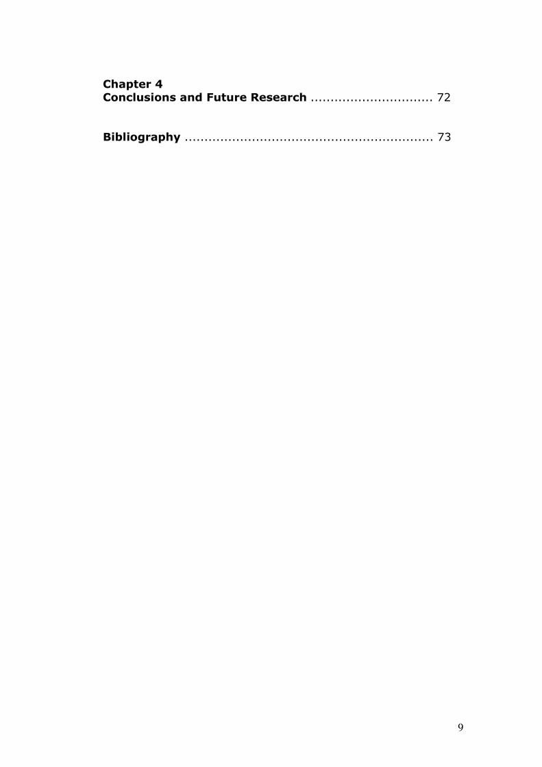
We are going to summarize this process in general lines:
1. DWT Analysis: the dwt is performed to obtainthe multirresolution matrix of wavelet analysiscoefficients from the input signal.
2. Wavelet coefficients matrix split: it is necessaryto split the wavelet analysis coefficients matrixinto vectors of coefficients for each levels. Thisvectors will be used as amplitude factors vectorsin each stream generation for wavelet grainswindowing.
3. Wavelet streams generation: a wavelet stream iscreated for each wavelet level; that is a temporalsuccession of wavelet waveforms windowed byits related wavelet analysis coefficient.
figure 22: Granular synthesis as a additive synthesis of streams
42

4. Wavelet streams addition: the input signal isrecovered from a synchronous sum of differentlevels wavelet streams.
A graphic explanation of this process is shown at thegraphic in the next page:
43
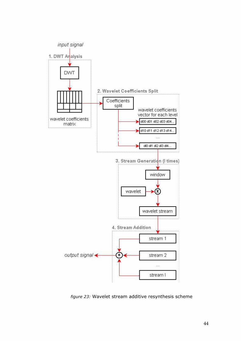
figure 23: Wavelet stream additive resynthesis scheme
44

This implementation of the inverse wavelet transform bymeans of an audio signal processing instead of classicdecimating filter banks or lifting scheme allow us to manipulateaudio directly in the same way we can manipulate audio grainsin granular synthesis. Thus we can recover any sound from itsset of wavelet analysis coefficients, or we can modify thissound by two kind of manipulations: modifications in thewavelet analysis coefficients matrix (data manipulations) or inthe wavelet streams generation (audio manipulations). Bothmodifications can be performed in real time.
Obviously, this implementation means processing a bigamount of data (thousand of ''wavelet grains'') in a microsoundtime scale as well as granular synthesis process a big amountof sound grains.
2.2. PD implementation of a Wavelet Stream AdditiveResynthesis
The pd implementation of the scheme explained in thelast section looks like that:
45

That is the main patch that contains the parametercontrols and all the subpatches which performances thedifferent functions. This implementation allow us to load asound file (*.wav) which is analyzed and recovered in real-time using the wavelet stream additive synthesis scheme. Thisanalysis and resynthesis are performed by blocks of 2048samples because would be impossible to performance theanalysis and resynthesis of the whole sound file. Therefore, thewhole analysis / resynthesis process is performed each block(each 2048 samples). We will know why this value of 2048samples is chosen during the next explanation.
We are going to explain this implementation step bystep:
2.2.1.Initializations
This subpatch contain the initializations we need beforeto start the analysis and resynthesis. Contain another foursubpatches: init, index2level, window_generator andwavelet_generator.
– init: the necessary parameters before theperformance are initialized: sr_khz set the samplerate
figure 24: main patch
46

in kHz, on_bang send a bang to another subpatchesafter this loadbang (due to execution orders), pdcompute audio is switched on by sending 1 to pd dsp,main screen parameters are initialized (gain,wavelet_type, nblocks and duration) and thedwtcoef table is resized to 2048 samples (block size).
– index2level: this subpatch create an index2leveltable which relate the dwt coefficients table indexwhich its related level. Levels are named in that way:
– level 0: coarser average s00 (DC component; 1sample)
– level 1: highest frequency difference dj-1 (1024samples)
– level 2: difference dj-2 (512 samples)– level 3: difference dj-3 (256 samples)– level 4: difference dj-4 (128 samples)– level 5: difference dj-5 (64 samples)– level 6: difference dj-6 (32 samples)– level 7: difference dj-7 (16 samples)– level 8: difference dj-8 (8 samples)– level 9: difference dj-9 (4 samples)– level 10: difference dj-10 (2 samples)– level 11: lowest frequency difference dj-11 (1 sample)
figure 25: init subpatch
47
There areonly 11
levels because of the block size of 2048 samples (log2
(2048) = 11). Each level cover a octave bandfrequency with center frequencies from 22050 Hz atlevel 1 to 21.53 Hz at level 11 (fc = 44100/2level; asamplerate of 44100 Hz is supposed). Levels higherthan level 11 are not necessaries because they coverfrequencies under 20 Hz, so a number of eleven levelsis enough and we can use a block size of 2048samples.
The table index2level stores the level value ofeach index in the way dwt~ external distribute thecoefficients of each level at its output (take a look atfigure 21). This table will be read to obtain the levelnumber from index coefficient number and to store itinto a message together with the coefficient value.
In this implementation a level counter from 0 to11 is triggered using the abstraction until_counter
figure 26: index2level subpatch
48

(faster and more efficient than a classic pd counterscheme because it uses until looping mechanism).For each level another counter is triggered. Thiscounter gives the number of samples of current level(end value). This value is modified by jump and initvalues to obtain the indexes (samples number)related with the current level. A C-like code allow us abetter understanding of this process:
for (i=0; i<12; i++){level = i;init = 2^(i-1);jump = 2^i;end = 2^(11-i); for (j=0; j<end; j++)
{sample = init + (j * jump);}
}
sample is the index value of index2level table andlevel is the level value stored in the table.
– window_generator: this subpatch contain severalwindow abstractions (for different levels). windowabstraction generate a hanning window for a specifiedlevel (stored in table $1_window, where $1 is the levelnumber). The size of the window depend of the levelnumber (size = 7 * 2level). There are only nine windowgenerators, from level 3 to 11. That is due to thenumber of wavelet streams, what will be explained inthe granulator section.
49

– wavelet_generator: this subpatch contain severalwavelet abstractions (for different levels). waveletabstraction generate a wavelet waveform for aspecified level and wavelet type. This waveletwaveform is stored in table $1_wavelet, where $1 isthe level number. In order to generate the wavelettransform we apply the method shown in figure 19,which lie in put an impulse into the idwt. When on_bang is received, an impulse is stored intable $1_impulse, wavelet table is resize in the sameway window table is resized (size = 7 * 2level), and alocal block size (level blocksize) $1_blocksize isgenerated (this block size depend on current level,$1_blocksize = 8 * 2level). After to generate localblock size, $1_impulse is set into idwt to generate$1_wavelet.
figure 27: window abstraction
50

Now, we have generated and initialized all parametersand tables we need (control parameters, index2leveltable, windows tables and wavelets tables) before toload our file and to start the performance
2.2.2.DWT Analysis
This subpatch allow us to load the sound file and to startits dwt analysis.
figure 28: wavelet abstraction
51

Loaded sound file is stored in input table. Then, whenwe press analysis the whole process of analysis / resynthesisstarts. input table is read and sent to dwt~ which stores itsoutput in dwtcoef table. This table is written each 2048samples (equivalent to 0.046 msg if samplerate is 44100). Inorder to achieve this, switch~ object is set to 2048 samplesand overlap of 1 (switch~ object set the processing block size,overlap and down/up-sampling, and allow us to switch DSP onand off). When the sound file reading process has finished,switch~ object is switched off and off_bang value is triggered.
2.2.3.Coefficients list
During the performance this subpatch create a twovalues messages stream. bang~ object trigger theuntil_counter object each 2048 samples (the specified blocksize) when the analysis process starts. This counter count from0 to 2047 at the beginning of each block. The counter act asindex to read index2level and dwtcoef tables. Thus, the leveland coefficient value of each sample is sent in a message atthe output of this subpatch. Therefore, each bang~ time (atthe beginning of each block) 2048 messages with thestructure [level, coefficient value] are sent.
figure 29: dwt_analysis subpatch
52

2.2.4.Granulator
This subpatch contain several stream~ abstractionswhich receive the coefficient messages fromcoefficient_list subpatch and generate the wavelet streamfor each level. This streams are added to the granulatoroutput.
There are nine stream~ abstractions which generate ninewavelet streams from level 3 to 11. First at all, we are going toshow how this abstraction works.
figure 30: coefficients_list subpatch
53
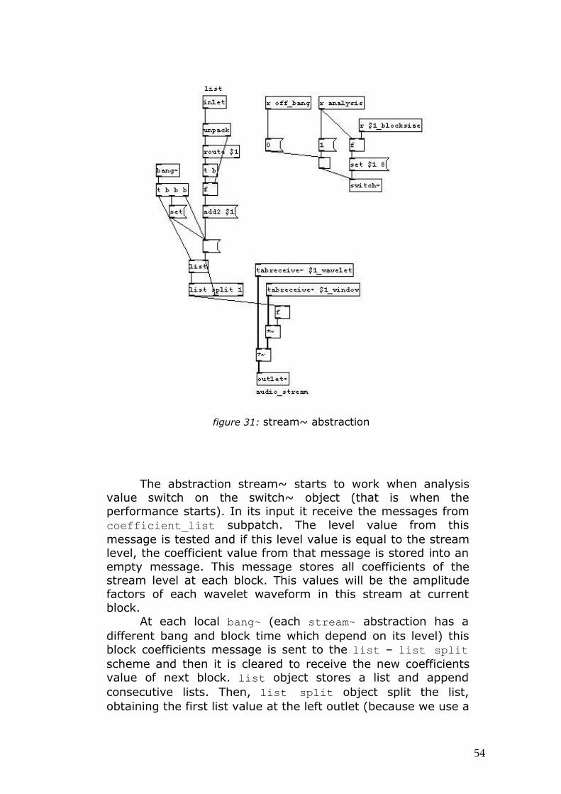
The abstraction stream~ starts to work when analysisvalue switch on the switch~ object (that is when theperformance starts). In its input it receive the messages fromcoefficient_list subpatch. The level value from thismessage is tested and if this level value is equal to the streamlevel, the coefficient value from that message is stored into anempty message. This message stores all coefficients of thestream level at each block. This values will be the amplitudefactors of each wavelet waveform in this stream at currentblock.
At each local bang~ (each stream~ abstraction has adifferent bang and block time which depend on its level) thisblock coefficients message is sent to the list – list splitscheme and then it is cleared to receive the new coefficientsvalue of next block. list object stores a list and appendconsecutive lists. Then, list split object split the list,obtaining the first list value at the left outlet (because we use a
figure 31: stream~ abstraction
54

split point of one) and the remaining ones at the middle outlet.This remaining list is sent again to list object creating adropping mechanism. Each local bang~ a coefficient from theblock coefficients message is sent. This coefficient multiply thecurrent window which multiply the current wavelet, scaling thewavelet waveform based on this analysis coefficient value.
This process is really important because we need aperfect synchronization between the given coefficient and thecurrent performance time and we are working in a microtimescale. Each coefficient must to be related with its correctwavelet. For example, at stream~ abstraction of level three wehave to receive 256 coefficients per block (256 coefficients =blocksize / 2level = 2048 / 23). So we have to trigger acoefficient each 8 samples (2048 / 256 = 8). In order to allowit we use a block size of 64 (8 * 23) with an overlap of 8 whichmeans to obtain a coefficient each 8 samples (23).
In PD block size of 64 samples is the default block size,and the minimum too. It is impossible to process with a blocksize less than 64 samples. That means the previous example(stream~ abstraction of level three) is the highest frequencystream we can generate (5512 Hz). Streams of higherfrequency are impossible to obtain because we need ablocksize less than 64 samples to achieve it.
2.2.5.Output
This subpatch simply send the audio signal we obtain todigital-analog converter in order to listen it.
55

Chapter 3
Audio Manipulations in Wavelet Domain
In this chapter I will explain how we can modify audio inthe wavelet domain with PD.
3.1.Audio Manipulations in Wavelet Domain and its PD Implementation
As we explain in Chapter 1, dwt~ external for PD allowus to obtain a dwt analysis coefficient matrix which we canmodify before to put it into idwt~ external to recover the original sound. Withthis purpose I have implemented a PD patch which allow usdifferent audio manipulations. This is the appearance of itscontrols main screen:
We can see similar controls than the patch shown in the
figure 32: main patch, controls section
56

previous chapter: a load file button, a gain control, a wavelettype selector, duration, nsamples and nblocks information.Moreover we can choose between load a sound file with soundfile button or to use a live signal connected to our input audiodevice (activating live signal toggle). Because of the possibilityof use a live signal a signal level vumeter is added. Clicking onpd modifications box (above load file and live signal buttons)we open another screen which contains all controls for audiomanipulation:
Instead of commenting this audio modifications controlsnow, we are going to explain how this patch works in order toobtain a better understanding of this process. We can take alook at the program section at main patch:
figure 33: modifcations control patch
57

The three subpatches on the up-left corner (pdloadfile, pd live_signal, and pd dwt_analysis) generatethe selected audio input and make its dwt analysis. The twosubpatches under the previous ones (pd dwt_resynthesis,out_volume~) performance the idwt from the modifiedcoefficients list and play the output sound. The threesubpatches on the right (pd list_generator, pdsplit_levels and pd data_modifications) manage the dwtanalysis coefficients and manipulate it in order to modify theinput sound. At the bottom of the screen are the initializationssubptches and the tables which show the input and outputwaveforms.
We are going to explain individually each of this process.
3.1.1.Audio input and dwt analysis
We can choose between to load a sound file (*.wav) orto use a live signal connected to our input audio device (weneed to configure audio settings in pd on order to select theright device).
If we press load_file button we can select a *.wav filewhich is stored in soundfile table (we can take a look at itswaveform by clicking on table soundfile). When we presson_bang this sound file is played and the analysis starts. We
figure 34: main patch, program section
58

can stop this process by clicking on off_bang. We can take alook of this subpatch implementation on next figure:
When we click on live_signal toggle the signal fromadc~ (analog-digital converter object, which obtain the audiosignal from selected input audio device) is sent to thedwt_analysis subpatch instead of the load file signal. Nextfigure show this live_signal subpatch implementation:
figure 35: load_file subpatch
59

Selectedaudio signal (sound file or live signal) is sent to dwt_analysissubpatch which performances the discrete wavelet analysis.Analysis coefficients are stored into dwtcoef table each 2048samples (block size = 2048). We can select which type ofwavelet transform we want (haar, 2nd, 3rd, 4th, 5th or 6th orderinterpolation). on_bang starts the analysis and off_bang stopit. That is the subpatch implementation:
figure 36: live_signal subpatch
figure 37: dwt_analysis subpatch
60

3.1.2.Coefficients manipulations
Wavelet analysis coefficients are stored in dwtcoef tableand we need to manage it and manipulate it in order to obtaindifferent audio modifications.
The first step is to create a message stream with theanalysis coefficient value and its related level and index. This isthe purpose of list_generator subpatch of which implementation is shownon next figure:
Each block_bang (that means at the beginning of eachblock) until_counter abstraction act as index counting from 0to 2047 which allow to read tables index2level and dwtcoef(index2level is created in the same way and with the samepurpose than in previous chapter). This tables provide the level
figure 38: list_generator subpatch
61

and analysis coefficient of each index respectively.index_counter gives an index number from 0 to 2047 eachbang which is modified by pitch value.
This three values are stored in a message with thisorder: [level, index, coefficient]. Each block_bang one of thismessage is sent to the subpatch outlet.
This messages are received by split_levels subpatchwhich route each message depending on its level. From thispoint messages of different levels have an independentlyproces:
This independently process is made by amodification_level abstraction.
figure 39: split_levels subpatch
62

Messages of each level are processed by its relatedmodification_level abstraction. This abstraction modify theanalysis coefficient value which is multiply by the output ofrandomization abstraction (a random number generator withan specified range and frequency of generation) and by a$1_level (a level factor from equalization controls). Thismodified coefficient is put again into a message with its relatedindex.
All modified messages from different levels are sent towrite_coef abstraction which writes again this coefficientsinto a new table call idwtcoef table:
The index which control the writing of coefficients into
figure 40: modification_levelabstraction
figure 41: write_coef abstraction
63
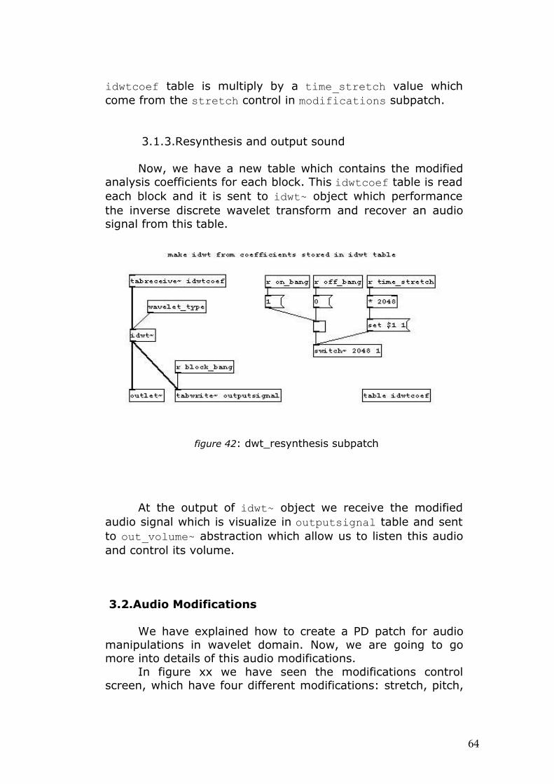
idwtcoef table is multiply by a time_stretch value whichcome from the stretch control in modifications subpatch.
3.1.3.Resynthesis and output sound
Now, we have a new table which contains the modifiedanalysis coefficients for each block. This idwtcoef table is readeach block and it is sent to idwt~ object which performancethe inverse discrete wavelet transform and recover an audiosignal from this table.
At the output of idwt~ object we receive the modifiedaudio signal which is visualize in outputsignal table and sentto out_volume~ abstraction which allow us to listen this audioand control its volume.
3.2.Audio Modifications
We have explained how to create a PD patch for audiomanipulations in wavelet domain. Now, we are going to gomore into details of this audio modifications.
In figure xx we have seen the modifications controlscreen, which have four different modifications: stretch, pitch,
figure 42: dwt_resynthesis subpatch
64

equalization and randomization. We are going to commenteach of this modifications separately.
3.2.1.Stretch
This effect have not to be confused with a time-stretch.The name ''stretch'' for this modification is due to thestretching of the resynthesis block size. The stretch control has5 values: 0.125, 0.25, 0.5, 1 (value by default), 2 and 4. Theselected value multiply the block size in resynthesis process(dwt_resynthesis subpatch). Thus, stretch values higherthan one uses a higher block size in resynthesis process (4096or 8192), while values lower than one uses a smaller block size(1024, 512 or 256). One value keep the same block size thanin analysis process (2048).
The meaning of this modification is a big distortion ofsound frequencial spectrum which consist of low frequenciessuppression in stretch values lower than one and highfrequencies suppression in stretch values higher than one.Moreover, this process generates an apparition of someharmonics in spectrum related with block size. In next figurewe can compare both spectrum of original signal and spectrumof this signal processed with a stretch value of 0.125 (blocksize/ 8):
65

In this figure, red line show original signal spectrum(original signal is a 10 seconds white noise), while blue linerepresent the modified signal spectrum (stretch value =0.125). We can look how the lowest frequencies are reduced inthe modified signal (frequencies lower than 150 Hz), whilesignificant peaks appear at specific points in spectrum (172,344, 516, 689, 861, 1033 and 1205 Hz). The first point at 172Hz is directly related with current block size of 256 samples(2048 / 8): samplerate / blocksize = 44100 / 256 = 172. Thisfirst harmonic is related with a discontinuity each 256 samplesdue to this block size. Successive harmonics are separated 172Hz in a kind of modulation process. The same principle whichcreates this harmonics is perceived as a beating for highstretch values (specially with a value of four). This is due tothe block sizes and its related frequencies (44100 / 4096 =10.7 Hz, and 44100 / 8096 = 5.3 Hz). This frequencies are solow that are perceived as a fast beat instead of a frequencycomponent (this frequencies are below the human perceptionfrequency range).
figure 43: original and modified signals spectrum
66

This process produces a big sound distortion with a kindof pitch shift perception. If we modify a human voice soundwith stretch values higher than 1 we can listen a very deep,low tone voice sound which is intelligible with stretch value of2 but difficultly understandable with value of 4. The samehuman voice sound processed with stretch value lower than 1is unintelligible, higher pitched and scattered.
3.2.2.Shift
As well as the previous modification, this effect must notto be confused with a pitch shift. The shift word is referred to aprocess of analysis coefficient shift. At messages generationprocess, an index value is generated from a counter to relatedthe current coefficient with its time position and frequencylevel. The shift value is added to this index value, in order torelate time-level position of current coefficient with shift value.This value don’t make a simple time shift or pitch shift oncurrent coefficient. Instead of this, the effect of shift valuedepend on its numeric value. If we use an odd shift value, forexample one, all coefficients will be related with next waveletwaveform, which means a big distortion because coefficientC1,0 will envelope wavelet related to coefficient C2,0, coefficientC2,0 will envelope wavelet related to coefficient C1,1, coefficientC1,1 will envelope wavelet related to coefficient C3,0, etc.
If we use an even shift value, for example two, allcoefficients are shifted two positions, which means a time shiftfor level one (because level one is stored in all even samples)and a time and level shift for another levels.
figure 44: shift = 1
67

We can listen how different is the distortion produced byan odd shift value with regard to an even shift value.
3.2.3. Equalization
The equalization controls looks as a typical octave bandgraphic equalizer:
In order to implement this equalizer, wavelet analysis
figure 45: shift = 2
figure 46: equalization controls
68

coefficients for each level are multiplied by its relatedfrequency band gain. Each level cover an octave band with thespecified central frequency. Numeric value of each frequencyband equalization are not dB gain values, instead of that, theyare multiplication values: for example, one value doesn’tamplify its band, two value multiply by two its band gain (+3dBs), and 0.5 value divide by two its band gain (-3 dBs).
3.2.4. Randomization
This effect allow us to randomize audio output with aspecified randomization range and frequency. We can take alook to randomization controls in the next figure:
69

Randomization controls are independent for each level;we can select a different randomization range and frequencyfor different frequency bands, or we can randomize only onefrequency band. Randomization parameters are applied onlywhen we switch on the on/off randomization toggle. If thistoggle is switched off, randomization is not applied. We canreset randomization values by means of clicking on resetbottom. Values by default are 0 for frequency, which could bebetween 0 and 1000 Hz, and 20 for range, which could bebetween 5 and 80.
randomization abstraction is insidemodification_level abstraction. We can take a look to
figure 47: randomization controls
70

randomization abstraction in the next figure:
When random_toggle (on/off toggle) is switched on, arandom generator generate a number between 0 and 1000each 2 msg. This number is evaluated with moses functiondepending on the current frequency value ($1_freq). Onlyrandom numbers lower than current frequency value are putat the left outlet of moses function. That means the higher thefrequency value, the higher the frequency of random numbersgeneration. This random numbers set a bang for anothernumber generator between 0 and randomization range value($1_range). The random number we obtain is scaled to set itin a desired range to multiply it by the current waveletanalysis coefficient. Thus, we can apply a randomization ofwavelet analysis coefficients which means an audiorandomization for each level or frequency band.
figure 48: randomization abstraction
71

Chapter 4
Conclusions and Future Research
This work have tried to create a new kind of audioresynthesis by means of additive wavelet streams. The resultof this resynthesis process has not been suitable in its PDimplementation, due to its limitation to generate highfrequency wavelet streams. This lost of high frequencies(above 5 KHz) doesn’t allow us to obtain an original signalperfect reconstruction. Because of this, audio manipulation inthis analysis-resynthesis process have not been implemented.Future researches could try to achieve a perfect signal
reconstruction by means of this wavelet additive streamresynthesis with a different implementation. Maybe animplementation of this scheme on a DSP could offer betterresults. The idea and theory of this wavelet analysis – additivewavelet stream resynthesis process have been presented hereto allow a future deeper research on its possibilities in audiomodification and as a different approach to granular synthesis,which could be focused in computer music purposes.
Possibilities of audio manipulations by means of waveletanalysis – resynthesis with Pure Data have been shown inorder to expand the audio processing tools with PD. Wavelettransform and audio processing in wavelet domain have notbeen used frequently in PD, although that could be a powerfuland interesting tool for audio processing. I hope this workencourages more people to approach wavelet processing withPD.
72

BIBLIOGRAPHY
Books:
– Boulanger, R. (ed.). The Csound Book : Perspectives inSoftware Synthesis, Sound Design, Signal Processing, andProgramming. Cambridge, Massachusetts: The MIT Press,2000.
– Daubechies, I. Ten Lectures on Wavelets. SIAM, 1992.
– Daubechies, I. & Sweldens, W. Factoring WaveletTransforms Into Lifting Steps, 1996.
– De Poli, G., Piccialli, A. & Roads, C. (ed.). Representations ofMusical Signals. The MIT Press, 1991.
– Dodge, C., & T. Jerse. Computer Music. 2D rev. New York:Schirmer Books, 1997.
– Don, G. W. & Walker, J. S. Time-Frequency Analysis ofMusic, 2005.
– Heinz Gerhards, R. Sound Analysis, modification, andResynthesis with Wavelet Packets. University of BritishColumbia, 1986.
– Holzapfel, M., Hoffmann, R. & Höge, H. A Wavelet-DomainPSOLA Approach. Institute for Technical Acoustics, TechnicalUniversity of Dresden.
– Hoskinson, R. Manipulation and Resynthesis ofEnvironmental Sounds with Natural Wavelet Grains. McGillUniversity, 1996.
– Keller, D. & Truax, B. Ecologically-based granularsynthesis. School for the Contemporary Arts, Simon FraserUniversity.
73

– Kussmaul. C. Applications of Wavelets in Music. The WaveletFunction Library. Darmouth College, Hanover, NewHampshire, 1991.
– Miner, N. E. & Caudell, T. P. Using Wavelets to SynthesizeStochastic-based Sounds for Immersive VirtualEnvironments. University of New Mexico.
– Misiti, M., Misiti, Y., Oppenheim, G., Poggi, J. M. WaveletToolbox. User's Guide, version 2. The MathWorks, Inc. 2000.
– Opie, T. T. Creation of a Real-Time Granular SynthesisInstrument for Live Performance. Queensland University ofTechnology, 2003
– Oppenheim, A. V. & Schaffer, R. W. Digital SignalProcessing. Prentice-Hill, 1975.
– Puckette, M. Theory and Techniques of Electronic Music.University of California, 2005.
– Reck Mirand, E. (ed.). Computer sound design: synthesistechniques and programming. Focal Press, 2002.
– Rowe, R. Machine Musicianship. The MIT Press, 2001.
– Sarkar, T. K., Su, C., Adve, R., Salazar-Palma, M., Garcia-Castillo, L. & Boix, R. R. A Tutorial on Wavelets from anElectrical Engineering Perspective. 1.Discrete WaveletTechniques. IEEE Antennas and Propagation Magazine, Vol.40, No.5. 1998.
– Serrano, E. P. Introducción a la transformada wavelet y susaplicaciones al procesamiento de señales de emisiónacústica. Escuela de Ciencia y Tecnología, UniversidadNacional de General San Martín.
– Schnell, N. GRAINY - Granularsynthese in Echzeit. B.E.M. 4,Intitut für Elektronische Musik, Graz, 1995.
– Sweldens, W. & Schröder, P. Building Your Own Wavelets atHome.
– Torrence, C. & Compo, G. P. A Practical Guide to WaveletAnalysis. University of Colorado.
– Wornell, G. Signal Processing with Fractals: A Wavelet-
74

Based Approach. MIT, Prentice Hall. 1996.
– Xiang, P. A new Scheme for Real-Time Loop MusicProduction Based on Granular Similarity and ProbabilityControl. DAFx02, 2002.
– Zölzer, U. (ed.). DAFX - Digital Audio Effects. John Wiley &Sons, 2002.
Web Sites:
– PD Portal: puredata.org
– The PD-List Archives: lists.puredata.info/pipermail/pd-list
– The Wavelet Digest: www.wavelet.org
– The Wavelet Tutorial:users.rowan.edu/~polikar/WAVELETS/WTtutorial.html
– Wikipedia: wikipedia.org
75