Complex-valued wavelet lifting and

applications

Jean HamiltonHEDS, ScHARR, University of Sheffield

Matthew A. Nunes∗

Department of Mathematics and Statistics, Lancaster University

Marina I. KnightDepartment of Mathematics, University of York

andPiotr Fryzlewicz

Department of Statistics, London School of Economics

January 10, 2017

Abstract

Signals with irregular sampling structures arise naturally in many fields. In applica-tions such as spectral decomposition and nonparametric regression, classical methodsoften assume a regular sampling pattern, thus cannot be applied without prior dataprocessing. This work proposes new complex-valued analysis techniques based on thewavelet lifting scheme that removes ‘one coefficient at a time’. Our proposed liftingtransform can be applied directly to irregularly sampled data and is able to adapt to thesignal(s)’ characteristics. As our new lifting scheme produces complex-valued waveletcoefficients, it provides an alternative to the Fourier transform for irregular designs,allowing phase or directional information to be represented. We discuss applications inbivariate time series analysis, where the complex-valued lifting construction allows forcoherence and phase quantification. We also demonstrate the potential of this flexiblemethodology over real-valued analysis in the nonparametric regression context.

Keywords: lifting scheme; wavelets; nondecimated transform; (bivariate) time series; coher-ence and phase; nonparametric regression.

∗Corresponding author: m.nunes@lancaster.ac.uk

1

1 Introduction

Since the early nineties, wavelets have become a popular tool for nonparametric regression,

statistical image processing and time series analysis. In particular, due to their natural

localisation, wavelets can provide sparse representations for certain functions that cannot be

represented efficiently using Fourier sinusoids. Reviews of the use of wavelets in statistics

include Nason (2008) and Abramovich et al. (2000).

Until recently, the majority of work in the statistical literature has been based on the

discrete wavelet transform (DWT). However, classical wavelet methods suffer from some

limitations; in particular, usage is restricted to data sampled at regular time or spatial loca-

tions, and a dyadic data dimension is often imposed. Wavelet lifting (Sweldens, 1996) can be

used to overcome many of the shortcomings of the standard DWT. Specifically, wavelet func-

tions obtained through the wavelet lifting scheme provide an extension of classical wavelet

methods to more general settings, such as irregularly sampled data.

On the other hand, it is now well-established that complex-valued data analysis tools

can extract useful information that is potentially missed when using traditional real-valued

wavelet techniques, even for real-valued data, see for example Lina and Mayrand (1995); Fer-

nandes et al. (2003); Selesnick et al. (2005). In particular, using complex-valued multiscale

methods has been advantageous in a range of statistical applications such as nonparamet-

ric regression (Barber and Nason, 2004), image processing (Kingsbury, 1999; Portilla and

Simoncelli, 2000) and time series analysis (Magarey and Kingsbury, 1998; Kingsbury, 2001).

Complex-valued multiscale techniques building upon the lifting scheme as introduced by

Sweldens (1996) have been introduced in the literature by Abbas and Tran (2006), who

briefly investigated their proposed technique in the image denoising context, and by Shui

et al. (2003), who focused on the design of complex filters with desired band-pass properties.

This article introduces a new adaptive complex-valued wavelet lifting scheme built upon

the lifting ‘one coefficient at a time’ (LOCAAT) framework of Jansen et al. (2001, 2009).

A nondecimated variant of the proposed transform, which allows for an overcomplete repre-

sentation of such data is also introduced. The added benefits of our methodology are: (i)

flexibility – it can be applied to irregularly sampled grids of (possibly) non-dyadic length;

(ii) information augmentation – through the complex-valued wavelet coefficients, the scheme

2

exploits additional signal information not used by real-valued transforms; and (iii) applica-

bility – it allows for the analysis of bivariate nonstationary signals with possibly different

(irregular) sampling structures, previously not directly possible using methods currently in

the literature.

We demonstrate the benefits of our new technique for spectral estimation of irregularly

sampled time series, with a particular focus on coherence and phase quantification for irreg-

ularly sampled bivariate time series. In this context, the methodology can be viewed as a

wavelet lifting analogue to the Fourier transform and can be used for the same purposes. The

good performance of our method is also displayed in the nonparametric regression setting.

The paper is organised as follows. Section 2 introduces the new complex-valued lift-

ing algorithm, including its overcomplete variant. Section 3 details the application of the

complex-valued lifting algorithm to discover local frequency content of irregularly sampled

uni- and bivariate time series. Section 4 tackles nonparametric regression for (real-valued)

signals.

2 The complex-valued lifting scheme

The lifting scheme (Sweldens, 1996) was introduced as a flexible way of providing wavelet-

like transforms for irregular data. Lifting bases are naturally compactly supported, and via

the recursive nature of the transform, one can build wavelets with desired properties, such as

vanishing moments. In addition, lifting algorithms are known to be computationally faster

than traditional wavelet transforms since they require fewer computations compared with

classical transforms. For an overview of the lifting scheme, see Schroder and Sweldens (1996)

or Jansen and Oonincx (2005).

In this section we introduce a complex-valued lifting scheme for analysing irregularly

sampled signals. The proposed lifting scheme can be thought of as a wavelet lifting analogue

to the Fourier transform. An irregularly sampled signal is decomposed into a set of complex-

valued wavelet (or detail) coefficients, representing the variation in the data as a function of

location and wavelet scale (comparable to Fourier frequency).

In a nutshell, the scheme can be conceptualised in two branches: one branch of the trans-

form provides the real-valued part of the detail coefficient and the second branch represents

3

the imaginary component. Hence by using two different (real-valued) lifting schemes, one

obtains a complex-valued decomposition, akin to the dual-tree complex wavelet transform

of Kingsbury (2001). However, our approach differs from that of Kingsbury (2001) in that

it employs two lifting schemes linked through orthogonal prediction filters, rather than two

separate DWTs. The new scheme is therefore able to extract information from signals via

the two filters whilst also naturally coping with the irregularity of the observations. Our

approach also differs fundamentally from the complex-valued lifting techniques currently in

the literature (Abbas and Tran, 2006; Shui et al., 2003) through the particular filter con-

struction we propose (Section 2.2) in conjunction with the lifting construction that removes

‘one coefficient at a time’ (Section 2.1). This allows us to embed adaptivity in our complex-

valued multiscale setup, i.e. construct wavelet functions whose smoothness adjusts to the

local properties of the signal.

In what follows we introduce the proposed scheme using an abstract choice of real and

imaginary filters, and the subject of filter choice is deferred until Section 2.2, while an

overcomplete version of the complex-valued lifting transform is introduced in Section 2.3.

2.1 The algorithm

Suppose a function f(· ) is observed at a set of n irregularly spaced locations, x = (x1, . . . , xn).

The proposed lifting scheme aims to decompose the data collected over the irregularly sam-

pled grid, {(xi, fi = f(xi))}ni=1, into a set of R smooth coefficients and (n−R) complex-valued

detail coefficients, with R the desired resolution level. The quantity R is akin to the primary

resolution level in classical wavelet transforms, see Hall and Patil (1996) for more details.

We propose to construct a new complex-valued transform that builds upon the LOCAAT

paradigm of Jansen et al. (2001, 2009), shown to efficiently represent local signal features

in the fields of nonparametric regression (Nunes et al., 2006; Knight and Nason, 2009) and

spectral estimation (Knight et al., 2012). We shall therefore refer to our proposed algorithm

under the acronym C-LOCAAT.

Similar to the real-valued LOCAAT algorithm, C-LOCAAT can be described by recur-

sively applying three steps: split, predict and update, which we detail below. At the first

stage (n) of the algorithm, the smooth coefficients are set as cn,k = fk, the set of indices of

smooth coefficients is Sn = {1, . . . , n} and the set of indices of detail coefficients is Dn = ∅.

4

The (irregular) sampling is described using the distance between neighbouring observations,

and at stage n we define the span of xk as sn,k = xk+1−xk−1

2. The sampling irregularity is

intrinsically linked to the notion of wavelet scale, which in this context becomes continuous,

as opposed to dyadic in the classical wavelet settings; this results in each coefficient having

an associated scale across a continuum. This aspect will be discussed in detail following the

introduction of the C-LOCAAT algorithm.

In the split step, a point jn to be lifted is chosen. Typically, points from the densest

sampled regions are removed first, but other predefined removal choices are also possible

(see Section 2.3). We shall often refer to the removal order as a trajectory.

In the predict step the set of neighbours (Jn) of the point jn are identified and used

to estimate the value of the function at the selected point jn. In contrast to real-valued

LOCAAT algorithms, this is achieved using two prediction schemes, each defined by its

respective filters, L and M. The filter L corresponds to estimation via regression over the

neighbourhood, as is usual in LOCAAT. In order to extract further information from the

signal, our proposal is to construct the second filter (M) orthogonal on L, to ensure that it

exploits further local signal information to the filter L. Section 2.2 discusses this in detail.

The prediction residuals from using the two filters are given by

λjn = lnjncn,jn −∑

i∈Jn

lni cn,i, (1)

µjn = mnjncn,jn −

∑

i∈Jn

mni cn,i, (2)

where {lni }i∈Jn∪{jn} and {mni }i∈Jn∪{jn} are the prediction weights associated with L and M.

The complex-valued detail (wavelet) coefficient we propose is obtained by combining the

two prediction residuals

djn = λjn + iµjn. (3)

In the update step, the smooth coefficients {cn,i}i∈Jn and spans of the neighbours {sn,i}i∈Jn

are updated according to filter L:

cn−1,i = cn,i + bni λjn,

sn−1,i = sn,i + lni sn,jn ∀i ∈ Jn, (4)

where bni are update weights. In practice, the update weights are chosen such that the mean

of the series is preserved throughout the transform, thus preserving the characteristics of the

5

original series (Jansen et al., 2009). One such choice is to set bni = (sn,jnsn−1,i)/(∑

i∈Jn s2n−1,i).

The neighbours’ spans update accounts for the modification to the sampling grid induced by

removing one of the observations. Updating according to the L filter only ensures that there

is a unique coarsening of the signal for both the real and imaginary parts of the transform.

The observation jn is then removed from the set of smooth coefficients, hence after the

first algorithm iteration, the index set of smooth and detail coefficients are Sn−1 = Sn\{jn}

and Dn−1 = {jn} respectively. The algorithm is then iterated until the desired primary

resolution level R has been achieved. In practice, the choice of the primary level R in

LOCAAT lifting schemes is not crucial provided it is sufficiently low (Jansen et al., 2009),

with R = 2 recommended by Nunes et al. (2006).

After observations jn, jn−1, . . . , jR+1 have been removed, the function can be represented

as a set of R smooth coefficients, {cr−1,i}i∈SR, and (n−R) detail coefficients, {dk}k∈DR

(DR =

{jn, ..., jR+1}). As in classical wavelet decompositions, the detail coefficients represent the

high frequency components of f(· ), whilst the smooth coefficients capture the low frequency

content in the data.

The lifting scheme can be easily inverted by recursively ‘undoing’ the update, predict and

split steps described above for the first filter. Specifically, the update step is first inverted:

cn,i = cn−1,i − bni λjn, ∀i ∈ Jn, then the predict step is inverted by

cn,jn =λjn −

∑

i∈Jn lni cn,i

lnjnor (5)

cn,jn =µjn −

∑

i∈Jn mni cn,i

mnjn

. (6)

Undoing either predict (5) or (6) step is sufficient for inversion. As for real-valued lift-

ing, inversion can also be performed via matrix calculations due to the transform linearity.

However, using (5) for inversion is generally computationally faster, especially for large n.

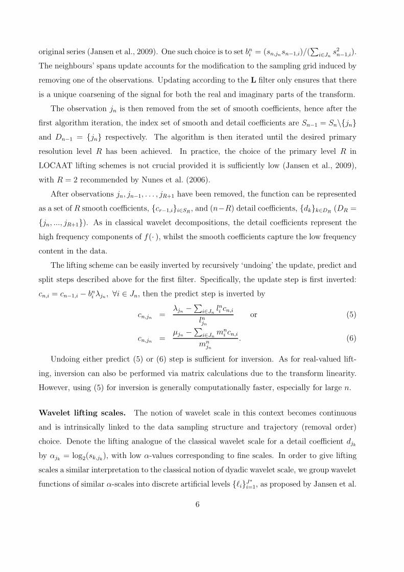
Wavelet lifting scales. The notion of wavelet scale in this context becomes continuous

and is intrinsically linked to the data sampling structure and trajectory (removal order)

choice. Denote the lifting analogue of the classical wavelet scale for a detail coefficient djk

by αjk = log2(sk,jk), with low α-values corresponding to fine scales. In order to give lifting

scales a similar interpretation to the classical notion of dyadic wavelet scale, we group wavelet

functions of similar α-scales into discrete artificial levels {ℓi}J∗

i=1, as proposed by Jansen et al.

6

(2009), for a chosen J∗. The further use of artificial scales is discussed in Sections 2.3 and

3 (under the spectral estimation context) and in Appendix B (under the nonparametric

regression context). Note that the usage of the same lifting trajectory for the two lifting

branches (coupled with the one filter update) ensures that our proposed lifting transform

generates a common scale for both real and imaginary parts. In other words, at each stage of

the algorithm there is just one set of smooth coefficients associated to a unique set of scales.

>

...

>

>

>

>

>

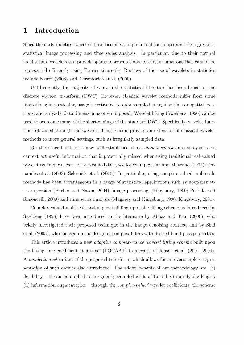
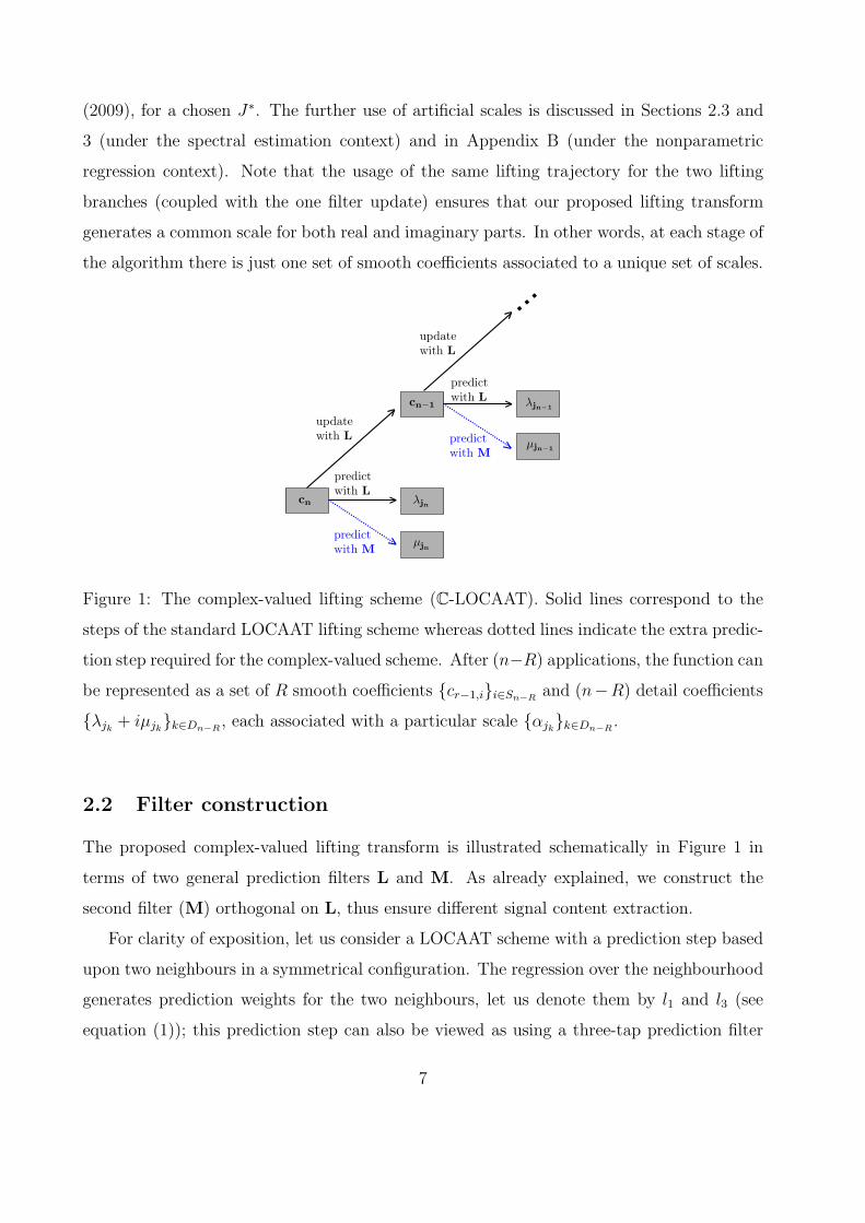
Figure 1: The complex-valued lifting scheme (C-LOCAAT). Solid lines correspond to the

steps of the standard LOCAAT lifting scheme whereas dotted lines indicate the extra predic-

tion step required for the complex-valued scheme. After (n−R) applications, the function can

be represented as a set of R smooth coefficients {cr−1,i}i∈Sn−Rand (n−R) detail coefficients

{λjk + iµjk}k∈Dn−R, each associated with a particular scale {αjk}k∈Dn−R

.

2.2 Filter construction

The proposed complex-valued lifting transform is illustrated schematically in Figure 1 in

terms of two general prediction filters L and M. As already explained, we construct the

second filter (M) orthogonal on L, thus ensure different signal content extraction.

For clarity of exposition, let us consider a LOCAAT scheme with a prediction step based

upon two neighbours in a symmetrical configuration. The regression over the neighbourhood

generates prediction weights for the two neighbours, let us denote them by l1 and l3 (see

equation (1)); this prediction step can also be viewed as using a three-tap prediction filter

7

(L) of the form (l1, 1, l3), which depends on the sampling of the observations x = (x1, . . . , xn)

(Nunes et al., 2006). We determine the unique (up to proportionality) three-tap filter M

that is orthogonal on L and ensures at least one vanishing moment. Hence we can express

the set of filter pairs as having the form

L = (l1, 1, l3), l1, l3 > 0

M = (m1, m2, m3),

and l1m1 + m2 + l3m3 = 0 (i.e. L · M = 0) and l1 + l3 = 1, m1 + m3 = m2 (i.e. ensure

one vanishing moment). The solution to these constraints can be parameterised as M =

(−1+l31+l1

m, l1−l31+l1

m,m). The proportionality constant can be determined by bringing both

filters L and M to the same scale through ‖L‖ = ‖M‖, which yields m = l1+1√3. Hence the

solution can be succinctly written as M = (Am, (1 + A)m,m) with A = l1−2l1+1

and m = l1+1√3.

This particular example of the lead filter L represents a prediction scheme using linear

regression with two neighbours in a symmetrical configuration. This is a choice that has

proved to be successful both for (real-valued) nonparametric regression (Nunes et al., 2006;

Knight and Nason, 2009) and for (real-valued) spectral estimation (Knight et al., 2012).

Since L can be viewed as a prediction filter for a real-valued LOCAAT scheme, we

can also employ the adaptive prediction filter choice of Nunes et al. (2006) in our proposed

construction. The ‘best’ local regression (order and neighbourhood) is chosen at each predict

step, subject to yielding minimising the detail coefficients. Consequently, we obtain an

adaptive complex-valued lifting transform, with the highly desirable flexibility of being able

to adapt to the local characteristics of the data – see Appendix B in the supplementary

material for an illustration of this adaptiveness in the nonparametric regression setting.

The orthogonality of the two filters M and L also mirrors the attractive properties of

Fourier sinusoids, hence this choice results in an interpretable quantification of phase, which

shall further be exploited according to the context—by phase alteration when denoising

real-valued signals, or by ensuring phase preservation in the context of spectral estimation.

A further insight and justification of the proposed filter choice is provided in Appendix

C in the context of coherence and phase estimation.

8

2.3 The nondecimated complex-valued lifting transform

In the classical wavelet literature, the nondecimated wavelet transform (NDWT) (Nason

and Silverman, 1995) has properties that make it a better choice than the discrete wavelet

transform (DWT) for certain classes of problems, see e.g. Percival and Walden (2006). The

concept is akin to basis averaging, and has delivered successful results in both nonpara-

metric regression and spectral estimation problems, not only in the classical wavelet setting

(NDWT) but also for irregularly spaced data through the nondecimated lifting transform

(NLT) (Knight and Nason, 2009; Knight et al., 2012).

In this section, we also exploit the benefits of this nondecimation paradigm for irregularly

sampled data and to this end, we shall introduce the complex-valued nondecimated lifting

transform (CNLT). However, note that our use of the term ’nondecimation’ differs from the

classical NDWT. Specifically, due to the irregular sampling structure, nondecimation cannot

be performed via decomposing shifts of input data without data interpolation.

Although similar in spirit to the NLT, our transform hinges on the proposed complex-

valued lifting scheme (Section 2.1) and therefore yields an overcomplete complex-valued data

representation, extracting additional signal information. In particular, the CNLT algorithm

results in a wavelet transform that yields (complex-valued) wavelet coefficients at each grid

point (x) and at multiple scales (α).

Next we shall describe our proposed univariate and bivariate CNLT techniques. We shall

show that in the nonparametric regression setting, our univariate proposal significantly out-

performs current wavelet and non-wavelet denoising techniques (see Section 4 and Appendix

B), while its bivariate extension allows for estimation of the dependence between pairs of

series (see Section 3).

2.3.1 Univariate CNLT

So far, the proposed complex-valued lifting scheme decomposes the original signal {(xi, fi =

f(xi))}ni=1 into a set of R smooth coefficients and (n−R) complex detail (wavelet) coefficients,

with each detail coefficient djk corresponding to exactly one scale αjk .

We now aim to construct a new scheme that transforms the original signal into a collection

of smooth and detail coefficients, with each x-location associated to a collection of several

9

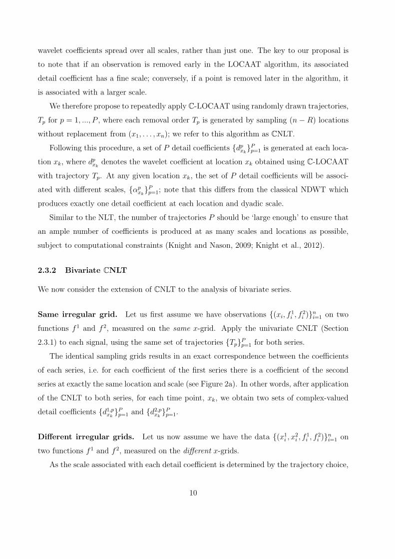
wavelet coefficients spread over all scales, rather than just one. The key to our proposal is

to note that if an observation is removed early in the LOCAAT algorithm, its associated

detail coefficient has a fine scale; conversely, if a point is removed later in the algorithm, it

is associated with a larger scale.

We therefore propose to repeatedly apply C-LOCAAT using randomly drawn trajectories,

Tp for p = 1, ..., P , where each removal order Tp is generated by sampling (n− R) locations

without replacement from (x1, . . . , xn); we refer to this algorithm as CNLT.

Following this procedure, a set of P detail coefficients {dpxk}Pp=1 is generated at each loca-

tion xk, where dpxkdenotes the wavelet coefficient at location xk obtained using C-LOCAAT

with trajectory Tp. At any given location xk, the set of P detail coefficients will be associ-

ated with different scales, {αpxk}Pp=1; note that this differs from the classical NDWT which

produces exactly one detail coefficient at each location and dyadic scale.

Similar to the NLT, the number of trajectories P should be ‘large enough’ to ensure that

an ample number of coefficients is produced at as many scales and locations as possible,

subject to computational constraints (Knight and Nason, 2009; Knight et al., 2012).

2.3.2 Bivariate CNLT

We now consider the extension of CNLT to the analysis of bivariate series.

Same irregular grid. Let us first assume we have observations {(xi, f1i , f

2i )}

ni=1 on two

functions f 1 and f 2, measured on the same x-grid. Apply the univariate CNLT (Section

2.3.1) to each signal, using the same set of trajectories {Tp}Pp=1 for both series.

The identical sampling grids results in an exact correspondence between the coefficients

of each series, i.e. for each coefficient of the first series there is a coefficient of the second

series at exactly the same location and scale (see Figure 2a). In other words, after application

of the CNLT to both series, for each time point, xk, we obtain two sets of complex-valued

detail coefficients {d1,pxk}Pp=1 and {d2,pxk

}Pp=1.

Different irregular grids. Let us now assume we have the data {(x1i , x

2i , f

1i , f

2i )}

ni=1 on

two functions f 1 and f 2, measured on the different x-grids.

As the scale associated with each detail coefficient is determined by the trajectory choice,

10

time

sca

le

d1

a)

time

sca

le

d2

time

sca

le

x1 x2 x3 x4 x5 x6

b)

time

sca

le

I1, 2

l 1l 2

x1 x2 x3 x4 x5 x6

c)

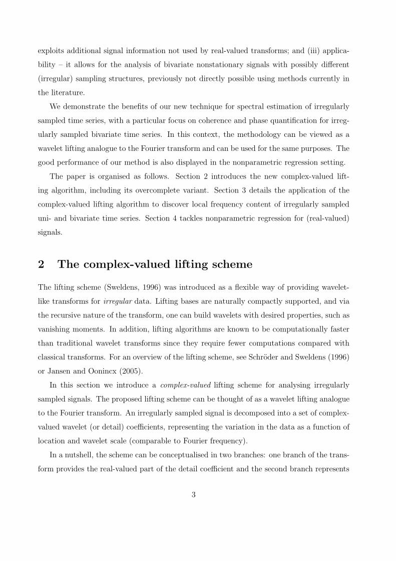
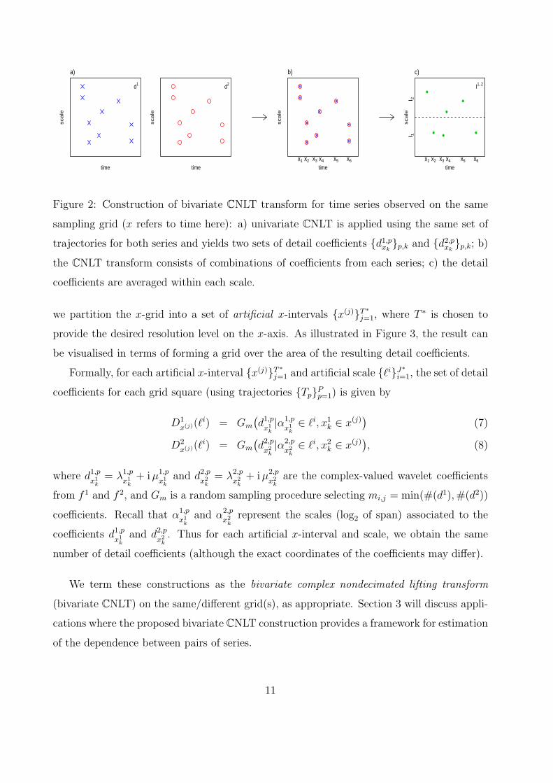
Figure 2: Construction of bivariate CNLT transform for time series observed on the same

sampling grid (x refers to time here): a) univariate CNLT is applied using the same set of

trajectories for both series and yields two sets of detail coefficients {d1,pxk}p,k and {d2,pxk

}p,k; b)

the CNLT transform consists of combinations of coefficients from each series; c) the detail

coefficients are averaged within each scale.

we partition the x-grid into a set of artificial x-intervals {x(j)}T∗

j=1, where T ∗ is chosen to

provide the desired resolution level on the x-axis. As illustrated in Figure 3, the result can

be visualised in terms of forming a grid over the area of the resulting detail coefficients.

Formally, for each artificial x-interval {x(j)}T∗

j=1 and artificial scale {ℓi}J∗

i=1, the set of detail

coefficients for each grid square (using trajectories {Tp}Pp=1) is given by

D1x(j)(ℓ

i) = Gm

(

d1,px1k

|α1,p

x1k

∈ ℓi, x1k ∈ x(j)

)

(7)

D2x(j)(ℓ

i) = Gm

(

d2,px2k

|α2,p

x2k

∈ ℓi, x2k ∈ x(j)

)

, (8)

where d1,px1k

= λ1,p

x1k

+ iµ1,p

x1k

and d2,px2k

= λ2,p

x2k

+ iµ2,p

x2k

are the complex-valued wavelet coefficients

from f 1 and f 2, and Gm is a random sampling procedure selecting mi,j = min(#(d1),#(d2))

coefficients. Recall that α1,p

x1k

and α2,p

x2k

represent the scales (log2 of span) associated to the

coefficients d1,px1k

and d2,px2k

. Thus for each artificial x-interval and scale, we obtain the same

number of detail coefficients (although the exact coordinates of the coefficients may differ).

We term these constructions as the bivariate complex nondecimated lifting transform

(bivariate CNLT) on the same/different grid(s), as appropriate. Section 3 will discuss appli-

cations where the proposed bivariate CNLT construction provides a framework for estimation

of the dependence between pairs of series.

11

time

scale

a)

d1

time

scale

d2

time

scale

b)

D1

time

scale

D2

time

scale

c)

I1, 2

l 1l 2

t1 t2

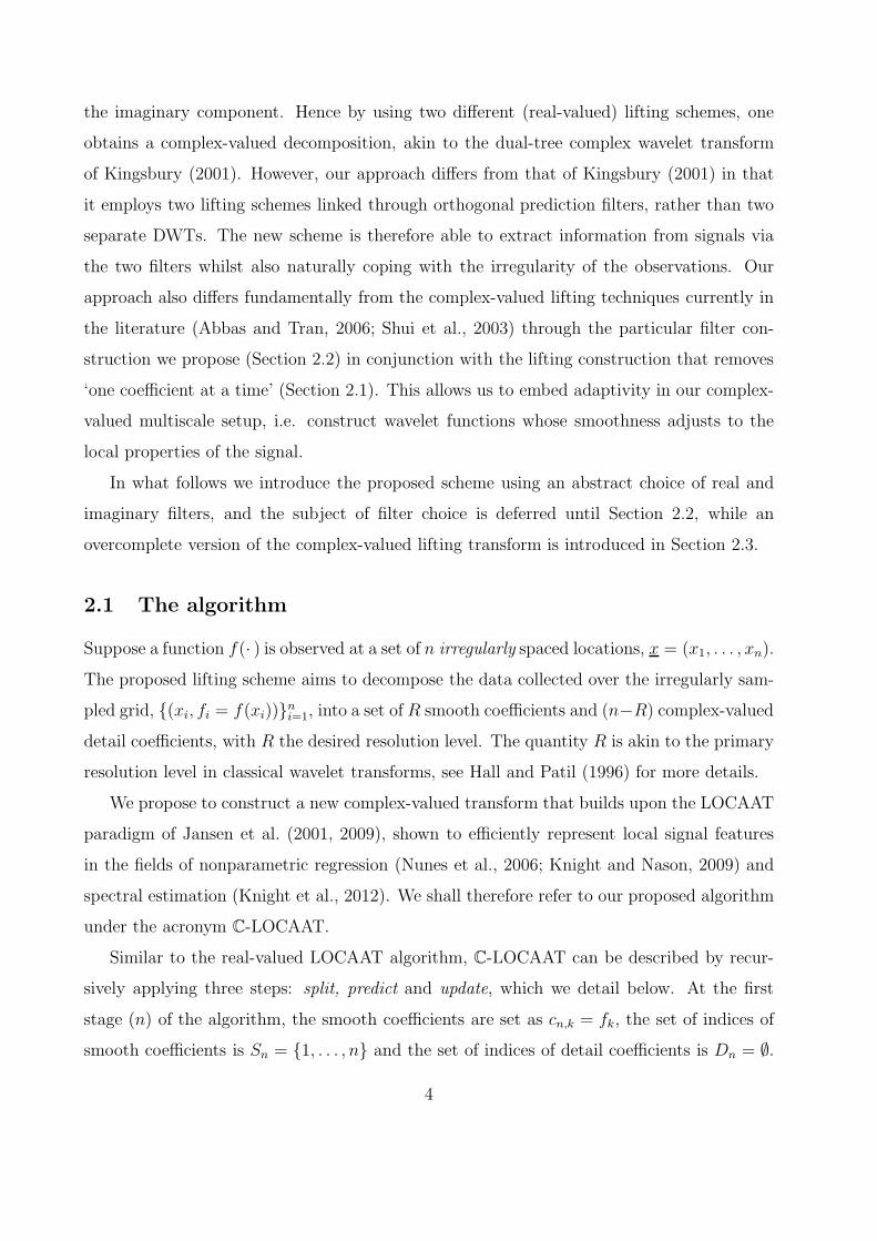
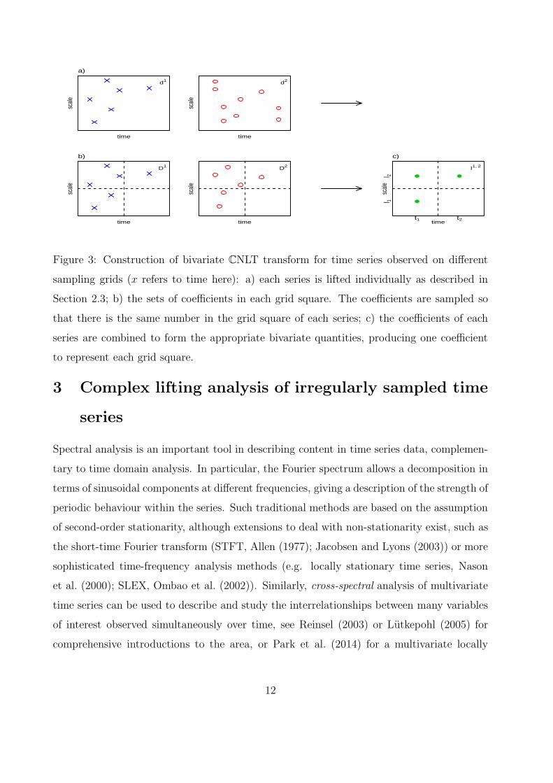
Figure 3: Construction of bivariate CNLT transform for time series observed on different

sampling grids (x refers to time here): a) each series is lifted individually as described in

Section 2.3; b) the sets of coefficients in each grid square. The coefficients are sampled so

that there is the same number in the grid square of each series; c) the coefficients of each

series are combined to form the appropriate bivariate quantities, producing one coefficient

to represent each grid square.

3 Complex lifting analysis of irregularly sampled time

series

Spectral analysis is an important tool in describing content in time series data, complemen-

tary to time domain analysis. In particular, the Fourier spectrum allows a decomposition in

terms of sinusoidal components at different frequencies, giving a description of the strength of

periodic behaviour within the series. Such traditional methods are based on the assumption

of second-order stationarity, although extensions to deal with non-stationarity exist, such as

the short-time Fourier transform (STFT, Allen (1977); Jacobsen and Lyons (2003)) or more

sophisticated time-frequency analysis methods (e.g. locally stationary time series, Nason

et al. (2000); SLEX, Ombao et al. (2002)). Similarly, cross-spectral analysis of multivariate

time series can be used to describe and study the interrelationships between many variables

of interest observed simultaneously over time, see Reinsel (2003) or Lutkepohl (2005) for

comprehensive introductions to the area, or Park et al. (2014) for a multivariate locally

12

stationary wavelet approach.

This work aims to deal with a further additional challenge, that of irregular sampling.

Irregularly sampled time series arise in many scientific applications, e.g. finance (Engle,

2000; Gencay et al., 2001), astronomy (Bos et al., 2002; Broerson, 2008) and environmental

science (Witt and Schumann, 2005; Wolff, 2005) to name just a few. Many applications deal

with the sampling irregularity either by means of a time-frequency Lomb-Scargle approach

under the assumption of time series stationarity (Vanıcek, 1971; Lomb, 1976; Scargle, 1982),

or process the data prior to analysis, restoring it to a regular grid then suitable for analysis

by standard methods, see for example Erdogan et al. (2004) or Broerson (2008). Although

it is convenient to work within a regularly spaced time series setting, a typical result will

amount to signal smoothing, leading to information loss at high frequencies and estimation

bias (Frick et al., 1998; Rehfeld et al., 2011).

Many time series observed in practice will exhibit (second-order) nonstationary behaviour

as well as being irregularly sampled. Although the literature does currently offer (albeit

few) options for the analysis of irregularly sampled nonstationary series (see e.g. Foster

(1996); Frick et al. (1998); Knight et al. (2012)), there is no well established method for

estimating the dependence between pairs of such signals. In the next section, we propose to

describe the local frequency content of irregularly sampled time series by making use of the

proposed complex-valued lifting scheme and introducing a complex-valued cross-periodogram

and associated measures.

3.1 The complex lifting periodogram

Recall that the CNLT provides a set of detail coefficients and associated scales {dpxk, αp

xk}Pp=1,

where the scale associated with each detail coefficient αpxk

is a continuous quantity. In a spirit

similar to that of Knight et al. (2012), this information will allow a time-scale decomposition

(typically termed the (wavelet) periodogram) of the variability in the data, with the crucial

difference that the wavelets coefficients are now complex-valued and therefore contain more

information. In constructing the periodogram, we use a set of discrete artificial scales,

{ℓi}J∗

i=1, which partitions the range of the continuous lifting scales {αpxk} for all p and k, with

J∗ chosen to provide a desired periodogram ‘granularity’. Each scale αpxk

will fall into one

unique level ℓi for each p and observation xk; let Pi,k = {p : αpxk

∈ ℓi} denote the set of

13

trajectories such that xk is associated with a scale in the set ℓi, and ni,k = |Pi,k| denote the

size of the set. For each time point xk, k = 1, . . . , n and artificial scale ℓi, i = 1, . . . , J∗, we

introduce the complex lifting periodogram (also referred to in text as CNLT periodogram)

Ixk(ℓi) =

1

ni,k

∑

p∈Pi,k

|dpxk|2 =

1

ni,k

∑

p∈Pi,k

(λpxk)2 +

1

ni,k

∑

p∈Pi,k

(µpxk)2,

where | · | denotes the complex modulus.

3.2 The complex lifting cross-periodogram

Similar to other complex wavelet transforms (Portilla and Simoncelli, 2000; Selesnick et al.,

2005), the complex-valued nature of the bivariate CNLT coefficients (see Section 2.3.2) pro-

vides both local phase and spectral information. In order to estimate the dependence between

pairs of time series, we first define the complex lifting cross-periodogram, the cross-spectral

analogue of the periodogram. As in Section 2.3.2, our discussion will be split based on

whether the data has been sampled over the same or different grids.

Bivariate time series observed on the same grid. For each time point xk, k = 1, . . . , n

and artificial scale ℓi, i = 1, . . . , J∗, define the complex lifting cross-periodogram (also re-

ferred to as CNLT cross-periodogram) for series observed on the same grid as

I(1,2)xk(ℓi) =

1

ni,k

∑

p∈Pi,k

d1,pxkd2,pxk

, (9)

where d1,pxk= λ1,p

xk+ iµ1,p

xkand d2,pxk

= λ2,pxk

+ iµ2,pxk

are the detail coefficients from f 1 and f 2.

The CNLT cross-periodogram consists of combinations of coefficients from each series and

provides information about the relationship between the signals. Note that unlike the CNLT

periodogram, the cross-periodogram is complex-valued.

Similar to classical Fourier cross-spectrum methodology (see e.g. Priestley (1983)), the

CNLT cross-periodogram can be separated into its real and imaginary parts to define the

CNLT co-periodogram and the CNLT quadrature periodogram, respectively resulting in

cxk(ℓi) =

1

ni,k

∑

p∈Pi,k

λ1,pxkλ2,pxk

+1

ni,k

∑

p∈Pi,k

µ1,pxkµ2,pxk,

qxk(ℓi) =

1

ni,k

∑

p∈Pi,k

µ1,pxkλ2,pxk

−1

ni,k

∑

p∈Pi,k

λ1,pxkµ2,pxk.

14

These quantities, together with the individual lifting spectra of each process, can be used to

calculate the measures of phase and coherence between the two series f 1 and f 2:

φxk(ℓi) = tan−1

(−qxk(ℓi)

cxk(ℓi)

)

, (10)

ρxk(ℓi) =

√

cxk(ℓi)2 + qxk

(ℓi)2√

I(1)xk

(ℓi)I(2)xk

(ℓi)

. (11)

The CNLT cross-periodogram provides a measure of the dependence between series, but its

magnitude is affected by the individual CNLT periodograms of the signals. Hence as in the

regularly sampled setting, it is preferable to normalise this quantity, providing a coherence

measure that satisfies 0 ≤ ρxk(ℓi) ≤ 1 (as in (11)). This is similar to the coherence measure

for regularly sampled signals introduced in Sanderson et al. (2010). The CNLT phase as

defined in (10) provides an indication of any time lag between the signals. Several examples

examining the coherence and phase between signal pairs are given in Section 3.3.

Bivariate time series observed on different grids. Closer to real data scenarios, we

now consider time series that were sampled over different irregular grids, with one such

real data example being discussed in Section 3.3.3. In order to obtain the cross-spectral

quantities, we combine the appropriate sets of detail coefficients for each grid, corresponding

to f 1 and f 2, i.e. D1x(j)(ℓ

i) and D2x(j)(ℓ

i) introduced in equations (7) and (8). For each

artificial time period, x(j), j = 1, . . . , T ∗ and artificial scale ℓi, i = 1, . . . , J∗, we define the

complex lifting cross-periodogram for series observed on different irregular grids as

I(1,2)

x(j) (ℓi) =

1

ni,j

ni,j∑

s=1

order{D1x(j)(ℓ

i)}s order{D2x(j)(ℓi)}s, (12)

where ni,j is the number of pairs in the grid square defined at time x(j) and scale ℓi, and

order{D}s indicates the sth time-ordered detail.

If the sampling schemes coincide for the two series ({x1k}k ≡ {x2

k}k) and the same tra-

jectories are used to generate the details {d1,pxk}p,k, respectively {d2,pxk

}p,k, then equations (9)

and (12) coincide, except for the quantities being also averaged over the defined artificial

time period. The co- and quadrature periodograms may be obtained in the same fashion as

above, and subsequently used to yield the lifting phase and coherence in this setting.

15

Figures 2 and 3 provide a visual representation for the complex lifting cross-periodogram

construction under the assumption of the same, respectively different sampling grids.

We now make some remarks about the proposed periodogram constructions.

Scale interpretation. The relationship between artificial scale (ℓi) and classical Fourier

frequency can be described in terms of the scale which maximises the coherence for a Fourier

wave of period T . Defining ρ(ℓi) = 1n

∑n

k=1 ρxk(ℓi), the design of the filters outlined in Section

2.2 is such that ℓi = argmaxj∈{1,...,J∗} ρ(ℓj) = T/3.

We emphasise that this relationship is dictated by the choice of filter pairs: the CNLT

periodogram and co-periodogram (as defined above) are composed of the sum of the wavelet

coefficients from the two schemes, while the quadrature periodogram contains products of the

coefficients. Hence to ensure that the resulting estimates are interpretable, the two filters are

specified so that combinations of coefficients (either through multiplication or summation)

provide the same scale-frequency relationship (see Sanderson (2010), Sections 5.3 and 6.2.1).

The provided mapping between wavelet lifting scale and Fourier frequency can be used to

compare our results to those of classical Fourier-based methods (see Section 3.3 next).

Periodogram smoothing over time. As is customary, the CNLT periodogram will be

smoothed over time using simple moving average smoothing, i.e. we compute Ixk(ℓi) =

1

#(M ik)

∑

j∈M ikIxj

(ℓi), where M ik = {j : xk −M i < xj ≤ xk +M i} and M i denotes the width

of the averaging window, permitted to take different values for each scale, li.

3.3 Examples

We now illustrate the proposed methodology by application to both simulated and real

irregular time series. The results were produced in the R statistical computing environment

(R Core Team, 2013), using modifications to the code from the adlift package (Nunes and

Knight, 2012) and the nlt package (Knight and Nunes, 2012).

3.3.1 Simulated data

Signals sampled on the same irregular sampling grid. In this example, the meth-

ods of Section 3.2 are applied to bivariate series observed on the same sampling grid:

16

{(xk, f1k , f

2k )}

200k=1, where

f 1k = sin

(

2πxk

10

)

+ sin

(

2πxk

30

)

+ sin

(

2πxk

70

)

+ ζ1k ,

f 2k = sin

(

2π(xk − τ)

30

)

+ ζ2k ,

where τ = 0 for xk < 200 and τ = 6 for xk ≥ 200, and the quantities ζ1k and ζ2k are

independent, identically distributed Gaussian variables with mean zero and variance 0.22.

The observations are irregularly sampled such that (xk+1−xk) ∈ {n/10 : n = 10, 11, . . . , 30}

and 1(n−1)

∑n−1k=1(xk+1 − xk) = 2.

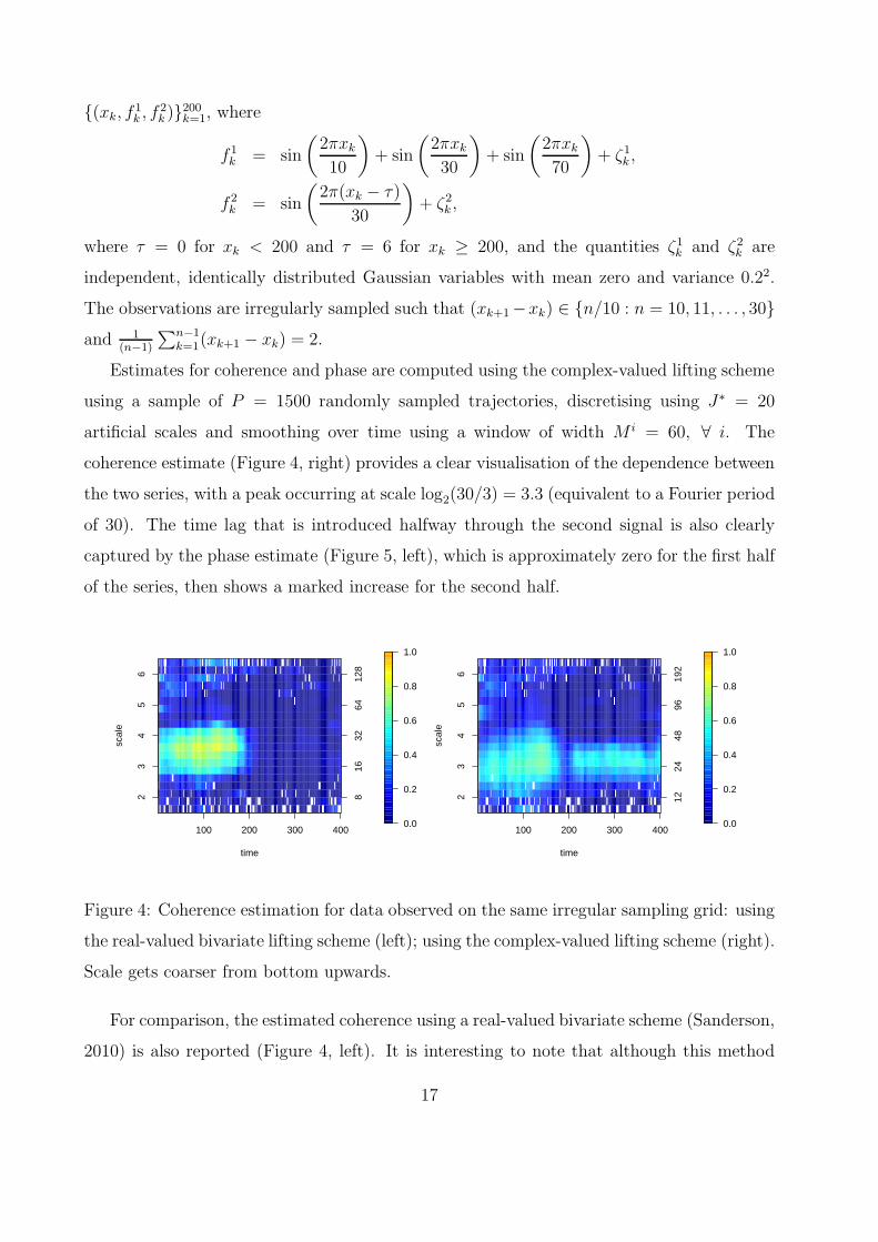
Estimates for coherence and phase are computed using the complex-valued lifting scheme

using a sample of P = 1500 randomly sampled trajectories, discretising using J∗ = 20

artificial scales and smoothing over time using a window of width M i = 60, ∀ i. The

coherence estimate (Figure 4, right) provides a clear visualisation of the dependence between

the two series, with a peak occurring at scale log2(30/3) = 3.3 (equivalent to a Fourier period

of 30). The time lag that is introduced halfway through the second signal is also clearly

captured by the phase estimate (Figure 5, left), which is approximately zero for the first half

of the series, then shows a marked increase for the second half.

time

scal

e

100 200 300 400

23

45

6

816

3264

128

0.0

0.2

0.4

0.6

0.8

1.0

time

scal

e

100 200 300 400

23

45

6

1224

4896

192

0.0

0.2

0.4

0.6

0.8

1.0

Figure 4: Coherence estimation for data observed on the same irregular sampling grid: using

the real-valued bivariate lifting scheme (left); using the complex-valued lifting scheme (right).

Scale gets coarser from bottom upwards.

For comparison, the estimated coherence using a real-valued bivariate scheme (Sanderson,

2010) is also reported (Figure 4, left). It is interesting to note that although this method

17

time

scal

e

100 200 300 400

23

45

6

1224

4896

192

−1.5

−1.0

−0.5

0.0

0.5

1.0

1.5

time

scal

e

100 200 300 400

23

45

6

1224

4896

192

−1.5

−1.0

−0.5

0.0

0.5

1.0

1.5

time

scal

e

0 100 200 300 400

23

45

6

1224

4896

192

−1.5

−1.0

−0.5

0.0

0.5

1.0

1.5

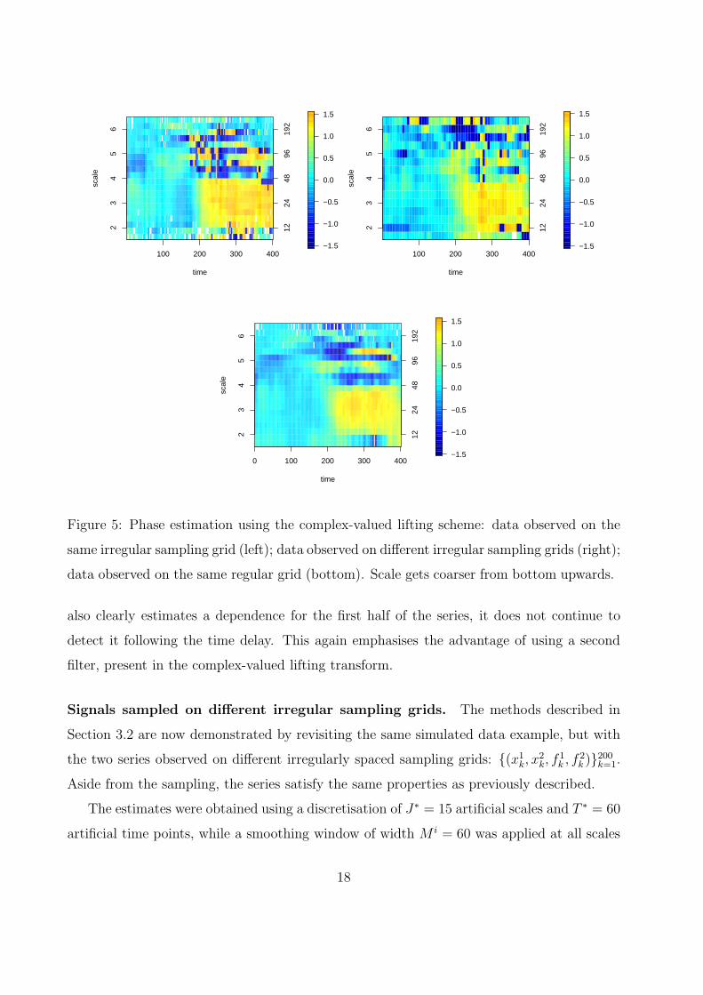
Figure 5: Phase estimation using the complex-valued lifting scheme: data observed on the

same irregular sampling grid (left); data observed on different irregular sampling grids (right);

data observed on the same regular grid (bottom). Scale gets coarser from bottom upwards.

also clearly estimates a dependence for the first half of the series, it does not continue to

detect it following the time delay. This again emphasises the advantage of using a second

filter, present in the complex-valued lifting transform.

Signals sampled on different irregular sampling grids. The methods described in

Section 3.2 are now demonstrated by revisiting the same simulated data example, but with

the two series observed on different irregularly spaced sampling grids: {(x1k, x

2k, f

1k , f

2k )}

200k=1.

Aside from the sampling, the series satisfy the same properties as previously described.

The estimates were obtained using a discretisation of J∗ = 15 artificial scales and T ∗ = 60

artificial time points, while a smoothing window of width M i = 60 was applied at all scales

18

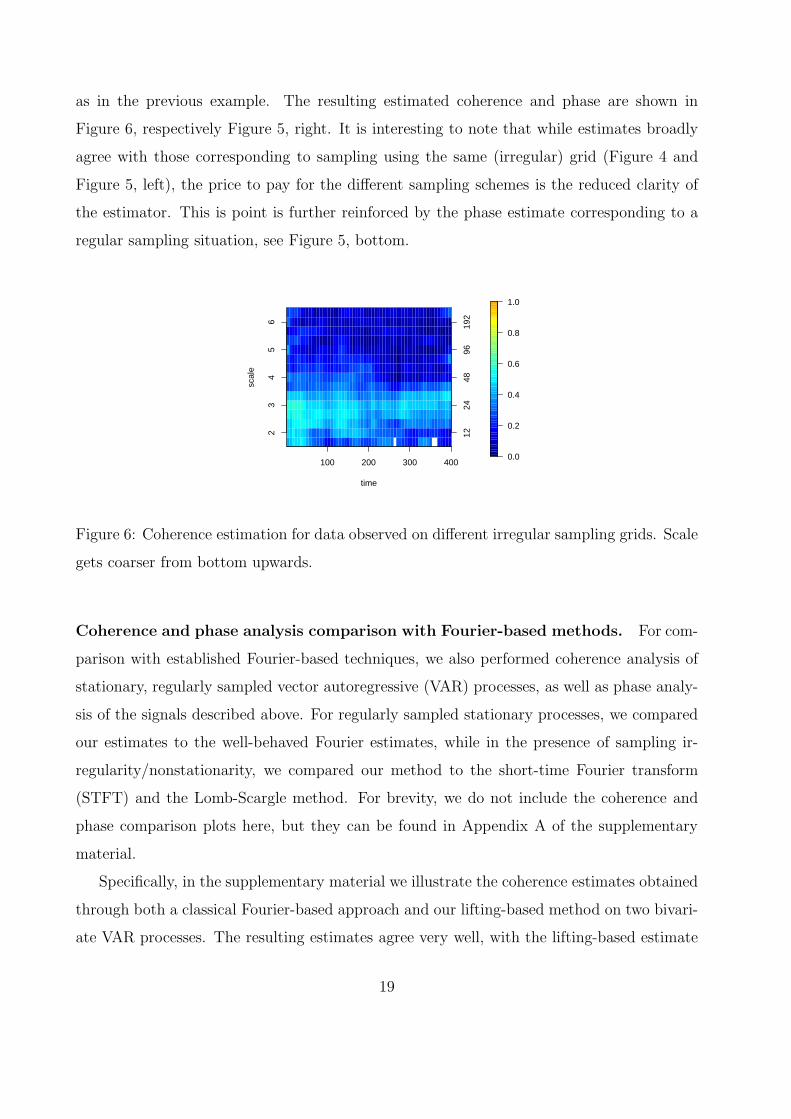
as in the previous example. The resulting estimated coherence and phase are shown in

Figure 6, respectively Figure 5, right. It is interesting to note that while estimates broadly

agree with those corresponding to sampling using the same (irregular) grid (Figure 4 and

Figure 5, left), the price to pay for the different sampling schemes is the reduced clarity of

the estimator. This is point is further reinforced by the phase estimate corresponding to a

regular sampling situation, see Figure 5, bottom.

time

scal

e

100 200 300 400

23

45

6

1224

4896

192

0.0

0.2

0.4

0.6

0.8

1.0

Figure 6: Coherence estimation for data observed on different irregular sampling grids. Scale

gets coarser from bottom upwards.

Coherence and phase analysis comparison with Fourier-based methods. For com-

parison with established Fourier-based techniques, we also performed coherence analysis of

stationary, regularly sampled vector autoregressive (VAR) processes, as well as phase analy-

sis of the signals described above. For regularly sampled stationary processes, we compared

our estimates to the well-behaved Fourier estimates, while in the presence of sampling ir-

regularity/nonstationarity, we compared our method to the short-time Fourier transform

(STFT) and the Lomb-Scargle method. For brevity, we do not include the coherence and

phase comparison plots here, but they can be found in Appendix A of the supplementary

material.

Specifically, in the supplementary material we illustrate the coherence estimates obtained

through both a classical Fourier-based approach and our lifting-based method on two bivari-

ate VAR processes. The resulting estimates agree very well, with the lifting-based estimate

19

displaying a slight depreciation when compared to the well-behaved Fourier estimates, suited

for regular sampling and stationary process behaviour. However, in general if the data is

believed to be amenable to be analysed with standard methodology, Fourier-based estima-

tion should be preferred to the proposed method which was specifically designed to offer a

solution for the challenging situations that include irregular sampling.

As already highlighted, traditional methods do not readily handle data that feature both

potential nonstationarities and irregular sampling, thus STFT required further intervention

while the Lomb-Scargle method failed to account for nonstationarity. Thus in order to obtain

the desired phase analysis, we mapped the irregular data to a regular grid (by e.g. interpo-

lation) and then used STFT in order to capture the nonstationary time-frequency content of

the data. The Lomb-Scargle analysis naturally dealt with the sampling irregularity, but as-

sumed stationarity and therefore it did not provide time-localisation information. The phase

estimation plots of the STFT method exhibit little resolution in time or frequency, possibly

due to the spectral blurring induced by the overlapping windows in the STFT as noted in

Shumway and Stoffer (2013). Furthermore, for signals sampled over different irregular grids,

the method creates additional blurring in the phase plot. By contrast, the Lomb-Scargle

method is able to deal naturally with the irregular sampling structure of the signals, but it

does not contain any time-phase information. In addition, there is no marked distinction in

frequency where the phase is large, unlike for that of our complex lifting method (see Figure

5). These features yet again highlight the appeal of our technique.

3.3.2 Simulated data with varying time delay

The next example explores the effect of increasing the time delay between two signals. For

each value of τ = 1, . . . , 15, the series {(xk, f1k , f

2k )}

200k=1 are simulated following

f 1k = sin

(

2πxk

30

)

+ ζ1k ,

f 2k = sin

(

2π(xk − τ)

30

)

+ ζ2k ,

where (xk+1 − xk) ∈ {n/10 : n = 10, 11, . . . , 30} and 1(n−1)

∑n−1k=1(xk+1 − xk) = 2, ζ1k and ζ2k

are independent, identically distributed Gaussian variables with mean zero, variance 0.22.

Just as in the classical (Fourier) analysis, it is interesting to inspect the coherence and

phase across frequencies (here, scales) in order to relate the common behaviour of the two

20

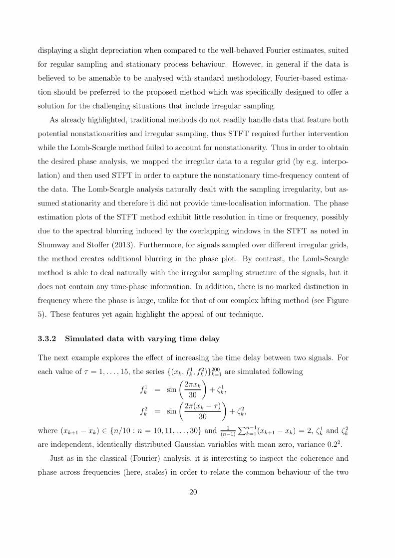
series and possible time delays, respectively. The estimated coherence and phase correspond-

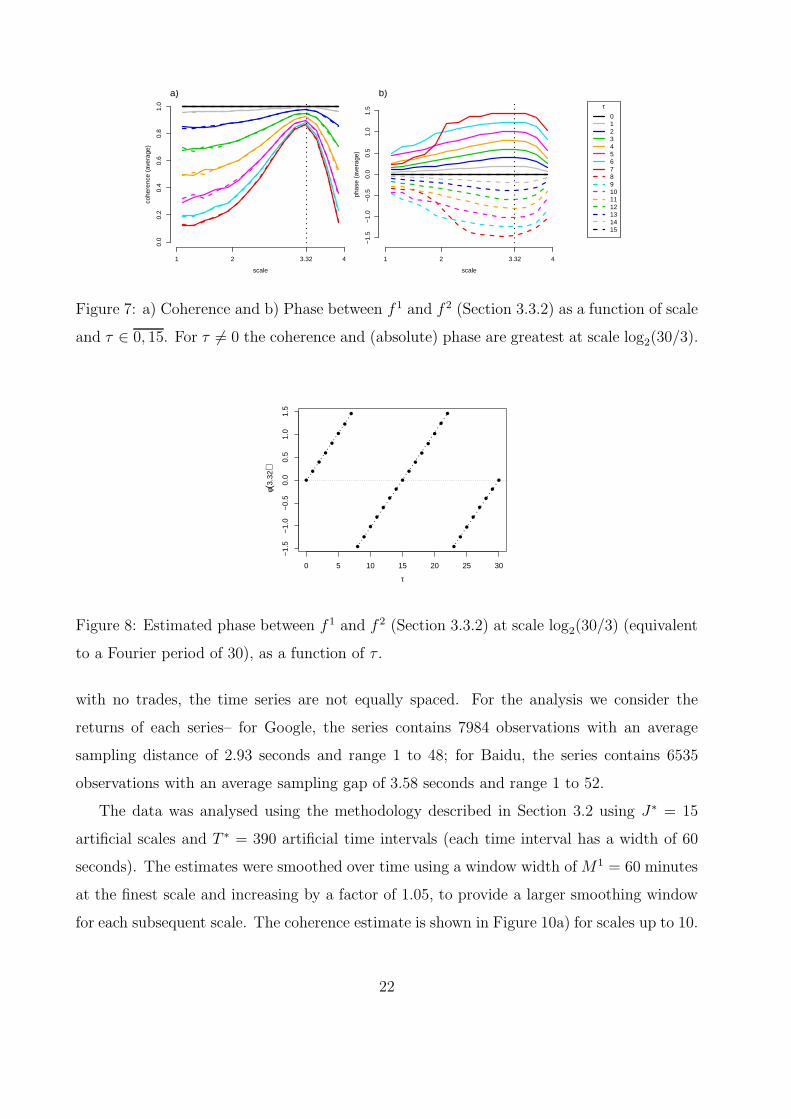
ing to the increasing τ = 1, . . . , 15 are shown in Figure 7. To give an overall sense of the

coherence and phase magnitude over time, the estimates are averaged over the full time

range to give ρ(ℓi) = 1200

∑200k=1 ρxk

(ℓi). We used P = 750 randomly sampled trajectories and

discretised using J∗ = 20 artificial scales.

When τ = 0, the coherence is 1 and the phase is 0. For τ 6= 0 the coherence is greatest

at a scale of log2(30/3), corresponding to the period of variation (T = 30) in the data. The

coherence intensity and response over scale are affected by the magnitude of the time delay.

The coherence is lowest at time delays around 7.5 (T/4), and at these shifts the peak at scale

log2(30/3) is also more pronounced. At τ = 15 (T/2) the signals are sign reversed versions

of each other and, again, the observed coherence is 1 at all scales. The phase is also greatest

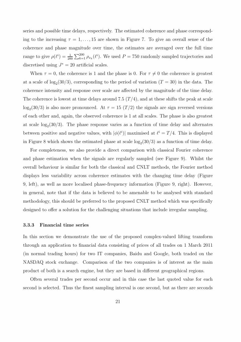
at scale log2(30/3). The phase response varies as a function of time delay and alternates

between positive and negative values, with |φ(ℓi)| maximised at ℓi = T/4. This is displayed

in Figure 8 which shows the estimated phase at scale log2(30/3) as a function of time delay.

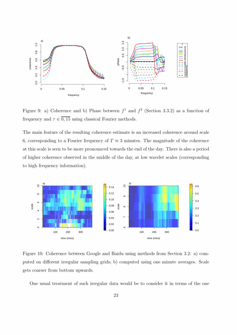
For completeness, we also provide a direct comparison with classical Fourier coherence

and phase estimation when the signals are regularly sampled (see Figure 9). Whilst the

overall behaviour is similar for both the classical and CNLT methods, the Fourier method

displays less variability across coherence estimates with the changing time delay (Figure

9, left), as well as more localised phase-frequency information (Figure 9, right). However,

in general, note that if the data is believed to be amenable to be analysed with standard

methodology, this should be preferred to the proposed CNLT method which was specifically

designed to offer a solution for the challenging situations that include irregular sampling.

3.3.3 Financial time series

In this section we demonstrate the use of the proposed complex-valued lifting transform

through an application to financial data consisting of prices of all trades on 1 March 2011

(in normal trading hours) for two IT companies, Baidu and Google, both traded on the

NASDAQ stock exchange. Comparison of the two companies is of interest as the main

product of both is a search engine, but they are based in different geographical regions.

Often several trades per second occur and in this case the last quoted value for each

second is selected. Thus the finest sampling interval is one second, but as there are seconds

21

scale

cohe

renc

e (a

vera

ge)

0.0

0.2

0.4

0.6

0.8

1.0

1 2 3.32 4

a)

scale

phas

e (a

vera

ge)

−1.

5−

1.0

−0.

50.

00.

51.

01.

5

1 2 3.32 4

b)τ

0123456789101112131415

Figure 7: a) Coherence and b) Phase between f 1 and f 2 (Section 3.3.2) as a function of scale

and τ ∈ 0, 15. For τ 6= 0 the coherence and (absolute) phase are greatest at scale log2(30/3).

0 5 10 15 20 25 30

−1.

5−

1.0

−0.

50.

00.

51.

01.

5

τ

φ(3.

32)

Figure 8: Estimated phase between f 1 and f 2 (Section 3.3.2) at scale log2(30/3) (equivalent

to a Fourier period of 30), as a function of τ .

with no trades, the time series are not equally spaced. For the analysis we consider the

returns of each series– for Google, the series contains 7984 observations with an average

sampling distance of 2.93 seconds and range 1 to 48; for Baidu, the series contains 6535

observations with an average sampling gap of 3.58 seconds and range 1 to 52.

The data was analysed using the methodology described in Section 3.2 using J∗ = 15

artificial scales and T ∗ = 390 artificial time intervals (each time interval has a width of 60

seconds). The estimates were smoothed over time using a window width of M1 = 60 minutes

at the finest scale and increasing by a factor of 1.05, to provide a larger smoothing window

for each subsequent scale. The coherence estimate is shown in Figure 10a) for scales up to 10.

22

frequency

cohe

renc

e

0.0

0.2

0.4

0.6

0.8

1.0

0 0.05 0.1 0.15

a)

frequency

phas

e

−1.

5−

0.5

0.5

1.0

1.5

0 0.05 0.1 0.15

b)

τ0123456789101112131415

Figure 9: a) Coherence and b) Phase between f 1 and f 2 (Section 3.3.2) as a function of

frequency and τ ∈ 0, 15 using classical Fourier methods.

The main feature of the resulting coherence estimate is an increased coherence around scale

6, corresponding to a Fourier frequency of T ≈ 3 minutes. The magnitude of the coherence

at this scale is seen to be more pronounced towards the end of the day. There is also a period

of higher coherence observed in the middle of the day, at low wavelet scales (corresponding

to high frequency information).

time (mins)

scal

e

100 200 300

02

46

810

a)

0.00

0.02

0.04

0.06

0.08

0.10

0.12

0.14

time (mins)

scal

e

100 200 300

67

89

10

b)

0.0

0.1

0.2

0.3

0.4

0.5

0.6

Figure 10: Coherence between Google and Baidu using methods from Section 3.2: a) com-

puted on different irregular sampling grids; b) computed using one minute averages. Scale

gets coarser from bottom upwards.

One usual treatment of such irregular data would be to consider it in terms of the one

23

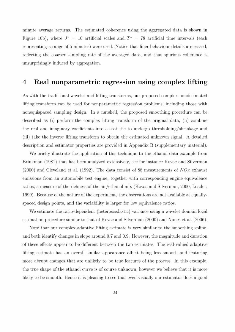
minute average returns. The estimated coherence using the aggregated data is shown in

Figure 10b), where J∗ = 10 artificial scales and T ∗ = 78 artificial time intervals (each

representing a range of 5 minutes) were used. Notice that finer behaviour details are erased,

reflecting the coarser sampling rate of the averaged data, and that spurious coherence is

unsurprisingly induced by aggregation.

4 Real nonparametric regression using complex lifting

As with the traditional wavelet and lifting transforms, our proposed complex nondecimated

lifting transform can be used for nonparametric regression problems, including those with

nonequispaced sampling design. In a nutshell, the proposed smoothing procedure can be

described as (i) perform the complex lifting transform of the original data, (ii) combine

the real and imaginary coefficients into a statistic to undergo thresholding/shrinkage and

(iii) take the inverse lifting transform to obtain the estimated unknown signal. A detailed

description and estimator properties are provided in Appendix B (supplementary material).

We briefly illustrate the application of this technique to the ethanol data example from

Brinkman (1981) that has been analyzed extensively, see for instance Kovac and Silverman

(2000) and Cleveland et al. (1992). The data consist of 88 measurements of NOx exhaust

emissions from an automobile test engine, together with corresponding engine equivalence

ratios, a measure of the richness of the air/ethanol mix (Kovac and Silverman, 2000; Loader,

1999). Because of the nature of the experiment, the observations are not available at equally-

spaced design points, and the variability is larger for low equivalence ratios.

We estimate the ratio-dependent (heteroscedastic) variance using a wavelet domain local

estimation procedure similar to that of Kovac and Silverman (2000) and Nunes et al. (2006).

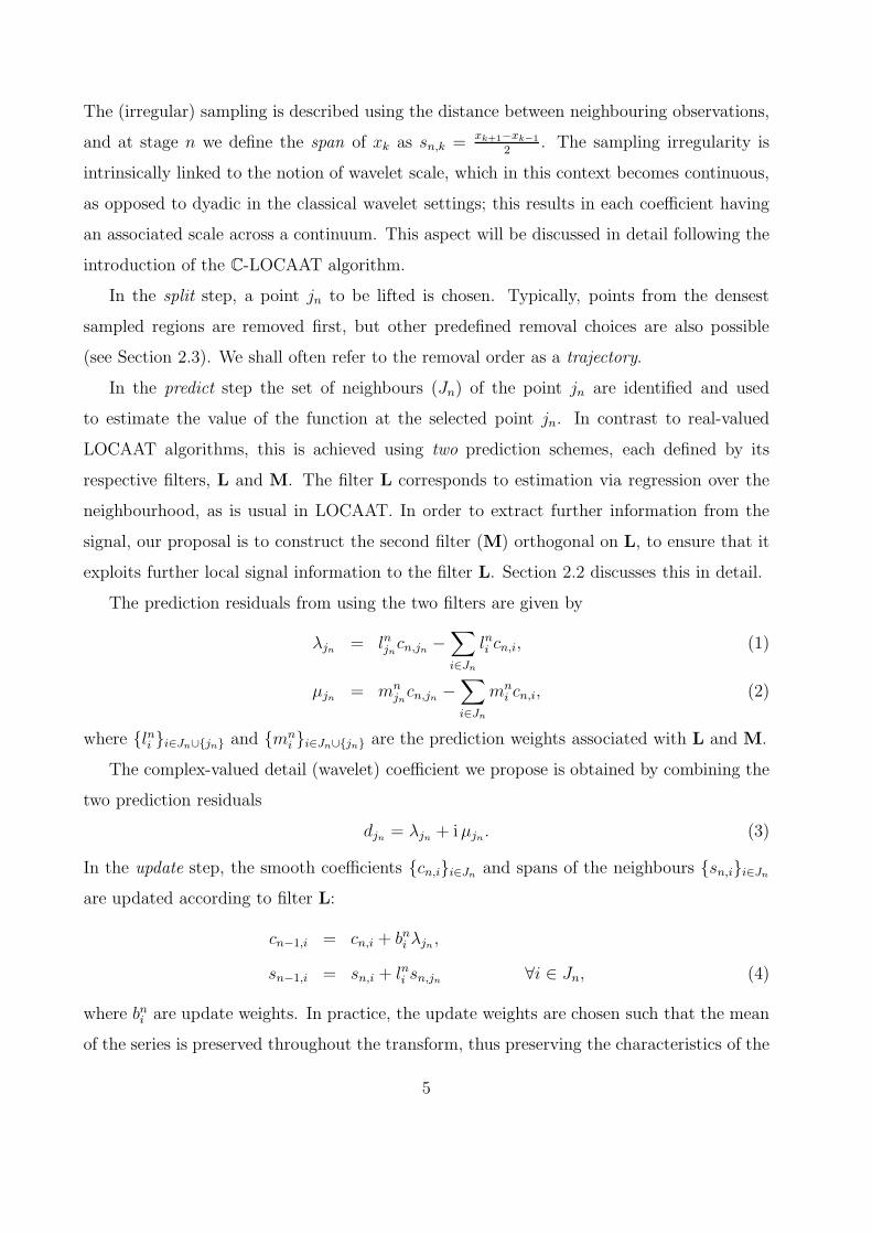
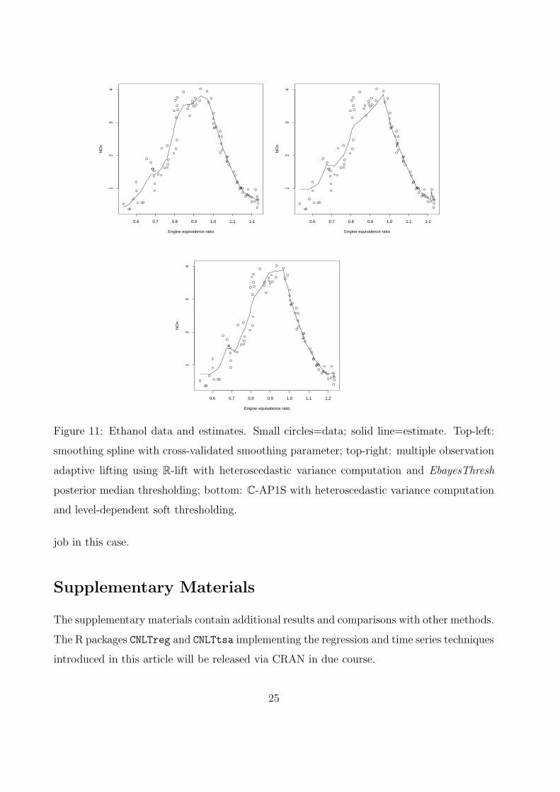
Note that our complex adaptive lifting estimate is very similar to the smoothing spline,

and both identify changes in slope around 0.7 and 0.9. However, the magnitude and duration

of these effects appear to be different between the two estimates. The real-valued adaptive

lifting estimate has an overall similar appearance albeit being less smooth and featuring

more abrupt changes that are unlikely to be true features of the process. In this example,

the true shape of the ethanol curve is of course unknown, however we believe that it is more

likely to be smooth. Hence it is pleasing to see that even visually our estimator does a good

24

0.6 0.7 0.8 0.9 1.0 1.1 1.2

12

34

Engine equivalence ratio

NO

x

0.6 0.7 0.8 0.9 1.0 1.1 1.2

12

34

Engine equivalence ratio

NO

x

0.6 0.7 0.8 0.9 1.0 1.1 1.2

12

34

Engine equivalence ratio

NO

x

Figure 11: Ethanol data and estimates. Small circles=data; solid line=estimate. Top-left:

smoothing spline with cross-validated smoothing parameter; top-right: multiple observation

adaptive lifting using R-lift with heteroscedastic variance computation and EbayesThresh

posterior median thresholding; bottom: C-AP1S with heteroscedastic variance computation

and level-dependent soft thresholding.

job in this case.

Supplementary Materials

The supplementary materials contain additional results and comparisons with other methods.

The R packages CNLTreg and CNLTtsa implementing the regression and time series techniques

introduced in this article will be released via CRAN in due course.

25

Acknowledgements

The authors would like to thank the two anonymous referees for helpful suggestions which led

to a much improved manuscript. Piotr Fryzlewicz’s work was supported by the Engineering

and Physical Sciences Research Council grant no. EP/L014246/1.

References

Abbas, A. and T. D. Tran (2006). Multiplierless design of biorthogonal dual-tree complex

wavelet transform using lifting scheme. In IEEE International Conference on Image Pro-

cessing. 2006, pp. 1605–1608. IEEE.

Abramovich, F., T. Bailey, and T. Sapatinas (2000). Wavelet analysis and its statistical

applications. Journal of the Royal Statistical Society D 49 (1), 1–29.

Allen, J. (1977). Short-term spectral analysis, and modification by discrete fourier transform.

IEEE Transactions on Acoustics Speech and Signal Processing 25 (3), 235–238.

Barber, S. and G. P. Nason (2004). Real nonparametric regression using complex wavelets.

Journal of the Royal Statistical Society B 66 (4), 927–939.

Bos, R., S. de Waele, and P. M. T. Broersen (2002). Autoregressive spectral estimation

by application of the Burg algorithm to irregularly sampled data. IEEE Transactions on

Instrumental Measurement 51 (6), 1289–1294.

Brinkman, N. D. (1981). Ethanol fuel-a single-cylinder engine study of efficiency and exhaust

emissions. Technical report, SAE Technical Paper.

Broerson, P. M. T. (2008). Time series models for spectral analysis of irregular data far

beyond the mean data rate. Measurement Science and Technology 19, 1–13.

Cleveland, W., E. Grosse, and W. Shyu (1992). Local regression models. In Statistical Models

in S. Chambers, J.M. and Hastie, T.J. (eds).

Engle, R. F. (2000). The econometrics of ultra-high-frequency data. Econometrica 68 (1),

1–22.

26

Erdogan, E., S. Ma, A. Beygelzimer, and I. Rish (2004). Statistical models for unequally

spaced time series. In Proceedings of the 5th SIAM International Conference on Data

Mining. SIAM.

Fernandes, F. C. A., I. W. Selesnick, R. L. C. van Spaendonck, and C. S. Burrus (2003).

Complex wavelet transforms with allpass filters. Signal Processing 83 (8), 1689–1706.

Foster, G. (1996). Wavelets for period analysis of unevenly sampled time series. The Astro-

nomical Journal 112 (4), 1709–1729.

Frick, P., A. Grossman, and P. Tchamitchian (1998). Wavelet analysis for signals with gaps.

Journal of Mathematical Physics 39, 4091–4107.

Gencay, R., M. Dacorogna, U. A. Muller, O. Pictet, and R. Olsen (2001). An Introduction

to High-Frequency Finance. Academic press.

Hall, P. and P. Patil (1996). On the choice of smoothing parameter, threshold and truncation

in nonparametric regression by non-linear wavelet methods. Journal of the Royal Statistical

Society B , 361–377.

Jacobsen, E. and R. Lyons (2003). The sliding DFT. IEEE Signal Processing Magazine 20 (2),

74–80.

Jansen, M., G. Nason, and B. Silverman (2001). Scattered data smoothing by empirical

bayesian shrinkage of second generation wavelet coefficients. In M. Unser and A. Aldroubi

(Eds.), Wavelet Applications in Signal and Image Processing IX, Volume 4478, pp. 87–97.

SPIE.

Jansen, M., G. P. Nason, and B. W. Silverman (2009). Multiscale methods for data on graphs

and irregular multidimensional situations. Journal Of The Royal Statistical Society Series

B 71 (1), 97–125.

Jansen, M. H. and P. J. Oonincx (2005). Second Generation Wavelets and Applications.

Springer Science & Business Media.

27

Kingsbury, N. (1999). Image processing with complex wavelets. Philosophical Transac-

tions of the Royal Society of London A: Mathematical, Physical and Engineering Sci-

ences 357 (1760), 2543–2560.

Kingsbury, N. (2001). Complex wavelets for shift invariant analysis and filtering of signals.

Applied and Computational Harmonic Analysis 10 (3), 234–253.

Knight, M. I. and G. P. Nason (2009). A ‘nondecimated’ lifting transform. Statistics and

Computing 19, 1–16.

Knight, M. I. and M. A. Nunes (2012). nlt: a nondecimated lifting scheme algorithm. R

package version 2.1-3.

Knight, M. I., M. A. Nunes, and G. P. Nason (2012). Spectral estimation for locally stationary

time series with missing observations. Statistics and Computing 22 (4), 877–895.

Kovac, A. and B. W. Silverman (2000). Extending the scope of wavelet regression meth-

ods by coefficient-dependent thresholding. Journal of the American Statistical Associa-

tion 95 (449), 172–183.

Lina, J.-M. and M. Mayrand (1995). Complex Daubechies wavelets. Applied and Computa-

tional Harmonic Analysis 2 (3), 219–229.

Loader, C. (1999). Local Regression and Likelihood. Springer: New York.

Lomb, N. (1976). Least-squares frequency analysis of unequally spaced data. Astrophysics

and Space Science 39 (2), 447–462.

Lutkepohl, H. (2005). New introduction to multiple time series analysis. Springer Science &

Business Media.

Magarey, J. and N. Kingsbury (1998). Motion estimation using a complex-valued wavelet

transform. IEEE Transactions on Signal Processing 46 (4), 1069–1084.

Nason, G. and B. Silverman (1995). The stationary wavelet transform and some applications.

In A. Antoniadis and G. Oppeheim (Eds.), Wavelets and Statistics, Volume 103 of Lecture

Notes in Statistics, pp. 281–300. New York: Springer-Verlag.

28

Nason, G. P. (2008). Wavelet Methods in Statistics with R. Springer.

Nason, G. P., R. von Sachs, and G. Kroisandt (2000). Wavelet processes and adaptive

estimation of the evolutionary wavelet spectrum. Journal of the Royal Statistical Society

B 62 (2), 271–292.

Nunes, M. A. and M. I. Knight (2012). adlift: an adaptive lifting scheme algorithm.

Nunes, M. A., M. I. Knight, and G. P. Nason (2006). Adaptive lifting for nonparametric

regression. Statistics and Computing 16 (2), 143–159.

Ombao, H., J. Raz, R. von Sachs, and W. Guo (2002). The SLEX model of a non-stationary

random process. Annals of the Institute of Statistical Mathematics 54 (1), 171–200.

Park, T., I. A. Eckley, and H. C. Ombao (2014). Estimating time-evolving partial coherence

between signals via multivariate locally stationary wavelet processes. IEEE Transactions

on Signal Processing 62, 5240–5250.

Percival, D. B. and A. T. Walden (2006). Wavelet Methods for Time Series Analysis, Vol-

ume 4. Cambridge University Press.

Portilla, J. and E. P. Simoncelli (2000). A parametric texture model based on joint statistics

of complex wavelet coefficients. International Journal of Computer Vision 40 (1), 49–70.

Priestley, M. B. (1983). Spectral Analysis and Time Series. Volumes I and II in 1 book.

Academic Press.

R Core Team (2013). R: A Language and Environment for Statistical Computing. Vienna,

Austria: R Foundation for Statistical Computing.

Rehfeld, K., N. Marwan, J. Heitzig, and J. Kurths (2011). Comparison of correlation analysis

techniques for irregularly sampled time series. Nonlinear Processes in Geophysics 18 (3),

389–404.

Reinsel, G. C. (2003). Elements of multivariate time series analysis. Springer Science &

Business Media.

29

Sanderson, J. (2010). Wavelet methods for time series with bivariate observations and irreg-

ular sampling grids. Ph. D. thesis, University of Bristol, UK. https://www.shef.ac.uk/

scharr/sections/heds/staff/hamilton_j.

Sanderson, J., P. Fryzlewicz, and M. W. Jones (2010). Estimating linear dependence between

nonstationary time series using the locally stationary wavelet model. Biometrika 97 (2),

435–446.

Scargle, J. (1982). Studies in astronomical time series analysis. II- Statistical aspects of

spectral analysis of unevenly spaced data. The Astrophysical Journal 263, 835–853.

Schroder, P. and W. Sweldens (1996). Building your own wavelets at home. ACM SIG-

GRAPH course notes .

Selesnick, I., R. Baraniuk, and N. Kingsbury (2005). The dual-tree complex wavelet trans-

form. IEEE Signal Processing Magazine 22 (6), 123–151.

Shui, P.-L., Z. Bao, and Y. Y. Tang (2003). Three-band biorthogonal interpolating complex

wavelets with stopband suppression via lifting scheme. IEEE Transactions on Signal

Processing 51 (5), 1293–1305.

Shumway, R. H. and D. S. Stoffer (2013). Time Series Analysis and its Applications. Springer

Science & Business Media.

Sweldens, W. (1996). The lifting scheme: A custom-design construction of biorthogonal

wavelets. Applied and Computational Harmonic Analysis 3 (2), 186–200.

Vanıcek, P. (1971). Further development and properties of the spectral analysis by least-

squares. Astrophysics and Space Science 12 (1), 10–33.

Witt, A. and A. Y. Schumann (2005). Holocene climate variability on millennial scales

recorded in greenland ice cores. Nonlinear Processes in Geophysics 12 (3), 345–352.

Wolff, E. W. (2005). Understanding the past-climate history from Antarctica. Antarctic

Science 17 (04), 487–495.

30