UNIT – IV chapter 1

RELATIONAL DATABASE DESIGN VIA ER MODELLING

Relational Database Design Using ER-to-Relational Mapping

Algorithm to convert the basic ER model constructs into relations

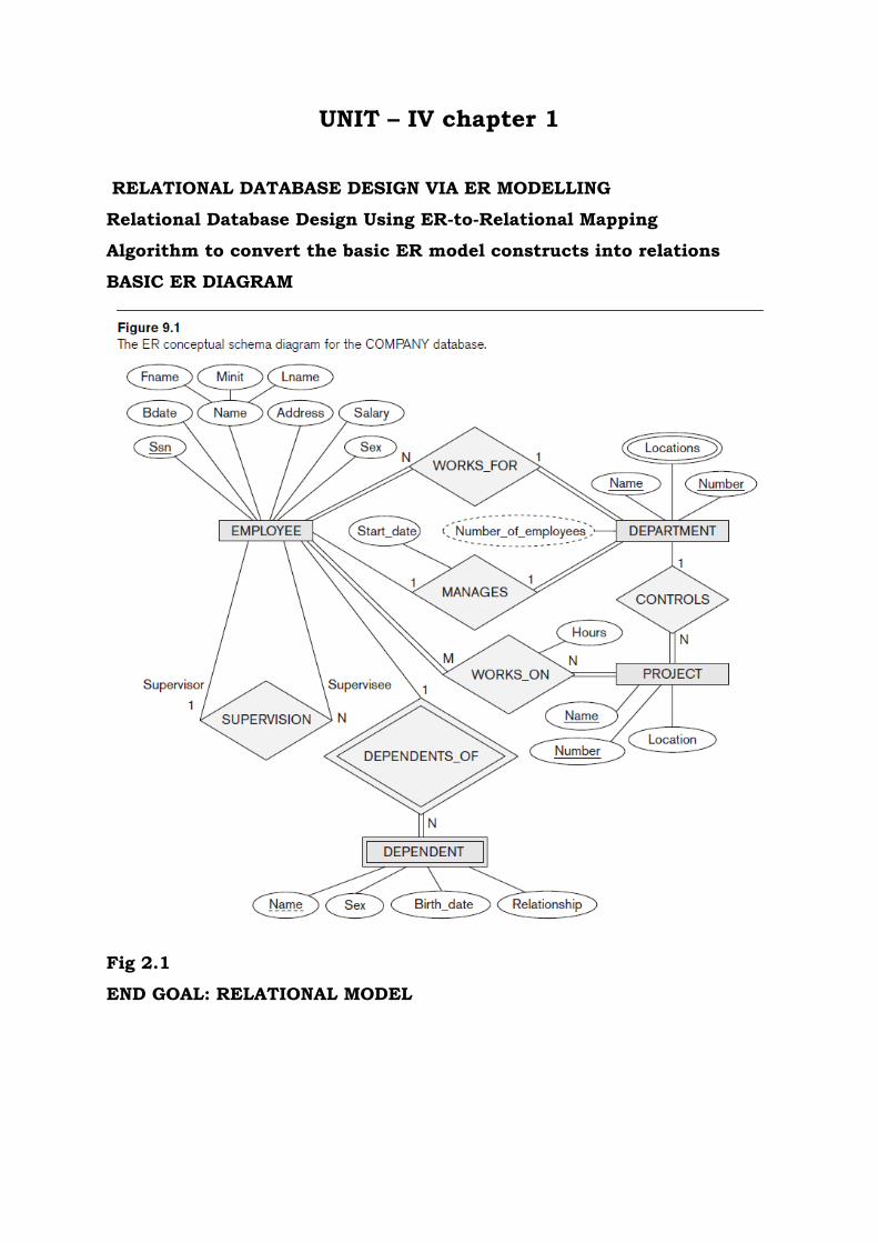
BASIC ER DIAGRAM

Fig 2.1

END GOAL: RELATIONAL MODEL

Fig 2.2

Step 1: Mapping of Regular Entity Types:

For each regular (strong) entity type E in the ER schema, create a

relation R that includes all the simple attributes of E.

Include only the simple component attributes of a composite attribute.

Choose one of the key attributes of E as primary key for R.

If the chosen key of E is composite, the set of simple attributes that

form it will together form the primary key of R.

In our example, we create the relations EMPLOYEE, DEPARTMENT,

and PROJECT in Figure 2.3 to correspond to the regular entity types

EMPLOYEE, DEPARTMENT, and PROJ ECT from Figure 2.1

Fig 2.3

Step 2: Mapping of Weak Entity Types:

For each weak entity type W in the ER schema with owner entity type

E, create a relation R and include all simple attributes of W as

attributes of R. In addition, include as foreign key attributes of R the

primary key Attribute(s) of the relation(s) that correspond to the owner

entity type(s): this takes care of the identifying relationship type of W

In our example, we create the relation DEPENDENT in this step to

correspond to the weakbentity type DEPENDENT.

We include the primary key SSN of the EMPLOYEE relation-which

corresponds to the owner entity type-as a foreign key attribute of

DEPENDENT

STEP 3: MAP BINARY 1:1 RELATIONSHIP TYPES:

For each binary 1:1 relationship type R, identify relation schemas that

correspond to entity types participating in R

Apply one of three possible approaches:

Foreign key approach

Add primary key of one participating relation as foreign key attribute

of the other, which will also represent R

If only one side is total, choose it to represent R

Declare foreign key attribute as unique

Merged relationship approach

An alternative mapping of a 1:1 relationship type is possible by

merging the two entity types and the relationship into a single relation.

This may be appropriate when both participations are total.

Cross-reference or relationship relation approach

Create new relation schema for R with two foreign key attributes being

copies of both primary keys

Declare one of the attributes as primary key and the other one as

unique

Add single-valued attributes of relationship type as attributes of R

Step 4: Mapping of Binary 1 :N Relationship Types:

For each regular binary l:N relationship type R, identify the relation S

that represents the participating entity type at the N-side of the

relationship type.

Include as foreign key in S the primary key of the relation T that

represents the other entity type participating in R; this is done

because each entity instance on the N-side is related to at most one

entity instance on the I-side Of the relationship type.

Include any simple attributes of the I:N relationship type as attributes

of S.

In our example, we now map the I:N relationship types WORKS_FOR,

CONTROLS, and SUPERVISION from Figure 2.1. For WORKS_FOR we

include the primary key DNUMBER of the DEPARTMENT relation as

foreign key in the EMPLOYEE relation and call it DNO.

For SUPERVISION we include the primary key of the EMPLOYEE

relation as foreign key in the EMPLOYEE relation itself because the

relationship is recursive-and call it SUPERSSN.

The CONTROLS relationship is mapped to the foreign key attribute

DNUM of PROJECT, which references the primary key DNUMBER of

the DEPARTMENT relation.

An alternative approach we can use here is again the relationship

relation option. We create a separate relation R whose attributes are

the keys of Sand T, and whose primary key is the same as the key of S

Step 5: Mapping of Binary M: N Relationship Types:

For each binary M:N relationship type R, create a new relation S to

represent R.

Include as foreign key attributes in S the primary keys of the relations

that represent the participating entity types; their combination will

form the primary key of S.

Also include any simple attributes of the M:N relationship type as

attributes of S.

Notice that we cannot represent an M:N relationship type by a single

foreign key attribute in one of the participating relations because of

the M:N cardinality ratio; we must create a separate relationship

relation S.

In our example, we map the M:N relationship type WORKS_ON from

Figure 2.1 by creating the relation WORKS_ON in Figure 2.3. We

include the primary keys of the PROJECT and EMPLOYEE relations

as foreign keys in WORKS_ON and rename them PNO and ESSN,

respectively.

We also include an attribute HOURS in WORKS_ON to represent the

HOURS attribute of the relationship type.

The primary key of the WORKS_ON relation is the combination of the

foreign key attributes {ESSN, PNO}.

1. INTRODUCTION TO RELATIONAL MODEL

The relational model is very simple and elegant: a relational database

is a collection of one or more relations, where each relation is a table

with rows and columns. This simple tabular representation enables

even novice users to understand the contents of a database, and it

permits the use of simple, high-level languages to query the data.

The major advantages of the relational model over the older data

models are its simple data representation and the ease with which

even complex queries can be expressed.

The relational model uses Data Definition Language (DDL) and Data

Manipulation Language (DML), the standard languages for creating,

accessing, manipulation and querying (i.e. retrieving) data in a

relational DBMS.

An important component of a relational model is that it specifies some

conditions that must be satisfied while accepting the values from the

user which prevents the entry of incorrect information. Such

conditions are called as Integrity Constraints (ICs), which enable the

DBMS to reject operations that might corrupt the data.

1.1 Fundamental Concepts in Relational Data Model

The main construct for representing data in the relational model is a

relation. A relation consists of a relation schema and a relation

instance.

The relation instance is a table, and the relation schema describes the

column heads for the table.

The schema specifies the relation's name, the name of each field (or

column, or attribute), and the domain of each field. A domain is

referred to in a relation schema by the domain name and has a set of

associated values.

An instance of a relation is a set of tuples, also called records, in

which each tuple has the same number of fields as the relation

schema. A relation instance can be thought of as a table in which

each tuple is a row, and all rows have the same number of fields. (The

term relation instance is often abbreviated to just relation, when there

is no confusion with other aspects of a relation such as its schema.)

Table 1.1: An Instance S1 of the Students Relation

The instance S1 contains six tuples and has, as we expect from the

schema, five fields. Note that no two rows are identical. This is a

requirement of the relational model-each relation is defined to be a set

of unique tuples or rows.

Domain:

A domain D is the original sets of atomic values used to model data.

By a atomic, we mean that each value in the domain is indivisible as

far as the relational model is concerned. A domain is a pool of the

values from where one or more attributes ( or columns) can draw their

actual values.

For Examples: The domain of name is the set of character strings that

represents names of person.

Tuple:

According to the model, every relation or table is made up of many

tuples.

They are also called the records. They are the rows that a table is

made up of.

Relation

A relation is a subset of the Cartesian product of a list of domains

characterized by a name. Given ‘n’ domains denoted by D1, D2, ..., Dn,

R is a relation defined on the these domains if R ≤ D1 * D2 * ... *Dn.

Relation can be viewed as a “table”.

In that table, each row represents a tuple of data values and each

column represents an attribute.

Attribute

A column of a relation designated by name. The name associated should be

meaningful. Each attributes associates with a domain. A relation schema

denoted by R is a list of attributes (A1, A2,...., An).

The Degree of the Relation

The degree of the relation is the number of attributes of its relation

schema. The degree of the relation of the Table 1.1 is 5.

The Cardinality of the Relation

The cardinality of the relation is the number of tuples in the relation.

The cardinality of the relation of the Table 1.1 is 6.

Characteristic of Relations

A tuple is a set of values. A relation is a set of tuples. Since a relation

is a set, there is no ordering on rows.

The order of attributes and their values within a relation is not

important as long as the correspondence between attributes and

values is maintained.

Each value in a tuple is atomic. That means each value cannot be

divided into smaller components. Hence, the composite and multi-

valued attributes are not allowed in a relation.

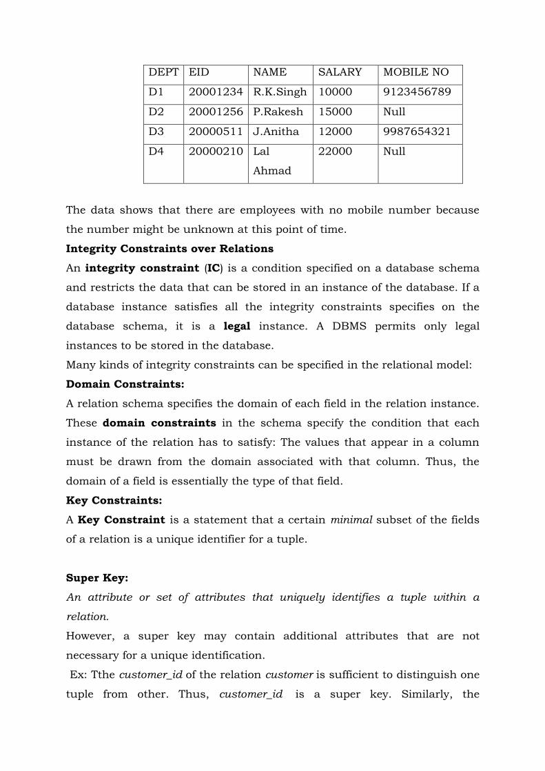
Table: The Relation Employee

DEPT EID NAME SALARY MOBILE NO

D1 20001234 R.K.Singh 10000 9123456789

D2 20001256 P.Rakesh 15000 Null

D3 20000511 J.Anitha 12000 9987654321

D4 20000210 Lal

Ahmad

22000 Null

The data shows that there are employees with no mobile number because

the number might be unknown at this point of time.

Integrity Constraints over Relations

An integrity constraint (IC) is a condition specified on a database schema

and restricts the data that can be stored in an instance of the database. If a

database instance satisfies all the integrity constraints specifies on the

database schema, it is a legal instance. A DBMS permits only legal

instances to be stored in the database.

Many kinds of integrity constraints can be specified in the relational model:

Domain Constraints:

A relation schema specifies the domain of each field in the relation instance.

These domain constraints in the schema specify the condition that each

instance of the relation has to satisfy: The values that appear in a column

must be drawn from the domain associated with that column. Thus, the

domain of a field is essentially the type of that field.

Key Constraints:

A Key Constraint is a statement that a certain minimal subset of the fields

of a relation is a unique identifier for a tuple.

Super Key:

An attribute or set of attributes that uniquely identifies a tuple within a

relation.

However, a super key may contain additional attributes that are not

necessary for a unique identification.

Ex: Tthe customer_id of the relation customer is sufficient to distinguish one

tuple from other. Thus, customer_id is a super key. Similarly, the

combination of customer_id and customer_name is a super key for the

relation customer. Here the customer_name is not a super key, because

several people may have the same name.

We are often interested in super keys for which no proper subset is a super

key. Such minimal super keys are called candidate keys.

Candidate Key:

A super key such that no proper subset is a super key within the relation.

There are two parts of the candidate key definition:

i. Two distinct tuples in a legal instance cannot have identical values in

all the fields of a key.

ii. No subset of the set of fields in a candidate key is a unique identifier

for a tuple.

A relation may have several candidate keys.

Ex: The combination of customer_name and customer_street is sufficient to

distinguish the members of the customer relation. Then both, {customer_id}

and {customer_name, customer_street} are candidate keys. Although

customer_id and customer_name together can distinguish customer tuples,

their combination does not form a candidate key, since the customer_id

alone is a candidate key.

Primary Key:

The candidate key that is selected to identify tuples uniquely within the

relation. Out of all the available candidate keys, a database designer can

identify a primary key. The candidate keys that are not selected as the

primary key are called as alternate keys.

Features of the primary key:

i. Primary key will not allow duplicate values.

ii. Primary key will not allow null values.

iii. Only one primary key is allowed per table.

Ex: For the student relation, we can choose student_id as the primary key.

Foreign Key:

Foreign keys represent the relationships between tables. A foreign key is a

column (or a group of columns) whose values are derived from the primary

key of some other table.

The table in which foreign key is defined is called a Foreign table or Details

table. The table that defines the primary key and is referenced by the foreign

key is called the Primary table or Master table.

Features of foreign key:

Records cannot be inserted into a detail table if corresponding records in

the master table do not exist.

Records of the master table cannot be deleted or updated if

corresponding records in the detail table actually exist.

General Constraints:

Domain, primary key, and foreign key constraints are considered to be a

fundamental part of the relational data model. Sometimes, however, it is

necessary to specify more general constraints.

For example, we may require that student ages be within a certain range of

values. Giving such an IC, the DBMS rejects inserts and updates that violate

the constraint.

Current database systems support such general constraints in the form of

table constraints and assertions. Table constraints are associated with a

single table and checked whenever that table is modified. In contrast,

assertions involve several tables and are checked whenever any of these

tables is

INTRODUCTION TO SCHEMA REFINEMENT

Conceptual database design gives us a set of relation schemas and integrity

constraints (ICs) that can be regarded as a good starting point for the final

database design. This initial design must be refined by taking the ICs into

account and also by considering performance criteria and typical workloads.

A major aim of relational database design is to minimize data redundancy.

The problems associated with data redundancy are illustrated as follows:

Problems caused by redundancy

Storing the same information in more than one place within a database is

called redundancy and can lead to several problems:

Redundant Storage: Some information is stored repeatedly.

Update Anomalies: If one copy of such repeated data is updated, an

inconsistency is created unless all copies are similarly updated.

Insertion Anomalies: It may not be possible to store certain

information unless some other, unrelated, information is stored as

well.

Deletion Anomalies: It may not be possible to delete certain

information without losing some other, unrelated, information as well.

Ex: Consider a relation, Hourly_Emps(ssn, name, lot, rating, hourly_wages,

hours_worked)

The key for Hourly_Emps is ssn. In addition, suppose that the hourly_wages

attribute is determined by the rating attribute. That is, for a given rating

value, there is only one permissible hourly_wages value. This IC is an

example of a functional dependency. It leads to possible redundancy in the

relation Hourly_Emps, as shown below:

ssn name

lot

rating

hourly_wages hours_worked

567 Adithya 48 8 10 40

576 Devesh 22 8 10 30

574 Ayush

Soni

35 5 7 30

597 Rajasekhar 35 5 7 32

5c1 Sunil 35 8 10 40

If the same value appears in the rating column of two tuples, the IC tells us

that the same value must appear in the hourly_wages column as well. This

redundancy has the following problems:

Redundant Storage: The rating value 8 corresponds to the

hourly_wage 10, and this association is repeated three times.

Update Anomalies: The hourly_wage in the first tuple could be

updated without making a similar change in the second tuple.

Insertion Anomalies: We cannot insert a tuple for an employee unless

we know the hourly_wage for the employee’s rating value.

Deletion Anomalies: If we delete all tuples with a given rating value

(e.g., we delete the tuples for Ayush Soni and Rajasekhar) we lose the

association between that rating value and its hourly_wage value.

Null Values

Null values cannot provide a complete solution, but they can provide some

help.

Consider the example Hourly_Emps relation. Here null values cannot help to

eliminate redundant storage, update or deletion anomalies. It appears that

they can address insertion anomalies. For instance, we can insert an

employee tuple with null values in the hourly wage field. However, null

values cannot address all insertion anomalies. Thus, null values do not

provide a general solution to the problems of redundancy, even though they

can help in some cases.

Decompositions

A decomposition of relation schema R consists of replacing the relation

schema by two or more relation schemas that each contain a subset of the

attributes of R and together include all attributes in R.

Ex: We can decompose Hourly_Emps into two relations:

Hourly_Emps2(ssn, name, lot, rating, hours_worked)

Wages(rating, hourly_wages)

Problems Related to Decomposition

Two important questions must be asked during decomposition process:

1. Do we need to decompose a relation?

2. What problems does a given decomposition cause?

To answer a first question, several normal forms have been proposed for

relations. If a relation schema is in one of these normal forms, we know that

certain kinds of problems cannot arise.

With respect second question, two properties of decomposition are to be

considered:

The lossless-join property enables us to recover any instance of the relation

of the decomposed relation from corresponding instances of the smaller

relations.

The dependency-preservation property enables us to enforce any constraint

on the original relation by simply enforcing some constraints on each of the

smaller relations. That is, we need not perform joins of the smaller relations

to check whether a constraint on the original relation is violated.

Functional Dependencies

A functional dependency (FD) is a kind of IC that generalizes the concept

of a key.

Let R be a relation schema and let X and Y be nonempty sets of attributes in

R. We say that an instance r of R satisfies the FD X→Y1 if the following holds

for every pair of tuples t1 and t2 in r:

If t1.X = t2.X, then t1.Y = t2.Y.

An FD X→Y says that if two tuples agree on the values in attributes X, they

must also agree on the values in attributes Y.

Ex: The FD AB→C is satisfied by the following instance:

A B C D

1 X→ Y is read as X functionally determines Y, or simply as X determines Y.

a1 b1 c1 d1

a1 b1 c1 d2

a1 b2 c2 d1

a2 b1 c3 d1

Here, if we add a tuple <a1, b1, c2, d1> to the instance shown in figure, the

resulting instance would violate the FD.

Reasoning about FDs

Given a set of FDs over a relation schema R, typically several additional FDs

hold over R whenever all of the given FDs hold.

Ex: Consider Workers(ssn, name, lot, did, since)

With given FDs ssn → did and did→ lot. Then, in any legal instance of

Workers, if two tuples have the same ssn value, they must have the same

did value, and because they have the same did value, they must also have

the same lot value. Therefore, the FD ssn→ lot also holds on Workers.

Closure of a Set of FDs

The set of all FDs implied by a given set F of FDs is called the closure of F,

denoted as F+. The closure F+ can be calculated by using the following

Armstrong’s Axioms rules. Let X, Y, and Z be the sets of attributes over a

relation schema R:

Reflexivity: If X is a super set of Y, then X→Y.

Augmentation: If X→Y, then XZ→YZ for any Z.

Transitivity: If X→Y and Y→Z, then X→Z.

Union: If X→Y and X→Z, then X→YZ.

Decomposition: If X→YZ, then X→Y and X→Z.

Ex1:

Consider a relation schema ABC with FDs A→B and B→C.

From transitivity, we get A→C.

From augmentation, we get AC→BC, AB→AC, AB→CB.

Ex2:

Contracts(contractid, supplierid, projectid, deptid, partid, qty, value)

We denote the schema for Contracts as CSJDPQV.

The following are the given FDs:

i) C→ CSJDPQV.

ii) JP→C.

iii) SD→P.

Several additional FDs hold in the closure of the set of given FDs:

From JP→C and C→CSJDPQV, and transitivity, we infer JP→CSJDPQV.

From SD→P and augmentation, we infer SDJ→ JP.

From SDJ→JP, JP→CSJDPQV, and transitivity, we infer SDJ→CSJDPQV.

Note:

In a trivial FD, the right side contains only attributes that also

appear on the left side. Using reflexivity, we can generate all trivial

dependencies, which are of the form:

X→Y, where Y is a subset of X, X is a subset of ABC, and Y is a subset

of ABC.

From augmentation, we get the nontrivial dependencies.

Attribute Closure

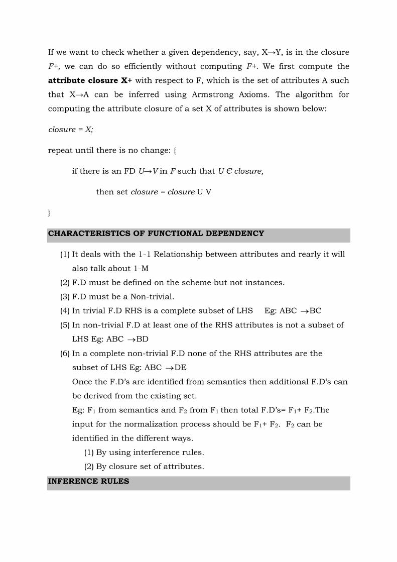
If we want to check whether a given dependency, say, X→Y, is in the closure

F+, we can do so efficiently without computing F+. We first compute the

attribute closure X+ with respect to F, which is the set of attributes A such

that X→A can be inferred using Armstrong Axioms. The algorithm for

computing the attribute closure of a set X of attributes is shown below:

closure = X;

repeat until there is no change: {

if there is an FD U→V in F such that U Є closure,

then set closure = closure U V

}

CHARACTERISTICS OF FUNCTIONAL DEPENDENCY

(1) It deals with the 1-1 Relationship between attributes and rearly it will

also talk about 1-M

(2) F.D must be defined on the scheme but not instances.

(3) F.D must be a Non-trivial.

(4) In trivial F.D RHS is a complete subset of LHS Eg: ABC BC

(5) In non-trivial F.D at least one of the RHS attributes is not a subset of

LHS Eg: ABC BD

(6) In a complete non-trivial F.D none of the RHS attributes are the

subset of LHS Eg: ABC DE

Once the F.D’s are identified from semantics then additional F.D’s can

be derived from the existing set.

Eg: F1 from semantics and F2 from F1 then total F.D’s= F1+ F2.The

input for the normalization process should be F1+ F2. F2 can be

identified in the different ways.

(1) By using interference rules.

(2) By closure set of attributes.

INFERENCE RULES

(1) Reflexive: If ‘B’ is a subset of ‘A’ then always ‘A’ can determine ‘B’

BA

(2) Augmentation: If BA then BCAC

(3) Transitive: If BA and B C then CA

(4) Union: It is applied for the LHS attributes i.e., If BA , CA then

BCA

(5) Decomposition: If BCA then we can write it as BA and CA

(6) Composition: If BA and DC then, BDAC

(7) Self determination: AA , BB

1Q Find the additional F.D’s derived from F1 where a set of F.D’s from

semantics.

HFHG)8(

GF)7(

FE)6(

EHDHD)5(

ED)4(

DC)3(

CACB)2(

BA)1(

F2=

HF

EHD

CA

By transitive rule, CA from (1) & (2)

By union rule, EHD from (4) & (5)

By transitive rule, HF from (7) & (8)

CLOSURE SET OF ATTRIBUTES

Algorithm used to identify the closure set of attributes:

(1) Let ‘X’ be a set of attributes that will become the closure.

(2) Repeatedly search for a F.D where the LHS of F.D is a part of ‘X’ then

add RHS of the F.D to ‘X’ is already not available.

(3) Repeat step (2) as many times as necessary until no more attributes

can be added to ‘X’.

(4) The set ‘X’ after no more attributes can be added to ‘X’ will become a

closure set.

Applications of closure set of attributes:

(1) To identify the additional F.D’s.

(2) To identify the keys.

(3) To identify the equivalences of the F.D’s

(4) To identify irreducible set of F.D’s or canonical forms of F.D’s or

standard form of F.D’s.

2Q Consider a relation ABCDEFG and FDs are

ACFind

GAEG

DEBC

BA

Ans: X= AC

= ACB

= ABCDE

AC = ABCDE

3Q For the relation R(ABCDE) and FDs are

CD&AB,BFind

AE

DB

ECD

BCA

Ans: X =B

=BD

B+ =BD

Find AB+

X = AB

= ABC

= ABCD

=ABCDE

AB = ABCDE

Find CD+

X = CD

= CDE

= ACDE

=ABCDE

CD = ABCDE

4Q For a relation R(ABCDEF) and FDs are

ABFind

BCF

ED

ADBC

CAB

Ans: Find AB+

X= AB

= ABC

= ABCD

=ABCDE

AB = ABCDE

(1) Identifying the additional F.D’s

To check any F.D’s like BA can be determined from F1 or not.

Complete A+ from F1 is A+ includes B also then, BA can be derived

as a F.D in F2.

Q5 Check AD can be derived from F1

F1:

BCF

ED

ADBC

CAB

i. DA

X =D

=DE

D+=DE

D A i.e. Cannot be determine A

ii. ABD

X=AB

=ABC

=ABCD

AB+=ABCD

iii.ABF

X=AB

=ABC

=ABCD

=ABCDE

AB+=ABCDE

AB↛ F cannot be determine F

Q6 Find BCDH can be derived from F1

F1:

BCDH

BDAEH

AEHD

CE

ECD

BCA

Sol:

i. X=BCD

=BCDE

=BCDEH

=BCDEAH

BCD+=BCDEAH

BCDH

(ii) ABCH

X=ABC

ABC H

(2) Identification of key by using closure set as attributes

(i) A primary key

(ii) Composite primary ey

(iii)Candidate keys

(iv) Foreign keys

(v) Surrogate key

(vi) Super key

Max.no.of Foreign keys=1024.

A key attribute: An attribute that is capable of identifying all other

attributes in a given table.

(i) Primary key:

It is an unique value attribute in a table to enforce entity

integrity and ti identify rows in the table uniquely.

(ii) Composite Primary Key:

Sometimes single attribute is not sufficient to identify uniquely the

rows in the table so, we combine 2 or more attributes to identify the

rows uniquely.

(iii) Candidate keys:

Sometimes 2 or more independent attribute or attributes can be used

to identify the rows uniquely Eg :( vech no,veng no,purchase date)

Either vehicle no or vehicle engine no can be used as a key attribute

then they are called as candidate keys one of the candidate key can be

elected as primary key.

(iv) Surrogate key:

Sometimes even if you combine all the attributes in the table they may

not have unique values.

To identify the rows uniquely we will use a system generated key

called as surrogate key.

(v) Foreign key:

It is used to enforce referential integrity and an attribute in a table

can be called as a foreign key attribute that refer primary key in same

or different table.

Q1 If R(ABCDEH) and FDs are

BCDH

BDAEH

AEHD

CE

ECD

BCA

Find keys?

Super key=ABCDEH

Now find A+=ABC

E+=EC

D+=DAEH

=ABCDEH

D is key

If the closure of any of the LHS attributes are combinations of

the LHS attributes includes all the attributes in the table then

that will become a key in the table.

A table can have 2 or more keys.

Q2 Consider a relation with five attributes ABCDE and FDs are

AED

EBC

BA

List all keys for R.

Sol: Super key: ABCDE

A+=AB X

BC+=BCE X

ED+=ABDE X

AB+=AB X

AC+=ABCE X

BD+=BD X

ABC+=ABCE

BCD+=BCDEA

ACD+=ABCDE

CDE+=ADEBC

Q3 R(ABCDE) & FDs are

BDE

ECD

CAB

List all keys for R.

Sol: Super key=ABCDE

AB+=ABC

CD+=CDE

DE+=DEB

ABC+=ABC

ABD+=ABDCE

ABE+=ABEC

ACD+=ACDEB

ABD & ACD are keys

Q4 R(ABCDEGGHIJ) &FDs are

RJD

GHF

FB

DEA

CAB

List all keys for R

Note:

Sometimes all the attributes in the table may not appear in F.D’s

Eg: D I may be available instead of D IJ

AB+=ABCDEFGHIJ

The key for the relation R=ABJ the missing attributes from the F.D’s

must be attached to the closure.

Q5 R(ABCDEFGHIJ) & FDs are

JH

IA

GHAD

EFBD

CAB

List all keys for R

Sol:

Super key=ABDH

AB+=ABC X

BD+=BDEF X

AD+=ADGHIJ X

ABD+=ABDCEFGHIJ

ABH+=ABHCIJ X

ABD+=ABCDEFGHIJ

(3) To identify equivalence of F.D

Different database designers may define different F.D’s sets from the

same requirements.To evaluate whether they are equivalent if we are

able to derive all F.D’s in G from F and vice-versa.

Q1 Consider the following two sets of FDs

F=

HE

ADE

DAC

CA

G = AHE

CDA

Find the equivalence of two sets of FDs.

Step 1: Take set F and enclose all FD’s in G that can be derived from F.

CDA

A+ from F

X=A

=AC

=ACD

FfromderivedbecanCDA

AHE

E+ from F

X=E

=EAD

=EADH

FfromderivedbecanAHE

Step 2: Take set G and enclose all F.D’s in F that can be derived from G.

CA

A+ from G

X=A

=ACD

GfromderivedbecanCA

X=AC

=ACD

ADE

X=E

=EAH

=EAHCD

ADfromGEAHE &

F G so, G is preferable as it contains less FDs.

Q2 Consider two sets of FDs on the attributes ABCDE

F=

AB

EAD

CDB

G=

EAD

ABCB

CDEB

Find whether they are equivalent or not

Sol:

Step 1:

CDEB

B+ from F

X=B

=BCDA

=ABCDE

All FD’s are derivable from F.

Step 2:

CDB

B+ from G

X=B

=BCDE

=ABCDE

All FD’s are derivable from G.

F G

F is preferable

No of dependencies are less.

(4) To identify the irreducible form of FD’s /canonical Form

Once F1 is identified from the semantics and F2 is derived from F1 we

get total F.D’s i.e F but before making a move to the normalization

process with F,F must be evaluated for redundant attribute on the LHS

and RHS of F.D’s and it is a four step process.

Step 1: Have single attributes on the RHS for every FD.

Step 2: Evaluate all F.D’s in step 1 for their necessity. If they are not

necessary, remove them from the list.

Step 3: Evaluate the necessity of the RHS attributes in FD’s obtained from

step 2.If they are not necessary remove from FD.

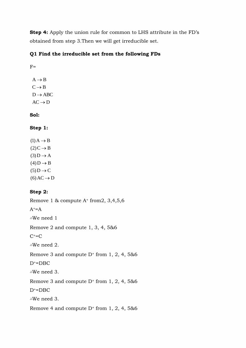
Step 4: Apply the union rule for common to LHS attribute in the FD’s

obtained from step 3.Then we will get irreducible set.

Q1 Find the irreducible set from the following FDs

F=

DAC

ABCD

BC

BA

Sol:

Step 1:

DAC)6(

CD)5(

BD)4(

AD)3(

BC)2(

BA)1(

Step 2:

Remove 1 & compute A+ from2, 3,4,5,6

A+=A

We need 1

Remove 2 and compute 1, 3, 4, 5&6

C+=C

We need 2.

Remove 3 and compute D+ from 1, 2, 4, 5&6

D+=DBC

We need 3.

Remove 3 and compute D+ from 1, 2, 4, 5&6

D+=DBC

We need 3.

Remove 4 and compute D+ from 1, 2, 4, 5&6

D+=ADCB

D B can be removed.

Remove 5 and compute D+ from 1, 2, 3,4&6

D+=ABD

We need 5.

Remove 6 and compute D+ from 1, 2,3, 4, 5

AC+=ACB

We need 6.

Step 3:

DAC

CD

AD

BC

BA

Remove A

DC

CD

AD

BC

BA

DAC

CD

AD

BC

BA

C+=CDAB C+=CB

C+ C+

Remove C

DA

CD

AD

BC

BA

DAC

CD

AD

BC

BA

A+=ADCB A+=AB

A+ A+

Step 4:

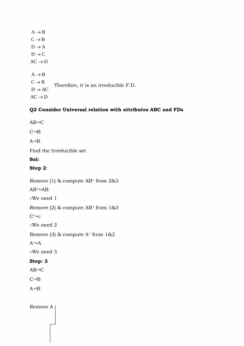
DAC

CD

AD

BC

BA

DAC

ACD

BC

BA

Therefore, it is an irreducible F.D.

Q2 Consider Universal relation with attributes ABC and FDs

AB C

C B

A B

Find the Irreducible set

Sol:

Step 2:

Remove (1) & compute AB+ from 2&3

AB+=AB

We need 1

Remove (2) & compute AB+ from 1&3

C+=c

We need 2

Remove (3) & compute A+ from 1&2

A+=A

We need 3

Step: 3

AB C

C B

A B

Remove A

AB C B C

C B C B

A B A B

B+=B B+=BC

B+ B+

Remove B

AB C A C

C B C B

A B A B

A+=ABC A+=ACB

A+=A+

B can be removed

Step 4:

A C

C B

A B

A BC & C B it is an irreducible set.

Q3 FDs are

F= ABD AC

C BE

AD BF

B E

Find the minimal set

Step 1:

ABD A

ABD C

C B

C E

AD B

AD F

B E

Remove (1) & compute ABD+ from (2-7)

ABD+ =ABDCEF

(1) can be removed

Remove (2) & compute ABD+ from (1,3-7)

ABD+ =ABDEF

We need (2)

Remove (3) & compute C+ from (1,2,4-7)

C+ =CE

We need (3)

Remove (4) & compute C+ C+ =BCE

(4) Can be removed

Remove (5) & compute AD+

AD+ =ADF

We need (5)

Remove (6) & compute AD+

AD+ =ADBCE

We need (6)

Remove (7) & compute B+

B+ =B

We need (7)

Step 3:

ABD C

C B

AD B

AD F

B E

Remove A

ABD C BD C

C B C B

AD B AD B

AD F AD F

B E B E

BD+=BDE BD+=BDCE

BD+ BD+

Remove B

ABD C AD C

C B C B

AD B AD B

AD F AD F

B E B E

AD+=ABFECD AD+=ADCFBE

AD+= AD+

B can be removed.

Types of functional Dependencies:

(1) Partial F.D

(2) Transitive F.D

(3) Full F.D.

1. Partial F.D: A dependency in which non-key attributes are partially

depending on key attributes.

R=ABCD

F=AB C

=B D

Key: AB but B is depending only D therefore B D is considered as

partial dependency

Under the following conditions a table cannot have partial F.D

(1) If primary key consists a single attribute

(2) If table consists only two attributes

(3) If all the attributes in the table are part of the primary key.

2. Transitive F.D: A dependency in which there is a relationship among

the non-key attributes.

Eg:R=ABCD

F: AB C

AB D

C D

Key=AB

C d Is a transitive dependency and it causes insertion, deletion &

updation problems in the table.

Under the following Circumstances, a table cannot have transitive F.D

(1) If table consists only two attributes

(2) If all the attributes in the table are part of the primary key.

3. Full F.D:A dependency X Y is considered as a full F.D if the removal

of any attribute from X makes X Y as invalid F.D

Eg: AB CD

B CDX

AB CD is a full F.D

NORMALIZATION

It is the process of reducing the redundancy based on primary keys

and F.D

OR

It is a tool to validate or evaluate the logical database design with the

help of rules which are called as Normal Forms. They are

1 NF

2 NF

3 NF

BCNF Problem intensity reduces and no. of tables needed will be

increased.

4 NF

5 NF

DKNF

Points to be Remember

1 NF is a mandatory NF and remaining are the optional

If you construct E-R diagrams in to the tables, then 4 NF and 5 NF

need not be applied on the table.

Practically applied normalization is upto 3NF and very rarely we will

go beyond that.

2 NF dealing with the partial dependencies and 3NF is dealing with

transitive dependencies.

First Normal Form (1NF):

The cells of the table must have single atomic value

Neither repeating groups nor arrays are allowed as values

All entries in any column (attribute)must be of the same kind

Each column must have a unique name, but the order of the columns

in the table is insignificant.

No two rows in a table may be identical and the order of rows is

insignificant

Second Normal Form (2 NF):

A table is said to be in 2NF if it is already in the 1NF and free from

Partial dependency.

Anomalies can occur when attributes are dependent on only part of a

multi-attribute key.

A relation is in second normal form when all non-key attributes are

dependent on the whole key.

Any relation having a key with a single attribute is in second normal

form

Q1 Consider universal relation R=ABCDEFGHIJ and the set of FDs are

F=AB C

A DE

B F

F GH

D IJ

What is the key for R? Decompose R into 2NF

Sol: key=AB

AB=CDEFGHIJ

Step 1: A B C D E F G H I J

Or

A+=ADEIJ

B+=BFGH

If there is a partial dependency, remove partially dependent attributes from

the original table and place it in a separate table along with the copy of its

determinant.

(a) Key =AB

(b) A+=ADEIJ

B+=BFGH

DEIJ-depending only on A

FGH-depending only on B

(c)

ABC=R

BFGH=R

ADEIJ=R

3

2

1

R=ABC

Required 2 NF

Q2 Consider the relation R=ABCDEF and set of FDs are

F=A FC

C D

B E

Find the key and normalize into 2NF

Sol:

(a) Key=AB

(b) A+=ACDF

B+=BE

(c)

AB=R

BE=R

ACDF=R

3

2

1

R=AB

Requried 2 NF

Q3 Consider the relation R=ABCDE. Find the key and normalize upto 2NF

F=B E

C D

A B

Sol:(A) KEY=AC

(B) A+=ABE

C+=CD

(C) R=A

AC=R

CD=R

ABE=R

3

2

1

Required 2 NF

Q4 Consider R= ABCDEFGHIJ and FDs are

F=AB C

BD EF

AD GH

A I

H J

Find the key and normalize upto 2NF

Sol: (A) Key=ABD

(B) AB+=ABCI

BD+=BDEF

AD+=ADGHIJ

(C)R1=ABCI A+=AI R11=AI

B+=B R111=ABC

R2=BDEF B+=B R2=BDEF

D+=D

R3=ADGHIJ A+=AI R31=AI

D+=D R311=ADGHJ

R4=ABD

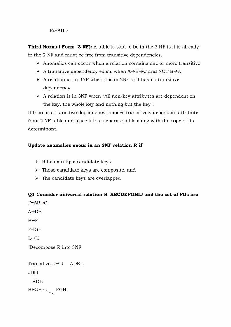
Third Normal Form (3 NF): A table is said to be in the 3 NF is it is already

in the 2 NF and must be free from transitive dependencies.

Anomalies can occur when a relation contains one or more transitive

A transitive dependency exists when ABC and NOT BA

A relation is in 3NF when it is in 2NF and has no transitive

dependency

A relation is in 3NF when “All non-key attributes are dependent on

the key, the whole key and nothing but the key”.

If there is a transitive dependency, remove transitively dependent attribute

from 2 NF table and place it in a separate table along with the copy of its

determinant.

Update anomalies occur in an 3NF relation R if

R has multiple candidate keys,

Those candidate keys are composite, and

The candidate keys are overlapped

Q1 Consider universal relation R=ABCDEFGHIJ and the set of FDs are

F=AB C

A DE

B F

F GH

D IJ

Decompose R into 3NF

Transitive D IJ ADEIJ

DIJ

ADE

BFGH FGH

BP

ABC ABC

NF3sinIti

ABCR

BFR

FGH=R

ADE=R

DIJ=R

5

4

3

2

1

Q2 Consider the relation R=ABCDEF and set of FDs are

F=A FC

C D

B E

Normalize R into 3NF

ACDF CD

ACF

BE BE

𝐴𝐵 →AB

NFin

AB

3

R

BE=R

ACF=R

CD=R

4

3

2

1

Q3 Consider the relation R=ABCDE. Find the key and normalize upto 3NF

F=B E

C D

A B

R1=ABE BE

AB

ABC

BF

5

4

3

2

1

R

R

FGH=R

ADE=R

DIJ=R

R2=CD CD

R3=AC AC

NF3sinIti

ACR

CD=R

AB=R

BE=R

4

3

2

1

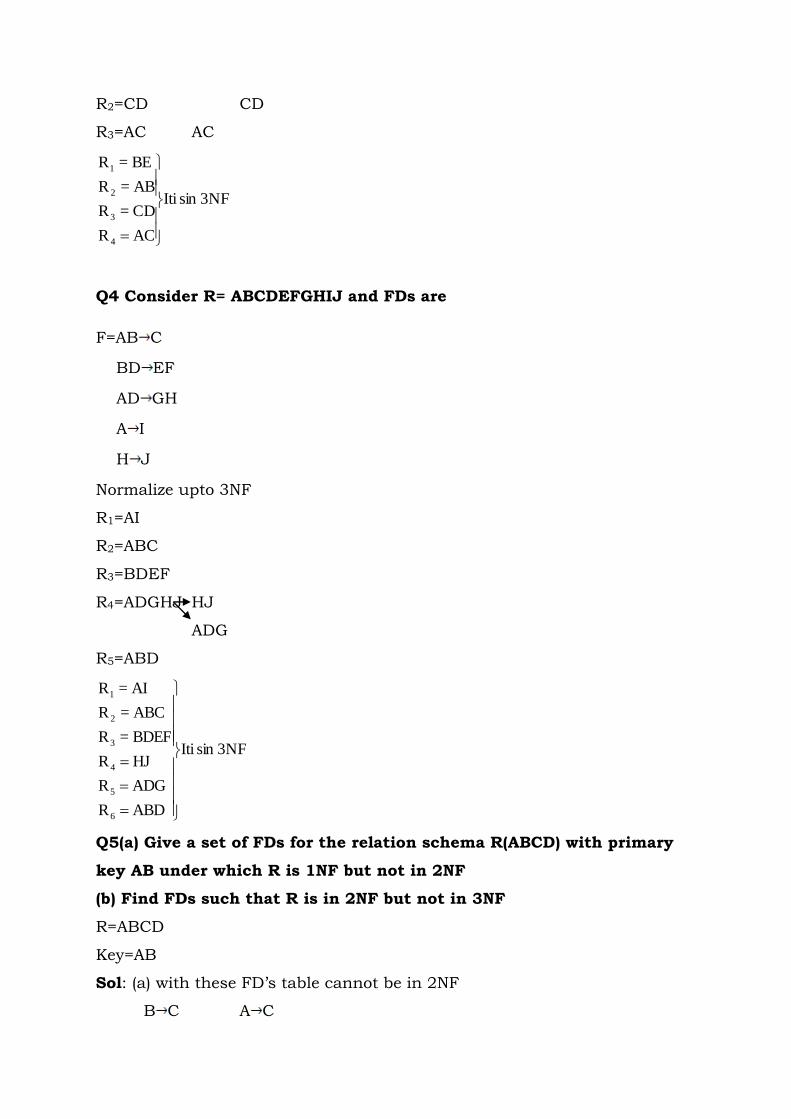
Q4 Consider R= ABCDEFGHIJ and FDs are

F=AB C

BD EF

AD GH

A I

H J

Normalize upto 3NF

R1=AI

R2=ABC

R3=BDEF

R4=ADGHJ HJ

ADG

R5=ABD

NF3sinIti

ABDR

ADGR

HJR

BDEF=R

ABC=R

AI=R

6

5

4

3

2

1

Q5(a) Give a set of FDs for the relation schema R(ABCD) with primary

key AB under which R is 1NF but not in 2NF

(b) Find FDs such that R is in 2NF but not in 3NF

R=ABCD

Key=AB

Sol: (a) with these FD’s table cannot be in 2NF

B C A C

B D A D

(b ) with these FD’s the table may be in 2NF but not in 3NF

C D D C

Note 1: In general if bxorAxandAorBif;x (key=AB) then it will

violate 2 NF

Note 2: In general, if I have x→ BorAwith; and x is not a proper

set of AB then it will violet 3NF but not 2 NF.

Note 3: If there is a F.D x y,It is allowed in 3NF(also in 2NF) if x is a

super key or y is a part of key.

Lossless join property and dependency preserving:

In a good database design, it is not only sufficient to check whether

tables are satisfying 2NF, 3NF & BCNF but also check whether

decomposed tables are satisfying the following two properties.

(1) Lossless join Property(mandatory)

(2) Dependency Preserving Property(optional)

Lossless join Property:

A decomposition of R into R1,R2,R3,…..Rn is said to a loss less

decomposition if the natural joint of all the projections of R must give the

original relation i.e R= )R()......R()R( Rn2R1R suppose, if

)R().......R()R(R Rn2R1R then decomposition is said to be lossy

decomposition.

Q:

R:

A B C

a1 b1 c1

a2 b2 c2

a3 b1 c3

R1

R2

`

∴ )R()R(R 2R1R

A B C

a1 b1 c1

a1 b1 c3

a2 b2 c2

a3 b1 c1

a3 b1 c3

5 rows

Lossy decomposition

The above method is a time consuming and error prone there fore,to check

the lossless joint property we use the following short cut method.

A B

a1 b1

a2 b2

a3 b1

B C

b1 c1

b2 c2

b1 c3

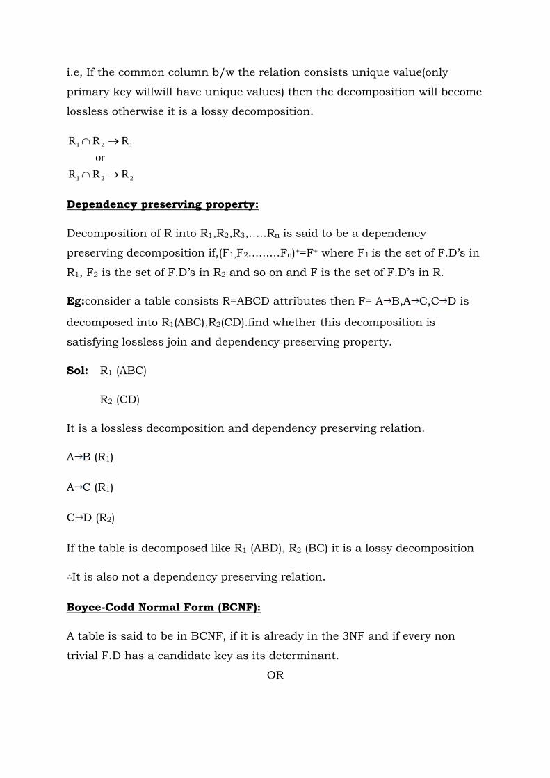
i.e, If the common column b/w the relation consists unique value(only

primary key willwill have unique values) then the decomposition will become

lossless otherwise it is a lossy decomposition.

221

121

RRR

or

RRR

Dependency preserving property:

Decomposition of R into R1,R2,R3,…..Rn is said to be a dependency

preserving decomposition if,(F1,F2.........Fn)+=F+ where F1 is the set of F.D’s in

R1, F2 is the set of F.D’s in R2 and so on and F is the set of F.D’s in R.

Eg:consider a table consists R=ABCD attributes then F= A B,A C,C D is

decomposed into R1(ABC),R2(CD).find whether this decomposition is

satisfying lossless join and dependency preserving property.

Sol: R1 (ABC)

R2 (CD)

It is a lossless decomposition and dependency preserving relation.

A B (R1)

A C (R1)

C D (R2)

If the table is decomposed like R1 (ABD), R2 (BC) it is a lossy decomposition

It is also not a dependency preserving relation.

Boyce-Codd Normal Form (BCNF):

A table is said to be in BCNF, if it is already in the 3NF and if every non

trivial F.D has a candidate key as its determinant.

OR

A table is said to be in BCNF if all determinants are keys in the 3NF table or

they must be super keys

Anomalies can occur in relation in 3NF if there are determinants in

the relation that are not candidate keys.

A relation is in BCNF if every determinant is a candidate key,

To test whether a relation is in BCNF, we identify all the determinants

and make sure that they are candidate key.

The following conditions are not properly handled by 3NF

(1) If table consists two or more composite primary keys

(2) If the candidate keys overlap.

3 NF 2 NF

1.It concentrates on the primary

key

it concentrates on all

candidate keys

2.Redundancy is high compared

to BCNF

Redundancy is low compared

to 3 NF

3.It may preserve all

dependencies

It may not preserve all F.D’s

4.If there is a dependency x y is

allowed in 3NF if x is a super key

or Y is the part of key

If there is a dependency x

y.It is allowed in BCNF if X is

super key.

Q:

(1) R=ABCD

A D

C A

B C

Sol:

(a) Key=b

(b) At present A,B,C,D one in 2NF

(c) BACD

(2)B C

D A

Sol:

(a) Key=BD

(b) 1 NF

(c) 2 NF=BC,DA,BD

3 NF= BC, DA, BD

(d) BCNF= BC,DA,BD

BCDDA

Lossless decomposition.

(3) ABC D

D A

Sol:

(a) Key=ABC,BCD

(b) let key=ABC

3 NF

(c) BCNF=ABC

Super key ABC D

D A

BCD, DA (but ABC will not be a key)

Q. ABCDR

BA

DBC

CA

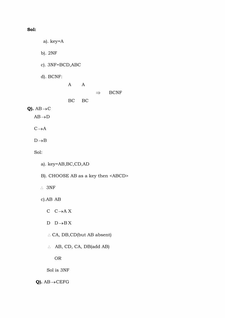
Sol:

a). key=A

b). 2NF

c). 3NF=BCD,ABC

d). BCNF:

A A

BCNF

BC BC

Q). ABC

ABD

CA

DB

Sol:

a). key=AB,BC,CD,AD

B). CHOOSE AB as a key then <ABCD>

3NF

c).AB AB

C CA X

D DB X

CA, DB,CD(but AB absent)

AB, CD, CA, DB(add AB)

OR

Sol is 3NF

Q). ABCEFG

AD

FG

FBH

HBCADEFG

FBCADE

Sol:

a).key = AB,HBC,FBC

B). Choose key AB <ABCDEFGH> AD

ABCEFGH

2NF=AD,ABCEFGH

c). 3NF=AD,ABCEFGH FG

ABCEFH

3NF=AD, FG, ABCE, FH ABCEF

FBH

D).BCNF

AB A

A F

F AB

FB

HBC

FBC

BCNF=FG,AD,FBH,ABCEF

Q). R=ABCD

R1=BC &AD(R2)

(1).

BC

DA

Sol:

(1) a).key=BD

b).R1R2=0

lossy decomposition

bad decomposition

The decomposition is bad decomposition

it is not satisfying lossless join property but it is satisfying

dependency preserving property.

(2).ABC

CA R1=ACD

CD R2=BC

A). key=AB,BC

b). R1R2=C

it is a lossless decomposition as common attribute ’c’ can become a

key for the first table ACD.

(3). A BC R1=ABC

C AD R2=AD

A).KEY=A

b). R1R2=A

It is a lossless decomposition as A is a common attribute and can

become a key.

(4). A B

B C R1=AB

C D R2=ACD

Sol:

a).key= A

b). R1R2=A

Lossless

FD not preserved B C

Q).

A B R1=AB

B C R2=AD

C D R3=CD

Sol:

It is a lossy decomposition

Q).

R=ABCDE

AB DE

A C

D E

Sol:

(a) Key=AB

(b) 2 NF=ABDE,AC

(c) 3 NF=ABD,DE,AC

(d) BCNF=AB AB

D A

D A

Q)

AB CDE

C A

D E

Sol:

(a) Key=AB,BC

(b) choose AB as a key and no partial dependencies

3 NF=ABCD, DE

BCNF= ABCD,CA,DE

Limitations of Normalization:

(1) It cannot detect redundancy among the tables.

(2) It may slow down the query retrival process

(3) The decomposed tables may not have real world meaning i.e, we

cannot understand the significant of the tables straight away.

Solutions:

To avoid all the problems selectively we go for De-Normalization

i.e,decomposed relations are combined together to improve the

performance of the speed up the data retrieval.

Advantages:

(1) Database consistency can be achieved

(2) It increases the speed (By eliminating the duplicates)

(3) It reduces the disk size

(4) It maintains the integrity.

Multi-Valued Dependencies (MVD)

The possible existence of multi-valued dependencies in a relation is due to

first normal form (1NF), which disallows an attribute in a tuple from having

a set of values.

For example, if we have two multi-valued attributes in a relation, we have to

repeat each value of one of the attributes with every value of the other

attribute, to ensure that tuples of a relation are consistent. This type of

constraint is referred to as a multi-valued dependency and results in data

redundancy.

Consider the Employee relation which is not in 1NF shown in figure:

EmpNum EmpPhone EmpDegrees

111

{ 040-222222,

040-333333}

{ BA, BSc}

The result of 1NF on above relation is shown below:

EmpNum EmpPhone EmpDegrees

111 040-222222 BA

111 040-333333 BSc

111 040-222222 BSc

111 040-333333 BA

This relation records the EmpPhone and EmpDegrees details of an employee

111. However, the EmpDegrees of an employee are independent of

EmpPhone. This constraint results in data redundancy and is referred to as

multi-valued dependency.

Multi-Valued Dependency (MVD):

Represents a dependency between attributes (for example, A, B, and C) in a

relation, such that for each value of A there is a set of values for B and a set

of values for C. However, the set of values for B and C are independent of

each other.

We represent an MVD between attributes A, B, and C in a relation using the

following notation:

A →→ B

A →→ C

For example, we specify the MVD in the above Employee relation as follows:

EmpNum →→ EmpPhone

EmpNum →→ EmpDegrees

Formally, an MVD can be defined as:

Let R be a relation schema, and X and Y be disjoint subsets of R, and Z =

R─XY.

If a relation R satisfies X →→Y2, the following must be true for every legal

instance of r of R:

if for any two tuples t1, t2 and t1(X) = t2(X), then there exist t3 in r such

that

t3(X) = t1(X), t3(Y) = t1(Y), t3(Z) = t2(Z).

By symmetry, there exist t4 in r such that, t4(X) = t1(X), t4(Y) = t2(Y), t4(Z) =

t1(Z).

2 X→→Y can be read as X multi-determines Y.

The MVD X→→ Y says that the relationship between X and Y is independent

of the relationship between X and R─ Y.

Armstrong Axioms rules relate to MVDs:

MVD Complementation: If X→→Y, then X→→R─XY.

MVD Augmentation: If X→→Y and W be super set of Z, then

WX→→YZ.

MVD Transitivity: If X→→Y and Y→→Z, then X→→(Z─Y).

Trivial MVD:

An MVD A→→B in relation R is defined as being trivial if,

a) B is a subset of A or

b) A U B = R.

An MVD is said to be non-trivial if neither a) nor b) is satisfied.

Fourth Normal Form (4NF):

A relation that is in Boyce-Codd normal form and contains no non-trivial

MVDs.

X Y Z

x1 y1 z1 t1

x1 y2 z2 t2

x1 y1 z2 t3

x1 y2 z1 t4

Formally, Let R be a relation schema, X and Y be nonempty subsets of the

attributes of R. R is said to be in 4NF, if, for every MVD X→→Y that holds

over R, one of the following is true:

Y is a subset of X or XY = R, or

X is a super key.

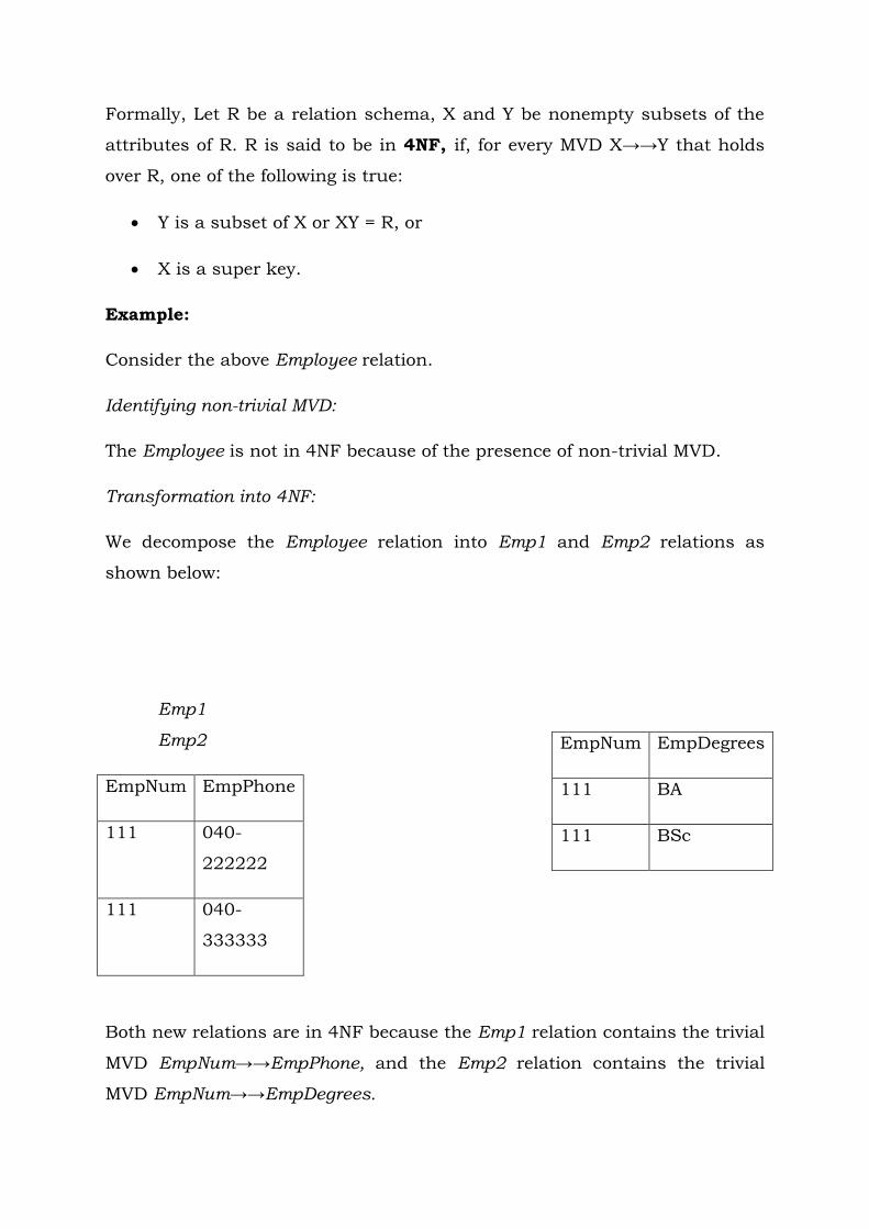
Example:

Consider the above Employee relation.

Identifying non-trivial MVD:

The Employee is not in 4NF because of the presence of non-trivial MVD.

Transformation into 4NF:

We decompose the Employee relation into Emp1 and Emp2 relations as

shown below:

Emp1

Emp2

EmpNum EmpPhone

111 040-

222222

111 040-

333333

Both new relations are in 4NF because the Emp1 relation contains the trivial

MVD EmpNum→→EmpPhone, and the Emp2 relation contains the trivial

MVD EmpNum→→EmpDegrees.

EmpNum EmpDegrees

111 BA

111 BSc

Properties of Decomposition

Lossless-Join Decomposition:

Let R be a relation schema and let F be a set of FDs over R. A decomposition

of R into two schemas with attribute sets X and Y is said to be a lossless-

join decomposition with respect to F if, for every instance r of R that

satisfies the dependencies in F, ∏x (r) ∏y (r) = r. In other words,

we can recover the original relation from the decomposed relations.

From the definition it is easy to see that r is always a subset of natural join

of decomposed relations. If we take projections of a relation and recombine

them using natural join, we typically obtain some tuples that were not in the

original relation.

Example:

By replacing the instance r shown in figure with the instances ∏SP (r) and

∏PD (r), we lose some information.

Instance r ∏SP (r) ∏PD (r)

S P D

s1 p1 d1

s2 p2 d2

s3 p1 d3

S P

s1 p1

s2 p2

s3 p1

P D

p1 d1

p2 d2

p1 d3

S P D

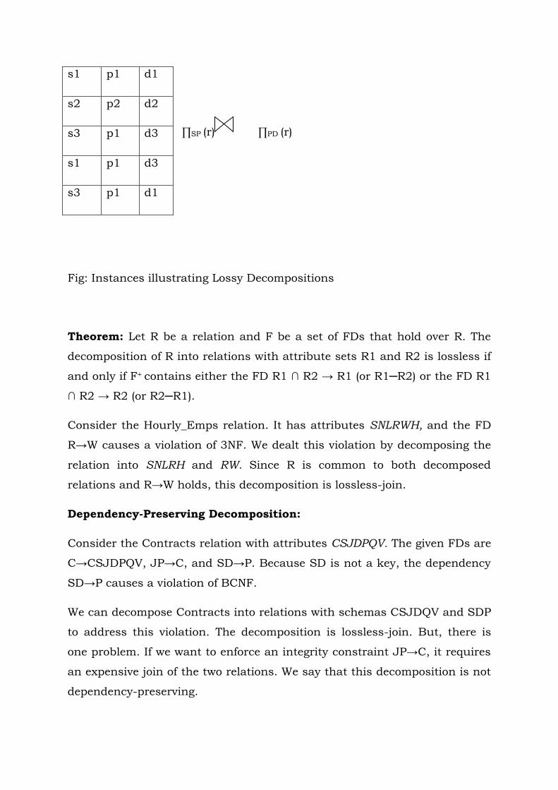
∏SP (r) ∏PD (r)

Fig: Instances illustrating Lossy Decompositions

Theorem: Let R be a relation and F be a set of FDs that hold over R. The

decomposition of R into relations with attribute sets R1 and R2 is lossless if

and only if F+ contains either the FD R1 ∩ R2 → R1 (or R1─R2) or the FD R1

∩ R2 → R2 (or R2─R1).

Consider the Hourly_Emps relation. It has attributes SNLRWH, and the FD

R→W causes a violation of 3NF. We dealt this violation by decomposing the

relation into SNLRH and RW. Since R is common to both decomposed

relations and R→W holds, this decomposition is lossless-join.

Dependency-Preserving Decomposition:

Consider the Contracts relation with attributes CSJDPQV. The given FDs are

C→CSJDPQV, JP→C, and SD→P. Because SD is not a key, the dependency

SD→P causes a violation of BCNF.

We can decompose Contracts into relations with schemas CSJDQV and SDP

to address this violation. The decomposition is lossless-join. But, there is

one problem. If we want to enforce an integrity constraint JP→C, it requires

an expensive join of the two relations. We say that this decomposition is not

dependency-preserving.

s1 p1 d1

s2 p2 d2

s3 p1 d3

s1 p1 d3

s3 p1 d1

Let R be a relation schema that is decomposed into two schemas with

attributes sets X and Y, and let F be a set of FDs over R. The projection of

F on X is the set of FDs in the closure F+ that involve only attributes in X.

We denote the projection of F on attributes X as FX . Note that a dependency

U→V in F+ is in FX only if all the attributes in U and V are in X.

The decomposition of relation schema R with FDs F into schemas with

attribute sets X and Y is dependency-preserving if (FX U FY)+ = F+.

Example:

Consider the relation R with attributes ABC is decomposed into relations

with attributes AB and BC. The set of FDs over R includes A→B, B→C, and

C→A.

The closure of F contains all dependencies in F plus A→C, B→A, and C→B.

Consequently FAB contains

A→B and B→A, and FBC contains B→C and C→B. Therefore, FAB U FBC

contains A→B, B→C, B→A

and C→B. The closure of FAB and FBC now includes C→A (which follows from

C→B and B→A). Thus

the decomposition preserves the dependency C→A.