ISSN 1440-771X

AUSTRALIA

DEPARTMENT OF ECONOMETRICS AND BUSINESS STATISTICS

Reconstructing the Kalman Filter for Stationary and Non Stationary Time series

Ralph D. Snyder and Catherine S. Forbes

Working Paper 14/2002

1

Reconstructing the Kalman Filter for Stationary and Non Stationary Time Series

JOINT WORKING PAPER WITH THE DEPARTMENT OF ECONOMETRICS & BUSINESS STATISTICS AND THE BUSINESS AND ECONOMIC FORECASTING UNIT.

October 2002

Ralph D. Snyder

Department of Econometrics and Business Statistics

Monash University

Clayton, Victoria 3185

Australia

(613) 9905 2366

ralph.snyder@buseco.monash.edu.au

Catherine S. Forbes

Department of Econometrics and Business Statistics

Monash University

Clayton, Victoria 3185

Australia

(613) 9905 2471

catherine.forbes@buseco.monash.edu.au

2

Reconstructing the Kalman Filter

Abstract

A Kalman filter, suitable for application to a stationary or a non-stationary time

series, is proposed. It works on time series with missing values. It can be used on

seasonal time series where the associated state space model may not satisfy the

traditional observability condition.

A new concept called an ‘extended normal random vector’ is introduced and used

throughout the paper to simplify the specification of the Kalman filter. It is an

aggregate of means, variances, covariances and other information needed to define

the state of a system at a given point in time. By working with this aggregate, the

algorithm is specified without direct recourse to those relatively complex formulae

for calculating associated means and variances, normally found in traditional

expositions of the Kalman filter.

A computer implementation of the algorithm is also described where the extended

normal random vector is treated as an object; the operations of addition, subtraction

and multiplication are overloaded to work on instances of this object; and a form of

statistical conditioning is implemented as an operator.

Keywords

Time series analysis, forecasting, Kalman filter, state space models, object-oriented programming.

JEL: C13, C22, C44

3

1. Introduction Being the cornerstone of modern programming practice, objects and classes provide a useful

basis for structuring computer code. They promote data aggregation based on concepts

inherent in applications. They lead to simplified code that is usually easier to understand and

to maintain.

Being a systematic way of thinking about problems and the contexts in which they occur, it is

our contention that the object-oriented approach transcends computer programming in its

usefulness. The purpose of this paper is to demonstrate that the approach can promote useful

ways of thinking in statistical theory. We illustrate this point by treating normal random

vectors as objects and applying them to the problem of filtering time series.

More specifically, data-aggregation possibilities associated with an object-oriented approach

are exploited, to simplify the specification of the Kalman filter (Kalman, 1960; Kalman and

Bucy, 1961). The mean and variance of a random vector are combined into a single structure.

Operations of addition, multiplication and conditioning are defined on instances of this

structure. Then the Kalman filter, for stationary time series, is defined in terms of the

resulting object and its operations.

This normal random vector object is then extended to include a special matrix required in the

case of non-stationary time series to carry additional information forward through time. This

extended normal random vector object is used to specify a new augmented Kalman filter for

non-stationary time series, one that has a more concise specification than existing approaches

and one that avoids certain limitations, outlined later in the paper, of its closest antecedent:

the approach of Harvey (1991).

4

The Kalman filter (Kalman, 1960, Kalman and Bucy, 1961) is essentially an algorithm for

revising the moments of stochastic components of a linear time series model to reflect

information about them contained in time series data. It is often used as a stepping-stone to

deriving the moments of components at future points of time for forecasting purposes. It is

useable in real time applications, because revisions to the moments are made recursively as

each successive member of a time series is observed. It can also be used as part of the

process required to find maximum likelihood estimates of unknown model parameters

(Schweppe, 1965; Harvey, 1991). It is therefore generally perceived as having a central role

in modern time series analysis.

The equations in the Kalman filter for calculating the required means and variances were

originally derived using projection theory in linear spaces. Duncan and Horn (1972), who

sought to simplify matters for those unfamiliar with this theory, showed that the equations

could be derived using a stochastic coefficients regression framework. Meinhold and

Singpurwalla (1983), with a similar quest, employed the theory of conditional probability.

Both approaches simplified the derivation of the Kalman filter equations. They did not,

however, simplify the form of these equations.

The plan of this paper is as follows. A condensed version of the linear state space model is

introduced in Section 2. An outline of a general filter is presented in Section 3. The new

object and associated operations are defined in Section 4. The reconstructed Kalman filter for

stationary time series is presented in Section 5. An extension to the object to handle division

by singular matrices is detailed in Section 6. The augmented Kalman filter for non-stationary

time series is considered in Section 7. Finally, the role of the algebraic system in facilitating a

logical structure for an object-oriented computer implementation of the Kalman filter is

outlined in Section 8. Throughout the paper, all random vectors are governed by a multi-

variate normal distribution. The term ‘normal random vector’ is abbreviated to NRV.

2. Linear Statistical Model: Dynamic Form

The key problem of time series analysis is to account for inter-temporal dependencies. A

common practice is to rely on a mix of observable and unobservable quantities that are

understood to summarise the state of a process under consideration at a given point of time

and to specify how they change over time. Traditionally, the distinction between observable

and unobservable quantities is preserved with the use of two symbols. In our quest to

minimize notation we combine them into a single random vector, which at typical time t, is

designated by � �x t�

. The problem of distinguishing between both types of quantities will be

considered later in the exposition. Note that, throughout the paper, a tilde is used to indicate

that the associated quantity is random.

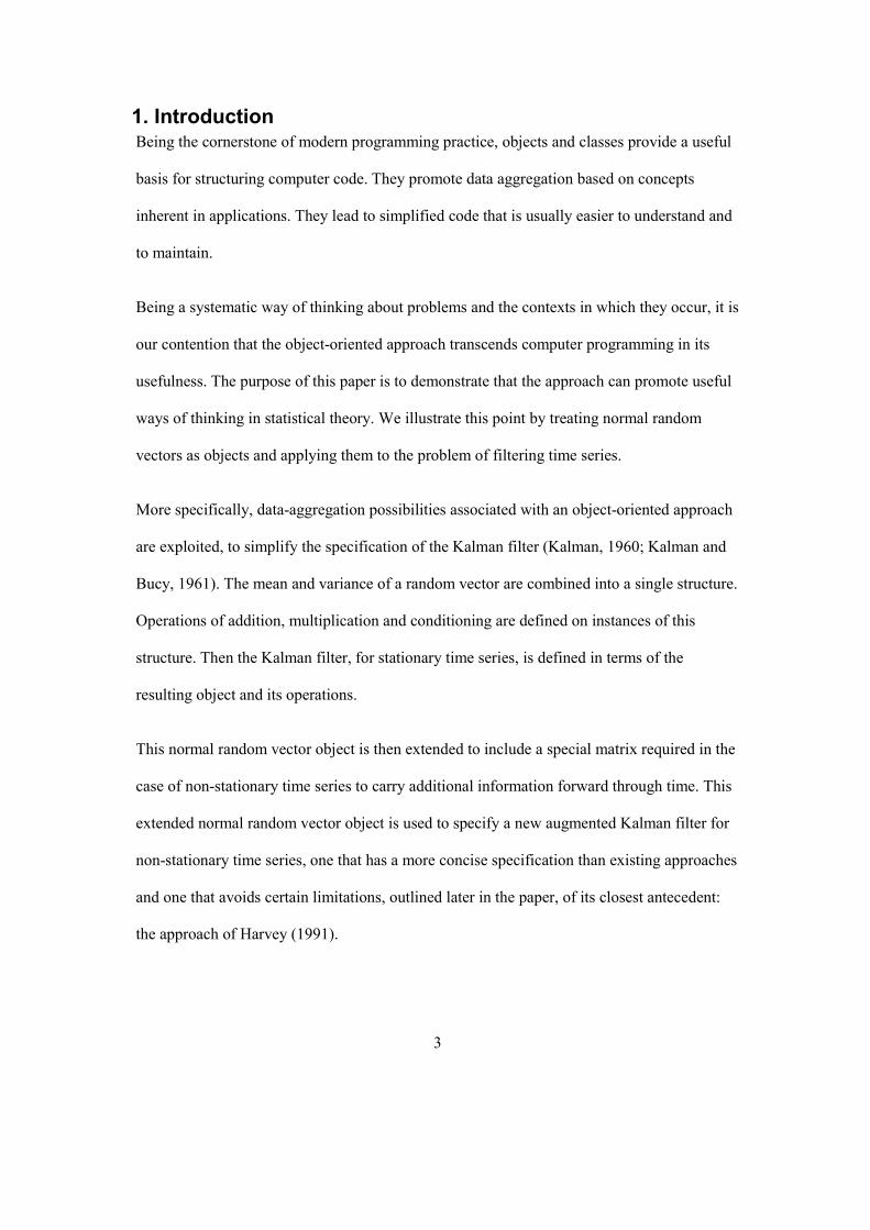
The inter-temporal dependencies are captured by the first-order recurrence relationship

� � � � � �1x t Ax t u t� � �

� � �. (2.1)

A is a fixed matrix. The random vector � �u t�

represents the effect of concurrent factors on

the process. This random vector is assumed to have a zero mean and a constant variance

matrix. The � �u t�

are serially uncorrelated. To reduce notational complexity, the scope of the

paper is restricted to the invariant case of the so-called state space model. Invariant state

space models are the most commonly used in practice. Moreover, what follows is easily

generalised with the use of further time subscripts.

5

The recurrence relationship (2.1) must be provided with a seed. It is therefore also assumed

that

� �0x x�� �

(2.2)

where x�

is a random vector with a known probability distribution. It will be seen that for

non-stationary series, the distribution of x�

may not be completely known, in which case

special measures must be taken to accommodate this more challenging case. Either way, it is

further assumed that the � �u t�

are uncorrelated with x�

.

Example 2.1

The local level model (Muth, 1960) is a common special case. It underlies simple exponential

smoothing, a widely used method for forecasting inventory demand (Brown, 1959). The

series values � �z t�

are randomly scattered about a path traced by a wandering level � �t� .

More specifically

� � � � � �

� � � � � �1

2

11

z t t ut t u� � �

� � �

�� � �� �� � �

tt

This model can be rewritten in conformity with (2.1) as

� �

� �

� �

� �

� �

� �1

2

10 110 1

z t z t ut t

�� � � � �� �� �� � � � �� � �� � � �

� � �� �� �

tu t

��

� .

Note that the component vector consists of the observable quantity � �z t�

and the

unobservable quantity � �t�� .

6

3. Filtering Time Series

The state space model may be used, in conjunction with past data, to generate forecasts. A

vector � �x t without the tilde represents the observed value of the typical random

components vector � �x t�

. In the case of vector auto-regressions, all the elements of the

observation vector � �x t are typically known (Lütkepohl, 1991). In models with unobserved

components, however, the unobserved parts of � �x t may be treated as missing values. Thus,

in the local level example, an observation is represented by � � � � , #x t z t� � � �� � where

designates a ‘missing value’.

#

The forecasting problem is to derive the distributions of future components vectors using

information from a sample of size n. It may be expressed more formally by introducing the

notation � �,x t s�

to represent the random vector � �x t�

once its distribution has been revised

with all the observations from periods 1 to s. The possibilities for � �,x t s�

are depicted in

Figure 1 for different values of s and t. In particular, the forecasting problem can be

expressed as one of deriving the distributions of � �,x n j n��

where j designates the

prediction lead-time index.

7

Figure 1. Difference between filtered and smoothed components vectors.

The required future prediction distributions are related to the distribution of the final

components vector � �,x n n�

. Once the moments of the latter are known, the moments of the

prediction distributions can be generated from appropriate recursive relationships implied by

(2.1). Thus, the quest reduces to finding the distribution of the final components vector.

Two paths, depicted in Figure 1, may be followed in the derivation of the distribution of

� �,x n n�

. The first, based on the approach of Duncan and Horn (1972), converts the dynamic

linear model (2.1) into an equivalent random coefficients regression model. The unknown

components are treated as the random coefficients. The known components are regarded as

the observations of a dependent variable. The regression is fitted to the entire sample of size

n to yield the moments of the random vectors depicted in the final column of Figure 1.

This regression approach is rarely used in practice. The associated data matrix is normally

quite large and this is commonly perceived as a hindrance to efficient computation. Thus, a

second approach may be used that effectively follows the diagonal path depicted by the

8

arrows in Figure 1. At the beginning of typical period t, the moments of � �, 1x t t ��

are

calculated from the moments of the previous � �1, 1x t t� �

� using the moments equations

implied by (2.1). At the end of typical period t, the random vector � �, 1t �x t�

is revised with

the observation � �x t to give � �,x t t�

. An algorithm used to implement this type of strategy is

usually referred to as a filter. It may be summarized by the equations:

Initialisation

� �0,0x x�

� � (3.1)

For successive periods t = 1, 2,…, n apply the following steps:

Time Advance Step

� � � � � �, 1 1, 1x t t Ax t t u t� � � � �

� � � (3.2)

Revision Step

� � � � � �, , 1 |x t t x t t x t� �

� �. (3.3)

Note that the equation (3.2) is obtained by conditioning (2.1) on � � � � � �1 , 2 , 1x x x t �� . The

equation (3.3) is obtained from a straightforward application of conditioning.

The equations (3.1)-(3.3) provide an overview of filtering. More details, however, must be

elaborated, before these equations become operational. In particular, they imply relationships

for calculating the moments of the associated random variables. It is one version of these

relationships that form the so-called Kalman filter.

9

In a sense, the equations for the Kalman filter are redundant. The filtering equations (3.2) and

(3.3) involve addition (+), multiplication by a fixed matrix and conditioning (|). If the impact

of these operations on the moments of normally distributed random vectors is defined in

general, then the equations (3.2) and (3.3) suffice to describe how the pertinent moments can

be calculated without recourse to further equations specific to the filtering context. This

strategy leads to an algebraic system for Gaussian random vectors.

4. An Algebraic System for Gaussian Random Vectors

In this paper, the notation � �,x xN V� is used to represent an NRV x�

. It enables us to

highlight the dependence of the NRV on its mean and its variance V . Given this

convention, it is legitimate to write

x� x

� �x,xx N �� V�

. Note that any constant vector x can be

written as � �,0N x .

This notation provides a means for succinctly defining operations on NRVs. More

specifically, if x�

and are uncorrelated NRVs, then y�

� �,x y x yx y N V V� �� � � �

� �

(4.1)

� �,x y x yx y N V V� �� � � �

� �

. (4.2)

If A is a fixed matrix, then

� �,x xAx N A AV A� ���

. (4.3)

Furthermore, if A is a square, non-singular matrix, then

10

� �1 1\ ,x xA x N A A V A�� � �

���

1 . (4.4)

The notation, in conjunction with these definitions, admits the possibility of more compact

representations of equations involving moments of NRVs. It is now possible to write

z x y� �

� � �

instead of the two equations z x� � �� � y and z x yV� �V V ; z x y� �

� � �

instead

of z x �� � y� � and z x yV� �V V ; y Ax�

��

in place of the equations y xA��� and

. Note that the distributive law yV AV� x A� � �A B x� � Ax Bx�

� � � applies.

Conditioning is another important operation. It is established in the Appendix that |x x�

is a

weighted average of x�

and x . More specifically,

� �|x x I W x W� � �

� �x (4.5)

where I is an identity matrix and W a ‘weight’ matrix. In the special case where x contains no

missing values, we require that |x x x�

�. This is achieved when W . At the other

extreme, when all the elements of x are missing values, no revision is needed. In other words

I�

|x x x�

� �, a situation obtained when W In the most common case, where x is a partial

observation, the task of finding

0.�

|x x�

is broken into a succession of smaller transformations of

the same form, one for each observed element in x. In the typical case, where the element px

of the k-vector x is a genuine observation, the following steps are applied. First, construct a

‘weight’ matrix pW using the rule

p x p p p x pW V e e e V e� �� (4.6)

11

where pe is the unit coordinate vector with its pth element equal to 1. Second, obtain a

revised value of x�

using the generalised weighted average � �p pI W x W x� �

�.

The definitions of the + and – operators in 4.1 and 4.2 have been restricted to uncorrelated

NRVs. The framework can indirectly accommodate correlated NRVs by stacking them.

Thus, if 1x�

and 2x�

are two correlated random vectors, their sum can be found by stacking

them and then finding the product � � 1

2

xI I

x� �� �� ��

�

where I is a commensurate identity matrix.

Since 1x�

and 2x�

only contain information on variances, covariance information would have

to be incorporated separately into the stacking process. A stacking function like

� �1 2 , 12stack ,x x x V�

� � �, where V is the covariance matrix, would be required in any

computer implementation.

12

5. The Kalman Filter

Using the operations from Section 4, the equations (3.2) and (3.3) now fully define how the

moments of the state vectors are revised over time. These equations are therefore a very

compact representation of the Kalman filter. Compactness is achieved because:

The observed and unobserved components are combined into a single vector.

The state space model consists of only one equation instead of the more usual measurement

and transition equations.

Means and variances are combined into a single entity so that the way they are calculated is

described by a single equation.

12

It should be emphasised that all we have done so far is to repackage the Kalman filter. The

reduction in notation and equations simplifies its specification. It does not, however, reduce

computational loads. Depending on how it is implemented, computational loads stay about

the same.

6. An Extension to the Algebraic System of NRVs

The division operation defined by (4.4) presumed the non-singularity of the matrix A. The

focus of this section is on what happens when A is potentially singular. The theory of NRVs

is extended to accommodate generalised inverses.

When A is singular, the Moore-Penrose generalised-inverse is represented by and

satisfies the condition . The general solution of the equation is

A�

bAA A A�

� Ax �

� �x A b I A A�

� � � ��

Ax b�

� �

where � is an arbitrary vector. When extended to the space of

NRVs, the equation has a general solution � �x A b I A A�

� � � ��

� � � where � is a

Gaussian random vector with arbitrary variances.

�

To obtain a properly integrated algebraic system of NRVs that accommodates division by

singular matrices, the typical NRV x�

is extended to a new object designated by *x�

that is

defined by *xx x B �� �

� � � where xB is a fixed matrix. It is inconvenient to carry the �

notation, so

�

*x�

is represented by � �, ,x x xN V B� , the ��

now being implicit. We call *x�

an

extended normal random vector (ENRV). Note that an NRV is a special case of an ENRV

where . A constant vector is a special case where, in addition, V . 0�xB 0x �

13

Suppose that *xx x B �� �

� � � and *

yy y B �� �

�� �

and that x�

and y�

are uncorrelated. Note that

*x�

and cannot be uncorrelated because of their mutual dependence on � . However, for

any given value � of � , both

*y� �

�

*x�

*y and �

are then uncorrelated. We say that *x�

and are

conditionally uncorrelated.

*y�

The random vector operators are extended as follows. First, if *x�

and *y�

are conditionally

uncorrelated ENRVs, then the ‘plus’ and ‘minus’ operations are defined by

� �* * , ,x y x y x yx y N V V B B� �� � � � �

� �

(6.1)

� �* * , ,x y x y x yx y N V V B B� �� � � � �

� �

. (6.2)

For a fixed matrix A and an ENRV *x�

, the definition of the ‘times’ operator is extended to:

� �* , ,x x xAx N A AV A AB� ���

. (6.3)

‘Division’ is defined in terms of generalised inverses as

� � � �*\ , ,x x xA x N A A V A I A A A B�� � � � �

� ��� �� � �

� (6.4)

The latter arises because � �* *\A x A x I A A �� �

� � �

� � �. Substituting *

xx x B �� �

� � � this

becomes � �xA B I A A� �� � �

� �

� �

*\A x A x� �

� �.

Conditioning with extended NRVs involves added complexity because of the arbitrary

component. This is illustrated by the following example.

14

Example 6.1

Suppose that and * 10 8 2 2 0, ,

5 2 30 5 0x N

� �� � � � � �� � � � �

� � �� ��

20#

x� �

� � �� �

. Clearly,

where u is a Gaussian random variable with mean 0 and variance 8. Now let and

solve for � to get �

1

*1 110 2x u �� � �

� �

1 20x �

�

1�

1�

1 15 0.5u� �

� �. The second equation is

2

*x 25 u� � � 15�� � �

2

1�

where u is a

Gaussian random variable with mean 0 and variance 16. On the elimination of � , it becomes

*2 30 1 22.5x u u� � �

20 0 0 0 0| , ,

30 0 60 0 0� �� � � � � �� � � � � � ��

x

� �

2

�

. The dependence on the arbitrary vector � is then broken. Noting that

and u are correlated, it can be shown from these equations that

. In effect, Gaussian elimination has been used to

reduce the first column of the

1

1u

*x x�

N �

B to a null vector, so destroying the dependence of *x�

on any

arbitrary random vector.

More generally, if x is an observation of *x�

, possibly containing missing values, then

� � � � � � � �� �* | , ,x x xx x N I W Wx I W V I W I W B��

� � � � � ��

(6.5)

where W is a ‘weight’ matrix chosen to annihilate columns of xB associated with the

arbitrary random vector and to annihilate missing values in x . The transformation (6.5) is

broken down into a sequence of smaller transformations of a similar form applied for each

successive observed value in x. In the typical case, where the element px of x is a genuine

observation, the following steps are applied:

15

Case 1 (row p of xB is null)

Apply the conventional conditioning update by constructing a ‘weight’ matrix pW using the

rule:

p x p p p x pW V e e e V e� �� . (6.6)

Case 2 (the qth element in row p of xB is non-zero)

Construct the weight matrix so that it can eliminate the arbitrary random variable � : q

p x q p p x qW B e e e B e� �� . (6.7)

In both cases the revised *x�

is obtained with � � *p pI W x W x� �

�.

The rationale for (6.6) is given in the Appendix. The effect of the transformation (6.7) is to

eliminate the qth column x qB e of xB because � � 0p x qI W B e� � .

Example 6.2

Example 6.1 began with , V105x�

� �� � �� �

8 22 20x� �

� � �� �

and 2 05 0xB� �

� � �� �

. Thus, by (6.7)

� � � �1

2 0 1 01 0

5 0 0 0W

� � � �� � � �� � � �

21 0

5�

� ��

0 1 10 0 2.5� � � �� � � �� � � �

�� �

�1I W and

0 02.5 1

� �� � � ��� �

. Using

(6.5), the revised quantities are:

16

17

�� �

�

���

���

new 0 0 10 1 0 20 202.5 1 5 2.5 0 # 30x�

� � � � � � � � �� � � � � � � � � ��� � � � � � � � �

new 0 0 8 2 0 2.5 0 02.5 1 2 20 0 1 0 60x

V�� � � � � � �

� �� � � � � � ��� � � � � � �

new 0 0 2 0 0 02.5 1 5 0 0 0xB

� � � � �� �� � � � ��� � � � �

.

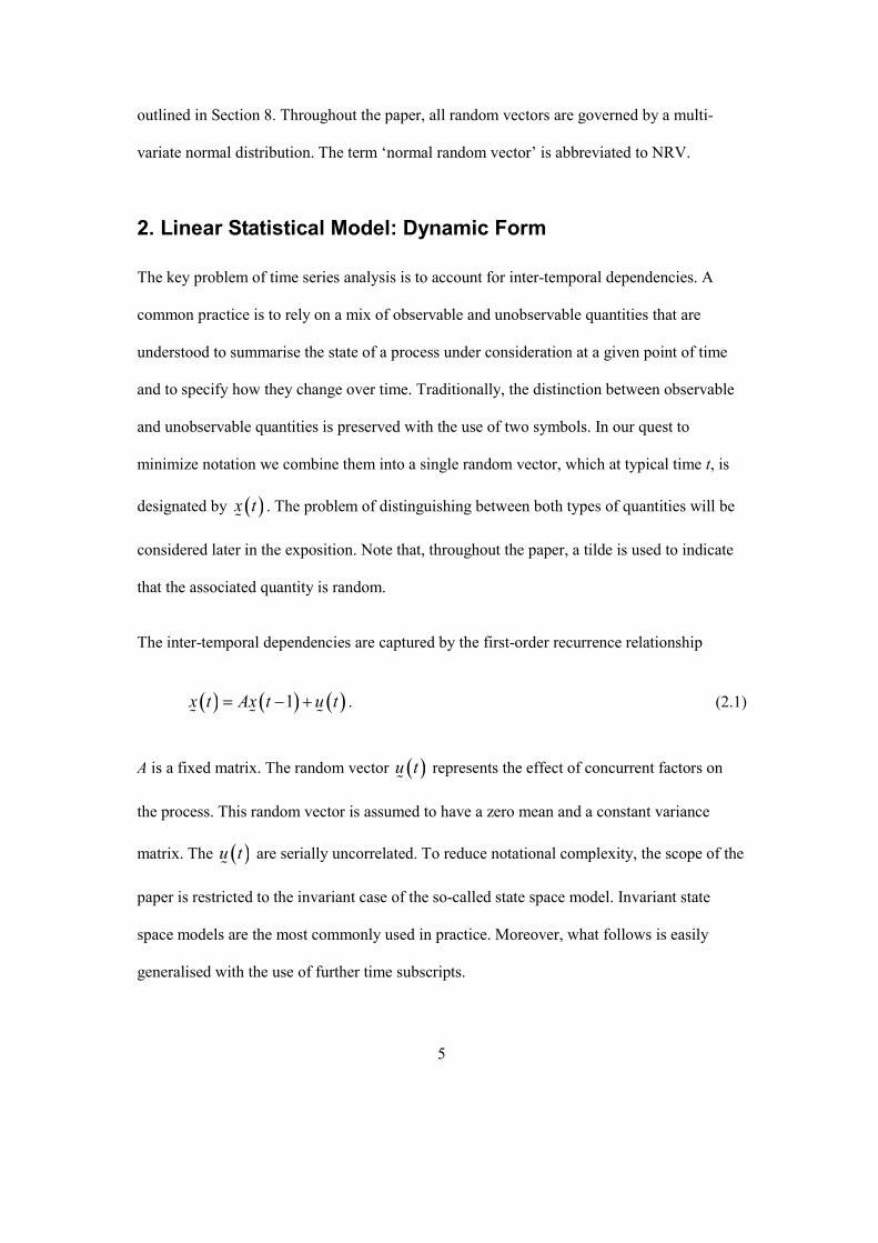
These results are exactly the same as those obtained by the substitution method in Example

6.1. As before, the effect of the transformation has been to drive the remaining non-zero

column of xB to a null vector, ensuring that the new components vector does not depend on

the undefined random vector � . The transformation has also annihilated the missing value,

designated by #, in the observation vector.

�

7. Filtering Non-Stationary Time Series

Equation (3.1), which describes the initialisation of the Kalman filter, requires knowledge of

the moments of � �0x x�

� �. If the time series under consideration is stationary, then x

� has a

mean of zero and its variance satisfies the steady state equation

x xV AV A V�� � u . (7.1)

A method for solving this linear equation is described in Harvey (1991) for stationary time

series. In the stationary case the mean and variance are both completely known so that

. 0xB �

Most time series in business and economic applications are non-stationary, in which case the

transition matrices possess unit eigenvalues. The steady state equation (7.1) then has no

unique solution.

Example 7.1

The damped local trend model is defined by

� � � � � � � �

� � � � � � �

� � � � � �

�

� � � �

1

2

3

2

1 1

1 1

1

~ NID 0, 1, 2,3j j

z t t b t u

t t b t u

b t b t u t

u t j

�

�

� � � � �

� � � � �

� � �

�

�� � � �

� �� � � �

� � �

t

t. (7.2)

The notation is essentially the same as that used in Example 2.1. However, � �b t�

is a growth

rate and � is a damping parameter satisfying the condition . 0 1�� �

This model provides the framework for an approach to forecasting similar to damped

exponential smoothing (Gardner, 1985). The growth rates � �b t form a stationary series with

a steady state distribution � �� �23N 0, 1� �� 2 . The series formed by the levels � �t�

�,

however, is non-stationary. The variance of � �t

� 0 0�

� is arbitrarily large. The consequence is that

the distribution of the seed vector � �x z� � � b � �0 ��� �� �

is only partially defined.

More generally, it is clear that the seed vector must be an ENRV rather than an NRV. Thus,

for example, the NRVs shown in the state space model (2.1) then become ENRVs. The same

thing happens to the NRVs in the Kalman filter specified in section 3. Instead of restating

18

these equations using asterisks to connote the ENRVs, we drop the asterisk on the

understanding that quantities like � �x t�

now designate ENRVs rather than NRVs.

The fact that some elements of a seed vector x�

possess arbitrary marginal distributions does

not preclude the possibility that they have well-defined distributions after they are

conditioned on successive values of � �z t . The extended algebraic system for ENRV’s

provides a systematic framework for implementing this conditioning process. Quite

remarkably, no changes to the specification of the Kalman filter in (3.2) and (3.3) are

required. All the required changes are made at the more basic level of the ENRV object.

The way this extended version of the Kalman filter is initialised depends on the type of

model under consideration. In the stationary case, where the steady state moments of the

components vector are completely defined, the seed is � �0, ,0xx V�

�. At the opposite

extreme, in the non-stationary case where no components have a steady state distribution, the

seed is � �0,0,x I�

�. In the partially defined case of the damped local trend example

� � � �

� � � �

2 2 2 2 23 1 3

2 2 2 23 3

1 0 10 00 , 0 0 0 , 0 1 00 01 0 1

x

� � � � �

� � � �

� �� �� � �� � � �� � � �� � � � �� �� � � � �

�

1 0

0 0.

Another important insight into the operation of this modified version of the Kalman filter

may be obtained by considering the following model.

Example 7.2

A model that contains a trend and seasonal effects takes the form

19

20

�� � � � � � � � �

� � � � � � � �

� � � � � �

� � � � � �

1

2

3

4

1 1

1 1

1

z t t b t c t m u

t t b t u t

b t b t u t

c t c t m u t

� � � � � � �

� � � � �

� � �

� � �

�� � � � �

� �� � � �

� � �

� � �

t

where m designates the number of seasons per year and � �c t�

is the seasonal effect

associated with period t. This model has a lag m . It can be converted to first-order form

to yield, in the case of a quarterly time series:

1�

� �

� �

� �

� �

� �

� �

� �

� �

� �

� �

� �

� �

� �

� �

� �

� �

� �

� �

1

2

3

4

10 1 1 0 0 0 010 1 1 0 0 0 010 0 1 0 0 0 010 0 0 0 0 0 1

1 20 0 0 1 0 0 0 02 30 0 0 0 1 0 03 40 0 0 0 0 1 0

z t z t u tt t u t

b t b t u tc t c t u t

c t c tc t c tc t c t

�� � � �� �� � � �� � �� � � �� �� � � �� � �� � � �� �

� �� � � �� �� � � �� �� �� � � �� �

� �� � � �� �� � � �� �� �� � � �� � �

� � �� �� � �

� � �

� � �

� �

� �

� �

00

�

� �� �� �� �� �� �� �� �� �� ��

.

This example underlies the additive Holt-Winters method of forecasting (Winters, 1960).

When the extended Kalman filter is applied to most time series, the arbitrary random

variables are eliminated after a few iterations. However, in Example 7.2, a form of linear

dependence exists between the level and the seasonal effects. The traditional observability

condition is not satisfied. A consequence is that one of the arbitrary random variables is

never eliminated as the algorithm progresses.

A closer study of this phenomenon indicates that the level and the seasonal effects, in any

period, depend on this residual arbitrary random variable, but the growth rate does not. It

transpires that the coefficients of this arbitrary random variable in the linear equations that

describe these relationships for the level and seasonal effects are always of equal magnitude,

but have opposite sign. Using � as a generic symbol for all those terms in a relationship that

do not depend on a residual arbitrary random variable, an example of the relationships is

� � 1, 0.1t t ��� �� �

� and � � 10.1s t �� � � �3, t �� �

� � � �, 3, 0.1t t t t� �

. Then,

. The offending arbitrary

random variable disappears. This illustrates the point that the prediction distributions of the

� � � �1, ,z t t t t� �

� �

�

1 10.1b � �� � � � �

� �s��

� �� � �

�z t are well defined, although the prediction distributions of the level and seasonal effects

are never properly defined.

A common way of obtaining well-defined distributions of the level and seasonal effects is to

impose the condition that the seed seasonal effects sum to zero. This provides the extra

equation required to solve for the offending artificial variable and to eliminate it from

subsequent expressions for the level and seasonal effects. The problem with this approach is

that subsequent seasonal effects fail to satisfy the ‘sum to zero’ condition. In our view, a

more sensible strategy is not to impose the condition on the seed seasonal effects. The fact

that the linear dependency then persists at any point of time, suggests that it is legitimate to

apply this condition to the output of the Kalman filter at any point of time. When this is done,

the ‘adjusted’ seasonal effects always sum to zero. In order for this strategy to succeed, the

adjusted seasonal effects and corresponding level should never be fed back into the Kalman

filter itself.

To compare the proposed filter with its antecedents, the state space model (2.1) is partitioned

into a measurement equation

� � � � � �1 12 2 11x t A x t u t� � �

� � � (7.3)

21

and transition equation

� � � � � �2 22 2 21x t A x t u t� � �

� � � (7.4)

where � �1x t�

consists of the observable quantities and � �2x t�

consists of the unobservable

quantities. Note that it has been assumed that and to get a model that more

or less conforms to those used in earlier work. To expedite matters it is assumed that

11 0A � 21A 0�

� �1x t�

is

scalar.

Harvey (1991, section 3.3.4) provides one possible solution to the initialisation problem. He

assumes that

the state space model satisfies the observability conditions;

none of the observed values of � � � �1 11 , ,x x k�� �

are missing.

Initially, he considers the case where all k elements of the seed vector � �2 0x have arbitrary

distributions. By progressively applying (2.1), the observable series values � � � �1 11 , ,x x k�� �

can be expressed as linear functions of the seed vector � �2 0x�

. His approach is to substitute

the observed values � � � �1 11 , ,x x k� of these quantities into these relationships to yield k

linear equations in the k unknown seed variables. The observability condition ensures that

these equations are non-singular. Thus, his method involves finding the solution to these

equations and using it to seed the conventional Kalman filter. An adaptation of this approach

to handle the case where the seed state vector is partially informative is then considered.

22

Harvey’s method is predicated on assumptions (1) and (2) above. Since these assumptions

can be violated in practice, his approach needs further adaptation before it can be used for a

general-purpose implementation of the Kalman filter.

Another approach by de Jong (1991) can be restated in terms of ENRVs. It can then be seen

to be quite similar to our filter, the primary difference being that the Gaussian elimination

rule (6.7) is never used. Thus, in the run-in phase, the elements of the arbitrary random vector

do not progressively disappear from the equations. All pertinent quantities remain linear

functions of � . In particular, the observable quantities form a generalised linear regression,

the elements of � being the regression coefficients. Additional equations are used to

progressively calculate the ‘ ’ matrix of the regression. On reaching that point where

this weighted cross-product matrix becomes non-singular, the least-squares calculations are

invoked, the results being used to eliminate �

��

�

1X V X�

�

�. From this point onwards, his approach reverts

to a conventional Kalman filter.

Ansley and Kohn (1985) provide yet another solution to the problem of filtering non-

stationary time series. Koopman and Durbin (2000) recently proposed an algorithm in the

same genre. These algorithms focus on the variance matrices of the state vectors, assuming

that they can be written in the form � � � � �1 0 0 1x xV V� � ��� where � is an arbitrarily large

number and � �0 1 � is a function that converges to zero as � tends to infinity. It is possible

to re-define an ENRV by . In effect the role of the � � � �� 0 1, ,x x xx V V��

�� xB matrix is replaced

by the V . Multiplication is now defined by � �1x

� � � �� �1xAx A A��

0, ,Ax xAV AV� �

�. The details of

their algorithms are eschewed here. In the final analysis, however, we believe that their

23

24

approaches will involve higher computational loads. The redefined form of multiplication

alone involves more operations than (6.3).

When the emphasis is on computational stability, square-root filters (Kaminsky, Bryson, and

Schmidt, 1971) are preferred to the Kalman filter. A square-root filter in Snyder and Saligari

(1996) is particularly pertinent in our context. It relies on fast Givens transformations to

preserve the triangular structure of the square-root variance matrices. It was shown that the

fast Givens transformations collapse to conventional Gaussian elimination during the run-in

phase. It is this result that provides the rationale for our use of Gaussian elimination in

section 6.

8. Computer Implementation: An Object Oriented Approach

The form of the algorithm, as outlined in this paper, was conceived while implementing the

Kalman filter using the matrix-oriented computer programming language Matlab

(www.mathworks.com). The facilities for object-oriented programming in this language

provided an opportunity to explore data aggregation possibilities. The concept of an NRV

object arose as a result.

A structured array is used to represent a NRV object in the implementation. It has three fields

containing the mean, variance and the matrix of coefficients for the artificial components.

The notation used is kept as close as possible to the mathematical notation. Thus xtilde

designates an NRV object. Its properties are designated by xtilde.mu, xtilde.V and xtilde.B.

The standard Matlab operators +, * and | are overloaded to work on moments-objects.

Function xtilde =KalmanFilter(x, A, utilde, xtilde0);

xtilde = xtilde0;

For t = 1:size(x,2);

xtilde = A* xtilde + utilde;

xtilde = xtilde | x(:,t);

End;

Figure 2. Kalman Filter

The code for the Kalman filter, based on the equations (3.1), (3.2) and(3.3), is shown in

Figure 2. It is relies on inputs utilde and xtilde0 for the disturbance and seed state vectors.

These particular inputs are created outside the Kalman filter function using one of the

variations of the polymorphic constructor function N shown in Table 1. The details of the

code for this constructor function are eschewed in the interests of saving space. Data, to be

filtered, is fed to the function through the k matrix x. Elements of x corresponding to

unobserved components are treated as missing values. They are designated in Matlab using

the not-a-number notation NaN. The output, xtilde, represents

n�

� �,x n n�

.

xtilde = N(mu, V) Creates a NRV object from a specified mean vector and variance matrix. The component B = 0.

xtilde = N (mu, V, B) Creates an ENRV object.

xtilde = N (x) Converts a vector to its equivalent ENRV object with a zero variance. Missing values are reflected in the B matrix.

ytilde = N (xtilde) Creates an ENRV object ytilde equal to the ENRV object xtilde.

Table 1. Forms of the N Constructor Function

25

26

On encountering the + operator between two NRV objects in the code, Matlab automatically

invokes the plus function shown in Figure 3. This function is also polymorphic because it

allows the inputs to be NRVs or fixed vectors. Any fixed vector is converted to its random

vector object counterpart in the first two lines of the body of the function.

Similarly, when * is encountered in a statement between a fixed matrix A and a random

vector object xtilde, a function called ‘times’, based on the definition (6.3), is invoked. The

code for this operator is a relatively simple adaptation of the function shown in Figure 3.

function y = plus(x1, x2);

x1 = N(x1);

x2 = N(x2);

y = N (x1.mu + x2.mu, x1.V + x2.V, x1.B + x2.B);

Figure 3. Code for the overloaded + operator.

Matters are more complex for the conditioning operator |. Matlab normally employs the

symbol ‘|’ to represent the logical operator ‘or’. But this operator is overloaded and given a

completely new interpretation by creating a function called ‘or’ based on the conditioning

rules associated with (6.5). On encountering a statement such as ytilde = xtilde | x, Matlab

inspects the term on the left of the | operator. If this term is a random vector object it calls the

new function, and despite its name, applies the conditioning rules contained within it.

The functions ‘N, ‘plus’, ‘times’ and ‘or’ are placed in files called N.m, plus.m, times.m and

or.m respectively. These files are in turn placed in a folder called @N. The @ symbol is

required by Matlab to designate folders that contain the functions defining objects. The string

27

following the @ symbol is the name of an object. The file for the associated constructor

function has the same name. When Matlab encounters statements containing random vector

objects, it automatically searches the @N folder for the files defining the specified

operations.

The file containing the Kalman filter, as depicted in Figure 2, is not placed in the @N folder.

It does not define a random vector object. Nor does it define associated operators. It is a

‘client’ of the random vector object and so it is placed in the folder hierarchy above the @N

folder.

The version of the Kalman filter presented here, by relying on matrices like wbar, appears to

involve higher computational loads than its more conventional counterpart. It is envisaged,

however, that key matrices would be stored in sparse form and that sparse matrix arithmetic

would be used to eliminate redundant calculations involving zeroes. An approach along these

lines can be implemented in Matlab, using its sparse matrix facilities, with only slight

modifications to the above code. On doing so, the computational loads become comparable

with traditional implementations of the Kalman filter.

9. Conclusions

In this paper, a specification has been proposed for the state space model that consolidates

the usual measurement and transition equations into a single equation (2.1). All components

associated with a particular period, both observable and unobservable, are placed in a single

random vector. Furthermore, all information pertaining to a multivariate normal distribution

is consolidated into an entity called a normal random vector object. By defining appropriate

addition, multiplication and conditioning operators on NRVs, a new algebraic system was

obtained. When applied in the context of a dynamic linear statistical model, the algebraic

28

system led to an elegantly simple statement of the Kalman filter for stationary time series. A

new augmented filter was derived for non-stationary time series.

It is possible to bypass the use of NRV objects and present the proposed filter in more

conventional terms. However, we opted for NRVs because the resulting mathematics lends

itself to an object-oriented implementation on computers. The main advantage is that the

code then possesses a more transparent structure. The advantages, however, probably extend

beyond computer implementations. Our conjecture is that the use of NRV objects reduces

learning overheads, something that can only be tested in the classroom. It is also anticipated

that NRVs and the associated operations will have useful applications beyond the scope of

the Kalman filter.

The new filter has certain advantages over its nearest antecedent: Harvey’s (1991)

simultaneous equations method. It can be used when there are missing values. It can be used

on models such as the one involving seasonal effects that violate the observability condition.

It can also be used when the seed distribution is completely defined, partially defined, or

completely undefined.

29

References

Anderson, T.W. (1958). An Introduction to Multivariate Statistical Analysis, New York: John Wiley.

Ansley, C.F. and R. Kohn, (1985). “Estimation, filtering and smoothing in state space models with incompletely specified initial conditions”, Ann. Stat. 13, 1286-1316.

Brown, R.G. (1959). Statistical Forecasting for Inventory Control, New York: Mc.Graw-Hill.

De Jong, P. (1991), “The diffuse Kalman filter”, Ann. Stats., 19, 1073-1083.

Duncan, D. B., and S. D. Horn (1972), “Linear dynamic recursive estimating from the viewpoint of regression analysis”, Journal of the American Statistical Association, 67, 815-821.

Gardner, E.S. and E. McKenzie (1985) “Forecasting trends in time series”, Management Science 31, 1237-1246.

Harvey, A. C. (1991), Forecasting, Structural Time Series and the Kalman Filter, Cambridge: Cambridge University Press.

Kalman, R.E. (1960) “A new approach to linear filtering and prediction problems”, Journal of Basic Engineering, Transactions ASME, Series D, 82, 35-45.

Kalman, R.E. and R.S. Bucy. (1961). ‘New results in linear filtering and prediction theory’, Journal of Basic Engineering, Transactions ASME, Series D, 83, 95-108.

Kaminsky, P.G., Bryson, A.E. and Schmidt, S.F. (1971) “Discrete square root filtering: a survey of current techniques”, IEEE Trans. Autom. Control AC-16, 727-736.

Koopman, S.J. and J.Durbin (2000) “Fast filtering and smoothing for multivariate state space models”, Journal of Time Series Analysis, 21, 281-296.

Lütkepohl, H. (1991) Introduction to multiple time series analysis, Springer-Verlag.

Meinhold, R. J. and Singpurwalla, N. D. (1983) “Understanding the Kalman Filter”, The American Statistician, 37, 123-127.

Muth, J.F. (1960) “Optimal properties of exponentially weighted forecasts”, Journal of the American Statistical Association, 55, 299-305.

Schweppe, F. (1965), “Evaluation of likelihood functions for Gaussian signals,” IEEE Transactions on Information Theory, 11, 61-70.

Snyder, R. D., and Saligari, G. (1996), “Initialisation of the Kalman filter with partially diffuse initial conditions”, Journal of Time Series Analysis, 17, 409-424.

Winters, P.R. (1960), “Forecasting sales by exponentially weighted moving averages”, Management Science, 6, 324-342.� �

Appendix

This Appendix is devoted to deriving the conditioning rules (4.6) and (6.6). All random quantities are assumed to be non-arbitrary, so the NRVs as defined in Section 4 are used. It is important to note, however, that we revert to using +, -, | and the implied multiplication operators in their traditional sense. The derivation is based on the following standard result from the theory of conditioning for Gaussian distributions (Anderson, 1958):

If and y�

x�

are correlated Gaussian random vectors then

� � � �1| x xy yy yE x y V V y��

� � �

�� (A1)

and

� � 1|yyxx xy yxVar x y V V V V�

� �

�. (A2)

Suppose �

is formed from some of the elements of y x�

using a ‘selector’ matrix S. More specifically,

y S�

��

x

��

. (A3)

Then (A1) and (A2) become:

� � � � �1| x xx xx xE x Sx V S SV S S x�

�

� �� � ��

(A4)

and

� � � �1| xx xx xx xxVar x Sx V V S SV S SV�

� �� ��

. (A5)

Letting

� �1

xx xxW V S SV S S�

� �� (A6)

it is possible rewrite (A4) as:

� � � �| xE x Sx I W Wx�� � �

�. (A7)

Hypothesise from this that

� � � �|x Sx I W x Wx� � �

� �. (A8)

The corresponding variance matrix is then

30

31

�� � � � �| xxVar x Sx I W V I W �� � �

� (A9)

Expanding (A9) and using (A6) to simplify this expression, the variance reduces to (A5). This validates the hypothesis (A8).

In the case where consists only of the pth element of Sx�

x�

, then pS e�� . Substituting this into (A6) gives (4.6) and (6.6) as required.

In conventional forms of the Kalman filter it is normal practice to use the analogue of (A5) to compute the variances. On finite precision computing machines, however, truncation errors can cause the variance matrix to lose its non-negative definiteness property. An alternative is to use (A9) to compute the variance. Because it only involves squaring operations, the computed variance matrix remains non-negative definite in the presence of truncation errors. This explains the slightly unorthodox way of computing the variance in the Equations (4.5) and (6.5).