Embed Size (px)
Citation preview

ARBEIDSNOTATWORKING PAPER04/14
The Ensemble Kalman Filter for Multidimensional Bioeconomic Models
Sturla F. KvamsdalLeif K. Sandal
To serve the needs for integrating economic considerations into management decisions in ecosystem frameworks, we need to build models that capture observed system dynamics and incorporate existing knowledge of eco systems while at the same time serve the needs of economics analysis. The main constraint for models to serve in economic analysis is dimensionality. In addition, models should be stable in order to apply in long-term management analysis. We use the ensemble Kalman filter to fit relatively simple models to ecosystem or foodweb data and estimate parameters that are stable over the observed variability in the data. The filter also provides a lower bound on the noise terms that a stochastic analysis require. In the present article, we apply the filter to model the main interactions in the Barents Sea ecosystem.
Helleveien 30 NO-5045 BergenNorway
P +47 55 95 95 00E [email protected] snf.no
Trykk: Allkopi Bergen
Samfunns- og næringslivsforskning ASCentre for Applied Research at NHH
Samfunns- og næringslivsforskning ASCentre for Applied Research at NHH
SNFSAMFUNNS- OG NÆRINGSLIVSFORSKNING AS
- er et selskap i NHH-miljøet med oppgave å initiere, organisere og utføre ekstern-finansiert forskning. Norges Handelshøyskole og Stiftelsen SNF er aksjonærer. Virksomheten drives med basis i egen stab og fagmiljøene ved NHH.
SNF er ett av Norges ledende forsk ningsmiljø innen anvendt økonomisk -administrativ forskning, og har gode samarbeidsrelasjoner til andre forskningsmiljøer i Norge og utlandet. SNF utfører forskning og forsknings baserte utredninger for sentrale beslutningstakere i privat og offentlig sektor. Forskningen organiseres i programmer og prosjekter av langsiktig og mer kortsiktig karakter. Alle publikasjoner er offentlig tilgjengelig.
SNFCENTER FOR APPLIED RESEARCH AT NHH
- is a company within the NHH group. Its objective is to initiate, organize and conduct externally financed research. The company shareholders are the Norwegian School of Economics (NHH)and the SNF Foundation. Research is carried out by SNF´s own staff as well as faculty members at NHH.
SNF is one of Norway´s leading research environment within applied economic administrative research. It has excellent working relations with other research environments in Norway as well as abroad. SNF conducts research and prepares research-based reports for major decision-makers both in the private and the public sector. Research is organized in programmes and projects on a long-term as well as a short-term basis. All our publications are publicly available.
SNF Working Paper No. 04/14
The Ensemble Kalman Filter for Multidimensional
Bioeconomic Models
by
Sturla F. Kvamsdal
Leif K. Sandal
SNF Project No. 5172
Bioeconomic Multispecies Analysis of Marine Ecosystem
The Project is financed by the Research Council of Norway
Centre for Applied Research at NHH Bergen, March 2014
ISSN 1503-2140
© Dette eksemplar er fremstilt etter avtale med KOPINOR, Stenergate 1, 0050 Oslo. Ytterligere eksemplarfremstilling uten avtale og i strid med åndsverkloven er straffbart og kan medføre erstatningsansvar.

The Ensemble Kalman Filter for Multidimensional
Bioeconomic Models
Sturla Furunes Kvamsdal (corresponding author)
SNF
Helleveien 30, N-5045 Bergen, Norway
Leif Kristoffer Sandal
NHH Norwegian School of Economics
January 6, 2014
Running title: Ensemble Kalman Filter in Bioeconomics


Abstract
To serve the needs for integrating economic considerations into management decisions in
ecosystem frameworks, we need to build models that capture observed system dynamics and
incorporate existing knowledge of ecosystems while at the same time serve the needs of
economics analysis. The main constraint for models to serve in economic analysis is
dimensionality. In addition, models should be stable in order to apply in long-term
management analysis. We use the ensemble Kalman filter to fit relatively simple models to
ecosystem or foodweb data and estimate parameters that are stable over the observed
variability in the data. The filter also provides a lower bound on the noise terms that a
stochastic analysis require. In the present article, we apply the filter to model the main
interactions in the Barents Sea ecosystem.
Keywords: Barents Sea, Bioeconomics, Ecosystem Management, Ensemble Kalman Filter,
Multidimensional Models


Table of contents
1 Introduction ......................................................................................................................... 1
2 The Ensemble Kalman Filter ............................................................................................... 3
2.1 Numerical Experiments ................................................................................................ 9
3 The Barents Sea Model ........................................................................................................ 10
3.1 The Main Model ............................................................................................................ 11
3.2 The Alternative Model .................................................................................................. 14
3.3 Data ............................................................................................................................... 15
3.4 Estimation Strategy and the Initial Ensemble ............................................................... 16
4 Results .................................................................................................................................. 19
4.1 Alternative Model Results .............................................................................................. 23
5 Conclusions .......................................................................................................................... 25
References ................................................................................................................................ 28

SNF Working Paper No. 04/14
1
1 Introduction
Whilst traditional fisheries management has had limited success (Ludwig et al. 1993,
Worm et al. 2006), interest in and need for ecosystem-based management of fisheries
increases (Holland et al. 2010, Kaufman et al. 2004, May et al. 1979). Economists has
spent considerable time and effort on studying efficiency and optimality of fisheries
management and more generally renewable resource management models, but the
bioeconomics literature has had little impact on real-world fisheries management (Squires
2009). Perhaps the main reason for the lack of impact are the over-simplified biological
models typically used. While simple models enhance tractability, the models cannot
capture the observed dynamics of fish stocks. When it comes to ecosystem-based
management, it is obvious that the staple, single-species model in bioeconomics has
limited, if any, interest. As such, much of the work in population dynamics, which has
had a much larger impact on policy (Wilen 2000), has also focused on single- species
models. Thus, the management of most fisheries today is based upon single-species
concepts. A case in point is the central position of the maximum sustainable yield
concept in the Johannesburg Declaration on Sustainable Development (United Nations
2002). Maximum sustainable yield is a staple single-species concept which leads astray
in an ecosystem setting (see Kaufman et al. 2004, p. 694, and references therein, see also
Ludwig et al. 1993, p. 17, and May et al. 1979, p. 267). While population dynamics has
been the main scientific influence on management decisions, one may ask whether the
sole influence is warranted. We subscribe to the criticism raised by Hannesson (2007, p.
699), that ‘age-structured models introduce idiosyncratic elements of uncertainty’
through unknown parameters, and believe that the much more tractable aggregated
biomass models are more relevant ‘when they can be reconciled with reality.’ Tractability
becomes ever more important when the dimensionality of the problem increases. The aim
SNF Working Paper No. 04/14
2
of our present efforts is exactly to demonstrate how aggregated biomass models can be
reconciled with the reality of marine ecosystems.
We use the ensemble Kalman filter (Burgers et al. 1998, Evensen 2003) to fit a
marine ecosystem model to data. The ensemble Kalman filter is a data assimilation
method much used in meteorology and oceanography; sciences which deal with large,
high-dimensional, and chaotic systems. Evensen (2003) reviews both theoretical
developments and applications of the ensemble Kalman filter and related methods;
Evensen (2009) covers more recent developments. The method can be seen as an
extension of the classical Kalman filter to a large class of nonlinear models. The
fundamental idea is to use a Markov Chain Monte Carlo approach to solve the
Fokker-Planck (or Kolmogorov’s) equation which governs the time evolution of the
model. The model is written as a stochastic differential equation, and both the model
and observations are assumed to contain noise. Importantly, the method facilitates
simultaneous estimation of poorly known parameters (Evensen 2009, p. 101). With the
ensemble Kalman filter, relatively simple models can capture much of the complexity
observed in marine ecosystems. We brielfy describe the ensemble Kalman filter and
apply it to a three-species model of the Barents Sea ecosystem.
Several different data assimilation methods, usually variational adjoint methods, have
been suggested to fit aggregated biomass models to data (see Ussif et al. 2003, and
references therein). On the other hand, Grønnevik and Evensen (2001) applied different
ensemble-based data assimilation techniques to age-structured fish stock assessment
models; among them, the ensemble Kalman filter. An advantage of the ensemble
Kalman filter when compared to variational adjoint methods is that it does not rely on
direct optimization, and all observations are not processed simultaneously. Instead,
variable and parameter estimates are updated sequentially according to the filtering
SNF Working Paper No. 04/14
3
procedure. The ensemble Kalman filter also facilitates flow-dependent noise attribution;
flow-dependent (or rather, state-dependent) noise processes, it turns out, are
fundamental in capturing the dynamics of marine ecosystems.
If, as in Ussif et al. (2003), there is a known or easily identified functional
relationship between biological variables and the exploitation strategy, the filter can also
estimate economic parameters (the exploitation rate). Similarly, the filter applies to a
number of related problems, not only in bioeconomics, but in economics more generally.
The ensemble Kalman filter fits, in an efficient manner, nonlinear, aggregated biomass,
ecosystem models to data. It also estimate the model error, which can be translated into
uncertainty in model predictions. Combined with developments in high-dimensional,
stochastic optimization, we believe the filter can make bioeconomic analysis relevant for
real-world fisheries management decisions. The main criticism, over-simplified biological
models, loses much of its force when the explanatory power of the fitted biomass models
matches, and even competes with, that of age-structured models. The potential of the
ensemble Kalman filter reaches further. It has the ability to process large amounts of data
in high-dimensional systems with large numbers of poorly known parameters (see
Evensen 2003, and references therein) and it should be of interest to any researcher
working with large and volatile systems; from macroeconomics to population dynamics
and beyond.
2 The Ensemble Kalman Filter
Our theoretical presentation of the ensemble Kalman filter is based upon the theory in
Evensen (2003, 2009). We depart from the continuous time state-space model:
( )
( )
(1)
(2)
SNF Working Paper No. 04/14
4
An incremental change in the state variable (or n-vector) is the sum of the drift
term ( ) and the stochastic diffusion term . The diffusion term represents model
error, which is inadequacy in ( ) and potential parameter uncertainty. When is an
aggregated biomass vector, ( ) is the multi-dimensional growth function ( ).
is generaly an operator ( ) and the stochastic, Brownian increments in
are independent, identical, and normal distributed with mean zero and variance . The
measurement functional ( ) relates the state vector to the observations . When the state
vector is directly observed, the measurement functional is the identity operator. is a
normal distributed error term with mean zero and covariance . Equation (1) is called
the state equation; equation (2) is called the measurement or observation equation.
The ensemble Kalman filter is a sequential filter method and works as follows. The
model is integrated forward in time until measurements become available.
Measurements are used to update the model. The updated model is then further
integrated until the next measurement time. In the theoretical literature, the update
step is called the analysis, thus the notation for the updated state vector. The
forward integrated model (the forecast) is denoted . is the covariance of the
model forecast; is the covariance of the model analysis.
The ensemble Kalman filter uses, as the name suggests, an ensemble of model states; a
cloud of points in the state-space, to represent the probability density function at any
given time. With a Markov Chain Monte Carlo method (meaning that the model can
be formulated as a Markov Chain and that a large number of simulated solutions are
considered, see Evensen 2009), each ensemble member is integrated forward in time
according to (1). Errors are simulated. The integrated ensemble represents a forecast
of the probability density and the only approximation is the limited number of
ensemble members (Evensen 2009, p. 47). The Markov Chain Monte Carlo method is the
SNF Working Paper No. 04/14
5
backbone of the ensemble Kalman filter and is equivalent to solving the Fokker-Planck
equation for the time evolution of the probability density; see Evensen (2003, p. 348) for
further details.
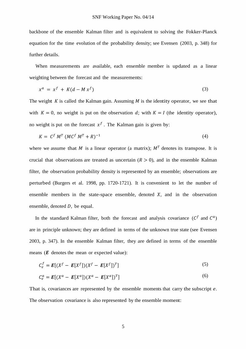
When measurements are available, each ensemble member is updated as a linear
weighting between the forecast and the measurements:
( ) (3)
The weight is called the Kalman gain. Assuming is the identity operator, we see that
with , no weight is put on the observation ; with (the identity operator),
no weight is put on the forecast . The Kalman gain is given by:
( ) (4)
where we assume that is a linear operator (a matrix); denotes its transpose. It is
crucial that observations are treated as uncertain ( ), and in the ensemble Kalman
filter, the observation probability density is represented by an ensemble; observations are
perturbed (Burgers et al. 1998, pp. 1720-1721). It is convenient to let the number of
ensemble members in the state-space ensemble, denoted , and in the observation
ensemble, denoted , be equal.
In the standard Kalman filter, both the forecast and analysis covariance ( and )
are in principle unknown; they are defined in terms of the unknown true state (see Evensen
2003, p. 347). In the ensemble Kalman filter, they are defined in terms of the ensemble
means ( denotes the mean or expected value):
[( [ ])( [ ]) ]
[( [ ])( [ ]) ]
(5)
(6)
That is, covariances are represented by the ensemble moments that carry the subscript .
The observation covariance is also represented by the ensemble moment:
SNF Working Paper No. 04/14
6
[( )( ) ] (7)
The observation ensemble is defined such that it has the true (given) observation as its
mean: [ ] . The ensemble Kalman gain is defined as
(
)
(8)
We assume that the ensemble is of sufficient size, such that and are
nonsingular; see Evensen (2003, p. 349). The analysis step (3) for ensemble member is
given by:
( ) ( ) ( ( ) ( )) (9)
It can be shown that by updating the ensemble with the perturbed observations , the
updated ensemble has the correct error statistics (Evensen 2003, p. 349). The analysis
covariance can be written as
( )
(10)
which is equivalent to the standard Kalman filter expression for the covariance matrix.
Please see Evensen (2003) for derivations and further discussion.
The filter can estimate parameters by adding the parameters to the state vector; in
essence by adding dimensions to the state-space. Parameters are treated as
unobserved, constant model states, which implies they are assumed to have zero drift
and diffusion terms (Hansen and Penland 2007, Kivman 2003). With parameters in
the state space, involved operators must adapt to make them compatible with the
extended state vector. The distribution of the ensemble members in the relevant
dimension of the state-space represents the conditional probability density function of
the parameter. We interpret the mean of the ensemble as the estimate and the spreading
of the ensemble as a measure of the estimate uncertainty.
The ensemble Kalman filter estimates state variables and parameters simultaneously.
As Evensen (2009, pp. 95-97) points out, the approach represents an improvement to
SNF Working Paper No. 04/14
7
more traditional approaches which ignore model error. The sequential nature of the
approach yields, for each observation time , parameter estimates conditional upon
observations up until ; estimates for the last observation are conditional upon all
observations and are usually the estimates of interest. In situations where regime shifts or
similar situations occur, one should inspect the behavior of the sequential parameter
estimates.
While the filter does not directly estimate the scaling of the diffusion term in (1),
the estimated can be used to infer the appropriate noise scaling.
estimates the
second moment of the density of the state vector at a given moment in time (at, say, ).
will vary with time (it is dynamic or flow- dependent; dynamic covariance is an advantage
with the ensemble Kalman filter over variational methods). The second moment of the
state vector density can be interpreted as the uncertainty in the estimated state
conditional upon the state at and the uncertain observation at . The uncertainty in
the state estimate accounts for parameter uncertainty, observational uncertainty, and
model inadequacy, the latter is what the diffusion term in (1) represents. Thus, if the
covariance is stable over time, or if it is stable after controlling for some assumed functional
form of the scaling term, like ( ) , can be interpreted as an estimate of
(or ). How varies over time maps out the distribution of , that is, we essentially
follow Hansen and Penland (2007).
The initial ensemble should reflect belief about the initial state of the system (Evensen
2003, p. 350). The filter can be initialized by specifying means and standard deviations
that characterize the initial ensemble. In the case of unknown parameters, initialization is
not necessarily straightforward. Our experience is that with large enough standard
deviations, such that the initial ensemble cover all eventualities, and enough ensemble
SNF Working Paper No. 04/14
8
members, it is possible to find reasonable traits of the initial ensemble. Often, there is
theory and earlier results to rely on.
For a given time , the ensemble Kalman filter provides an estimate of the state of the
system and its parameters conditional upon observations up until . By smoothing the
filter estimates, we obtain estimates conditional upon all observations (Evensen and van
Leeuwen 2000). The filter and smoother estimates for the final observation are identical,
and the smoothed parameter estimates are constant through time. The ensemble Kalman
smoother can be formulated as a sequential method and in terms of the filter analysis;
see Evensen (2003, p.360) for details. That smoother parameter estimates are constant
identical to the final filter estimate follows from the explicit modeling of parameters as
deterministic but unknown constants (see Hansen and Penland 2007 and Kivman
2003) and is straightforward from the formulation in terms of the filter estimates; see
Evensen (2009) for details. The ensemble Kalman smoother is particularly useful in
problems involving unknown parameters, as it provides estimates of the state variables
conditional upon observations and upon parameter estimates conditional upon all
observations. In contrast, the filter provides, for a given , state estimates conditional
upon observations up until and upon parameter estimates conditional upon
observations up until , which clearly are poor before the parameter estimate
converges.
To summarize, the ensemble Kalman filter can be interpreted as a statistical Monte
Carlo method where the ensemble evolves in state-space with the mean as the best
estimate and the spreading of the ensemble as the error variance (Burgers et al. 1998, p.
1720). For many problems, the sequential processing of observations proves to be a
better approach than the simultaneous processing which is typical in variational
methods (Evensen 2009, p. 101).
SNF Working Paper No. 04/14
9
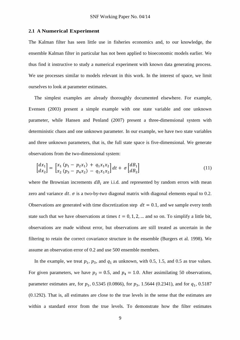
2.1 A Numerical Experiment
The Kalman filter has seen little use in fisheries economics and, to our knowledge, the
ensemble Kalman filter in particular has not been applied to bioeconomic models earlier. We
thus find it instructive to study a numerical experiment with known data generating process.
We use processes similar to models relevant in this work. In the interest of space, we limit
ourselves to look at parameter estimates.
The simplest examples are already thoroughly documented elsewhere. For example,
Evensen (2003) present a simple example with one state variable and one unknown
parameter, while Hansen and Penland (2007) present a three-dimensional system with
deterministic chaos and one unknown parameter. In our example, we have two state variables
and three unknown parameters, that is, the full state space is five-dimensional. We generate
observations from the two-dimensional system:
[
] [ ( ) ( )
] [
] (11)
where the Brownian increments are i.i.d. and represented by random errors with mean
zero and variance . is a two-by-two diagonal matrix with diagonal elements equal to 0.2.
Observations are generated with time discretization step , and we sample every tenth
state such that we have observations at times and so on. To simplify a little bit,
observations are made without error, but observations are still treated as uncertain in the
filtering to retain the correct covariance structure in the ensemble (Burgers et al. 1998). We
assume an observation error of 0.2 and use 500 ensemble members.
In the example, we treat , , and as unknown, with 0.5, 1.5, and 0.5 as true values.
For given parameters, we have , and . After assimilating 50 observations,
parameter estimates are, for , 0.5345 (0.0866), for , 1.5644 (0.2341), and for , 0.5187
(0.1292). That is, all estimates are close to the true levels in the sense that the estimates are
within a standard error from the true levels. To demonstrate how the filter estimates
SNF Working Paper No. 04/14
10
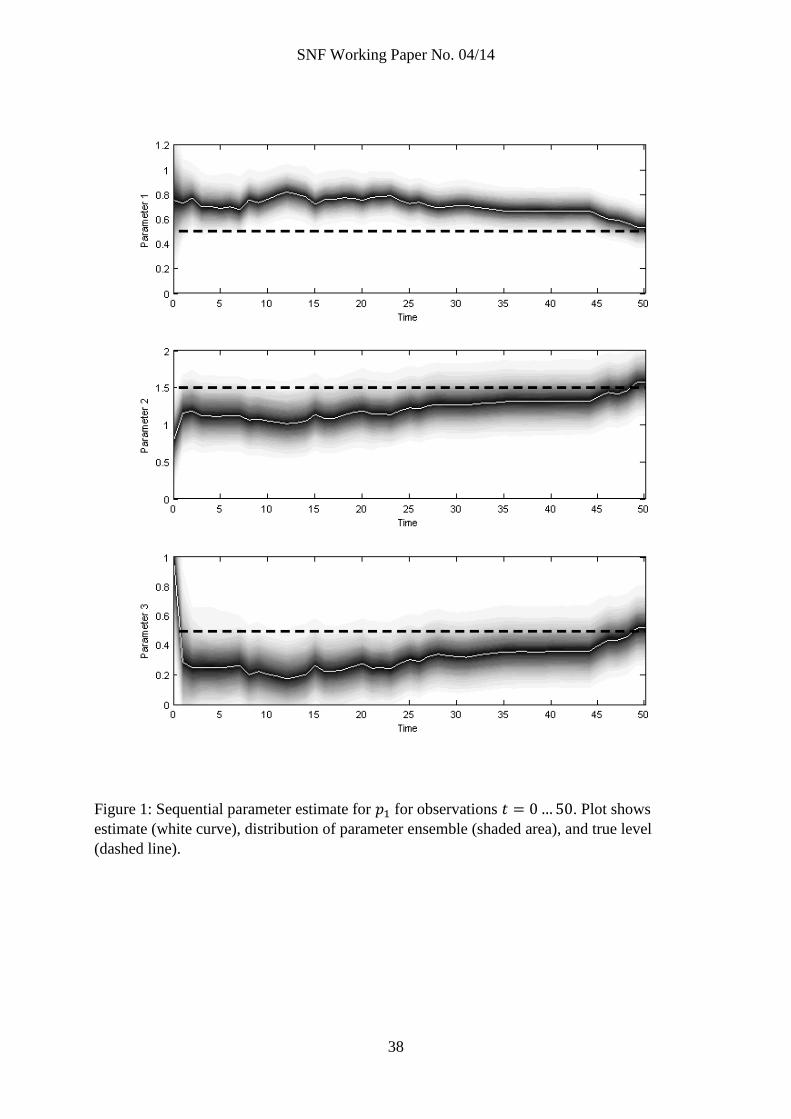
parameters in a sequential fashion, figure 1 displays the parameter estimates (white curve), the
distributions of the parameter ensembles (shaded areas; darker shade means higher density of
ensemble particles), and for comparison, the true parameter levels (dashed line). The top
panel shows ; the middle panel shows ; and the bottom panel shows . From the figure,
we see that while the ensemble contracts considerably with the first few observations, it takes
many more observations for the estimates to converge on the true levels.
3 The Barents Sea Model
The Barents Sea is one of the most productive ocean areas in the world, and is subject to
extensive research (Gjøsæter et al. 2009, Huse et al. 2004, Durant et al. 2008, see also
further references therein). The commercially most important stocks are cod (Gadus
morhua) and capelin (Maooltus villosus); cod is highly valued as human food and capelin is
an important part of the cod diet. Capelin is also caught for fishmeal and oil production.
Juvenile herring (Clupea harengus L.) enters the Barents Sea when large year-classes arise
in the Norwegian Sea. Herring has an important influence on the ecosystem; it is preyed
on by cod while it preys on capelin larvae. We limit our model to these three fish stocks
for two main reasons. First, our model captures the dynamics of the cod stock to a high
degree, and the cod fishery is the most important fishery in the region and of our main
interest. Second, if the model is to be relevant for bioeconomic analysis, we have to limit
the complexity and dimensionality of the model. We have in mind the type of analysis
carried out in Sandal and Steinshamn (2010) and Poudel et al. (2012); see also Kugarajh
et al. (2006).
To limit complexity, we use simple growth functions and interaction terms common
in traditional bioeconomic analysis. While dimensionality is based upon technical
limitations, we find comfort in the view promoted by Holling and Meffe (1996, p.
SNF Working Paper No. 04/14
11
333), that the driving forces of an ecosystem are confined to a relatively small subset of
variables and relationships. While our choice of variables and relationships does not
contain all driving forces of the Barents Sea ecosystem, we observe that our model
captures much of the variation detected in stock assessments.
3.1 The Main Model
The biomass of the three stocks are the state variables; cod is denoted , capelin is
denoted , and herring is denoted . Both cod and capelin are harvested in the Barents
Sea; and denote harvest rates of cod and capelin. Herring is not harvested in the
Barents Sea, but eggs and larvae flow in from the Norwegian Sea. We denote the inflow by
. Finally, we denote parameters and vectors in boldface. The dynamic model for the
system is written, on differential form:
( ( ) ( ) ( ) ) ( )
( ( ) ( ) ( ) ) ( )
( ( ) ( ) ( ) ) ( )
(12)
(13)
(14)
where growth functions are denoted ; interaction terms are denoted . Table 1 report
functional forms that we discuss further below. The stochastic increments are
independent, with mean zero and variance . The scaling term ( ) reflect correlations
in the noise processes. Two principal models of the scaling term were tried; white noise
( ( ) ) and, inspired by the stochastic term in the geometric Brownian motion,
state-dependent white noise ( ( ) ) .
The first terms in each model equation are the growth functions. The growth functions
model the growth that does not happen through the modelled interactions. For cod
(equation 12), we use the logistic growth function; for the pelagic stocks capelin (equation
13) and herring (equation 14), we use the modified logistic growth function (see Table 1
SNF Working Paper No. 04/14
12
for specifications). The related parameters ( , , , , , and ) are interpreted
accordingly. (The idea of carrying capacity; the standard interpretation of the second
parameter in the logistic and modified logistic, becomes unclear in an ecosystem
setting. The capacity of the ecosystem to harbor any one specie depends on the state of
the entire system. Hence, intrinsic, single species notions such as carrying capacity must
be treated with caution in our multispecies approach.)
All species interactions in the system are predator-prey relationships. Cod preys
upon both herring and capelin, while herring preys upon the capelin stock. (A
competitive, mutually destructive interaction between the pelagic species is an
alternative that we discuss briefly below.) The interaction terms are per definition
positive, and the mirror terms (cod-capelin mirrors capelin-cod, for example) have
opposite signs. The capelin-cod and capelin-herring interaction terms ( ( )) are
inspired by the crude form of predator-prey interaction (May et al. 1979, p. 268),
where the product of the stock levels are adjusted by an intensity parameter. The
functional form of, for example, the capelin-cod interaction is ( ) ,
where is the intensity parameter. We will discuss the interpretation of the
interaction intensity parameter further below.
The cod-herring interaction model is based on the Lotka-Volterra model, but
modified to allow cod to prefer capelin (Durant et al. 2008, Gjøsæter et al. 2009). We
have the interaction term ( )
. is the interaction intensity
parameter. The fraction term yields a model of preference. Without capelin present
( ), the Lotka-Volterra term remains undisturbed (the fraction equals one).
When capelin is present, the fraction takes a value between zero and one and weakens
the interaction.

SNF Working Paper No. 04/14
13
As is evident from the model equations (12 - 14), the interaction terms and
represent a biomass loss for the prey species and a biomass gain for the predator
species. The intensity parameters scale the product of biomasses in the terms to
account for the rate of biomass loss in the prey species. Biomass is not conserved in the
interactions, and the additional interaction parameters ( , , and ) account for the
loss of biomass in the interactions. The additional interaction parameters take values
between zero and one, and since most of the biomass is lost, they are expected to lie
closer to zero than one. We think of the additional interaction parameters as biomass
conversion rates between species. Presumably, regularities exist for biomass conversion
rates. While known or assumed interaction relationships would be helpful in reducing the
number of parameters in the model, biologists are skeptical when it comes to the
stability of the relationships (S. Tjelmeland, personal communication). Thus, we refrain
from prescribing fixed relationships.
The final parameter measures the influence of the inflow of herring on the herring
stock growth. Most of the time, the amount of herring biomass which enters the Barents
Sea is relatively small. After a few years, however, the herring has grown substantially.
Thus, we lag the inflow variable two years and multiply it with the scaling parameter .
The idea is that three year old (and older) herring makes out most of the herring biomass
in the Barents Sea, and the biomass influx two years earlier better explains the change in
the herring stock. (After three or four years in the Barents Sea, the juvenile herring
returns to its main habitat in the Norwegian Sea to mature and eventually spawn; the
herring growth rate in our model reflect the migration behavior.)
To avoid negative parameters, parameters are all assumed to be log-normal distributed.
(Theoretically, they are treated as ( ), where each is a stochastic constant
which is normal distributed.)
SNF Working Paper No. 04/14
14
We treat estimates from stock assessments as measurements of the state variables,
and the measurement operator is thus the identity operator. Note that parameters are
added to the state vector as described above. We denote the extended state vector .
The measurement operator must thus be adjusted to be compatible with the state
vector by adding zeros. Parameters are treated as unobserved states. The observation
equation becomes
(15)
where
[
], [ ], [ ], and [ ]
(16)
is a three by three identity matrix and is a three by thirteen zero matrix. is a
three-element vector of observations, and is the error term vector which is normal,
independent, and identically distributed with mean zero and variance .
3.2 The Alternative Model
While we keep our main focus on the model above, we also study an alternative model
with fewer parameters. In the alternative model, the pelagic species capelin and herring
have a common carrying capacity. A common carrying capacity is equivalent to a
competitive, mutually destructive interaction, but has fewer parameters. Ekerhovd and
Kvamsdal (2013) successfully pursue the common carrying capacity idea in a model of the
pelagic species in the Norwegian Sea. We write the model as follows
( ( ) ( ) ( ) ) ( )
( ( ) ( ) ) ( )
( ( ) ( ) ) ( )
(17)
(18)
(19)
The new parameter is the common carrying capacity in the growth function
( ) (see table 1). replaces and in the main model. As the capelin-
SNF Working Paper No. 04/14
15
herring interaction is incorporated into the growth function, the interaction term
( ) (and the related ) has become superfluous. The system is otherwise
identical to the main model above. In an attempt to avoid confusion, parameter numbers
are kept from the main model when parameters have the same role and interpretation in
the model. Thus, the parameter vector in the alternative model is
[ ] . The observation equation (15) is the same as
before, but in [ ], is a three by ten zero matrix to conform to the dimensionality
of the extended state vector, which is
[
], [ ], [ ]
(20)
3.3 Data
The fish stocks in the Barents Sea cannot be observed directly. However, the Institute of
Marine Research in Bergen and the Knipovich Polar Research Institute of Marine
Fisheries and Oceanography in Murmansk carry out extensive, yearly ecosystem surveys.
Based upon these surveys, they provide yearly estimates of the stock levels of all the
important species in the Barents Sea. The stock estimates are published by the
International Council for the Exploration of the Sea (ICES), and most of our data are
collected from the ICES online database. We treat the stock estimates as observations.
Notably, Ekerhovd and Gordon (2013) raises issues with stock estimates from virtual
population models. We share their concern about the consistency in the stock estimates,
but find it beyond our scope to apply the (Ekerhovd and Gordon 2013) adjustment here.
Uncertainty in stock assessments are unfortunately not reported, and we are left to
speculate. The herring inflow data was provided by S. Tjelmeland (personal
communication).
SNF Working Paper No. 04/14
16
We have stock estimates, catch data and herring inflow estimates from 1950 to
2007. However, the ICES database does not contain data on capelin prior to 1972. For
the period prior to 1972, we collected catch data from Røttingen and Tjelmeland (2008,
see Figure 2). Capelin stock estimates were collected from Marshall et al. (2000, see
Figure 1, p. 2435). The early capelin stock estimates are more uncertain than later
estimates, and we assume a 50% increased observation uncertainty on the capelin
stock data prior to 1972.
All data are visually presented in Figure 2, with error bars showing assumed
observation uncertainty. All numbers are measured in tonnes.
3.4 Estimation Strategy and the Initial Ensemble
While the success of our approach hinges to some degree on reasonable characteristics of
the initial ensemble, what constitute reasonable characteristics is not immediately clear.
While for a few of the parameters in the interaction terms, we can rely on external,
empirical evidence, we must produce reasonable initial ensemble characteristics for most
parameters in a heuristic fashion. The parameter subspace has thirteen dimensions in the
main model (one for each parameter), and while it is not impossible to search, via trial
and error, the parameter subspace for an appropriate, initial ensemble, the high
dimensionality makes the approach unlikely to succeed. (Our main metrics of
appropriateness are whether the state estimates resemble the stock assessment data and to
what degree the spread of the ensemble in the parameter dimensions contracts over time.
In addition, we have used the Bayesian Information Criterion (BIC), but carefully, since
the criterion is not unique because of the Monte Carlo element of the filter (see Ekerhovd
and Kvamsdal 2013, pp. 8-9). Finally, we have also considered the distribution of the
Kalman gain over time; gain terms close to one suggest a poor initial ensemble.)
SNF Working Paper No. 04/14
17
By first assimilating each equation individually, we reduce the dimensionality of the
relevant parameter subspace substantially. When we assimilate the cod equation (12), for
example, the state space consist of the cod stock level as the only state variable and the four
parameters in the equation ( - ) as parameter variables. The variables and are
treated as control variables.
We have good ideas about reasonable ensemble initializations of the biomass
conversion rates (limited support) and the interaction intensity parameters for the cod-
capelin and cod-herring interaction terms (empirical evidence). The capelin-herring
interaction intensity is assumed to be an order smaller than the cod-capelin interaction
intensity. Thus, when searching for reasonable initial ensemble characteristics in the
single equation assimilations, we need mostly to be concerned with the parameters of the
growth functions. What we have called the capacity parameters are characterized by an
ensemble mean higher than observed historic levels (exploited fisheries usually have stock
levels below their full capacity). To find reasonable characteristics for the ensembles
along the growth rate dimensions, we consider a range of levels and compare, as
mentioned above, model fit, ensemble contraction, the Bayesian Information Criterion,
and the distribution of the Kalman gain. To demonstrate, we briefly discuss an example
of the procedure in appendix A.2. Means and spreads of the initial ensemble for the
parameter dimensions in the single equation assimilations are listed in Table A2 in the
appendix.
The estimates from the single equation assimilations are used to characterize the mean
of the normal distributions from which we draw the initial ensemble for assimilation of the
full model. Exceptions are those parameters for which we have empirical support for the
initial ensemble characteristics. Ensemble spreads (standard deviations of distributions
SNF Working Paper No. 04/14
18
from which initial ensembles are drawn) are also inherited from the single equation
assimilations, with the same exceptions.
The initial ensemble is drawn randomly from a multivariate normal distribution. For
the three state variables, we use the first observations as the mean of the initial
ensemble and 30% of the first observation as standard deviation.
The initial ensemble for the interaction intensity parameters , , and were
characterized based upon empirical evidence. The term ( ) in (13)
reflects the loss of capelin biomass from the interaction with cod. Gjøsæter et al.
(2009, see Figure 5, p. 45) estimated, from stomach content data, the amount of
capelin consumed by the Barents Sea cod for the years 1984-2006. The consumption
varies over time, as does the cod and capelin stock levels. To get a reasonable initial
measure of , we regressed the total consumption of capelin on the product
(without intercept). Notably, Gjøsæter et al. (2009) provided us with data for 1984-
2007 (that is, one more year of data than what they based their original analysis upon).
The estimated coefficient was (standard error , ).
Similar data for the capelin-herring interaction are not available. Herring is however
thought to have a smaller predation rate on capelin than cod; we set the implied mean
for at 10% of the implied mean of . For the herring-cod interaction intensity
parameter , data are available. As for capelin, Gjøsæter et al. (2009) estimated the
amount of herring consumed by the Barents Sea cod. Regressing the consumed
amount of herring on the term
yielded a coefficient of
(standard error , ). As with , we set the mean of the initial
shadow parameter ( ) ensemble to correspond to the estimated coefficient. In
comparison, regressing on the term produces the coefficient
(standard error , ).
SNF Working Paper No. 04/14
19
The additional interaction parameters , , and (biomass conversion rates)
cannot be larger than one as it is assumed that some biomass is lost in the interactions.
The biomass loss assumption is not explicitly enforced, but initial implied ensemble means
for the three additional interaction parameters were set to 0.25 for and 0.1 for and
. Typically, one assumes that 90% of the biomass is lost between trophic levels, but cod
spends less energy catching capelin and thus we specified a higher additional interaction
parameter for the cod-capelin interaction.
We discuss further implementation details in appendix A.1.
4 Results
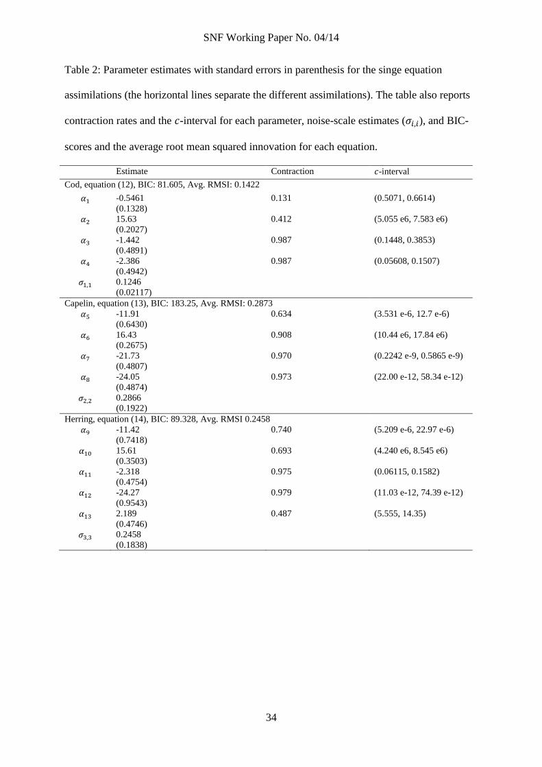
Table 2 reports parameter estimates, with standard errors in parenthesis, for the single
equation assimilations. Table A2 in the appendix reports the prior characterizations for
comparison. The third column (‘Contraction’) in table 2 reports the standard error of the
estimates as a fraction of the standard deviation of the prior distribution. The ensemble
Kalman filter will mechanically contract parameter ensembles, but the amount of
contraction depends on the amount of information the filter retains. Assessing the
contraction is equivalent to compare the width of the parameter confidence intervals at
the beginning and end of the assimilation. Both tables and also subsequent tables report
estimates of the shadow parameters . But our interest lies with the parameters
( ), and table 2 report what we call the -interval, which is the two standard
error interval around the mean estimate of the underlying parameter .
As in the numerical examples, we also calculate an estimate and standard error of
the parameters in the diffusion terms. We denote the parameters , where the subscript
denote the relevant state variable. Table 2 reports the results.

SNF Working Paper No. 04/14
20
Further, table 2 reports the BIC-scores and the average root mean squared
innovations for each equation. The BIC-scores, both here and later, are evaluated with a
data neighborhood radius of 200.000 (tonnes); see Ekerhovd and Kvamsdal (2013) for
details. The neighborhood radius is comparable to the bandwidth concept in kernel-type
approaches. The innovation is the distance between the observations and the
estimated state variables. In our model, with the state-dependent noise scaling , it
is useful to normalize the root mean squared innovations with the estimated state. So,
what we report as the average root mean squared innovation is the time-average of the
following expression
√ [( ) ]
[ ]
(21)
The subscript is just a reminder that it is the smoothed estimate that goes into the
expression. The lower the average root mean squared innovation, the better is the model
fit. Note that in absence of the normalization issue, the average root mean squared
innovation is the average distance between the ensemble members and the observation; if
the observation and the ensemble mean are close, the average root mean squared
innovation will be close to the estimate of the noise scaling term, which is derived from the
second moment of the ensemble.
To discuss the actual estimates in table 2 is of limited interest; their main function is
to serve as priors for the full model. We do note, however, that while the contraction
rate is significant for most other parameters, the interaction parameters (parameters
3,4,7,8,11, and 12) have not contracted much. As the full model results will show,
contraction is somewhat better when we assimilate all equations simultaneously. The
small contraction rates for the interaction parameters underlines the need for
informative priors.
SNF Working Paper No. 04/14
21
The cod equation has both the smallest BIC-score and average root mean squared
innovation. Also, the noise scaling parameter is clearly statistical significant for the cod
cod equation, while less clearly so for the other equations. We conclude that of the three
equations, the cod equation serves its purpose best.
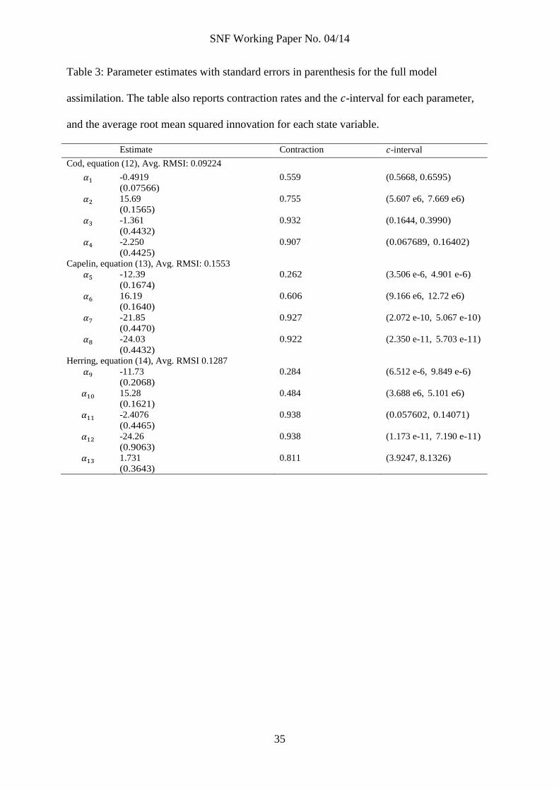
Table 3 reports results for the full model assimilation. The BIC-score for the entire
model is 265.94. Notably, the prior for the full model assimilation is based upon the results
reported in table 2 for all parameters apart from the two parameters for which we have
empirical evidence ( and ). For those parameters, we kept the original prior
information as given in table A2.
If we compare the contraction rates reported in tables 2 and 3, we observe that overall,
contraction is better in the full model assimilation for the capelin and herring equation. In
the cod equation, the interaction parameters have better contraction rates in the full
model assimilation, while the growth parameters contracts better in the single equation
assimilation. That the growth parameters does not contract as much in the full model
assimilation is likely because most of the signal in the data about these parameters is
picked up in the single equation assimilation that was run prior to the full model
assimilation.
Upon further comparison of the results in tables 2 and 3, we note that many
parameters are significantly improved in the full model assimilation (in the latter table,
estimates are several standard errors away from their prior in the former table). We also
note that the average root mean squared innovations have improved considerably for all
state variables. As discussed above, the average root mean squared innovations can be
close to the estimate if the ensemble mean is close to the observations. Further,
significant cross-correlations in (the off-diagonal terms) may be challenging in model
applications; as we report below, estimated cross-correlations are close to zero.
SNF Working Paper No. 04/14
22
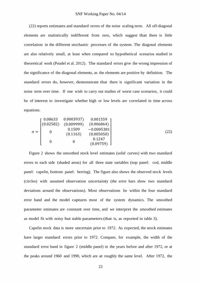
(22) reports estimates and standard errors of the noise scaling term. All off-diagonal
elements are statistically indifferent from zero, which suggest that there is little
correlation in the different stochastic processes of the system. The diagonal elements
are also relatively small, at least when compared to hypothetical scenarios studied in
theoretical work (Poudel et al. 2012). The standard errors give the wrong impression of
the significance of the diagonal elements, as the elements are positive by definition. The
standard errors do, however, demonstrate that there is significant variation in the
noise term over time. If one wish to carry out studies of worst case scenarios, it could
be of interest to investigate whether high or low levels are correlated in time across
equations.
[ ( )
)( )
( )
( )
( )
( ) ]
(22)
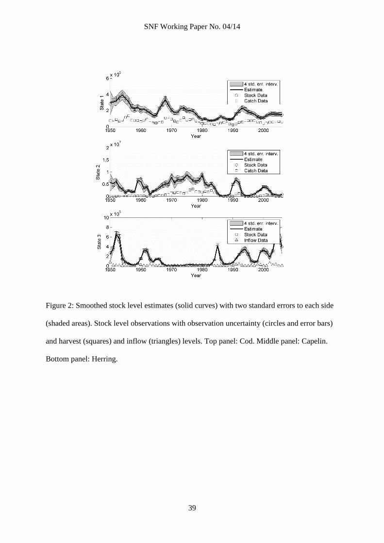
Figure 2 shows the smoothed stock level estimates (solid curves) with two standard
errors to each side (shaded areas) for all three state variables (top panel: cod, middle
panel: capelin, bottom panel: herring). The figure also shows the observed stock levels
(circles) with assumed observation uncertainty (the error bars show two standard
deviations around the observations). Most observations lie within the four standard
error band and the model captures most of the system dynamics. The smoothed
parameter estimates are constant over time, and we interpret the smoothed estimates
as model fit with noisy but stable parameters (that is, as reported in table 3).
Capelin stock data is more uncertain prior to 1972. As expected, the stock estimates
have larger standard errors prior to 1972. Compare, for example, the width of the
standard error band in figure 2 (middle panel) in the years before and after 1972, or at
the peaks around 1960 and 1990, which are at roughly the same level. After 1972, the
SNF Working Paper No. 04/14
23
capelin stock estimates, in addition to being more precise, lie closer to the measurements.
4.1 Alternative Model Results
In the alternative model, the initial ensemble for to is characterized by the prior
estimates in table 2. If we assimilated equations (18) and (19) individually, we would get
two different prior estimates for . Using some kind of average of the two priors could
work in practice, but theoretically the initial ensemble would be suboptimal for both the
capelin and herring equation. Agreeing priors would bode well for the approach, and
could be taken as a sign of a well-posed model. In our alternative model, priors from
assimilating the capelin and herring equations individually did not agree to a satisfying
degree, and the resulting initial ensemble for the full model was not ideal.
Rather than assimilate equations (18) and (19) individually, we assimilated them
together as a system with two state variables and six parameters. was treated as a
control variable as in the single equation assimilations in the main model. Table 4 reports
results from assimilating the capelin-herring system. As prior for the new parameter ,
we used the higher of the two parameters replaced (it replaced and in the main
model).
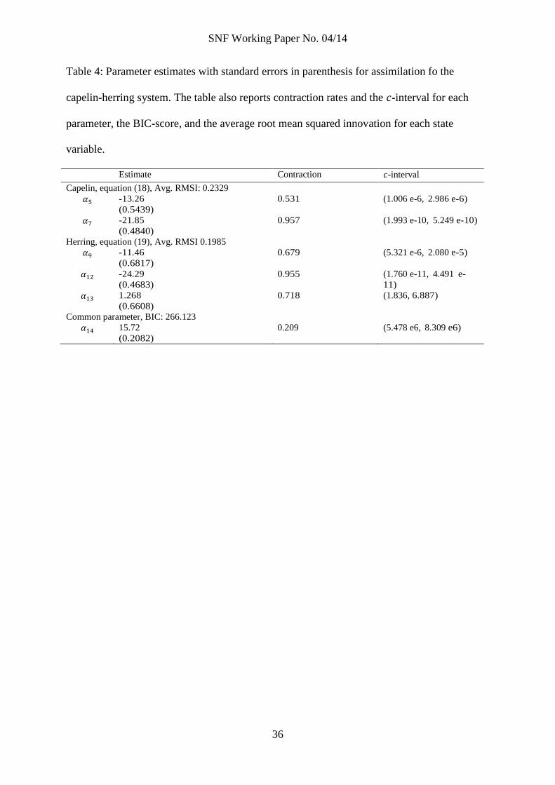
Contraction of the parameter ensemble is significant in the capelin-herring assimi-
lation, and, for most parameters, better than corresponding contraction rates in the single
equation assimilation of the main model. In fact, the contraction in the ensemble was
so strong that the full model suffered from divergence with the narrow ensemble. To avoid
introducing ad-hoc measures such as inflation (Anderson and Anderson 1999), we increased
the standard deviation of the prior to 1 in the full model. As in the main model, the
interaction parameters ( and ) did not contract much and there is a clear need for
informative priors.

SNF Working Paper No. 04/14
24
(23) reports estimates and standard errors of the noise-scaling term in the capelin-
herring system. The estimates are higher than the corresponding estimates in (22), but
smaller than the estimates in the single equation assimilations of the main model (table
2). As in (22), the off-diagonal term is statistically indifferent from zero.
[
( )
( )
( )
] (23)
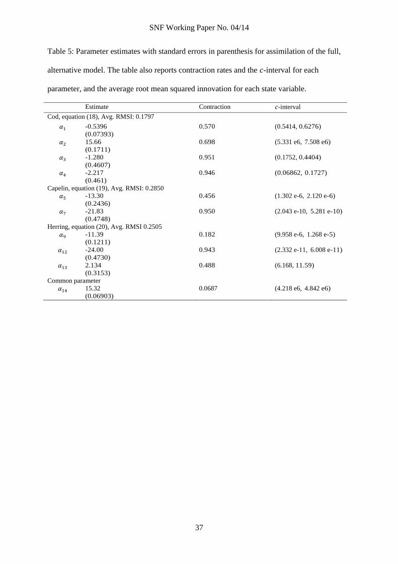
Table 5 reports results from assimilating the full, alternative model. Contraction
rates are better than in the prior assimilation (table 4) for most parameters and follows
essentially the same pattern as in the main model. The BIC-score for the full,
alternative model is 465.23; significantly higher than the BIC-score of the main model
despite the preference of the BIC-statistic for models with fewer parameters.
If we compare the results in table 5 to the results for the main model in table
3, it is first of all clear that parameters of the cod equation are not statistically different.
The interaction parameters ( and ) are also not statistical different in the two
models. The inflow scaling parameter is more different in the two models, but the
estimates are still only slightly more than a standard error away from each other, and
statistical tests cannot distinguish between them.
The remaining parameters in table 5, growth rates , and the common carrying
capacity are, however, quite different than the comparable parameters in the main
model. While the capelin growth rate is much lower, the herring growth rate is higher.
The common carrying capacity is much lower than the capelin capacity parameter in the
main model ( ), but within the range of the herring capacity ( ). While the expected
change in the herring growth rate is unclear when the common capacity is within the
range of the capacity in the main model, the expected change in the capelin growth rate
would be a higher rate when the common capacity in the alternative model is lower
SNF Working Paper No. 04/14
25
than in the main model. We are puzzled about this behavior of the alternative model, not
the least because from a phenomenological perspective, the estimated alternative model is
unacceptable with the carrying capacity well below observed historical levels of the
exploited fishery. But, the higher average root mean squared innovations in the alternative
model than in the main model suggest the general model fit is better in the main model,
and with the better BIC-score of the main model we conclude that the main model is the
most appropriate model.
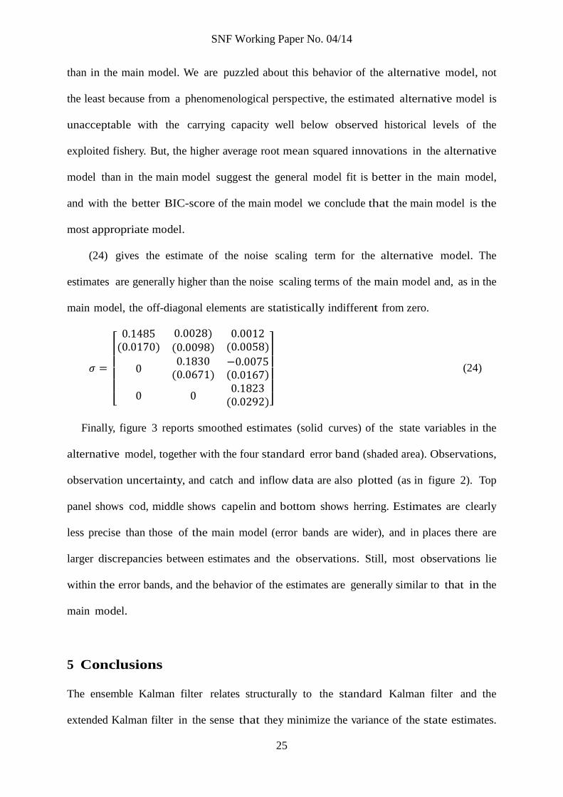
(24) gives the estimate of the noise scaling term for the alternative model. The
estimates are generally higher than the noise scaling terms of the main model and, as in the
main model, the off-diagonal elements are statistically indifferent from zero.
[ ( )
)( )
( )
( )
( )
( )]
(24)
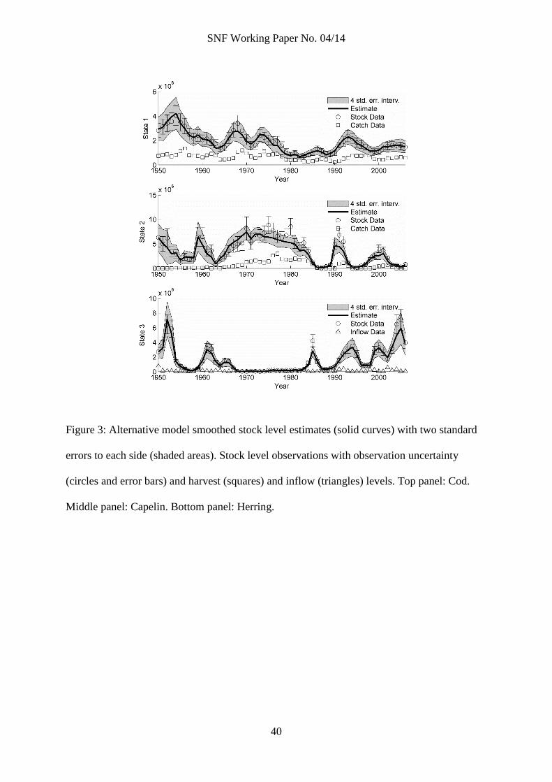
Finally, figure 3 reports smoothed estimates (solid curves) of the state variables in the
alternative model, together with the four standard error band (shaded area). Observations,
observation uncertainty, and catch and inflow data are also plotted (as in figure 2). Top
panel shows cod, middle shows capelin and bottom shows herring. Estimates are clearly
less precise than those of the main model (error bands are wider), and in places there are
larger discrepancies between estimates and the observations. Still, most observations lie
within the error bands, and the behavior of the estimates are generally similar to that in the
main model.
5 Conclusions
The ensemble Kalman filter relates structurally to the standard Kalman filter and the
extended Kalman filter in the sense that they minimize the variance of the state estimates.
SNF Working Paper No. 04/14
26
However, the ensemble Kalman filter has some advantages. Unlike the extended Kalman
filter, it requires no linearization. It solves rank problems that may occur with large
numbers of observed variables. Unlike variational adjoint methods, it requires no adjoint
operator and is thereby simpler to implement, and it has flow-dependent (non-constant)
covariance. Further, the ensemble Kalman filter is well suited to large-scale problems and it
extends to asynchronous observations. On the other hand, the ensemble integration (in the
forecast step) can be computationally costly and, with strongly nonlinear systems,
iterative procedures called multiple data assimilations holds better promise (Emerick and
Reynolds 2012). As such, the ensemble Kalman filter is just the tip of the iceberg that
consist of a range of related methods that apply to a range of different problems (Evensen
2003).
In applying the ensemble Kalman filter, we have shown how relatively simple
aggregated biomass models, typical in bioeconomic analysis, can capture much of the
dynamics of ecosystems. When compared to earlier efforts of applying data assimilation
methods to bioeconomic models (Ussif et al. 2003), our results are superior. Our main
model shows the most promise; as discussed above, the alternative model has a number
of undesirable properties that, when added together, wipe out the advantage of fewer
parameters. Also other variations of the main model was assimilated; pure, white (not
level dependent) noise in the error term, assumed perfect observations of the control
variables (catch and inflow), model herring inflow as a state variable, and model herring
inflow as white noise around a non-zero mean. None of the variations lead to
significant improvements, if any, in model fit or parameter estimates.
A prominent modeling possibility that could be explored is data timing. In our current
approach, we assume a constant harvest rate through each year. The harvesting occurs
more concentrated in winter and spring, however. Further, the stock assessments are

SNF Working Paper No. 04/14
27
usually carried out in the fall. These nuances of timing could influence the dynamics of
the system were they taken into account. We have chosen not to go into this in our
current approach for two reasons. One is a need to limit the scope of our work. A second
and more important is that our current approach better serves the model needs in a
bioeconomic framework for decision and management analysis.
The main model does of course have room for other improvements. The -interval for
several of the parameters are not particularly tight, for example, and the estimates of
elements in the matrix are not very precise. Based upon our experience, we conclude
that the best source of improvements would be more data. While some of the series we
use here extend further than what we utilize, herring inflow estimates are not further
available. Notwithstanding, estimates of parameters in chaotic systems are not likely to
be very precise, and management models should be flexible and adaptive (Holling and
Meffe 1996, p. 332). It is important that management models take the uncertainty of the
dynamics into account (Hill et al. 2007). Adaptive management models such as feedback
models are already well understood in the bioeconomic literature (Sandal and Steinshamn
1997). The challenge is to solve models of higher dimensionality that must underlie
ecosystem-based management (Fulton et al. 2011). We believe the ensemble Kalman
filter has an important role to play in both theoretical and operational management
research, particularly in light of the recent calls for ecosystem-based management (Pew
Oceans Commission 2003).
In the broader scope of things, we aim to answer calls for ‘flexible, adaptive, and
experimental’ management models (Holling and Meffe 1996, p. 332), who further write
that ‘effective natural resource management that promotes long- term system viability
must be based on an understanding of the key processes that structure and drive
ecosystems, and on acceptance of both the natural ranges of ecosystems variation and the

SNF Working Paper No. 04/14
28
constrains of that variation for long-term success and sustainability’ (p. 335). We
think that, when models are simplified and reduced down to the key driving
phenomena, the ensemble Kalman filter can capture variabilities and stabilities of
ecosystems and serve tractable management models.
Acknowledgements
We are grateful to Geir Evensen, Laurent Bertino, Sigurd Tjelmeland, and Jonas
Andersson. We acknowledge financial support from the Norwegian Research Council,
project number 196433/S40.
References
Anderson, Jeffrey L., Stephen L. Anderson. 1999. A Monte Carlo implementation of the
nonlinear filtering problem to produce ensemble assimilations and forecasts.
Monthly Weather Review 127(12) 2741–2758.
Burgers, Gerrit, Peter Jan van Leeuwen, Geir Evensen. 1998. Analysis scheme in the
ensemble Kalman filter. Monthly Weather Review 126(6) 1719–1724.
Durant, J. M., D. Ø. Hjermann, P. S. Sabarros, N. C. Stenseth. 2008. Northeast Arctic
cod population persistence in the Lofoten-Barents Sea system under fishing.
Ecological Applications 18(3) 662–669.
Ekerhovd, N.-A., D. V. Gordon. 2013. Catch, stock elasticity and an implicit index of
fishing effort. Marine Resource Economics 28(4).
Ekerhovd, N.-A., S. F. Kvamsdal. 2013. Modeling the Norwegian Sea ‘Pelagic Complex.’
An application of the ensemble Kalman filter. Institute for Research in Economics
and Business Administration Working Paper 7.
SNF Working Paper No. 04/14
29
Emerick, A. A., A. C. Reynolds. 2012. History matching time-lapse seismic data using
the ensemble Kalman filter with multiple data assimilations. Computational
Geoscience 16 639–659.
Evensen, Geir. 2003. The Ensemble Kalman Filter: Theoretical formulation and practical
implementation. Ocean Dynamics 53 343–367.
Evensen, Geir. 2009. Data Assimilation: The ensemble Kalman filter. 2nd ed. Springer-
Verlag, Berlin Heidelberg.
Evensen, Geir, Peter Jan van Leeuwen. 2000. An ensemble Kalman smoother for nonlinear
dynamics. Monthly Weather Review 128(6) 1852–1867.
Fulton, E. A., J. S. Link, I. C. Kaplan, M. Savina-Rolland, P. Johnson, C. Ainsworth, P.
Horne, R. Gorton, R. J. Gamble, A. D. M. Smith, D. C. Smith. 2011. Lessons in
modelling and management of marine ecosystems: the Atlantis experience. Fish
and Fisheries 12(2) 171–188.
Gjøsæter, Harald, Bjarte Bogstad, Sigurd Tjelmeland. 2009. Ecosystem effects of the three
capelin stock collapses in the Barents Sea. Marine Biology Research 5 40–53.
Grønnevik, Rune, Geir Evensen. 2001. Application of ensemble-based techniques in fish
stock assessment. Sarsia 86 517–526.
Hannesson, Rognvaldur. 2007. Cheating about the Cod. Marine Policy 31 698–705.
Hansen, James A., Cecile Penland. 2007. On stochastic parameter estimation using data
assimilation. Physica D 230(1-2) 88–98.
Hill, S. L., G. M. Watters, A. E. Punt, M. K. McAllister, C. L. Quer e, J. Turner. 2007.
Model uncertainty in the ecosystem approach to fisheries. Fish and Fisheries 8(4)
315–336.
SNF Working Paper No. 04/14
30
Holland, Daniel S., James N. Sanchirico, Robert J. Johnston, Deepak Joglekar. 2010.
Economic Anlysis for Ecosystem-Based Managment: Applications to Marine and
Costal Environments . RFF Press, Washington. D.C
Holling, C. S., Gary K. Meffe. 1996. Command and control and the pathology of natural
resource management. Conservation Biology 10(2) 328–337.
Huse, Geir, Geir O. Johansen, Bjarte Bogstad, Harald Gjøsæter. 2004. Studying spatial
and thropic interactions between capelin and cod using individual- based
modelling. ICES Journal of Marine Science 61 1201–1213.
Kaufman, Les, Burr Heneman, J. Thomas Barnes, Rod Fujita. 2004. Transition from low
to high data richness: An experiment in ecosystem-based fishery management
from California. Bulletin of Marine Science 74(3) 693–708.
Kivman, G. A. 2003. Sequential parameter estimation for stochastic systems. Nonlinear
Processes in Geophysics 10 253–259
Kugarajh, Kanaganayagam, Leif K. Sandal, Gerhard Berge. 2006. Implementing a
stochastic bioeconomic model for the North-East Artic cod fishery. Journal of
Bioeconomics 8(1) 35–53.
Ludwig, Donald, Ray Hilborn, Carl Walters. 1993. Uncertainty, resource exploitation, and
conservation: Lessons from history. Science 260(5104) 17, 36.
Marshall, C. Tara, Nathalia A. Yaragina, Bjørn Adlandsvik, Andrey V. Dolgov. 2000.
Reconstructing the stock-recruit relationship for Northeast Artic cod using a
bioenergetic index of reproductive potential. Canadian Journal of Fisheries and
Aquatic Sciences 57(12) 2433–2442.
May, Robert M., John R. Beddington, Colin W. Clark, Sidney J. Holt, Richard M.
Laws. 1979. Management of multispecies fisheries. Science 205 267–277.
SNF Working Paper No. 04/14
31
Pew Oceans Commission. 2003. America’s living oceans-charting a course for sea change.
recommendations for a new ocean policy. Tech. rep., Pew Foundation,
Washington, D.C.
Poudel, D., L. K. Sandal, S. I. Steinshamn, S. F. Kvamsdal. 2012. Do species interaction
and stochasticity matter to optimal management of multispecies fisheries? G. H.
Kruse, H. I. Browman, K. L. Cochrane, D. Evans, G. S. Jamieson, P. A. Livingston,
D. Woodby, C. I. Zhang, eds., Global Progress in Ecosystem-Based Fisheries
Management . Alaska Sea Grant, University of Alaska Fairbanks, 209–236.
Røttingen, Ingolf, Sigurd Tjelmeland. 2008. A quest for management objectives - case
study on the Barents Sea Capelin. ICES 2008 Annual Science Conference, Halifax,
Nova Scotia, Canada . O:08, ICES CM Documents 2008.
Sandal, Leif K., Stein I. Steinshamn. 1997. A stochastic feedback model for optimal
management of renewable resources. Natural Resource Modeling 10(1) 31–52.
Sandal, Leif K., Stein I. Steinshamn. 2010. Rescuing the prey by harvesting the
predator: Is it possible? Endre Bjørndal, Mette Bjørndal, Panos M. Pardalos,
Mikael Ronnqvist, eds., Energy, Natural Resources and Environmental Economics .
Energy Systems, Springer-Verlag Berlin Heidelberg, 359–378.
Squires, Dale. 2009. Opportunities in social science research. Richard J. Beamish, Brian J.
Rothschild, eds., The Future of Fisheris Science in North America , Fish &
Fisheries Series , vol. 31, chap. 32. Springer, 637–696.
United Nations, The World Summit on Sustainable Development. 2002. Plan of
Implementation of the World Summit on Sustainable Development:
Johannesburg Declaration on Sustainable Development. UN Documents
A/Conf.199/20, United Nations.
SNF Working Paper No. 04/14
32
Ussif, Al-Amin M., Leif K. Sandal, Stein I. Steinshamn. 2003. A new approach of fitting
biomass dynamics models to data. Mathematical Biosciences 182 67–79.
Wilen, James E. 2000. Renewable resource economists and policy: What differences have
we made? Journal of Environmental Economics and Management 39(3) 306–327.
Worm, Boris, Edward B. Barbier, Nicola Beaumont, J. Emmett Duffy, Carl Folke,
Benjamin S. Halpern, Jeremy B. C. Jackson, Heike K. Lotze, Fiorenza Micheli,
Stephen R. Palumbi, Enric Sala, Kimberley A. Selkoe, John J. Stachowicz, Reg
Watson. 2006. Impacts of biodiversity loss on ocean ecosystem services. Science
314(5800) 787 – 790.

SNF Working Paper No. 04/14
33
Table 1: Functional forms used in the model equations.
Term Functional Form
Logistic Growth ( ) ( ⁄ )
Modified Logistic Growth ( ) (
⁄ )
Modified Logistic Growth with Common Capacity ( ) (
⁄ )
Lotka-Volterra Interaction ( )
Modified Lotka-Volterra Interaction ( ) ⁄
SNF Working Paper No. 04/14
34
Table 2: Parameter estimates with standard errors in parenthesis for the singe equation
assimilations (the horizontal lines separate the different assimilations). The table also reports
contraction rates and the -interval for each parameter, noise-scale estimates ( ), and BIC-
scores and the average root mean squared innovation for each equation.
Estimate Contraction -interval
Cod, equation (12), BIC: 81.605, Avg. RMSI: 0.1422
-0.5461
(0.1328)
0.131 (0.5071, 0.6614)
15.63
(0.2027)
0.412 (5.055 e6, 7.583 e6)
-1.442
(0.4891)
0.987 (0.1448, 0.3853)
-2.386
(0.4942)
0.987 (0.05608, 0.1507)
0.1246
(0.02117)
Capelin, equation (13), BIC: 183.25, Avg. RMSI: 0.2873
-11.91
(0.6430)
0.634 (3.531 e-6, 12.7 e-6)
16.43
(0.2675)
0.908 (10.44 e6, 17.84 e6)
-21.73
(0.4807)
0.970 (0.2242 e-9, 0.5865 e-9)
-24.05
(0.4874)
0.973 (22.00 e-12, 58.34 e-12)
0.2866
(0.1922)
Herring, equation (14), BIC: 89.328, Avg. RMSI 0.2458
-11.42
(0.7418)
0.740 (5.209 e-6, 22.97 e-6)
15.61
(0.3503)
0.693 (4.240 e6, 8.545 e6)
-2.318
(0.4754)
0.975 (0.06115, 0.1582)
-24.27
(0.9543)
0.979 (11.03 e-12, 74.39 e-12)
2.189
(0.4746)
0.487 (5.555, 14.35)
0.2458
(0.1838)
SNF Working Paper No. 04/14
35
Table 3: Parameter estimates with standard errors in parenthesis for the full model
assimilation. The table also reports contraction rates and the -interval for each parameter,
and the average root mean squared innovation for each state variable.
Estimate Contraction -interval
Cod, equation (12), Avg. RMSI: 0.09224
-0.4919
(0.07566)
0.559 (0.5668, 0.6595)
15.69
(0.1565)
0.755 (5.607 e6, 7.669 e6)
-1.361
(0.4432)
0.932 (0.1644, 0.3990)
-2.250
(0.4425)
0.907 (0.067689, 0.16402)
Capelin, equation (13), Avg. RMSI: 0.1553
-12.39
(0.1674)
0.262 (3.506 e-6, 4.901 e-6)
16.19
(0.1640)
0.606 (9.166 e6, 12.72 e6)
-21.85
(0.4470)
0.927 (2.072 e-10, 5.067 e-10)
-24.03
(0.4432)
0.922 (2.350 e-11, 5.703 e-11)
Herring, equation (14), Avg. RMSI 0.1287
-11.73
(0.2068)
0.284 (6.512 e-6, 9.849 e-6)
15.28
(0.1621)
0.484 (3.688 e6, 5.101 e6)
-2.4076
(0.4465)
0.938 (0.057602, 0.14071)
-24.26
(0.9063)
0.938 (1.173 e-11, 7.190 e-11)
1.731
(0.3643)
0.811 (3.9247, 8.1326)
SNF Working Paper No. 04/14
36
Table 4: Parameter estimates with standard errors in parenthesis for assimilation fo the
capelin-herring system. The table also reports contraction rates and the -interval for each
parameter, the BIC-score, and the average root mean squared innovation for each state
variable.
Estimate Contraction -interval
Capelin, equation (18), Avg. RMSI: 0.2329
-13.26
(0.5439)
0.531 (1.006 e-6, 2.986 e-6)
-21.85
(0.4840)
0.957 (1.993 e-10, 5.249 e-10)
Herring, equation (19), Avg. RMSI 0.1985
-11.46
(0.6817)
0.679 (5.321 e-6, 2.080 e-5)
-24.29
(0.4683)
0.955 (1.760 e-11, 4.491 e-
11)
1.268
(0.6608)
0.718 (1.836, 6.887)
Common parameter, BIC: 266.123
15.72
(0.2082)
0.209 (5.478 e6, 8.309 e6)
SNF Working Paper No. 04/14
37
Table 5: Parameter estimates with standard errors in parenthesis for assimilation of the full,
alternative model. The table also reports contraction rates and the -interval for each
parameter, and the average root mean squared innovation for each state variable.
Estimate Contraction -interval
Cod, equation (18), Avg. RMSI: 0.1797
-0.5396
(0.07393)
0.570 (0.5414, 0.6276)
15.66
(0.1711)
0.698 (5.331 e6, 7.508 e6)
-1.280
(0.4607)
0.951 (0.1752, 0.4404)
-2.217
(0.461)
0.946 (0.06862, 0.1727)
Capelin, equation (19), Avg. RMSI: 0.2850
-13.30
(0.2436)
0.456 (1.302 e-6, 2.120 e-6)
-21.83
(0.4748)
0.950 (2.043 e-10, 5.281 e-10)
Herring, equation (20), Avg. RMSI 0.2505
-11.39
(0.1211)
0.182 (9.958 e-6, 1.268 e-5)
-24.00
(0.4730)
0.943 (2.332 e-11, 6.008 e-11)
2.134
(0.3153)
0.488 (6.168, 11.59)
Common parameter
15.32
(0.06903)
0.0687 (4.218 e6, 4.842 e6)
SNF Working Paper No. 04/14
38
Figure 1: Sequential parameter estimate for for observations . Plot shows
estimate (white curve), distribution of parameter ensemble (shaded area), and true level
(dashed line).
SNF Working Paper No. 04/14
39
Figure 2: Smoothed stock level estimates (solid curves) with two standard errors to each side
(shaded areas). Stock level observations with observation uncertainty (circles and error bars)
and harvest (squares) and inflow (triangles) levels. Top panel: Cod. Middle panel: Capelin.
Bottom panel: Herring.
SNF Working Paper No. 04/14
40
Figure 3: Alternative model smoothed stock level estimates (solid curves) with two standard
errors to each side (shaded areas). Stock level observations with observation uncertainty
(circles and error bars) and harvest (squares) and inflow (triangles) levels. Top panel: Cod.
Middle panel: Capelin. Bottom panel: Herring.
SNF Working Paper No. 04/14
41
Technical Appendix
for
The Ensemble Kalman Filter for Multidimensional
Bioeconomic Models
Sturla Furunes Kvamsdal, Leif Kristoffer Sandal
NHH Norwegian School of Economics
Helleveien 30, N-5045 Bergen, Norway
SNF Working Paper No. 04/14
42
A.1 Implementation Details
Some care must be taken when working with stochastic differential equations. We have
formulated the model in continuous time, but it is necessary to discretize the equations for
the numerical analysis, and in particular to produce the forecast. We use the Ito formulation
and have the following discretized forecast equation:
( ) √ ( ) (A1)
where the superscript is a time index, is the discrete time increment, and is a simulated,
normal distributed error with zero mean and unit variance. √ conserves the properties of the
stochastic process. and ( ) scales the noise process and retains the covariance structure. In
the white noise model, ( ) is the unique, upper-triangular Cholesky matrix of ; see
equation (6). In the state-dependent white noise model, ( ) is the Cholesky matrix of
multiplied with ⁄ . (Note that the Cholesky matrix of can be written as
, where
is an upper triangular matrix of coefficients.) The time unit is one year (the same as the
observation frequency), and .
We have catch or landings data entering our equations as control variables. We have
ample reasons to believe that registered landings are not perfect observations of fishing
mortality because of discarding at sea, illegal landings, and registration errors, among
other things. Thus, we treat the landings data as un- certain and represent them with a
uniformly distributed ensemble. The actual observation serves as the lower limit
because the registered landings certainly are conservative estimates of fishing mortality,
while the upper limit is set 20% higher. In the herring equation (14), landings do not
enter. Instead, we have inflow data. The inflow data are estimates based upon virtual
population models for the herring stock in the Norwegian Sea, which is coupled with
an ocean circulation model. The coupled models predicts the drift of eggs and larvae
into the Barents Sea. While the inflow estimates probably are quite uncertain, we have
SNF Working Paper No. 04/14
43
no reason to believe they are neither upward nor downward biased. Thus, we represent
them with an ensemble that is normal distributed, with mean at the reported inflow and a
5% standard deviation. (Alternatively, it is possible to not use ensembles for the control
variables and implicitly assume that the controls are perfectly observed.)
Stock observations are also estimates derived from virtual population models and are
uncertain. It is crucial that observations on state variables are represented with an
ensemble (Burgers et al. 1998). The stock observation ensemble is normal distributed,
with the observation at the mean and a standard deviation of 30%. (Because the capelin
stock estimates prior to 1972 are more uncertain, the standard deviation in the capelin
observation ensemble is increased with 50%.) When stock observations served as control
variables in the single equation assimilations, they were represented by an ensemble with
the observed level as the ensemble mean and with a 10 percent spread.
Finally, we use an ensemble size of 1000. In comparison, ensemble sizes of 200,
100, or less is not uncommon in problems of larger dimensions than ours (see Evensen
2009).
A.2 Searching Procedure in Single Equation Assimilations
Table A1 demonstrates the working of the searching procedure in the single equations
assimilations. The table reports parameter estimates with standard errors in parenthesis,
BIC-scores, and the average root mean squared innovation for five different
characterizations of the mean initial. The initial characterization is indicated in the first
row of the table. In the demonstration, only 200 ensemble members were used, as
opposed to the 1000 ensemble members used in the main estimations above. Because of
the reduced ensemble size, parameter estimates deviate slightly from the estimates
reported above. Note that we cannot tell from the parameter estimates or the standard
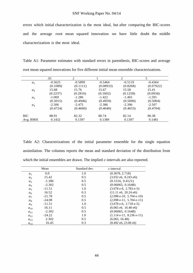
SNF Working Paper No. 04/14
44
errors which initial characterization is the most ideal, but after comparing the BIC-scores
and the average root mean squared innovation we have little doubt the middle
characterization is the most ideal.
Table A1: Parameter estimates with standard errors in parenthesis, BIC-scores and average
root mean squared innovations for five different initial mean ensemble characterizations.
.01 .1 1 2 5
-0.5625
(0.1089)
-0.5899
(0.1111)
-0.5464
(0.08933)
-0.5119
(0.8268)
-0.4364
(0.07922)
15.68
(0.2237)
15.76
(0.2816)
15.67
(0.1602)
15.58
(0.1258)
15.41
(0.0934)
-1.069
(0.5015)
-1.286
(0.4946)
-1.422
(0.4959)
-1.465
(0.5000)
-1.591
(0.5004)
-2.506
(0.4724)
-2.475
(0.4660)
-2.386
(0.4640)
-2.396
(0.4653)
-2.507
(0.4704)
BIC 88.91 82.32 80.74 82.14 90.38
Avg. RMSI 0.1432 0.1397 0.1389 0.1397 0.1481
Table A2: Characterizations of the initial parameter ensemble for the single equation
assimilation. The columns reports the mean and standard deviation of the distribution from
which the initial ensembles are drawn. The implied -intervals are also reported.
Mean Standard dev. -interval
0.0 1.0 (0.3678, 2.718)
15.42 0.5 (3.032 e6, 8.243 e6)
-1.386 0.5 (0.1516, 0.4121)
-2.302 0.5 (0.06065, 0.1648)
-11.51 1.0 (3.678 e-6, 2.783 e-5)
16.52 0.3 (11.11 e6, 20.24 e6)
-21.78 0.5 (2.098 e-10, 5.704 e-10)
-24.08 0.5 (2.098 e-11, 5.704 e-11)
-11.51 1.0 (3.678 e-6, 2.718 e-5)
16.11 0.5 (6.065 e6, 16.48 e6)
-2.302 0.5 (0.06065, 0.1648)
-24.22 1.0 (1.114 e-11, 8.236 e-11)
2.302 0.5 (6.065, 16.48)
16.45 0.3 (8.492 e6, 23.08 e6)

ARBEIDSNOTATWORKING PAPER04/14
The Ensemble Kalman Filter for Multidimensional Bioeconomic Models
Sturla F. KvamsdalLeif K. Sandal
To serve the needs for integrating economic considerations into management decisions in ecosystem frameworks, we need to build models that capture observed system dynamics and incorporate existing knowledge of eco systems while at the same time serve the needs of economics analysis. The main constraint for models to serve in economic analysis is dimensionality. In addition, models should be stable in order to apply in long-term management analysis. We use the ensemble Kalman filter to fit relatively simple models to ecosystem or foodweb data and estimate parameters that are stable over the observed variability in the data. The filter also provides a lower bound on the noise terms that a stochastic analysis require. In the present article, we apply the filter to model the main interactions in the Barents Sea ecosystem.
Helleveien 30 NO-5045 BergenNorway
P +47 55 95 95 00E [email protected] snf.no
Trykk: Allkopi Bergen
Samfunns- og næringslivsforskning ASCentre for Applied Research at NHH
Samfunns- og næringslivsforskning ASCentre for Applied Research at NHH


![Combining analog method and ensemble data assimilation ......The Analog Ensemble Kalman Filter and Smoother 5 [7]. Here, we exploit the low-computational ensemble Kalman recursions](https://img.dokumen.tips/doc/110x75/60ba54885e0f0a256565f9d9/combining-analog-method-and-ensemble-data-assimilation-the-analog-ensemble.jpg)