Two-Phase Time Synchronization-Free Localization Algorithm

Two-Phase Time Synchronization-Free Localization Algorithm for Underwater Sensor Networks Junhai Luo and Liying Fan

School of Electronic Engineering, University of Electronic Science and Technology of China, Chengdu,

Sichuan, 610073 China; [email protected]; [email protected]

* Correspondence: [email protected]

Abstract: Underwater Sensor Networks (UWSNs) can enable a broad range of applications such as resource monitoring, disaster prevention, and navigation-assisted. It is especially relevant for sensor nodes location in UWSNs. Global Positioning System (GPS) is not suitable for using in UWSNs because of the underwater propagation problems. Hence some localization algorithms based on the precise time synchronization between sensor nodes have been proposed which are not feasible for UWSNs. In this paper, we propose a localization algorithm called Two-Phase Time Synchronization-Free Localization Algorithm (TP-TSFLA). TP-TSFLA contains two phases, namely, range-based estimation phase and range-free evaluation phase. In the first phase, we address a time synchronization-free localization scheme base on the Particle Swarm Optimization (PSO) algorithm to decrease the localization error. In the second phase, we propose a Circle-based Range-Free Localization Algorithm (CRFLA) to locate the unlocalized sensor nodes which cannot obtain the location information through the first phase. In the second phase, sensor nodes which are localized in the first phase act as the new anchor nodes to help realize localization. Hence in this algorithm, we use a small number of mobile beacons to help achieve location without any other anchor nodes. Besides, to improve the precision of the range-free method, an extension of CRFLA by designing a coordinate adjustment scheme is updated. The simulation results show that TP-TSFLA can achieve a relative high localization ratio without time synchronization.

Keywords: Underwater sensor networks; synchronization-free; range-free; particle swarm optimization

1. Introduction

Underwater Sensor Networks (UWSNs) are usually composed of some autonomous and individual sensor nodes [1], which can sense data, perform computations intelligently, and forward information. Sensor nodes are spatially distributed in UWSNs with some sensing work to obtain water-related properties such as mass, temperature and pressure data [2]. UWSNs usually arrange many sensor nodes to monitor the underwater environment through the underwater acoustic communication to exchange the node location information and other data. UWSNs can be applied to many areas such as disaster early warning, pollutant control, marine resource exploration and maritime military.

The coordinates of the node location information In UWSNs are necessary to provide users with an efficient testing service. Therefore, underwater sensor node positioning can be regarded as the foundation and core for UWSNs. How to accurately estimate the position of the underwater node in UWSNs is of great research significance. Many researchers have reported the research results of localization. In outdoor environments, GPS-based positioning systems

Preprints (www.preprints.org) | NOT PEER-REVIEWED | Posted: 13 March 2017 doi:10.20944/preprints201703.0070.v1

Peer-reviewed version available at Sensors 2017, 17, 726; doi:10.3390/s17040726

http://dx.doi.org/10.20944/preprints201703.0070.v1

http://dx.doi.org/10.3390/s17040726

2 of 4

are used most and have good performance. In the indoor environment, RF-based or VLC-based positioning systems have attracted many researchers. However, they all not feasible to apply to UWSNs. RF signals only at low frequencies of about 30-300Hz can be used in the UWSNs, while requiring large antennas or high transmission power [3]. Optical signals are also subject to underwater attenuation and scattering [4]. Fortunately, the frequency of sound waves is little between 10Hz and 1MHz [1], which can provide small bandwidth but with long wavelengths. Therefore acoustics can be used to relay information over kilometers [5].

Underwater localization usually requires some objects with known locations (anchors) and objects to be localized (unknown nodes) [6]. The location information of anchors can be obtained through a variety of methods. In [7], the authors divide the localization scheme of UWSNs into two phases, namely the position-related information collection phase and the position estimation phase. In the first phase, position-related information such as the distance, angle, and hop count between each other or the anchor point is measured by the node. In the second phase, the localization algorithms are performed by the localized nodes or locally calculated by them. Conventional localization algorithms use the distance or angle measurements between the anchor and the unknown nodes to estimate the location of unknown nodes. Some positioning schemes do not require an anchor node and use the connection information to obtain the location of unknown nodes [8] [9]. The deployment of UWSNs is still a challenging task because of the limitations of computing power, cost, memory, transmission range and most of the lifetime of any single sensor [1]. A large number of anchor nodes can provide greater coverage and higher accuracy but may add cost. Therefore, how to decrease the number of anchor nodes or to achieve anchor-free localization is still a research direction. Moreover, the battery resources are limited to shorten the operation time. Thus, an effective strategy can guarantee the system performance with the low energy consumption. Many factors, such as water temperature, signal attenuation, dynamics, noise, may affect the performance.

The time synchronization is directly assumed in many localization schemes. However, it is not feasible in the real UWSNs. Then how to lose the time synchronization requirement or to develop a synchronization-free algorithm is a direction to solve this problem. In this paper, basing on the time synchronization-free localization using mobile beacons (we called it as TSFL) [10], we provide the Two-phase Time Synchronization-Free Algorithm (TP-TSFLA). TP-TSFLA can be divided into two phase, namely, range-based estimation phase (Phase I) and range-free evaluation phase (Phase II). In Phase I, we improve the TSFL algorithm based on the PSO algorithm to decrease the localization error. In Phase II, we propose a range-free algorithm to locate the unlocalized sensor nodes. Only sensor nodes which cannot be localized in Phase I can be processed in Phase II. In this phase, the localized sensor nodes are looked like the new anchor nodes to help realize localization. The unlocalized sensor node actively initiates a localization request, then the localized sensor node within the transmission range of the unlocalized sensor node can receive the request and respond their coordinate to the unlocalized node. Then the unlocalized sensor node starts a Circle-based Range-Free Localization Algorithm (CRFLA) to locate itself. Besides, a coordinate adjustment scheme is proposed to improve the precision of CRFLA.

The remaining portion of the paper is organized as follows. In Section II, we survey the localization algorithms according to the different natures. The system model is given in Section III. In Section IV, we use the PSO algorithm to improve the TSFL algorithm. CRFLA and its coordinate adjustment scheme are presented in Section V and Section VI respectively. The detailed algorithm procedure is shown in Section VII. Section VIII shows the simulation results and comparison. Finally, we conclude in Section IX.




http://dx.doi.org/10.3390/s17040726

3 of 4

2. Related Work

Recently, numerous localization algorithms have been put forward, and some researchers have done some survey of the localization algorithms [11-14].We discuss the localization algorithms in UWSNs in the following five aspects, namely computation algorithm, anchor requirement, range measurement, synchronization requirement, and communication between nodes. We only discuss the difference in each aspect and use some references to describe it.

According to the computation algorithm to be implemented, we classify the computation algorithms into two categories as centralized techniques [15] and distributed methods [16]. The centralized technology performs the localization algorithm at the command center or sink node. However, in the distributed method, the sensor node alone estimates the location of each sensor node. In [17] [18], a Reverse Localization Scheme (RLS) with a fast response to events is proposed. The scheme is based on the centralized technique. Thus, the data can be transmitted to the station, and the positioning algorithm is performed there. The scheme is described as two phases, namely, a transmitting phase and a centralized geometric localization phase. In the transmission phase, a new message exchange mechanism based on event-driven reporting is proposed. At the beginning of the second phase, the sink collects information from the anchor and estimates the location of the sensor node. The authors of [19] have shown a localization algorithm based on distributed technology. The authors mainly consider the problem of estimating the isolated unknown nodes and propose a Multihop Fitting Localization Approach (MFLA). The method sets the intermediate node between the beacon and the unknown node as a router to construct the path through the greedy method, and then fits the multi-hop path into a straight line and estimates it by trilateration.

The anchor requirement means the anchor node is required or not in the localization algorithm. According to this, we classify the localization algorithms into two taxonomies: anchor-free and anchor-based schemes. In UWSNs, many positioning algorithms can use anchor nodes to help estimate location. Because of the different localization algorithms, anchor nodes are not necessary, and some researchers have proposed a self-localization algorithm that does not need anchor nodes. The positioning scheme [20] is an anchor-based scheme. This scheme consists of four types of nodes, surface buoys, Detachable Elevator Transceivers (DETs), anchor nodes and ordinary nodes. Besides, the scheme locates the nodes in two phases. First, the anchor node uses a range-based distributed approach, the LSM, to locate itself. Secondly, ordinary nodes use the regional positioning scheme to achieve location-free centralized approach. In [21], an Anchor-Free Location Algorithm (AFLA) for active restricted UWSNs is proposed. The algorithm uses the relationship between adjacent nodes. In this scenario, the underwater sensor node actively limited means that when anchored to the seafloor, it floats in the sea and moves within the hemispherical region. A node with unknown location broadcasts a message and receives the information of other nodes at the same time. When the node receives two messages from two different nodes, it starts the location calculation process.

Based on the range measurement, we classify the localization algorithms into two categories, the range-based scheme, and the range-free scheme. In general, range-based schemes estimate distances by various algorithms and then convert them into positional information. The range-free scheme does not require distance measurement and bearing information, uses a local topology and the position of the neighboring anchor nodes to obtain the position estimate. However, the range-free scheme can only get a rough location with little accuracy. The positioning method of [22] is a range-based approach, and is called the multi-stage AUV-assisted positioning scheme that is an improvement of the "multi-stage DNR" scheme. In [22], the DNR is replaced by AUV. The AUV with known coordinates dives to a




http://dx.doi.org/10.3390/s17040726

4 of 4

pre-programmed depth and begins to traverse the sensor network after the preprogrammed path. When a non-collinear position receives three beacons, the triangulation is used to obtain the position of the node. In [23], the authors propose an efficient Area Localization Scheme (ALS). The scheme estimates the position of the sensor within a particular region. An anchor node broadcasts a beacon signal to a sensor node and sends an acoustic signal at a varying power level. The sensors passively monitor the signals and record the received information. A sensor node at a particular location can receive this property of different levels of signals from the same anchor node, the sensor measures its signal coordinates and stores the information, and then forward to the sink. The sink then uses the information gathered from sensor nodes to estimate the area in which the sensor is localized.

Synchronization requirement means that time synchronization is required or not in the localization algorithm. Based on this, we classify the localization algorithms into two categories: synchronization localization scheme and the synchronization-free localization scheme. In many cases, the localization scheme directly assumes that sensor nodes are synchronized with each other. However, this is difficult to implement in underwater environments, so the researchers have proposed some localization algorithms without synchronization requirements. The localization scheme of [24] requires time synchronization, but dual hydrophones on each node can reduce the need for time synchronization. In [24], a Dual Hydrophone Localization (DHL) approach is proposed, and the localization problem is converted to a half-plane intersection problem. As for the non-synchronized positioning scheme, we introduce three papers to show it. In [25] [26], a range-free scheme using AUV periodically broadcasts message blocks via four directional beams to estimate the location information of sensor nodes. The node receives the message block and uses two different continuous beams to estimate the position of the AUV at two different moments. The location of the nodes can then be obtained using two estimated locations. In [27], a Basic Synchronization-Free Localization (BSFL) scheme is proposed. It consists of two steps, namely the range difference calculation, and the position calculation. However, the BSFL still suffers from some drawbacks of the large-scale UWSNs. Therefore, a Large-Scale Localization Scheme (LSLS) based on BSFL is designed. It consists of three phases, namely sea surface anchoring, iterative localization and complementary phases.

Based on the communication characteristics between the reference node and the common node, we classify the UWSNs localization algorithm into two classes, single stage method [28-30] and multi-stage method [31-33]. The single stage means that the exchange of messages between all sensor nodes and the reference nodes is straightforward. After obtaining the location, they are still passive and cannot be used to help locate other sensor nodes [34]. In the multi-stage scheme, the common node does not need to communicate directly with the reference node. Once sensor nodes are localized, they become new reference nodes and can help to locate other sensor nodes [34]. The positioning scheme of [35] is based on a single-stage method. The authors use hyperbolic methods and normal distribution estimation error modeling and calibration for location estimation. The positioning scheme [36] is based on a multi-level localization scheme. The Top-down Positioning Scheme (TPS) for UWSNs without evenly distributed anchor nodes or additional infrastructures can increase location coverage while maintaining low positioning errors. In this scheme, there are three types of nodes, namely surface anchor nodes, new reference nodes, and nonlocalized nodes. First, only sensor nodes that are close to the surface anchor nodes can be localized. Once the positions of sensor nodes are obtained, they compute their confidence values and compare them to the confidence thresholds. If the node's confidence values are greater than the confidence thresholds, they become new reference nodes to help the non-localization nodes locate themselves.




http://dx.doi.org/10.3390/s17040726

5 of 4

3. System Model

3.1. Overview of the system

This paper mainly concentrates on locating the underwater sensor nodes. Due to the assumption of perfect time synchronization being unfeasible, in TP-TSFLA proposed in this paper, sensor nodes are randomly deployed in the different depth of the underwater to monitor the various areas. We assume sensor nodes are static for the 3D-network architecture. The pressure sensor is equipped on every sensor node to obtain the depth of the sensor node as the z-coordinate. Obtaining the x-coordinate and y-coordinate of the sensor node is necessary. Hence the 3D-localization problem can be transformed into a 2D-localization issue.

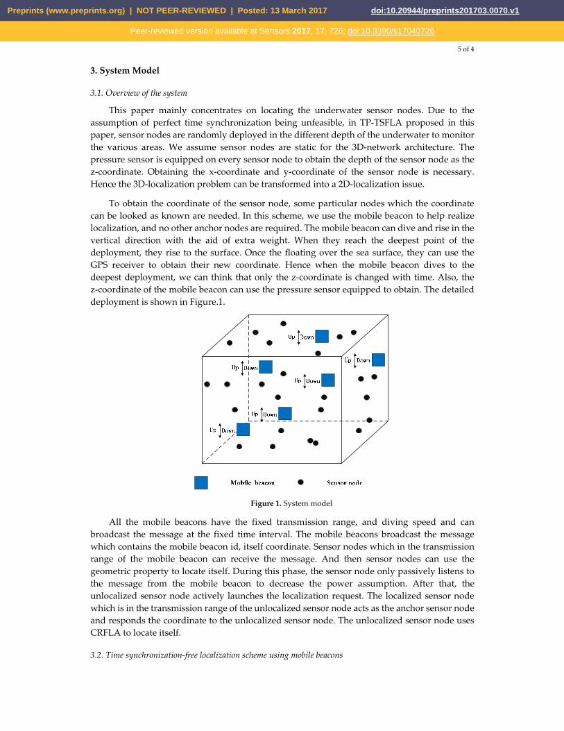
To obtain the coordinate of the sensor node, some particular nodes which the coordinate can be looked as known are needed. In this scheme, we use the mobile beacon to help realize localization, and no other anchor nodes are required. The mobile beacon can dive and rise in the vertical direction with the aid of extra weight. When they reach the deepest point of the deployment, they rise to the surface. Once the floating over the sea surface, they can use the GPS receiver to obtain their new coordinate. Hence when the mobile beacon dives to the deepest deployment, we can think that only the z-coordinate is changed with time. Also, the z-coordinate of the mobile beacon can use the pressure sensor equipped to obtain. The detailed deployment is shown in Figure.1.

Figure 1. System model

All the mobile beacons have the fixed transmission range, and diving speed and can broadcast the message at the fixed time interval. The mobile beacons broadcast the message which contains the mobile beacon id, itself coordinate. Sensor nodes which in the transmission range of the mobile beacon can receive the message. And then sensor nodes can use the geometric property to locate itself. During this phase, the sensor node only passively listens to the message from the mobile beacon to decrease the power assumption. After that, the unlocalized sensor node actively launches the localization request. The localized sensor node which is in the transmission range of the unlocalized sensor node acts as the anchor sensor node and responds the coordinate to the unlocalized sensor node. The unlocalized sensor node uses CRFLA to locate itself.

3.2. Time synchronization-free localization scheme using mobile beacons




http://dx.doi.org/10.3390/s17040726

6 of 4

Basing on the system model, we can employ the time synchronization-free localization scheme using mobile beacons proposed by the authors of [10] to locate sensor nodes in Phase I. Hence to describe it concisely, we called it as TSFL algorithm. The mobile beacon dives and

rises in the underwater at the fixed speed 1v . 1T and 2T express the time that the first message received by sensor node and the second message received by the sensor node respectively.

Hence the coordinate of the mobile beacon at the different time is denoted as ),,( 111 zyx and ),,( 211 zyx . The speed of sound is 2v , and the coordinate of the senor node is ),,( 3zyx .

If 231 zzz << , we can obtain the distance d , and the detailed process can be found in [10].

21

2

11

1

4

1HB

B

Ad −

+

= , (1)

where 12 zzH −= , 131 zzH −= , 322 zzH −= ,22

211 HHA −= , and 12 TTT −=Δ ,

Δ−= T

v

HvB1

21.

If , we can obtain the distance d ,

2

2

22

2

4

1HB

B

Ad −

+

= , (2)

321 zzz << where 13 zzH −= , 121 zzH −= , 232 zzH −= ,22

22 HHA −=, and

Δ−= T

v

HvB1

122

.

If 213 zzz << , we can obtain the distance d ,

21

2

33

3

4

1HB

B

Ad −

+

= , (3)

where 32 zzH −= , 311 zzH −= , 122 zzH −=22

12 HHA −=and

Δ−= T

v

HvB1

222

.

If at least three distance measures from different mobile beacons have been obtained, the position of the sensor node can be obtained.

However, the authors do not take the impact of the water current into account and make the speed of the mobile beacon and sound as a constant. It is not reality. Thus we consider the error caused by the underwater environment and propose localization scheme based on the PSO algorithm. Besides, to save the cost, the number of the mobile beacon is limited which leads to the lower localization ratio. Primarily we use the algorithm into the relatively large environment. Hence we improve the algorithm based on the two aspects in TP-TSFLA.

3.3. Algorithm Features

In this paper, TP-TSFLA is mainly concerned about the time synchronization requirements, trying to find a synchronization-free localization scheme. The localization algorithm proposed in this paper is based on the distributed localization technique. In Phase I, mobile beacons are used as anchor nodes, and in Phase II, sensor nodes that are localized in the first phase act as




http://dx.doi.org/10.3390/s17040726

7 of 4

anchors to help locate the unlocalized sensor nodes. The algorithm used in Phase I is range-based, while the algorithm of Phase II is range-free, and belongs to the multi-stage method.

The features of the system can be described as follows.

• The system is suitable to use in the 3D-network architecture, and the sensor node is assumed static in the network. Every sensor node is equipped with a pressure sensor to sense the depth of the sensor node. The mobile beacon can obtain the x-coordinate and y-coordinate by GPS, and only the z-coordinate is changed when the mobile beacon dives to the sea.

• The diving speed of the mobile beacon and the rate of the sound in the water of the TSFL algorithm are assumed as a constant. The mobile beacon broadcasts the message in the fixed interval. The transmission range of the mobile beacon and sensor node is fixed. The transmission range of the mobile beacon is larger than the transmission range of sensor node.

• During Phase I, sensor nodes passively listen to the mobile beacon, not transmitting a message to the mobile beacon to decrease the power assumption. While in Phase II, sensor nodes can initiate active communication with other sensor nodes to obtain the message which is required to realize localization.

• In TP-TSFLA, the small number of the mobile beacons are used as the anchor nodes. In Phase II, the algorithm uses the multi-stage scheme to help realize the localization. The localized sensor nodes are used as the new anchor nodes.

4. Range-based Estimation Algorithm of Using PSO

In this section, we employ the Particle Swarm Optimization (PSO) algorithm to improve the precision of the estimated position. To solve a variety of optimization problems, many optimization algorithms have been proposed, such as climbing method, genetic algorithm and so on. Hill climbing method has high precision, but it is easy to fall into the local minimum. Genetic algorithm belongs to the evolutionary algorithm. However, the genetic algorithm requires more sophisticated programming, the choice of these parameters severely affect the quality of the solution, and most of these parameters depend on experience. The PSO algorithm, with smooth implementation, high precision, and fast convergence has similarly to a genetic algorithm, and it is also starting from the random solution. The PSO algorithm iteratively finds the optimal solution, and it evaluates the quality of the solution through fitness, but it is simpler than the genetic algorithm. It does not have the "cross" (Crossover) and "mutation." The global optimum is sought by following the current search to the optimal value.

Basing on TSFL, after at least three distance measures from different mobile beacons have been obtained, the authors obtain the estimated position of the sensor node using the following formula

( ) bAAAy

xX TT 1

ˆ

ˆ −=

= , (4)

where




http://dx.doi.org/10.3390/s17040726

8 of 4

=

−−−−

−−

−−

)(2)(2

)(2)(2

)(2)(2

11

22

11

nnnn

nn

nn

yyxx

yyxx

yyxx

A

, (5)

and

−+−−−

−+−−−

−+−−−

=

−−−222

12

122

1

2222

22

222

2221

21

221

nnnnnn

nnn

nnn

yxyxdd

yxyxdd

yxyxdd

b

, (6)

In our algorithm, we extend the estimated position of the sensor node )ˆ,ˆ( yx to two

dimension area. The x-coordinate of the particle is between ax −ˆ and ax +ˆ , and y-coordinate is between by −ˆ and by +ˆ shown as

]ˆ,ˆ[ axaxxj +−∈ , (7)

]ˆ,ˆ[ bybyyj +−∈ , (8)

where a and b are constants to determine the range of the solution-space. ),( jj yx are the

coordinates of the particle. Hence we initialize a group of random particles (random

candidate solution) in the rectangular area. And then the PSO algorithm iteratively finds the

optimal solution. In each iteration, the particle updates itself by tracking two "extremum".

The first is the optimal solution found by the particle itself, and the solution is called the

individual extreme (pBest). The other extremum is the optimal solution found by the whole

population. The extreme value is the global extreme value (gBest). When these two optimal

values are found, the particle updates its speed and new position according to the following

formula

[])[](*()*2

[])[](*()*1[]*[]

presentgbestrandc

presentpbestrandcvwv

−+−+=

, (9)

[][][] vpresentprsent += , (10)

where []v is the speed of the particle, w is the inertia weight, []present is the current

position of the particle, []pbest is the individual extreme value, [ ]gbest is the global

extreme value, and ()rand is the random number between (0, 1). 1c and 2c are the

learning factor.




http://dx.doi.org/10.3390/s17040726

9 of 4

Fitness Function: the distance of unknown sensor node ( )zyx ,, from the anchor node

( )iii zyx ,, expressed as ir is given as

=−+−+−

=−+−+−

=−+−+−

nnnn rzzyyxx

rzzyyxx

rzzyyxx

222

22

22

22

2

12

12

12

1

)()()(

)()()(

)()()(

, (11)

The coordinate of the particle is ( )jjj zyx ,, , the number of anchor node is N, and the fitness

function can be described as

=

−−+−+−=N

irzzyyxxf iijijijj

1

2)(2)(2)( , (12)

If the fitness function tends to 0, the result solution coordinate tends to be the coordinate of the unlocalized sensor node. After the maximum number of loops is reached, the current global extreme value will be chosen as the coordinate of the sensor node.

5. CRFLA

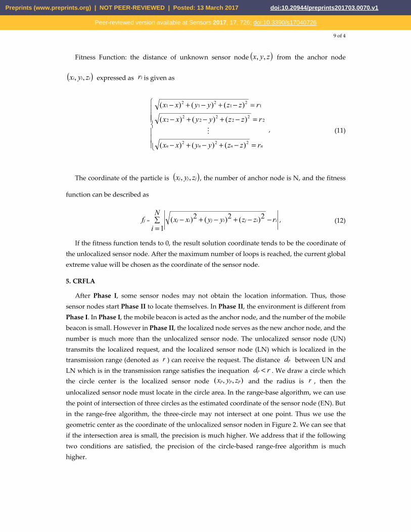
After Phase I, some sensor nodes may not obtain the location information. Thus, those sensor nodes start Phase II to locate themselves. In Phase II, the environment is different from Phase I. In Phase I, the mobile beacon is acted as the anchor node, and the number of the mobile beacon is small. However in Phase II, the localized node serves as the new anchor node, and the number is much more than the unlocalized sensor node. The unlocalized sensor node (UN) transmits the localized request, and the localized sensor node (LN) which is localized in the transmission range (denoted as r ) can receive the request. The distance pd between UN and LN which is in the transmission range satisfies the inequation rdp < . We draw a circle which the circle center is the localized sensor node ),,( ppp zyx and the radius is r , then the

unlocalized sensor node must locate in the circle area. In the range-base algorithm, we can use the point of intersection of three circles as the estimated coordinate of the sensor node (EN). But in the range-free algorithm, the three-circle may not intersect at one point. Thus we use the geometric center as the coordinate of the unlocalized sensor noden in Figure 2. We can see that if the intersection area is small, the precision is much higher. We address that if the following two conditions are satisfied, the precision of the circle-based range-free algorithm is much higher.




http://dx.doi.org/10.3390/s17040726

10 of 4

LN2

LN1

LN3

EN

The point of intersection of the three LNs

UN

EN LN UN

Figure 2. CRFLA

Condition I: the distance pd between the unlocalized sensor node and the localized sensor node infinitely closes to the transmission range r of the unlocalized sensor node.

Condition II: the three localized sensor nodes localize in the different direction of the circle.

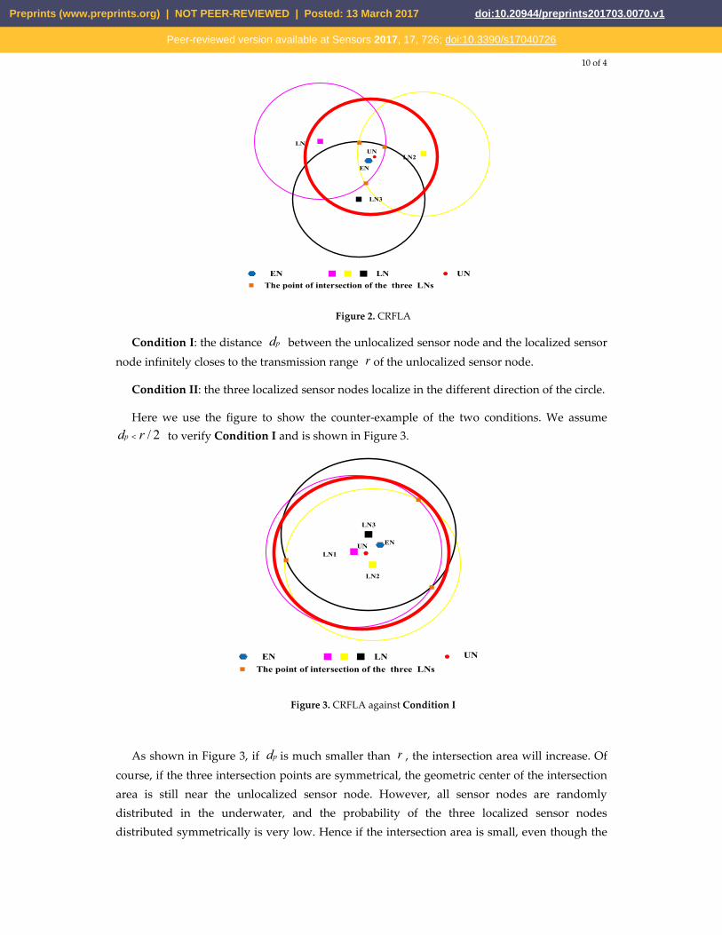
Here we use the figure to show the counter-example of the two conditions. We assume2/rdp < to verify Condition I and is shown in Figure 3.

LN2

LN1

LN3

ENUN


EN LN UN

Figure 3. CRFLA against Condition I

As shown in Figure 3, if pd is much smaller than r , the intersection area will increase. Of course, if the three intersection points are symmetrical, the geometric center of the intersection area is still near the unlocalized sensor node. However, all sensor nodes are randomly distributed in the underwater, and the probability of the three localized sensor nodes distributed symmetrically is very low. Hence if the intersection area is small, even though the




http://dx.doi.org/10.3390/s17040726

11 of 4

three localized sensor nodes are not symmetrical, the geometric center will not far away from the unlocalized sensor node.

To as far as possible satisfy Condition I, we employ the nature that the signal strength decreases with increasing distance. The unlocalized sensor node utilizes the response information of the localized sensor node which contains the coordinate of the localized sensor node and the signal strength to choose the three localized sensor nodes. Simply to say, the unlocalized sensor node determines the three localized nodes which the signal strength is lowest. It is to say the distance of the chosen three localized sensor nodes from the unlocalized sensor node is the largest in the all localized sensor nodes which can receive the information of the unlocalized sensor node. Here we do not obtain the distance from the signal strength but compare the value of the signal strength.

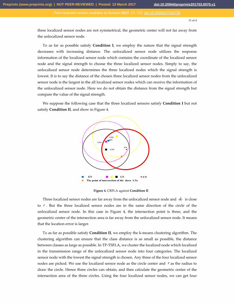
We suppose the following case that the three localized sensors satisfy Condition I but not satisfy Condition II, and show in Figure 4.

LN2

LN1

LN3

EN

UN


EN LN UN

Figure 4. CRFLA against Condition II

Three localized sensor nodes are far away from the unlocalized sensor node and pd is close to r . But the three localized sensor nodes are in the same direction of the circle of the unlocalized sensor node. In this case in Figure 4, the intersection point is three, and the geometric center of the intersection area is far away from the unlocalized sensor node. It means that the location error is larger.

To as far as possible satisfy Condition II, we employ the k-means clustering algorithm. The clustering algorithm can ensure that the class distance is as small as possible, the distance between classes as large as possible. In TP-TSFLA, we cluster the localized node which localized in the transmission range of the unlocalized sensor node into four categories. The localized sensor node with the lowest the signal strength is chosen. Any three of the four localized sensor nodes are picked. We use the localized sensor node as the circle center and r as the radius to draw the circle. Hence three circles can obtain, and then calculate the geometric center of the intersection area of the three circles. Using the four localized sensor nodes, we can get four




http://dx.doi.org/10.3390/s17040726

12 of 4

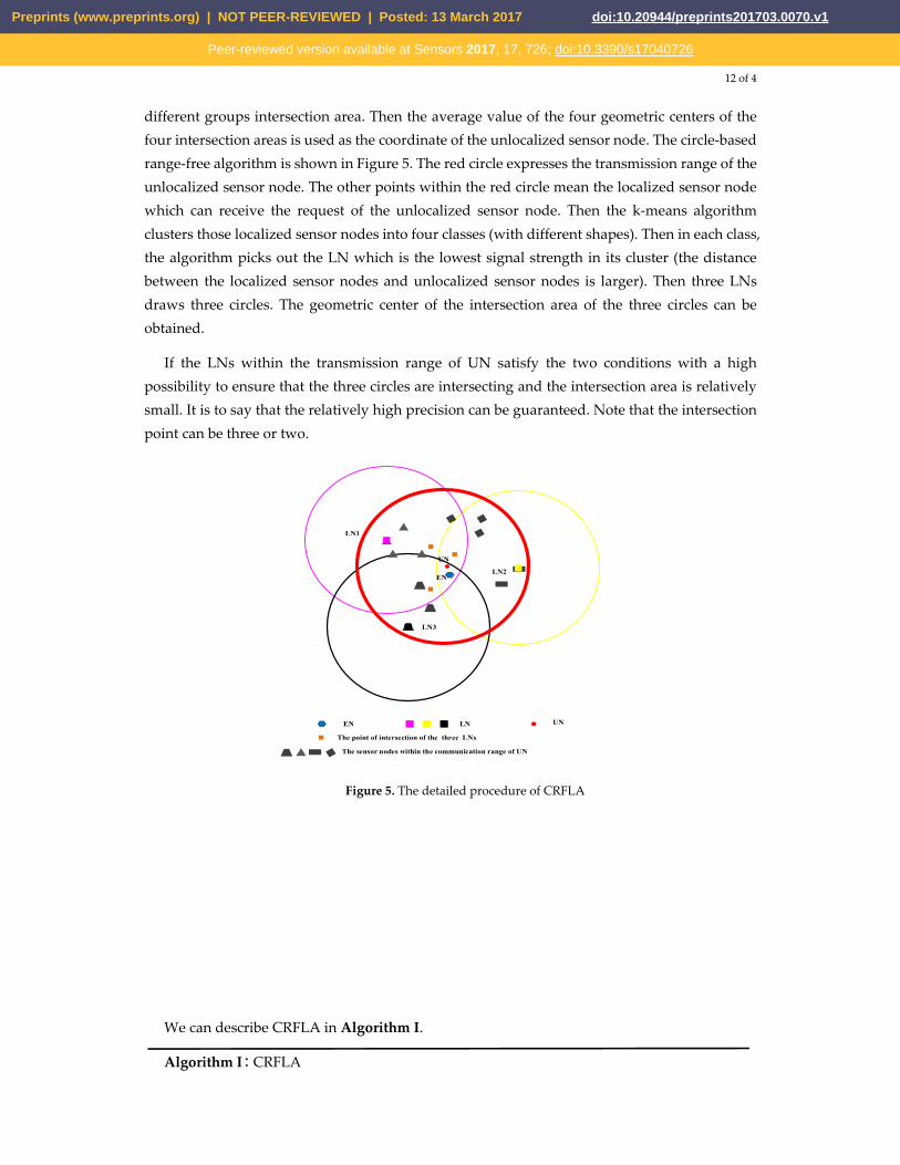
different groups intersection area. Then the average value of the four geometric centers of the four intersection areas is used as the coordinate of the unlocalized sensor node. The circle-based range-free algorithm is shown in Figure 5. The red circle expresses the transmission range of the unlocalized sensor node. The other points within the red circle mean the localized sensor node which can receive the request of the unlocalized sensor node. Then the k-means algorithm clusters those localized sensor nodes into four classes (with different shapes). Then in each class, the algorithm picks out the LN which is the lowest signal strength in its cluster (the distance between the localized sensor nodes and unlocalized sensor nodes is larger). Then three LNs draws three circles. The geometric center of the intersection area of the three circles can be obtained.

If the LNs within the transmission range of UN satisfy the two conditions with a high possibility to ensure that the three circles are intersecting and the intersection area is relatively small. It is to say that the relatively high precision can be guaranteed. Note that the intersection point can be three or two.

LN2

LN1

LN3

EN

UN

The sensor nodes within the communication range of UN


EN LN UN

Figure 5. The detailed procedure of CRFLA

We can describe CRFLA in Algorithm I.

Algorithm I：CRFLA




http://dx.doi.org/10.3390/s17040726

13 of 4

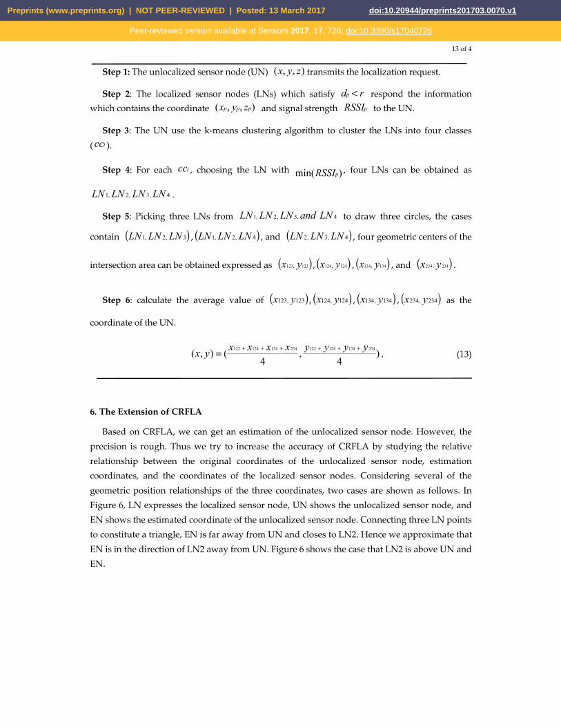
Step 1: The unlocalized sensor node (UN) ),,( zyx transmits the localization request.

Step 2: The localized sensor nodes (LNs) which satisfy rdp < respond the information which contains the coordinate ),,( ppp zyx and signal strength pRSSI to the UN.

Step 3: The UN use the k-means clustering algorithm to cluster the LNs into four classes ( icc ).

Step 4: For each icc , choosing the LN with )min( pRSSI , four LNs can be obtained as

4,3,2,1 LNLNLNLN .

Step 5: Picking three LNs from 1, 2, 3, 4 LN LN LN and LN to draw three circles, the cases

contain ( )3,2,1 LNLNLN , ( )4,2,1 LNLNLN , and ( )4,3,2 LNLNLN , four geometric centers of the

intersection area can be obtained expressed as ( )123123, yx , ( )124124, yx , ( )134134, yx , and ( )234234, yx .

Step 6: calculate the average value of ( )123,123 yx , ( )124,124 yx , ( )134,134 yx , ( )234,234 yx as the

coordinate of the UN.

)4

,4

(),(234134124123234134124123 yyyyxxxx

yx++++++= , (13)

6. The Extension of CRFLA

Based on CRFLA, we can get an estimation of the unlocalized sensor node. However, the precision is rough. Thus we try to increase the accuracy of CRFLA by studying the relative relationship between the original coordinates of the unlocalized sensor node, estimation coordinates, and the coordinates of the localized sensor nodes. Considering several of the geometric position relationships of the three coordinates, two cases are shown as follows. In Figure 6, LN expresses the localized sensor node, UN shows the unlocalized sensor node, and EN shows the estimated coordinate of the unlocalized sensor node. Connecting three LN points to constitute a triangle, EN is far away from UN and closes to LN2. Hence we approximate that EN is in the direction of LN2 away from UN. Figure 6 shows the case that LN2 is above UN and EN.




http://dx.doi.org/10.3390/s17040726

14 of 4

LN2

LN1

ENUN

α

LN3

EN LN UN


Figure 6. The localization relationship of the UN and EN when LN2 is above the UN and EN

The case that LN2 is below EN and UN is shown in Figure 7. Similarly, we can approximate that EN is in the direction of LN2 away from UN. Next, we should try to find out why the point is LN2, not LN1 or LN3. Through observation, we find the angle α is the largest angle in the triangle. Of course, just a lot of cases are tested, and maybe not all the cases are taken into account. But from those tests, it is true that it is high possibility that EN is in the direction of LN2 away from UN. Hence, LN2 corresponding to the point that the angle of it is the largest angle in the triangle. We transfer the largest angle to the longest opposite edge of angle. It means that the distance between N1 and LN3 is largest. We will use MATLAB simulation to demonstrate it. Next, we give the mathematical model of the extension of CRFLA.

UNLN3

LN1

LN2

EN

α

EN LN UN


Figure 7. The localization relationship of the UN and EN when LN2 is below the UN and EN

The coordinate of the UN is ),,( zyx , the coordinate of the LN2 is ),,( 222 zyx , and the coordinate of EN is )ˆ,ˆ,ˆ( zyx . If we want )ˆ,ˆ,ˆ( zyx is close to ),,( zyx , we should adjust the coordinate )ˆ,ˆ,ˆ( zyx in the opposite direction of the movement of EN that EN is in the direction

of LN2 away from UN. Because the z-coordinate can be obtained from the pressure sensor equipped on the unlocalized sensor node, we just discuss the adjustment of the x-coordinate




http://dx.doi.org/10.3390/s17040726

15 of 4

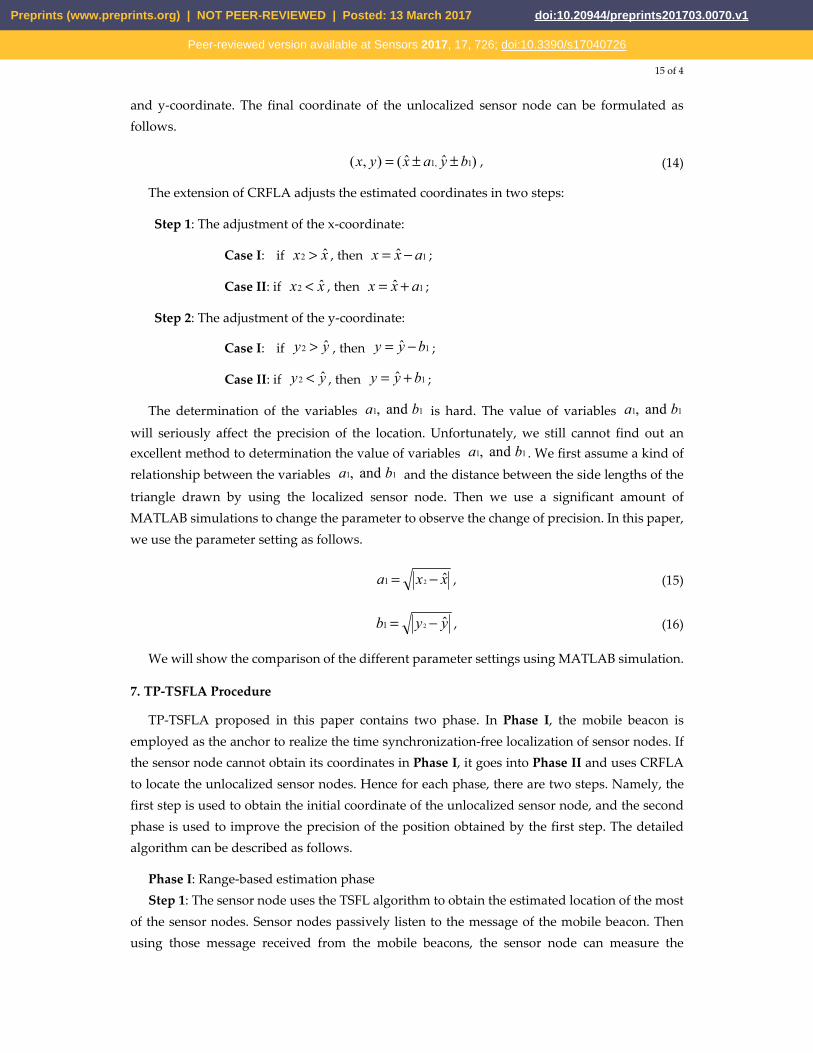
and y-coordinate. The final coordinate of the unlocalized sensor node can be formulated as follows.

)ˆˆ(),( 1,1 byaxyx ±±= , (14)

The extension of CRFLA adjusts the estimated coordinates in two steps:

Step 1: The adjustment of the x-coordinate:

Case I: if xx ˆ2 > , then 1ˆ axx −= ;

Case II: if xx ˆ2 < , then 1ˆ axx += ;

Step 2: The adjustment of the y-coordinate:

Case I: if yy ˆ2 > , then 1ˆ byy −= ;

Case II: if yy ˆ2 < , then 1ˆ byy += ;

The determination of the variables 1 1, and a b is hard. The value of variables 1 1, and a b

will seriously affect the precision of the location. Unfortunately, we still cannot find out an excellent method to determination the value of variables 1 1, and a b . We first assume a kind of relationship between the variables 1 1, and a b and the distance between the side lengths of the

triangle drawn by using the localized sensor node. Then we use a significant amount of MATLAB simulations to change the parameter to observe the change of precision. In this paper, we use the parameter setting as follows.

xxa ˆ21 −= , (15)

yyb ˆ21 −= , (16)

We will show the comparison of the different parameter settings using MATLAB simulation.

7. TP-TSFLA Procedure

TP-TSFLA proposed in this paper contains two phase. In Phase I, the mobile beacon is employed as the anchor to realize the time synchronization-free localization of sensor nodes. If the sensor node cannot obtain its coordinates in Phase I, it goes into Phase II and uses CRFLA to locate the unlocalized sensor nodes. Hence for each phase, there are two steps. Namely, the first step is used to obtain the initial coordinate of the unlocalized sensor node, and the second phase is used to improve the precision of the position obtained by the first step. The detailed algorithm can be described as follows.

Phase I: Range-based estimation phase Step 1: The sensor node uses the TSFL algorithm to obtain the estimated location of the most

of the sensor nodes. Sensor nodes passively listen to the message of the mobile beacon. Then using those message received from the mobile beacons, the sensor node can measure the




http://dx.doi.org/10.3390/s17040726

16 of 4

distance from the mobile beacon. If at least three distance measures are obtained, then sensor node use those distance measures to estimate their location.

Step 2: Every sensor node which has obtained the estimated location through Step 1 use the PSO algorithm to optimize the estimated position, and then the optimized estimated locations are taken as the final estimated location of the sensor node.

Phase II: Range-free evaluation phase Step 3: Sensor nodes which cannot obtain the position through Phase I actively launch the

localization request. The localized sensor nodes within the transmission range of the unlocalized sensor node receive the request and respond their coordinates to the sensor node. Then the unlocalized sensor node uses CRFLA to obtain its coordinate.

Step 4: Sensor nodes adjust the estimated coordinates to improve the precision of the range-free method, and the final estimated location is taken as the coordinate of the unlocalized sensor node.

The block diagram of TP-TSFLA is shown in Figure 8.

Sensor nodes

Mobile Beacons act as anchors

TSFL algorithm

PSO algorithm

Loci=0 Circle-based range free localization

algorithm

Loci=1

Revise method

Located sensor nodes act

as anchorsFinal location estimation of the

sensor nodes

Final location estimation of the

sensor nodes

Figure 8. Block diagram of TP-TSFLA

Table 1 gives all the mathematical notation and symbols definitions used of Algorithm II.

Table 1. Notation

Sign Meaning

iD Number of mobile beacons which the distance measurement from the sensor node i

jM The number of the message received from the j mobile beacon

iLoc If the node i is localized, the 1=iLoc , else 0=iLoc

3z The z-coordinate of the sensor node

)ˆ,ˆ(

_

yx

inicoor i The estimated coordinate of the sensor node i without using the optimized algorithm




http://dx.doi.org/10.3390/s17040726

17 of 4

),,( 3zyx

coordinatei The estimated coordinate of the sensor node i after using the optimized algorithm

jjf The fitness function of the particle jj

Maxgen Number of iterations

gbest The population optimal

),,( 222 zyx The coordinate of localized sensor node which corresponds to the point that the angle of it is the largest angle in the triangle

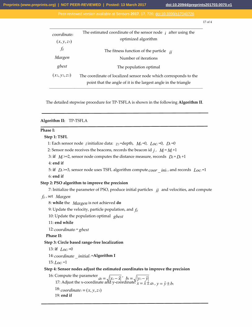
The detailed stepwise procedure for TP-TSFLA is shown in the following Algorithm II.

Algorithm II: TP-TSFLA

Phase I: Step 1: TSFL 1: Each sensor node i initialize data: 3z =depth, iiM =0, iLoc =0, iD =0 2: Sensor node receives the beacons, records the beacon id j , jM = jM +1

3: if jM >=2, sensor node computes the distance measure, records iD = iD +1 4: end if 5: if iD >=3, sensor node uses TSFL algorithm compute iinicoor _ , and records iLoc =1 6: end if

Step 2: PSO algorithm to improve the precision 7: Initialize the parameter of PSO, produce initial particles jj and velocities, and compute

jjf , set Maxgen 8: while the Maxgen is not achieved do 9: Update the velocity, particle population, and jjf 10: Update the population optimal gbest 11: end while 12: icoordinate = gbest

Phase II: Step 3: Circle based range-free localization

13: if iLoc =0 14: iinitialcoordinate _ =Algorithm I 15: iLoc =1

Step 4: Sensor nodes adjust the estimated coordinates to improve the precision 16: Compute the parameter

xxa ˆ21 −= , yyb ˆ21 −=

17: Adjust the x-coordinate and y-coordinate: 1ˆ axx ±= , 1ˆ byy ±= 18: ),,( 3zyxcoordinatei = 19: end if




http://dx.doi.org/10.3390/s17040726

18 of 4

8. Discussion

In this section, we use the MATLAB simulation to evaluate the performance of TP-TSFLA. The simulation environment is mmm 500600600 ×× , and 800 sensor nodes are deployed in UWSNs. All sensor nodes are looked as stationary. We use 25 mobile beacons in this environment. The following parameters are the same as the setting of [10]. The speed of sound is set to 1500m/s, and the rate of the mobile beacon is 1m/s. The beacon interval varies from the 30s to 100s, and the transmission range varies from 150m to 250m.

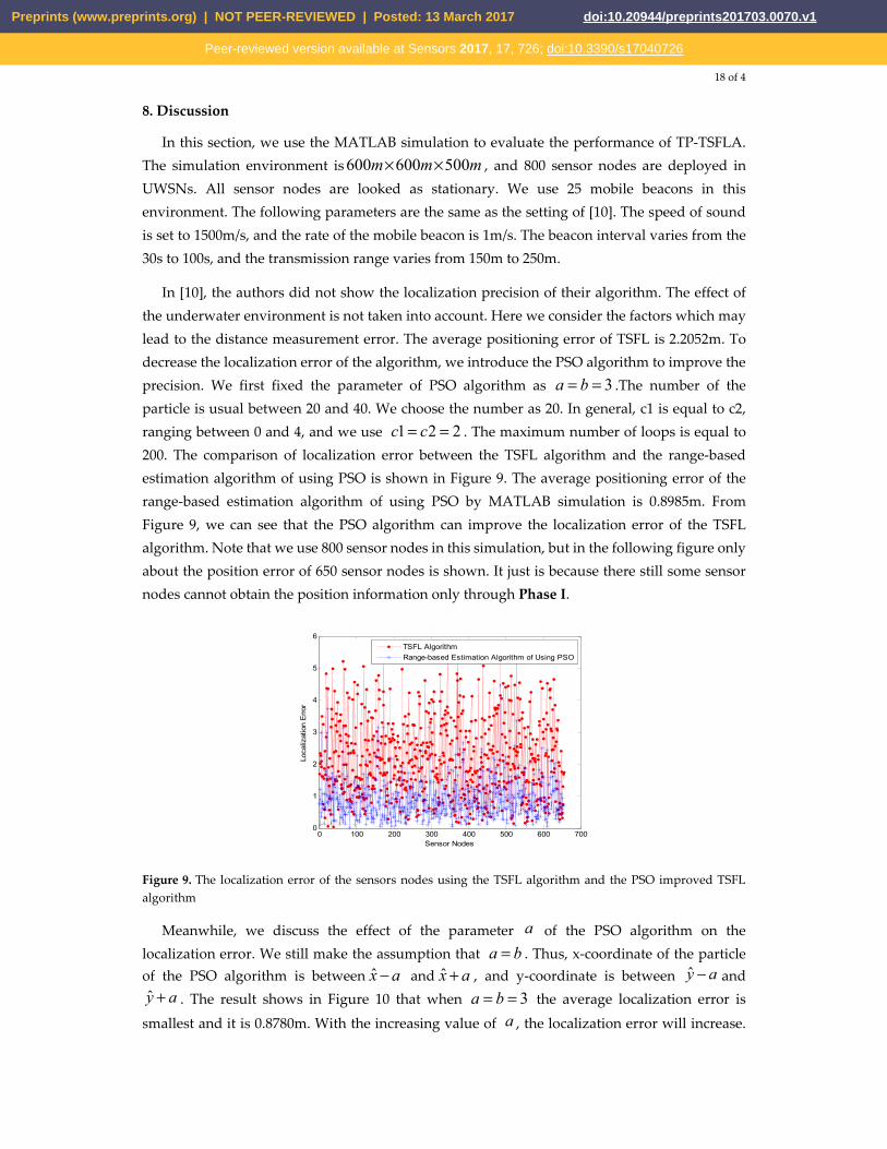
In [10], the authors did not show the localization precision of their algorithm. The effect of the underwater environment is not taken into account. Here we consider the factors which may lead to the distance measurement error. The average positioning error of TSFL is 2.2052m. To decrease the localization error of the algorithm, we introduce the PSO algorithm to improve the precision. We first fixed the parameter of PSO algorithm as 3== ba .The number of the particle is usual between 20 and 40. We choose the number as 20. In general, c1 is equal to c2, ranging between 0 and 4, and we use 221 == cc . The maximum number of loops is equal to 200. The comparison of localization error between the TSFL algorithm and the range-based estimation algorithm of using PSO is shown in Figure 9. The average positioning error of the range-based estimation algorithm of using PSO by MATLAB simulation is 0.8985m. From Figure 9, we can see that the PSO algorithm can improve the localization error of the TSFL algorithm. Note that we use 800 sensor nodes in this simulation, but in the following figure only about the position error of 650 sensor nodes is shown. It just is because there still some sensor nodes cannot obtain the position information only through Phase I.

Figure 9. The localization error of the sensors nodes using the TSFL algorithm and the PSO improved TSFL algorithm

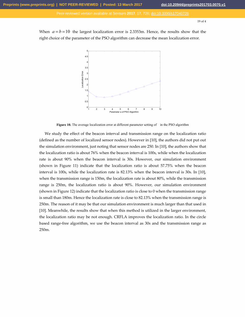
Meanwhile, we discuss the effect of the parameter a of the PSO algorithm on the localization error. We still make the assumption that ba = . Thus, x-coordinate of the particle of the PSO algorithm is between ax −ˆ and ax +ˆ , and y-coordinate is between ay −ˆ and

ay +ˆ . The result shows in Figure 10 that when 3== ba the average localization error is

smallest and it is 0.8780m. With the increasing value of a , the localization error will increase.

0 100 200 300 400 500 600 7000

1

2

3

4

5

6

Sensor Nodes

Loca

lizat

ion

Err

or

TSFL Algorithm

Range-based Estimation Algorithm of Using PSO




http://dx.doi.org/10.3390/s17040726

19 of 4

When 10== ba the largest localization error is 2.3353m. Hence, the results show that the right choice of the parameter of the PSO algorithm can decrease the mean localization error.

Figure 10. The average localization error at different parameter setting of in the PSO algorithm

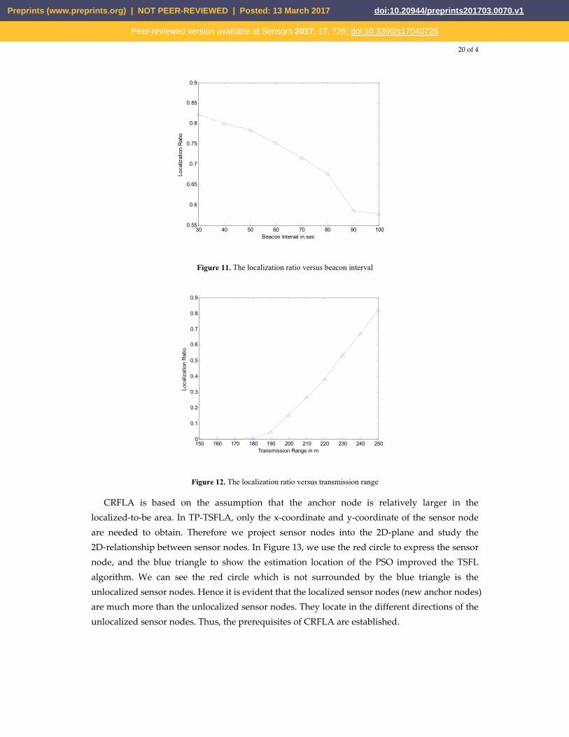
We study the effect of the beacon interval and transmission range on the localization ratio (defined as the number of localized sensor nodes). However in [10], the authors did not put out the simulation environment, just noting that sensor nodes are 250. In [10], the authors show that the localization ratio is about 76% when the beacon interval is 100s, while when the localization rate is about 90% when the beacon interval is 30s. However, our simulation environment (shown in Figure 11) indicate that the localization ratio is about 57.75% when the beacon interval is 100s, while the localization rate is 82.13% when the beacon interval is 30s. In [10], when the transmission range is 150m, the localization rate is about 80%, while the transmission range is 250m, the localization ratio is about 90%. However, our simulation environment (shown in Figure 12) indicate that the localization ratio is close to 0 when the transmission range is small than 180m. Hence the localization rate is close to 82.13% when the transmission range is 250m. The reason of it may be that our simulation environment is much larger than that used in [10]. Meanwhile, the results show that when this method is utilized in the larger environment, the localization ratio may be not enough. CRFLA improves the localization ratio. In the circle based range-free algorithm, we use the beacon interval as 30s and the transmission range as 250m.

1 2 3 4 5 6 7 8 9 100

0.5

1

1.5

2

2.5

3

3.5

4

4.5

5

Parameter a of PSO Algorithm

Loca

lizat

ion

Err

or




http://dx.doi.org/10.3390/s17040726

20 of 4

Figure 11. The localization ratio versus beacon interval

Figure 12. The localization ratio versus transmission range

CRFLA is based on the assumption that the anchor node is relatively larger in the localized-to-be area. In TP-TSFLA, only the x-coordinate and y-coordinate of the sensor node are needed to obtain. Therefore we project sensor nodes into the 2D-plane and study the 2D-relationship between sensor nodes. In Figure 13, we use the red circle to express the sensor node, and the blue triangle to show the estimation location of the PSO improved the TSFL algorithm. We can see the red circle which is not surrounded by the blue triangle is the unlocalized sensor nodes. Hence it is evident that the localized sensor nodes (new anchor nodes) are much more than the unlocalized sensor nodes. They locate in the different directions of the unlocalized sensor nodes. Thus, the prerequisites of CRFLA are established.

30 40 50 60 70 80 90 1000.55

0.6

0.65

0.7

0.75

0.8

0.85

0.9

Beacon Interval in sec

Loca

lizat

ion

Rat

io

150 160 170 180 190 200 210 220 230 240 2500

0.1

0.2

0.3

0.4

0.5

0.6

0.7

0.8

0.9

Transmission Range in m

Loca

lizat

ion

Rat

io




http://dx.doi.org/10.3390/s17040726

21 of 4

Figure 13. The location of the sensor node projected to the 2D-plane

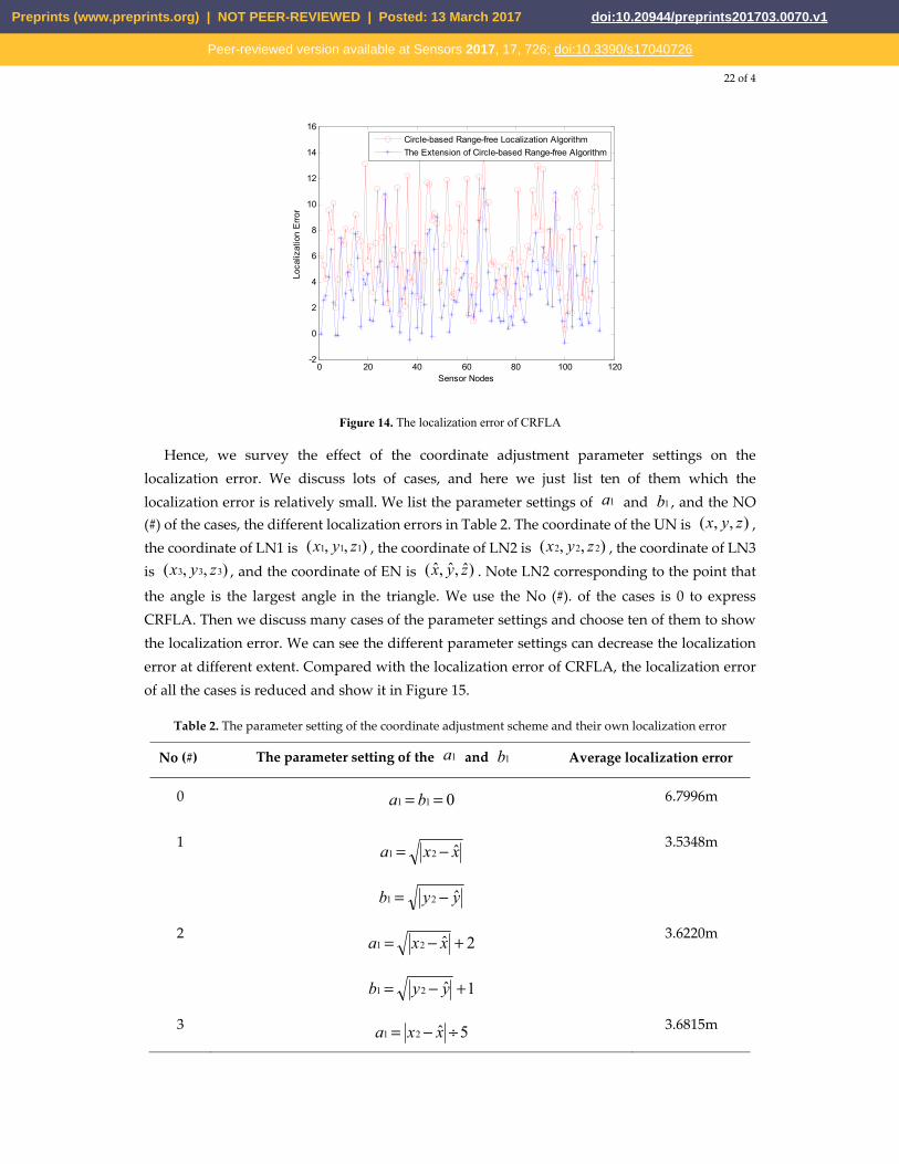
We then use MATLAB simulation to estimate the positioning error of CRFLA. The results show that the average positioning error is about 6.7996m. Compared with the range-based localization algorithm (Phase I), the localization error is much larger. It is the shortcoming of the range-free localization algorithm. But the range-free is much simple, and the power assumption is much lower. Besides the range-free localization does not need some unrealistic assumptions such as precise time synchronization, and fixed speed which may lead to the localization error. An extension of CRFLA is proposed by designing a coordinate adjustment scheme. The comparison of the localization error of the unlocalized sensor node in Phase II is shown in Figure 14. From Figure 14, we can see most of the localization error of the extension of CRFLA is lower than CRFLA. The average positioning error using the extension of CRFLA is 3.5348m. Besides, the extension of CRFLA may increase the localization error. But it is just a small part of it. Hence, to this extent, the coordinate adjustment scheme is useful. Compared with TSFL which those coordinates of unlocalized sensor node are unknown, TP-TSFLA can locate most of them with the average localization error of 3.5348m and has significantly improved the performance. The localization ratio is 96.38%, while the localization ratio of the TSFL is 82.13%.

0 100 200 300 400 500 6000

100

200

300

400

500

600

x coordinate

y co

ordi

nate

Sensor Nodes

Estimated Location




http://dx.doi.org/10.3390/s17040726

22 of 4

Figure 14. The localization error of CRFLA

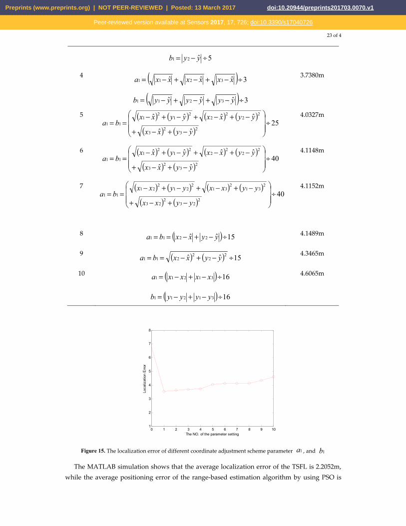
Hence, we survey the effect of the coordinate adjustment parameter settings on the localization error. We discuss lots of cases, and here we just list ten of them which the localization error is relatively small. We list the parameter settings of 1a and 1b , and the NO (#) of the cases, the different localization errors in Table 2. The coordinate of the UN is ),,( zyx , the coordinate of LN1 is ),,( 111 zyx , the coordinate of LN2 is ),,( 222 zyx , the coordinate of LN3 is ),,( 333 zyx , and the coordinate of EN is )ˆ,ˆ,ˆ( zyx . Note LN2 corresponding to the point that

the angle is the largest angle in the triangle. We use the No (#). of the cases is 0 to express CRFLA. Then we discuss many cases of the parameter settings and choose ten of them to show the localization error. We can see the different parameter settings can decrease the localization error at different extent. Compared with the localization error of CRFLA, the localization error of all the cases is reduced and show it in Figure 15.

Table 2. The parameter setting of the coordinate adjustment scheme and their own localization error

No (#) The parameter setting of the 1a and 1b Average localization error

0 011 == ba 6.7996m

1 xxa ˆ21 −=

yyb ˆ21 −=

3.5348m

2 2ˆ21 +−= xxa

1ˆ21 +−= yyb

3.6220m

3 5ˆ21 ÷−= xxa 3.6815m

0 20 40 60 80 100 120-2

0

2

4

6

8

10

12

14

16

Sensor Nodes

Loca

lizat

ion

Err

or

Circle-based Range-free Localization Algorithm

The Extension of Circle-based Range-free Algorithm




http://dx.doi.org/10.3390/s17040726

23 of 4

5ˆ21 ÷−= yyb

4 ( ) 3ˆˆˆ 3211 ÷−+−+−= xxxxxxa

( ) 3ˆˆˆ 3211 ÷−+−+−= yyyyyyb

3.7380m

5 ( ) ( ) ( ) ( )( ) ( )

25ˆˆ

ˆˆˆˆ

23

23

22

22

21

21

11 ÷

−+−+

−+−+−+−==

yyxx

yyxxyyxxba

4.0327m

6 ( ) ( ) ( ) ( )( ) ( )

40ˆˆ

ˆˆˆˆ

23

23

22

22

21

21

11 ÷

−+−+

−+−+−+−==

yyxx

yyxxyyxxba

4.1148m

7 ( ) ( ) ( ) ( )( ) ( )

402

232

23

231

231

221

221

11 ÷

−+−+

−+−+−+−==

yyxx

yyxxyyxxba

4.1152m

8 ( ) 15ˆˆ 2211 ÷−+−== yyxxba 4.1489m

9 ( ) ( ) 15ˆˆ 22

2211 ÷−+−== yyxxba

4.3465m

10 ( ) 1631211 ÷−+−= xxxxa

( ) 1631211 ÷−+−= yyyyb

4.6065m

Figure 15. The localization error of different coordinate adjustment scheme parameter 1a , and 1b

The MATLAB simulation shows that the average localization error of the TSFL is 2.2052m, while the average positioning error of the range-based estimation algorithm by using PSO is

0 1 2 3 4 5 6 7 8 9 101

2

3

4

5

6

7

8

The NO. of the parameter setting

Loca

lizat

ion

Err

or




http://dx.doi.org/10.3390/s17040726

24 of 4

0.8985m. The PSO algorithm can efficiently improve the localization error of the TSFL algorithm. In Phase II, we use CRFLA to locate the unlocalized sensor nodes, and the localization ratio achieved is 96.38% while the localization ratio of using TSFL is 82.13%. The average localization error of CRFLA is 6.7996m while using the coordinate adjustment scheme the average localization error can decrease to 3.5348m.

9. Conclusions

To make better use of underwater resources and realize the application of UWSNs, the localization of sensor nodes for UWSNs is the critical issue. Many scholars put forward different localization techniques of UWSNs. However, most of them are based on the assumption of accurate synchronization between sensor nodes. In fact, it is tough to achieve. TP-TSFLA in this paper contains two phase, namely, range-based estimation phase and range-free evaluation phase. The PSO algorithm can decrease the localization error for TSFL. CRFLA locates the unlocalized sensor nodes. We use the multi-stage scheme that the localized sensor nodes are looked like the new anchor nodes to help realize localization. Besides, a coordinate adjustment scheme is extended to improve the precision of circle-based range-free algorithm. The simulation results show that TP-TSFLA can achieve a relative localization ratio without time synchronization and the PSO algorithm and the coordinate adjustment scheme can decrease the localization error. However, there are still some issues to study. We design the two conditions based on the experience and experiment. Therefore it just can only guarantee with a high probability the selected anchor nodes is optimal. We will further improve the two conditions. If the coordinate adjustment scheme is designed more reasonable, the localization error will decrease a lot. Hence, we will find the better parameter setting of the coordinate adjustment scheme. The impact of the localization protocols on the routing and clustering protocols is also a direction in the future.

Acknowledgments: This work was supported in part by the Overseas Academic Training Funds,

University of Electronic Science and Technology of China (OATF, UESTC) (Grant no. 201506075013), and the

Program for Science and Technology Support in Sichuan Province (Grant nos. 2014GZ0100 and 2016GZ0088).

Author Contributions: JHL and LYF conceived and designed the experiments; LYF performed the experiments; JHL and LYF analyzed the data; JHL contributed reagents/materials/analysis tools; LYF wrote the paper.

Conflicts of Interest: The authors declare no conflict of interest.

References

1. R. Kumar; and N. Singh. A survey on data aggregation and clustering schemes in underwater sensor networks. International Journal of Grid and Distributed Computing 2014; Volume. 7, pp. 29-52.

2. E. Felemban; F.K. Shaikh; U.M. Qureshi; A.A. Sheikh; S.B. Qaisar. Underwater sensor network applications: a comprehensive survey. International Journal of Distributed Sensor Networks, 2015; Volume. 2015, pp. 1-14.

3. L. Tetley; D. Calcutt. Electronic navigation systems, 3rd ed.; Routledge, Taylor and Francis Group, London and New York, 2001.




http://dx.doi.org/10.3390/s17040726

25 of 4

4. E. Kaushal; G. Kaddoum. Underwater optical wireless communication, IEEE Access 2016; Volume. 4, pp.1518 - 1547.

5. J. Heidemann; W. Ye; J. Wills; A. Syed; Y. Li. Research challenges and applications for underwater sensor networking, in Proceedings of the IEEE Wireless Communications and Networking Conference (WCNC ’06), pp. 228–235, April 2006.

6. M. Erol-Kantarci; H.T. Mouftah; S. Oktug. A survey of architectures and localization techniques for underwater acoustic sensor networks. IEEE Communications Surveys & Tutorials 2011; Volume. 13, pp. 487-502.

7. H. Li; Y.H. He; X.Z. Cheng; H.S. Zhu; L.M. Sun. Security and privacy in localization for underwater sensor networks. IEEE Communications Magazine 2015; Volume. 53, pp. 56-62.

8. Y.J. Ren; N. Yu; L.R. Zhang; X. Wang; J.W. Wan. Set-membership localization algorithm based on adaptive error bounds for large-scale underwater wireless sensor networks. Electronics Letters 2013; Volume. 49, pp. 159-161.

9. B. Allotta; F. Bartolini; A. Caiti; et al. Typhoon at commsNet13: experimental experience on AUV navigation and localization. Annual Reviews in Control 2015; Volume. 40, pp. 157-171.

10. M. Beniwal; R. Singhn; A. Sangwan. A localization scheme for underwater sensor networks Without Time Synchronization. Wireless Pers Commun 2016; Volume. 88, pp. 537-55.

11. M. Erol-Kantarci; H. T. Mouftah; S. Oktug. A Survey of Architectures and Localization Techniques for Underwater Acoustic Sensor Networks. IEEE Communications Surveys & Tutorials 2011; Volume. 13, pp. 487-502.

12. Q. Fengzhong; W. Shiyuan; W. Zhihui; L. Zubin. A survey of ranging algorithms and localization schemes in an underwater acoustic sensor network. China Communications 2016; Volume. 13, pp. 66-81.

13. G. Han, J. Jiang; L. Shu; Y. Xu, F. Wang. Localization Algorithms of Underwater Wireless Sensor Networks: A Survey. Sensors 2012; Volume. 12, pp.2026-2061.

14. K. Nageswararao; U.D.Prasan. A Survey on Underwater Sensor Networks Localization Techniques. Academia Edu, 2013.

15. G Isbitiren; O.B Akan. Three-dimensional underwater target tracking with acoustic sensor networks. IEEE Transactions on Vehicular Technology 2011; Volume. 60, pp: 3897-3906.

16. M. Waldmeyer; H.P. Tan; W.K.G. Seah. Multi-stage AUV-aided Localization for Underwater Wireless Sensor Networks. 2011 IEEE Workshops of International Conference on Advanced Information Networking and Applications, Biopolis, 2011, pp. 908-913.

17. M. Moradi. A reverse localization scheme for underwater acoustic sensor networks. http://eprints.utm.my/33759/1 /MarjanMoradiMFSKSM2013ABS.pdf

18. M. Moradi; J. Rezazadeh; A.S. Ismail. A Reverse Localization Scheme for underwater acoustic sensor networks. Sensors 2012; Volume. 12, 2012, pp. 4352-4380.

19. L.F. Liu; J. G Wu; Z.W. Zhu. Multihops fitting approach for node localization in underwater wireless sensor networks. International Journal of Distributed Sensor Networks 2015; Volume. 2015, pp. 1-11.

20. C.R. Krishna; P.S. Yadav. A hybrid localization scheme for underwater wireless sensor networks. 2014 International Conference on Issues and Challenges in Intelligent Computing Techniques (ICICT) 2014.

21. Y. Guo; Y.T. Liu. Localization for anchor-free underwater sensor networks. Computers & Electrical Engineering 2013; Volume. 39, pp. 1812-1821.




http://dx.doi.org/10.3390/s17040726

26 of 4

22. M. Waldmeyer; H.P. Tan; W.K.G. Seah. Multi-stage AUV-aided localization for underwater wireless sensor networks. Advanced Information Networking and Applications (WAINA) 2011; 2011 IEEE Workshops of International Conference on, Biopolis, pp. 908-913.

23. V. Chandrasekhar; W. Seah. An area localization scheme for underwater sensor networks. OCEANS 2006 - Asia Pacific, Singapore, 2006, pp. 1-8.

24. S. Zhu; N. Jin; L. Wang; X. Zheng; S. Yang; M. Zhu. A novel dual-hydrophone localization method in underwater sensor networks. 2016 IEEE/OES China Ocean Acoustics (COA), Harbin, 2016, pp. 1-4.

25. R. Zandi; M. Kamerei; H. Amini; F. Yaghoubi. Underwater sensor network positioning using an AUV Moving on a Random Waypoint Path. IETE Journal of Research 2015; Volume. 61, pp. 693-698.

26. R. Zandi; M. Kamerei; H. Amini. Distributed estimation of sensors position in an underwater wireless sensor network. International Journal of Electronics 2015; pp. 1-15.

27. W. Cheng; A. Thaeler; X. Cheng; F. Liu; X. Lu; Z. Lu. Time-synchronization-free localization in large scale underwater acoustic sensor networks.Distributed Computing Systems Workshops, 2009. ICDCS Workshops '09. 29th IEEE International Conference on, Montreal, QC, 2009, pp. 80-87.

28. P.T.V. Bhuvaneswari; S. Karthikeyan; B. Jeeva; M.A. Prasath. An Efficient Mobility Based Localization in Underwater Sensor Networks.2012 Fourth International Conference on Computational Intelligence and Communication Networks, Mathura, 2012, pp. 90-94.

29. R. Zhao; X. Shen; J. Gao; Y. Zhang; H. Wang. Localization in underwater acoustic networks based on double rates. 2012 Oceans, Hampton Roads, VA, 2012, pp. 1-4.

30. R. Diamant; L. Lampe. Underwater Localization with Time-Synchronization and Propagation Speed Uncertainties. IEEE Transactions on Mobile Computing 2013; Volume. 12, pp. 1257-1269.

31. Z. Zhou; Z. Peng; J. H. Cui; Z. Shi; A. Bagtzoglou. Scalable Localization with Mobility Prediction for Underwater Sensor Networks. IEEE Transactions on Mobile Computing 2011; Volume. 10, pp. 335-348.

32. A. Kurniawan; H.W. Ferng. Projection-based localization for underwater sensor networks with consideration of layers. IEEE 2013 Tencon - spring, Sydney, NSW, 2013, pp. 425-429.

33. Y. Ren; N. Yu; X. Guo; J. Wan. Cube-scan-based three dimensional localization for large-scale Underwater Wireless Sensor Networks. 2012 IEEE International Systems Conference SysCon 2012, Vancouver, BC, 2012, pp. 1-6.

34. H.P. Tan; R. Diamant; W.K.G. Seah; M. Waldmeyer. A survey of techniques and challenges in underwater localization. Ocean Engineering 2011; Volume. 38, pp. 1663-1676.

35. T. Bian; R. Venkatesan; C. Li. Design and evaluation of a new localization scheme for underwater acoustic sensor networks. Global Telecommunications Conference, 2009. GLOBECOM 2009. IEEE, Honolulu, HI, 2009, pp. 1-5.

36. S.L. Zhang; Q. Zhang; M.Q. Liu; Z. Fan. A top-down positioning scheme for underwater wireless sensor networks. Science China Information Sciences 2013; Volume. 57, pp. 1-10.

© 2017 by the authors. Licensee Preprints, Basel, Switzerland. This article is an open access article distributed under the terms and conditions of the Creative Commons by Attribution (CC-BY) license (http://creativecommons.org/licenses/by/4.0/).




http://dx.doi.org/10.3390/s17040726

Documents

Two-Phase Time Synchronization-Free Localization Algorithm