Embed Size (px)
Citation preview

Diss. ETH No. 16106
Time Synchronization and Localizationin Sensor Networks
A dissertation submitted to theSwiss Federal Institute of Technology Zurich (ETH Zurich)
for the degree ofDr. sc. ETH Zurich
presented byKay Romer
Diplom-Informatiker, University of Frankfurt/Main, Germanyborn June 16, 1972citizen of Germany
accepted on the recommendation ofProf. Dr. Friedemann Mattern, examinerProf. Dr. Paul J. M. Havinga, co-examiner
2005

Abstract
So-called sensor nodes combine means for sensing environmental parameters, pro-cessors, wireless communication capabilities, and autonomous power supply in asingle compact device. Networks of these untethered devices can be deployedunobtrusively in the physical environment in order to monitor a wide variety ofreal-world phenomena with unprecedented quality and scale while only marginallydisturbing the observed physical processes.
Due to the close integration of sensor networks with the real world, the cate-gories time and location are fundamental for many applications of sensor networks,for example to interpret sensing results (e.g., where and when did an event occur)or for coordination among sensor nodes (e.g., which nodes can when be switchedto idle mode). Hence, time synchronization and sensor node localization are fun-damental and closely related services in sensor networks.
Existing solutions for these two basic services have been based on a rathernarrow notion of a sensor network as a large-scale, ad hoc, multi-hop, unpartitionednetwork of largely homogeneous, tiny, resource-constrained, mostly immobile sensornodes that would be randomly deployed in the area of interest. However, recentlydeveloped prototypical applications indicate that this narrow definition does notcover a significant portion of the application domain of wireless sensor networks.
Our thesis is that applications of sensor networks span a whole design spacewith many important dimensions. Existing solutions for time synchronization andnode localization do not cover important parts of this design space. Substantiallydifferent approaches are required to support these regions adequately. Such solutionscan actually be provided.
We support this thesis by proposing a design space of wireless sensor networkswhere concrete applications can be located at different points of the space. Weidentify two important regions in the design space that are not appropriately sup-ported by existing methods for time synchronization and node localization. Wealso propose, implement, and evaluate new solutions that cover these regions. Thepractical feasibility of our approaches is demonstrated by means of a typical sensornetwork application which requires time synchronization and node localization.
Our approach to time synchronization supports applications where networkconnectivity is intermittent. The idea underlying our Time-Stamp Synchronizationmethod is to avoid proactive synchronization of the clocks of all nodes in a network.Instead, the clocks of the sensor nodes run unsynchronized, each defining its ownlocal time scale. Only if clock readings are exchanged among nodes as time stamps
i

ii
contained in network messages, these time stamps are transformed from the timescale of the sender to the time scale of the receiver. This approach is scalable, sincetime is only synchronized on demand where and when needed by the application.The approach is also resource efficient, since it piggybacks on existing messageexchanges.
Our approach to node localization supports tiny sensor nodes known as SmartDust. The Lighthouse Location System is based on a single beacon device thatemits particular optical signal patterns. Sensor nodes can autonomously infer theirlocation by passively observing these signals. This approach is scalable, since eachnode infers its location independent of other nodes. A single beacon device emitslong-range signals in broadcast mode and can support arbitrary network densities.The approach is resource efficient, since the sensor nodes do not actively emit anysignals. Only a tiny, energy-efficient optical receiver is needed to infer locations.

Zusammenfassung
Sensoren zur Erfassung von Umweltparametern, Prozessoren, drahtlose Kommu-nikationseinheiten sowie autarke Energiequellen sind in sogenannten Sensorknotenauf kleinstem Raum integriert. Netze aus vielen solchen Knoten konnen unauf-dringlich in die Alltagswelt ausgebracht werden, um eine Reihe verschiedener Um-weltphanomene grossrauming und mit hoher Genauigkeit zu erfassen, ohne diebeobachteten Vorgange wesentlich zu beeinflussen.
Aufgrund der Einbettung von Sensornetzen in die reale Welt spielen die Katego-rien Raum und Zeit eine fundamentale Rolle fur viele Anwendungen, beispielsweisezur Interpretation von Beobachtungen (z.B. wo und wann wurde ein Ereignis fest-gestellt) oder fur die Koordination der Sensorknoten untereinander (z.B. welcheKnoten konnen wann in einen energiesparenden Schlafzustand geschaltet werden).Daher sind Zeitsynchronisation und Lokalisierung von Sensorknoten grundlegendeund eng verwandte Dienste in Sensornetzen.
Bestehende Ansatze zur Realisierung dieser Dienste gehen von einer vergleichs-weise engen Definition eines Sensornetzes aus, derzufolge ein Sensornetz aus ei-ner sehr grossen Zahl von homogenen, winzigen und daher ressourcenbeschranktenKnoten besteht, die vorwiegend immobil sind, nachdem sie zufallig im Zielge-biet verteilt wurden. Ferner geht man davon aus, das Sensornetze unpartitionierteMulti-Hop-Ad-Hoc-Netze sind. In jungerer Zeit wurde jedoch eine Vielzahl proto-typischer Anwendungen von Sensornetzen vorgestellt, denen eine solche enge Defi-nition nicht gerecht wird.
Unsere These ist daher, dass Applikationen von Sensornetzen einen umfangrei-chen Entwurfsraum aufspannen, der eine Vielzahl wichtiger Dimensionen umfasst.Bisher existierende Methoden zur Zeitsynchronisation und Lokalisierung deckenwichtige Bereiche dieses Entwurfsraums nicht ab. Vielmehr benotigt man neuarti-ge Herangehensweisen, um diese Bereiche adaquat zu unterstutzen. EntsprechendeTechniken konnen tatsachlich bereitgestellt werden.
Wir untermauern diese These, indem wir den Entwurfsraum von Sensornetzenexplizit machen und zeigen, dass konkrete Applikationen tatsachlich verschiede-nen Punkten in diesem Raum zugeordnet werden konnen. Wir identifizieren zweispezifische Bereiche im Entwurfsraum, welche nicht hinreichend durch bestehendeAnsatze zur Zeitsynchronisation und Lokalisierung unterstutzt werden. Um dieseBereiche abzudecken, schlagen wir neue Losungsansatze vor, zeigen prototypischeRealisierungen auf und evaluieren diese. Die praktische Umsetzbarkeit dieser Me-thoden zeigen wir anhand einer konkreten Applikation, die Synchronisation und
iii

iv
Lokalisierung voraussetzt.Unser Ansatz zur Zeitsynchronisation unterstutzt Anwendungsszenarien, in de-
nen Netzverbindungen nur sporadisch bestehen. Die grundlegende Idee fur dasVerfahren der Zeitstempelsynchronisation besteht darin, die Uhren der Sensorkno-ten nicht zu synchronisieren, so dass die lokale Uhr eines jeden Knotens eine un-abhangige Zeitskala definiert. Zeitstempel, die durch Auslesen der lokalen Uhr ent-stehen, haben daher zunachst nur lokale Gultigkeit. Wird ein solcher Zeitstempeljedoch als Teil einer Nachricht im Netz verschickt, so wird dabei der Zeitstempelvon der Zeitskala des Senders in die Zeitskala des Empfangers transformiert. DieserAnsatz ist skalierbar, da Synchronisation nur dann stattfindet, wenn sie tatsachlichvon der Applikation benotigt wird. Ferner kann diese Methode effizient implemen-tiert werden, da die fur die Zeitstempeltransformation notwendige Kommunikationin vielen Fallen Huckepack auf bereits existierenden Nachrichten realisiert werdenkann.
Unser Ansatz zur Lokalisierung unterstutzt winzige, sehr ressourcenarme Sen-sorknoten, die unter dem Namen “Smart Dust” bekannt sind. Unser Verfahren mitdem Namen Leuchtturmlokalisierung verwendet eine spezielle Basisstation, die spe-zifische optische Signale aussendet. Sensorknoten konnen allein durch passive Be-obachtung dieser Signale autonom ihre Position mit hoher Genauigkeit bestimmen.Dieser Ansatz ist skalierbar, da jeder Knoten vollig unabhangig von anderen Kno-ten seine Position bestimmt. Eine einzige Basistation kann daher beliebig dichtenNetzen zur Lokalisierung dienen. Da die Sensorknoten fur die Lokalisierung selbstkeinerlei Signale aussenden mussen, ist das Verfahren auf der Seite der Sensorkno-ten sehr ressourceneffizient. Sensorknoten benotigen nur einen einfachen optischenEmpfanger, der auf kleinstem Raum realisiert werden kann.

Contents
1 Introduction 11.1 Motivation . . . . . . . . . . . . . . . . . . . . . . . . . . . . . . . . 11.2 Contributions . . . . . . . . . . . . . . . . . . . . . . . . . . . . . . 31.3 Structure . . . . . . . . . . . . . . . . . . . . . . . . . . . . . . . . 3
2 Wireless Sensor Networks 52.1 Characterization . . . . . . . . . . . . . . . . . . . . . . . . . . . . 6
2.1.1 Distributed Systems . . . . . . . . . . . . . . . . . . . . . . 72.1.2 Ubiquitous Computing . . . . . . . . . . . . . . . . . . . . . 82.1.3 Peer-to-Peer Systems . . . . . . . . . . . . . . . . . . . . . . 92.1.4 Embedded Systems . . . . . . . . . . . . . . . . . . . . . . . 92.1.5 Remote and Wired Sensing . . . . . . . . . . . . . . . . . . 102.1.6 Wireless, Mobile, and Ad Hoc Networks . . . . . . . . . . . 112.1.7 Digital Signal Processing . . . . . . . . . . . . . . . . . . . . 11
2.2 The Sensor Network Design Space . . . . . . . . . . . . . . . . . . . 122.2.1 Deployment . . . . . . . . . . . . . . . . . . . . . . . . . . . 132.2.2 Mobility . . . . . . . . . . . . . . . . . . . . . . . . . . . . . 132.2.3 Cost, Size, Resources, and Energy . . . . . . . . . . . . . . . 132.2.4 Heterogeneity . . . . . . . . . . . . . . . . . . . . . . . . . . 142.2.5 Communication Modality . . . . . . . . . . . . . . . . . . . 142.2.6 Infrastructure . . . . . . . . . . . . . . . . . . . . . . . . . . 152.2.7 Network Topology . . . . . . . . . . . . . . . . . . . . . . . 162.2.8 Coverage . . . . . . . . . . . . . . . . . . . . . . . . . . . . . 162.2.9 Connectivity . . . . . . . . . . . . . . . . . . . . . . . . . . . 162.2.10 Network Size . . . . . . . . . . . . . . . . . . . . . . . . . . 172.2.11 Lifetime . . . . . . . . . . . . . . . . . . . . . . . . . . . . . 172.2.12 Other QoS Requirements . . . . . . . . . . . . . . . . . . . . 17
2.3 Implications of the Design Space . . . . . . . . . . . . . . . . . . . . 172.4 Applications . . . . . . . . . . . . . . . . . . . . . . . . . . . . . . . 18
2.4.1 Species Monitoring . . . . . . . . . . . . . . . . . . . . . . . 192.4.2 Environmental Monitoring . . . . . . . . . . . . . . . . . . . 212.4.3 Agriculture . . . . . . . . . . . . . . . . . . . . . . . . . . . 232.4.4 Production and Delivery . . . . . . . . . . . . . . . . . . . . 252.4.5 Disaster Relief . . . . . . . . . . . . . . . . . . . . . . . . . . 26
v

CONTENTS vi
2.4.6 Building Management and Automation . . . . . . . . . . . . 272.4.7 Traffic and Infrastructure . . . . . . . . . . . . . . . . . . . 282.4.8 Home and Office . . . . . . . . . . . . . . . . . . . . . . . . 292.4.9 Military and Homeland Security . . . . . . . . . . . . . . . . 302.4.10 Surveillance and Law Enforcement . . . . . . . . . . . . . . 322.4.11 Health Care . . . . . . . . . . . . . . . . . . . . . . . . . . . 33
2.5 Sensor Node Prototypes . . . . . . . . . . . . . . . . . . . . . . . . 342.5.1 Motes . . . . . . . . . . . . . . . . . . . . . . . . . . . . . . 342.5.2 Egrains . . . . . . . . . . . . . . . . . . . . . . . . . . . . . 362.5.3 Smart Dust . . . . . . . . . . . . . . . . . . . . . . . . . . . 372.5.4 Commodity Devices . . . . . . . . . . . . . . . . . . . . . . 39
2.6 Technical Challenges . . . . . . . . . . . . . . . . . . . . . . . . . . 392.6.1 Resource and Energy Constraints . . . . . . . . . . . . . . . 392.6.2 Network Dynamics . . . . . . . . . . . . . . . . . . . . . . . 402.6.3 Network Size and Density . . . . . . . . . . . . . . . . . . . 422.6.4 Unattended and Untethered Operation . . . . . . . . . . . . 42
2.7 Design Principles . . . . . . . . . . . . . . . . . . . . . . . . . . . . 422.7.1 Adaptive Tradeoffs . . . . . . . . . . . . . . . . . . . . . . . 422.7.2 Multi-Modality . . . . . . . . . . . . . . . . . . . . . . . . . 432.7.3 Local Interaction . . . . . . . . . . . . . . . . . . . . . . . . 432.7.4 Data Centricity . . . . . . . . . . . . . . . . . . . . . . . . . 432.7.5 In-Network Data Processing . . . . . . . . . . . . . . . . . . 442.7.6 Cross-Layer Interaction . . . . . . . . . . . . . . . . . . . . . 44
2.8 Summary . . . . . . . . . . . . . . . . . . . . . . . . . . . . . . . . 44
3 Space and Time in Sensor Networks 463.1 Uses of Space and Time . . . . . . . . . . . . . . . . . . . . . . . . 46
3.1.1 Sensor Network – Observer . . . . . . . . . . . . . . . . . . . 473.1.2 Sensor Network – Real World . . . . . . . . . . . . . . . . . 473.1.3 Within a Sensor Network . . . . . . . . . . . . . . . . . . . . 48
3.2 Locating Nodes in Spacetime . . . . . . . . . . . . . . . . . . . . . 493.2.1 Internal vs. External . . . . . . . . . . . . . . . . . . . . . . 503.2.2 Global vs. Local . . . . . . . . . . . . . . . . . . . . . . . . 513.2.3 Point Estimates vs. Bounds . . . . . . . . . . . . . . . . . . 523.2.4 Points vs. Distances . . . . . . . . . . . . . . . . . . . . . . 533.2.5 Scope and Lifetime . . . . . . . . . . . . . . . . . . . . . . . 533.2.6 Precision . . . . . . . . . . . . . . . . . . . . . . . . . . . . . 543.2.7 Other Quality-of-Service Aspects . . . . . . . . . . . . . . . 54
3.3 Distributed Algorithms for Localization in Spacetime . . . . . . . . 553.3.1 Bootstrapping . . . . . . . . . . . . . . . . . . . . . . . . . . 573.3.2 Obtaining Constraints . . . . . . . . . . . . . . . . . . . . . 583.3.3 Combining Constraints . . . . . . . . . . . . . . . . . . . . . 583.3.4 Selecting Constraints . . . . . . . . . . . . . . . . . . . . . . 593.3.5 Maintaining Localization over Time . . . . . . . . . . . . . . 60
CONTENTS vii
3.4 Limitations and Trade-offs . . . . . . . . . . . . . . . . . . . . . . . 613.4.1 Anchor Infrastructure . . . . . . . . . . . . . . . . . . . . . 613.4.2 Energy and Other Resources . . . . . . . . . . . . . . . . . . 633.4.3 Network Dynamics . . . . . . . . . . . . . . . . . . . . . . . 643.4.4 Configuration . . . . . . . . . . . . . . . . . . . . . . . . . . 64
3.5 Summary . . . . . . . . . . . . . . . . . . . . . . . . . . . . . . . . 65
4 Time Synchronization 664.1 Background . . . . . . . . . . . . . . . . . . . . . . . . . . . . . . . 66
4.1.1 Clock and Communication Models . . . . . . . . . . . . . . 664.1.2 Obtaining Constraints . . . . . . . . . . . . . . . . . . . . . 684.1.3 Combining Constraints . . . . . . . . . . . . . . . . . . . . . 704.1.4 Maintaining Synchronization . . . . . . . . . . . . . . . . . . 714.1.5 Selecting Constraints . . . . . . . . . . . . . . . . . . . . . . 73
4.2 Related Work . . . . . . . . . . . . . . . . . . . . . . . . . . . . . . 744.2.1 Logical Time . . . . . . . . . . . . . . . . . . . . . . . . . . 744.2.2 Offline Time Synchronization . . . . . . . . . . . . . . . . . 744.2.3 Network Time Protocol (NTP) . . . . . . . . . . . . . . . . 754.2.4 Time Synchronization for Sensor Networks . . . . . . . . . . 76
4.3 Problem Statement . . . . . . . . . . . . . . . . . . . . . . . . . . . 814.3.1 Intermittent Connectivity . . . . . . . . . . . . . . . . . . . 814.3.2 Resource Efficiency . . . . . . . . . . . . . . . . . . . . . . . 824.3.3 Precision for Collocated Nodes . . . . . . . . . . . . . . . . . 824.3.4 Correctness . . . . . . . . . . . . . . . . . . . . . . . . . . . 82
4.4 Time-Stamp Synchronization . . . . . . . . . . . . . . . . . . . . . 824.4.1 Algorithm Overview . . . . . . . . . . . . . . . . . . . . . . 834.4.2 Assumptions . . . . . . . . . . . . . . . . . . . . . . . . . . . 844.4.3 Time Transformation . . . . . . . . . . . . . . . . . . . . . . 844.4.4 Message Delay Estimation . . . . . . . . . . . . . . . . . . . 854.4.5 Time-Stamp Calculation . . . . . . . . . . . . . . . . . . . . 864.4.6 Interval Arithmetic . . . . . . . . . . . . . . . . . . . . . . . 884.4.7 Implementation . . . . . . . . . . . . . . . . . . . . . . . . . 894.4.8 Evaluation . . . . . . . . . . . . . . . . . . . . . . . . . . . . 924.4.9 Potential Improvements . . . . . . . . . . . . . . . . . . . . 94
4.5 Summary . . . . . . . . . . . . . . . . . . . . . . . . . . . . . . . . 96
5 Sensor Node Localization 975.1 Background . . . . . . . . . . . . . . . . . . . . . . . . . . . . . . . 97
5.1.1 Signal Propagation and Mobility Models . . . . . . . . . . . 975.1.2 Obtaining Constraints . . . . . . . . . . . . . . . . . . . . . 1005.1.3 Combining Constraints . . . . . . . . . . . . . . . . . . . . . 1025.1.4 Maintaining Localization . . . . . . . . . . . . . . . . . . . . 1055.1.5 Selecting Constraints . . . . . . . . . . . . . . . . . . . . . . 106
5.2 Related Work . . . . . . . . . . . . . . . . . . . . . . . . . . . . . . 1075.2.1 Traditional Localization Approaches . . . . . . . . . . . . . 107

CONTENTS viii
5.2.2 Centralized Localization for Sensor Networks . . . . . . . . . 1085.2.3 Distributed Localization for Sensor Networks . . . . . . . . . 110
5.3 Problem Statement . . . . . . . . . . . . . . . . . . . . . . . . . . . 1145.3.1 Device Challenges . . . . . . . . . . . . . . . . . . . . . . . . 1145.3.2 Resource Efficiency . . . . . . . . . . . . . . . . . . . . . . . 1145.3.3 Minimal Infrastructure . . . . . . . . . . . . . . . . . . . . . 1155.3.4 Scalability . . . . . . . . . . . . . . . . . . . . . . . . . . . . 115
5.4 The Lighthouse Location System . . . . . . . . . . . . . . . . . . . 1155.4.1 An Idealistic System . . . . . . . . . . . . . . . . . . . . . . 1155.4.2 A Realistic System . . . . . . . . . . . . . . . . . . . . . . . 1185.4.3 Prototype Implementation . . . . . . . . . . . . . . . . . . . 1255.4.4 Evaluation . . . . . . . . . . . . . . . . . . . . . . . . . . . . 129
5.5 Summary . . . . . . . . . . . . . . . . . . . . . . . . . . . . . . . . 137
6 Application Experience 1386.1 Object Tracking with Smart Dust . . . . . . . . . . . . . . . . . . . 1386.2 Object Detection . . . . . . . . . . . . . . . . . . . . . . . . . . . . 1396.3 Data Fusion . . . . . . . . . . . . . . . . . . . . . . . . . . . . . . . 1416.4 Node Localization . . . . . . . . . . . . . . . . . . . . . . . . . . . . 1426.5 Time Synchronization . . . . . . . . . . . . . . . . . . . . . . . . . 1436.6 Message Ordering . . . . . . . . . . . . . . . . . . . . . . . . . . . . 1436.7 Evaluation . . . . . . . . . . . . . . . . . . . . . . . . . . . . . . . . 1446.8 Discussion . . . . . . . . . . . . . . . . . . . . . . . . . . . . . . . . 1466.9 Summary . . . . . . . . . . . . . . . . . . . . . . . . . . . . . . . . 147
7 Conclusions and Future Work 1487.1 Contributions . . . . . . . . . . . . . . . . . . . . . . . . . . . . . . 1487.2 Limitations . . . . . . . . . . . . . . . . . . . . . . . . . . . . . . . 149
7.2.1 Time-Stamp Synchronization . . . . . . . . . . . . . . . . . 1497.2.2 Lighthouse Location System . . . . . . . . . . . . . . . . . . 149
7.3 Future Work . . . . . . . . . . . . . . . . . . . . . . . . . . . . . . . 1507.3.1 Time-Stamp Synchronization . . . . . . . . . . . . . . . . . 1507.3.2 Lighthouse Location System . . . . . . . . . . . . . . . . . . 1507.3.3 Service Interfaces . . . . . . . . . . . . . . . . . . . . . . . . 1517.3.4 Service Selection and Adaptation . . . . . . . . . . . . . . . 1517.3.5 Calibration . . . . . . . . . . . . . . . . . . . . . . . . . . . 152
7.4 Concluding Remarks . . . . . . . . . . . . . . . . . . . . . . . . . . 152

Chapter 1
Introduction
Enabled by technological advancements in wireless communications and embeddedcomputing, wireless sensor networks were first considered for military applicationsin the 1980-ies, where large-scale wireless networks of autonomous sensor nodeswould enable the unobtrusive observation of events in the real-world. Since then,the use of sensor networks has also been considered for various civil applicationdomains. This thesis is devoted to two fundamental services required by sensornetworks: time synchronization and node localization.
In this inaugural chapter, we introduce the research area of wireless sensornetworks, motivate the need for time synchronization and localization in sensornetworks, and give a brief overview of the main contributions of our work. Weconclude this chapter with an overview of the remainder of this thesis.
1.1 Motivation
In the late 1980-ies, technology advanced to a stage where it became possible tobuild relatively small, battery-powered computing devices equipped with sensorsand wireless communication with manageable effort and cost by leveraging off-the-shelf hardware components. While systems with similar functionality had beenbuilt earlier, these required costly custom hardware design processes or exhibited apower consumption that did not allow battery operation for longer periods of time.
Having observed the speed of technological advancements over the past, onecould envision at that time that in the near future it would be possible to build evensmaller untethered computing, communicating, and sensing devices with marginalcost per device. While the low per-device cost would allow mass production, smallsize and untetheredness would enable an unobtrusive deployment.
This prospect triggered researchers to think of implications and applications ofthis emerging new technology. Perhaps one of the first individuals to articulate thistrend, to envision possible applications, and to speculate about societal impactswas Mark Weiser, who coined the term Ubiquitous Computing in his seminal article[106]. From then on, this vision was further refined and substantiated by a numberof visionaries and research projects. This development was evidenced by several
1

CHAPTER 1. INTRODUCTION 2
new terms such as Pervasive Computing, Ambient Intelligence, and also WirelessSensor Networks (WSN).
Common to these slightly different terms and underlying visions is the goal ofbridging the long-standing gap between the physical world where we live in and thetraditional virtual world of computers and other information-technology artifacts.The key to realization of these visions is the use of large collections of these unobtru-sive networked computers that could perceive and control aspects of the real worldvia sensors and actuators on the one hand, and that would provide an intuitive in-terface to human users on the other hand. While projects classified as UbiquitousComputing, Pervasive Computing, and Ambient Intelligence are somewhat focusedon issues related to interfacing these unobtrusive networked computing devices tohuman users, this component is of lesser significance in projects that examine sen-sor networks. Rather, research on wireless sensor networks focuses on the technicalaspects of observing the real world with best possible quality, using as few as pos-sible resources, and minimizing the impact of the observation tool on the observedphysical processes. We examine the subtle differences of the above research areasin more detail in Chapter 2. Our work, however, is focused on wireless sensornetworks.
WSN have been initially considered for military applications, where real-worldevents (e.g., vehicles and troops passing) must be unobtrusively observed in inac-cessible or hostile environments. For example, DARPA initiated the DistributedSensor Networks program in the 1980-ies. For these military tasks, large numbersof sensor nodes would be deployed in the area of interest and form a wireless net-work to observe events in the physical environment. These long-lived, unattendednetworks would be unobtrusive due to the small size and untetheredness of indi-vidual nodes, could operate without the use of additional hardware infrastructure,and would be robust due to the redundant deployment of nodes. Later on, it wassuggested that these features would render sensor networks a useful tool also ina number of civil application domains [35], for example as a scientific tool for en-vironmental monitoring or in building automation. In Chapter 2 we examine anumber of concrete civil applications of WSN.
Time and space are fundamental categories in the physical world. Since wirelesssensor networks are a tool for observing, influencing, and reasoning about phenom-ena of the physical word, time and space are also of utmost importance in WSN.They are essential elements for obtaining and interpreting real-world observations(e.g., where and when did an event occur, how large and fast was an observedobject), for tasking a sensor network (e.g., where and when to look for events), forinterfacing wireless sensor networks with the real-world (e.g., what node densityand sampling frequency is needed to observe a certain object), and for coordinationamong sensor nodes (e.g., which nodes can when be switched to idle mode).
There are two basic services to enable these functions: time synchronizationand localization of sensor nodes. Time synchronization allows a sensor node toestimate current time with respect to a common time scale. Localization allows anode to estimate its current location with respect to a common coordinate system.

CHAPTER 1. INTRODUCTION 3
1.2 Contributions
This thesis is devoted to time synchronization and node localization in the contextof wireless sensor networks. What makes the provision of these services challeng-ing are the specific technical characteristics and requirements of wireless sensornetworks and their applications. A number of earlier research projects and com-monly used hardware prototypes of sensor nodes led to a rather narrow view onthese characteristics and requirements, which resulted in a de facto definition of awireless sensor network that is adopted by most research projects. Consequently,existing work on time synchronization and node localization is mostly based onthis narrow view.
One of the contributions of this thesis is to show that such a narrow viewon the characteristics and requirements of WSN does not meet the diversity ofconcrete applications of wireless sensor networks. Motivated by a study of concreteapplications of WSN, we propose to replace this narrow definition with a multi-dimensional design space that captures influential and significant dimensions ofwireless sensor networks and their applications. We substantiate the relevance ofsuch a design space by showing that concrete prototypical applications of wirelesssensor networks can indeed be located at a diverse set of points in the design space.
We show that existing approaches to time synchronization and node localizationfail to cover important parts of this design space. In particular, we identify tworegions in the design space which are not sufficiently supported by existing solu-tions. The main contribution of this thesis is to propose novel approaches to nodelocalization and time synchronization to support these regions. We present andevaluate prototypical implementations of our solutions. In addition, we supportthe practical feasibility of our algorithms by incorporating them into a concreteapplication for tracking mobile objects with a wireless sensor network.
One further contribution of this thesis is the provision of a unified view on timesynchronization and node localization in the context of wireless sensor networks.While research in these two domains has been largely separated in the past, weshow that models, requirements, techniques, and algorithms of the two domainsare rather similar and in some respects closely related. In particular, we pointout a number of structural elements that are shared by many existing distributedalgorithms for time synchronization and node localization.
The major contributions of this thesis have also been published in scientificconferences, journals, and books, most notably in [34, 80, 82, 83, 84, 85, 86].
1.3 Structure
This thesis first discusses general aspects of wireless sensor networks, before pre-senting a unified framework for the discussion of time and space. Based on thisframework, we discuss time synchronization and node localization separately. Wethen rejoin our discussion on time and space by showing how our solutions are

CHAPTER 1. INTRODUCTION 4
employed in a common prototypical application. In more detail, the thesis is struc-tured as follows:
Chapter 2 is devoted to general aspects of wireless sensor networks. We char-acterize wireless sensor networks by showing how they draw from other researchdomains and point out important differences with respect to these domains. Wethen propose the design space of wireless sensor networks and justify it by showingthat existing applications do indeed cover different regions in this space. We dis-cuss different classes of sensor-node prototypes and show how they cover variousregions of the design space. We then discuss how different regions in the designspace are associated with different technical challenges and conclude the chapterwith design principles that are helpful in dealing with these challenges.
Chapter 3 presents a unified framework for the discussion of aspects related tospace and time in sensor networks. We first present applications of space and timein sensor networks, before developing a common model for time synchronizationand node localization. Based on this common model, we present requirementsand possible conceptual approaches for time synchronization and node localization.Then we examine the structure of distributed algorithms for time synchronizationand node localization, pointing out five important structural elements that canbe found in most distributed algorithms of both domains. Finally, we discussvarious limitations and trade-offs of these distributed algorithms with respect tothe technical challenges presented in Chapter 2.
Chapters 4 and 5 are devoted to in-detail examinations of time synchronizationand node localization, respectively. The structure of these two chapters is verysimilar. Following the framework developed in Chapter 3, we first review funda-mental concepts and techniques. Based on these concepts, we present and discussconcrete existing algorithms. We then show how these approaches fail to meet therequirements of certain important regions in the design space that was developed inChapter 2. Finally, we present and evaluate our solutions for these specific regionsin the design space.
In Chapter 6 we show the practical feasibility of our solutions for time synchro-nization and node localization by means of a concrete prototypical application.
Chapter 7 concludes this thesis by summarizing the results, by discussing limi-tations, and by providing an outlook on future work.

Chapter 2
Wireless Sensor Networks
Research on wireless sensor networks goes back to a number of US-based researchprojects, where the use of large networks of tiny wireless sensor devices was ex-plored in a military domain. Initial work mainly focused on the development ofhardware prototypes and energy-efficient networking protocols. These early ef-forts established a de facto definition of a wireless sensor network as a large-scale,wireless, ad hoc, multi-hop, unpartitioned network of homogeneous, tiny, mostlyimmobile sensor nodes that would be randomly deployed in the area of interest.
Since then, the use of wireless sensor networks has also been considered fora number of civil applications. Wireless sensor networks have been suggested asa scientific tool for better understanding real-world phenomena, as an enablingtechnology for making our daily life more comfortable, as a tool for improving theefficiency of industrial processes, and as a mechanism for dealing with issues suchas environmental protection and law enforcement. In these application domains,wireless sensor networks are deemed a promising technology with the potential forchanging the way we live by bridging the gap between the real world and the virtualworld of existing information technology.
The diverse set of potential applications has two important implications.Firstly, wireless sensor networks cannot any longer be characterized by a single,narrow definition. Rather, wireless sensor networks span a broad design space withvastly varying requirements and characteristics. Secondly, wireless sensor networkshave become a truly multidisciplinary domain, where close cooperation betweenusers, application domain experts, hardware designers, and software developers isneeded to realize efficient systems for specific applications.
In this chapter, we characterize wireless sensor networks in a number of dif-ferent ways. We first informally define wireless sensor networks in Section 2.1,also pointing out the research areas that are influential. In Section 2.2 we makethe design space of wireless sensor networks explicit by identifying its importantdimensions. We consider existing and envisioned applications of wireless sensornetworks in Section 2.4 and show that these applications do indeed cover variousregions in the design space. In Section 2.5 we discuss four classes of sensor nodeprototypes and show how these can cover different areas in the design space. Sec-
5

CHAPTER 2. WIRELESS SENSOR NETWORKS 6
tion 2.6 is devoted to prominent technical challenges that can be found at differentpoints in the design space. Design principles that can help mitigate these technicalchallenges are presented in Section 2.7.
2.1 Characterization
Sensor networks consist of sensor nodes – untethered computing devices that in-clude a power source, a transceiver for wireless communication, a processor, mem-ory, sensors, and potentially also actuators. Although the exact properties andcapabilities of these components may vary, a common property of sensor nodes istheir resource scarcity.
Multiple sensor nodes form a wireless network, whose topology and other prop-erties do also depend on the application context. A large class of sensor networkscan be characterized as multi-hop ad hoc networks, where sensor nodes do not onlyact as data sources, but also as routers that forward messages on behalf of othernodes, such that no additional communication infrastructure (e.g., base stations)is required for operating the network.
The sensor nodes participating in a network can vary in their capabilities andconfiguration. For example, sensor nodes may be equipped with different types ofsensors; some sensor nodes might be equipped with a more powerful processor andmore memory to perform sophisticated computations; some nodes might be con-nected to a other networks and can act as gateways to a background infrastructure.
Wireless sensor networks are deployed in the physical environment in order tomonitor a wide variety of real-world phenomena with unprecedented quality andscale (by placing many sensor nodes close to the phenomenon of interest), while onlymarginally disturbing the observed physical processes (due to the unobtrusivenessof individual sensor nodes).
Using attached sensors, nodes can observe a partial state of the real worldin their close physical neighborhood. By integrating observations of many sensornodes, a more detailed and geographically extensive observation of a partial stateof the real world can be obtained. Due to the relatively small effective range ofsensor nodes, sensor networks often consist of many, densely deployed sensor nodes.
While individual sensor nodes have only limited functionality, the global be-havior of a sensor network can be quite complex. The true value of the network isin this emergent behavior: the functionality of the whole is greater than the sumof its parts. For example, a sensor network may estimate the velocity of a movingobject even though sensor nodes are not equipped with velocity sensors. Instead,velocity estimates can be obtained by correlating object sightings from spatiallydispersed sensor nodes, which requires only sensors for detecting the proximity ofobjects.
The output of the sensor network may be used for various purposes. In themost basic form, the output is delivered to a human user for further evaluation.However, the output may also be used to control the operation of the sensor net-work without human intervention by enabling/disabling sensors, or by controlling
CHAPTER 2. WIRELESS SENSOR NETWORKS 7
operation parameters of sensors (e.g., sampling rate, sensitivity, orientation, posi-tion). In addition, actuators may be triggered based on the output of the sensornetwork. Using the output of the sensor network to control sensors or actuators caneffectively create a closed-loop system that strives to achieve a particular nominalcondition in the sensor network or in the real world.
Sensor networks are a multidisciplinary area of research which is related toand draws from a number of other research domains. However, due to a numberof novel characteristics and requirements of sensor networks, results from otherresearch domains typically cannot be directly applied to sensor networks. Belowwe further characterize wireless sensor networks by discussing closely related andinfluential research domains. In particular, we point out how sensor networks differfrom typical assumptions and models in these domains.
2.1.1 Distributed Systems
According to [7], a distributed system is an information-processing system thatcontains a number of independent computers that cooperate with one another overa communications networks in order to achieve a specific objective. Based onthis definition, wireless sensor networks are clearly distributed systems: sensornodes nodes cooperate by means of wireless communication in order to processinformation about the real world.
In the sensor network context, computers and communications network differsignificantly from many traditional distributed systems. The unobtrusive deploy-ment of large-scale sensor networks requires that sensor nodes be untethered, small,and cheap. Size and cost constraints in turn imply that sensor nodes are limitedin their resources (computing, storage, communication) and energy budget. Com-munication is wireless, typically short range, low bandwidth, and unreliable. In-teraction with a harsh physical environment may lead to a high degree of networkdynamics (e.g., topology changes, network partitions, node failures, communicationfailures) typically not found in traditional distributed systems.
Traditional distributed systems are mostly decoupled from the real world. Incontrast, sensor networks are inherently and closely integrated with the real world,with data about the physical environment being captured and processed automat-ically, online, and in real time. The input of a sensor network can be characterizedas a continuous stream of data with low information density (raw sensory data con-tains few information per bit), with high data volume (since many nodes frequentlysample their sensors), with many redundancies and correlations (since many phys-ical phenomena are continuous in time and space), and with a high level of noise(since data is obtained by measurements using low-cost sensors). The desiredoutput typically has opposite characteristics: high information density, low datevolume, low redundancy, and high accuracy.
Sensor nodes cooperate with the goal of distilling the essence of informationcontained in a large amount of dispersed sensor readings, taking into account thelimitations of individual nodes and the limitations of the communications network.

CHAPTER 2. WIRELESS SENSOR NETWORKS 8
2.1.2 Ubiquitous Computing
The term “Ubiquitous Computing” [106] refers to a world where computers areunobtrusively integrated into our natural environment in order to support us in-tuitively in fulfilling our tasks. This vision is based on the observation that usingtoday’s general purpose computers often requires complex and non-intuitive in-teraction patterns. Humans have to pay special attention to the computer, aredistracted from the task to be solved – ultimately making the computer a very vis-ible component of our current world. In contrast, using a “ubiquitous computer”should not require abilities that are not immediately related to the task at hand.In addition to this smooth integration into our natural environment, ubiquitouscomputers are also physically embedded into our environment and interact withthe physical world by means of sensors and actuators.
One possible way to approach this vision is to integrate computing andinformation-processing capabilities into familiar artifacts or into our physical envi-ronment – resulting in so-called “smart things” and “smart environments”. Here,the term “smart” refers to an augmented functionality that is both intuitive anduseful. In contrast to traditional general purpose computers, smart things andenvironments are highly specialized for a particular application. The comput-ers embedded into smart things and smart environments communicate with eachother or with a background infrastructure via a wireless network in order to providecomplex services.
Important for the intuitive or smart behavior of ubiquitous computing systemsis the notion of context. According to [29], context is any information that charac-terizes the situation of an entity (e.g., person, place, object). While this is a verybroad characterization, context information (e.g., location, time, light, tempera-ture, presence/absence of other entities) can often be circumscribed as the state ofan entity and its close physical environment. In most cases, sensors are used to ac-quire context information. Context is a key to intuitive usage, since it is a primarysource of information for adapting system behavior to the current situation andexpectations of users. In the ubicomp literature, such context-driven adaptation isreferred to as “context awareness”.
From the above description, wireless networks of embedded sensing and com-puting devices are a key enabling technology for ubicomp and have been used inmany prototypical ubicomp applications to date. Despite this, it is interesting tonote that the ubicomp and WSN research communities are largely separated bothin terms of research groups and venues for presenting research results.
One reason for this might be the somewhat different research foci of the twocommunities. Typical topics in ubicomp research are user-interface issues, applica-tions and their implications, high-level aspects of context acquisition and contextawareness. The WSN community often focuses on networking aspects, distributedalgorithms, and distributed signal processing. One further difference is related tothe use of networked sensors in ubicomp and WSN. Sensors for context acquisitionin ubicomp are often incorporated into specific artifacts, resulting in a predefinedand fixed association of sensors to a particular artifact. Detecting the context of

CHAPTER 2. WIRELESS SENSOR NETWORKS 9
such instrumented entities typically involves only a single or few networked sensors.Deriving context information from raw sensor readings is often performed outsideof the “sensor network”.
In contrast, typical wireless sensor networks are embedded into the environmentto monitor phenomena occurring within this environment. Often, these phenomenacannot be directly instrumented with sensors for observation. As a consequence,there may be no predefined or fixed association of sensor nodes to a monitoredphenomenon. Also, a large number of sensor nodes may be involved in the obser-vation of a single phenomenon. A changing set of sensor nodes may be involved inmonitoring a single phenomenon over time. Raw sensor readings are often (pre-)processed inside the sensor network.
Despite these subtle differences, the transition between ubicomp and WSN israther smooth, which will also be reflected by the design space we propose later inthis chapter.
2.1.3 Peer-to-Peer Systems
Peer-to-peer (P2P) systems can be defined as self-organizing, decentralized dis-tributed systems where nodes have symmetric roles. While originally conceivedfor file sharing in the Internet, the scalability and resilience of P2P systems lendsitself to a growing domain of applications. Most P2P research is concerned withthe establishment of so-called overlay networks on top of existing communicationinfrastructures such as the Internet. Such techniques effectively shield applicationdesigners from the complexities of organizing and maintaining an overlay topology,of tolerating node failures, of balancing load, and of locating application objects.
P2P systems share a number of properties with wireless sensor networks, namelythey are both large-scale, self-organizing, decentralized distributed systems. Hence,there is a high potential for P2P techniques in the sensor network context. However,there are also a number of differences between typical P2P systems and WSN,which make an adoption non-trivial. Most prominently, P2P systems are typicallydesigned for wired networks, where nodes do not suffer from resource and energyconstraints. Also, neighbor nodes in overlay networks often map to distant nodesin the underlying physical network. In the sensor network context, this may resultin poor performance and high energy consumption.
2.1.4 Embedded Systems
Many artifacts of our daily life such as consumer electronics, other consumer prod-ucts, and vehicles contain computers, which are commonly referred to as embeddedsystems. These embedded computing systems monitor and control certain aspectsof the containing system. In contrast to general purpose computing systems, em-bedded system perform a single or tightly knit set of application-specific functions,are often subject to real-time constraints, and must meet stringent dependabilityrequirements.

CHAPTER 2. WIRELESS SENSOR NETWORKS 10
Embedded computing systems show a high level of diversity, ranging from cen-tralized, highly cost/resource/energy-constrained systems (e.g., a pocket remotecontrol), to high-performance distributed embedded systems (e.g., an aircraft au-topilot). Most distributed embedded systems use wired communication, because itis less prone to communication errors and offers more deterministic behavior thanwireless communication.
An embedded system consists of hardware and software components, wherethe allocation of functions to hardware and software is highly dependent on therequirements of the actual system. For performance and security reasons, partof the functionality may be provided by application-specific hardware components.The use of software in conjunction with programmable hardware provides flexibilityand support for more complex features.
What differentiates wireless sensor networks from traditional embedded systemsis the large number of participating nodes, the use of wireless communication,and often severe resource/cost/energy constraints of sensor nodes. Traditionalembedded systems are typically a fixed part of highly engineered structures, thatis, the actual “embedding” takes place at production time and does not changeduring the lifetime of the embedded system. In contrast, wireless sensor nodes maybe deployed in a natural setting with little control over the actual placement anddistribution of the nodes. Also, the embedding (i.e., deployment) of sensor nodesinto the physical environment is not tied to the production time of the sensor nodeand may change during the lifetime of a sensor node.
2.1.5 Remote and Wired Sensing
Many existing systems for observing real-world phenomena are based on few sen-sors with a relatively long range, such as satellites for earth observation, weatherstations, or sonars. Due to the long range, these systems can observe phenomenathat are far away from the sensors. However, the resolution of these systems de-creases with the observation distance. Moreover, many systems require a free lineof sight between the sensors and the observed phenomenon.
Wireless sensor nodes are equipped with short range sensors. Many of thesedevices are placed in the close vicinity of the observed phenomenon. Since theaverage distance between the observed phenomenon and the sensors is small andsince many redundant sensors observe a single phenomenon, the effective monitor-ing resolution of a wireless sensor network can be better than that of a remotesensing approach. The placement of the sensors close the phenomenon allows theuse of wireless sensor networks also in cluttered environments where line-of-sightpaths are rather short.
Many existing systems make use of distributed, wired sensors that are connectedto a central computing device (e.g., sensors in cars and engines, sonar arrays).Such an approach has a number of advantages: sensors do not need separate powersupplies, the wired network has a fixed topology, small and deterministic delays,communication errors are very rare. On the other hand, the wiring limits theflexibility and scale of such wired sensor networks.

CHAPTER 2. WIRELESS SENSOR NETWORKS 11
2.1.6 Wireless, Mobile, and Ad Hoc Networks
Wireless communication, especially with focus on short communication range andlow power consumption, is a key enabling technology for wireless sensor networks.In mobile networks, computers capable of wireless communication can change theirphysical position over time, resulting in dynamically changing network topologies.Ad hoc networks are wireless networks that do not require an external infrastructuresuch as base stations in mobile phone networks. The nodes of an ad hoc networkact both as sources/sinks of messages and as routers that forward messages onbehalf of other nodes. Nodes can join and leave the network anytime. Althoughad hoc networks may also consist of immobile nodes, they often contain mobilenodes. Power awareness is an important issue in the context of mobile networks,since mobile computing devices are often powered by batteries. Recent research inmobile ad hoc networks focuses on routing, mobility management, power manage-ment, self-configuration, and the radio interface (including the radio hardware andmedium access techniques).
It is anticipated that many wireless sensor networks will be implemented as amobile ad hoc network (MANET). However, results from MANET research oftencannot be directly applied to wireless sensor networks, since resource and energyconstraints are typically more stringent here. Typical MANET research focuseson handheld devices or laptops with renewable batteries. The computing, storage,communication resources of these devices are comparable to desktop computers.In contrast, sensor node batteries are often not replaceable; range, bandwidth,reliability of wireless communication links, computing and memory resources, andavailable energy may be orders of magnitude smaller compared to more traditionalMANET nodes.
Wireless sensor networks may also rely on infrastructure-based mobile networks.For example, mobile phone companies are currently exploring the value of mobilephones for sensor networks. Such networks could either solely consist of mobilephones equipped with sensors, or a mobile phone could act as a gateway con-necting an ad hoc sensor network to the phone network. Such combinations ofinfrastructure-based and ad hoc networks would allow remote access to sensor net-works and an integration with existing computing infrastructures.
2.1.7 Digital Signal Processing
Digital signal processing (DSP) can be defined as the analysis and modification ofdiscrete time signals (i.e., sequences of numbers). It is a key technology for systemsthat process signals from the real world. While wireless sensor networks do processreal-world signals, there are quite a number of differences between many traditionalsignal processing systems and sensor networks.
First of all, many traditional DSP application are centralized, that is, data frompossibly many sources is collected at a single processor for evaluation. Dependingon the bandwidth of the input signals, this approach may require high-bandwidthcommunication channels and a very powerful centralized processor.
CHAPTER 2. WIRELESS SENSOR NETWORKS 12
In typical sensor networks, the effective channel bandwidth and processingpower is typically rather limited. Hence, centralized processing of digital signalsis often not desirable. Rather, input signals should be preprocessed locally onthe originating sensor nodes to extract relevant features that can be communi-cated more efficiently. Hence, DSP in sensor networks is often decentralized anddistributed over the sensor nodes.
2.2 The Sensor Network Design Space
In the recent past, wireless sensor networks have found their way into a wide varietyof applications and systems with vastly varying requirements and characteristics.As a consequence, it is becoming increasingly difficult to discuss typical require-ments regarding hardware issues and software support. This is particularly prob-lematic in a multidisciplinary research area such as wireless sensor networks, whereclose collaboration between users, application domain experts, hardware designers,and software developers is needed to implement efficient systems.
Initial research into wireless sensor networks was mainly motivated by militaryapplications, with DARPA continuing to fund a number of prominent researchprojects (e.g., Smart Dust, NEST) that are commonly regarded as the cradle ofsensor-network research. The type of applications considered by these projectsled to a de facto definition of a wireless sensor network as a large-scale (possiblythousands of nodes, covering large geographical areas), wireless, ad hoc, multi-hop,unpartitioned network of homogeneous, tiny (hardly noticeable), mostly immobile(after deployment) sensor nodes that would be randomly deployed in the area ofinterest.
More recently, other, civilian application domains of wireless sensor networkshave been considered, such as environmental and species monitoring, agriculture,production and delivery, healthcare, etc. (see Section 2.4). Concrete projectstargeting these application areas indicate that the above definition of a wirelesssensor network does not necessarily apply for these applications – networks mayconsist of heterogeneous and mobile sensor nodes, the network topology may beas simple as a star topology, networks may make use of existing communicationinfrastructures, etc. To meet this general trend towards diversification, we willdiscuss important dimensions of the sensor network design space in the followingsubsections. We will informally characterize each of the dimensions and, whereappropriate, identify (possibly orthogonal) property classes in order to support acoarse-grained classification of sensor network applications.
It is certainly debatable which issues are important enough to be explicitlyconsidered as dimensions in the design space and one could argue in favor of addingmore dimensions or removing some from our suggestions detailed below. In fact,we expect that this might become reasonable in the future as the field and itsapplications evolve. However, we have tried to ensure that our initial suggestionconsisted of a sensible set of dimensions, by basing our choice on the following twoprinciples. Firstly, there should be notable variability between applications with

CHAPTER 2. WIRELESS SENSOR NETWORKS 13
respect to dimensions. Secondly, a dimension should have a significant impact onthe design and implementation of technical solutions.
In the subsequent section we show that existing and envisioned applicationsof wireless sensor networks can indeed be located at different points in the designspace, with a number of important implications.
2.2.1 Deployment
The deployment of sensor nodes in the physical environment may take severalforms. Nodes may be deployed at random (e.g., by dropping them from an aircraft)or installed at deliberately chosen spots. Deployment may be a one-time activity,where the installation and use of a sensor network are strictly separate activities.However, deployment may also be a continuous process, with more nodes beingdeployed at any time during the use of the network – for example, to replace failednodes or to improve coverage at certain interesting locations.
The actual type of deployment affects important properties such as the expectednode density, node locations, regular patterns in node locations, and the expecteddegree of network dynamics.
We suggest the following coarse-grained classification with respect to deploy-ment: random vs. manual; one-time vs. iterative.
2.2.2 Mobility
Sensor nodes may change their location after initial deployment. Mobility canresult from environmental influences such as wind or water, sensor nodes may beattached to or carried by mobile entities, and sensor nodes may possess automotivecapabilities. In other words, mobility may be either an incidental side effect, orit may be a desired property of the system (e.g., to move nodes to interestingphysical locations), in which case mobility may be either active (i.e., automotive)or passive (e.g., attached to a moving object not under the control of the sensornode). Mobility may apply to all nodes within a network or only to subsets ofnodes. The degree of mobility may also vary from occasional movement with longperiods of immobility in between, to constant travel.
Mobility has a large impact on the expected degree of network dynamics andhence influences the design of networking protocols and distributed algorithms. Theactual speed of movement may also have an impact, for example on the amount oftime during which nodes stay within communication range of each other.
We suggest the following coarse-grained classification with respect to mobility:immobile vs. partly vs. all; occasional vs. continuous; active vs. passive.
2.2.3 Cost, Size, Resources, and Energy
Depending on the actual needs of the application, the form factor of a single sensornode may vary from the size of a shoe box (e.g., a weather station) to a microscop-ically small particle (e.g., for military applications where sensor nodes should be

CHAPTER 2. WIRELESS SENSOR NETWORKS 14
almost invisible). Similarly, the cost of a single device may vary from hundreds ofEuros (for networks of very few, but powerful nodes) to a few Cents (for large-scalenetworks made up of very simple nodes).
Since sensor nodes are untethered autonomous devices, their energy and otherresources are limited by size and cost constraints. Varying size and cost constraintsdirectly result in corresponding varying limits on the energy available (i.e., size,cost, and energy density of batteries or devices for energy scavenging), as well ason computing, storage, and communication resources. Hence, the energy and otherresources available on a sensor node may also vary greatly from system to system.Power may be either stored (e.g., in batteries) or scavenged from the environment(e.g., by solar cells).
These resource constraints limit the complexity of the software executed onsensor nodes. For our classification, we have partitioned sensor nodes roughly intofour classes based on their physical size: brick vs. matchbox vs. grain vs. dust.
2.2.4 Heterogeneity
Early sensor network visions anticipated that sensor networks would typically con-sist of homogeneous devices that were mostly identical from a hardware and soft-ware point of view. Some projects, such as Amorphous Computing [1], even as-sumed that sensor nodes were indistinguishable, that is, they did not even possessunique addresses or IDs within their hardware. This view was based on the obser-vation that otherwise it would not be feasible to cheaply produce vast quantitiesof sensor nodes.
However, in many prototypical systems available today, sensor networks consistof a variety of different devices. Nodes may differ in the type and number of at-tached sensors; some computationally more powerful “compute” nodes may collect,process, and route sensory data from many more limited sensing nodes; some sen-sor nodes may be equipped with special hardware such as a GPS receiver to act asbeacons for other nodes to infer their location; some nodes may act as gateways tolong-range data communication networks (e.g., GSM networks, satellite networks,or the Internet).
The degree of heterogeneity in a sensor network is an important factor since itaffects the complexity of the software executed on the sensor nodes and also themanagement of the whole system.
We suggest the following coarse-grained classification with respect to hetero-geneity: homogeneous vs. heterogeneous.
2.2.5 Communication Modality
For wireless communication among sensor nodes, a number of communicationmodalities can be used such as radio, diffuse light, laser, inductive and capaci-tive coupling, or even sound.
The most common modality is radio waves, since these do not require a free
CHAPTER 2. WIRELESS SENSOR NETWORKS 15
line of sight, and communication over medium ranges can be implemented withrelatively low power consumption and relatively small antennas (a few centimetersin the common sub-GHz frequency bands). Using light beams for communicationrequires a free line of sight and may interfere with ambient light and daylight, butallows for much smaller and more energy-efficient transceivers compared to radiocommunication. Smart Dust [49], for example, uses laser beams for communication.Inductive and capacitive coupling only works over small distances, but may beused to power a sensor node. Most passive Radio Frequency Identification (RFID)systems use inductive coupling, for example. Sound or ultrasound is typically usedfor communication under water or to estimate distances based on time-of-flightmeasurements. Sometimes, multiple modalities are used by a single sensor networksystem.
The communication modality used obviously influences the design of mediumaccess protocols and communication protocols, but also affects other propertiesthat are relevant to the application.
We suggest the following coarse-grained classification with respect to commu-nication modality: radio vs. light vs. inductive vs. capacitive vs. sound.
2.2.6 Infrastructure
The various communication modalities can be used in different ways to construct anactual communication network. Two common forms are so-called infrastructure-based networks on the one hand and ad hoc networks on the other hand. Ininfrastructure-based networks, sensor nodes can only directly communicate withso-called base station devices. Communication between sensor nodes is relayedvia the base station. If there are multiple base stations, these have to be ableto communicate with each other. The number of base stations depends on thecommunication range and the area covered by the sensor nodes. Mobile phonenetworks and Smart Dust [49] are examples of this type of network.
In ad hoc networks, nodes can directly communicate with each other withoutan infrastructure. Nodes may act as routers, forwarding messages over multiplehops on behalf of other nodes.
Since the deployment of an infrastructure is a costly process, and the installationof an infrastructure may often not be feasible, ad hoc networks are preferred formany applications. However, if an infrastructure is already available anyway (suchas the GSM network), it might also be used for certain sensor network applications.
Combinations of ad hoc networks and infrastructure-based networks are some-times used, where clusters of sensor nodes are interconnected by a wide areainfrastructure-based network.
Note that the above arguments not only apply to communication, but alsoto other infrastructures, such as localization or time synchronization (e.g., GPSsatellites).
We suggest the following coarse-grained classification with respect to infrastruc-ture: infrastructure vs. ad hoc.
CHAPTER 2. WIRELESS SENSOR NETWORKS 16
2.2.7 Network Topology
One important property of a sensor network is its diameter, that is, the maximumnumber of hops between any two nodes in the network. In its simplest form, asensor network forms a single-hop network, with every sensor node being able todirectly communicate with every other node. An infrastructure-based network witha single base station forms a star network with a diameter of two. A multi-hopnetwork may form an arbitrary graph, but often an overlay network with a simplerstructure is constructed such as a tree or a set of connected stars.
The topology affects many network characteristics such as latency, robustness,and capacity. The complexity of data routing and processing also depends on thetopology.
We suggest the following coarse-grained classification with respect to networktopology: single-hop vs. star vs. networked stars vs. tree vs. graph.
2.2.8 Coverage
The effective range of the sensors attached to a sensor node defines the coveragearea of a sensor node. Network coverage measures the degree of coverage of thearea of interest by sensor nodes. With sparse coverage, only parts of the area ofinterest are covered by the sensor nodes. With dense coverage, the area of interestis completely (or almost completely) covered by sensors. With redundant coverage,multiple sensors cover the same physical location. The actual degree of coverage ismainly determined by the observation accuracy and redundancy required. Coveragemay vary across the network. For example, nodes may be deployed more denselyat interesting physical locations.
The degree of coverage also influences information-processing algorithms. Highcoverage is a key to robust systems and may be exploited to extend the networklifetime by switching redundant nodes to power-saving sleep modes.
We suggest the following coarse-grained classification with respect to coverage:sparse vs. dense vs. redundant.
2.2.9 Connectivity
The communication ranges and physical locations of individual sensor nodes definethe connectivity of a network. If there is always a network connection (possiblyover multiple hops) between any two nodes, the network is said to be connected.Connectivity is intermittent if the network may be occasionally partitioned. Ifnodes are isolated most of the time and enter the communication range of othernodes only occasionally, we say that communication is sporadic. Note that despitethe existence of partitions, messages may be transported across partitions by mobilenodes.
Connectivity mainly influences the design of communication protocols andmethods of data gathering.

CHAPTER 2. WIRELESS SENSOR NETWORKS 17
We suggest the following coarse-grained classification with respect to connec-tivity: connected vs. intermittent vs. sporadic.
2.2.10 Network Size
The number of nodes participating in a sensor network is mainly determined byrequirements relating to network connectivity and coverage, and by the size of thearea of interest. The network size may vary from a few nodes to thousands of sensornodes or even more. The network size determines the scalability requirements withregard to protocols and algorithms.
2.2.11 Lifetime
Depending on the application, the required lifetime of a sensor network may rangefrom some hours to several years. The necessary lifetime has a high impact on therequired degree of energy efficiency and robustness of the nodes.
2.2.12 Other QoS Requirements
Depending on the application, a sensor network must support certain quality-of-service aspects such as real-time constraints (e.g., a physical event must bereported within a certain period of time), robustness (i.e., the network should re-main operational even if certain well-defined failures occur), tamper-resistance (i.e.,the network should remain operational even when subject to deliberate attacks),eavesdropping-resistance (i.e., external entities cannot eavesdrop on data traffic),unobtrusiveness or stealth (i.e., the presence of the network must be hard to de-tect). These requirements may impact on other dimensions of the design spacesuch as coverage and resources.
2.3 Implications of the Design Space
There are several important consequences of the design space as discussed above.Clearly, a single hardware platform will most likely not be sufficient to support thewide range of possible applications (cf. Section 2.5). In order to avoid the devel-opment of application-specific hardware, it would be desirable, however, to haveavailable a (small) set of platforms with different capabilities that cover the designspace. A modular approach, where the individual components of a sensor node canbe easily exchanged, might help to partially overcome this difficulty. Principles andtools for selecting suitable hardware components for particular applications wouldalso be desirable.
As similar observation can be made regarding algorithms and software in gen-eral. As with hardware, one could try to cover the design space with a (larger)set of different protocols, algorithms, and basic services. Note that this does inparticular apply to algorithms for locating sensor nodes in space and time as will
CHAPTER 2. WIRELESS SENSOR NETWORKS 18
be discussed in Chapter 3. The selection of appropriate software components forthe application at hand and perhaps also dynamic adaptation during runtime ofan application should be supported by appropriate frameworks.
In traditional distributed systems, middleware has been introduced to hidesuch complexity from the software developer by providing programming abstrac-tions that are applicable for a large class of applications. This raises the question,whether appropriate abstractions and middleware concepts can be devised that areapplicable for a large portion of the sensor network design space. This is not aneasy task, since some dimensions of the design space (e.g., network connectivity)are very hard to hide from the system developer. Moreover, exposing certain appli-cation characteristics to the system and vice versa is a key approach for achievingenergy and resource efficiency in sensor networks. Even if the provision of ab-straction layers is conceptually possible, they often introduce significant resourceoverheads – which is problematic in highly resource-constrained environments suchas sensor networks.
In addition to these more technical issues, the design space we advocate canhopefully bring more clarity to the often somewhat diffuse discussions about typicalor right characteristics and requirements of wireless sensor networks.
2.4 Applications
Wireless sensor networks can be considered as a tool for observing real-world pro-cesses. In particular, the use of WSN might be a worthwhile option for observationtasks with one or more of the following properties:
• The observation environment is cluttered and can be hardly observed fromafar.
• Any instrumentation for observation must be unobtrusive to avoid influencingobservation results.
• The phenomenon of interest or its close physical environment can be instru-mented for observation.
• A high spatial and temporal monitoring resolution is required.
• The signal-to-noise ratio of signals emitted by the phenomenon of interest islow or decreases significantly over distance.
• Traditional observation methods are very costly due to the involvement ofhuman personnel.
• The observation environment is very harsh, inaccessible, or even toxic.
• The observation must be continuously performed during long periods of timeor over large geographical areas.

CHAPTER 2. WIRELESS SENSOR NETWORKS 19
The above problem characterization applies to a wide range of problem domainssome of which we will sketch in the following sections. For each of these domainswe describe some representative applications. We also show that these applicationscan be located at different points in the design space. In addition to these concreteapplications, we briefly sketch application ideas and visions that have not yet beenrealized or which are not well-documented.
2.4.1 Species Monitoring
Wireless sensor networks can be used to observe the behavior of animals in theirnatural habitats. Cerpa et al [22] give an overview and motivation of this applica-tion domain.
Bird Observation at Great Duck Island
A WSN is being used to observe the breeding behavior of a small bird calledLeach’s Storm Petrel [58] on Great Duck Island, Maine, USA. These birds areeasily disturbed by the presence of humans, hence WSN seems an appropriateway of better understanding their behavior. The breeding season lasts for sevenmonths from April to October. The biologists are interested in the usage patternof their nesting burrows, changes in environmental conditions outside and insidethe burrows during the breeding season, variations among breeding sites, and theparameters of preferred breeding sites.
Sensor nodes are installed inside the burrows and on the surface. Nodes canmeasure humidity, pressure, temperature, and ambient light level. Burrow nodesare equipped with infrared sensors to detect the presence of the birds. The burrowsoccur in clusters and the sensor nodes form a multi-hop ad hoc network. Eachnetwork cluster contains a sensor node with a long-range directional antenna thatconnects the cluster to a central base station computer. The base station computeris connected to a database back-end system via a satellite link. Sensor nodes sampletheir sensors about once a minute and send their readings directly to the databaseback-end system.
Deployment manual, one-timeMobility immobileResources matchboxCost approx. 200 USD per nodeEnergy battery, solar panelHeterogeneity weather stations, burrow nodes, gatewaysModality radioInfrastructure base station, gatewaysTopology star of subgraphsCoverage dense (every burrow)Connectivity connected

CHAPTER 2. WIRELESS SENSOR NETWORKS 20
Size tens to hundreds (about 100 deployed)Lifetime 7 months (breeding period)
ZebraNet
A WSN is being used to observe the behavior of wild animals within a spacioushabitat (e.g., wild horses, zebras, and lions) [48] at the Mpala Research Center inKenya. Of particular interest is the behavior of individual animals (e.g., activitypatterns of grazing, graze-walking, and fast moving), interactions within a species,interactions among different species (e.g., grouping behavior and group structure),and the impact of human development on the species. The observation period isscheduled to last a year or more. The observation area may be as large as hundredsor even thousands of square kilometers.
Animals are equipped with sensor nodes. An integrated GPS receiver is usedto obtain estimates of their position and speed of movement. Light sensors areused to give an indication of the current environment. Further sensors (head up ordown, body temperature, ambient temperature) are planned for the future. Eachnode logs readings from its sensors every three minutes. Whenever a node entersthe communication range of another node, the sensor readings and the identitiesof the sensor nodes are exchanged (i.e., data is flooded across network partitions).At regular intervals, a mobile base station (e.g., a car or a plane) moves throughthe observation area and collects the recorded data from the animals it passes.
Deployment manual, one-timeMobility all, continuous, passiveResources matchboxEnergy batteryHeterogeneity nodes, gatewayModality radioInfrastructure base station, GPSTopology graphCoverage dense (every animal)Connectivity sporadicSize tens to hundredsLifetime one year
Further Applications in Species Monitoring
A variety of different sensor devices are used to monitor the behavior of WhaleSharks [137] around the Seychelles. The so-called archival pop-off tag is attachedto the shark and uses light and pressure sensors to monitor the diving behavior.After a certain time, the tag detaches from the shark and floats to the surface,from where it sends off collected data to a satellite.
Sensor devices are also used to observe social interactions among seals [127] in

CHAPTER 2. WIRELESS SENSOR NETWORKS 21
the Northern Sea. A sensor node [37] is attached to each seal which can detect thedistance to and the identity of another nearby tag (and seal). These sightings arecollected and sent off to a satellite.
A project at CENS intends to use a sensor network for detection and classi-fication of marine microorganisms (e.g., alga) that are toxic to marine life anddangerous to human health [123]. Work in this project has so far focused on thedevelopment of appropriate sensors. Obviously, these sensors cannot be attachedto microorganisms, but have to be installed in an area of interest in the ocean.
2.4.2 Environmental Monitoring
Besides animals, a number of other environmental phenomena can be observedwith wireless sensor networks.
Glacier Monitoring
A sensor network is being used to monitor sub-glacier environments at Briksdals-breen, Norway, with the overall goal of better understanding the Earth’s climate[62]. Of particular interest are displacements and the dynamics inside the glacier.A lengthy observation period of months to years is required.
Sensor nodes are deployed in drill holes at different depths in the glacier iceand in the till beneath the glacier. Sensor nodes are equipped with pressure andtemperature sensors and a tilt sensor for measuring the orientation of the node.Sensor nodes communicate with a base station deployed on top of the glacier.The base station measures supra-glacial displacements using differential GPS andtransmits the data collected via GSM. Nodes are not recoverable after deployment.Radio communication through ice and water is a major problem.
Deployment manual, one-timeMobility all, continuous, passiveResources brickEnergy batteryHeterogeneity nodes, base stationModality radio, GSMInfrastructure base station, GPS, GSMTopology starCoverage sparseConnectivity connectedSize 9 deployed (potential for tens to hundreds)Lifetime several months
Bathymetry
A sensor network is being used to monitor the impact on the surrounding environ-ment of a wind farm off the coast of England [61]. Of particular interest here is

CHAPTER 2. WIRELESS SENSOR NETWORKS 22
the influence on the structure of the ocean bed (e.g., formation of sand banks) andthe influence on tidal activity.
Sensor nodes are deployed on the ocean bed by dropping them from a shipat selected positions, their location being fixed on the ocean bed by an anchor.Each sensor node is connected via a cable to a buoy on the ocean surface thatcontains the radio equipment and GPS, since radio communication under water isvirtually impossible. The sensor nodes are able to measure pressure, temperature,conductivity, current, and turbidity, and form a self-organized ad hoc network.
Deployment manual, one-timeMobility all, occasional, passiveResources brickEnergy batteryHeterogeneity homogeneousModality radioInfrastructure GPSTopology graphCoverage sparse (500m - 1km apart)Connectivity connectedSize 6 deployed, 50 planned (potential for up to hundreds)Lifetime several months
Ocean Water Monitoring
The ARGO project [112] is using a sensor network to observe the temperature,salinity, and current profile of the upper ocean. The goal is a quantitative descrip-tion of the state of the upper ocean and the patterns of ocean climate variability,including heat and freshwater storage and transport. Intended coverage is global,and observation is planned to last for several years. Measurement data is availablealmost in real-time.
The project uses free-drifting profiling sensor nodes equipped with temperatureand salinity sensors. The nodes are dropped from ships or planes. The nodescycle to a depth of 2000m every ten days. Data collected during these cycles istransmitted to a satellite while nodes are at the surface. The lifetime of the nodesis about 4-5 years.
Deployment random, iterativeMobility all, continuous, passiveResources brickCost approx. 15000 USD per nodeEnergy batteryHeterogeneity homogeneousModality radioInfrastructure satellite

CHAPTER 2. WIRELESS SENSOR NETWORKS 23
Topology starCoverage sparseConnectivity intermittentSize 1300 deployed (3000 planned)Lifetime 4-5 years
Further Applications in Environmental Monitoring
Several projects explore the use of sensor networks for monitoring water quality.The European project SEWING [129] is currently concerned with the developmentof sensors for certain chemicals. It is, however, anticipated to construct completesensor nodes for water quality monitoring. At CENS, a similar project intends toobserve water quality and to monitor transport of contaminants with ground waterusing sensor networks [118].
In [107], as wireless sensor network for monitoring volcanic eruptions is pre-sented. The system consists of several infrasound monitoring nodes, which reportlow-frequency acoustic signals to an aggregator node, which preprocesses the dataand sends aggregated values to a remote base station via a long-range radio link.A GPS node is used to synchronize the infrasound monitoring nodes. The systemcan be used to monitor and locate volcanic eruptions.
Sensor networks can be used to monitor seismic activity and the structuralresponse of buildings [51]. A number of experiments with seismic sensor networksin buildings have been carried out within CENS [109, 128]. A sensor network isalso used to monitor the influence of winds on Golden Gate Bridge in San Francisco[133].
Another application of sensor networks is the observation of micro climates andtheir changes over time [27, 122]. One particularly interesting application in thiscontext is the use of sensor networks for detecting signs of life on other planets(e.g., on Mars) [28].
2.4.3 Agriculture
Wireless sensor networks can also be used to increase the efficiency of plant breedingand livestock husbandry.
Grape Monitoring
A WSN is being used to monitor the conditions that influence plant growth (e.g.,temperature, soil moisture, light, and humidity) across a large vineyard in Ore-gon, USA [11]. The goals include supporting precision harvesting (harvesting anarea as soon as the grapes in it are ripe), precision plant care (adapting the wa-ter/fertilizer/pesticide supply to the needs of individual plants), frost protection,predicting insect/pest/fungi development, and developing new agricultural models.

CHAPTER 2. WIRELESS SENSOR NETWORKS 24
In a first version of the system, sensor nodes are deployed across a vineyardin a regular grid about 20 meters apart. A temperature sensor is connected toeach sensor node via a cable in order to minimize false sensor readings due to heatdisseminated by the sensor nodes. A laptop computer is connected to the sensornetwork via a gateway to display and log the temperature distribution across thevineyard. The sensor nodes form a two-tier multi-hop network, with nodes in thesecond tier sending data to a node in the first tier. Nodes in the first tier alsocollect sensor data, but do additionally act as data routers.
Deployment manual, one-timeMobility immobileResources matchboxCost 200 USD per nodeEnergy batteryHeterogeneity sensors, gateway, base stationModality radioInfrastructure base stationTopology tree (two-tiered multi-hop)Coverage sparse (20m apart)Connectivity connectedSize 65 deployed (potential for up to hundreds)Lifetime several months (growth period)
Cattle Herding
A WSN is being used to implement virtual fences, with an acoustic stimulus beinggiven to animals that cross a virtual fence line [18]. Movement data from the cowscontrols the virtual fence algorithm that dynamically shifts fence lines. Such asystem can reduce the overheads of installing and moving physical fences and canimprove the usage of feedlots.
For the first experiment, each sensor node consists of a PDA with a GPS re-ceiver, a WLAN card, and a loudspeaker for providing acoustic stimuli to the cattleas they approach a fence. These devices are attached to the neck of the cows. Thenodes form a multi-hop ad hoc network, forwarding movement data to a base sta-tion (a laptop computer). The base station transmits fence coordinates to thenodes.
Deployment manual, one-timeMobility all, continuous, passiveResources brickCost approx. 1000 USD per nodeEnergy batteryHeterogeneity homogeneousModality radioInfrastructure base station, GPS

CHAPTER 2. WIRELESS SENSOR NETWORKS 25
Topology graphCoverage dense (every cow)Connectivity intermittentSize 10 deployed (potential for up to hundreds)Lifetime days to weeks
Further Applications in Agriculture
The Hogthrob project [135] intends to use sensor networks for sow monitoring. Inparticular, movement data is intended to be used to detect the sow’s heat periodand to detect abnormal behavior which could be caused by diseases.
The PlantCare project [53] uses a sensor network to monitor soil humidity ofplants and to control a robot to water indigent plants.
2.4.4 Production and Delivery
In this section we consider the use of wireless sensor networks for monitoring theproduction and delivery of goods.
Cold Chain Management
The commercial Securifood system [78] is a WSN for monitoring the temperaturecompliance of cold chains from production, via distribution centers and stores, tothe consumer. Clients receive an early warning of possible breaks in the cold chain.
The system consists of four major components: sensor nodes, relay units, accessboxes, and a warehouse. Sensor nodes are transported with the products and collecttemperature data. Relay units collect and store temperature data from sensor nodes– they are more powerful devices with a permanent power supply. Multiple relayunits form a multi-hop ad hoc network. An access box is an even more powerfulembedded Linux device that acts as a gateway between the network of relay unitsand the Internet. There is one access box per production site. An Internet-hosteddata warehouse acts as a central server, collecting data from all the access boxes.The data warehouse provides an online image of all the sensor data in the systemand acts as a central data repository for applications.
Deployment manual, iterativeMobility partly (sensors), occasional, passiveResources matchbox (sensors), brick (relays)Energy batteryHeterogeneity sensor units, relay units, access boxes, warehouseModality radioInfrastructure relays, access boxesTopology tree (three-tiered multi-hop)Coverage sparse

CHAPTER 2. WIRELESS SENSOR NETWORKS 26
Connectivity intermittentSize 55 sensor units and 4 relays deployed (potential for hundreds)Lifetime years
Further Applications in Production and Delivery
Wireless sensor networks can also be used to monitor and manage the life cycleof production tools [9]. This applies in particular to tools that wear off and needregular treatment to avoid failures. Additionally, sensor network technology canhelp improve the availability of mobile tools and equipment. Intel research, forexample, is examining the use of vibration sensors for early detection of problemswith the cooling equipment in a semiconductor fabrication unit [136]. A similarapproach could also be used to detect potential problems in oil wells and pipelines[76]. A number of ongoing projects at BP [16] use sensor networks for monitoringship vibrations and pipeline integrity.
2.4.5 Disaster Relief
Wireless sensor networks can be used in emergency situations, for example, tocoordinate and increase the efficiency of rescue actions.
Rescue of Avalanche Victims
A WSN is being used to assist rescue teams in saving people buried in avalanches[67]. The goal is to better locate buried people and to limit overall damage by givingthe rescue team additional indications of the state of the victims and to automatethe prioritization of victims (e.g., based on heart rate, respiration activity, andlevel of consciousness).
For this purpose, people at risk (e.g., skiers, snowboarders, and hikers) carrya sensor node that is equipped with an oximeter (a sensor which measures theoxygen level in blood), and which permits heart rate and respiration activity to bemeasured. Additionally, an oxygen sensor is used to detect air pockets around thevictim. Accelerometers are used to derive the orientation of the victim. The rescueteam uses a PDA to receive sensory data from the buried victims.
Deployment manual, one-timeMobility all, continuous, passiveResources matchboxEnergy batteryHeterogeneity homogeneousModality radioInfrastructure rescuer’s PDATopology starCoverage dense (every person)

CHAPTER 2. WIRELESS SENSOR NETWORKS 27
Connectivity connectedSize tens to hundreds (number of victims)Lifetime days (duration of a hike)QoS dependability
Further Applications in Disaster Relief
In flood situations, dams of sank sacks are often used to protect against water.One common problem with this approach is that sand sacks get wet, which mayeventually lead to water inleakage and to a collapse of the dam. By equipping sandsacks with sensor nodes, such situations can be detected early on and people canbe guided to the defective place in order to fix them before bad things happen.(This idea goes back to researchers at the University of Rostock.)
Sensor networks may be used to assist firefighters in defeating large scale forestfires and can help protect the lives of firefighters [52]. A sensor network maymeasure wind direction and speed to help predict direction and speed of spreadingof the fire. For this, a sensor network may be deployed in affected areas duringfirefighting.
2.4.6 Building Management and Automation
Modern buildings do already contain a large number of wired sensors and actuatorsto control a variety of functions (e.g., heat control, door openers, automatic lightand blind control) [126]. It has been argued that replacing these wired sensor bywireless sensor networks could reduce construction cost and increase flexibility byremoving the cabling. However, wireless sensor networks may also enable a numberof novel applications in this context as indicated below.
Power Monitoring
A WSN is being used to monitor power consumption in large and dispersed officebuildings [50]. The goal is to detect locations or devices that are consuming a lotof power to provide indications for potential reductions in power consumption.
The system consists of three major components: sensor nodes, transceivers,and a central unit. Sensor nodes are connected to the power grid (at outlets orfuse boxes) to measure power consumption and for their own power supply. Sensornodes directly transmit sensor readings to transceivers. The transceivers form amulti-hop network and forward messages to the central unit. The central unit actsas a gateway to the Internet and forwards sensor data to a database system.
Deployment manual, iterativeMobility immobileResources matchboxEnergy power grid

CHAPTER 2. WIRELESS SENSOR NETWORKS 28
Heterogeneity sensor nodes, transceivers, central unitModality radio (sensors unidirectional)Infrastructure transceiversTopology layered multi-hopCoverage sparse (selected outlets)Connectivity connectedSize tens to hundredsLifetime years (building lifecycle)
Further Applications in Building Management and Automation
In [87], a wireless sensor network for commercial lighting control is suggested. Forthis, sensor nodes are deployed in a building to sense the occupancy status ofindividual rooms. The obtained raw data is fed to a decision system that controlsthe lights.
It was also suggested to use sensor networks for calibration of air conditioningsystems to the particular installation environments to reduce the noise level andpower consumption of these systems [46]. For this purpose, a portable sensornetwork is installed in the room, providing temperature, humidity, and noise leveldistribution. These data can be used to fine tune the configuration of the airconditioning.
2.4.7 Traffic and Infrastructure
There is a growing trend to instrument cars with more and more sensors and actu-ators to improve the drivability and comfort. While past research mostly focusedon single cars, recent developments include networking of cars [117, 119] to reduceaccidents, traffic jams, environmental stress, or to improve fleet management.
Networked Parking Spaces
A sensor network is used to find free parking lots [8]. The system can help findstreets in the locality with vacant spots, can find occupied parking meters withina certain range which will expire at a certain time, and can locate all vehicles thatreside in expired spots.
In this system, parking meters are equipped with sensor nodes. These nodesare equipped with sensors to detect the occupancy status of the according parkingspot and have access to parameters of the parking meter such as time of expiry.The sensor nodes form a static multi-hop ad hoc network. Cars are also equippedwith sensor nodes that establish a link to the meter network to issue queries aboutfree parking spots.
Deployment manualMobility partly (car nodes)

CHAPTER 2. WIRELESS SENSOR NETWORKS 29
Resources matchboxEnergy car power system, solar, batteryHeterogeneity car nodes, meter nodesModality radioInfrastructure ad hocTopology multi-hopCoverage denseConnectivity intermittent (car - meter network)Size hundreds to thousandsLifetime years (lifecycle of meters/cars)QoS robustness
Further Applications in Traffic and Infrastructure
Sensor nodes installed alongside roads can serve a number of purposes, amongothers to improve safety, to improve traffic flow, and to improve environmentalhealth [72]. Based on local environmental data (e.g., road surface temperature),such sensor devices can issue warnings or even control vehicle speed. Roadsidesensor nodes can also be used for traffic monitoring and can thus help predicttraffic flow and jams. For example, in [24] a wireless sensor network is presentedfor vehicle detection, estimation of vehicle length, and speed measurements.
2.4.8 Home and Office
Sensor networks can also improve the convenience of home and office environments.
Furniture Assembly
A WSN is being used to assist people during the assembly of complex compositeobjects such as do-it-yourself furniture [3]. This saves users from having to studyand understand complex instruction manuals, and prevents them from makingmistakes.
The furniture parts and tools are equipped with sensor nodes. These nodespossess a variety of different sensors: force sensors (for joints), gyroscope (forscrewdrivers), and accelerometers (for hammers). The sensor nodes form an adhoc network for detecting certain actions and sequences thereof and give visualfeedback to the user via LEDs integrated into the furniture parts.
Deployment manual, one-timeMobility all, occasional, passiveResources matchboxEnergy batteryCost approx. 100 Euro per nodeHeterogeneity different sensors

CHAPTER 2. WIRELESS SENSOR NETWORKS 30
Modality radioInfrastructure ad hocTopology starCoverage sparseConnectivity connectedSize tensLifetime hours (duration of assembly)
Further Applications in Home and Office
In an office environment, sensor nodes can be attached to a number of artifacts suchas coffee mugs [12] or chairs [13] in order to improve the efficiency and convenienceof the environment. Sensor in chairs, for example, can be used to detect whether achair is occupied or not. The status of multiple chairs in a room could be used toderive the occupancy status of the room, which could be displayed at an electronicdoorplate (e.g., to keep people from entering the room), or could be sent to acentral room management system (e.g., to improve room allocation).
2.4.9 Military and Homeland Security
The military and its funding agencies have been one of the main driving forcesbehind wireless sensor network research. More recently, the use of wireless sensornetworks has also been considered for improving homeland security.
Vehicle Tracking
A WSN is being used to track the path of military vehicles (e.g., tanks) [134]. Thesensor network should be unnoticeable and difficult to destroy. Tracking resultsshould be reported within given deadlines.
Sensor nodes are deployed from an unmanned aerial vehicle (UAV). Magne-tometer sensors are attached to the nodes in order to detect the proximity oftanks. Nodes collaborate in estimating the path and velocity of a tracked vehicle.Tracking results are transmitted to the unmanned aerial vehicle.
Deployment random (thrown from aircraft)Mobility all, occasional, passiveResources matchboxCost approx. 200 USD per nodeEnergy batteryHeterogeneity homogeneousModality radioInfrastructure UAVTopology graphCoverage sparse

CHAPTER 2. WIRELESS SENSOR NETWORKS 31
Connectivity intermittent (UAV)Size 5 deployed (potential for tens to thousands)Lifetime weeks to years (conflict duration)QoS stealth, tamper-resistance, real-time
Self-Healing Mine Field
Anti-tank landmines are being equipped with sensing and communication capabil-ities to ensure that a particular area remains covered even if the enemy tamperswith a mine to create a potential breach lane [66]. If tampering is detected by themine network, an intact mine hops into the breach using a rocket thruster.
The mines form a multi-hop ad hoc network and monitor radio link qualityto detect failed mines. Nodes also estimate their location and orientation usingultrasonic ranging. When a node failure is detected, one of the mines is selected torelocate itself using one of eight rocket thrusters.
Deployment manualMobility all, occasional, activeResources brickEnergy batteryHeterogeneity homogeneousModality radio, ultrasound (for localization)Infrastructure ad hocTopology graphCoverage denseConnectivity connectedSize 20 deployed (potential for up to hundreds)Lifetime months to yearsQoS tamper-resistance
Further Applications in Military and Homeland Security
A number of research and development efforts are dedicated to sensor net-works for detection, classification, and tracking of hostile activities (e.g., biolog-ical/chemical/radiological attacks, troops, tanks, vessels) in the military context.The goal of the DARPA-funded project ARGUS [113] was the development of ad-vanced remote ground unattended sensors the would be dropped from aircraft todetect seismic and acoustic signatures and send them to a satellite. The laterproject MIUGS [100] focused on the same type of application, but sensors wouldform multi-hop ad hoc networks without using satellite communication. A numberof DARPA-funded research projects such as NEST also work on energy-efficientsensor networks for target tracking [45].
One particularly noticeable effort in this context is the Seaweb project [77],which tries to accomplish near-real-time data telemetry for a set of widely spaced

CHAPTER 2. WIRELESS SENSOR NETWORKS 32
oceanographic sensors. Sensor nodes are deployed on the ground of ocean/river/bayenvironments and communicate with each other via undersea acoustic signaling(telesonar). Such a system would be useful for the detection, classification, andtracking of vessels and mines, but also for the detection of biological, chemical, andradiological contamination.
2.4.10 Surveillance and Law Enforcement
Being an ideal tool for unobtrusive surveillance, sensor networks may also be usedby executive authorities to enforce laws, to prevent and to elucidate offenses.
Sniper Localization
A WSN is being used to locate snipers and the trajectory of bullets [97], provid-ing valuable clues for law enforcement. The system consists of sensor nodes thatmeasure the muzzle blast and shock wave using acoustic sensors. The sensor nodesform a multi-hop ad hoc network. By comparing the time of arrival at distributedsensor nodes, the sniper can be localized with an accuracy of about one meter, andwith a latency of under two seconds. The sensor nodes use an FPGA chip to carryout the complex signal processing functions.
Deployment manualMobility immobileResources matchbox with FPGACost approx. 200 USD per nodeEnergy batteryHeterogeneity homogeneousModality radioInfrastructure ad hocTopology graphCoverage redundant (multiple nodes must recognize a shot)Connectivity connectedSize 60 deployed (potential for up to hundreds)Lifetime months to yearsQoS real-time
Further Applications in Surveillance and Law Enforcement
Sensor networks might also be helpful for surveillance of transient events such asconstruction sites, carnivals, crime scene surveillance, or temporary cubicle moni-toring [4]. In these settings, existing surveillance systems often cannot be used dueto their high cost and due to the deployment overhead. Sensor networks might alsobe helpful in the surveillance of widespread areas (e.g., border protection), wherethe use of traditional equipment would be too expensive or otherwise disadvanta-geous (e.g., cluttered environments).

CHAPTER 2. WIRELESS SENSOR NETWORKS 33
2.4.11 Health Care
Networks of wireless sensors can be used to observe the state of health of humans.A discussion of this application domain can be found in [10, 92].
Vital Sign Monitoring
Wireless sensors are being used to monitor vital signs of patients in a hospitalenvironment [6]. Compared to conventional approaches, solutions based on wire-less sensors are intended to improve monitoring accuracy whilst also being moreconvenient for patients.
The system consists of four components: a patient identifier, medical sensors,a display device, and a setup pen. The patient identifier is a special sensor nodecontaining patient data (e.g., name) which is attached to the patient when he orshe enters the hospital. Various medical sensors (e.g., electrocardiogram) may besubsequently attached to the patient. Patient data and vital signs may be inspectedusing a display device. The setup pen is carried by medical personnel to establishand remove associations between the various devices. The pen emits a unique IDvia infrared to limit the scope to a single patient. Devices which receive this IDform a body area network.
Deployment manualMobility all, continuous, passiveResources matchboxEnergy batteryHeterogeneity medical sensors, patient identifier, display device, setup penModality radio, IR light (for setup pen)Infrastructure ad hocTopology single-hopCoverage denseConnectivity connectedSize tensLifetime days to months (hospital stay)QoS real-time, dependability, eavesdropping-resistance
Further Applications in Health Care
Body-worn sensor networks can also be used for automated detection and classifi-cation of activities (e.g., running, walking, standing, climbing stairs) and clinicalsymptoms (e.g., stress, epileptic seizures) [99]. These basic classifiers can be usedto implement proactive healthcare, for example by assessing the healthiness of alifestyle or by detecting diseases early on.
Sensor networks can also be used to assess social interactions [32], for exampleto detect and monitor physical and cognitive decline of elderly people [121].
CHAPTER 2. WIRELESS SENSOR NETWORKS 34
2.5 Sensor Node Prototypes
The previous section pointed out that different applications require different typesof sensor nodes and even heterogeneous networks consisting of different classes ofsensor nodes. Below we discuss four prominent classes of devices and instancesthereof.
2.5.1 Motes
The most commonly used class of sensor nodes at the time of writing is often re-ferred to as Motes. These devices are built from commercially available generalpurpose electronic circuits. Including a battery, the size of a typical Mote is com-parable to a matchbox. The most prominent example of this device class are theBerkeley Motes [115].
The major components of a Mote are an embedded microcontroller, a radiotransceiver and antenna, interfaces to sensors and actuators, a real-time clock,circuitry for power conversion, and a battery. Some designs include additionalmemory or co-processors for speeding up computations. We will investigate thesecomponents in the following sections.
Microcontroller and Memory
Embedded microcontrollers such as the ATMEL AT Mega series used in many de-signs do not only provide a processor core, but program memory, general purposememory, and a variety of input/output interfaces. The latter include UniversalAsynchronous Receiver/Transmitters (UART) for serial IO, analog-to-digital con-verters, analog voltage comparators, a large number of freely programmable digitalinput and output signals, and various standard digital IO interfaces such as I2Cand SPI, which are directly supported by many digital sensors. Additional generalpurpose memory is often provided by a separate chip. The exact capabilities ofmicrocontrollers may vary, but typical numbers are a few MIPS processing power,few hundred kilobytes of program memory, few kilobytes of general purpose mem-ory. External memory chips provide additional general purpose memory of tens tohundreds of kilobytes.
Radio and Antenna
The radio transceiver enables wireless networking of the Motes and is perhaps thecomponent that varies most among different Mote designs. The most simple radiossupport a single communication channel and a simple on-off modulation scheme(e.g., RFM TR1000 used by early Berkeley Motes). The functionality of such radiosis limited to a simple conversion between a digital signal and a modulated radiowave. There is no support for medium access control mechanisms such as handlingof collisions. Communication is broadcast, that is, all receivers within communi-cation range receive the signal. More elaborate radios such as the ChipCon (used
CHAPTER 2. WIRELESS SENSOR NETWORKS 35
by more recent Berkeley Mote designs) support multiple communication channelsand more robust modulation schemes. This type of radio typically has a sharedbandwidth of some tens of kilobits per second and a communication range of fewtens of meters.
Another class of radio are so-called radio modems. These are not simply radiotransceivers on the physical layer, but provide much more sophisticated function-ality (including MAC functions). Overall, these devices are somewhat similar totraditional modems, in that they accept complex commands such as “connect toX” or “send a packet to X”. To support this functionality, they often include aseparate microcontroller. One example of this type of radio is Bluetooth (used bythe BTnode [116]). Bluetooth is connection-based, that is, prior to communicationa connection has to be established between a pair of nodes. A broadcast mode isalso supported, where a message is sent to all connected peers. The basic elementof a Bluetooth network is the Piconet, which consists of a single master and upto seven slaves that form a star topology. Multiple Piconets can be connectedto form multi-hop Scatternets. Bluetooth supports communication ranges of 10or 100 meters and a shared bandwidth of one Megabit per second. A frequencyhopping technique is used to minimize interference among Piconets and with otherradio signals. While Bluetooth offers a number of advantages (e.g., simple to use,high bandwidth, standardized), it suffers from two major drawbacks: the energyconsumption is rather high compared to the simple radios described above, andconnection setup may take up to several seconds.
Some sensor node designs even support multiple radio frontends. Older designsincluded multiple identical radios in order to enable a node to form robust multi-hop networks. More recent developments support multiple radio frontends withvastly varying characteristics (e.g., Bluetooth and a low-power radio) to combinethe advantages of these technologies.
Most radios used for sensor nodes operate in license-free ISM bands (e.g., 868MHz, 915 Mhz, 2.4 GHz). Typical frequencies range from few hundred MHz tofew GHz. Various kinds of antennas are used for these frequencies: simple wires,antennas integrated into the circuit board (e.g., “F” or “L” shaped patch antennas),or more compact chip antennas. The size of a simple wire antenna is typically aquarter of the wavelength, (i.e., between 5 and 10 cm for the above frequencies).
Sensor/Actuator Interface
Analog sensors map a certain physical quantity (e.g., temperature) to a variablevoltage or current. An analog-to-digital converter (ADC), which is often includedin the microcontroller, maps this analog quantity to a digital number. Digitalsensors do already include an ADC and do often support a bus system such asI2C. The same applies to actuators (e.g., LEDs, speaker, buzzer): some expectan analog input, other expect digital input and can be connected to standard bussystems.
Most sensor node designs do only provide a minimal set of sensors and actua-tors (e.g., light sensor, LEDs) on board, mainly for testing purposes. An extension

CHAPTER 2. WIRELESS SENSOR NETWORKS 36
slot then allows to connect more sensors or even so-called sensor boards. Besidessensors, such extension boards may contain ADC, multiplexers to support manysensors, and even an additional microcontroller to connect analog sensors to stan-dard bus systems.
Real-time Clock
Since microcontrollers are clocked circuits, an additional hardware clock is notstrictly necessary. However, some processor cores support dynamic frequency scal-ing for power efficiency. Also, the microcontroller may be switched to power-savingsleep modes. Therefore, an additional external real-time clock chip and oscillatoris often used to implement a stable clock that is independent of a system clockwith variable frequency.
Battery and Power Supply
Sensor nodes may be powered by batteries or may scavenge energy from the en-vironment (e.g., vibrations, light). However, the power output of many energysources often varies over time (e.g., output voltage of a battery, solar cell) andoften does not match the requirements of the sensor node electronics. Additionalpower supply circuitry is needed to transform the output of these power sources.For example, a so-called step-up converter can be used to power 3.3V circuits froma single 1.5V battery. It has also been observed that the effective capacity of a bat-tery can be increased if power is drained in bursts rather than continuously, allowingthe battery to recover between bursts. An implementation of this strategy requiresconversion circuitry to provide a constant voltage to the sensor node electronics.Many sensor node designs do also provide switchable power supplies for individualsubsystems (e.g., radio, sensors) in order to optimize power consumption.
Co-Processors
Microcontrollers may not be sufficient to perform complex signal processing tasks(e.g., FFT, correlations) which are often required for preprocessing high-volumesensory data on the sensor nodes. Hence, some sensor node designs provide FPGAor DSP [73, 130] add-ons for this purpose.
2.5.2 Egrains
Some applications may require the functionality of Motes as described in the pre-vious section, but the size of existing prototype systems makes the use of thesedevices inconvenient (e.g., body-worn sensors in healthcare applications) or impos-sible. Hence, there is a need for Egrains – devices that provide the functionality ofa Mote within the size of a cubic centimeter and less. Currently, two approachesfor achieving the desired size reduction are examined: micro-integration techniquesand system-on-chip solutions.

CHAPTER 2. WIRELESS SENSOR NETWORKS 37
Micro integration seeks to improve the packaging density of discrete circuits [74,114]. This can be achieved in various ways. The simplest approach is to use moresize-efficient chip packaging techniques. One example are so-called Flip Chips (FC),where the leads are on the bottom of the chip and hence do not require extra spaceas do standard Surface Mounted Devices (SMD). Another technique to constructmore compact devices is 3D integration, for example by stacking multiple boards,or by using flexible boards which can be folded into a stack or other 3D layouts. Yetanother option are so-called Multichip Modules (MCM), where bare silicon dices(without plastic packaging) are used to construct a circuit. The resulting circuitryis than sealed as a whole with plastic.
In contrast to micro-integration techniques, system-on-chip (SOC) solutionscombine the various circuits on a single silicon die, such that only a few externalcomponents (e.g., quartz oscillator, antenna, power supply) are required to build acomplete sensor node [131, 138]. In the SOC design process it is possible to take amodular approach, where the various circuits (e.g., microcontroller, radio) are justlaid out and connected on a single piece of silicon without further integration ofthe circuits. Otherwise, the development process of SOC is similar to Application-Specific Integrated Circuits (ASIC).
With both approaches, there are two fundamental limitations for the achievablesize reduction: antennas and batteries. The size of radio antennas is directly linkedto the wavelength of the carrier signal and is a couple of centimeters for commonlyused ISM bands. The use of higher frequency bands (e.g., some tens of GHz) ispossible, but does increase the power consumption of the radio transceiver due tohigher signal attenuation and due to higher dielectrical losses. Since the radio is thedominating power consumer of a sensor node, savings in antenna size will typicallyresult in more battery volume.
Since the above miniaturization methods themselves do not significantly reducepower consumption, power sources with a higher energy density would be requiredto reduce the size of the power supply. However, the energy density of electro-chemical power sources (e.g., batteries) did only improve by 20 % during the lasttwenty years and a significant improvement of this rate in the future is not expected.
2.5.3 Smart Dust
Some applications may require even smaller sensor nodes that resemble the sizeof a dust particle. Some applications that may require such tiny devices are theintegration of sensors into coatings (e.g., paint), applications where sensor nodeshave to float in air, or applications where the presence of sensor nodes must behardly noticeable (e.g., military).
As explained in the previous section, the use of radio communication presentssome fundamental limits to the integration density of sensor nodes. While Egrainsare just shrunk versions of motes, Smart Dust will likely require the use of othertechnologies. This applies in particular to communication techniques.
A project at UC Berkeley examined the use of laser-based communication for

CHAPTER 2. WIRELESS SENSOR NETWORKS 38
Smart Dust. A similar approach is also examined by the Speckled Computinginitiative [132]. As described in [49], Berkeley Smart Dust nodes consist of asmall battery, a solar cell, a power capacitor, sensors, a processing unit, an opti-cal receiver, and a corner-cube retroreflector (CCR) within a space of few cubicmillimeters. Later versions might also contain an active transmitter based on asemiconductor laser diode. However, the high power consumption of the laserdiode may significantly limit the value of such a component. Therefore, in the nearfuture, communication will be possible only between sensor nodes and a so-calledbase station transceiver (BST).
The BST mainly consists of a steerable laser and a compact imaging receiver.For downlink communication, the BST points the modulated laser beam at theoptical receiver of a node. For uplink communication, the BST points an unmodu-lated laser beam at the node, which modulates the laser beam and reflects it backto the BST using its CCR. Using its imaging receiver, the BST can receive anddecode transmissions from dust nodes.
The CCR is a special Micro Electro-Mechanical Systems (MEMS) structureconsisting of three mutually perpendicular mirrors. The CCR has the property thatany incident ray of light is reflected back to the source under certain conditions. Ifone of the mirrors is misaligned, this retroreflection property is spoiled. The SmartDust CCR includes an electrostatic actuator that can deflect one of the mirrors atkilohertz rates. Using this actuator, the incident laser beam is on-off modulatedand reflected back to the BST. Using a 5-milliwatt laser, data transmission at a bitrate of up to 1 kilobit per second over a range of up to 150 meters in full sunlighthas been demonstrated [49].
This type of design implies a single-hop network topology, where the nodescannot directly communicate with each other, but only with the base station. Thebase station can be placed quite far away from the nodes. Communication maysuffer from significant and highly variable delays if the laser beam is not alreadypointing at a node which is subject to communication with the BST.
Obviously, this communication scheme has a number of limitations. It requiresa free line of sight between BST and Smart Dust nodes, and nodes must point theiroptical receiver and CCR towards the BST. On the other hand, communication isvery energy efficient, since the dust nodes do not actively emit any signals. Also,the complexity of the transceiver and hence also its energy consumption is ratherlow. Moreover, optical receiver and CCR are small enough to fit into few cubicmillimeters.
Recent prototypes of Smart Dust [105] implement the optical receiver, CCR,a light sensor, a solar cell, and a simple control unit within 16 cubic millimeters.Future devices are expected to include a complete processing unit instead of thesimple control unit, provide a wider variety of sensors, and are expected to featurefurther reductions in size and energy consumption.

CHAPTER 2. WIRELESS SENSOR NETWORKS 39
2.5.4 Commodity Devices
In the previous sections, we have described devices that have been deliberatelydeveloped for use as sensor nodes. However, many existing sensor network ap-plications do also use existing commodity devices such as mobile phones, PDAs,embedded PCs, or even cameras and laptop computers. One reason for this is thatmany developers prefer to develop early prototypes of an application using suchcommodity devices, since software development for these devices is often moreconvenient due to established operating systems and tool chains.
Commodity devices may also be included in heterogeneous sensor networks fora number of reasons [14, 96]. Firstly, commodity devices may act as a gateway be-tween the sensor network and a background networking infrastructure. A mobilephone, for example, may connect a sensor network to the GSM network. Secondly,many commodity devices offer a user interface that can display monitoring resultsto the user or which allows a user to analyze, control, and debug certain aspectsof a sensor network. Thirdly, many commodity devices offer sensors (e.g., audio,photo, video) and actuators (e.g., audio output, phone ringing) that may be usefulin certain applications. And finally, commodity devices typically offer rich com-puting and storage resources to perform more complex tasks. For example, PDAsand embedded PCs may be used as cluster heads or in the upper layers of tierednetworks, where they serve a large number of more constrained sensor nodes.
The use of commodity devices in conjunction with sensor networks requires theprovision of communication links between these devices and other sensor nodes. Ifthe sensor network uses standardized communication technology such as Bluetooth,commodity devices with support for this technology can be directly integrated intothe network. If the sensor network uses a networking technology which is notdirectly supported by a commodity device, a sensor node can often be connectedto the commodity device via serial IO, such that the attached sensor node acts asan external network interface for the commodity device.
2.6 Technical Challenges
The characteristics of wireless sensor networks can present a number of majorchallenges to the development of algorithms, protocols, and systems. The existenceand impact of these challenges varies across the design space. Below we presentthe main technical challenges and their relationship to the dimensions of the designspace.
2.6.1 Resource and Energy Constraints
Each application has specific constraints on the size and prize of individual sen-sor nodes. These constrains directly imply constraints on the available amountof energy, computing (instructions per time unit), storage (amount of memory),and communication resources (bandwidth, range) per sensor node. On the other

CHAPTER 2. WIRELESS SENSOR NETWORKS 40
B
Figure 2.1: Sensor nodes send data to base station B along a spanning tree. Nodesclose to the base station will run quickly out of power due to forwarding messagesfrom nodes further away.
hand, a task to be performed by a sensor node has particular requirements on theabove resources. For example, a required minimum lifetime maps directly to arequirement on available energy, given a certain power consumption per time unit.Different implementations of the same task can have vastly varying requirements.Therefore, the tighter the constraints on available resources and energy, the moreattention must be paid to resource-efficient and energy-efficient implementations.In many cases, resource and energy efficiency become the primary design goals,which renders existing solutions for many problems useless, since they have notbeen designed for resource and energy efficiency. In particular, many commontechnologies (e.g., GPS) may not be applicable due to their high cost, size, andenergy overheads. As explained in Section 2.5.3, the resource requirements of ra-dio communication may preclude its use in very constrained setups such as SmartDust.
Often it is also important to ensure that resource usage and energy consump-tion is equally spread among the nodes of the network. If some nodes exhausttheir battery quickly and fail early, resulting permanent network partitions mayrender the network inoperational. Likewise, hotspot usage of resources may lead tobottlenecks such as network congestions. Figure 2.1 illustrates a typical problemwith asymmetric energy consumption in sensor networks. Sensor nodes send sensorreadings along a spanning tree to a base station B for evaluation. Nodes close tothe base station will run quickly out of power since they forward messages fromnodes further away. Failure of these nodes will create a “dead ring” around thebase station.
2.6.2 Network Dynamics
Depleted batteries and corruptive environmental conditions (e.g., pressure, humid-ity, temperature, destructive chemicals) often lead to node failures. Temporaryenvironmental obstructions (e.g., vehicles, humans) may influence the communica-

CHAPTER 2. WIRELESS SENSOR NETWORKS 41
t
t
1
2
1
1
1
2 3
2 3
2 3
Figure 2.2: Message transport across partition boundaries through node mobilitymay result in unidirectional multi-hop paths with unpredictable, unbounded delays.
1
3
2
Figure 2.3: Interference may lead to temporal and spatial variations in link quality,possibly resulting in asymmetric and unidirectional single-hop links.
tion range of nodes. Nodes may be mobile, new nodes may be added to replacefailed ones. All these issues may lead to frequent topology changes in sensor net-works. In particular, temporary network partitions are likely to exists in sparsenetworks.
Despite intermittent connectivity, messages can be forwarded across partitionsby mobile nodes as illustrated in Figure 2.2. At time t1 nodes 1 and 2 are withincommunication range of each other only, then node 2 moves towards node 3, suchthat at time t2 nodes 2 and 3 are within communication range of each other only.Node 2 can carry a message from node 1 to node 3 across a partition boundary.The resulting multi-hop message flow has two challenging properties. Firstly, thepath is unidirectional: it is not possible to send a message from node 3 to node1 unless there exists a node with an appropriate mobility pattern. Secondly, thedelay of this message flow can be arbitrarily high and is hardly predictable unlessthe mobility pattern of node 2 is known in advance.
It has also been observed that due to interference of sensor nodes among eachother and with the environment, communication link quality may vary heavily fromnode to node, over time and space [39]. This may lead to a number of temporaryor permanent effects as depicted in Figure 2.3. Although all nodes are identical,node 2 may not be able send a message to node 1 even if node 1 can send a messageto node 2. Also, node 1 may not be able to send a message to node 3, even thoughnode 1 is closer to node 3 than to node 2.
Ensuring robust operation of a sensor network in such setups can be a verychallenging task.

CHAPTER 2. WIRELESS SENSOR NETWORKS 42
2.6.3 Network Size and Density
Depending on the desired observation detail and area, wireless sensor networksmay consist of a large number of sensor nodes. This is due to the fact that sensorstypically have a small effective range, while at the same time a potentially largegeographical area of interest must be covered by the sensors. Also, the qualityand detail of observations can profit from redundant deployment of sensor nodes(where many sensors cover a certain physical spot) very close to the phenomenonof interest.
Ensuring that sensor networks scale to large numbers of densely deployed nodescan be technically challenging. If onmidirectional radios are used for communica-tion, for example, the network capacity per node decreases with the node density.In dense networks, the occurrence of a physical event may trigger communicationat a large number of collocated nodes, which could lead to network congestions andincreased delays.
2.6.4 Unattended and Untethered Operation
Depending on the application, sensor networks may have to be deployed in remote,unexploited, or hostile geographical areas. In such cases, sensor networks may notrely on well-engineered or excessive hardware infrastructure (e.g., for communica-tion, localization, time synchronization).
After deployment, it may be impossible or prohibitively costly to physicallyaccess sensor nodes for recharging, maintenance, etc. Hence, sensor networks mayhave to operate unattended for extended periods of time.
If the sensor network consists of a large number of nodes, manual configurationof individual nodes may not be an option. Additionally, pre-deployment configura-tion is often infeasible because some configuration parameters such as node locationand network neighborhood are typically unknown prior to deployment. Also, nodeparameters may change over time, necessitating dynamic re-configuration. Hence,a means for in-situ configuration after deployment is often necessary. The term self-configuration is commonly used to express the fact that a sensor network shouldconfigure itself without manual intervention.
2.7 Design Principles
In the previous section we outlined a number of technical challenges. Fortunately,there exist general techniques to deal with these challenges or to mitigate theireffect.
2.7.1 Adaptive Tradeoffs
Often, there are tradeoffs between different system parameters such as fidelity, la-tency, and energy/resource usage. Improving one of these parameters often implies

CHAPTER 2. WIRELESS SENSOR NETWORKS 43
a degradation of other parameters. The requirements on these parameters do notonly vary among different applications, but also during the lifetime of a single ap-plication. Algorithms that provide “turning knobs” to dynamically adapt thesetradeoffs to the actual application requirements can help optimize the resource andenergy consumption, for example. If such a parameterization of a single algorithmis limited or impossible, the provision of a family of algorithms – with different,but fixed tradeoffs – to select from may be worthwhile option.
2.7.2 Multi-Modality
The concurrent use of different approaches (i.e., modalities) to the same problemcan often help to improve the robustness. For example, wide-band communicationtechniques use multiple frequencies concurrently or sequentially (e.g., frequencyhopping, chirp sequences) to improve the robustness to narrow-band interferences.The detection of an object can be made more robust by using different types ofsensors (e.g., a motion detector and a magnetometer).
2.7.3 Local Interaction
Limiting the interaction of each sensor node to nodes in the direct network neigh-borhood can improve scalability, since the number of nodes in the local neighbor-hood does not depend on the total number of nodes in the network if the nodedensity is fixed.
2.7.4 Data Centricity
In many traditional distributed systems, algorithms such as routing and distributeddata storage operate independently of the actual contents and meaning of the data.In contrast, data-centric approaches make the type of data (e.g., “temperaturereading”) and its properties (e.g., “sample obtained at position p”) an explicitinput to such algorithms.
Data centricity can improve the robustness of sensor networks, since it can beused to decouple sensory data from specific sensor nodes. By using a data-centricquery such as “what is the current temperature at position p”, any node locatednear position p can answer the query, whereas a traditional address-centric querysuch as “what is the temperature at node #7” fails if node #7 experiences problems,even though a nearby node with a different address could answer the query.
Data centricity can also reduce energy and resource consumption, since it sup-ports content-based filtering (e.g., “not interested in temperature readings belowT degrees”) and placement of sensory data (e.g., storage close to a potential userof a certain type of data).

CHAPTER 2. WIRELESS SENSOR NETWORKS 44
2.7.5 In-Network Data Processing
Instead of sending streams of raw sensory data to a central processor for evalua-tion, raw sensory data can be preprocessed by sensor nodes (i.e., in the network),as the data flows through the sensor network. For example, a sensor node canfilter sensor readings, such that only application-relevant data is sent through thenetwork. Another example is in-network aggregation and fusion of sensor readingsthat originate from different sensor nodes.
In-network data processing can improve the scalability and can reduce the en-ergy/resource consumption, since it can significantly reduce the data volume thathas to be routed through the network.
2.7.6 Cross-Layer Interaction
Traditional networked systems are typically based on layered designs and imple-mentations (e.g., hardware layer, network layer, application layer), where each layerprovides a service to the layer on top of it. The layers are mostly independent ofeach other in order to enable the exchange of single layers without touching theother layers. While such an approach ensures genericity and modularity, it maycause significant overheads, since any single layer has to satisfy the maximum ofthe requirements of all possible instances of the layer on top of it. For example,if the application layer can tolerate the loss of a specific subclass of messages, thenetwork layer cannot do better that retransmitting all messages, since it does notknow which messages are important to the application layer and which are not.
Cross-layer interaction relaxes the strict separation of layers by passing usefulbits of information from one layer to another. In the above example, the applicationlayer may want to pass a classifier for important messages to the network layer.Hence, cross-layer interaction can improve the energy and resource efficiency.
The information passed across layers can be static (e.g., certain fixed featuresof the application or hardware) or dynamic. In the static case, a generic approachwith large overhead can often be collapsed into a specific and more efficient solution(e.g., application-specific or hardware-specific designs).
The application and hardware layers are particularly valuable sources of infor-mation that can improve the efficiency of other layers. For example, the applicationlayer may pass filter criteria and aggregation rules to the network layer in order toenable in-network data processing. Some algorithms in the application layer canexploit knowledge about the quality of a link (e.g., signal strength).
2.8 Summary
This chapter discussed wireless sensor networks in general. We first characterizedWSN, also in the context of related research areas such as ubiquitous computing,embedded systems, mobile networking, and digital signal processing. Motivatedby a study of concrete applications, we proposed a design space for wireless sensor

CHAPTER 2. WIRELESS SENSOR NETWORKS 45
networks as a replacement of the currently adopted narrow view. We showed thatconcrete applications occupy different points in this design space. We discussedimplications of the design space and presented four classes of hardware that sup-ports different regions in the design space. We also discussed technical challengesassociated with different regions of the design space and sketched design principlesthat can be helpful in dealing with these challenges.
Chapter 3
Space and Time in SensorNetworks
Space and time play a crucial role in wireless sensor networks, since sensor nodesare used to collaboratively monitor physical phenomena and their spatio-temporalproperties. Consequently, a number of techniques and distributed algorithms forlocation estimation and time synchronization have been developed specifically forsensor networks. However, research in these two domains has been performed bymostly separated research communities.
A closer look on both research domains reveals that there are many similarities.This does affect a variety of aspects of location estimation and time synchroniza-tion, ranging from applications and requirements to basic approaches and concretealgorithmic techniques. The purpose of this chapter is to make this close affinityexplicit in order to further a better understanding of both domains. We will baseour detailed discussion of synchronization and localization in the subsequent twochapters on the common framework we develop in this chapter.
The remainder of this chapter is structured as follows. In Section 3.1 we describeuses of space and time in sensor networks. Section 3.2 presents a common model forlocation estimation and time synchronization and discusses various requirementsand different approaches to location estimation and time synchronization basedon this model. In Section 3.3 we examine the structure of distributed algorithmsfor location estimation and time synchronization. In particular, we will point outthat algorithms for both problems are based on a number of common structuralelements. Section 3.4 discusses various limitations and trade-offs of this class ofalgorithms.
3.1 Uses of Space and Time
Figure 3.1 illustrates three important application classes of space and time in sensornetworks. Typically, a sensor network is tasked by and reports results to an externalobserver (a). A sensor network also interacts with the physical world throughdistributed sensors and possibly also through actuators (c). Finally, the sensor
46

CHAPTER 3. SPACE AND TIME IN SENSOR NETWORKS 47
(a) (c)(b)
Figure 3.1: Applications of space and time. (a) interaction of an external observerwith the sensor network, (b) interaction among sensor nodes, (c) interaction of thesensor network with the monitored real world.
nodes interact among each other to coordinate distributed computations (b). Thefollowing paragraphs will discuss applications of space and time in these threedomains.
3.1.1 Sensor Network – Observer
In many applications, a sensor network interfaces to an external observer for task-ing, reporting results, and management. This external observer may be a humanoperator (as depicted in Figure 3.1) or a computer system. Tasking a sensor net-work often involves the specification of regions of interest in space and time suchas “only during the night” or “the area south of ...”. Since the observer is typicallyinterested in a physical phenomenon of the real world (and not in individual sensornodes), such spacetime addressing is often preferable over addressing individualnodes or groups of nodes by identifiers.
As a sensor network reports monitoring results to the observer, many spatio-temporal properties of observed physical phenomena are of interest. For example,time and location of occurrence of a reported physical event are often crucial toassociate event reports with the originating physical events. Properties such assize, shape, speed, trajectory, density, frequency do all refer to the categories timeand space.
3.1.2 Sensor Network – Real World
In sensor networks, many different sensor nodes distributed over an area may be in-volved in the observation of a single physical phenomenon. One of the key functionsof a sensor network is therefore the assembly of many distributed observations intoa coherent estimate of the original physical phenomenon – a process known as datafusion. Space and time are key ingredients for data fusion. For example, many sen-sors can only detect the proximity of an observed object. Higher-level information,such as speed, size, or shape of an object can then only be obtained by correlating

CHAPTER 3. SPACE AND TIME IN SENSOR NETWORKS 48
data from multiple sensor nodes whose locations are known. The velocity of a mo-bile object, for example, can be estimated by the ratio of the spatial and temporaldistances between two consecutive object sightings by different sensor nodes. Asanother example, the size and shape of a widespread object can be approximatedby the union of the coverage areas of the sensor nodes that concurrently detect theobject.
Since many different instances of a physical phenomenon can occur in spatio-temporal proximity, one of the tasks of a sensor network is the separation of sensorsamples, that is, the partitioning of sensor samples into groups that each represent asingle physical phenomenon. Spatio-temporal relationships (e.g., distance) amongsensor samples are a key element for separation.
Spatio-temporal coordination among sensor nodes may also be necessary toensure correctness and consistency of distributed measurements [40]. For example,if the sampling rate of sensors is low compared to the temporal frequency of anobserved phenomenon, it may be necessary to ensure that sensor readout occursconcurrently at all sensor nodes in order to avoid false observation results. Thisis also an issue for sensor calibration as explained in [19]. Likewise, the spatialdistribution of sensors has an impact on the correctness of observation results. Forexample, in order to estimate the average of a certain physical quantity over acertain physical area (e.g., average room temperature), it is typically not sufficientto simply calculate the average over all sensor nodes covering the area, because thenareas with higher node density would be overrepresented in the resulting averagevalue.
It is anticipated that in the future large-scale and complex actuation functionswill be realized by coordinated use of many simple distributed actuator nodes thatare part of a sensor network. Similar to distributed measurements, spatio-temporalcoordination will then also be an important ingredient for consistent distributedactuation.
3.1.3 Within a Sensor Network
Time and location are also valuable concepts for intra-network coordination amongdifferent sensor nodes. As sensor networks are essentially distributed systems, manytraditional uses of the concepts of time and location do also apply to wireless sensornetworks. Liskov [57] points out a number of uses of time in distributed systemsin general such as for concurrency control (e.g., atomicity, mutual exclusion), se-curity (e.g., authentication), data consistency (e.g., cache consistency, consistencyof replicated data), and communication protocols (e.g., at-most-once message de-livery).
One particularly important example for concurrency control is the use of time-division multiplexing in wireless communication, where multiple shared access toa common communication medium may be realized by assigning time slots withexclusive access to the communicating peers. This may require the participatingsensor nodes to share a common view on physical time. A prominent use of spatial
CHAPTER 3. SPACE AND TIME IN SENSOR NETWORKS 49
information for network coordination is geographic node addressing and routing,where geographic locations replace the use of node identifiers.
A number of approaches intend to improve energy efficiency by selectivelyswitching sensor nodes or components thereof into power-saving sleep modes. Inorder to ensure seamless operation of the sensor network despite of this, spatio-temporal coordination among sensor nodes may be required. The algorithm pre-sented in [110], for example, extends the lifetime of dense networks by switchingoff nodes such that the remaining nodes are sufficient to cover the area of interest.To ensure coverage, node locations must be known. Another way of extending net-work lifetime is to periodically switch off radio transceivers of sensor nodes, sincetheir power consumption is rather high even when only listening to the network.Temporal coordination is required to ensure that activity periods of sensor nodesoverlap in time in order to enable communication (see, e.g., [111]).
Another service of importance for sensor network applications is temporal mes-sage ordering [81]. Many data-fusion algorithms have to process sensor readingsordered by the time of occurrence (e.g., in the approach for velocity estimationsketched above). However, highly variable message delays in sensor networks (cf.Section 2.6.2) imply that messages from distributed sensor nodes typically do notarrive at a receiver in the order they have been sent. Reordering messages accordingto the time of sensor readout requires temporal coordination among sensor nodes.
The close relationship between time and space in the physical world is alsoreflected by methods for time synchronization and location estimation themselves.For example, methods for location estimation based on the measurement of time offlight or time difference of arrival of certain signals typically require synchronizedtime. The other way round, location information may also help to achieve timesynchronization. This is due to the fact that time synchronization approachesoften have to estimate message delays. One component of the message delay is thetime of flight of the carrier signal between two nodes, which can be calculated ifthe distance between sender and receiver and the propagation speed of the carriersignal are known (cf. Section 5.1.1).
3.2 Locating Nodes in Spacetime
In this section we present a common model for location estimation and time syn-chronization. Using this model, we will discuss various requirements on and differ-ent classes of time synchronization and localization.
One possible way to model physical space is to do this as a three-dimensionalreal-valued vector space. Likewise, physical time can be modeled as a one-dimensional real-valued vector space. These two vector spaces are often combinedto form a four-dimensional vector space known as spacetime. To indicate pointsin spacetime, a coordinate system is used, consisting of the vector o (the origin)and four linearly independent vectors e1, e2, e3, e4 (the axes). To avoid relativisticeffects and to simplify our discussion, we assume that a coordinate system has thefollowing properties: e4 = (0, 0, 0, t), the ei are mutually orthogonal (i.e., inner

CHAPTER 3. SPACE AND TIME IN SENSOR NETWORKS 50
p2
p1
p’2
p’1
o+e 2o’+e’2
o’+e’1
o+e 1
o’
o
p
Figure 3.2: A point p in spacetime and its coordinates pi and p′i in two differentcoordinate systems.
product is zero), and |e1| = |e2| = |e3|. In other words, the space axes e1, e2, e3
form a Cartesian coordinate system, e4 is the time axis, and |e1| = |e2| = |e3| and|e4| are the space and time units, respectively. Any point p in spacetime can nowbe specified by its coordinates (p1, p2, p3, p4) with respect to the coordinate system(o, e1, e2, e3, e4), such that p is given by o + p1e1 + p2e2 + p3e2 + p4e4.
Under these assumptions, the spatial distance between two points p and q isgiven by
√(p1 − q1)2 + (p2 − q2)2 + (p3 − q3)2, and the temporal distance is given
by |p4 − q4|.The above model allows a unified view on localization and time synchronization
as follows. If a sensor node is modeled as a point p in spacetime, localization andtime synchronization can be considered as determining the current coordinates ofp with respect to a given coordinate system. We refer to this process as locating asensor node in spacetime.
Note that it is quite common to use different coordinate systems, even in asingle application. However, using a simple coordinate transformation scheme, thecoordinates pi of a given point p can be transformed into coordinates p′i in a primedcoordinate system, as depicted in Figure 3.2 for a two-dimensional coordinate sys-tem.
In the remainder of the chapter we will simply use the terms localization /location as an abbreviation for localization / location in spacetime. We will uselocalization / location in time and localization / location in space when specificallyreferring to time and space.
Localization in spacetime comes in many different flavors and with many dif-ferent requirements and practical constraints, which are discussed in the followingsections.
3.2.1 Internal vs. External
With external localization in spacetime, a given coordinate system is used as areference. With internal localization, there exists no predefined coordinate system.The nodes of a sensor network then have to agree on a single coordinate system,

CHAPTER 3. SPACE AND TIME IN SENSOR NETWORKS 51
transformation
coordinate
Figure 3.3: Small sets of nodes may use local coordinate systems. If a point inspacetime is passed beyond the scope of such a local coordinate system, a coordinatetransformation is applied.
but which one is actually chosen is irrelevant.Note that external localization is a special case of internal synchronization,
since a coordinate transformation can be applied to map coordinates w.r.t. anarbitrary coordinate system used for internal synchronization to coordinates w.r.t.a predefined external coordinate system.
External localization is mostly used when interfacing to the real world andobservers, since there are well-established coordinate systems used in daily lifesuch as the coordinate system defined by Universal Transverse Mercator (UTM)space coordinates and Coordinated Universal Time (UTC). For spatio-temporalcoordination among sensor nodes, internal localization is often sufficient.
3.2.2 Global vs. Local
In order to be able to compare two points p and q in spacetime, the coordinates ofthe two points must be known w.r.t. a single coordinate system. The most obviousway to achieve this is to have all network nodes use a single global coordinate sys-tem. In this case, any sensor node can easily compare any two points in spacetimeobtained from any two nodes.
However, the use of a single global coordinate system is not the only possiblesolution. As illustrated in Figure 3.3, small sets of nodes or even single nodesmay use a local coordinate system each. If points in spacetime remain within thescope of such a local coordinate system, they can be easily compared. However, ifthe coordinates of a point in spacetime are passed across the border between thescopes of two different local coordinate systems, a coordinate transformation mustbe applied to the point.
When to prefer the one or the other approach depends on the actual application.Maintaining a coordinate system across a set of distributed network nodes requirescommunication among the participating nodes. However, comparing points withinthe scope of a single coordinate system then comes for free. Local coordinate

CHAPTER 3. SPACE AND TIME IN SENSOR NETWORKS 52
systems typically do not require active communication among nodes using differentcoordinate systems. Passing points across a coordinate system boundary, however,requires to compute a suitable transformation between the two involved coordinatesystems, which then has to be applied to the affected points.
Therefore, a reasonable approach would be to cluster nodes based on theirinteraction patterns, where each cluster has a local coordinate system. If twonodes do frequently exchange points in spacetime, they should end up in the samecluster. If there is strong interaction among all nodes in the network, using a singleglobal coordinate system is likely the better choice.
3.2.3 Point Estimates vs. Bounds
Actual implementations of localization in spacetime are based on measurements.Since measurements are always afflicted with errors, only estimates of the coordi-nates of a point in spacetime can be obtained in practice. Despite this, it is oftenconvenient to use such point estimates as if they were correct in the absolute sense.
Another approach is to explicitly deal with errors in measurements by specifyingbounds on the actual coordinates of a point in spacetime, where one assumes thatthe true value lies within the bounds. Common ways of specifying bounds arebounding boxes and spheroids. In the special case of (one-dimensional) time, bothmap to intervals.
Both point estimates and bounds have advantages and disadvantages that in-fluence the choice of one over of the other. Basically, point estimates are convenientto use due to the simplicity of point arithmetic and because statements in termsof the abstract spacetime model can be directly applied to the point estimates.However, the use of point estimates may lead to wrong results. For example, fortwo point estimates p and q where p4 < q4 holds, p may despite of this actuallyrepresent a later point in time than q.
While the use of explicit bounds is often more complex and inconvenient, andsometimes rather imprecise, errors like the above one can be avoided. However,the use of bounds also introduces situations where it is impossible to decide on acertain predicate. For example, if intervals are used to represent points in time, itcannot be determined whether one point is earlier than another if the correspondingintervals overlap. While the introduction of such undecidable situations may seemundesirable from a technical point of view, they explicitly represent fundamentallimitations of the system and alert the application or user about it, instead ofmaking arbitrary and potentially wrong decisions.
Yet another approach to deal with the imprecision of localization algorithms isthe use of probability distributions over spacetime. However, due to the practicaldifficulty of dealing with probability distributions, this approach is currently barelyused in distributed algorithms for sensor networks.

CHAPTER 3. SPACE AND TIME IN SENSOR NETWORKS 53
3.2.4 Points vs. Distances
In the previous discussions we assumed that points in spacetime originating fromdifferent nodes in the sensor network need to be compared. However, there arealso applications where individual nodes locally measure distances between pointsin spacetime and where it is sufficient to compare distances measured at differentsensor nodes.
As an example, consider an application where sensor nodes measure the timeduring which a certain phenomenon can be sighted and where the sighting durationsat different sensor nodes must be compared (e.g., to estimate the acceleration ofa mobile object). Here, the actual points in time when the phenomenon appearedor disappeared are irrelevant. However, it is important that different sensor nodesmeasure the same duration given identical physical stimuli.
Obviously, measuring and comparing distances is a special case of measuringand comparing points in spacetime, since a distance can be easily calculated whenthe points are given w.r.t. a common coordinate system.
3.2.5 Scope and Lifetime
A scope defines a subset of nodes where localization in spacetime is required. Alifetime defines a time interval during which localization is required. The twoextremes are everywhere/continuous and on-demand, where localization is onlyperformed where and when actually needed.
Both lifetime and scope requirements can vary from application to applicationand may change dynamically and in unpredictable ways. In many sensor networkapplications, scope and lifetime are correlated with the occurrence of the observedphysical phenomena. For example, to locate an object moving through a sensornetwork, nodes that detect the object might define the scope and the lifetime.
With everywhere/continuous localization, the localization procedure is per-formed permanently on all nodes, such that an up-to-date estimate of the currentlocation in spacetime is immediately available whenever requested by the applica-tion. With on-demand localization, the localization procedure is performed onlywhere (i.e., on a certain node) and when the application requests the current loca-tion in spacetime. The result is only available after a delay caused by the executionof the localization algorithm.
The overheads of the two approaches depend on the frequency of the applica-tion requesting localization. If rarely requested, on-demand localization may bemore efficient. If frequently requested, continuous localization is likely to be moreefficient. In sensor networks, where activity is often triggered by the occurrence ofrare physical events, the on-demand approach is certainly a promising techniquefor achieving resource efficiency.

CHAPTER 3. SPACE AND TIME IN SENSOR NETWORKS 54
3.2.6 Precision
A localization algorithm yields a point estimate or bounds on a sensor node’sactual position p in spacetime. Precision is a measure for how well this resultmatches the ground truth locations p of nodes across the network over time. Foralgorithms returning point estimates, the instantaneous precision for a given nodeat a given point in time is usually expressed in terms of the distance between thepoint estimate and p. Algorithms that return bounds are error-free if p is actuallyenclosed by the bounds. However, the precision of bound-based algorithms can beexpressed by the uncertainty of the bounds (e.g., the volume of a bounding box,the length of an interval).
To derive the overall precision of an algorithm within a given scope and during agiven lifetime, the instantaneous precisions of the nodes have to be combined. Thecombined precision then has to be accumulated over time to arrive at a single valuethat characterizes precision. Common ways of combining instantaneous precisionvalues of many nodes are maximum, average, and standard deviation. A variantoften found in the literature is the maximum error after removing a given percentage(e.g., 5%) of the largest errors. The combined precision typically improves duringthe execution of an algorithm and approaches a stable value in the steady state.The combined precision in the steady state can be used to express the overallprecision of an algorithm.
Requirements on the precision may heavily vary from application to application.This applies both to quality and quantity. With respect to quality, an applicationmight require a certain average precision, other applications may request a certainmaximum error. The requirements on the distribution of precision over the net-work and over time may also vary from application to application. With respect toquantity, required precision is closely related to the temporal frequency and spatialdetail of the phenomena that require localization in spacetime. For localizationin time, precision requirements range from a maximum error of few micro seconds(e.g., for controlling access to the communication channel) to seconds or even min-utes (e.g., for activating a sensor network during certain times of the day). Withrespect to location, precision requirements range from a maximum error of somecentimeters (e.g., locating a shooter [97]) to tens or even hundreds of meters (e.g.,locating an animal herd).
As mentioned in Section 3.2.5, the scope of localization in sensor networks isoften defined by a set of collocated sensor nodes that cooperate in monitoring aclose-by event in the real world. For this kind of application, the precision amongthis set of collocated nodes typically must be high. However, the precision amongnodes which are far apart in space may be of lesser importance. We will return tothis issue in Section 3.4.1.
3.2.7 Other Quality-of-Service Aspects
Besides the aspects discussed so far, a number of additional QoS characteristics oflocalization in spacetime are of practical relevance. Two prominent examples are

CHAPTER 3. SPACE AND TIME IN SENSOR NETWORKS 55
∆∆
∆
∆
∆
∆
(a) (b) (c)
1
2
3 1
2
S S
S
S
S
S
1 3
2
1
33
2
Figure 3.4: Client nodes infer their location in spacetime by measuring spatio-temporal relationships ∆ (e.g., Euclidean distance, message delay) to black refer-ence nodes with known locations S in spacetime. The process is iteratively applied.The figure shows from the left to the right, a sequence of three snapshots.
robustness and security. A robust localization algorithm delivers correct locationestimates even in the presence of well-defined, accidental failures. Another aspectis secure verification of location estimates, where spoofed locations can be detected(see, e.g., [21]).
3.3 Distributed Algorithms for Localization in
Spacetime
Many practical distributed algorithms for localization in space (e.g., [17, 36, 69, 75,88, 89]) and time (e.g., [26, 38, 60, 98, 101]) are based on a few common structuralelements. In this section we point out these structural elements and discuss variousconcrete instances of these elements found in existing algorithms.
Consider the example illustrated in Figure 3.4. Part (a) shows two kinds ofnodes: black reference nodes with known locations and white client nodes withunknown locations. In part (b), a gray client node measures its distance ∆i froma number of neighboring reference nodes. Using the locations Si of the referencesand the measured distances ∆i, the gray node infers its own location in spacetime.The client node can now also act as a reference for other client nodes in subsequentiterations of the algorithm as illustrated in part (c). Eventually, all nodes shouldbe able to measure distances to a sufficient number of neighboring reference nodesin order to estimate their location in spacetime.
The meaning of the symbols ∆ and S has to be interpreted in a rather broadsense here. S is any state information of a node that is relevant to a localizationalgorithm. Examples for S are time, location, orientation, and address of a node. Smay also include confidence values that characterize the precision of the respectivebits of state information. ∆ is a spatio-temporal relationship between a clientnode and one or more reference nodes. Examples include Euclidean distance, hopdistance, message delay, and angle with respect to the orientation of the client. ∆

CHAPTER 3. SPACE AND TIME IN SENSOR NETWORKS 56
may also include confidence values.A pair (S, ∆) can be interpreted as a constraint on the possible spacetime
locations of a client node. For example, if S is a location of a reference nodein space and ∆ its Euclidean distance, then the location of the client node isconstrained to the hull of a sphere with radius ∆ centered at S. As we will showin Section 3.3.2, a constraint may also involve multiple reference nodes, such that∆ is a relationship among a client node and any number of reference nodes (e.g.,client node is closer to reference 1 than to reference 2). Also, reference nodes neednot be network neighbors of the client node.
A second structural element of localization algorithms is a procedure for com-bining multiple constraints. As pointed out above, a single constraint limits thepossible locations of a client node, but the resulting solution space often does notsatisfy precision requirements. Hence, multiple constraints have to be combined(e.g., intersected) to further cut down the solution space (e.g., to a single point inspacetime).
A third important component of localization algorithms are rules to select con-straints. In dense networks with many reference nodes, there is a large set ofpossibilities for obtaining constraints that involve different sets of reference nodes.While a large number of constraints may result in very precise location estimates,the overhead for combining such numerous constraints may be prohibitive. Hence,the goal is to select a small number of tight constraints that are sufficient to achievea certain precision. This selection process is not trivial, as it depends on a num-ber of parameters such as the precision of the state information of the individualreference nodes, but also on a particular combination of reference nodes. Also,certain reference nodes may only become available after they have estimated theirlocation themselves. Often, an overlay structure (e.g., spanning tree, clustering)is constructed to ease this selection process. For example, a client node may useits parent in a spanning tree as a reference node. Essentially, constraint selectioncan be interpreted as the approach an algorithm takes to structure localization inmulti-hop networks (i.e., across space).
The fourth important element of localization algorithms is an approach to main-tain localization over time, since a single estimate of a node’s location in spacetimeis quickly invalidated due to the progress of time and due to node mobility. Theconceptually simplest approach to this problem is to repeat a one-shot localizationfrequently.
Last but not least, a bootstrapping mechanism is needed to provide initial ref-erence nodes that act as seeds for distributed localization algorithms.
An algorithm for localization in spacetime can often be considered as a com-bination of concrete instances of the above five categories and additional “glue”elements. Many practical algorithms consist of several phases in order to improveprecision or other performance metrics. In each phase, different instances of thefive categories may be used. For example, several algorithms consist of a first phaseto obtain rough location estimates for all nodes. In a second phase, the so-calledrefinement phase, these initial estimates are further improved.

CHAPTER 3. SPACE AND TIME IN SENSOR NETWORKS 57
1
2
3
d23
d12
d13
y
x
Figure 3.5: Three non-collinear nodes with known mutual distances dij define acoordinate system for two-dimensional space.
In the following sections we give a more detailed overview of the above structuralelements. Sections 4.1 and 5.1 discuss concrete instances of these elements forlocalization in time and space, respectively.
3.3.1 Bootstrapping
Obtaining constraints typically requires a number of reference nodes with knownlocations in spacetime. Bootstrapping consists in providing such initial referencenodes with location estimates. The most commonly used approach to solve thebootstrapping problem is the provision of so-called anchor nodes which are able toestimate their locations by means of an out-of-band localization mechanism suchas GPS, which can provide locations in both time and space. While anchors area natural way to solve the bootstrapping problem and allow for good precisiondue to providing location “fixpoints” throughout large networks, they also comewith a significant overhead: a certain portion of the nodes must be equipped withadditional hardware (e.g., GPS receivers) and an additional infrastructure is oftenneeded (e.g., GPS satellites). We will discuss issues with anchors in more detail inSection 3.4.1.
It is also possible to solve the bootstrapping problem without the use of an-chors. Consider for example Figure 3.5, where three nodes 1, 2, and 3 with mutualEuclidean distances d12, d23, d13 are depicted. The nodes define a coordinate sys-tem as follows. The origin is given by the position of node 1. The positive x axisis given by a ray starting at node node 1 passing through node 2. The positivey axis is given by a ray starting at node 1 that is orthogonal to the x axis andthat extends into the half plane (defined by the x axis) that contains node 3. Inthis coordinate system, the coordinates of the three nodes are (0, 0), (0, d12), and(X,
√d2
12 −X2), respectively, with X = (d212 + d2
13 − d223)/2d12 (e.g., [20, 79]).
Note, however, that this is only one possible coordinate system, any other co-ordinate system could have been used as well. Hence, in contrast to anchor-basedapproaches, anchor-free approaches are not suitable for external localization (cf.
CHAPTER 3. SPACE AND TIME IN SENSOR NETWORKS 58
Section 3.2.1). Also, the above coordinate system changes when one of the initialreference nodes moves, invalidating the location estimates of all nodes whose posi-tions have been estimated with respect to this coordinate system. The precision ofanchor-based algorithms is often superior to anchor-free approaches, since anchornodes may be distributed over the network to act as fixpoints for localization. Withanchor-free approaches, nodes far away from the reference nodes that define an ini-tial coordinate system may experience significant imprecision due to accumulatingerrors.
3.3.2 Obtaining Constraints
The general form of a constraint is ({S1, ..., SN}, ∆), where N reference nodes andtheir respective state information Si are involved. ∆ represents a spatio-temporalrelationship among these reference nodes and the client node. While Si are typicallyretrieved from a reference node by means of message exchanges, ∆ is usually ameasured quantity. In most cases, ∆ is either represented by a point estimate(e.g., distance = X) or by bounds (e.g., distance > X and/or distance < Y ).
For localization in time, the delay of network messages is typically used asa foundation for ∆ measurements. For example, a round-trip message exchangebetween client and reference can be used to derive lower and upper bounds onthe message delay between reference and client (e.g., [80]). The average of thesebounds can be used as a point estimate of the temporal distance (e.g., [38, 101]).
For localization in space, distance-dependent properties of propagating signals(e.g., sound, radio) such as received signal strength or time of flight are typicallyused as a foundation for ∆ measurements. Two common forms of constraintsare based on Euclidean distances (e.g., bounds or point estimates for the distancefrom a reference) and angles (e.g., bounds or point estimates for the direction ofarrival of a signal from a reference). Two common constraints that involve multiplereferences are “closer to” relationships (e.g., client is closer to reference 1 than toreference 2) and distance differences (e.g., client is X meters closer to reference 1than to reference 2).
3.3.3 Combining Constraints
A single constraint can be interpreted as a region in spacetime that contains thelocation of a client. Combining multiple constraints typically consists of two steps.In a first step, “bad” constraints are eliminated from the set of available con-straints. One example of such bad constraints are outliers that represent a regionin spacetime that does not overlap with the regions defined by some or all otherconstraints. After this step, the remaining constraints should have a non-emptyintersection that contains the prospective location estimate of the client.
In a second step, the intersection or a point in the intersection of the remainingconstraints is computed. In many cases, this can be achieved analytically, forexample by solving an equation system. In some cases, a closed-form solution

CHAPTER 3. SPACE AND TIME IN SENSOR NETWORKS 59
cannot be derived or the computational overhead may be prohibitively high. Anapproximative solution that trades off computational overhead for memory is tosubdivide the solution space into pixels, where the intersection region is defined bythe pixels that are contained in all constraints (e.g., [44]).
Due to measurement errors, it may happen that there is no sufficiently largesubset of constraints with a non-empty intersection. This is often the case if theconstraints use ∆ relationships that are point estimates (e.g., distance = X) ratherthan bounds. Here, an optimization problem may be set up that requires thesolution point to minimize a certain error metric. A commonly used error metricis the distance between a point and a constraint, which is defined as the minimaldistance to any point contained in the region defined by the constraint. A typicalobjective function for the optimization problem is then to minimize the sum of thesquared distances between the solution point and each constraint.
For localization in time, constraints define regions that are either points orintervals. In case of intervals, the intersection interval can be computed as themaximum of the lower bounds and the minimum of the upper bounds. In case ofpoint estimates, the average of all constraints is typically used, which minimizesthe sum of the squared error distances.
Let us consider some commonly used examples for constraint combination inalgorithms for localization in space. A very simple approach is based on centroids(e.g., [17]), where multiple distance-bound constraints are given (i.e., distance fromreference is at most X). Here, each constraint defines a sphere. A point close tothe intersection of such a set of spheres can be obtained by computing the centroidof the locations of the according reference points.
Another commonly used approach is multilateration to combine multiple dis-tance constraints, where the region defined by each such constraint can be inter-preted as the hull of a sphere. Multilateration finds the intersection point of a setof at least 4 spheres in three-dimensional space. In case of exactly four spheres,a linear equation system can be derived and solved to find the intersection point.For more than 4 constraints a minimum-square-error optimization problem can bederived, also resulting in a linear equation system (e.g., [71, 88, 89]).
One further approach is based on triangle tests, where a node performs a checkto see whether it is located inside the triangle formed by three reference nodes (e.g.,[44]).
3.3.4 Selecting Constraints
At each point during the execution of a localization algorithm, a certain set ofreference nodes are available. Using these reference nodes, a number of “good”constraints must be selected out of the large set of possible constraints. Thisselection is based on the quality of the state information of the reference nodes,on the quality of the spatio-temporal relationship and on temporal aspects. Forexample, a better set of references may become available in a future iteration.However, the algorithm might not be able to proceed if a node chooses to wait for

CHAPTER 3. SPACE AND TIME IN SENSOR NETWORKS 60
better references to become available, since the node itself then cannot act as areference for other nodes.
There are two different ways to approach this problem. Structured approachesfirst construct an overlay topology that controls selection of reference nodes andtriggers client nodes to start measurements. A common overlay topology are trees.For each anchor, a spanning tree of the network is constructed with the anchorat the root. A client node becomes active as soon as its parent has estimated itslocation and can thus act as a reference (e.g., [26, 38, 101]). Another typical overlaytopology are clusters, where nodes in a cluster establish a local coordinate systemand estimate their locations in terms of this reference grid. Adjacent clusters mustshare a number of nodes to allow for the derivation of a coordinate transformationbetween these clusters (e.g., [20, 33]).
While such structured approaches guide the selection of reference nodes, there isan additional overhead for constructing and maintaining the overlay topology. Forexample, if nodes fail or move, the overlay topology has to be updated to reflect thischange. In contrast, unstructured approaches do not explicitly construct an overlaytopology (e.g., [60, 89]). Instead, each node actively monitors its neighborhood fora sufficient set of references to become available. While this approach avoids theoverheads of topology construction, it introduces an overhead due to a potentiallylarge number of constraints.
Approaches for localization in time often use structured approaches, since asmall number of constraints is usually sufficient to achieve the requested level ofprecision. With localization in space, significant measurement errors and a highdegree of freedom due to the three dimensions of space typically requires the use ofas many constraints as possible. Hence, many approaches for localization in spaceare unstructured.
3.3.5 Maintaining Localization over Time
A single run of a localization algorithm allows each node to estimate its locationin spacetime at a certain point in real time. However, as time progresses, theprecision of this one-shot estimate may decrease quickly due to node mobility ordue to the progress of time. Obviously, an algorithm can be executed one more timeto obtain up-to-date estimates. The resulting precision over time then depends onthe frequency of execution. However, since each execution of the algorithm takesa certain amount of time, this frequency cannot be arbitrarily increased. Hence,the maximum precision over time is also limited. Alternatively, if a certain targetprecision is requested by the application, the execution frequency may be calculatedto be just high enough to provide the requested precision (see, e.g., [101]). Forlocalization in space it is also possible to limit re-execution to nodes that havechanged their location (e.g., [88]) in the meantime.
One way to further improve precision over time is the use of sensors to measurethe location in spacetime locally without referring to other nodes. This techniqueis also known as dead reckoning. Hardware clocks, for example, are dead-reckoning

CHAPTER 3. SPACE AND TIME IN SENSOR NETWORKS 61
devices for estimating the current time. Accelerometers may be used to measuremovements and can hence provide estimates of the current position in space (see,e.g., [102]). However, dead-reckoning techniques typically suffer from significanterrors that accumulate over time and can therefore only be used to bridge theshort gap between two consecutive runs of a localization algorithm. For example,typical hardware clocks suffer from an unknown clock drift between 10 and 100parts per million. After one minute, the deviation from real time is then between0.6 and 6 milliseconds. For location estimation using accelerometers, there is aquadratic relationship between acceleration-measurement errors and errors in thecomputed location estimate.
Another way of improving the precision is prediction, where based on locationestimates from the past a current estimate is computed. Besides the past behavior,prediction requires a model of how a node can move through spacetime. Withrespect to time, such a model is rather simple as real-time progresses at a constantrate. The situation gets more complicated for space, where nodes can move incomplex patterns. However, it is often possible to derive constraints on the possiblelocations (e.g., only on roads), bounds on speed and acceleration. For example,if there is an upper bound on the speed of a node, we can derive bounds on thepossible locations of a node at time t1 given the node’s location at time t0 < t1.Technically, prediction can be achieved by fitting a curve (often a polynomial withlow degree) to a set of locations in spacetime observed in the recent past. As withdead reckoning techniques, prediction often experiences significant errors.
3.4 Limitations and Trade-offs
Sensor networks are subject to various challenges that have to be met by algorithmsfor localization in spacetime. In the following subsections we discuss typical trade-offs and limitations of distributed algorithms for localization in spacetime withrespect to the technical challenges presented in Section 2.6.
3.4.1 Anchor Infrastructure
In many applications, sensor networks have to be deployed in remote, unexploited,or hostile regions. Sensor networks therefore often cannot rely on sophisticatedhardware infrastructure. However, anchor-based algorithms require an anchor in-frastructure, where the number, distribution, and arrangement of anchor nodes ina network is a key parameter for the algorithm performance. In this section, wediscuss various issues with such an anchor infrastructure.
In order to obtain precise location estimates, the anchors must define an unam-biguous coordinate system at the least. With respect to time, the local time scaleof any single node defines such an unambiguous time coordinate system. For space,at least four anchors are required. Three anchors typically result in two possiblecoordinate systems, but one of them can often be excluded due global constraintson possible locations of nodes.
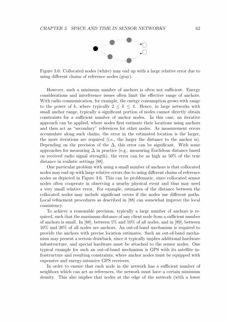
CHAPTER 3. SPACE AND TIME IN SENSOR NETWORKS 62
Figure 3.6: Collocated nodes (white) may end up with a large relative error due tousing different chains of reference nodes (gray).
However, such a minimum number of anchors is often not sufficient. Energyconsiderations and interference issues often limit the effective range of anchors.With radio communication, for example, the energy consumption grows with rangeto the power of k, where typically 2 ≤ k ≤ 4. Hence, in large networks withsmall anchor range, typically a significant portion of nodes cannot directly obtainconstraints for a sufficient number of anchor nodes. In this case, an iterativeapproach can be applied, where nodes first estimate their locations using anchorsand then act as “secondary” references for other nodes. As measurement errorsaccumulate along such chains, the error in the estimated location is the larger,the more iterations are required (i.e., the larger the distance to the anchor is).Depending on the precision of the ∆, this error can be significant. With someapproaches for measuring ∆ in practice (e.g., measuring Euclidean distance basedon received radio signal strength), the error can be as high as 50% of the truedistance in realistic settings [88].
One particular problem with using a small number of anchors is that collocatednodes may end up with large relative errors due to using different chains of referencenodes as depicted in Figure 3.6. This can be problematic, since collocated sensornodes often cooperate in observing a nearby physical event and thus may needa very small relative error. For example, estimates of the distance between thecollocated nodes may include significant errors if the nodes use different paths.Local refinement procedures as described in [88] can somewhat improve the localconsistency.
To achieve a reasonable precision, typically a large number of anchors is re-quired, such that the maximum distance of any client node from a sufficient numberof anchors is small. In [88], between 5% and 10% of all nodes, and in [89], between10% and 20% of all nodes are anchors. An out-of-band mechanism is required toprovide the anchors with precise location estimates. Such an out-of-band mecha-nism may present a serious drawback, since it typically implies additional hardwareinfrastructure, and special hardware must be attached to the sensor nodes. Onetypical example for such an out-of-band mechanism is GPS with its satellite in-frastructure and resulting constraints, where anchor nodes must be equipped withexpensive and energy-intensive GPS receivers.
In order to ensure that each node in the network has a sufficient number ofneighbors which can act as references, the network must have a certain minimumdensity. This also implies that nodes at the edge of the network (with a lower

CHAPTER 3. SPACE AND TIME IN SENSOR NETWORKS 63
(a) (b)
d dd d
1 2 1 2
ee
1 2
2
1 2
2
Figure 3.7: Localization error depends on the constellation of reference nodes.
number of neighbors) typically experience a reduced precision. Network densityis particularly important if the collected constraints are loose, since then manyconstraints are needed to achieve precise location estimates. In [88], for example,each node must have an average of 7 to 12 neighbors on average in order to achievea reasonable precision.
The arrangement of the anchors is also of importance for the achieved precisionof localization in spacetime. Obviously, anchors should be evenly distributed acrossthe sensor network in order to ensure that any node has a sufficient number of an-chors in its vicinity. However, also the relative arrangement of anchors with respectto each other has an influence on the localization accuracy. For example, collinearanchors (i.e., anchor nodes that fall on a line in 3D space) and also approximatelycollinear anchors result in significantly reduced precision for localization in space.This is illustrated for localization in 2D in Figure 3.7. In part (a), the error e2 indistance measurement results in a small error in the estimated location (dotted cir-cle) w.r.t. the actual location of the node (solid circle). In part (b), where anchornodes are almost collinear (i.e., fall on a point in 2D), the same error e2 results ina much larger error in the estimated location.
3.4.2 Energy and Other Resources
As noted in Section 3.2.5, it is quite common that applications do only require avery limited scope and lifetime of localization, where actual scope and lifetime re-quirements depend on the occurrence of events in the physical environment. Hence,a significant amount of resources and energy could be saved if localization is onlyperformed where and when needed and with the required precision.
However, distributed algorithms for localization in spacetime are often not wellsuited for on-demand localization. This is due to two main reasons. Firstly, lo-calization of a single node typically requires the cooperation of many other nodesto act as references for obtaining constraints. For on-demand localization, (re-cursively) providing a sufficient number of reference nodes on-demand would beneeded. However, managing this process is a complex task. For example, as notedin the previous section, the number and relative arrangement of the anchors must beconsidered by such mechanisms, as this is crucial for the achieved precision. More-

CHAPTER 3. SPACE AND TIME IN SENSOR NETWORKS 64
over, such selective localization may induce significant management overheads.Secondly, many algorithms require a significant amount of convergence time for
achieving the requested precision. For example, [60] reports a convergence timeof 10 minutes in a network of only few tens of nodes. Hence, if a node requestslocalization, a significant amount of time will elapse before a location estimate withsufficient precision can be provided.
3.4.3 Network Dynamics
In Section 2.6.2 we discussed various effects of network dynamics found in sensornetworks. These effects may have a significant impact on the performance andapplicability of localization algorithms.
An important implicit assumption of many localization algorithms is that beforethe location of a node can be estimated, the node must obtain constraints involvinga sufficient number of reference nodes. These references in turn must also be ableto obtain constraints from a sufficient number of other reference nodes, and soon. Overall, in order to locate a node, there must be “constraint paths” from aclient node to a sufficient number of anchors. This typically means that a sufficientportion of the network must be connected before localization can be performed.
However, a number of application projects (e.g., [48]) explore settings, wheresensor nodes are mobile and network connectivity is sporadic. In such settings,there may not be a network connection between nodes that require localizationin spacetime with respect to a common coordinate system. Algorithms with theabove implicit connectivity assumption cannot be used for such applications. Wewill address this problem in Chapter 4.
As noted in the previous section, many algorithms take a significant amount ofconvergence time before delivering the requested precision. It is typically assumedthat the network remains stable during the execution of the algorithm. However,node mobility and other effects of network dynamics may invalidate this assump-tion. This may lead to significantly increased convergence times (see, e.g., [98]),or may also prevent the algorithm from converging at all. In the latter case, theeffective precision may reduce significantly.
Some algorithms construct an explicit overlay topology as noted in Section3.3.4. Network dynamics may break these topologies or make them inefficient.Maintaining these topologies under a high degree of network dynamics may becomean unacceptable resource overhead.
3.4.4 Configuration
Localization algorithms may require a number of configuration parameters whosevalues differ from node to node. In order to allow unattended operation, configu-ration must be performed with little or no support from human operators.
Typical examples for configuration parameters are the set of reference nodes touse, network link calibration parameters (e.g., minimum delay of a wireless link),

CHAPTER 3. SPACE AND TIME IN SENSOR NETWORKS 65
and sensor calibration parameters (e.g., for distance measurements). While someof these parameters can be automatically configured and adapted, this is not soeasy for other parameters. For example, calibration may be a particularly trickyissue in sensor networks, because typical low-cost sensors used on sensor nodes arevery sensitive to environmental parameters such as temperature and humidity. Ifthese sensors are exposed to a harsh and dynamic physical environment, the out-put of the sensors includes significant errors. In [108], for example, the authorsobserved an average error of approx. 75% for distance measurements with uncali-brated sensors based on time of flight of an ultrasound signal. Additionally, sensororientation, wear, and dirt lead to systematic but dynamically changing errors.Hence, calibration parameters often cannot be statically configured, but must bedynamically updated to reflect the changing setup.
3.5 Summary
This chapter discussed issues related to time and space in wireless sensor networks.We presented a common framework that supports a unified view on space andtime. In particular, we presented applications of space and time and classifiedthese into three broader categories: applications related to interfacing a sensornetwork to an external observer, applications related to interfacing a sensor net-work to the observed real-world, and applications related to coordination amongsensor nodes. We also discussed various requirements and general approaches thatapply both to time synchronization and localization: internal vs. external localiza-tion/synchronization, local vs. global scales, the use of point estimates vs. boundsto represent points in time/space, the need for synchronized points vs. distances,scope and lifetime of synchronization/localization, precision, and other QoS re-quirements. Then we considered distributed algorithms for synchronization andlocalization and pointed out five common structural elements of many algorithms:bootstrapping, obtaining constraints, combining constraints, selecting constraints,and maintaining localization/synchronization over time. We then showed thatthese algorithms are affected by a number of limitations and trade-offs in fourbroader categories: with respect to anchor infrastructures, energy and resourceconsumption, network dynamics, and with respect to configuration.

Chapter 4
Time Synchronization
The significance of physical time for sensor networks has been reflected by thedevelopment of a number of time synchronization algorithms in the recent past.However, most of these approaches have been designed for “traditional” sensornetworks, covering only a small region of the design space discussed in Section 2.2.We will identify an important region in the design space that is not sufficientlysupported by existing approaches. In order to fill this gap, we present and evaluatean algorithm called “Time-Stamp Synchronization”.
We begin our discussion in Section 4.1 by studying fundamental system modelsand by presenting concrete algorithmic techniques for synchronization. The discus-sion will be structured according to the common framework we developed in theprevious chapter. Referring to these techniques, we present existing algorithms fortime synchronization in Section 4.2. Our algorithm will be motivated and presentedin Sections 4.3 and 4.4.
4.1 Background
This section reviews models and concepts for time synchronization. The discussionis structured according to Section 3.3.
4.1.1 Clock and Communication Models
In the following two subsections we discuss models of communication and of hard-ware clocks. Communication is fundamental for measuring temporal relationshipsamong nodes. Hardware clocks are an important tool for maintaining synchroniza-tion over time.
Clock Models
Most computer systems in use today are based on clocked circuits and hence con-tain so-called digital clocks. Such hardware clocks are a valuable tool for time
66

CHAPTER 4. TIME SYNCHRONIZATION 67
synchronization, since they can be used to maintain synchronization over time asdiscussed in Section 3.3.5.
A typical hardware clock consists of a quartz-stabilized oscillator and a counterthat is incremented by one every oscillation period (e.g., upon detection of a fallingor rising edge). If the periodic time T of the oscillator is known, the counter h canbe used to obtain approximate measurements of real-time intervals in multiples ofT .
More formally, the clock counter displays value h(t) at real time t and is in-cremented by one at a frequency of f . The rate of the counter is defined asf(t) = dh(t)/dt. An ideal digital clock would have a rate of 1 at all times. How-ever, the periodic time of the oscillator and hence the clock rate depend on variousparameters such as age of the quartz, supply voltage, environmental temperatureand humidity. This so-called clock drift is formally defined as the deviation of therate from 1 or
ρ(t) = f(1)− 1 (4.1)
Since sensor nodes are typically operated under a well-defined ranges of the aboveparameters, it is reasonable to assume a maximum possible drift ρmax, such that
|ρ(t)| ≤ ρmax (4.2)
for all t. Typical values for ρmax are 1ppm to 100ppm, where 1ppm = 10−6.Some researchers make additional assumptions about the clock rate such as
bounded drift variation or constant clock rate. The latter may not be a reasonablemodel for sensor networks that are exposed to significant changes of environmentalparameters.
Communication Models
Obtaining temporal constraints (cf. Section 3.3.2) is typically implemented bycommunication among sensor nodes. There are three major characteristics of com-munication that affect time synchronization.
Firstly, a communication network has the multicast/broadcast capability if asingle message can be received by multiple/all nodes within the communicationrange of the sender. Since commonly used sensor nodes use radio communica-tion, message broadcasts are typically supported. Broadcasts can, for example,be exploited to synchronize an arbitrary number of nodes with a fixed number ofmessages.
Secondly, a communication link is said to be symmetrical if it can be used inboth directions. A link is asymmetrical if it can be used in one direction only. Forexample, some algorithms rely on the ability to measure round-trip-delays, whichrequires symmetrical links (cf. Section 2.6.2).
Thirdly, the latency or delay characteristics of a communication link are ofutmost importance for time synchronization. Known constant delays can be easilycompensated by including a respective constant offsets in time synchronization

CHAPTER 4. TIME SYNCHRONIZATION 68
algorithms. However, the latency of a communication link typically varies overtime (cf. Section 2.6.2). These variable delays can be attributed to four majorsources:
• Send time, lasting from when the application issues a “send” command to theoperating system, until when a raw network message has been constructedthat could be delivered to the communication medium. Variable delays resultfrom operating system context switches, network protocol processing, andfrom hardware interrupts.
• Medium access time. The communication medium is typically shared bymany network nodes, such that immediate access may not be possible, causingadditional variable delays. For example, random backoff mechanisms areoften used to resolve collisions. Since the channel bandwidth is rather low forsensor networks (few tens of kilobit per second), this delay component mayvary between zero and few tens of milliseconds.
• Propagation time. The time it takes for the radio signal to travel from thesender to the receiver depends on the distance between the nodes. These de-lays are often negligible for radio communication due to the high propagationspeed and since the communication range is often rather small (few tens ofmeters). Typical values are between zero and few tens of nanoseconds.
• Receive time, lasting from the arrival of the signal at the antenna of the re-ceiver, until when the application is notified about the arrival of the message.There is often a variable delay in the order of the duration of one bit untilthe radio hardware triggers a receive interrupt to the processor. As for thesend time, additional variable delays are caused by context switches, networkprotocol processing, and interrupts.
There are two important approaches to eliminate or to limit the impact of thesevariable delays. The first approach is to implement time synchronization in theMAC layer, thus eliminating send and medium access time, as well as most of thereceive time. Another approach is to synchronize a set of nodes by sending a singlebroadcast message to them, such that all nodes experience identical send time andmedium access time.
4.1.2 Obtaining Constraints
As discussed in Section 3.3.2, a client node that is to be synchronized has to obtaintemporal constraints on its local time with respect to a time scale defined by areference node. Such a constraint typically involves the state S of the referencenode and a temporal relationship ∆ between the client node and the reference node.For time synchronization, S typically consists of the local time hr of the referencenode, and ∆ is a delay for sending a message from the reference node to the clientnode or vice versa. The client node can also refer to its current local time hc that

CHAPTER 4. TIME SYNCHRONIZATION 69
R C
t 1
t 2
R C
t 1
t 2
t 3
t 2t 1
(a) (b) (c)
R C
B
Figure 4.1: Obtaining temporal constraints. (a) Unidirectional, (b) round-trip, and(c) reference broadcast.
is defined by its (unsynchronized) hardware clock. The goal is to derive constraintson the synchronized time h′
c of the client node.Figure 4.1 illustrates three basic approaches for obtaining such constraints. In
(a), the reference node R sends a single message to the client node C at real timet1, which is received by the client node at t2. Note that nodes do not have access toreal time t, only hr(t1) and hc(t2) (i.e., the values of the local clock counters at therespective real-time instants) is known to them. If the message delay d = t2 − t1were known, a valid constraint would be h′
c(t2) = hr(t1) + d. Here, hr(t1) wouldrepresent the state information S of the reference node, and d would representthe temporal relationship ∆. However, d is unknown to both reference and clientnodes. If upper and lower bounds dmin < d < dmax are known, the following wouldbe possible constraints:
h′c(t2) > hr(t1) (4.3)
h′c(t2) > hr(t1) + dmin (4.4)
h′c(t2) < hr(t1) + dmax (4.5)
h′c(t2) = hr(t1) (4.6)
h′c(t2) = hr(t1) + dmin (4.7)
h′c(t2) = hr(t1) + dmax (4.8)
h′c(t2) = hr(t1) + (dmin + dmax)/2 (4.9)
Note that constraints 4.3-4.5 are correct bounds, while constraints 4.6-4.9 are onlyapproximations. Perhaps the most commonly used constraint is 4.6, because itdoes not require knowledge of bounds and is a good approximation if MAC layertechniques are used to eliminate send, medium access, and receive times. Note thatthis technique can be used to synchronize an arbitrary number of clients with onebroadcast message.

CHAPTER 4. TIME SYNCHRONIZATION 70
In Figure 4.1 (b), the client node first sends a request message to the reference,which is immediately answered with a reply (an additional delay between receiptof the request and sending of the reply can be easily measured and compensated).Here, some notable constraints are:
h′c(t3) > hr(t2) (4.10)
h′c(t3) > hr(t2) + dmin (4.11)
h′c(t3) < hr(t2) + (hc(t3)− hc(t1)) (4.12)
h′c(t3) = hr(t2) + (hc(t3)− hc(t1))/2 (4.13)
Note that constraints 4.10 and 4.12 give upper and lower bounds on h′c(t3) without
knowledge of dmin and dmax. Constraint 4.13 is a good approximation if bothmessages have about the same delay (i.e., t2− t1 ≈ t3− t2). Note that the numberof required messages grows linearly with the number of clients.
In Figure 4.1 (c), an additional beacon node B sends a broadcast to both thereference and the client node. A commonly used constraint with this approach is
h′c(t2) = hr(t1) (4.14)
This is a good approximation, since both nodes will receive the message almost con-currently as explained in Section 4.1.1. Note that exact bounds cannot be derivedunless bounds on the message delay are known a priori. A single broadcast messagecan be used to synchronize an arbitrary number of clients, but additional messageexchanges are required to transmit hr(r1) from the reference to the client(s).
4.1.3 Combining Constraints
Although a single constraint may be sufficient to derive synchronized time h′c at
the client node, multiple constraints can significantly improve the achieved pre-cision. Let us first consider the case where multiple constraints are available onh′
c(t0) for some real-time instant t0. This might for example be achieved by con-currently requesting synchronization with multiple reference nodes. As discussedin the previous section, these constraints are either bounds or approximations.
If bounds are used, each pair of lower and upper bound can be consideredas an interval. The intervals are open at one end if only lower or upper boundsare available. The combined interval is then computed as the intersection of allavailable intervals. If some or all intervals are closed, then this intersection may beempty. Hence, outlier rejection is often performed to eliminate intervals that wouldlead to an empty intersection. In general, different subsets of intervals result in anon-empty intersection. Various criteria can be applied to select such a subset, forexample, minimizing the number of rejected intervals, or minimizing the length ofthe intersection interval.
If approximations are used, the average of all constraints can serve as the com-bined constraint. Outlier rejection can also be performed in order to reject false

CHAPTER 4. TIME SYNCHRONIZATION 71
h (t)c
h’ (t)c
h (t)c
h’ (t)c
(a) (b)
Figure 4.2: Prediction of synchronized time using a hardware clock. (a) Pointestimates, (b) bounds.
constraints. One criterion for this would be to remove all constraints that deviatefrom the average by more than a certain threshold.
Sometimes it is possible to derive a confidence value for each constraint.The higher the confidence value, the better the constraint. With the round-trip technique in Figure 4.1 (c), for example, the inverse of the round-trip time1/(hc(t3) − hc(t1)) could be used as a confidence for the approximation h′
c(t3) =hr(t2) + (hc(t3)− hc(t1))/2. If such confidence values are available, a weighted av-erage can be computed. The confidence values can also be used to control outlierrejection.
4.1.4 Maintaining Synchronization
In the previous section we described how constraints on h′c(tx) can be obtained for a
real-time instant tx. These constraints directly result in a estimate for the synchro-nized time of the client node at real time tx. In order to obtain such an estimatefor another instant ty, the procedure of obtaining and combining constraints canbe repeated as discussed in Section 3.3.5. However, there are two problems withthis approach. Firstly, as discussed in Section 3.3.5, such an approach may exhibitsignificant overheads in terms of communication and computation. Secondly, theapplication may request synchronized time at tx, but due to processing delays theconstraints refer to tx + ε. In Figure 4.1 (a), for example, after the client applica-tion requests synchronized time at t0, the client node must wait until it receives asynchronization message from the reference node in order to obtain constraints onh′
c(t2), where t2 > t0.In order to approach these problems, the client node may use its local hardware
clock to predict h′c(ty), where no measured constraints are available for real time
ty. For this, a mapping from hc(t) to h′c(t) must be derived, given a set of measured
constraints on h′c(txi
) for different real-time instants txias illustrated in Figure 4.2.
In (a), each circle indicates a data point (hc(txi), h′
c(txi)) where a point estimate for
h′c(txi
) is known. In (b), lower (5) and upper bounds (4) for h′c(txi
) are known.

CHAPTER 4. TIME SYNCHRONIZATION 72
PhaseDetector
VariableFrequencyOscillator
Filter
h (t)c
ch’’ (t)h’ (t )
ixc
Figure 4.3: Using a phase-locked loop to establish a mapping between hardwareclock and synchronized time.
Various methods can be applied to derive the desired mapping of hc(t) to h′c(t),
given the above sets of constraints. A commonly used approach is to assume alinear relationship
h′c(t) = αhc(t) + β (4.15)
Note that α can be interpreted as the relative drift or rate difference betweensynchronized time and the hardware clock, and β indicates the offset betweensynchronized time and the hardware clock. Once α and β are known, the linearfunction 4.15 can be used to derive the current (predicted) synchronized time usingthe current hardware clock reading.
Line fitting techniques such as linear regression can be used to obtain estimatesfor α and β as illustrated by the line in Figure 4.2 (a). If bounds are used, asteepest and a flattest line can be fitted as illustrated by the dashed in lines in(b). The resulting values for α and β for the two lines can then be used as lowerand upper bounds for rate and offset differences between synchronized time andthe hardware clock. Alternatively, the line defined by the average of the α and βvalues of the two lines can be used. Yet another approach is the use of convex hulls,where two lines are fitted such that they cut off minimal half planes that containall upper and all lower bounds, respectively. This is illustrated by the solid linesin Figure 4.2 (b). Note that the latter technique can also be applied if only loweror upper bounds are available.
An important question with the above techniques is how many data points (i.e.,constraints) should be included in the line fitting procedure. With small numbers,few outliers can have a significant impact on the fitting result. This can be dilutedby including a larger number of data points, which, however, results in increasedmemory footprint.
In practice, the relationship between synchronized time and hardware clock isoften not linear. By repeating the line fitting procedure frequently, a piecewiselinear approximation of that nonlinear relationship can be achieved. This approx-imation is the better, the fewer data points are included in each fitting procedure.Often it is mandatory to ensure that this piecewise approximation is continuous,which may require the introduction of additional constraints on the fitted lines.
A different approach to derive a mapping of hc(t) to h′c(t) is the use of phase-
locked loops (PLL). As depicted in Figure 4.3, a PLL consists of at least three

CHAPTER 4. TIME SYNCHRONIZATION 73
(a) (b) (c) (d)
Figure 4.4: Commonly used overlay topologies. (a) Stars, (b) tree, (c) hierarchy,and (d) clusters.
components. A variable frequency oscillator (VFO) is a component that producesan estimation h′′
c (t) for synchronized time h′c(t). The frequency dh′′
c (t)/dt can becontrolled by an input signal of the VFO. The generation of the output signal isusually based on the hardware clock signal hc(t), which therefore represents thesecond input to the VFO. The phase detector (PD) estimates the phase offset ofits two input signals and generates an output signal that is proportional to theobserved phase difference. The first input of the PD is the sequence of estimatesh′
c(txi), the second input is the output h′′
c (t) of the VFO. The output of the PD isfed to a filter that integrates the observed phase differences over time and producesan output signal to control the frequency of the VFO. Overall, a PLL can beconsidered as a feedback loop that adjusts the frequency and phase of the VFOto the discrete input signal h′
c(txi). Hence, the output h′′
c (t) of the VFO is anapproximation of synchronized time h′
c(t).In contrast to the line fitting approach, a PLL requires only minimal state
information and does not assume a linear relationship. However, due to the delayintroduced by the filter, it may take minutes before the VFO output converges toa stable frequency.
Note that both of the above approaches are a combination of prediction anddead reckoning (cf. Section 3.3.5). The hardware clock can be considered a “timesensor” that is calibrated using the observed past behavior of synchronized time.
4.1.5 Selecting Constraints
As discussed in Section 3.3.4, there are two basic approaches to control the selectionof reference nodes by a client node: structured and unstructured approaches. Withstructured approaches, an overlay topology is constructed and maintained, whichcan be interpreted as a subgraph of the network. A client node then only consid-ers neighbors in this overlay topology as potential references. With unstructuredapproaches, a client node may consider any of its neighbors as references.
As depicted in Figure 4.4, commonly used overlay topologies are stars, trees,hierarchies, and clusters. With stars, a number of anchor nodes (black) are dis-tributed across the network, such that each client node (white) has one or moreanchors in its one-hop neighborhood. The anchors are synchronized with each

CHAPTER 4. TIME SYNCHRONIZATION 74
other by means of an out-of-band mechanism. With trees, a single anchor nodeforms the root of a spanning tree. The nodes in the tree synchronize top-down withtheir parents, such that each node has exactly one reference node. Hierarchies aredirected acyclic graphs with one or more anchors at the top. Nodes synchronizetop-down with their parents. With clustering, nodes are grouped into clusters, suchthat adjacent clusters share common gateway nodes (gray). The nodes in a clus-ter are synchronized in some way with each other. Gateway nodes independentlyparticipate in the synchronization process of each adjacent cluster, such that theycan translate between the time scales of the clusters they participate in.
4.2 Related Work
This section presents and discusses existing approaches for time synchronization.We first discuss related and influential approaches from other domains, pointing outtheir shortcomings in the context of sensor networks. Our main focus is, however,on algorithms which have been specifically developed for sensor networks. Theseare based on the models and concepts presented in the previous section.
4.2.1 Logical Time
Logical time [54, 64] provides mechanisms to time-stamp events (e.g., receipt orsending of a message). For example, C(e1) is the logical time stamp of event e1. Ifa second event e2 is causally dependent on e1 (i.e., e1 → e2), then C(e1) < C(e2)will hold with respect to some ordering relation “<” on time stamps. Two eventsare causally dependent if they happened in the same process or if there is a messagepath connecting e1 and e2.
In sensor networks, where sensor events are triggered by real-world phenomena,sensor events are only causally related if they have been generated by the samesensor node. Hence, temporal reasoning on events originating from different nodescannot be supported by logical time. Moreover, it is often necessary to measure theamount of real-time elapsed between two sensor events, which cannot be achievedwith logical time. Therefore, physical time must be used to relate events in thephysical world.
4.2.2 Offline Time Synchronization
Time synchronization algorithms typically perform synchronization during the ex-ecution of a distributed application. Offline time synchronization performs syn-chronization only after a distributed application has finished execution. For this,each node logs events (e.g., message sent, message received) during the executionof the application. Each logged event is tagged with the time of occurrence usingthe unsynchronized hardware clock of the node. This results in an event log foreach node. These logs are than provided as input to an offline time synchroniza-

CHAPTER 4. TIME SYNCHRONIZATION 75
tion algorithm. For each pair of nodes, the algorithm then computes a coordinatetransformation between the local timescales of the nodes.
Such event logs are collected over extended periods of time (e.g., hours). Exist-ing algorithms [5, 31] typically assume that the rate difference between the hard-ware clocks and the message delays are constant during the logging period.
In the context of sensor networks, offline approaches are of limited applicability,since synchronized time is often required during the execution of an application.Secondly, both message delays and clock rates may be subject to significant varia-tion in sensor networks (cf. Section 4.1.1).
4.2.3 Network Time Protocol (NTP)
NTP [68] has been designed for large-scale networks with a rather static topology(such as the Internet). Nodes are externally synchronized to a global referencetime that is injected into the network at many places via a set of master nodes,so-called “stratum 1” servers. These master nodes are synchronized out of band,for example via GPS. Nodes participating in NTP form a hierarchy: leaf nodes arecalled clients, inner nodes are called stratum L servers, where L is the level of thenode in the hierarchy. The parents of each node must be specified in configurationfiles at each node. A node in the hierarchy uses round-trip measurements to obtainbounds on synchronized time with respect to its parents. Outliers are removed fromthe resulting set of intervals. From the intersection of the remaining intervals, apoint estimate of synchronized time is computed and used as input for a PLL thateventually outputs synchronized time.
While NTP has been successfully applied in the Internet, it fails to meet manyof the technical challenges discussed in Section 2.6. Many of these limitations areclosely related to the issues discussed in Section 3.4.
Resource and energy constraints. Resource constraints may preclude the useof GPS or other technologies for out-of-band synchronization of NTP master nodes.NTP is also not optimized for energy efficiency, simply because this is not an issuein traditional distributed systems. Energy overhead in NTP results from severalsources. Firstly, the service provided by NTP typically cannot be dynamicallyadapted to the varying needs of an application. Hence, with NTP all nodes wouldbe continuously synchronized with maximum precision, even though only subsetsof nodes might occasionally need synchronized time with less-than-maximum pre-cision.
Secondly, NTP uses the processor and the network in ways that would lead tosignificant overhead in energy expenditure in sensor networks. For example, NTPmaintains a synchronized system clock by regularly adding small increments to thesystem-clock counter. This behavior precludes the processor from being switchedto a power-saving idle mode. In addition, NTP servers must be prepared to receivesynchronization requests at any point in time. However, constantly listening is anenergy-wise costly operation in sensor networks; many sensor-network protocols

CHAPTER 4. TIME SYNCHRONIZATION 76
therefore switch off the radio whenever possible.
Network dynamics. The operation of NTP is largely independent of the un-derlying physical network topology. In the NTP overlay hierarchy, a master and aclient can be separated by many hops in the physical network, even though theyare neighbors in the overlay hierarchy. As discussed in Section 2.6.2, multi-hoppaths may be very unstable and unpredictable in a sensor network. NTP, however,depends on the ability to accurately estimate the delay characteristics of multi-hopnetwork links.
NTP implicitly assumes that network nodes that shall be synchronized area priori connected by the network. However, this assumption may not hold indynamic sensor networks with mobile nodes as discussed in Section 2.6.2.
Infrastructure. In order to improve the precision and availability of synchro-nization in large networks, reference time is injected at many points into the net-work. Hence, any node in the network is likely to find a source of reference timein a distance of only a few hops. However, such an approach requires an externalinfrastructure of reference-time sources which have to be synchronized with someout-of-band mechanism. Where this is not feasible, NTP would have to operatewith a single master node, which uses its local time as the reference time. Inlarge sensor networks, the average path length from a node to this single masteris long, leading to reduced precision. If collocated nodes end up using differentsynchronization paths, they will be poorly synchronized (cf. Section 3.4.1).
Configuration. NTP requires the specification of one or more potential synchro-nization masters for each node. This is an appropriate solution for networks witha rather static topology, where configurations remain valid for extended periodsof time. In sensor networks, however, network dynamics necessitate a frequentadaptation of configuration parameters.
4.2.4 Time Synchronization for Sensor Networks
In this section we review time synchronization approaches that have been specif-ically devised for sensor networks. Note that most of these algorithms have beenproposed after our work presented in Section 4.4.
Reference-Broadcast Synchronization (RBS)
RBS [33] denotes some nodes as beacons which frequently broadcast messagesto a set of client nodes that should be synchronized as illustrated in Figure 4.1(c) on page 69. Clients that receive such a broadcast exchange their respectivereception times to obtain mutual constraints. Each client collects multiple suchconstraints and uses linear regression to compute relative time offsets and ratedifferences to the other client nodes. The offset and rate difference between a pair of

CHAPTER 4. TIME SYNCHRONIZATION 77
client nodes defines a coordinate transformation between the local time scales (i.e.,coordinate systems) of these nodes. To extend this scheme to multi-hop networks,the network is clustered such that a single beacon can synchronize all nodes inits cluster. Gateway nodes that participate in two or more clusters independentlytake part in the reference-broadcast procedure of all adjacent clusters. By knowingoffsets and rate differences to nodes in all clusters, gateway nodes can computecoordinate transformations between all adjacent clusters. Time synchronizationacross multiple hops is then provided by transforming clock readings between thelocal time scales (i.e., coordinate systems) of the nodes.
In experiments it has been shown that adjacent Berkeley Motes can be synchro-nized with an average error of 11 µs by using 30 broadcasts. Over multiple hops,the average error grows with O(
√n), where n is the number of hops.
Tiny-Sync and Mini-Sync (TS/MS)
Tiny-Sync and Mini-Sync [95] are methods for pairwise synchronization of sensornodes. Both Tiny-Sync and Mini-Sync use multiple round-trip measurements anda line-fitting technique to obtain the offset and rate difference of the two nodes.For this, a constant clock rate is assumed. To obtain data points for line fitting,multiple round-trip measurements are performed as depicted in Figure 4.1 (b) onpage 69. Each round-trip measurement is used to obtain lower and upper bounds onh′
c(t). Then, the line-fitting technique depicted in Figure 4.2 (b) on page 71 is usedto calculate two lines with minimum and maximum slope. Slope and axis interceptof these two lines then give bounds for the relative offset and rate difference of thetwo nodes. The line with average slope and intercept of the two lines is then usedas the offset and rate difference between the two nodes.
Note that each of the two lines is unambiguously defined by two (a priori un-known) data points. The same results would be obtained if the remaining datapoints were eliminated. Since the computational and memory overhead dependson the number of data points, it is a good idea to remove as many data points aspossible before the line fitting. Tiny-Sync and Mini-Sync only differ in this elimi-nation step. Essentially, Tiny-Sync uses a heuristic to keep only two data points foreach of the two lines. However, the selected points may not be the optimal ones.Mini-Sync uses a more complex approach to eliminate exactly those points thatdo not change the solution. Hence, Tiny-Sync achieves a slightly suboptimal so-lution with minimal overhead, Mini-Sync gives an optimal solution with increasedoverhead.
Measurements on a 802.11b network with 5000 data points resulted in an offsetof 945 µs (3230 µs) and a rate difference of 0.27 ppm (1.1 ppm) for adjacent nodes(nodes five hops away).
Lightweight Time Synchronization (LTS)
LTS [101] is a synchronization technique that provides a specified precision withlittle overhead, rather than striving for maximum precision.

CHAPTER 4. TIME SYNCHRONIZATION 78
Two algorithms are proposed: one that operates on demand for nodes that ac-tually need synchronization, and one that proactively synchronizes all nodes. Bothalgorithms assume the existence of one or more master nodes that are synchronizedout-of-band to a reference time. The proactive algorithm proceeds by constructingspanning trees with the masters at the root by flooding the network. In a sec-ond phase, nodes synchronize to their parents in the tree by means of round-tripsynchronization. The synchronization frequency is calculated from the requestedprecision, from the depth of the spanning tree, and from the drift bound ρmax.
The on-demand version also assumes the existence of one or more master nodes.When a node needs synchronization, it sends a request to one of the masters usingany routing algorithm (this is not further specified). Then, along the reverse pathof the request message, nodes synchronize using round-trip measurements. Thesynchronization frequency is calculated as in the proactive version described above.In order to reduce synchronization overhead, each node may ask its neighborsfor pending synchronization requests. If there are any such requests, the nodesynchronizes with the neighbor, rather than executing an independent multi-hopsynchronization with a reference node.
The overhead of the algorithms was examined in simulations with 500 nodesuniformly placed in a 120 m × 120 m area, a target precision of 0.5 s, and a durationof 10 hours. The centralized algorithm performed an average of 36 pairwise syn-chronizations per node. The distributed algorithm executed 4-5 synchronizationson average per node if 65% of all nodes request synchronization.
Timing-Sync Protocol for Sensor Networks (TPSN)
TPSN [38] provides synchronization for a whole network. First, a node is electedas a synchronization master (details for this are not specified), and a spanning treewith the master at the root is constructed by flooding the network. In a secondphase, nodes synchronize to their parents in the tree using round-trip measure-ments. Synchronization is performed in rounds and initiated by the root broad-casting a synchronization-request message to its children. Each child then performsa round-trip measurement to synchronize with the root. Nodes further down inthe tree overhear the messages of their parents and start synchronization whentheir parents have synchronized. To eliminate message-delay uncertainties, time-stamping for the round-trip measurements is done in the MAC layer. In case ofnode failures and topology changes, master election and tree construction must berepeated.
Measurements showed that two adjacent Berkeley Motes can be synchronizedwith an average error of 16.9 µs, which is a worse figure than the 11 µs given forRBS in [33]. However, the authors of [38] claim that a re-implementation of RBSon their hardware resulted in an average error of 29.1 µs between adjacent nodes,effectively claiming that TPSN is about twice as precise as RBS.

CHAPTER 4. TIME SYNCHRONIZATION 79
TSync
TSync [26] provides two protocols for external synchronization: the Hierarchy Ref-erencing Time Synchronization Protocol (HRTS) for proactive synchronization ofthe whole network, and the Individual-Based Time Request Protocol (ITR) for on-demand synchronization of individual nodes. Both protocols use an independentradio channel for synchronization messages in order to avoid inaccuracies due tovariable delays introduced by packet collisions. In addition, the existence of one ormore master nodes with access to a reference time is assumed.
With HRTS, a spanning tree with the master at the root is constructed. Then,the master uses the reference broadcasting technique illustrated in Figure 4.1 (c)on page 69 to synchronize its children. Each child node now repeats the procedurefor its subtree.
Measurements in a network of MANTIS sensor nodes showed a mean synchro-nization error of 21.2 µs (29.5 µs) for two adjacent nodes (nodes three hops away).For comparison, RBS was also implemented, giving an average error of 20.3 µs(28.9 µs).
Interval-Based Synchronization (IBS)
Interval-based synchronization was first proposed in [63], where a bounded-driftmodel is assumed. The network nodes perform external synchronization by main-taining a lower and upper bound on the current time. During communication be-tween two nodes, the bounds are exchanged and combined by choosing the largerlower and the smaller upper bound. This amounts to intersecting the time intervalsdefined by each pair of bounds. Between communications, each node advances itsbounds according to the elapsed real time and the known drift bounds. In [91], themodel was refined by including bounded drift variation and fault-tolerance.
In [15], the simple approach from [63] was shown to be worst-case-optimal,where the worst case is the one where all clocks run with maximal drift. A con-siderable improvement in the synchronization quality can be achieved by havingeach node store, maintain, communicate, and use the bounds from its last com-munications with other nodes. In [65], it was shown that optimal interval-basedsynchronization can only be achieved by having nodes store and communicate theirentire history. Obviously, this becomes prohibitive with growing network size andlifetime. In realistic settings, the value of a piece of history data decreases rapidlywith its age. Therefore, efficient average-case-optimal synchronization can be ob-tained by using only recent data.
Flooding Time-Synchronization Protocol (FTSP)
FTSP [60] can be used to synchronize a whole network. The node with the low-est node ID is elected as the anchor whose local time serves as a reference forsynchronization. If this node fails, then the node with the lowest ID in the re-maining network is elected as the new anchor. The anchor periodically broadcasts

CHAPTER 4. TIME SYNCHRONIZATION 80
a synchronization message that contains its current local time. Nodes which havenot received this message yet use the message contents to derive a constraint andbroadcast the message to its neighbors. Each node collects eight such constraintsand uses linear regression on these eight data points to estimate time offset and ratedifference to the anchor. The algorithm is repeatedly executed to maintain syn-chronization over time. Time-stamping is performed in the MAC layer to minimizedelay variability.
Measurements were performed in an eight-by-eight grid of Berkeley Motes,where each Mote has a direct radio link to its eight closest neighbors. With thissetup, the network synchronized in 10 minutes to an average (maximum) synchro-nization error of 11.7 µs (38 µs), giving an average error of 1.7 µs per hop.
Asynchronous Diffusion (AD)
AD [56] supports the internal synchronization of a whole network. The algorithmis very simple: each node periodically sends a broadcast message to its neighbors,which reply with a message containing their current time. The receiver averagesthe received time stamps and broadcasts the average to the neighbors, which adoptthis value as their new time. It is assumed that these operations are atomic, thatis, the averaging operations of the nodes must be properly sequenced.
Simulations with a random network of 200 static nodes showed that the syn-chronization error decreases exponentially with the number of rounds.
Time Diffusion Synchronization (TDP)
TDP [98] supports the synchronization of a whole network. Initially, a set of masternodes is elected. For external synchronization, these nodes must have access to aglobal time. This is not required for internal synchronization, where masters areinitially unsynchronized.
Master nodes then broadcast a request message containing their current time,and all receivers send back a reply message. Using these round-trip measurements,a master node calculates and broadcasts the average message delay and standarddeviation. Receiving nodes record these data for all leaders. Then, the receiversturn themselves into so-called “diffused leaders” and repeat the procedure. Theaverage delays and standard deviations are summed up along the path from themasters. The diffusion procedure stops at a given number of hops from the masters.
All nodes have now received from one or more masters m the time hm(t0) at theinitial leader, the accumulated message delay ∆m, and the accumulated standarddeviation βm. A clock estimate is computed as
∑m ωm(hm(t0) + ∆m), where the
weights ωm are inversely proportional to the standard deviation βm. After all nodeshave updated their clocks, new masters are elected and the procedure is repeateduntil all node clocks have converged to a common time.
In a simulation with 200 static nodes with 802.11 radios and a delay of 5 sec-onds between consecutive synchronization rounds, the deviation of time across thenetwork dropped to 0.6 seconds after about 200 seconds.

CHAPTER 4. TIME SYNCHRONIZATION 81
1
2
E 1
3
1
2
E 2
3
1
2
3
E 2
1
2
3
E1
(a) (b) (c) (d)
Figure 4.5: Message transport across partition boundaries. (a-b) Sensor nodes 1and 2 collect sensor readings while disconnected from the network. (c-d) Later,sensor nodes 1 and 2 report their findings to node 3 for data fusion. At no pointin time there is a network connection between node 1 and 2.
4.3 Problem Statement
One of the main uses of synchronized time in wireless sensor networks is time-stamping of events to support data evaluation, aggregation, and fusion as men-tioned in 3.1. For this, a sensor node i generates a time stamp Si(tE) that rep-resents the real-time instant tE when event E occurred. This time stamp maybe included in network messages along with other parameters that describe theobserved event. When a sensor node receives many such time stamps from one ormore sensor nodes (including itself), these time stamps should refer to a commontime scale, such that time stamps can be compared, ordered, etc.
One possible approach to the above problem is the use of time synchronizationamong all nodes of the network. Then, time-stamping can be implemented bysetting S(tE) := h′(tE). One of the time synchronization algorithms for sensornetworks discussed in Section 4.2 could then be used to provide synchronized time.However, we will show below that this approach cannot support a relevant classof applications. Our goal is the development of a time-stamping approach for theregion in the design space we will characterize below.
4.3.1 Intermittent Connectivity
None of the algorithms discussed in Section 4.2 can support networks with intermit-tent or sparse connectivity, where messages are relayed across temporary partitionsby mobile nodes as discussed in Section 2.6.2.
Consider for example the ZebraNet application discussed in Section 2.4.1, wherenodes are attached to wild animals, forming a network with sporadic connectivity.Figure 4.5 depicts, from left to right, four snapshots of such a network. At real-time t1 node 1 detects some event. At t2 node 2 detects another event. At t3 node2 passes by the mobile base station (node 3), a communication link is establishedand E2 is sent to the base station. At t4 node 1 passes by the base station, a linkis established and E1 is sent to the base station.

CHAPTER 4. TIME SYNCHRONIZATION 82
Now the base station wants to determine a temporal relationship among E1 andE2, for example, it might be necessary to determine whether E1 happened afterE2, or the time between the occurrence E1 and E2 might be of interest.
Note that there has not been a network connection between nodes 1 and 2before the occurrence of the events E1 and E2, so the clocks of the two nodescannot be synchronized with each other in advance to provide synchronized timefor time stamping.
4.3.2 Resource Efficiency
In many applications, relevant events occur rarely. In the bird monitoring applica-tion described in Section 2.4.1, a relevant event could be a bird leaving or enteringits burrow. Hence, synchronized time is only needed at rare occasions, namelywhere and when a relevant event occurs. A cross-layer approach (cf. Section 2.7.6)to time synchronization that provides synchronized time on demand only where andwhen needed can be expected to perform significantly better than using a general-purpose synchronization algorithm that runs independently of the time-stampingin the application layer.
4.3.3 Precision for Collocated Nodes
Many physical phenomena have a rather local geographical scope. Typically, onlygeographically collocated nodes have to cooperate in order to monitor such a phe-nomenon. These collocated nodes may require very precisely synchronized time inorder to aggregate or fuse sensory data. As discussed in Section 3.4.1, the precisionof anchor-based algorithms is determined by the placement of the anchors, suchthat collocated nodes may end up with an imprecise mutual synchronization. Alocalized, anchor-free algorithm (cf. Section 2.7.3) can be expected to give betterprecision for collocated nodes.
4.3.4 Correctness
Data fusion is often very sensitive to even small synchronization errors. Correctordering of events, for example, may be wrong if the synchronization error is largerthan the time between the occurrence of two events. A time synchronization al-gorithm that can provide guaranteed bounds on time stamps would be helpful forsuch applications.
4.4 Time-Stamp Synchronization
In this section we present an algorithm called “Time-Stamp Synchronization”(TSS), which is suitable for the time-stamping problem stated in the previoussection. This algorithm enables participating nodes to reason about sets of time
CHAPTER 4. TIME SYNCHRONIZATION 83
stamps (e.g., determine temporal ordering and time spans) received from arbitrarynodes even in the presence of intermittent network connectivity.
We will consider message flows in ad hoc sensor networks, which can be de-picted by (time-independent) message flow graphs, where the nodes of the graphcorrespond to network nodes, each equipped with its own clock. Paths in the graphcorrespond to possibly delayed message flows between the nodes (i.e., connectivitybetween the nodes may be intermittent). Without loss of generality, we will onlyconsider linear graphs as depicted in Figure 4.7. In case a message is broadcastto many nodes, the resulting graph can be considered as the union of many suchlinear graphs.
4.4.1 Algorithm Overview
The basic idea of the algorithm is not to synchronize the local clocks of the nodes,but instead generate time stamps using unsynchronized local clocks. When such“local” time stamps are passed between nodes as part of network messages, theyare transformed to the local time scale of the receiving node.
Time stamps are represented as intervals. With each transformation step, theuncertainty (i.e., length) of these intervals increases due to clock drift and delayuncertainties (cf. Section 4.1.1). In particular, each transformation between thetime scales of sender and receiver will consist of two steps: a transformation fromsender time scale to real time, and a transformation from real time to the receivertime scale.
Time-stamp transformation is achieved by determining the age of each timestamp from its creation to its arrival at a sensor node. On a multi-hop path,the age is updated at each hop. The time stamp can then be transformed to thereceiver’s local timescale by subtracting the age from the time of arrival. The ageof a time stamp consists of two components: (1) the total amount of time the timestamp resides in nodes on the path, and (2) the total amount of time needed tosend the time stamp from node to node. The first component is measured usingthe local, unsynchronized clocks of the nodes on the path. The second componentis bounded by round-trip measurements.
The synchronization information can be piggybacked to existing messages inmost cases. Therefore, the overhead of the algorithm can be expected to be ratherlow.
The remainder of this Section is structured as follows. In Section 4.4.2 wediscuss assumptions of TSS. In Sections 4.4.3-4.4.6 the algorithm is presented indetail. In Section 4.4.7 implementation details of TSS are given. An evaluation ofTSS can be found in Section 4.4.8. Possible improvements of TSS are discussed inSection 4.4.9.

CHAPTER 4. TIME SYNCHRONIZATION 84
4.4.2 Assumptions
TSS is based on a number of assumptions. Firstly, we assume that the hardwareclocks of the sensor nodes have a bounded clock drift ρmax (cf. Section 4.1.1).However, due to heterogeneous node hardware, we support different maximumdrifts for different nodes. We will denote the maximum drift of node i with ρi (orρmax where i is obvious) throughout the chapter.
Secondly, we assume that payload message exchanges between adjacent nodesare acknowledged. This is typically the case due to the relatively high probabilityof message loss or corruption in sensor networks. Note that this implies that linksbetween nodes remain established long enough to allow such a two-way messageexchange. An explicit acknowledgment is not needed if the sender can overhearthe receiver forwarding the message to the next hop, which is typically the case inbroadcast networks.
Besides the above two mandatory preconditions, our algorithm can profit fromtwo optional assumptions.
Firstly, the precision of TSS can be improved if messages can be time-stampedin the MAC layer immediately before the first bit of the message is delivered tothe transmitter, and after the first bit has arrived in the receiver, both using theunsynchronized local hardware clock. If this feature is not available, time-stampingcan be performed at the application level immediately before sending and afterreceiving a message. This, however, will result in reduced precision due to thereasons discussed in Section 4.1.1.
Secondly, the precision of TSS can be improved if a lower bound on the messagedelay is known. Due to network heterogeneity, different nodes may have differentbounds. If time-stamping is performed at the application level, this bound mayadditionally depend on the size of the message. We will indicate the minimumdelay for node i by Di throughout the chapter, where Di refers to the local timescale of the receiver node i of the message.
4.4.3 Time Transformation
As we will see in the following section, transforming real-time differences ∆t intocomputer clock differences ∆h and vice versa is at the heart of the algorithm.These transformations cannot be done exactly due to clock drift and message delayuncertainties as discussed in Section 4.1.1. Hence, the transformation of a timedifference results in lower and upper bounds, or – in other words – in a slightlyenlarged time difference.
From Equations 4.1 and 4.2 it follows immediately that
1− ρmax ≤∆h
∆t≤ 1 + ρmax (4.16)
which can be rearranged to give
∆t(1− ρmax) ≤ ∆h ≤ ∆t(1 + ρmax) (4.17)

CHAPTER 4. TIME SYNCHRONIZATION 85
Receiver
Sender
Time in Receiver
Time in Sender
t t t
t t t4 5 6
1 2 3
M MACK ACK1 21 2
Figure 4.6: Message delay estimation using two consecutive acknowldedged messageexchanges.
∆h/(1 + ρmax) ≤ ∆t ≤ ∆h/(1− ρmax) (4.18)
which means that we can approximate the computer clock difference ∆h that cor-responds to the real-time difference ∆t by the interval [(1−ρmax)∆t , (1+ρmax)∆t].Accordingly, the real-time difference ∆t that corresponds to the computer clockdifference ∆h can be approximated by the interval [∆h/(1+ρmax) , ∆h/(1−ρmax)].
In order to transform a time difference ∆C from the local time of one node(with maximum drift ρ1) to the local time of a different node (with maximum driftρ2), ∆h is first estimated by the real-time interval [ ∆h
1+ρ1, ∆h
1−ρ1], which in turn is
estimated by the clock interval [∆h1−ρ2
1+ρ1, ∆h1+ρ2
1−ρ1] with respect to the local time
scale of node 2.
4.4.4 Message Delay Estimation
As pointed out earlier, the TSS algorithm determines bounds for the lifetime of atime stamp, which also includes the message delay d for sending the time stamp toa neighbor node. In Section 4.4.2 we assumed that such a message is acknowledgedby the receiver. Thus, it is possible to measure the round-trip time rtt (timepassed from sending the message in the sender to arrival of the acknowledgmentin the sender) using the local clock of the sender. The message delay can thenbe estimated by the lower bound Ds and the upper bound rtt. Now the senderknows an estimation for the message delay, but in our algorithm the receiver has toknow this approximation in order to transform the received time stamp. Passingthe estimation from the sender to the receiver would take another pair of messages(one for passing the estimation from sender to receiver and an ack back to thesender), which would result in 100% message overhead.
Consider Figure 4.6, which shows two consecutive acknowledged message ex-changes between a pair of sender and receiver. We want to estimate the messagedelay d for message M2. Using the technique pointed out above the estimationwould be
Ds ≤ d ≤ (hs(t3)− hs(t2))− (hr(t6)− hr(t5))1− ρs
1 + ρr
−Ds (4.19)

CHAPTER 4. TIME SYNCHRONIZATION 86
idle 1
rtt 1 rtt 2idle 2
1 2 3 N
ρ 2 ρ 3 ρ Νρ 1
1
1s2
2
r
s3
3
r
sN
N
r
s
r = h (t )1 E
D1 D2
Figure 4.7: Message flow graph.
in terms of the sender’s clock, where ρs and ρr are the ρ values, and hs and hr arethe hardware clocks of sender and receiver, respectively. A different estimation is
Dr ≤ d ≤ (hr(t5)− hr(t4))− (hs(t2)− hs(t1))1− ρr
1 + ρs
−Dr (4.20)
in terms of the receiver’s clock that makes use of two consecutive message transmis-sions. The advantage of this estimation is that the receiver knows an estimation ford without additional message exchanges since hs(t2) − hs(t1) can be piggybackedon M2. We will call hr(t5) − hr(t4) the round trip time rtt of the message, whichis measured using the receiver’s clock, and hs(t2)− hs(t1) will be referred to as theidle time idle of the message, which is measured using the sender’s clock.
However, the second estimation also has two disadvantages. The individualvalues for rtt and idle can become quite large if the nodes communicate rarely,which leads to bad estimations due to the clock drift of the local clocks. Thisproblem can be relaxed by sending a dummy message if the resulting idle value forthe message would be too large.
The second disadvantage stems from the fact that t4, t1 and t5, t2 are associ-ated with different message transmissions, forcing both sender and receiver to keeptrack of state information between message transmissions (t1 and t4 in figure 4.6,respectively). This is problematic if a node sends messages to or receives messagesfrom many different nodes over time. However, this problem can be mitigated bydeleting state information at the cost of a later dummy message exchange to re-initialize the clock values, for example in a least-recently-used manner. Thus, onecan trade off memory consumption for message overhead.
4.4.5 Time-Stamp Calculation
TSS consists of two major parts. First, a representation of time stamps and rulesfor transforming them when they are passed between nodes inside messages, andsecond, rules for comparing time stamps.
A time stamp for event E that occurred at real time tE is represented in nodei by the interval [hl
i, hri ]. The end points of the interval refer to the time scale
defined by the hardware clock hi of node i. If the event occurred at time hi(tE),
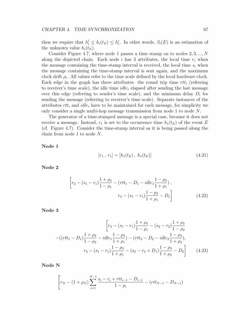
CHAPTER 4. TIME SYNCHRONIZATION 87
then we require that hli ≤ hi(tE) ≤ hr
i . In other words, Si(E) is an estimation ofthe unknown value hi(tE).
Consider Figure 4.7, where node 1 passes a time stamp on to nodes 2, 3, ..., Nalong the depicted chain. Each node i has 3 attributes, the local time ri whenthe message containing the time-stamp interval is received, the local time si whenthe message containing the time-stamp interval is sent again, and the maximumclock drift ρi. All values refer to the time scale defined by the local hardware clock.Each edge in the graph has three attributes: the round trip time rtti (referringto receiver’s time scale), the idle time idlei elapsed after sending the last messageover this edge (referring to sender’s time scale), and the minimum delay Di forsending the message (referring to receiver’s time scale). Separate instances of theattributes rtti and idlei have to be maintained for each message, for simplicity weonly consider a single multi-hop message transmission from node 1 to node N .
The generator of a time-stamped message is a special case, because it does notreceive a message. Instead, r1 is set to the occurrence time h1(tE) of the event E(cf. Figure 4.7). Consider the time-stamp interval as it is being passed along thechain from node 1 to node N .
Node 1
[r1 , r1] = [h1(tE) , h1(tE)] (4.21)
Node 2 [r2 − (s1 − r1)
1 + ρ2
1− ρ1
− (rtt1 −D1 − idle11− ρ2
1 + ρ1
) ,
r2 − (s1 − r1)1− ρ2
1 + ρ1
−D1
](4.22)
Node 3 [r3 − (s1 − r1)
1 + ρ3
1− ρ1
− (s2 − r2)1 + ρ3
1− ρ2
−((rtt1 −D1)1 + ρ3
1− ρ2
− idle11− ρ3
1 + ρ1
)− (rtt2 −D2 − idle21− ρ3
1 + ρ2
),
r3 − (s1 − r1)1− ρ3
1 + ρ1
− (s2 − r2 + D1)1− ρ3
1 + ρ2
−D2
](4.23)
Node N[rN − (1 + ρN)
N−1∑i=1
si − ri + rtti−1 −Di−1
1− ρi
− (rttN−1 −DN−1)

CHAPTER 4. TIME SYNCHRONIZATION 88
+(1− ρN)N−1∑i=1
idlei
1 + ρi
,
rN − (1− ρN)N−1∑i=1
si − ri + Di−1
1 + ρi
−DN−1
](4.24)
The interval for node 1 consists of the single point h1(tE). For node 2 the amount oftime s1− r1 (during which the message was stored in node 1 after being generatedand before being sent) is subtracted from the message arrival time r2. The differencertt1 − idle1 between round trip and idle time is used as an upper bound for themessage delay, the minimum delay D1 is used as a lower bound. Transforming timeintervals between the different time scales as described in Section 4.4.3 results inthe interval shown for node 2. Continuing this way with subtracting total nodestorage time from message arrival time and using the sum of round trip minus idletimes as the upper bound for message delay, and assuming rtt0 = 0 and D0 = 0,one will end up with the interval shown for node N .
4.4.6 Interval Arithmetic
Using the algorithm described in the previous sections, we are now able to decidetemporal predicates over time stamps using a variant of the interval arithmeticdescribed in [2]. To decide whether [hl
1, hr1] happened before [hl
2, hr2], for example,
the following rule can be used:
[hl1, h
r1] < [hl
2, hr2] =
YES : hr
1 < hl2
NO : hr2 < hl
1
MAYBE : otherwise(4.25)
To determine whether [hl1, h
r1] and [hl
2, hr2] happened within a certain real-time
interval T , the following rule is used:
∣∣[hl1, h
r1]− [hl
2, hr2]
∣∣ < T =YES : max(hr
2, hr1)−min(hl
2, hl1) < T (1− ρmax)
NO : max(hl2, h
l1)−min(hr
2, hr1) ≥ T (1 + ρmax)
MAYBE : otherwise(4.26)
Note that the real-time interval T has to be transformed to local time first bymultiplying with 1 ± ρmax, since all time-stamp intervals refer to the time scaledefined by the local hardware clock.
The real-time “distance” between two time-stamp intervals can be estimatedusing the following formula:∣∣[hl
1, hr1]− [hl
2, hr2]
∣∣ ≤ (max(hr2, h
r1)−min(hl
2, hl1))/(1− ρmax) (4.27)

CHAPTER 4. TIME SYNCHRONIZATION 89
Again, the calculated local time difference has to be transformed to real-time bydividing by 1− ρmax.
When comparing points in time (for example a locally generated h(tx)) withtime-stamp intervals received from other nodes, h(tx) can be treated as a time-stamp interval [h(tx), h(tx)] and used with the above equations.
4.4.7 Implementation
The basic idea for implementing the algorithm is to incrementally calculate thethree sums in the Formula 4.24 along the message path. The implementationassumes an asynchronous, reliable communication mechanism but can easily beextended to unreliable communication mechanisms (e.g., by means of timeoutsand retransmissions).
A time stamp can be represented in the following way using C:
struct TimeStamp {
Time begin, end, received;
Time s1, s2, s3;
};
where begin and end are the left and right ends of the time-stamp interval,received is the time of arrival, and where s1, s2, s3 are the three sums in For-mula 4.24 from left to right, which are incrementally calculated as the messageis forwarded from node to node. Note that begin, end, and received are localvariables that don’t need to be transmitted between nodes. One or more instancesof TimeStamp can be contained in an application message.
Time is a representation for points in time and time differences. Computerclocks are discrete, so an integer type would be appropriate. But care has to betaken because of time transformations, which may result in fractional values, soeither a floating-point type must be used or the results have to be rounded suchthat the integer interval always contains the floating-point interval. Here we assumefloating point values.
The generator of a time-stamped message performs the following actions:
1 Generator:
2 TimeStamp S;
3 S.begin = S.end = S.received = NOW;
4 S.s1 = S.s2 = s3 = 0;
where NOW refers to the current value of the local clock. As explained in the previoussection, the interval is initialized to current time in the node. All other fields areset to zero.
A time-stamped message is sent using the following actions:
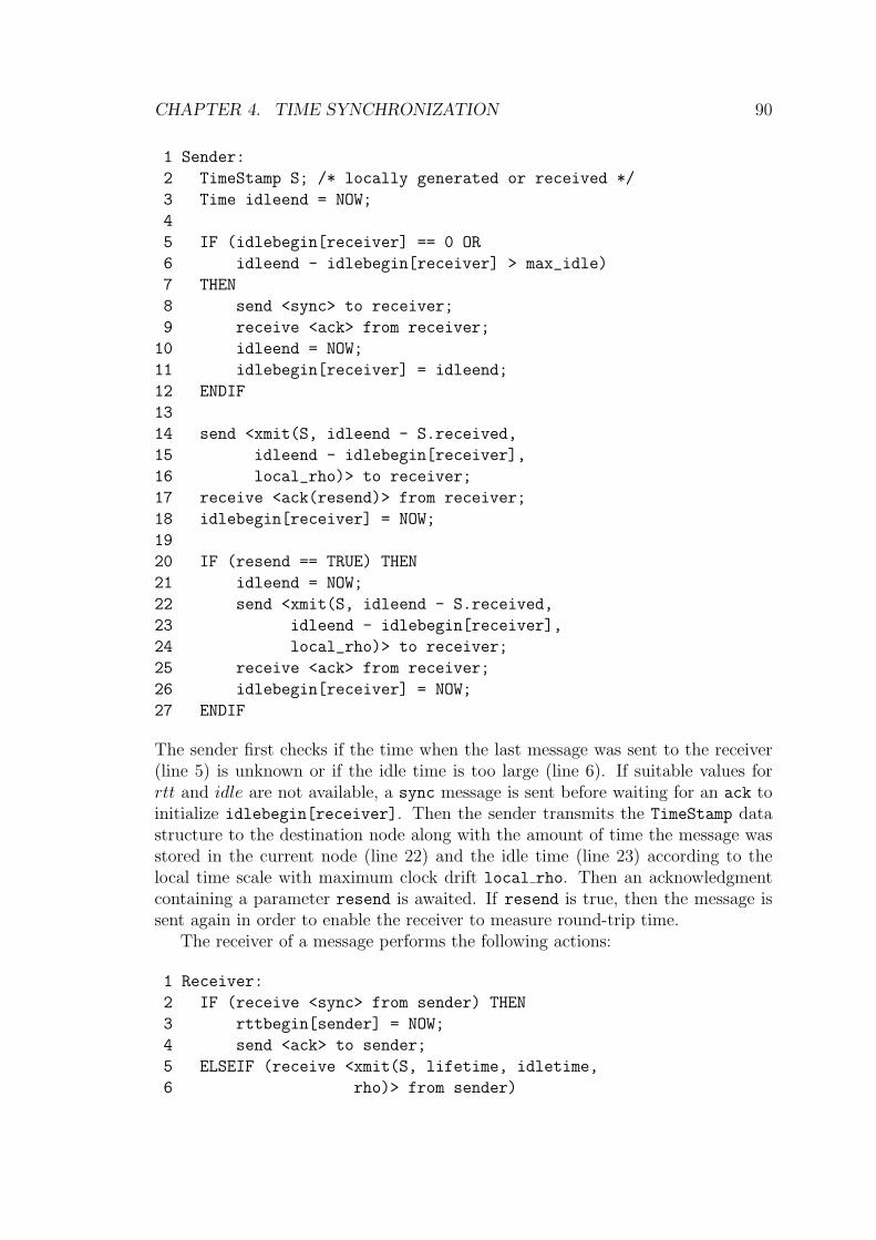
CHAPTER 4. TIME SYNCHRONIZATION 90
1 Sender:
2 TimeStamp S; /* locally generated or received */
3 Time idleend = NOW;
4
5 IF (idlebegin[receiver] == 0 OR
6 idleend - idlebegin[receiver] > max_idle)
7 THEN
8 send <sync> to receiver;
9 receive <ack> from receiver;
10 idleend = NOW;
11 idlebegin[receiver] = idleend;
12 ENDIF
13
14 send <xmit(S, idleend - S.received,
15 idleend - idlebegin[receiver],
16 local_rho)> to receiver;
17 receive <ack(resend)> from receiver;
18 idlebegin[receiver] = NOW;
19
20 IF (resend == TRUE) THEN
21 idleend = NOW;
22 send <xmit(S, idleend - S.received,
23 idleend - idlebegin[receiver],
24 local_rho)> to receiver;
25 receive <ack> from receiver;
26 idlebegin[receiver] = NOW;
27 ENDIF
The sender first checks if the time when the last message was sent to the receiver(line 5) is unknown or if the idle time is too large (line 6). If suitable values forrtt and idle are not available, a sync message is sent before waiting for an ack toinitialize idlebegin[receiver]. Then the sender transmits the TimeStamp datastructure to the destination node along with the amount of time the message wasstored in the current node (line 22) and the idle time (line 23) according to thelocal time scale with maximum clock drift local rho. Then an acknowledgmentcontaining a parameter resend is awaited. If resend is true, then the message issent again in order to enable the receiver to measure round-trip time.
The receiver of a message performs the following actions:
1 Receiver:
2 IF (receive <sync> from sender) THEN
3 rttbegin[sender] = NOW;
4 send <ack> to sender;
5 ELSEIF (receive <xmit(S, lifetime, idletime,
6 rho)> from sender)

CHAPTER 4. TIME SYNCHRONIZATION 91
7 THEN
8 Time rttend = NOW;
9 IF (rttbegin[sender] == 0) THEN
10 rttbegin[sender] = NOW;
11 send <ack(TRUE)> to sender;
12 ELSE
13 S.s1 += lifetime/(1 - rho);
14 S.s2 += idletime/(1 + rho);
15 S.s3 += lifetime/(1 + rho);
16 S.begin = rttend
17 - S.s1*(1 + local_rho)
18 + S.s2*(1 - local_rho)
19 - (rttend - rttbegin[sender]) + D;
20 S.end = rttend
21 - S.s3*(1 - local_rho)
22 - D;
23 M.s1 += (rttend - rttbegin[sender] - D)
24 * (1 - local_rho);
25 M.s3 += D*(1 + local_rho);
26 rttbegin[sender] = NOW;
27 send <ack(FALSE)> to sender;
28 ENDIF
29 ENDIF
The receiver waits for a sync or xmit message from a sender. If it receives a sync,it just initializes rttbegin[sender] and returns an ack to the sender.
If an xmit message is received, then the receiver first checks if the time ofarrival of a previous message from this sender is known (line 9). If not so, thenrttbegin[sender] is initialized and an ack(TRUE) message is returned to thesender, asking for a retransmission.
If rttbegin[sender] is known in the sender, then the fields of the receivedtime stamp S are updated according to Equation 4.24 and S.begin and S.end
are calculated. Note that the received value for S.s1 (S.s3) does not yet includethe last rtt and D values, so it has to be explicitly subtracted in lines 19 and 22without time transformation, since rtt and D have been measured with respect toreceiver’s time scale. Only after S.begin and S.end have been calculated, M.s1(M.s3) are updated accordingly. Finally, an ack is sent back to the sender.
The checks for idlebegin[receiver] and rttbegin[sender] in sender andreceiver, respectively, enable both the sender and receiver to independently dropentries from the sets idlebegin and rttbegin in order to limit the memory foot-print as described in Section 4.4.4.

CHAPTER 4. TIME SYNCHRONIZATION 92
4.4.8 Evaluation
In this section we examine the compliance of TSS with the region in the designspace indicated in Section 4.3.
Intermittent Connectivity
If a message can be forwarded from a source node to a destination node (possiblyacross temporary partition boundaries), synchronization can be performed as well,provided that connections between adjacent nodes remain established long enoughfor at most two round-trip message exchanges.
Resource Efficiency
In most cases, TSS can piggyback on existing network traffic, resulting in a slightincrease of the size of messages that carry a time stamp. With the implementationin Section 4.4.7, every message would contain the partial sums s1, s2, s3, lifetime,idletime, and local rho. Assuming sizeof(Time) = 4 and sizeof(local rho)
= 1, the size of a message would increase by 17 bytes compared to a simple time-stamp of type Time. Note that local rho could be cached by the receiver. Itmight also be worthwhile to use a variable bit-length encoding for the various Timevalues, since lifetime and idletime (but also the partial sums) tend to be smallin unpartitioned networks.
Additional messages are only needed when a pair of nodes first communicates orwhen two nodes haven’t communicated for a long time. Hence, additional overheadis only introduced when a pair of nodes has been “idle” before. Under “heavy load”,when a pair of nodes communicates frequently, no additional messages are required.
Correctness
Since time-stamps are represented as intervals in TSS, temporal predicates canalways be decided correctly or not at all according to the rules in Section 4.4.6.
Precision
In order to get an impression of the precision of the algorithm TSS we performedsome measurements on a cluster of 800 MHz Pentium III Linux PCs connected by100 Mbit/s Ethernet using TCP and assuming ρ = 10−6. This has to be consideredas a best case scenario, since sensor networks typically use a networking technologyproviding a bandwidth well below 1 Mbit/s and embedded processors with no morethan 10 MIPS. However, since the algorithm is neither especially CPU intensivenor network-bandwidth intensive, the measurements should give a good impressionof the algorithm’s possible precision.
Synchronization inaccuracies show up as time-stamp intervals of increasinglength and stem from two different sources. Firstly, due to the clock drift, in-terval length increases with the age of a time stamp. Secondly, the interval length

CHAPTER 4. TIME SYNCHRONIZATION 93
0 100 200 300 400 500 600 700 800 9000
500
1000
1500
2000
2500
3000
3500
4000
Age [s]
Inte
rval
leng
th [u
s]
Figure 4.8: Precision depending on age.
increases with the number of hops a time stamp has been passed along, due to theestimation of messages delays.
We performed two measurements, the first of which examines time-stamp in-terval length as a function of time-stamp age. Since the error resulting from age isadditive over the nodes, we generate a zero-length time stamp interval in node 1,store it for X seconds before forwarding it to node 2, which prints out the lengthof the received time-stamp interval. We repeat this experiment 1000 times andcalculate averages. Figure 4.8 shows the results1, indicating a linear increase ofimprecision with age.
The second measurement examines time-stamp interval length as a function ofthe number of hops a time stamp has been passed along. We generate a zero-lengthtime-stamp interval in node 1 and pass it on to node 2, 3, ..., 7, which all print outthe length of the received time-stamp interval. We repeat this experiment 1000times and calculate averages. Figure 4.9 shows the results2, indicating a linearincrease of inaccuracy with the number of hops.
Since the two types of inaccuracies are additive, one can interpret the measure-ments as follows: Passing a time stamp along no more than 5 hops with an ageof no more than 500 seconds, one can expect an inaccuracy of no more than 3msin the examined setting. That is, exact results (as opposed to MAYBE) can beobtained as long as compared time stamps represent points in time which are more
1The exact interval lengths are 195, 585, 982, 1378, 1775, 2170, 2609, 2992, 3369, 3764µs.2The exact interval lengths are 0, 201, 400, 562, 752, 926, 1113, 1273µs.

CHAPTER 4. TIME SYNCHRONIZATION 94
0 1 2 3 4 5 6 70
200
400
600
800
1000
1200
1400
Number of hops
Inte
rval
leng
th [u
s]
Figure 4.9: Precision depending on number of hops.
than 6ms apart, since then the time-stamp intervals (3ms each) cannot overlap.With less than 6ms difference, an exact answer may still be obtained, but MAYBEresults are likely.
These measurements indicate that “collocated events” (both in time and space)can be synchronized with good precision. The larger the distance between theevents in time and space, the lower is the precision.
4.4.9 Potential Improvements
There are several potential approaches to improve the accuracy of the algorithm(i.e., reduce the probability of MAYBE results), which might be worth furtherinvestigation. In general, these techniques tend to improve precision by introducingadditional overheads.
One idea to avoid MAYBE results when comparing time stamps originatingfrom the same node is to keep a history of time stamps instead of only one timestamp. Instead of updating a time stamp upon receipt, the receiving node appendsthe updated time stamp together with a unique node identifier i and ρi to thetime stamp history or reuses a time stamp from the history if there is an entryfor node i in the history already. If comparing time stamps results in MAYBE,then the histories of the compared stamps are searched for common nodes and thecomparison is repeated using the time stamps of these common nodes, transformingtime values if necessary, and using the according ρ values from the histories. Thisis likely to give a “better” (i.e., non-MAYBE) answer, since imprecision increases

CHAPTER 4. TIME SYNCHRONIZATION 95
S
S
1
2
h
h
h
h
1 1r
2l
2
l
r
Figure 4.10: Overlapping time stamp intervals.
with age and hop count of the time stamps. For the same reason the accuracy ofcalculated real-time spans can be improved by using “younger” time stamps fromthe history in the same way whenever possible.
A different and more general approach is to replace MAYBE results with aprobability depending on the relative arrangement of the compared time-stampintervals. The algorithm would then output “X < Y with probability p” insteadof “Xmaybe < Y ”. To implement this, we have to derive probability distributionsfor the exact time instants over the time-stamp intervals.
Consider for example the two overlapping time-stamp intervals S1 and S2 withhl
1 ≤ hl2 ≤ hr
1 ≤ hr2 shown in Figure 4.10, for which the algorithm would output
“S1maybe < S2”. If we knew probability distributions p1(h) and p2(h), such thatpi(hi) is the probability that the exact point in time represented by Si is hi, wecould calculate the probability p for S1 < S2 by “iterating” over the possible h1
values and summing up the probabilities for h1 < h2:∫ hr1
hl1
p1(h1)
(∫ tr2
t
p2(h2)dh2
)dh1 (4.28)
For uniform distributions pi(h)3 this evaluates to
hl2 − hl
1
hr1 − hl
1
+hr
2(hr1 − hl
2)− (hr12 − hl
22)/2
(hr1 − hl
1)(hr2 − hl
2)(4.29)
Assuming, for example, hl1 = 0, hr
1 = hr2 = 2, and hl
2 = 1, we can calculatethe probability for S1 < S2 as 0.75. Assuming a uniform distribution, however,usually is an oversimplification, since due to the characteristics of the algorithm4
the probability in the middle of the interval is much higher than at the ends. Itremains an open task to obtain good probability distributions. Furthermore ithas to be investigated for which cases knowing a probability instead of MAYBE isadvantageous for applications.
3p1(h) = 1/(hr1 − hl
1) for h ∈ [hl1, h
r1] and 0 otherwise; p2(t) likewise.
4We use D and rtt as lower and upper bounds for the message delay. It is much more likelythat the actual message delay is about rtt/2 than D or rtt.

CHAPTER 4. TIME SYNCHRONIZATION 96
4.5 Summary
This chapter is devoted to time synchronization in wireless sensor networks. Wefirst discussed important models with respect to hardware clocks and communica-tion. Following the framework developed in Chapter 3, we then presented impor-tant concepts used by time synchronization algorithms. Referring to these concepts,we then presented and discussed important existing approaches to time synchro-nization – both in traditional distributed systems and for sensor networks. Wethen identified a region in the design space that cannot be appropriately supportedby these existing algorithms. In particular, we showed that networks with inter-mittent connectivity are not sufficiently supported. We presented and evaluatedTime-Stamp Synchronization to support this region in the design space. A keyfeature of Time-Stamp Synchronization is that rather than synchronizing clocks,time stamps are transformed between the unsynchronized time-scales of sensornodes. We showed that this approach is efficient since time information can bepiggybacked on existing message exchanges. Based on a prototypical implementa-tion, we evaluated the precision of our approach and found that imprecision growslinearly with the age of time stamps and with the hop-distance between nodes,providing an accuracy in the order of milliseconds. Finally, we discussed potentialimprovements in settings where precision is more important than efficiency.

Chapter 5
Sensor Node Localization
The significance of physical space for sensor networks has been reflected by thedevelopment of a number of node localization algorithms in the recent past. How-ever, most of these approaches have been designed for “traditional” sensor net-works, covering only a small region of the design space discussed in Section 2.2.We will identify an important region in the design space that is not sufficientlysupported by existing algorithms. In order to fill this gap, we present and evaluatean approach called “Lighthouse Location System”.
We begin our discussion in Section 5.1 by studying fundamental system modelsand by presenting concrete algorithmic techniques for localization. The discussionwill be structured according to the common framework we developed in Chapter 3.Referring to these techniques, we present existing algorithms for node localizationin Section 5.2. Our algorithm will be motivated and presented in Sections 5.3 and5.4.
5.1 Background
This section reviews models and concepts for node localization. The discussion isstructured according to Section 3.3.
5.1.1 Signal Propagation and Mobility Models
In the following two subsections we discuss models of signal propagation and ofnode mobility. The propagation of signals such as radio or sound are fundamentalfor measuring spatial relationships among nodes. Models of node mobility can helpmaintain localization over time.
Signal Propagation Models
Many localization approaches for sensor networks assume that sensor nodes areequipped with hardware for measuring spatial relationships among nodes such as
97

CHAPTER 5. SENSOR NODE LOCALIZATION 98
distance or direction. For this purpose, some systems reuse existing radios orig-inally intended for data communication, others introduce additional sensors andactuators to achieve a satisfactory precision. Besides radio, audio is perhaps themost commonly used signal modality for this purpose.
Two signal propagation features commonly used for measuring spatial relation-ships are propagation delay and received signal strength, since both are functions ofthe distance between emitter and receiver of a signal. Deriving spatial relationshipsfrom a measured propagation delay requires a precise model of the propagationspeed of the signal. The derivation of spatial relationships from received signalstrength requires a precise model of signal attenuation.
Signal propagation speed is mainly a function of the signal modality, its fre-quency, and of the medium. For example, the propagation speed of radio wavescan diverge significantly from c in vacuum and air. In water (and wet materials),for example, propagation speed is about c/1.33. The radio propagation speed isalso influenced by ionizing radiation (e.g., solar winds), where the speed reductiondepends on the frequency of the signal. With acoustic waves, the propagationspeed varies between about 60m/s (e.g., rubber) and about 6000m/s (e.g., stone).In air, propagation speed depends on factors such as temperature, and – to a lesserextent – humidity and pressure. For example, propagation speed in air at -20◦C is320m/s, whereas 344m/s are found for +20◦C. A more precise model for speed ofsound in air is:
cair =√
γRT (5.1)
where T is absolute temperature, R is the gas constant (286 m2/s2/K), and whereγ is the heat capacity ratio (about 1.4 for typical humidity and pressure values).The effective speed of sound also depends on movements of the medium such aswinds and convection streams.
Typical localization systems use one out of the following three approaches tomodel propagation speed. Firstly, a constant speed is assumed that may be cali-brated under operating conditions using separate calibration equipment. Secondly,additional sensors may be attached to nodes in order to measure parameters thatinfluence the propagation speed (e.g., temperature for speed of sound). Thirdly,the propagation speed is treated as an unknown variable in addition to the soughtlocation. Additional constraints are required in order to solve for propagation speedand location.
The received signal strength depends on the emitted signal strength and theattenuation. Attenuation is a function of the signal modality, frequency, and themedium. In general, an omni-directional source radiating into free space can bemodeled as
P = kPs/re (5.2)
where e = 2, Ps is the emitted power, r is the distance between sender and receiver,and k is a constant factor. The quadratic relationship stems from the fact thatthe emitted power is equally spread over the points on a sphere with radius r.

CHAPTER 5. SENSOR NODE LOCALIZATION 99
In physical structures where signal propagation is limited to certain regions (e.g.,corridors), smaller attenuation exponents between 1.5 and 2 may be observed.
Additional sources of attenuation are absorption of the medium, interactionof the signal with reflective surfaces, and interaction of the signal with obstaclesbetween emitter and receiver. Radio waves, for example, are absorbed by ionizedgases. Sound waves are absorbed in gases due to friction between molecules thatresults in heat generation. Reflective surfaces may lead to the situation that areflected signal interferes with the unreflected (or another reflected) signal at thereceiver. This can be observed, for example, if emitter and receiver are near theground or if the environment is cluttered with reflective surfaces. Radio waves oftenexperience a phase shift close to 180◦ when reflected, which often leads to destruc-tive interference. Hence, for near-ground radio communication the exponent e inEquation 5.2 is close to 4. In highly cluttered environments with many reflectionsinterfering at the receiver, e may be as large as 6. Sound waves are less susceptibleto such interference effects, since the above mentioned phase shift is typically notfound. For near-ground communication, for example, e is still close to 2.
Additional sources of attenuation for sound in air are meteorological conditionssuch as wind-velocity gradients (e.g., due to friction with the ground) and tem-perature gradients (e.g., due to heat disseminated by the ground). Both resultin gradients in sound velocity which lead to a refraction effect, such that soundwaves are bent upwards or downwards with respect to the ground, depending onthe relative direction of the waves to the gradient. One further source of attenua-tion of sound in air are random fluctuations of wind and temperature which causefluctuations in amplitude and phase of the signal at the receiver.
The above discussion should make it obvious that models for signal attenuationdo heavily depend on the environment where they are used in. Note that evensmall changes in the locations of emitter, receiver, or reflective surfaces may causesignificant changes in received signal strength due to changed conditions for multi-path interference. This is particularly relevant for radio waves, where multi-pathinterference can have a significant impact on the attenuation exponent in Equation5.2. Hence, large errors must be expected if the model does not correctly representreality. Typical models used in localization systems are based on Equation 5.2 withe = 4. Range measurement errors based on such models can be in the order of 40%and above [88].
The use of signal propagation features for range measurements obviously re-quires that the signal can travel along the line-of-sight path between the emitterand the receiver. If the direct line is blocked by non-transparent obstacles, thesignal may reach the receiver due to reflections. Since the effective length of suchreflected paths is longer than the line of sight, the resulting distance estimates willbe greater than the Euclidean distance.
Many of the above signal propagation properties depend on the actual frequencyof the signal. Hence, the use of wide-band signals (which contain many differentfrequencies) can help mitigate or compensate errors that are due to frequency-dependent propagation properties. Also, wide-band techniques are robust to in-

CHAPTER 5. SENSOR NODE LOCALIZATION 100
terference with narrow-band signals emitted by other sources in range (e.g., mi-crowave ovens, acoustic background noise) [42, 43]. Likewise, the use of differentsignal modalities (e.g., sound and radio) can help improve robustness and precision(cf. Section 2.7.2).
Mobility Models
Mobility models are mechanism to describe possible movements and locations ofmobile entities. They can be a valuable tool for improving the precision of localiza-tion approaches since they provide hints on the possible locations of a sensor node.Two very simple mobility models are the “static model” where nodes do not moveat all and the “unconstrained mobility model” where nodes can be at any placeanytime. Between these two extremal models, a number of more realistic modelscan be found.
Basically, a mobility model imposes constraints on the possible location, speed,and acceleration of a mobile entity. These constraints can be either static or dy-namic. In static models, the same constraints apply always. In dynamic models,the constraints may be a function of time or of previous system states. If, for ex-ample, a sensor node is attached to a car, possible node locations are constrainedto roads (with high probability), there are bounds on the speed and accelerationof the sensor node. While these constraints are static, we can also identify dy-namic constraints, where future locations of the sensor node are constrained byits previous locations. For example, a car is very unlikely to leave a crossing viathe same road it entered. Given such a set of constraints, the location of the nodeat some time t0 (and possibly also earlier locations of the node), we can derivea set of possible locations of the node at some time t1 > t0 without making anymeasurements.
A number of mobility models are commonly used to study the behavior of mo-bile systems, for example the random waypoint model (a node chooses a randomdestination point and moves there on a straight line with constant speed, stops forsome time before choosing a new destination). Another common class of mobilitymodels are graph-based, where a node can only move along the edges of an Eu-clidean graph. At each vertex, one of the outgoing edges is chosen according tospecific rules (e.g., random walks).
5.1.2 Obtaining Constraints
There are two basic types of spatial relationships that are used as constraints forlocalization: distances and angles.
Distance Constraints
Distances are used in two variants: absolute distance to a reference node anddistance differences to two or more reference nodes. Absolute distances can beobtained by measuring time-of-flight or received signal strength, using propagation

CHAPTER 5. SENSOR NODE LOCALIZATION 101
(c)(a) (b) (d) (e) (f)
Figure 5.1: References (black) impose constraints (red regions) on the locationsof a client node (white). (a) Distance estimate, (b) distance bound, (c) distancedifference, (d) closest reference, (e) direction of arrival estimate, and (f) directionof arrival bounds.
models as described in Section 5.1.1. Note that time-of-flight measurements requiresome form of time synchronization between sender and receiver. The precision ofsynchronized time is determined by the precision that is required for the distanceestimate. For received signal strength, the emitted signal strength must also beknown. The resulting distance constraint is illustrated in Figure 5.1 (a).
While the above approach typically results in point estimates for distance, thereis also a notable method for obtaining bounds based on network connectivity. Ifthe communication range of a sensor node is at most R, then two nodes that canhear each other are at most R apart. The resulting constraint is illustrated inFigure 5.1 (b). In some cases it is preferable to use a bounding box instead of adistance constraint as indicated by the dashed rectangle in (b). For example, theintersection of two bounding boxes is also a bounding box, while the intersectionof two spheres is not a sphere anymore.
Distances and distance bounds can also be combined across multiple hops toobtain distance bounds for client nodes that are not network neighbors of a refer-ence node. If two nodes are separated by N hops, their distance is at most NR.Similarly, if the distances along a path between two nodes are r1, ..., rN , than thedistance between the nodes is at most
∑ri.
Distance differences can be obtained by measuring the time difference(s) be-tween the arrival of signals emitted by two or more synchronized reference nodes,or by measuring the differences between the received strengths of signals emittedby two or more reference nodes with identical emitted signal strengths. Distance-difference estimates can then be obtained by applying the propagation models tothe time or signal strength differences. Note that the resulting constraint theninvolves multiple reference nodes as exemplified in Figure 5.1 (c). Figure (d) il-lustrates a bound-based variant of distance differences, where a node determinesto which of a set of references it is closest (i.e., reference with strongest receivedsignal or reference with earliest time of arrival).

CHAPTER 5. SENSOR NODE LOCALIZATION 102
Angular Constraints
Angles are mainly used in form of direction of arrival. If a node is located at theorigin of a 2D coordinate system, then the direction of arrival can be modeledas the angle enclosed between the x axis and a line connecting origin with thereference node. In order to measure direction of arrival, complex hardware istypically required. One possible approach are sector antennas, where multipledirectional antennas are arranged such that each possible sender can be receivedby at least one antenna. Since each antenna has a well-defined angle of beamspread, bounds on the angle of incidence can be obtained. As illustrated in Figure5.1 (f), this results in a constraint on the location of the node. Another approach isthe use of multiple omnidirectional receivers with known baselines in between. Bymeasuring the time difference of arrival at these receivers, the direction of arrivalcan be estimated, which results in a constraint on the node location as illustratedin Figure 5.1 (e).
Note that it is also possible to combine angular and distance measurements.However, due to the hardware overhead, increased size and cost of sensor nodes,angle-based approaches are barely used for sensor networks.
5.1.3 Combining Constraints
A single constraint can be interpreted as a set of possible node locations that typ-ically form a connected region in space as illustrated in Figure 5.1. Combiningmultiple constraints is then equivalent to computing the intersection of the respec-tive regions. In some cases the exact shape of the intersection region is required,sometimes a single point that lies in the intersected region is computed, and insome cases a simple shape (e.g., bounding box or sphere) that is enclosed by orenclosed the intersection region is sought.
Typically an intersection is derived analytically, but there are situations wherethis is infeasible or undesirable due to computational overheads. A notable alter-native is to partition space into pixels or voxels (i.e., 3D pixels), such that the edgelength of a pixel equals the required precision. A single bit is associated with eachpixel, which is initially set to “1”. For each available constraint, the pixels thatare outside the region represented by the constraint are set to “0”. Eventually, theremaining “1” pixels form an approximation of the intersection region.
Due to measurement errors it may occur that a given set of constraints has anempty intersection. There are basically two approaches to deal with such cases.Firstly, outliers can be rejected, such that a set of constraints with a non-emptyintersection is obtained. As for time synchronization, various criteria can be ap-plied to control selection of these constrains (e.g., minimize number of rejectedconstraints, minimize intersection region). Secondly, a solution (typically a singlepoint) can be computed that minimizes a certain error metric. For example, theerror of a point solution with respect to a single constraint can be defined as thesmallest distance between the solution point and any point contained in the regiondefined by the constraint. The sought solution should then minimize the sum of
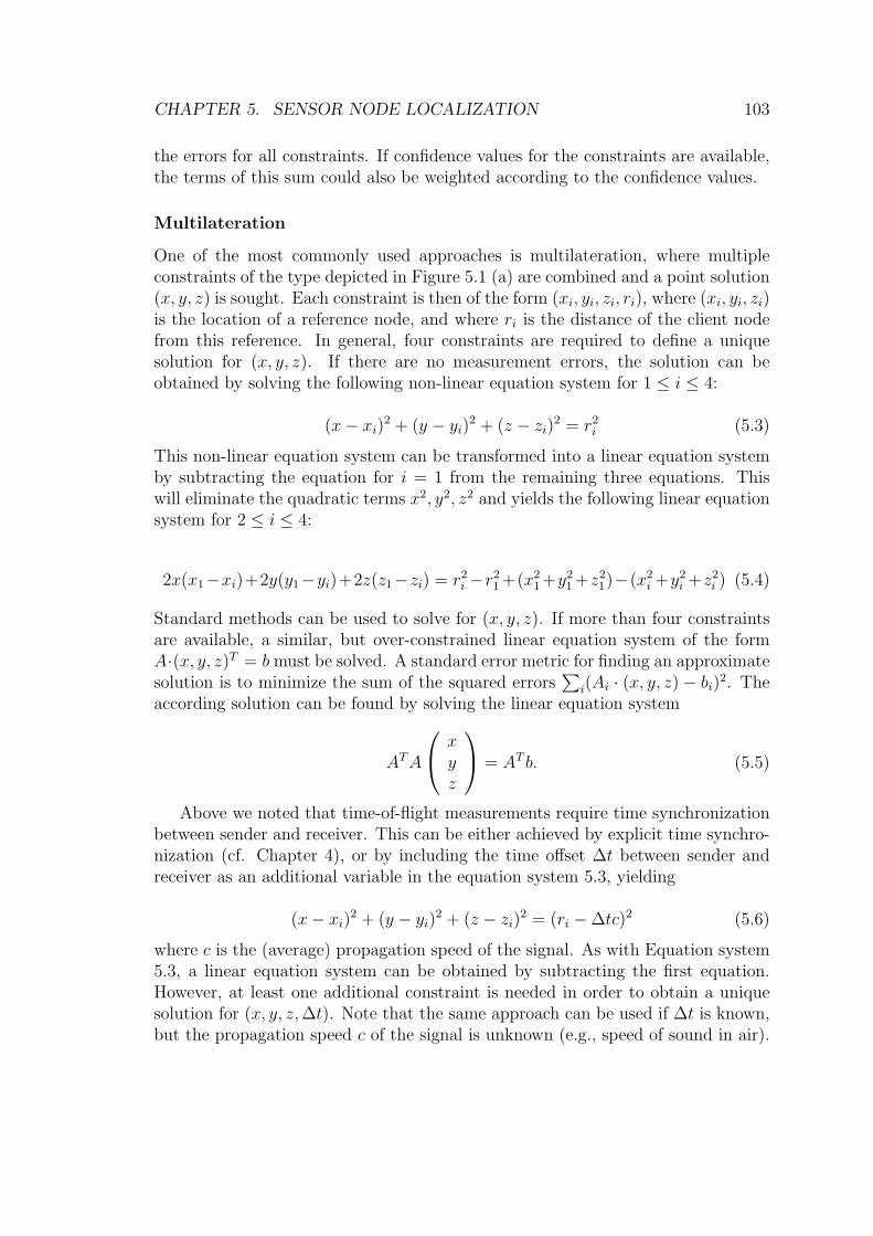
CHAPTER 5. SENSOR NODE LOCALIZATION 103
the errors for all constraints. If confidence values for the constraints are available,the terms of this sum could also be weighted according to the confidence values.
Multilateration
One of the most commonly used approaches is multilateration, where multipleconstraints of the type depicted in Figure 5.1 (a) are combined and a point solution(x, y, z) is sought. Each constraint is then of the form (xi, yi, zi, ri), where (xi, yi, zi)is the location of a reference node, and where ri is the distance of the client nodefrom this reference. In general, four constraints are required to define a uniquesolution for (x, y, z). If there are no measurement errors, the solution can beobtained by solving the following non-linear equation system for 1 ≤ i ≤ 4:
(x− xi)2 + (y − yi)
2 + (z − zi)2 = r2
i (5.3)
This non-linear equation system can be transformed into a linear equation systemby subtracting the equation for i = 1 from the remaining three equations. Thiswill eliminate the quadratic terms x2, y2, z2 and yields the following linear equationsystem for 2 ≤ i ≤ 4:
2x(x1−xi)+2y(y1−yi)+2z(z1−zi) = r2i −r2
1 +(x21 +y2
1 +z21)−(x2
i +y2i +z2
i ) (5.4)
Standard methods can be used to solve for (x, y, z). If more than four constraintsare available, a similar, but over-constrained linear equation system of the formA·(x, y, z)T = b must be solved. A standard error metric for finding an approximatesolution is to minimize the sum of the squared errors
∑i(Ai · (x, y, z) − bi)
2. Theaccording solution can be found by solving the linear equation system
AT A
xyz
= AT b. (5.5)
Above we noted that time-of-flight measurements require time synchronizationbetween sender and receiver. This can be either achieved by explicit time synchro-nization (cf. Chapter 4), or by including the time offset ∆t between sender andreceiver as an additional variable in the equation system 5.3, yielding
(x− xi)2 + (y − yi)
2 + (z − zi)2 = (ri −∆tc)2 (5.6)
where c is the (average) propagation speed of the signal. As with Equation system5.3, a linear equation system can be obtained by subtracting the first equation.However, at least one additional constraint is needed in order to obtain a uniquesolution for (x, y, z, ∆t). Note that the same approach can be used if ∆t is known,but the propagation speed c of the signal is unknown (e.g., speed of sound in air).

CHAPTER 5. SENSOR NODE LOCALIZATION 104
Figure 5.2: Four references with known locations define unique locations for twonodes if distances between connected nodes are known. Traditional multilaterationcannot be applied, since there are too few constraints for each individual node.
Collaborative Multilateration
In some node constellations too few constraints may be available to obtain a uniquesolution for (x, y, z). However, by including other nodes with unknown locationsinto consideration, a unique solution can often be found anyway. As depicted inFigure 5.2, four black reference nodes define unique locations for two client nodesif the distances between connected nodes are known. Obtaining a solution for thelocations of two or more client nodes in such situations is referred to as collaborativemultilateration. One possible approach to find a solution for such problems is torequest that a measured distance rij between nodes i and j should be matchedby the distance
√(xi − xj)2 + (yi − yj)2 + (zi − zj)2 between the sought location
estimates (xi, yi, zi) and (xj, yj, zj) for nodes i and j. An optimization problem canbe formulated by minimizing the sum of the squared errors over all edges (i, j):
min∑(i,j)
(rij −
√(xi − xj)2 + (yi − yj)2 + (zi − zj)2
)2
(5.7)
The resulting non-linear optimization problem typically does not have a closed-formsolution and numerical approximations must be applied to find the solution.
Centroids
This approach considers the problem of finding a point in the intersection of anumber of distance-bound constraints (cf. Figure 5.1 (b)) for a single node. Sucha point can be obtained by computing the average (i.e., centroid) of the locationsof all references that define constraints on the node.
Triangle Test
This approach uses distance-difference constraints (cf. Figure 5.1 (d)) to decidewhether a node is contained in a triangle formed by three reference nodes withknown locations. This test is based on the following property: a node locatedoutside the triangle can be moved, such that the distances to all references areeither all increased or all decreased simultaneously. In contrast, all movements ofa node located inside the triangle will increase the distance to some references anddecrease the distance to other references simultaneously.
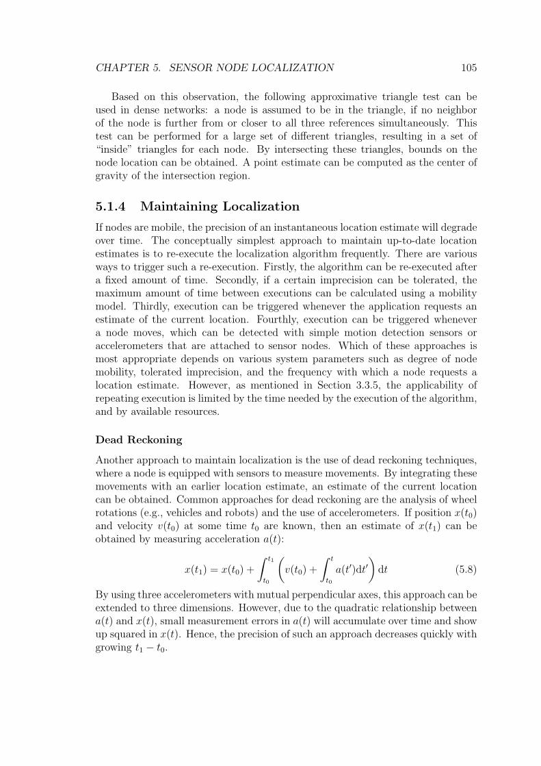
CHAPTER 5. SENSOR NODE LOCALIZATION 105
Based on this observation, the following approximative triangle test can beused in dense networks: a node is assumed to be in the triangle, if no neighborof the node is further from or closer to all three references simultaneously. Thistest can be performed for a large set of different triangles, resulting in a set of“inside” triangles for each node. By intersecting these triangles, bounds on thenode location can be obtained. A point estimate can be computed as the center ofgravity of the intersection region.
5.1.4 Maintaining Localization
If nodes are mobile, the precision of an instantaneous location estimate will degradeover time. The conceptually simplest approach to maintain up-to-date locationestimates is to re-execute the localization algorithm frequently. There are variousways to trigger such a re-execution. Firstly, the algorithm can be re-executed aftera fixed amount of time. Secondly, if a certain imprecision can be tolerated, themaximum amount of time between executions can be calculated using a mobilitymodel. Thirdly, execution can be triggered whenever the application requests anestimate of the current location. Fourthly, execution can be triggered whenevera node moves, which can be detected with simple motion detection sensors oraccelerometers that are attached to sensor nodes. Which of these approaches ismost appropriate depends on various system parameters such as degree of nodemobility, tolerated imprecision, and the frequency with which a node requests alocation estimate. However, as mentioned in Section 3.3.5, the applicability ofrepeating execution is limited by the time needed by the execution of the algorithm,and by available resources.
Dead Reckoning
Another approach to maintain localization is the use of dead reckoning techniques,where a node is equipped with sensors to measure movements. By integrating thesemovements with an earlier location estimate, an estimate of the current locationcan be obtained. Common approaches for dead reckoning are the analysis of wheelrotations (e.g., vehicles and robots) and the use of accelerometers. If position x(t0)and velocity v(t0) at some time t0 are known, then an estimate of x(t1) can beobtained by measuring acceleration a(t):
x(t1) = x(t0) +
∫ t1
t0
(v(t0) +
∫ t
t0
a(t′)dt′)
dt (5.8)
By using three accelerometers with mutual perpendicular axes, this approach can beextended to three dimensions. However, due to the quadratic relationship betweena(t) and x(t), small measurement errors in a(t) will accumulate over time and showup squared in x(t). Hence, the precision of such an approach decreases quickly withgrowing t1 − t0.

CHAPTER 5. SENSOR NODE LOCALIZATION 106
(a) (b)
Figure 5.3: Overlay topologies used by localization algorithms. (a) Stars, (b)clusters.
Prediction
Prediction based on mobility models is another approach to maintain localizationover time. Here, past locations of a node at time t ≤ t0 are used with a mobilitymodel to obtain constraints on the location of the node at time t1 > t0. Witha mobility model where velocity is limited by 0 ≤ v ≤ vmax, for example, thefollowing constraint can be derived:
x(t0) ≤ x(t1) ≤ x(t0) + vmax(t1 − t0) (5.9)
Note that depending on the used mobility model, the obtained constraints maybecome very loose with growing t1−t0. Overall, both dead reckoning and predictionare helpful approaches to bridge short gaps between consecutive executions of alocalization algorithm. While prediction and dead reckoning are very commonlyused for time synchronization (cf. Section 4.1.4), they are currently barely used forlocalization as far as the domain of sensor networks is concerned.
5.1.5 Selecting Constraints
Most localization algorithms are unstructured, that is, they use any available nodesin the neighborhood for obtaining constraints. The reason for this is that in orderto achieve a good precision, measurement errors must often be compensated by alarge number of constraints.
Two commonly used overlay topologies are depicted in Figure 5.3. With the startopology depicted in (a), nodes use all available references in their neighborhood toestimate their location, but nodes with estimated locations are not used as refer-ences for other nodes. In (b), nodes in a cluster establish a local coordinate systemand estimate their locations with respect to this reference grid. Adjacent clustersshare a number of nodes to allow for the derivation of a coordinate transformationbetween these clusters.
CHAPTER 5. SENSOR NODE LOCALIZATION 107
5.2 Related Work
This section presents and discusses existing approaches for node localization. Wefirst discuss related and influential approaches from other domains, pointing outtheir shortcomings in the context of sensor networks. Our main focus is, however,on algorithms which have been specifically developed for sensor networks. Theseare based on the models and concepts presented in the previous section.
5.2.1 Traditional Localization Approaches
In this section we consider two representative localization systems that have beendeveloped for applications other than sensor networks.
Global Positioning System
GPS [47] is based on 24 satellites orbiting the earth. All satellites broadcast signalsthat are used for time-of-flight measurements and which carry additional informa-tion such as current time and location of the satellites. The satellites are veryaccurately synchronized with each other. A GPS receiver uses a so-called almanacand the information transmitted by the satellites to maintain precise estimatesof the current locations and time of the satellites. The almanac is essentially a(mobility) model of the satellite orbits.
In order to obtain a location estimate, a GPS receiver measures time-of-flightto at least four satellites and uses a variant of Equation system 5.6 to obtain anestimate of its location and time offset. Only four (instead of five) satellites areneeded since the receiver is expected to be below the satellites.
A precision of (100m horizontal, 156m vertical, 340 nanoseconds) can beachieved for civilian users and (22m horizontal, 28m vertical, 200 nanoseconds)for military users 95% of the time. This precision can be further improved by dif-ferential GPS, where a ground station with known location measures its locationwith GPS in order to compute correction signals for all visible satellites. These cor-rection signals are broadcast and used by receivers to correct their measurements.Differential GPS can provide a precision of about 1-10m.
Despite its global availability, GPS is of rather limited value for sensor networksmainly due to resource constraints (GPS receivers are expensive and consume asignificant amount of power) and due to the required free line of sight to at leastfour satellites. Some researchers propose to equip anchor nodes with GPS.
Active Bats
Active Bats [104] are in indoor location system that consists of mobile tags (“bats”)that can be located and a wired infrastructure. Bats are capable of receiving radiomessages and of transmitting ultrasonic signals. The infrastructure mainly consistsof ultrasound receivers mounted on the ceiling in a square grid 1.2m apart. Thesereceivers are connected by a wired network to a central controller. When a bat is

CHAPTER 5. SENSOR NODE LOCALIZATION 108
to be located, a radio message is sent containing the tag ID. Then the tag emits anultrasound signal, that is received by a number of ceiling receivers. For each of thesereceivers, the controller computes the distance from the bat using time of flight ofthe signal. Using multilateration, the location of the bat is estimated. Since theradio message travels much faster than the ultrasonic signal, the radio messagecan be used to synchronize the bat with the infrastructure for the time-of-flightmeasurements.
The precision of a single measurement is about 14cm in 95% of the time. Theaverage of 10 measurements gives an accuracy of 8cm 95% of the time.
The use of the active bats localization system for sensor networks is limited dueto the excessive hardware infrastructure.
5.2.2 Centralized Localization for Sensor Networks
In this section we consider centralized localization algorithms for sensor networks,where the location estimation is performed by a central computer. These ap-proaches generally suffer form limited scalability.
Convex Position Estimation
Convex position estimation [30] considers a problem setup where a number ofanchor nodes with known locations and client nodes with unknown positions aregiven. Any node may define a constraint on the positions of other nodes. Inparticular, the constraints depicted in Figure 5.1 (b) and (f) are considered. Convexposition estimation is a centralized approach for finding location estimates for thenodes with unknown locations that satisfy all given constraints.
The approach taken is to derive a semidefinite program (SDP) that representsall the constraints. An SDP is a relaxation of a linear program, where non-linearconstraints can be given in the form F (x) = F0 + x1F1 + . . . + xnFn ≺ 0, such thatF (x) is a negative definite matrix (i.e., all Eigenvalues of F (x) are negative), Fi aresymmetric matrices, and x is the solution vector. Such constraints are called calleda linear matrix inequality (LMI). Efficient solvers based on interior-point methodsexist for such SDP.
Convex position estimation proceeds by mapping each given convex constraintto an LMI. By solving the resulting SDP without specifying an objective function(that would have to be optimized), a solution is found for every unknown node lo-cation that satisfies all given constraints. As an alternative, the SDP can be solvedfour times per client node with different objective functions to find a bounding boxthat contains the possible solutions for each unknown node location. The center ofthis bounding box may then be used as a location estimate.
In a random network with average node degree 5.8, the above approach witha distance-bound constraint for each pair of connected nodes provides an averageprecision in the order of the communication range if 10% of the nodes are anchorswith known positions.

CHAPTER 5. SENSOR NODE LOCALIZATION 109
Multidimensional Scaling
The algorithm described in [93] considers a setup similar to convex position estima-tion, where distance estimates are given for pairs of neighboring nodes. Some nodesare anchors with known locations. Location estimates for the remaining nodes aresought that approximately satisfy the given constraints.
The algorithm consists of three steps. Firstly, shortest paths between all pairsof nodes are computed to derive distance constraints for pairs of nodes that arenot network neighbors. Secondly, multidimensional scaling is applied to find anassignment of locations to nodes that approximates the given distance constraints.Thirdly, a coordinate transformation is applied to match the given locations ofanchor nodes.
Multidimensional scaling is a technique that first finds an assignment of nodelocations in an m-dimensional space, where m > 3. Then, a transformation isapplied to map these locations to three-dimensional space, such that the distancerelationships are retained.
The approach was examined in a network with a distance constraint for each pairof connected nodes and with 5% of the nodes being anchors. The average precisionvaried between 1.5 times the communication range for average node degree 6 and0.5 times the communication range for average node degree 12.
Spring Relaxation
The system reported in [41] consists of an ad hoc infrastructure formed by ran-domly deployed PDAs and sensor nodes that should be located. Localization isbased on acoustic time-of-flight measurements, supported by an explicit time syn-chronization mechanism. In a first step, PDAs are clustered as depicted in Figure5.3 (b). PDAs then measure pairwise distances and establish a local coordinatesystem in each cluster. Nodes that are part of multiple clusters compute a coor-dinate transformation for adjacent clusters. After the setup has been performed,sensor nodes can emit acoustic signals that are used by a nearby PDA cluster fortime-of-flight measurements. From the resulting distance estimates, the locationof the node in the cluster’s coordinate system is computed and sent to the sensornode.
Setup of the coordinate system and node localization is accomplished by acentralized algorithm that simulates the relaxation of a “spring and mass” model.For this, nodes are mapped to “masses”. A distance constraint between two nodesis mapped to a spring between the two masses with a length that is proportionalto the distance. The algorithm then finds an assignment of locations to the massesthat minimizes the total energy of the system.
In a room-scale experiment (about 10m × 10m × 3m), the authors report aprecision of about 20cm in 95% of the time.

CHAPTER 5. SENSOR NODE LOCALIZATION 110
5.2.3 Distributed Localization for Sensor Networks
In this section we consider distributed localization algorithms for sensor networks,where the location estimation is not performed by a centralized component.
Single-Hop Centroids
This algorithm [17] assumes the existence of anchor nodes that broadcast theirlocations regularly. A node estimates its location to be the centroid of the locationsof the anchor nodes it can hear.
In an experiment, four anchors with a communication range of about 9m wereplaced at the corners of a 10m × 10m grid. A node was then placed at the 121corners of a 1m × 1m overlay grid to examine the precision of the approach. Itwas found that the precision is better than 4m in 95% of the time.
Ad Hoc Positioning System (APS)
This algorithm [71] is based on the existence of anchors and supports three modesof operation called DV-HOP, DV-DISTANCE, and EUCLIDEAN. With DV-HOP,anchors flood their locations through the network, such that each node can obtainits hop distance from each anchor. Anchors will obtain hop distances to all otheranchors and can thus compute the average hop length by dividing the Euclideandistance between anchors by the number of hops that separate them. The averagehop length is also flooded through the network. Each node can now compute anestimate of its distance from each anchor by multiplying the hop distance withthe average hop length. Multilateration is then used to compute an estimate ofthe location of a node. DV-DISTANCE is similar to DV-HOP, but instead ofcounting hops, the distances between adjacent nodes are measured. The distanceof a node from an anchor is then estimated by the sum of the distances along theshortest path. Again, multilateration is used to obtain a location estimate. Withthe EUCLIDEAN approach, nodes that have a sufficient number of neighbors withknown location and distance perform multilateration to estimate its location. Thisprocess is iterated until all nodes have estimated their locations.
The authors examined the performance of the proposed approaches by simu-lating of a network with 100 randomly placed nodes with an average node degreeof 7.6. The average precision of DV-HOP varied between 0.5 times the commu-nication range for 10% anchors and 0.2 times the communication range for 90%anchors. The precision of the DV-DISTANCE and EUCLIDEAN methods heavilydepends on the precision of the distance measurements. The precision of DV-DISTANCE varied between 1.2 times the communication range for 90% averagedistance precision and 10% anchors and 0.2 times the communication range for2% average distance measurements precision and 10% anchors. The precision ofEUCLIDEAN varied between the communication range for 90% average distanceprecision and 10% anchors and 0.2 times the communication range for 2% averagedistance measurement precision and 10% anchors.

CHAPTER 5. SENSOR NODE LOCALIZATION 111
Iterative Multilateration
This algorithm [89] is conceptually similar to the EUCLIDEAN variant of APS.Initially, only the locations of anchor nodes are known. Client nodes with unknownpositions use multilateration to at least three neighbors with known locations.After a node has estimated its locations, it can also be used as a reference insubsequent iterations of the algorithm. In some situations, a node may not havea sufficient number of neighbors with known locations. In this case, collaborativemultilateration (cf. 5.1.3) may be used.
This algorithm is very sensitive to the number and placement of the anchors.The authors performed simulations to characterize the effect of the anchor infras-tructure on the percentage of nodes that can successfully estimate their location.In a rectangular area of size 100 by 100 units, 200 (300) sensor nodes with com-munication range 10 were randomly distributed. In order to allow at least 90 % ofthe nodes to estimate their locations, 45 % (10 %) of the nodes must be anchors.
Collaborative Multilateration
This algorithm [90] is an extension of earlier work [89] and consists of four phases. Inthe first phase, the network is clustered such that each cluster contains anchors andclient nodes, where anchors and distances between nodes define a unique locationfor each client node (cf. Figure 5.2). In other words, collaborative multilateration asdiscussed in Section 5.1.3 can be used to find unique locations for all client nodes insuch a cluster. Anchors may participate in multiple clusters. “Underconstrained”client nodes do not participate in any cluster, but will be handled in the fourthphase.
In the second phase, an initial location estimate is computed for each clientnode. For this, distances between nodes are measured and shortest paths betweeneach pair of (node, anchor) are computed. For each of these pairs, the length ofthe shortest path (i.e., sum of the measured distances along the path) is used toconstruct a bounding box on the location of the respective node. The node islocated at the center of the intersection of all its bounding boxes.
In the third phase, the initial location estimates are further refined. There is acentralized and a distributed version of this phase. With the centralized version,a cluster head is elected per cluster which solves the collaborative multilaterationproblem for its cluster (cf. Section 5.1.3). The solution is derived by iterativelyapplying a Kalman filter to the initial location estimates, such that the value of theobjective function of the optimization problem is reduced in each step. With thedistributed version, each node uses the initial location estimates of its neighborsto perform multilateration, resulting in a refined location estimate. This process isrepeated until the distance between old and updated location falls below a giventhreshold. These updates are performed in a fixed sequence on the nodes to preventthem from getting stuck in local minima.
In the fourth phase, locations of underconstrained nodes are further refined.For this, the client nodes with known location estimates (that were computed in

CHAPTER 5. SENSOR NODE LOCALIZATION 112
phase three) are treated as additional anchors. Using the distributed approach ofthe third phase, the locations of underconstrained nodes are then refined.
The algorithm was evaluated by simulation. The communication range was setto 15m and distance measurement errors were modeled by a zero-mean Gaussianrandom variable with a standard deviation of 2cm. With 6 anchors, an averagenode degree of 6, the number of client nodes was varied between 10 and 100. Theaverage precision was 2.8cm with a standard deviation of 1.6cm.
Hop-Terrain
This algorithm [88] also assumes that a certain percentage of nodes are anchors.The algorithm consists of a start-up phase and a refinement phase. In the start-up phase, all anchors flood the network to enable all nodes to estimate their hopdistance from all anchors. Anchors can then compute the average Euclidean lengthd of one hop by dividing the known Euclidean distance between two anchors by thenumber of hops separating them. This average hop length is also flooded throughthe network. Eventually, every node can come up with an estimate of its distancefrom all anchors by multiplying the hop count with the average hop length. Usingmultilateration as described in Section 5.1.3, each node ends up with a first estimateof its position.
In the refinement phase, each node repeatedly measures distances to its neigh-bors and performs multilateration to obtain a refined location estimate. This pro-cess is repeated until the distance between old and updated location falls below agiven threshold. As an extension, each node can assign a confidence to its locationestimate which is calculated from the number of neighbors (more neighbors likelyresult in more precise location estimates) and from the local network topology. Theconfidence is used to weight the significance of each constraint in the error metricof the optimization problem.
In simulations with a random network topology with 5% anchors and 5% averagerange measurement error, the precision varied between 0.3 times the communicationrange for an average node degree of 7 and 0.1 times the communication range foran average node degree of 15. For average node degrees below 7, large fractions ofnodes remain without a location estimate, since they have less then 4 neighbors.
Precision-Based Iterative Multilateration
The structure of this algorithm [36] is similar to the work presented in [89]. How-ever, besides a location estimate, this algorithm also calculates and uses the stan-dard deviation of the estimated location as a measure of the achieved precision.Also, if a node does not have a sufficient number of neighbors with known positions,the distance to a remote reference node (and standard deviation) is estimated bythe length of shortest path across multiple hops. After nodes have obtained an ini-tial location estimate, these estimates are further improved in a refinement phasesimilar to the ones described in [88, 90].

CHAPTER 5. SENSOR NODE LOCALIZATION 113
The authors performed simulations to examine the performance of the proposedalgorithm. In a square area of 15 units edge length, 225 nodes with radio range2.1 units were randomly placed with 5 % of them being anchors. The standarddeviation of the range measurement error was 20 % of the distance. With thissetup, the average location error was about 17 % with a standard deviation of 23%.
Self-Positioning Algorithm (SPA)
SPA [20] does not require anchors. In a first phase, each node measures distancesto its neighbors and broadcasts these distances to its neighbors. After this, eachnode knows the distance to each of its neighbors and the distances between somepairs of its neighbors. Then each node constructs a local coordinate system usingtwo of its neighbor nodes as discussed in Section 3.3.1. In the second phase, coor-dinate transformations are computed between the coordinate systems of adjacentnodes. In the third phase, a global coordinate system is selected and coordinatetransformations are computed to transform the local coordinate systems to thisglobal system. For this, a set of nodes called the Location Reference Group (LRG)is elected such that the degree of mobility of the centroid of these nodes is smallin order to avoid frequent adjustments of the global coordinate system. The globalcoordinate system is then defined by the average of the local coordinate systemsof the nodes in the LRG (i.e., origin is centroid of the origins of the individualcoordinate systems, axis vectors are averages of the axis vectors of the individualcoordinate systems).
We are not aware of any results about the precision this approach can provide.
APIT
This algorithm [44] assumes the existence of anchor nodes and is based on the tri-angle test described in Section 5.1.3. For various triangles formed by combinationsof three anchors, the triangle test is performed to decide whether a node is insideor outside this triangle. The largest intersection of “inside” triangles for the nodeis then computed using the pixel approximation described in Section 5.1.3. Thecenter of gravity of the intersection region is used as the location estimate for theconsidered node.
To implement this approach, anchors broadcast their ID and location. Eachnode records the ID, location, and received signal strength for all anchors it canhear. The resulting anchor table is then broadcast, so that each node knows its owntable and the tables of all neighbors. Each node then locally performs the triangletest for all combinations of three anchors based on these tables and computes anestimate of its own location.
In simulations it was shown that the precision of this approach mainly dependson the number of anchors a node can hear, which in turn depends on the numberof anchors, their distribution, and the communication range of the anchors. In arandom network with an average node degree of 8 and where the communication

CHAPTER 5. SENSOR NODE LOCALIZATION 114
range of anchors is 10 times the communication range of nodes, the average preci-sion varies between 7 times the node communication range (if a node can hear 3anchors on average) and 0.5 times the communication range (if a node can hear 25anchors on average).
5.3 Problem Statement
Our goal is the provision of a scalable and resource-efficient localization approachfor Smart Dust (cf. Section 2.5.3). As we show below, this setup represents a pointin the design space that is not covered by existing approaches.
5.3.1 Device Challenges
The physical characteristics of Smart Dust particles represent a major challenge tolocalization approaches. In particular, the available resources for communication,computation, storage, and energy are severely limited by the small size of thesedevices. Hence, the overhead of a localization algorithm must be rather low withrespect to these resources.
These resource limitations are also the reason for the passive optical commu-nication approach adopted by Smart Dust. While traditional radio-based sensornodes can actively communicate with its network neighborhood, Smart Dust par-ticles can only communicate with a base station. Since communication is directed,interaction with the base station is only possible if the base station happens topoint its laser beam towards a particular Smart Dust particle.
Most of the localization systems discussed earlier assume direct node-to-nodecommunication, which is not possible with Smart Dust. In order to match thestringent resource constraints of Smart Dust, a prospective localization systemwould ideally reuse the existing hardware components (i.e., optical transceiver)instead of requiring additional facilities.
5.3.2 Resource Efficiency
As discussed in Section 3.2.5, a key to achieving resource efficiency is the exploita-tion of scope and lifetime requirements of the application. In other words, localiza-tion should be performed only where and when required by the application. Hence,it would be desirable that each Smart Dust particle could estimate its location ondemand, independent of other particles.
Note that with almost all distributed localization approaches for sensor networksdiscussed in Section 5.2, estimating the location of a single node requires supportfrom a large number of other nodes in the network. Hence, these approaches arenot well-suited for providing localization on demand.

CHAPTER 5. SENSOR NODE LOCALIZATION 115
5.3.3 Minimal Infrastructure
Since Smart Dust is envisioned to be deployed in hostile or unexploited areas, itis rarely possible to install extensive hardware infrastructure besides the singlebase station, which is required for communication. Hence, a localization schemefor Smart Dust can make use of and extend the existing base station, but shouldnot require the installation of additional, geographically dispersed infrastructureelements.
5.3.4 Scalability
It is anticipated that large numbers of Smart Dust particles will be densely de-ployed for detailed observation of a target area. However, it is likely that portionsof such a deployment are less dense, and some deployments may consist of smallnumbers of nodes. A localization approach should ideally support this wide spec-trum of deployments ranging from a single node or few nodes to dense networks ofthousands of nodes.
This requirement represents a major challenge as indicated by the algorithmsdiscussed in Section 5.2, where many approaches require a certain minimum net-work density to provide a reasonable precision.
Also, large networks require that there is no per-node overhead such as forthe calibration of individual nodes. Moreover, centralized approaches should beavoided since they represent a scalability bottleneck for large networks. Rather,Smart Dust particles should be able to compute their locations on their own insteadof relying on external infrastructure for computing location estimates.
5.4 The Lighthouse Location System
This section presents the Lighthouse Location System for Smart Dust. In orderto point out the basic ideas behind this system, we will first examine a simplifiedidealistic system. This examination will be followed by a more thorough discussionof a realistic system that can actually be built. We will go on by presenting aprototype implementation, a set of measurements, and an evaluation of severalaspects of the system.
5.4.1 An Idealistic System
Consider the special lighthouse depicted in Figure 5.4, which has the property thatthe emitted beam of light is parallel with a constant width b when seen from top.When seen from the side, the angle of beam spread of the parallel beam is largeenough so that it can be seen from most points in space.
When this parallel beam passes by an observer, he will see the lighthouse flashfor a certain period of time tbeam. Note that tbeam depends on the observer’s distanced from the rotation axis of the lighthouse since the beam is parallel. Assuming the

CHAPTER 5. SENSOR NODE LOCALIZATION 116
d1
d2
side view
d2
2
d1
b α 1αtop view
Figure 5.4: Top and side view of an idealistic lighthouse with a parallel beam oflight.
lighthouse takes tturn for a complete rotation, we can express the angle α, underwhich the observer sees the beam of light as follows:
α = 2πtbeam
tturn
(5.10)
Figure 5.4 shows two observers (depicted as squares) at distances d1 and d2 andthe respective angles α1 and α2. We can express d in terms of α and the width bof the beam as follows:
d =b
2 sin(α/2)(5.11)
By combining Equations 5.10 and 5.11 we obtain the following formula for d interms of b, tbeam, and tturn:
d =b
2 sin(πtbeam/tturn)(5.12)
Note that the distance d obtained this way is the distance of the observer to thelighthouse rotation axis as depicted in the side view in Figure 5.4. That is, allthe points in space with distance d form a cylinder (not a sphere!) with radius dcentered at the lighthouse rotation axis.

CHAPTER 5. SENSOR NODE LOCALIZATION 117
x
y
z
dy
dxdz
hz
hy
hx
Figure 5.5: 3D Localization support device consisting of three mutually perpendic-ular lighthouses.
Based on the above observations, we can build a simple ranging system consist-ing of a lighthouse and an observer. The observer device contains a photo detectorand a clock. When the photo detector first sees the light it records the correspond-ing point in time t1. When the photo detector no longer sees the light it records t2.When it sees the light again it records t3. With tbeam := t2 − t1 and tturn := t3 − t1the observer can apply Equation 5.12 in order to calculate its distance d from thelighthouse rotation axis. Note that if tturn is constant it has to be measured onlyonce since it does not change with distance. Also note that the necessary hardwareresources of the observer device are matched by a Smart Dust node as explainedin Section 2.5.3.
This ranging scheme can be used to build a single beacon device, which allowsobservers to autonomously determine their position relative to the beacon in space.This beacon device consist of three lighthouses with mutually perpendicular rota-tion axes as depicted in Figure 5.5. Assuming an observer measures the distancesdx, dy, and dz as indicated above, its location can be determined by computingthe intersection point(s) of three cylinders with radius dx, dy, dz centered at therespective lighthouse rotation axes. Note that there are 8 such intersection pointsin general, one in each of the 8 quadrants of the coordinate system. If we canensure, however, that all observers are located in a single quadrant (e.g., the mainquadrant defined by the points (hx, hy, hz) with hx, hy, hz ≥ 0), there is a uniqueintersection point. This intersection point can be obtained by solving the followingequation system for hx, hy, hz:
d2x = h2
y + h2z
d2y = h2
x + h2z
d2z = h2
x + h2y
(5.13)

CHAPTER 5. SENSOR NODE LOCALIZATION 118
Note that this equation system does not necessarily have a solution, since the val-ues dx, dy, dz are only approximations obtained by measurements. If there is nosolution, an approximation for the intersection point can be obtained using mini-mum mean square error (MMSE) methods. The solution (hx, hy, hz) obtained thisway minimizes the sum of the squares of the differences of the left hand and righthand sides of the Equations 5.13. However, if the equation system has a solution,it can be directly solved using the following set of equations, again assuming thatthe observer is located in the main quadrant of the coordinate system depicted inFigure 5.5:
hx =√
(−d2x + d2
y + d2z)/2
hy =√
(d2x − d2
y + d2z)/2
hz =√
(d2x + d2
y − d2z)/2
(5.14)
The setup of the complete location system can now be described. The base stationis equipped with three mutually perpendicular lighthouses as depicted in Figure5.5. At startup, the base station broadcasts certain calibration parameters (e.g.,the beam width b for each of the lighthouses) to all dust nodes. The latter use aclock to measure the amount of time during which each of the lighthouses beamsare visible. Using Equations 5.12 and 5.13, nodes can autonomously compute theirlocation in the reference grid defined by the base station’s three lighthouses.
The description of the system’s principles gives rise to a number of practicalquestions. First of all, it is not clear at all whether a system fulfilling the aboverequirements (e.g., parallel beam) can actually be built in practice. Moreover, wedid not discuss the problem how a dust node can distinguish the different beams ofthe lighthouses, or what happens if a dust node “sees” the beams of two lighthousesat the same time. We will discuss these issues in the next sections in order to laythe foundation for an implementation of the system.
5.4.2 A Realistic System
During first experiments it turned out that actually building a lighthouse with asufficiently exact parallel beam is very difficult, at least given the limited technicalcapabilities that were available to us. This has the unfortunate consequence, thatthe model described in Section 5.4.1 cannot directly be used due to the resultinghigh inaccuracies. To understand the reason of these inaccuracies, consider thefollowing example, where we assume a beam width of 10cm. Even if the angle ofbeam spread is only 1◦ (instead of 0◦ for an ideal parallel beam), the width of thebeam at a distance of 5m would be about 18.7cm, resulting in an error of almost90%. The relative error could be reduced somewhat by increasing the width of thebeam. However, a large beam width also results in a large and clumsy base stationdevice.
Therefore, instead of building a system perfectly matching the requirements ofSection 5.4.1, we have to adapt our model to a system which can actually be built.

CHAPTER 5. SENSOR NODE LOCALIZATION 119
lase
r
lase
r
"virtual"parallel beam
(top view) (side view)(a) rotating 45 deg. mirror (b) deflectable mirror
Figure 5.6: A rotating lighthouse with a “virtual” parallel beam whose outline isdefined by two parallel laser beams. Rotating (a) or deflectable mirrors (b) areused make the laser beams scan the northern hemisphere of the lighthouse.
In order to develop such a model, we first have to examine ways of generatingnear-parallel beams.
Beam Generation
In order to keep the hardware and energy overhead on the Smart Dust nodes small,the beam must be easily detectable. Furthermore, the system should work withhigh accuracy even if the base station is far away (tens of meters, say) from thenodes. Therefore we decided to use a laser-based approach. As mentioned above,the beam should be as wide as possible in order to keep inaccuracies small. Inorder to achieve this, we use two lasers to create the outline of a parallel beamas depicted in the upper half of Figure 5.6. This makes no difference to a singlewide beam, since we are only interested in the edges of the beam (i.e., change from“dark” to “light” and vice versa) in order to measure tbeam and tturn.
Due to the narrow laser beams, the “virtual” parallel beam generated this waycan only be seen from a single plane, however. In order to ensure that the beamcan be seen from any point in the northern hemisphere of the lighthouse withoutdefocusing the lasers, the laser beams have to scan this space in some way. Thelower half of Figure 5.6 depicts two ways to achieve this. The first approach usesa small mirror mounted on a rotating axle under an angle of 45◦. By pointing thelaser at this mirror, the reflected rotating beam describes a plane. With commercialoff the shelf technology we can easily achieve a rotation frequency of about 300Hz.The second approach uses a small deflectable MEMS mirror similar to the oneused as part of the corner cube retroreflector (CCR). Figure 5.7 shows such adevice [25], which operates at 35kHz and achieves a deflection angle of 25◦. A laserbeam pointed at such a mirror can thus sweep over an angle of 50◦ at a frequency

CHAPTER 5. SENSOR NODE LOCALIZATION 120
Figure 5.7: MEMS deflectable mirror with maximum deflection angle of 25◦ andresonant frequency of 35kHz [7].
of 35kHz.Based on this approach, a lighthouse consists of a (slowly) rotating platform, on
which two semiconductor laser modules and two rotating (or deflectable) mirrorsare mounted. However, as mentioned at the beginning of Section 5.4.2, it is next toimpossible to assemble all the pieces such that the resulting “virtual” wide beamis almost parallel. Therefore, we have to come up with a model which describesan imperfect but realistic system. The model discussed below is based on rotatingmirrors, since we used this approach in our prototype implementation of the system.However, the model equally applies to a system based on deflectable mirrors.
The Lighthouse Model
We use Figure 5.8 to explain the lighthouse model. It shows a simplified topand side view of the lighthouse. Each view shows the two mirror’s rotation axesand the corresponding reflected rotating laser beams. Note that in general theangle enclosed by the mirror rotation axis and the mirror will not be exactly 45◦
(i.e., βi 6= 0◦) due to manufacturing limitations. Therefore, the rotating reflectedlaser beams will form two cones as depicted in Figure 5.8. Moreover, the twomirror’s rotation axes will not be perfectly aligned. Instead, the dashed verticalline (connecting the apexes of the two cones formed by the rotating laser beams)and the mirror rotation axes will enclose angles γi in the side view and angles δi inthe top view that are different from 0◦. Additionally, the figure shows the rotationaxis of the lighthouse platform and its distances b1 and b2 to the apexes of thetwo light cones. The lighthouse center is defined as the intersection point of thelighthouse platform rotation axis and the dashed vertical line in Figure 5.8. Notethat the idealistic lighthouse described in Section 5.4.1 is a special case of this morecomplex model with βi = γi = δi = 0◦ and b1 = b2.
Now let us consider an observer (black square) located at distance d from themain lighthouse platform rotation axis and at height h over the lighthouse center.We are interested in the width b of the virtual wide beam as seen by the observer.Let us assume for this that we can build a lighthouse with b1 ≈ b2 and βi, γi, δi ≈ 0◦,i.e., we do our best to approximate the perfect lighthouse described in Section 5.4.1.Then we can express b approximately as follows:

CHAPTER 5. SENSOR NODE LOCALIZATION 121
β1
γ1
b1
β1
δ1
b1 2b
h
side view
bd
top view
b2
Figure 5.8: Model of a realistic lighthouse based on rotating mirrors. The zoom-insshow detail for one rotating mirror in the top and side views. The other rotatingmirror has respective parameters β2, γ2, and δ2.
b ≈ b1 + b2 +√
d2 + h2(sin β1 + sin β2)+h(tan γ1 + tan γ2) + d(sin δ1 + sin δ2)
(5.15)
The inaccuracy results from the last two terms, which are linear approximations ofrather complex non-linear expressions. For β1 = β2 = 0◦, however, expression 5.15becomes an equation. We will allow these factors to be built into the error term.
With Cb := b1 + b2, Cβ := sin β1 + sin β2, Cγ := tan γ1 + tan γ2, and Cδ :=sin δ1 + sin δ2 we can rewrite expression 5.15 as
b ≈ Cb +√
d2 + h2Cβ + hCγ + dCδ (5.16)
Note that Cb, Cβ, Cγ, and Cδ are fixed lighthouse parameters. We will show belowhow they can be determined using a simple calibration procedure. We can expressb also in terms of the angle α obtained using Equation 5.11:
b = 2d sinα
2(5.17)
Combining expressions 5.16 and 5.17 we obtain the following expression whichdefines the possible (d, h) locations of the observer, given a measured angle α andthe lighthouse calibration values C∗:
2d sinα
2≈ Cb +
√d2 + h2Cβ + hCγ + dCδ (5.18)
Note that for given C∗ and α the points in space whose d and h values are solutionsof Equation 5.18 form a rotational hyperboloid centered at the rotation axis of the

CHAPTER 5. SENSOR NODE LOCALIZATION 122
x
z
z0x0
y0
hx
hz
hy
y
dy
dx
Figure 5.9: Positions of the lighthouses in the coordinate system. dz is not shownfor clarity.
lighthouse. In the special case βi = γi = δi = 0◦ and b1 = b2 this hyperboloidbecomes a cylinder as in the idealistic model described in Section 5.4.1.
Location Computation
Similar to the idealistic model described in Section 5.4.1, the location of the ob-server can be obtained by determining the intersection point(s) of the three rota-tional hyperboloids defined by Equation 5.18. However, since the observed virtualbeam width b now additionally depends on the height h of the observer, we haveto take into account the exact positions of the three lighthouses. Figure 5.9, whichshows an extended version of Figure 5.5, illustrates this. The marks on the co-ordinate axes show the positions of the lighthouse center (as defined in Section5.4.2) of each of the three lighthouses. That is, the coordinates of the observer are(x0+hx, y0+hy, z0+hz) with respect to the origin formed by the intersection of thethree lighthouse rotation axes. In order to obtain approximations for the valueshx, hy, and hz, we have to solve the following equation system:
2dx sin αx
2= Cb
x +√
d2x + h2
xCβx + hxC
γx + dxC
δx
2dy sin αy
2= Cb
y +√
d2y + h2
yCβy + hyC
γy + dyC
δy
2dz sin αz
2= Cb
z +√
d2z + h2
zCβz + hzC
γz + dzC
δz
d2x = (y0 + hy)
2 + (z0 + hz)2
d2y = (x0 + hx)
2 + (z0 + hz)2
d2z = (x0 + hx)
2 + (y0 + hy)2
(5.19)
The indices {x, y, z} indicate which lighthouse the values are associated with. Aswith Equation system 5.13, this system does not necessarily have a solution, sincethe parameters are only approximations obtained by measurements. Therefore,minimum mean square error (MMSE) methods have to be used to obtain approx-

CHAPTER 5. SENSOR NODE LOCALIZATION 123
imations for the h∗. However, if the equation system 5.19 has a solution, we canapproximately solve it by simple iteration. For this, we first transform each of thesix equations of equation system 5.19 in order to obtain the following fixpoint form:
hx = f1(dx)hy = f2(dy)hz = f3(dz)dx = f4(hy, hz)dy = f5(hx, hz)dz = f6(hx, hy)
(5.20)
Note that we did not show arguments of the fi (i.e., C∗∗ , α∗, x0, y0, z0) that do not
change during iterative evaluation of the equation system. By using appropriatevalues for h0
x, h0y, h
0z, and ∆, we can obtain approximate solutions for hx, hy, hz with
the following algorithm:
hx := h0x;
hy := h0y;
hz := h0z;
while (true) {h′
x := f1(f4(hy, hz));h′
y := f2(f5(hx, hz));h′
z := f3(f6(hx, hy));if (|h′
x − hx|+ |h′y − hy|+ |h′
z − hz| < ∆)break;
hx := h′x;
hy := h′y;
hz := h′z;
}
At first, the h∗ are initialized to the start values h0∗. Using the fi, new approxima-
tions h′∗ are computed. We are finished if the new values are reasonably close to
the original h∗. Otherwise we update the h∗ to the new values and do another iter-ation. For good convergence of this algorithm the partial derivatives of the fi ◦f3+i
in the environment of the solution (hx, hy, hz) should be small, which is typicallytrue. In our prototype implementation we use h0
∗ := 100cm and ∆ := 0.1cm. Withthis configuration, the algorithm typically performs 4-6 iterations.
Calibration
What remains to be shown is how we can obtain values for x0, y0, z0, and C∗x, C
∗y , C
∗z .
Since the values x0, y0, z0 are uncritical for the achieved accuracy, we assume theyare measured directly. The C∗
∗ values, however, are very critical for the accuracyas was shown with the example at the beginning of Section 5.4.2. Therefore wehave to perform a calibration.

CHAPTER 5. SENSOR NODE LOCALIZATION 124
For each of the three lighthouses we have to determine values for the four vari-ables Cb, Cβ, Cγ, Cδ. For this, we place the observer at known locations (di, hi)and obtain the respective αi using Equation 5.10. Doing so for at least four loca-tions and using equation 5.18, we obtain the following linear equation system inCb, Cβ, Cγ, Cδ:
2d1 sin α1
2= Cb +
√d2
1 + h21C
β + h1Cγ + d1C
δ
2d2 sin α2
2= Cb +
√d2
2 + h22C
β + h2Cγ + d2C
δ
2d3 sin α3
2= Cb +
√d2
3 + h23C
β + h3Cγ + d3C
δ
2d4 sin α4
2= Cb +
√d2
4 + h24C
β + h4Cγ + d4C
δ
(5.21)
As with the other equation systems, this system does not necessarily have a solu-tion, since the parameters are only approximations obtained by measurements. Ifthe system has a solution, it can be obtained by Gaussian elimination. For this,the di and hi have to fulfill certain requirements. One simple rule of thumb is thatboth the di and the hi should be pairwise distinct.
Better results can be obtained if the system is calibrated at more than fourpoints. The resulting over-determined equation system can than be solved usingMMSE methods in order to obtain approximations for the C∗. Formally, we canrewrite Equation system 5.21 as
1 U1 V1 W1
1 U2 V2 W2
1 U3 V3 W3...
......
1 Un Vn Wn
Cb
Cβ
Cγ
Cδ
=
T1
T2
T3...
Tn
(5.22)
with Ti = 2disin(αi
2), Ui =
√d2
i + h2i , Vi = hi, Wi = di. Rewriting 5.22 as
Ax = b, we can solve the least squares problem by solving the following equationfor x:
AT Ax = AT b (5.23)
which is equivalent to solving the following equation for (Cb, Cβ, Cγ, Cδ) usingGaussian elimination:
∑
1∑
Ui
∑Vi
∑Wi∑
Ui
∑U2
i
∑UiVi
∑UiWi∑
Vi
∑ViUi
∑V 2
i
∑ViWi∑
Wi
∑WiUi
∑WiVi
∑W 2
i
Cb
Cβ
Cγ
Cδ
=
∑
Ti∑UiTi∑ViTi∑WiTi
(5.24)
All summations run over i = 1...n.Note that calibration has to be performed only once for each base station (as-
suming that the system is stable enough and needs not be re-calibrated) and isindependent of the receiver nodes. Therefore, calibration can be performed using a

CHAPTER 5. SENSOR NODE LOCALIZATION 125
more powerful receiver device than the limited Smart Dust node. As explained inSection 5.4.1, the base station broadcasts these calibration parameters to the SmartDust nodes, which use them to compute their location using Equation System 5.19.
5.4.3 Prototype Implementation
In order to evaluate the concepts developed in Section 5.4.2, we implemented aprototype system. To keep the hardware overhead small, this prototype systemconsists of only two lighthouses and allows observers located on the plane y = 0to determine their x and z coordinates. From a conceptual point of view, thedifferences to a 3D system are minimal.
The Base Station
Figure 5.10 shows a picture of the prototype base station. It consists of twomutually perpendicular lighthouses. The main lighthouse platform takes abouttturn = 60s for one rotation. The platform is driven by a geared electro motormanufactured by FTB [120], which has a low flutter of about 0.1% of the rotationspeed. Using an LM317 [124] adjustable voltage regulator, the voltage supply ofthe motor and thus the rotation speed of the platform can be adjusted. The twobars that extend from under the platform are used to move the center of gravityof the platform to the rotation axis, such that the platform rotates at a constantspeed.
The power supply for the rotating platform is implemented by a stereo jack andassociated plug. While the plug is fixed to the axle of the rotating platform, thejack is affixed to the chassis using a thin steel wire. This way, the round plug canrotate in the jack.
Beam generation is based on rotating mirrors as described in Section 5.4.2.Both rotating mirrors are driven by a single Graupner SPEED 280 electro-motor.In order to reduce vibrations, we did not use a rigid axle to connect the mirrorsto the motor. Instead, we used small steel springs as axles. The rotating mirrorsare supported by two ball bearings each. Two 1mW 650nm semiconductor lasermodules with adjustable focus point their beam at the rotating mirrors.
The supply voltage of the motor and thus its rotation speed can be adjusted us-ing an LM317 voltage regulator. The mirror rotation speeds of the two lighthousesare slightly different (tmirror = 4ms and tmirror = 5ms for one rotation, respectively),such that the observer can distinguish the two lighthouses based on the time in-terval between successive light flashes, which will be explained in more detail inSection 5.4.3. Hence, in order to detect a beam, the observer’s photo detector mustat least be hit twice by the rotating laser beam. Note that due to the fast rotationof the laser beams, the average light intensity is low enough to be eye-safe.
There is a slight chance that the photo detector is hit by the beams of bothlighthouses at the same time. We will explain in Section 5.4.3 how an observercan detect and handle this situation. However, since the diameter of the laserbeams is rather small, the likelihood of this event is small. By selecting slightly

CHAPTER 5. SENSOR NODE LOCALIZATION 126
mirrordrive
rotatingplatform platform
drive
laser
rotatingmirror
xy
Figure 5.10: Prototype base station consisting of two lighthouses and the resulting2D coordinate system.
different platform rotation speeds for the two lighthouses, we can ensure that foreach observer this happens only once in a while. In our experiments this happenedabout every 100 lighthouse rotations at a single fixed observer.
The whole device is powered by a 7.2V 2400mAh nickel-cadmium battery, whichlasts for about 3 hours, which equals about 3 watts per lighthouse. Note however,that almost all of the power is consumed by the motors driving the mirrors, whichoperate at 6 volts. Moreover, the voltage converters burn quite some amount ofpower, since the lasers and the platform drives operate at 3 volts. We expect alow voltage design using deflectable MEMS mirrors instead of rotating mirrors toconsume as few as 0.3 watts per lighthouse, since the MEMS mirrors consumeconsiderably less power than the motors driving the rotating mirrors.
The Nodes
The receiver prototype consists of a small electronic circuit connected to the parallelport of a laptop computer running Linux. Figure 5.11 shows a schematic diagramof the receiver hardware. A photo diode converts the intensity of the incident lightinto a proportional voltage. The light that is incident to the photo diode mainlyconsists of three components:
• direct current (DC) components resulting from slowly changing daylight
• low frequency components resulting from artificial lighting powered with 50Hzalternating current (AC)
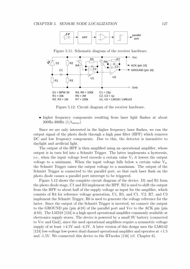
CHAPTER 5. SENSOR NODE LOCALIZATION 127
HPFparallel
port
Figure 5.11: Schematic diagram of the receiver hardware.
D1
R1
R2
R3
R4
U1 U2
Vcc
Gnd
C1 C2C3
R5R6
R7
D1 = BPW 34R1 = 33kR2, R3 = 1M
R4, R6 = 100kR5 = 2MR7 = 100k
C1 = 15pC2, C3 = 1p
ACK (pin 10)
GROUND (pin 18)
U1, U2 = LM318 / LM6142
-
+
+
-
Figure 5.12: Circuit diagram of the receiver hardware.
• higher frequency components resulting from laser light flashes at about200Hz-300Hz (1/tmirror)
Since we are only interested in the higher frequency laser flashes, we run theoutput signal of the photo diode through a high pass filter (HPF) which removesDC and low frequency components. Due to this, the detector is insensitive todaylight and artificial light.
The output of the HPF is then amplified using an operational amplifier, whoseoutput is in turn fed into a Schmitt Trigger. The latter implements a hysteresis,i.e., when the input voltage level exceeds a certain value V1 it lowers the outputvoltage to a minimum. When the input voltage falls below a certain value V2,the Schmitt Trigger raises the output voltage to a maximum. The output of theSchmitt Trigger is connected to the parallel port, so that each laser flash on thephoto diode causes a parallel port interrupt to be triggered.
Figure 5.12 shows the complete circuit diagram of the device. D1 and R1 formthe photo diode stage, C1 and R3 implement the HPF. R2 is used to shift the outputfrom the HPF to about half of the supply voltage as input for the amplifier, whichconsists of R4 for reference voltage generation, U1, R5, and C1. U2, R7, and C3implement the Schmitt Trigger, R6 is used to generate the voltage reference for thelatter. Since the output of the Schmitt Trigger is inverted, we connect the outputto the GROUND pin (pin #18) of the parallel port and Vcc to the ACK pin (pin#10). The LM318 [124] is a high speed operational amplifier commonly available atelectronics supply stores. The device is powered by a small 9V battery (connectedto Vcc and Gnd), since the used operational amplifiers require a symmetric voltagesupply of at least +4.5V and -4.5V. A later version of this design uses the LM6142[124] low-voltage low-power dual channel operational amplifier and operates at +1.5and -1.5V. We connected this device to the BTnodes [116] (cf. Chapter 6).

CHAPTER 5. SENSOR NODE LOCALIZATION 128
volta
ge
time
turn - t beamOR tt beam
tmirror
Figure 5.13: Input voltage at the parallel port as beams pass by the photo detector.
The receiver software consists of two main components, a Linux device driverwhich handles the parallel port interrupt, and an application level program whichperforms the actual location computation and lighthouse calibration. The devicedriver mainly consists of the parallel port interrupt handler, which is implementedusing the parapin [125] parallel port programming library. Moreover, it implementsa Linux special device /proc/location, which provides a simple interface to user-level applications. By writing simple ASCII commands to this device, a user-levelprogram can instruct the device driver to do some action.
The supported commands are:
• init: Create a new lighthouse. The driver initializes data structures fora new lighthouse and autodetects the rotation speed tmirror of a previouslyundetected lighthouse.
• reset N: Reset lighthouse N to the initial state.
• clear: Delete all active lighthouses.
• rounds N M: Instruct the driver to take into account M lighthouse turns andoutput the mean of the M measurements for lighthouse N.
By reading the /proc/location device, a user-level program can obtain the currentstatus and measured angle α according to Equation 5.10 of all detected lighthouses.A sample output line looks as follows:
lh0: seq 1, angle 1857, pulse 4232us, rounds 1
indicating that lighthouse 0 has tmirror = 4232µs, α = 0.01857 (the value is scaledby 100000), has done one measurement (sequence number 1), and is taking intoaccount 1 lighthouse turn for each measurement.
In order to measure α, the driver has to evaluate the interrupts it sees. Tounderstand how this is done, consider Figure 5.13, which shows the input voltage

CHAPTER 5. SENSOR NODE LOCALIZATION 129
at the parallel port over time. As the first rotating laser beam passes by the photodetector, the parallel port sees a sequence of sharp pulses resulting from the fastrotating mirror. The pulses stop when the lighthouse platform has turned enoughso that the photo detector isn’t hit any longer by the rotating beam. After sometime, the second rotating beam passes by the photo detector and again generatesa sequence of fast pulses.
Recall that each pulse generates an interrupt, which results in the device driverinterrupt handler being invoked. The handler then uses the system clock (whichhas µs resolution under Linux) to determine the point in time when the interruptoccurred.
The time interval between two successive fast pulses equals the time tmirror
for one rotation of the mirror. Since each lighthouse has a different tmirror, thisvalue can be used to distinguish different lighthouses. Please note that the pulsesequences can contain “holes” where the laser beam missed the photo detector dueto vibrations. The driver removes all peaks separated by holes from the beginningand the end of the sequence of pulses. The time midpoint of the resulting shortersequence of pulses without holes is assumed as the detection time of the beam(indicated by the braces in Figure 5.13).
Recall from Section 5.4.2, that we implemented a “virtual” wide beam by tworotating laser beams that form the outline of this wide beam. Therefore, the timepassed between the midpoints of two successive packs is either tbeam or tturn− tbeam.If the actual value is small (e.g., < 1sec) then it is assumed to be tturn. If thelighthouse has just been initialized the driver also measures tturn− tbeam in order toobtain tturn. Since the latter does not change, this has to be done only once. Lateron, the driver can output a new α with each round of the lighthouse.
In order to distinguish successive pulses from “holes”, and holes from “beamswitches”, the driver knows tight lower and upper bounds for the possible valuesof tmirror and tturn. In Section 5.4.3 we mentioned the possibility that beams fromdifferent lighthouses may hit the photo receiver at the same time. If this happensthe resulting time between successive pulses will fall below the lower bound fortmirror, such that the driver can detect this situation instead of producing faultyresults.
Using the /proc/location interface of the device driver, the user-level programimplements lighthouse calibration and location computation. The program is moreor less a straightforward implementation of the concepts developed in Section 5.4.2.
A simplified version of this software also runs on the ATMEL microcontrollerof the BTnodes. This setup more closely resembles the limited capabilities of aSmart Dust node and allows us to study the potential effects of a Smart Dust nodeon the location system (cf. Chapter 6).
5.4.4 Evaluation
In this section we examine the compliance of the Lighthouse Location System withthe region in the design space indicated in Section 5.3 and examine additional

CHAPTER 5. SENSOR NODE LOCALIZATION 130
���������������������������������������������������������������������������������������������������������
���������������������������������������������������������������������������������������������������������
���������������������������������������������������������������
���������������������������������������������������������������
���������������������������������������������������������������������������������������������������������
������������������������������������������������������������������������������������������������������������������������������
���������������������
x
x
Figure 5.14: Ensuring mutually perpendicular lighthouses.
aspects of the system, namely factors that influence the precision of the locationestimates, limits on the maximum distance of nodes from the base station, theeffects of node mobility, and the cost of adding localization support to dust nodes.We begin with examining the calibration of the lighthouse beacon as a prerequisitefor quantifying the precision of our approach.
Calibration
Calibration of the base station involves the following three steps:
• Ensuring that the lighthouses are mutually perpendicular.
• Measuring the offsets of the lighthouse centers x0 and z0.
• Determining Cb, Cβ, Cγ, Cδ for each of the two lighthouses.
In order to ensure that the two lighthouses are mutually perpendicular, we placedthe base station at the corner of a rectangular room as depicted in Figure 5.14,such that the rotation axes of the two lighthouses are at distance x from the twoperpendicular walls. We disabled the motors that drive the rotating mirrors andone of the two lasers of each lighthouse. Then we adjusted the mirror so that theremaining laser beam points at the opposite wall. Due to the rotating lighthouseplatforms, the laser spots draw two circles on the walls. The centers of these twocircles mark the position where the lighthouse rotation axes hit the wall as depictedin Figure 5.14. Now we adjust the lighthouses on the common chassis such that thecenters of these circles also have a distance x from the walls. In our measurementsetup, we placed the base station at x = 20cm in a room with a size of about 5mby 5m.
As mentioned in Section 5.4.2, the lighthouse center offsets x0 and z0 from theorigin of the coordinate system defined by the lighthouse rotation axes are not

CHAPTER 5. SENSOR NODE LOCALIZATION 131
[m]
0 1 2 3 4 5
[m]
0
1
2
3
4
5
c c c c cc c c c cc c c c cc c c cc c c
Figure 5.15: Location estimation benchmark. The ground truth locations are atthe centers of the circles. The mean of the measured locations are at the centersof the boxes. The edge length of each box is twice the standard deviation in eachaxis.
critical for the accuracy of the system. Therefore, we measured them directly atthe base station device.
In order to determine the C∗ values, we placed the observer at the four locations(x, z) ∈ {(50, 50), (480, 80), (80, 480), (340, 340)} (all values in centimeters) on thefloor in the base station coordinate system. The respective lighthouse distance andheight values are obtained from the (x, z) values as follows:
(dx, hx) := (z, x− x0)(dz, hz) := (x, z − z0)
(5.25)
At each of the locations, we performed ten measurements of α for each lighthouseand computed the mean value. For each of the two lighthouses we then solvedEquation System 5.21 in order to obtain the C∗ values.
Precision
For the precision benchmark, we placed the observer at 22 locations on the grid(80cm + i ∗ 100cm, 80cm + j ∗ 100cm) in the base station coordinate system on thefloor of the room. At each of the locations, we measured the location ten times byiteratively solving Equation System 5.19 as described in Section 5.4.2.
Figure 5.15 shows the base station coordinate system and the results of thesemeasurements. Ground truth locations (x, z) are indicated by circles. The mean ofthe computed location (x, z) is at the center of the small boxes. The edge length
CHAPTER 5. SENSOR NODE LOCALIZATION 132
of each box is twice the standard deviation sx (sz) of the measurements in therespective axis.
Please note that we determined ground truth locations using a cheap 5m tapemeasure, resulting in a maximum error of about ±1cm in each axis. Also note thatwe did not perform outlier rejection or any other statistical “tricks” to improve themean values or standard deviations.
The mean relative offset of the mean locations from ground truth locations(i.e., |x − x|/x) is 1.1% in the x axis, and 2.8% in the z axis. The overall meanrelative offset of the mean locations from ground truth locations (i.e., |(x, z) −(x, z)|/|(x, z)| is 2.2%. The mean relative standard deviation (i.e., sx/x) is 0.71%in the x axis and 0.74% in the z axis. The overall mean relative standard deviation(i.e., s|(x,z)|/|(x, z)|) is 0.68%.
Sources of Imprecision
In this section we examine which factors influence the accuracy of the system. Forthis, we have to examine errors that can occur during the measurement of tbeam
and tturn. From a measurement point of view, the two are identical, since they areboth an amount of time elapsed between two beam sightings. Therefore we willuse t as a genus for the two and ∆t as the absolute error of t. The following listcontains possible causes for measurement errors:
• Vibrations: Due to their fast rotation, the mirrors and thus the reflectedbeams suffer from small vibrations, resulting in a small angle ε of beamspread, which is about 0.05◦ in our prototype. Assuming sin ε = ε (since ε ≈0), the resulting error is ∆t ≤ tturn
ε√
d2+h2
2πdfor an observer located at distance
d from the lighthouse rotation axis and at height h over the lighthouse center.
• Lower bound on time tmirror for one mirror rotation: Since we can measureelapsed time only when the rotating laser beam hits the photo detector, theaccuracy of tbeam and tturn is limited by the speed of the rotating mirrors (i.e.,tmirror). The resulting error is ∆t ≤ tmirror.
• Flutter of platform rotation: The relative error in lighthouse rotation speedρlh causes an error in t. ρlh is mainly caused by the flutter of the motor drivingthe lighthouse platform. The motor used in our prototype has a flutter of0.1%. The resulting error is ∆t ≤ tρlh.
• Variable delays: There is a variable time offset between the laser beam hittingthe photo detector and the interrupt handler reading the clock. On the pathfrom the photo detector to the interrupt handler are many sources of variabledelay, such as hardware and interrupt latency. The actual value of this errorpretty much depends on what is currently happening on the computer, butis typically small compared to the other sources of errors.

CHAPTER 5. SENSOR NODE LOCALIZATION 133
l
d
t 1t 2
Figure 5.16: The photo detector must be hit by the laser beam at least twice.
• Clock resolution: The minimum time unit tmin that can be measured by theclock limits the time resolution for measurement of t. The Linux laptopwe used has tclockres = 1µs. On the ATMEL we used a 16-bit counter toimplement a clock with tclockres = 50µs. The resulting error is ∆t ≤ tclockres.
• Clock drift: The maximum relative error ρclock in the clock rate also causesan error in t. A typical value is ρclock = 10−5 both on Linux and the ATMEL.The resulting error is ∆t ≤ tρclock.
In our prototype system, the clearly dominating errors are caused by vibrations,limited tmirror, and flutter of platform rotation. The use of deflectable MEMSmirrors can both drastically reduce vibrations and tmirror. The flutter of platformrotation can be reduced to about 0.01% by using electronically stabilized motorsas used, for example, in turntable drives. By this, we expect a possible reductionof ∆t by a factor of about 10.
Note, however, that the errors resulting from these three main sources canbe modeled by a Gaussian noise source. This means that averaging over a largenumber of measurements helps to reduce the error.
Range
In this section we examine the maximum range, at which observers can still deter-mine their location. This maximum range mainly depends on two issues. The firstof these issues is that the photo receiver has to be hit twice by each of the rotatingbeams in order for the receiver to identify the lighthouse as explained in Section5.4.3. Figure 5.16 depicts this situation. It shows a top view of a lighthouse withonly one of the two rotating beams at two points in time t1 and t2. At t1, thebeam hits the photo detector at distance d from the lighthouse rotation axis thefirst time. Then, the mirror does one rotation and hits the photo detector a secondtime at t2. During t2 − t1, the lighthouse platform has rotated a bit to the left. ldenotes the diameter of the photo detector. Assuming a constant diameter w ofthe laser beam, the distance d at which the photo detector is hit at least twice isgiven by the following inequality:

CHAPTER 5. SENSOR NODE LOCALIZATION 134
d <l + w
2 sin(πtmirror/tturn)(5.26)
With the values of our prototype system l = 5mm, w = 3mm, tmirror = 4ms,tturn = 60sec we can achieve a theoretical maximum range of about 14m. Thisvalue can be improved by increasing tturn, by decreasing tmirror, or by defocusingthe lasers a bit, such that there is a small angle of beam spread. However, there arecertain limits for each of these possibilities. The angle of beam spread is limitedby the sensitivity of the photo detector and the output power of the laser. tmirror
is limited by the possible maximum speed of the mirrors. With MEMS deflectablemirrors such as the one presented in [25], we can achieve tmirror = 1/35kHz = 30µs.tturn is limited by the frequency of location updates needed by the nodes and thusby the degree of node mobility (see Section 5.4.4).
The second issue that limits the maximum range of the system is the speedof the photo detector. Using commercial-off-the-shelf technology, the beam hasto stay on the photo detector for about tphoto = 10ns in order to be detected.Depending on the minimum retention period tphoto of the laser beam on the photodetector, the maximum distance d is limited according to the following inequality:
d <l + w
2 sin(πtphoto/tmirror)(5.27)
With the current values of our prototype tphoto = 200ns, tmirror = 5ms, l = 4mm,w = 3mm we can achieve a theoretical maximum range of about 27m, giving us anoverall range limit of 14m. Again, this value can be improved by reducing tmirror
and by defocusing the laser with the same limits as above.The actually measured maximum range, at which the receiver prototype could
still detect the base station is about 11 meters. However, the range can be in-creased by adjusting certain system parameters. A more elaborate system builtusing fast deflectable MEMS mirrors with values l = 1mm, w = 20mm (due tobeam spread), tmirror = 1ms, tturn = 60sec, and tphoto = 10ns, for example, couldachieve a theoretical maximum range of about 210m (the minimum obtained fromInequalities 5.26 and 5.27). Based on our experience, we would expect a practi-cal maximum range of about 120-140m of a system with these parameters, whichapproximately equals the maximum communication range of 150m during the dayfor the Berkeley experiments [49].
Resources
In this section we want to examine how the presented location system fits thestringent resource restrictions of future Smart Dust Systems. These restrictionsespecially apply to the receiver side, i.e., the Smart Dust nodes.
The Berkeley Smart Dust prototype has already demonstrated that a photodetector similar to the one we are using for our location system is feasible. Whatremains to be shown is how the receiver software (i.e., the device driver and theuser-level program) fit onto a Smart Dust node.

CHAPTER 5. SENSOR NODE LOCALIZATION 135
Both the processing overhead and the memory footprint of the device driverare very low, which is very important for Smart Dust. The first is true becausethe driver is interrupt driven, i.e., it does not do any sensor sampling or polling.Moreover, the interrupt can be used to wake up the processor from a power-savingmode. Thus, the system has to be woken up only during the short periods when abeam is hitting the photo detector. The memory footprint is very low because thedriver does not have to store arrays of peak detections. Instead, for each sequenceof peaks it only keeps “first peak” and “last peak” time stamps which are updatedwhen a new interrupt occurs. The whole data structure for one lighthouse onlyrequires about 25 bytes.
Similarly, the location-computation part of the user-level program has a verylow memory footprint. It just retrieves the α values from the device driver and ex-ecutes the approximation program described in Section 5.4.2. Given the relativelyinfrequent location updates, speed is not a problem. On computationally very lim-ited platforms like future Smart Dust nodes, it might be necessary to revert tofixed point arithmetic and a hardware implementation of the location computa-tion code in case the provided processing capabilities are too limited. Besides thebasic arithmetic operations (+,−, ∗, /) we need support for sin α and
√x in order
to solve Equation System 5.19. Note that sin α is easy to approximate since thevalues of α obtained from Equation 5.10 are small due to tbeam � tturn. The secondorder approximation sin α ≈ α− α3/6 has a maximum error of 0.1% for |α| ≤ 33◦.There are also fast approximations for y =
√x. One possible approach is to first
approximate 1/√
x by iterating y := y(3− xy2)/2 with an appropriate initial valuefor y. Multiplying the result by x gives an approximation for
√x.
The requirements on the clock are also quite relaxed. Note that we don’t needa real-time clock since we are only interested in the quotient tturn/tbeam. A simplecounter which ticks at a constant rate would also be sufficient. The resolution ofthe clock (or counter) just has to be high enough to reliably distinguish the tmirror
values of different lighthouses. Since the tmirror values of our prototype system are4ms and 5ms, respectively, a clock resolution of 0.5ms would be sufficient.
Please note that dust nodes don’t have to be calibrated due to the followingtwo reasons. Firstly, the two beam sightings used to measure tbeam and tturn areidentical from a measurement point of view. Any constant hardware and softwaredelays will subtract out. Secondly, only the quotient tturn/tbeam is used for nodelocalization, which is independent of the actual clock frequency.
Node Mobility
If nodes change their location over time, they have to update their location esti-mates frequently in order to avoid inaccuracies resulting from using outdated loca-tion estimates. Moreover, node movement during the measurement of parametersneeded for location computation can cause inaccuracies in the estimated location.
The time tupdate between successive location updates usually equals the time tturn
required for one rotation of the lighthouse. Thus, the update frequency 1/tupdate
can be increased by decreasing tturn. However, there is an easy way to double the

CHAPTER 5. SENSOR NODE LOCALIZATION 136
update frequency when using rotating mirrors for beam generation, because thebeams are reflected to both sides of the lighthouse as depicted by the dashed laserbeams in Figure 5.8. Thus, we actually have two “virtual” wide beams we can usefor location estimation, effectively doubling the update frequency.
If a node moves during measurement of tbeam (i.e., after detection of the firstbeam and before detection of the second beam), the obtained value of tbeam will beincorrect. Additional errors are caused by the node moving between measurementsof tbeam of the three lighthouses.
There are two ways to detect and reject faulty location estimates resulting fromnode movement during measurement. The first compares two or more consecutiveposition estimates and rejects them if they differ by more than a small threshold.The second approach uses accelerometers to detect movement during measurement.Accelerometers can also be used to estimate node movement (velocity, direction)during measurements of tbeam. The obtained values can be used to correct tbeam,such that correct location estimates can also be obtained during node movement.In fact, the Smart Dust prototypes developed at Berkeley already contain suchsensors.
Line-Of-Sight Requirement
As mentioned in Section 2.5.3, communication between a node and the base stationrequires an uninterrupted line of sight (LOS) even for “plain” Smart Dust (i.e.,without using the Lighthouse Location System). Hence, the presented locationsystem does not introduce additional restrictions with respect to LOS.
Temporary LOS obstructions can cause wrong position estimates if a dust nodemisses one of the laser beams. However, the probability of such errors can bereduced by comparing two or more consecutive positions estimates and rejectingthem if they differ by more than a small threshold. Reflected laser beams aretypically not detected by the receiver hardware, since diffuse reflection reduces thelaser light intensity drastically.
Note that other localization systems based on ultrasound and radio waves pro-vide location estimates even in the case of an obstructed line of sight. However, theresulting location estimates are typically wrong due to relying on signals reflectedaround the obstruction. Often it is difficult to detect such situations [42], whichmay result in using wrong location estimates unnoticed.
Robustness
We assume that base stations are immobile and mounted in a safe place (withrespect to harmful environmental influences) due to their potential long range (seeSection 5.4.4). On the other hand, dust nodes are subject to mobility and otherkinds of environmental influences (e.g., LOS obstructions), which can cause faultylocation estimates.
However, above we mentioned extensions to the basic system in order to detectand reject such faulty location estimates with high probability. This leaves us in a

CHAPTER 5. SENSOR NODE LOCALIZATION 137
situation, where dust nodes either obtain good position estimates or none at all.
5.5 Summary
This chapter is devoted to node localization in wireless sensor networks. We firstdiscussed important models with respect to mobility and signal propagation. Fol-lowing the framework developed in Chapter 3, we then presented important con-cepts used by localization algorithms. Referring to these concepts, we then pre-sented and discussed important existing approaches to localization – both in tra-ditional distributed systems and for sensor networks. We then identified a regionin the design space that cannot be appropriately supported by these existing algo-rithms. In particular, we showed that tiny sensor nodes known as Smart Dust arenot sufficiently supported. We presented and evaluated the Lighthouse LocationSystem to support this region in the design space. A key feature of this approachis that sensor nodes can autonomously infer their location by observing laser lightflashes emitted by a special lighthouse device. We showed that this approach isefficient since sensor nodes do not actively emit any signals. Based on a prototypi-cal implementation, we evaluated the precision of this approach and found that anaccuracy in the order of centimeters can be achieved. We also discussed potentialimprovements to further increase the precision.
Chapter 6
Application Experience
In this chapter we present a prototypical application in order to demonstrate thepractical feasibility and usability of the approaches for time synchronization andnode localization we developed in Chapters 4 and 5.
The application supports tracking the location of a mobile object – a remote-controlled toy car in our example. For this, a number of sensor nodes are deployedin the area of interest, each equipped with a sensor to detect the proximity of themobile object. In order to estimate the current location of the tracked object, thelocations of the sensor nodes in space and time must be known with respect to acommon coordinate system.
In Section 6.1 we describe the general setup of the application, details are givenin Sections 6.2-6.6. The tracking system is evaluated and discussed in Sections 6.7and 6.8.
6.1 Object Tracking with Smart Dust
The purpose of our prototypical application is to track the location of real-worldphenomena with a network of Smart Dust nodes. We use a remote-controlled toycar (Figure 6.1) as the tracked object. The current tracking system assumes thatthere is only one car. Sensor nodes are randomly deployed in the area of interestand can change their location after deployment. When they detect the presenceof the car (cf. Section 6.2), they send notifications to a base station. The basestation fuses these notifications (cf. Section 6.3) in order to estimate the currentlocation of the car. A graphical user interface displays the track and allows tocontrol various aspects of the system. The data fusion process requires that allnodes share a common reference system both in time and space, which necessitatesmechanisms for node localization (cf. Section 6.4) and time synchronization (cf.Section 6.5).
Since Smart Dust hardware has not been available to us, we used BTnodes[116] to mimic the behavior of Smart Dust (cf. Section 2.5.3). Figure 6.2 showsa complete sensor node as used in our application. The base station consists of aLinux laptop computer equipped with a Bluetooth radio. In analogy to the single-
138

CHAPTER 6. APPLICATION EXPERIENCE 139
IR emitter
Figure 6.1: A remote-controlled toy car with an IR emitter is used as the trackedobject.
IR detectorlocationsensor
BTnode
Figure 6.2: A BTnode with an IR detector and lighthouse receiver is used as aSmart Dust surrogate.
hop network topology of Smart Dust, BTnodes do not directly communicate witheach other, but only with the base station. Before communication can take place,the base station has to set up a so-called Bluetooth Piconet containing no morethan 7 BTnodes. To support more than 7 nodes, the base station has to periodicallyswitch the Piconet in a round robin fashion, such that eventually every BTnodegets a chance to talk to the base station. Note the analogy to Smart Dust, wherethe base station has to point the (typically slightly defocused) laser beam at agroup of nodes in order to enable communication with them.
6.2 Object Detection
Tracking objects with networks of sensors has been an active research topic formany years, [23, 55, 103] give a good overview of many tracking algorithms. Mostof the approaches are optimized for sparse networks, where a high tracking accuracy

CHAPTER 6. APPLICATION EXPERIENCE 140
should be achieved despite a relatively low node density. To achieve this, manyapproaches make a number of assumptions about the tracked object. Methodswhich estimate object distance based on signal strength estimates, for example,require knowledge of the intensity of the signal emitted by the object in order toachieve good accuracy. Approaches based on measuring at different sensor nodesthe difference of time of arrival of a signal emitted by the object are typicallylimited to sound or other signal modalities with low propagation speed. Signalmodalities with high propagation speeds such as radio waves (e.g., light) wouldrequire distributed clock synchronization with an accuracy of few nanoseconds,which is typically not feasible. Other approaches require known lower and upperbounds of the velocity or the acceleration of the tracked object.
While these assumptions help to achieve good tracking accuracy, they also limitthe applicability of the tracking system. In order to make our system applicable toa wide variety of objects, we tried to avoid making assumptions about the target asmuch as possible. In order to achieve a satisfactory tracking accuracy nevertheless,we exploit the anticipated high density of Smart Dust deployments – which isexpected because of the intended small size and low cost of Smart Dust devices.
Our approach assumes that the presence of the target object can be detectedwith an omnidirectional sensor featuring an arbitrary but fixed sensing range r,that is, the sensor can “see” the target only if the distance to the target is lowerthan r. The data fusion algorithm presented in the following section needs to knowan upper bound R of this sensing range. In many applications, the target cannotbe instrumented for tracking purposes (e.g., a cloud of toxic gas, an oil slick, fire).The remote-controlled car we used as a sample target in our tracking system emitsa characteristic acoustic signature which could be used for detection. However,this signature depends on the velocity of the car. To avoid the intricacies withdetecting this variable signature, we chose in our experiment a different solutionbased on infrared (IR) light, leaving detection based on the car’s acoustic signatureas future work.
In the current version of the prototype, we equipped the car with an omni-directional IR light emitter consisting of eight IR LEDs mounted on top of thecar (Figure 6.1). Accordingly, the sensor nodes are equipped with an omnidirec-tional IR light detector consisting of three IR photo diodes (Figure 6.2). Theused IR photo diodes include a filter to cancel out visible light. The output ofthe IR detector is connected to an analog-to-digital converter (ADC) of the BTn-ode’s microcontroller. If the output value of the ADC exceeds a certain threshold,the presence of the car is assumed. Using a low-pass filter, the threshold value isadopted to slowly changing daylight, which also contains IR components. With thissetup, the BTnodes can detect the car at a distance of up to approximately halfa meter. When a node first detects the car, it sends a “detection notification” tothe base station, containing its node ID as well as its time and location at the timeof detection. When the node no longer sees the car, it sends a “loss notification”to the base station, which contains its node ID and its current time. If the nodechanges its location during the presence of the car, a loss notification is emitted,

CHAPTER 6. APPLICATION EXPERIENCE 141
11
22
Figure 6.3: Estimating object location by centroids.
followed by a detection notification with the new node location.
6.3 Data Fusion
Following the argumentation at the begin of the Section 6.2, we try to avoid makingassumptions about the target as much as possible. Therefore, the base stationhas to derive the current location of the tracked object solely based on detectionnotifications and loss notifications received from the sensor nodes.
We use an approach that estimates the car’s location at time t by the centroid ofthe locations of the sensor nodes that “see” the car at time t. The centroid of a set ofN locations {li = (xi, yi, zi)} is defined as l := 1
N
∑li =
(1N
∑xi,
1N
∑yi,
1N
∑zi
).
Consider Figure 6.3 for an example. Depicted are three sensor nodes (black squares)with their respective sensing ranges, and two car locations (black circles). Thehollow circles indicate the respective estimated locations (i.e., centroids).
Figure 6.4 illustrates an algorithm to calculate the car location estimates giventhe detection and loss notifications received from the sensor nodes as described inSection 6.2. The figure shows sensor nodes 1 and 2, their respective sensing ranges,and the trajectory of the car (dotted arrow). When the car enters the sensing rangeof node i, a detection notification di is emitted, containing time di.t and locationdi.l of node i at the time of detection. Accordingly, node i emits a loss notificationli when the car leaves the sensing range. In a first step, all notifications are sortedby increasing time stamps di.t (li.t) as depicted on the time axis in the lower halfof Figure 6.4. In a second step, we iterate over these sorted notifications from leftto right, recording the active nodes (those that currently see the car) in a set S.If we come across a loss notification li, we remove i from S. If we come acrossa detection message di, we add i to S. Additionally, we remove all nodes j fromS, whose sensing ranges do not overlap with the detection range of node i, thatis, for which |di.l − dj.l| > 2R holds. This is necessary to compensate for missedloss notifications, which would otherwise permanently affect the accuracy of thetracking system by not removing the respective entries from S. A missing enternotification will lead to a temporarily decreased tracking accuracy, but will not

CHAPTER 6. APPLICATION EXPERIENCE 142
1 2
d
d 2
l1
l2
1
timed .t1 d .t2 l .t1 2
estimatedlocation
2
2d .l1 d .l2
d .l + d .l1
l .t
Figure 6.4: Data fusion algorithm.
otherwise permanently affect the system.The location of the car during the time interval starting at the currently consid-
ered notification and ending at the next notification is estimated by the centroid Sof the locations of the nodes in S (i.e., d1.l during [d1.t, d2.t), (d1.l + d2.l)/2 during[d2.t, l2.t), and d2.l during [l1.t, l2.t)).
The localization accuracy of a similar centroid-based algorithm was examinedin [17] in a different context under the assumption that nodes are located on aregular grid. We can interpret their results for our setting as follows. The local-ization accuracy depends on the sensing range r of the nodes (about 50 cm in ourcase) and the distance d between adjacent nodes. For r/d = 2 (i.e., d ≈ 25 cmin our case) the average and maximum localization errors are 0.2d (i.e., 5 cm) and0.5d (i.e., 12.5 cm), respectively. In general, larger r/d values yield better accu-racy. Therefore, the accuracy can be improved by increasing the node deploymentdensity, since that reduces d while keeping r constant.
6.4 Node Localization
In order to derive the location of the tracked car from proximity detections asdescribed in Section 6.2, the locations of the sensor nodes have to be estimated.We used the Lighthouse Location System for this purpose. The receiver hardwaredescribed in Section 5.4.3 was connected to a digital input pin of the ATMELmicrocontroller, such that every light flash triggers an interrupt. A simplifiedversion of the receiver software (omitting support for calibration) has been portedto the ATMEL.

CHAPTER 6. APPLICATION EXPERIENCE 143
6.5 Time Synchronization
The car location estimation described in Section 6.3 assumes that the timestampscontained in notification messages refer to a common physical time scale. We usedTime-Stamp Synchronization for this purpose. We implemented a slight variationin order to relief the base station from keeping state information for every node(cf. Section 4.4.4). This can be achieved by sending this state information to thenode as part of the acknowledgment message. A node must then include this stateinformation in the next event notification to make it again available to the basestation. This way, every node is responsible for storing its own state.
6.6 Message Ordering
The data fusion algorithm described in Section 6.3 requires sorting notificationsby their time stamps. The time transformation approach described in Section6.5 enables us to compare and sort time stamps originating from different nodes.However, we still have to ensure that a notification message is not processed by thedata fusion algorithm until all earlier notifications have arrived at the base station.This is of particular importance for Smart Dust, since messages are subject to longand variable delays as described in Section 2.5.3.
One particularly attractive approach to message ordering is based on the as-sumption that there is a known maximum network latency D. Delaying the evalu-ation of inbound messages for D will ensure that out-of-order messages will arriveduring this artificial delay and can be ordered correctly using their time stamps.That is, message ordering can be achieved without any additional message ex-changes. The literature discusses a number of variants of this basic approach[59, 70, 94].
However, there is one major drawback of this approach: the assumption ofa bounded and known maximum network latency. Since communication requiresthat the base station points its laser at a node, Smart Dust suffers from long andvariable network delays. Using a value for D which is lower than the actual networklatency results in messages being delivered out of order. Using a large value for Dresults in long artificial delays, which unnecessarily decreases the performance ofthe tracking system.
We therefore introduce a so-called adaptive delaying technique that measuresthe actual network delay and adapts D accordingly. Doing so, it is possible thatthe estimated D is too small and messages would be delivered out of order. Our al-gorithm detects such late messages and deletes them (i.e., does not deliver them tothe application at all). Recall that the data fusion algorithm presented in Section6.3 was specifically designed to tolerate missing detection and loss notifications.Hence, deleting a message only results in a less accurate track, since the affectedSmart Dust node simply does not contribute to the estimation of the target loca-tion. We argue that this slight decrease of accuracy is acceptable since deletinga message is a rare event, which only occurs at startup or when the maximum

CHAPTER 6. APPLICATION EXPERIENCE 144
network latency increases during operation (i.e., when the value of D is lower thanthe actual maximum network latency). The expected high density of Smart Dustdeployments can also compensate this decrease of accuracy. Additionally, our al-gorithm includes a parameter which can be tuned to trade off tracking latency fortracking accuracy.
Specifically, the adaptive delaying algorithm executed in the base station main-tains a variable D holding the current estimate of the maximum delay, a variabletlatest holding the time stamp of the latest message delivered to the application,and a queue which stores messages ordered by increasing time stamps. Initially, Dis set to some estimate of the maximum network latency, tlatest is set to the currenttime tnow in the base station, and the queue is empty.
Upon arrival of a new notification n with time stamp (interval) n.t, the actualmessage delay d := tnow − n.tl is calculated1. D is then set to the maximum of Dand c · d. The constant factor c influences the chance of having to delete an out-of-order message and can thus be tuned to trade off tracking latency for trackingaccuracy. We use c = 1.2 in our prototype. Now we check if tlatest < n.tl holds, inwhich case n can still be delivered in order. If so, n is inserted into the queue atthe right position according to n.t. Otherwise, n is deleted.
The first element n0 of the queue (i.e., the one with the smallest time stamp)is removed from the queue as soon as the base station’s clock (tnow) shows a valuegreater than n0.t
r + D. Now tlatest is set to n0.tr and n0 is delivered to the data
fusion algorithm.
6.7 Evaluation
In order to assess the precision of the proposed tracking system, we performed a setof measurements. Figure 6.5 shows the setup of our measurements. The lighthousebeacon (“LH” in the picture) was placed in the upper left corner and defines theorigin (0,0) of a 2D coordinate system. Six sensor nodes (numbered rectangles inthe figure) were placed in an area of about one square meter. The car moved thenthrough the sensor field from right to left on a straight line. Location estimates wereobtained at 12 positions of the car (indicated by the black squares in the picture).We performed the whole experiment 10 times and calculated averages. The sensornodes as well as the car locations are annotated with coordinates (x± ex, y ± ey),where (x, y) are the ground truth positions in centimeters obtained by a tapemeasure. ±ex and ±ey indicate the average errors of the output of the trackingsystem relative to the ground truth position on the x and y axis, respectively.The average error of the sensor node location estimates is ex = 4.16 cm and ey =1.83 cm. We attribute the larger ex value to mechanical problems with one of thelighthouses. The average error of the car location estimates is ex = 12.5 cm andey = 3.5 cm. The maximum error of the sensor node location estimates is ex = 5 cmand ey = 2 cm. The maximum error of the car location estimates is ex = 28 cm
1tr (tl) refers to the right (left) end of the time interval t.
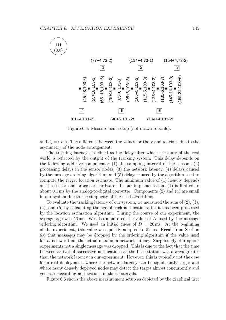
CHAPTER 6. APPLICATION EXPERIENCE 145
LH(0,0)
(77+4,73-2) (114+4,73-1) (154+4,73-2)
1 2 3
4 5 6
(61+4,131-2) (98+5,131-2) (134+4,131-2)
(45-
28,1
03-3
)
(55+
18,1
03-3
)
(65+
18,1
03+
6)
(75+
16,1
03-3
)
(85+
6,10
3-3)
(95+
6,10
3+3)
(105
+5,
103-
3)
(115
-5,1
03-3
)
(125
+4,
103-
3)
(135
-6,1
03-3
)
(145
-16,
103-
3)
(155
-22,
103+
6)
Figure 6.5: Measurement setup (not drawn to scale).
and ey = 6 cm. The difference between the values for the x and y axis is due to theasymmetry of the node arrangement.
The tracking latency is defined as the delay after which the state of the realworld is reflected by the output of the tracking system. This delay depends onthe following additive components: (1) the sampling interval of the sensors, (2)processing delays in the sensor nodes, (3) the network latency, (4) delays causedby the message ordering algorithm, and (5) delays caused by the algorithm used tocompute the target location estimate. The minimum value of (1) heavily dependson the sensor and processor hardware. In our implementation, (1) is limited toabout 0.1ms by the analog-to-digital converter. Components (2) and (4) are smallin our system due to the simplicity of the used algorithms.
To evaluate the tracking latency of our system, we measured the sum of (2), (3),(4), and (5) by calculating the age of each notification after it has been processedby the location estimation algorithm. During the course of our experiment, theaverage age was 56ms. We also monitored the value of D used by the messageordering algorithm. We used an initial guess of D = 20ms. At the beginningof the experiment, this value was quickly adapted to 52ms. Recall from Section6.6 that messages may be dropped by the ordering algorithm if the value usedfor D is lower than the actual maximum network latency. Surprisingly, during ourexperiments not a single message was dropped. This is due to the fact that the timebetween arrival of successive notifications at the base station was always greaterthan the network latency in our experiment. However, this is typically not the casefor a real deployment, where the network latency can be significantly larger andwhere many densely deployed nodes may detect the target almost concurrently andgenerate according notifications in short intervals.
Figure 6.6 shows the above measurement setup as depicted by the graphical user
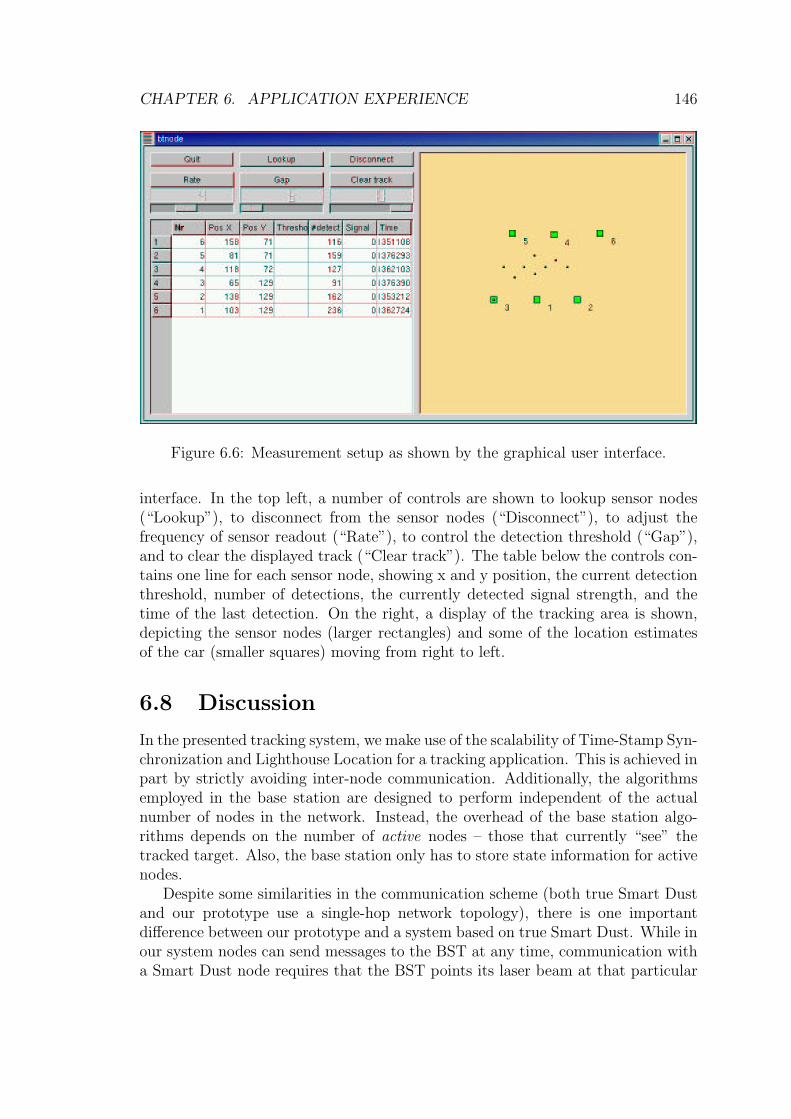
CHAPTER 6. APPLICATION EXPERIENCE 146
Figure 6.6: Measurement setup as shown by the graphical user interface.
interface. In the top left, a number of controls are shown to lookup sensor nodes(“Lookup”), to disconnect from the sensor nodes (“Disconnect”), to adjust thefrequency of sensor readout (“Rate”), to control the detection threshold (“Gap”),and to clear the displayed track (“Clear track”). The table below the controls con-tains one line for each sensor node, showing x and y position, the current detectionthreshold, number of detections, the currently detected signal strength, and thetime of the last detection. On the right, a display of the tracking area is shown,depicting the sensor nodes (larger rectangles) and some of the location estimatesof the car (smaller squares) moving from right to left.
6.8 Discussion
In the presented tracking system, we make use of the scalability of Time-Stamp Syn-chronization and Lighthouse Location for a tracking application. This is achieved inpart by strictly avoiding inter-node communication. Additionally, the algorithmsemployed in the base station are designed to perform independent of the actualnumber of nodes in the network. Instead, the overhead of the base station algo-rithms depends on the number of active nodes – those that currently “see” thetracked target. Also, the base station only has to store state information for activenodes.
Despite some similarities in the communication scheme (both true Smart Dustand our prototype use a single-hop network topology), there is one importantdifference between our prototype and a system based on true Smart Dust. While inour system nodes can send messages to the BST at any time, communication witha Smart Dust node requires that the BST points its laser beam at that particular

CHAPTER 6. APPLICATION EXPERIENCE 147
node. Even though a slightly defocused laser beam would enable the base stationto communicate with many Smart Dust nodes at a time, the laser has to sweep overthe deployment area to give each node a chance to talk to the base station. Wedeal with the resulting long and variable network delays by proposing a messageordering technique which adapts to the actual maximum network latency.
The data fusion algorithm used in our system might seem somewhat simplisticcompared to many approaches described in the literature. However, it achievesa reasonable accuracy while only making a minimum of assumptions about thetracked object. The loss of precision can be compensated by increasing the nodedensity – which is possible due to the expected small size and low cost of SmartDust nodes.
The tracking system has been designed to tolerate node failures, since these arelikely to happen. Messages lost due to node failures will only affect the accuracy ofthe estimated track. Again, this can be compensated by a higher node deploymentdensity.
6.9 Summary
This chapter shows the practical feasibility of our approaches for time synchroniza-tion and node localization using a concrete application. In particular, we showedhow Time-Stamp Synchronization and Lighthouse Localization can be used to im-plement a scalable tracking system based on Smart Dust. We also presented anapproach to implement message ordering for networks with long, variable delayssuch as Smart Dust. We also evaluated the precision of our prototype and foundthat it provides a precision in the order of tens of centimeters.

Chapter 7
Conclusions and Future Work
In this final chapter, we summarize the contributions of our work and discuss somelimitations of our approaches. We also sketch potential future work, both withrespect to the proposed algorithms and in the broader context of our work.
7.1 Contributions
We prosed a design space to replace the narrow definition of wireless sensor net-works that is currently assumed by most research papers. The selection of thedimensions of the design space was based on an extensive study of existing proto-typical applications. It was shown that these applications do indeed cover differentpoints in the design space. The identified dimensions of the design space deploy-ment, mobility, resources, heterogeneity, communication modality, infrastructure,network topology, coverage, connectivity, network size, and QoS requirements typ-ically have a significant impact on the design of specific solutions. We examinedthis impact on algorithms for time synchronization and node localization. In par-ticular, we identified important regions in the design space which are not coveredby existing solutions.
With respect to time synchronization, we showed that existing algorithms donot appropriately support intermittent and sporadic network connectivity. We pro-posed Time-Stamp Synchronization to overcome this lack. In contrast to existingschemes, this approach does not synchronize clocks. Rather, each unsynchronizedclock defines its own local time scale. Time-Stamp Synchronization transformstime stamps between these time scales as they are passed from node to node, alsoacross temporary network partitions. Moreover, synchronization can be performedon demand, where and when needed. Our approach uses intervals to representtime stamps. Therefore, reasoning about time stamps does not suffer from prob-lems due to synchronization errors. Also, our approach is efficient because it canoften piggyback time information on existing network traffic.
With respect to node localization, we showed that existing algorithms do notappropriately support tiny sensor nodes known as Smart Dust. We proposed theLighthouse Location System to overcome this lack. This approach is based on a
148

CHAPTER 7. CONCLUSIONS AND FUTURE WORK 149
new cylindrical lateration scheme, which allows Smart Dust nodes to autonomouslyestimate their locations with high precision using only a single external beacondevice that can be integrated with an existing base station. Since nodes do notrequire the support of other nodes for localization, this approach can scale to verydense networks, and localization can be performed on demand where and whenneeded.
We demonstrated the practical feasibility of the proposed solutions by imple-mentations that have also been used in a common prototypical application thatsupports tracking of mobile objects with a sensor network.
As one further contribution, we developed a common framework for discussingtime synchronization and node localization. In particular, we showed that manyexisting distributed algorithms for synchronization and localization share five com-mon structural elements: bootstrapping, obtaining constraints, combining con-straints, selecting constraints, and maintaining localization over time.
The major contributions of this thesis have also been published, most notablyin [34, 80, 82, 83, 84, 85, 86].
7.2 Limitations
The approaches to time synchronization and localization we proposed are tailoredto specific regions in the design space as discussed in Sections 4.3 and 5.3. Naturally,our approaches are less suited for other regions in the design space, resulting in anumber of limitations.
7.2.1 Time-Stamp Synchronization
Traditional time-synchronization schemes proactively synchronize clocks using aseparate protocol before the application may request synchronized time. Hence,these protocols can spend significant effort into achieving good precision. Forexample, they may perform multiple measurements to obtain many constraints. Incontrast, our scheme is designed to be performed on demand at the instant whenthe application requests synchronized time. To make such an approach feasible, theoverhead of synchronization must be kept to a minimum. For example, performingmultiple measurements is disadvantageous here, effectively limiting the precisionof time-stamp synchronization.
Time-Stamp Synchronization provides synchronization only for selected timeinstants. This is not sufficient for applications that require continuous synchro-nization over longer periods of time (e.g., performing periodic actions at a certainrate).
7.2.2 Lighthouse Location System
Localization with our approach requires a free line of sight between the lighthousebeacon and sensor nodes, which limits the applicability of this approach. Note,

CHAPTER 7. CONCLUSIONS AND FUTURE WORK 150
however, that the basic communication scheme of Smart Dust does also imposethis restriction. Hence, our localization system does not introduce an additionalconstraint here.
The geographical scale of networks that can be supported with our approachis limited by the range of the lighthouse beacon. The Lighthouse Location Systemuses range measurements to multiple lighthouses as a basic element. To obtaincorrect results, the sensor node must not move during the measurement. Hence,this approach cannot directly support nodes which are in constant movement unlessadditional sensors (e.g., acceleration) are used to compensate for movements duringmeasurement.
7.3 Future Work
There are a number of potential improvements with respect to our algorithms fortime synchronization and localization. However, we also discuss future work in thebroader context of our work, in particular with respect to the design space.
7.3.1 Time-Stamp Synchronization
For some applications it might be reasonable to strive for improved precision atthe cost of increased runtime overhead. Some directions which might be worthfurther investigation have been sketched in Section 4.4.9. Probability distributionsinstead of pure intervals would allow probabilistic reasoning about overlappingtime intervals. Such distributions could perhaps be constructed by taking intoaccount past message exchanges between a pair of nodes. A time-stamp historycould be included in each message to improve reasoning with time stamps thatpassed through a common node. However, this may result in significantly increasedmessages size.
7.3.2 Lighthouse Location System
It would be interesting to examine the use of deflectable MEMS mirrors or steerablelasers instead of rotating mirrors, since this could not only significantly improvethe precision of localization, but would also lead to a simplified and more robustlighthouse hardware. On the node side, an implementation on true Smart Dustwould gain significant insights into the feasibility of our approach on this hardwareplatform.
For networks with a large geographical extension, a single lighthouse beaconmay not be sufficient to cover the whole network. Here, multiple lighthouse bea-cons could be used. Future work would include an examination how a consistentcoordinate system could be established across a large network with multiple bea-cons. A natural approach would be to use clustering. Each lighthouse beacon woulddefine a cluster, such that all nodes in the cluster can receive the respective beacon.Each cluster uses the coordinate system defined by its lighthouse beacon. Nodes

CHAPTER 7. CONCLUSIONS AND FUTURE WORK 151
that are contained in multiple clusters could compute coordinate transformationsbetween adjacent clusters.
Another issue for future work is better support for mobility. As a first step,movement detectors could be used to detect faulty measurements, caused by a nodemoving during measurement. A second step would include movement compensa-tion, so that localization becomes also possible if a node is in constant travel. Suchan approach would require some form of dead reckoning (e.g., by means of acceler-ation sensors) to compensate the error in the sweep time measurement caused bynode movement.
7.3.3 Service Interfaces
Time synchronization and node localization can be considered as two basic servicesthat each provide one major function at its interface to the application: What isthe current time/location? However, as we have illustrated in this thesis, differentpoints in the design space may require vastly different approaches to provide thisbasic function in an adequate way. Also, concrete application requirements (e.g.,precision, scope, lifetime, mobility model) may necessitate different approaches fortime synchronization and node localization.
Despite these different requirements, modular programming could be greatlyenhanced if time synchronization and node localization services could be consideredbasic building blocks that provide a common interface across the design space. Thiswould, however, require the inclusion of methods into the interface that allow aspecification of the concrete requirements on the services, which might also changeduring the lifetime of the application. This raises the important question of howsuch an extended interface should look like. Broadly speaking, such an interfaceshould include methods to specify the exact point in the design space and additionalapplication requirements.
7.3.4 Service Selection and Adaptation
Different points in the design space and different application requirements typicallynecessitate different solutions for time synchronization and node localization. Insome cases, a single algorithm may provide parameters for adaptation to differentrequirements. In any case, an application developer is faced with the problem ofselecting an appropriate solution and/or appropriate parameters. If these require-ments change during the lifetime of an application, this choice may have to beupdated every now and then.
To relief application developers from these issues, frameworks and tools shouldprovide support for service selection and adaptation. Such system support is facil-itated by a common service interface as discussed in the previous section. By this,different service implementations become interchangeable. The interface elementsthat allow a user to specify application requirements and a point in the design spacecould then be used by the system to automatically select an appropriate service

CHAPTER 7. CONCLUSIONS AND FUTURE WORK 152
implementation.
7.3.5 Calibration
We can consider localization in both time and space as sensor calibration problems.Generally speaking, a sensor is a device that takes a certain physical quantity asinput and produces a variable electrical signal as output that is usually converted toa digital number using an analog-to-digital converter. Calibration then consists ofenforcing a certain mapping of the observed physical quantity to the sensor output.For example, if a sensor is exposed to a temperature of T ◦C, then the sensor shouldoutput T (in some reasonable digital encoding). Localization in space can then beconsidered as the task of calibrating a location sensor to a given coordinate system.Localization in time can likewise be considered as the task of calibrating a timesensor (e.g., a hardware clock) to a given coordinate system.
It would be worthwhile to examine the use of known techniques from timesynchronization and node localization in the more general context of calibration.It particular, it is quite likely that many of the observations in Chapter 3 couldbe generalized to calibration. For example, the classification in Section 3.2 can bedirectly transferred to calibration. It is also conceivable that distributed calibrationalgorithms could consist of structural elements similar to those we identified inSection 3.3.
7.4 Concluding Remarks
In this thesis we showed that applications of wireless sensor networks cannot becharacterized by a single, narrow definition, and we proposed a multi-dimensionaldesign space of Wireless Sensor Networks. We examined the implications of thisdesign space on methods for time synchronization and node localization and foundthat existing techniques do not appropriately support important regions in the de-sign space. We proposed novel approaches to fill this gap, yielding a more compre-hensive understanding and solution space of localization and time synchronizationin sensor networks.

Bibliography
[1] H. Abelson et al. Amorphous Computing. CACM, 43(5):74–82, March 2000.
[2] J. F. Allen. Maintaining Knowledge about Temporal Intervals. Communica-tions of the ACM, 26(11):832–843, November 1983.
[3] S. Antifakos, F. Michahelles, and B. Schiele. Proactive Instructions for Fur-niture Assembly. In Proc. Ubicomp 2002, Gothenburg, Sweden, September2002.
[4] A. Aoe, A. Bell, and S. Rodriguez. Multi-Modal Mobile Security Sensing.Technical report, University of California, San Diego, 2003.
[5] P. Ashton. Algorithms for off-line clock synchronization. Technical ReportTR COSC 12/95, Department of Computer Science, University of Canter-bury, December 1995.
[6] H. Baldus, K. Klabunde, and G. Muesch. Reliable Set-Up of Medical Body-Sensor Networks. In Proc. EWSN 2004, Berlin, Germany, January 2004.
[7] S. Bapat. Object–Oriented Networks, Models for Architecture, Operations,and Management. Prentice–Hall International, 1994.
[8] P. Basu and T. D. C. Little. Networked Parking Spaces: Architecture andApplications. In VTC Fall, Vancouver, Canada, September 2002.
[9] M. Bauer, L. Jendoubi, and O. Siemoneit. Smart Factory Mobile Computingin Production Environments. In WAMES 2004, Boston, USA, June 2004.
[10] P. H. Bauer, M. Sichitiu, R. S. H. Istepanian, and K. Premaratne. The MobilePatient: Wireless Distributed Sensor Networks for Patient Monitoring andCare. In ITAB-ITIS 2000, Arlington, USA, November 2000.
[11] R. Beckwith, D. Teibel, and P. Bowen. Pervasive Computing and ProactiveAgriculture. In Adjunct Proc. PERVASIVE 2004, Vienna, Austria, April2004.
[12] M. Beigl, H.W. Gellersen, and A. Schmidt. MediaCups: Experience withDesign and Use of Computer-Augmented Everyday Objects. Computer Net-works, Special Issue on Pervasive Computing, 25(4):401–409, March 2001.
153

BIBLIOGRAPHY 154
[13] M. Beigl, A. Krohn, T. Zimmer, C. Decker, and P. Robinson. AwareCon:Situation Aware Context Communication. In Ubicomp 2003, Seattle, USA,October 2003.
[14] J. Beutel, O. Kasten, F. Mattern, K. Romer, L. Thiele, and F. Siegemund.Prototyping Sensor Network Applications with BTnodes. In EWSN 2004,Berlin, Germany, January 2004.
[15] P. Blum, L. Meier, and L. Thiele. Improved interval-based clock synchroniza-tion in sensor networks. In Proceedings of the Third International Symposiumon Information Processing in Sensor Networks (IPSN ’04), 2004.
[16] BP. Smart Surrogates. Frontiers - The BP Magazineof Technology and Innovation, (9), 2004. Online at sub-sites.bp.com/company overview/technology/frontiers/fr09apr04/-fr09sensors.asp.
[17] N. Bulusu, J. Heideman, and D. Estrin. GPS-less Low Cost Outdoor Local-ization for Very Small Devices. IEEE Personal Communications, 7(5):28–34,October 2000.
[18] Z. Butler, P. Corke, R. Peterson, and D. Rus. Networked Cows: VirtualFences for Controlling Cows. In WAMES 2004, Boston, USA, June 2004.
[19] V. Bychkovskiy, S. Megerian, D. Estrin, and M. Potkonjak. A CollaborativeApproach to In-Place Sensor Calibration. In IPSN, Palo Alto, USA, April2003.
[20] S. Capkun, M. Hamdi, and J. P. Hubaux. GPS-free Positioning in Mobile AdHoc Networks. In 34th International Conference on System Sciences, Hawaii,January 2001.
[21] S. Capkun and J. P. Hubaux. Secure positioning of wireless devices withapplication to sensor networks. In Infocom, Miami, USA, March 2005.
[22] A. Cerpa, J. Elson, D. Estrin, L. Girod, M. Hamilton, and J. Zhao. HabitatMonitoring: Application Driver for Wireless Communications Technology. In2001 ACM SIGCOMM Workshop on Data Communications in Latin Americaand the Caribbean, San Jose, Costa Rica, April 2001.
[23] J. C. Chen, K. Yao, and R. E. Hudson. Source Localization and Beamforming.IEEE Signal Processing Magazine, 19(2):30–39, 2002.
[24] S. Coleri, S. Y. Cheung, and P. Varaiya. Sensor Networks for MonitoringTraffic. In Allerton Conference on Communication, Control, and Computing,Urbana-Champaign, USA, October 2004.

BIBLIOGRAPHY 155
[25] R. Conant, J. Nee, K. Lau, and R. Muller. A Fast Flat Scanning Micromirror.In 2000 Solid-State Sensor and Actuator Workshop, Hilton Head, USA, June2000.
[26] H. Dai and R. Han. Tsync: A lightweight bidirectional time synchronizationservice for wireless sensor networks. ACM SIGMOBILE Mobile Computingand Communications Review, 8(1):125–139, January 2004.
[27] K. A. Delin. The Sensor Web: A Macro-Instrument for Coordinated Sensing.Sensors, 2(1):270–285, 2002.
[28] K. A. Delin, R. P. Harvey, N. A. Chabot, S. P. Jackson, M. Adams, D. W.Johnson, and J. T. Britton. Sensor Web in Antarctica: Developing an Intel-ligent, Autonomous Platform for Locating Biological Flourishes in CryogenicEnvironments. In Lunar and Planetary Science Conference, League City,USA, March 2003.
[29] A. Dey. Providing Architectural Support for Building Context-Aware Appli-cations. PhD thesis, College of Computing, Georgia Tech, 2000.
[30] L. Doherty, K. S. J. Pister, and L. E. Ghaoui. Convex Position Estimation inWireless Sensor Networks. In Infocom 2001, Anchorage, Alaska, April 2001.
[31] A. Duda, G. Harrus, Y. Haddad, and G. Bernard. Estimating global timein distributed systems. In 7th International Conference on Distributed Com-puting Systems (ICDCS’87), Berlin, Germany, September 1987. IEEE.
[32] N. Eagle and A. S. Pentland. Social Network Computing. In Ubicomp 2003,Seattle, USA, September 2003.
[33] J. Elson, L. Girod, and D. Estrin. Fine-Grained Network Time Synchroniza-tion using Reference Broadcasts. In OSDI 2002, Boston, USA, December2002.
[34] J. Elson and K. Romer. Wireless Sensor Networks: A New Regime forTime Synchronization. ACM SIGCOMM Computer Communication Review(CCR), 33(1):149–154, January 2003.
[35] D. Estrin, D. Culler, K. Pister, and G. Sukhatme. Connecting the PhysicalWorld with Pervasive Networks. IEEE Pervasive Computing, 1(1):59–69,January 2002.
[36] L. Evers, S. Dulman, and P. Havinga. A distributed precision based local-ization algorithm for ad-hoc networks. In PERVASIVE 2004, pages 269–286,Vienna, Austria, April 2004.
[37] M. Fedak, P. Lovell, B. McConnell, and C. Hunter. Overcoming the Con-straints of Long Range Telemetry from Animals: Getting More Useful Data

BIBLIOGRAPHY 156
from Smaller Packages. Integrative and Comparative Biology, 42(1):3–10,2002.
[38] S. Ganeriwal, R. Kumar, and M. B. Srivastava. Timing-sync protocol forsensor networks. In Proceedings of the First ACM Conference on EmbeddedNetworked Sensor Systems (SenSys), November 2003.
[39] D. Ganesan, B. Krishnamachari, A. Woo, D. Culler, D. Estrin, and S. Wicker.Complex Behavior at Scale: An Experimental Study of Low-Power WirelessSensor Networks. Technical Report CSD-TR 02-0013, UCLA, February 2002.
[40] D. Ganesan, S. Ratnasamy, H. Wang, and D. Estrin. Coping with Irregu-lar Spatio-Temporal Sampling in Sensor Networks. SIGCOMM ComputerCommunication Review, 34(1):125–130, 2004.
[41] L. Girod, V. Bychkovskiy, J. Elson, and D. Estrin. Locating Tiny Sensors inTime and Space: A Case Study. In International Conference on ComputerDesign (ICCD) 2002, Freiburg, Germany, September 2002.
[42] L. Girod and D. Estrin. Robust range estimation using acoustic and multi-modal sensing. In IEEE/RSJ Intl. Conf. on Intelligent Robots and Systems(IROS) 2001, Maui, Hawaii, October 2001.
[43] M. Hazas and A. Ward. A Novel Broadband Ultrasonic Location System. InUbicomp 2002, Goteborg, Sweden, September 2002.
[44] T. He, C. Huang, B. M. Blum, J. A. Stankovic, and T. Abdelzaher. Range-free localization schemes for large scale sensor networks. In Mobicom, SanDiego, USA, September 2003.
[45] T. He, S. Krishnamurthy, J. A. Stankovic, T. Abdelzaher, L. Luo, R. Stoleru,T. Yan, and L. Gu. Energy-Efficient Surveillance System Using WirelessSensor Networks. In Mobisys, Boston, USA, June 2004.
[46] J. Ho, B. Ramasamy, and R. Stecey. Portable Air Vent Calibration System.Technical report, University of California, San Diego, 2003.
[47] B. Hofmann-Wellenhof, H. Lichtenegger, and J. Collins. Global PositioningSystem: Theory and Practice, 4th Edition. Springer-Verlag, 1997.
[48] P. Juang, H. Oki, Y. Wang, M. Martonosi, L. S. Peh, and D. Rubenstein.Energy-Efficient Computing for Wildlife Tracking: Design Tradeoffs andEarly Experiences with ZebraNet. In Proc. ASPLOS X, San Jose, USA,October 2002.
[49] J. M. Kahn, R. H. Katz, and K. S. J. Pister. Emerging Challenges: Mo-bile Networking for Smart Dust. Journal of Communications and Networks,2(3):188–196, September 2000.

BIBLIOGRAPHY 157
[50] C. Kappler and G. Riegel. A Real-World, Simple Wireless Sensor Networkfor Monitoring Electrical Energy Consumption. In Proc. EWSN 2004, Berlin,Germany, January 2004.
[51] V. A. Kottapalli, A. S. Kiremidjian, J. P. Lynch, E. Carryer, T. W. Kenny,K. H. Law, and Y. Lei. Two-Tiered Wireless Sensor Network Architecturefor Structural Health Monitoring. In SPIE Symposium on Smart Structuresand Materials, San Diego, USA, March 2000.
[52] M. LaFiandra, K. Ragay, and W. Mulyadi. Fast Information Response Envi-ronment (FIRENet). Technical report, University of California, San Diego,2003.
[53] A. Lamarca, W. Brunette, D. Koizumi, M. Lease, S. Sigurdsson, K. Sikorski,D. Fox, and G. Borriello. PlantCare: An Investigation in Practical UbiquitousSystems. In Ubicomp, Gothenburg, Sweden, September 2002.
[54] L. Lamport. Time, Clocks, and the Ordering of Events in a DistributedSystem. Communications of the ACM, 21(4):558–565, July 1978.
[55] D. Li, K. D. Wong, Y. H. Hu, and A. M. Sayeed. Detection, Classification,and Tracking of Targets. IEEE Signal Processing Magazine, 19(2):17–29,2002.
[56] Q. Li and D. Rus. Global clock synchronization in sensor networks. In IEEEInfoCom, Hong Kong, China, March 2004.
[57] B. Liskov. Practical Uses of Synchronized Clocks in Distributed Systems.Distributed Computing, 6(4):211–219, 1993.
[58] A. Mainwaring, J. Polastre, R. Szewczyk, D. Culler, and J. Anderson. Wire-less Sensor Networks for Habitat Monitoring. In WSNA, Atlanta, USA,September 2002.
[59] M. Mansouri-Samani and M. Sloman. GEM – A Generalised Event Monitor-ing Language for Distributed Systems. IEE/IOP/BCS Distributed SystemsEngineering Journal, 4(25), February 1997.
[60] M. Maroti, B. Kusy, G. Simon, and A. Ledeczi. The flooding time synchro-nization protocol. In SenSys, Baltimore, USA, November 2004.
[61] I. W. Marshall, C. Roadknight, I. Wokoma, and L. Sacks. Self-OrganizingSensor Networks. In UbiNet 2003, London, UK, September 2003.
[62] K. Martinez, R. Ong, J. K. Hart, and J. Stefanov. GLACSWEB: A SensorWeb for Glaciers. In Adjunct Proc. EWSN 2004, Berlin, Germany, January2004.
BIBLIOGRAPHY 158
[63] K. Marzullo and S. Owicki. Maintaining the time in a distributed system. InProceedings of the second annual ACM symposium on Principles of distributedcomputing, pages 295–305. ACM Press, 1983.
[64] F. Mattern. Virtual Time and Global States in Distributed Systems. InWorkshop on Parallel and Distributed Algorithms, Chateau de Bonas, Octo-ber 1988.
[65] L. Meier, P. Blum, and L. Thiele. Internal synchronization of drift-constraintclocks in ad-hoc sensor networks. In Proceedings of the Fifth ACM Interna-tional Symposium on Mobile Ad Hoc Networking and Computing (MobiHoc2004), 2004.
[66] W. M. Meriall, F. Newberg, K. Sohrabi, W. Kaiser, and G. Pottie. Collabo-rative Networking Requirements for Unattended Ground Sensor Systems. InProc. IEEE Aerospace Conference, March 2003.
[67] F. Michahelles, P. Matter, A. Schmidt, and B. Schiele. Applying WearableSensors to Avalanche Rescue. Computers and Graphics, 27(6):839–847, 2003.
[68] D. L. Mills. Improved algorithms for synchronizing computer network clocks.In Conference on Communication Architectures (ACM SIGCOMM’94), Lon-don, UK, August 1994. ACM.
[69] A. Nasipuri and K. Li. A directionality based location discovery scheme forwireless sensor networks. In WSNA, Atlanta, USA, September 2002.
[70] G. J. Nelson. Context-Aware and Location Systems. PhD thesis, Universityof Cambridge, 1998.
[71] D. Niculescu and B. Nath. Ad hoc positioning system (aps). In GLOBECOM,San Antonio, USA, November 2001.
[72] Parliamentary Office of Science and Technology. Intelligent Transport. Post-note, 2002(187), 2002.
[73] C. Plessl, R. Enzler, H. Waldner, J. Beutel, M. Platzner, L. Thiele, andG. Troster. The Case for Reconfigurable Hardware in Wearable ComputingNodes. In ISWC 2002, Piscataway, USA, October 2002.
[74] D. D. Polityko, M. Niedermayer, S. Guttowski, W. John, and H. Reichl.Drahtlose Sensornetze: Aspekte der Hardwareminiaturisierung. In Fachge-sprach Sensornetze, Karlsruhe, Germany, March 2004.
[75] N. B. Priyantha, A. Chakraborty, and H. Balakrishnan. The CricketLocation-Support System. In Mobicom 2000, Boston, USA, August 2000.
[76] C. Rathakumar, J. Mohamed, R. Raffaelli, and S. Walsh. A Downhole NoideSensor Network. Technical report, University of California, San Diego, 2003.

BIBLIOGRAPHY 159
[77] J. A. Rice. Undersea Networked Acoustic Communication and Navigation forAutonomous Mine-Countermeasure Systems. In Intl. Symposium on Tech-nology and the Mine Problem, Monterey, USA, April 2002.
[78] R. Riem-Vis. Cold Chain Management using an Ultra Low Power WirelessSensor Network. In WAMES 2004, Boston, USA, June 2004.
[79] H. Ritter, J. Schiller, and T. Voigt. Demand-based Location Determinationin Wireless Sensor Networks. In Adjuct Proc. EWSN 2004, Berlin, Germany,January 2004.
[80] K. Romer. Time Synchronization in Ad Hoc Networks. In MobiHoc 2001,Long Beach, USA, October 2001.
[81] K. Romer. Temporal message ordering in wireless sensor networks. InIFIP Mediterranean Workshop on Ad-Hoc Networks, pages 131–142, Mad-hia, Tunisia, June 2003.
[82] K. Romer. The Lighthouse Location System for Smart Dust. In MobiSys2003, San Franscisco, USA, May 2003.
[83] K. Romer. Tracking Real-World Phenomena with Smart Dust. In EWSN2004, Berlin, Germany, January 2004.
[84] K. Romer, P. Blum, and L. Meier. Time Synchronization and Calibrationin Wireless Sensor Networks. In I. Stojmenovic, editor, Handbook of SensorNetworks : Algorithms and Architectures. Wiley and Sons, September 2005.
[85] K. Romer and F. Mattern. The design space of wireless sensor networks.IEEE Wireless Communications, 11(6):54–61, December 2004.
[86] K. Romer and F. Mattern. A unified view on space and time in sensornetworks. Elsevier Computer Communications, 2005. To appear.
[87] J. S. Sandhu, A. M. Agogino, and A. K. Agogino. Wireless Sensor Net-works for Commercial Lighting Control: Decision Making with Multi-AgentSystems. In AAAI Workshop on Sensor Networks, San Jose, USA, July 2004.
[88] C. Savarese, J. M. Rabaey, and K. Langendoen. Robust Positioning Algo-rithms for Distributed Ad-Hoc Wireless Sensor Networks. In USENIX AnnualTechnical Conference, Monterey, USA, June 2002.
[89] A. Savvides, C. C. Han, and M. Srivastava. Dynamic Fine-Grained Local-ization in Ad-Hoc Networks of Sensors. In Mobicom 2001, Rome, Italy, July2001.
[90] A. Savvides, H. Park, and M. B. Srivastava. The n-hop multilateration prim-itive for node localization problems. MONET, 8:443–451, 2003.

BIBLIOGRAPHY 160
[91] U. Schmid and K. Schossmaier. Interval-based clock synchronization. Real-Time Systems, 12(2):173–228, 1997.
[92] L. Schwiebert, S. K. S. Gupta, and J. Weinmann. Research Challenges inWireless Networks of Biomedical Sensors. In Mobicom 2001, Rome, Italy,July 2001.
[93] Y. Shang, W. Ruml, Y. Zhang, and M. Fromherz. Localization from MereConnectivity. In ACM MobiHoc 2003, Annapolis, USA, June 2003.
[94] Y. C. Shim and C. V. Ramamoorthy. Monitoring and Control of DistributedSystems. In First Intl. Conference of Systems Integration, pages 672–681,Morristown, USA, 1990.
[95] M. L. Sichitiu and C. Veerarittiphan. Simple, accurate time synchroniza-tion for wireless sensor networks. In IEEE Wireless Communications andNetworking Conference (WCNC’03), March 2003.
[96] F. Siegemund, C. Floerkemeier, and H. Vogt. The Value of Handhelds inSmart Environments. In ARCS 2004, Augsburg, Germany, March 2004.
[97] G. Simon, A. Ledezczi, and M. Maroti. Sensor Network-Based CountersniperSystem. In Proc. SenSys, Baltimore, USA, November 2004.
[98] W. Su and I. F. Akyildiz. Time-diffusion synchronization protocol for sensornetworks. IEEE/ACM Transactions on Networking, 13(2):384–397, April2005.
[99] M. Sung and A. S. Pentland. LiveNet: Health and Livestyle NetworkingThrough Distributed Mobile Devices. In WAMES 2004, Boston, USA, June2004.
[100] BEA Systems. MIUGS Proves Worth to U.S. Navy. Information and Elec-tronic Warefare Systems News, 3(20), 2002.
[101] J. v. Greunen and J. Rabaey. Lightweight time synchronization for sensornetworks. In 2nd ACM International Workshop on Wireless Sensor Networksand Applications, pages 11–19, September 2003.
[102] E. Vildjiounaite, E. J. Malm, J. Kaartinen, and P. Alahuhta. Location Esti-mation Indoors by Means of Small Computing Power Devices, Accelerome-ters, Magnetic Sensors, and Map Knowledge. In PERVASIVE 2002, Zurich,Switzerland, August 2002.
[103] R. Viswanathan and P. Varshney. Distributed Detection with Multiple Sen-sors: I. Fundamentals. Proceedings of the IEEE, 85(1):54–63, 1997.
[104] A. Ward, A. Jones, and A. Hopper. A New Location Technique for the ActiveOffice. IEEE Personal Communications, 4(5):42–47, October 1997.

BIBLIOGRAPHY 161
[105] B. A. Warneke, M. D. Scott, B. S. Leibowitz, L. Zhou, C. L. Bellew, J. A.Chediak, J. M. Kahn, B. E. Boser, and K. S. J. Pister. An Autonomous 16cubic mm Solar-Powered Node for Distributed Wireless Sensor Networks. InIEEE Sensors, Orlando, USA, June 2002.
[106] M. D. Weiser. The Computer for the 21st Century. Scientific American,265(3):94–104, September 1991.
[107] G. Wener-Allen, J. Johnson, M. Ruiz, J. Lees, and M. Welsh. Monitoring Vol-canic Eruptions with a Wireless Sensor Networks. In EWSN 2005, Istanbul,Turkey, January 2005.
[108] K. Whitehouse and D. Culler. Calibration as Parameter Estimation in SensorNetworks. In WSNA, Atlanta, USA, September 2002.
[109] N. Xu, S. Rangwala, K. K. Chintalapudi, D. Ganesan, A. Broad, R. Govin-dan, and D. Estrin. A Wireless Sensor Network for Structural Monitoring.In Sensys 2004, Baltimore, USA, November 2004.
[110] Y. Xu, J. Heidemann, and D. Estrin. Geography-Informed Energy Conser-vation for Ad-Hoc Routing. In MobiCom, Rome, Italy, July 2001.
[111] W. Ye, J. Heidemann, and D. Estrin. An Energy-Efficient MAC Protocolfor Wireless Sensor Networks. In IEEE Infocom 2002, New York, USA, June2002.
[112] ARGO - Global Ocean Sensor Network. www.argo.ucsd.edu.
[113] ARGUS - Advanced Remote Ground Unattended Sensor.www.globalsecurity.org/intell/systems/arguss.htm.
[114] Autarke Verteilte Mikrosysteme.www.pb.izm.fhg.de/hdi/020 projects/020 avm.
[115] Berkeley Motes. www.xbow.com/Products/Wireless Sensor Networks.htm.
[116] BTnodes. www.inf.ethz.ch/vs/res/proj/smart-its/btnode.html.
[117] CarTalk 2000. www.cartalk2000.net.
[118] Contaminant Transport. cens.ucla.edu/Research/Applications/ctm.htm.
[119] FleetNet. www.fleetnet.de.
[120] FTB Feintechnik Bertsch. www.ftb-bertsch.de.
[121] Intel Proactive Healthcare. intel.com/research/prohealth.
[122] Microclimate Monitoring.cens.ucla.edu/Research/Applications/habitat sensing.htm.

BIBLIOGRAPHY 162
[123] Monitoring Marine Microorganisms.cens.ucla.edu/Research/Applications/momm.htm.
[124] National Semiconductors. www.national.com.
[125] Parapin - a Parallel Port Programming Library for Linux.www.circlemud.org/∼jelson/software/parapin/.
[126] Raumcomputer. www.raumcomputer.com.
[127] Seal Monitoring.calvin.st-andrews.ac.uk/external relations/news article.cfm?reference=316.
[128] Seismic Monitoring.cens.ucla.edu/Research/Applications/seismic monitor.htm.
[129] SEWING - System for European Water Monitoring. www.sewing.mixdes.org.
[130] Shooter Localization.www.isis.vanderbilt.edu/projects/nest/applications.html.
[131] Spec Mote. www.jlhlabs.com/jhill cs/spec.
[132] Speckled Computing Consortium. www.specknet.org.
[133] Structural Health Monitoring of the Golden Gate Bridge.www.cs.berkeley.edu/∼binetude/ggb.
[134] The 29 Palms Experiment: Tracking vehicles with a UAV-delivered sensornetwork. tinyos.millennium.berkeley.edu/29Palms.htm.
[135] The Hogthrob project. www.hogthrob.dk.
[136] Vibration Monitoring.intel.com/research/exploratory/wireless sensors.htm#vibration.
[137] Whale Shark Monitoring. www.mcss.sc/whale.htm.
[138] WiseNet. www.csem.ch/wisenet.