Localization in Wireless Sensor Networks - ULisboaweb.ist.utl.pt/ist150077/doc/localization.pdf · Localization in Wireless Sensor Networks ... In wireless sensor networks (WSNs),

Localization in Wireless Sensor Networks

Francisco Santos

Instituto Superior Tecnico

Localization is the process of finding a sensor node’s position in space. This paper explains thecomplete procedure for locating nodes in a wireless sensor network, including the techniques for

estimating inter-node distances and angles and how nodes compute their positions using trilat-

eration or triangulation. It focuses on the mathematical concepts underlying localization, detail-ing the computational steps involved in trilateration and triangulation, the steps necessary to

compensate for inexact distance or angle estimates, and the derivation of the linear systems for

calculating nodal coordinates in 2D or higher space dimension. Lastly, this work compares threeexisting localization algorithms: Directionality based Localization Discovery Scheme, TERRAIN,

and Hop-TERRAIN, in terms of their major benefits, sources of error, and positioning accuracy.

Categories and Subject Descriptors: F.2.2 [Nonnumerical Algorithms and Problems]: Ge-

ometrical problems and computations—trilateration, triangulation, multilateration; C.2.4 [Dis-

tributed Systems]: Distributed applications—localization; C.2.1 [Network Architecturesand Design]: Wireless communication—wireless sensor networks; A.1 [INTRODUCTORY

AND SURVEY]:

General Terms: Algorithms, Performance, Theory

Additional Key Words and Phrases: received signal strength, angle-of-arrival, time-of-arrival,

distance estimation, angle estimation, position estimation, WSN

1. INTRODUCTION

In wireless sensor networks (WSNs), localization is the process of finding a sensornode’s position in space. There are two main techniques for computing node posi-tions: trilateration and triangulation [Willig 2006]. Both techniques need anchornodes, which know their accurate positions in space, to locate other sensors. Trilat-eration uses the distance to three different anchors to compute a node’s 2D position.Conversely, triangulation relies on the angular separation between three differentpairs of anchors to locate a node in 2D space. Depending on the information avail-able at each node, a choice is made between the two techniques. Trilateration canalso be used to calculate 3D positions provided a node knows the distance to fouranchors, i.e. one more anchor than the number of space dimensions. Similarly, tri-angulation requires the angular separation between four different pairs of anchorsto determine 3D positions. Existing localization algorithms use a combination oftrilateration, triangulation, and different techniques for estimating distances andangles to compute nodal coordinates in a WSN. The more successful strategies

Author’s address: Francisco Santos, email: [email protected];

Instituto Superior Tecnico, Av. Rovisco Pais, 1049-001 Lisboa, Portugal.Permission to make digital/hard copy of all or part of this material without fee for personal

or classroom use provided that the copies are not made or distributed for profit or commercial

advantage, the ACM copyright/server notice, the title of the publication, and its date appear, andnotice is given that copying is by permission of the ACM, Inc. To copy otherwise, to republish,to post on servers, or to redistribute to lists requires prior specific permission and/or a fee.c© 2008 ACM 0000-0000/2008/0000-0001 $5.00

ACM Journal Name, Vol. V, No. N, November 2008, Pages 1–19.

2 · Francisco Santos

implement methods to reduce the propagation of errors within the network, thusincreasing the positioning system’s accuracy.

Knowing the positions of nodes can improve the way WSNs operate and allowsnew types of sensing applications to be developed. Large sensor networks may haveconvoluted topologies, requiring addressing schemes that are topology independent.One such technique uses nodal coordinates to locate groups of nodes deployed neara site of interest [Heidemann et al. 2001]. Several routing protocols exploit thisidea further and use coordinates to forward data packets inside the network. TheGreedy Perimeter Stateless Routing (GPSR) protocol attempts to forward datathrough the nodes closest to the destination, resulting in near-minimum-lengthnetwork paths [Karp and Kung 2000]. Monitoring systems also benefit greatlyfrom using localization. By linking data samples to positions, sources of data canbe tracked on the map. For example, a forest fire surveillance system could use thismethod to pinpoint the area covered by flames and aid firefighters in planning saferoutes to contain the fire [Steingart et al. 2005][Fok et al. 2005]. Tracking systemsrely on sensors attached to moving targets to trace their path on a map. Intelligentinventory systems use this technique to catalog new products entering a warehouse,count them, record where they are stored, and update the inventory database whena product leaves the warehouse [Bonnet et al. 2001][Patwari et al. 2005]. Theseexamples evidence the clear benefits of integrating positioning systems with sensornetworks.

Current papers on positioning systems for WSNs typically focus on the isolatedparts of the localization process, concentrating on: methods for estimating inter-node ranges and angles, mathematical techniques for determining the position of asingle node, and algorithms for computing the positions of nodes in an entire WSN.This paper aims to dissect the node localization procedure, explaining its individualphases, and to analyze existing positioning systems for sensor networks, describingtheir major benefits and flaws. The remainder of this article is structured as fol-lows. Section 2 describes some of the existing techniques for estimating inter-noderanges. A mathematical introduction to localization is given in Section 3. Section 4analyzes real localization algorithms that implement the estimation techniques andmathematical principles described earlier. Lastly, Section 5 concludes.

2. ESTIMATING DISTANCES

The distance estimation phase is the initial step performed when locating a node’sposition in space. By estimating distances to neighbors with known coordinates, anode can determine its own position using trilateration or triangulation (discussedin Section 3). Once a node determines its position, it becomes an anchor node andcan then help other neighbors find their positions. Alternatively, nodes attached toGPS-devices can rely on this instrument for obtaining accurate coordinates, withoutneeding to estimate distances to their neighbors.

Depending on the hardware available at each node, different distance estimationmethods can be used. The received signal strength (RSS) technique does not requireany hardware in addition to the radio transceiver. Knowing the transmitted signal’spower and path-loss model, the inter-node separation can be calculated. Althoughthis method is simple to implement and use, it is sometimes disfavored due toACM Journal Name, Vol. V, No. N, November 2008.

Localization in Wireless Sensor Networks · 3

its unpredictable nature [Willig 2006][Savarese 2002]. Alternatively, to calculatedistances using the time-of-arrival (ToA) technique, the receiver must know theemitted signal’s propagation time and velocity. Depending on the ToA variantused, synchronization between sender and receiver may not always be required.Knowing the distance to three anchors, a node can then compute its 2D positionusing trilateration.

As opposed to calculating straight-line distances, the angle-of-arrival (AoA) tech-nique computes the angular separation between two nodes. Using special sensorarrangements at each node, the emitted signal’s direction is determined and thencompared to a reference direction. Using the estimated angular separation betweenthree pairs of anchors, a node can then triangulate its 2D position.

This Section gives an overview of how the RSS, ToA, and AoA methods work.Please see [Patwari et al. 2005] for a detailed discussion on the estimation errorsof these three techniques, including the calculation of the underlying Cramer-Raobounds.

2.1 Received Signal Strength

By definition, the received signal strength is the voltage measured by the re-ceiver’s received signal strength indicator (RSSI) circuit [Patwari et al. 2005]. RSS-based localization systems do not require hardware components in addition to theradio transceiver. Moreover, no dedicated packets need to be sent over the networkfor such systems to function. However, RSS measurements are very unreliable,even when both sender and receiver are stationary [Willig 2006]. Ranging errorsof ±50% have been observed [Savarese 2002], leading to inaccurate distance esti-mates. Hence, it is important to understand the sources of error before relying onthis technique for locating nodes.

Multipath and shadowing are two major phenomena affecting the reliability ofRSS measurements [Patwari et al. 2005]. Different magnitude signals arriving out-of-phase at the receiver cause constructive and destructive interference. Spread-spectrum radios effectively mitigate this problem by averaging the received powerover multiple frequencies. Shadowing effects are caused by obstructions (e.g. thickvegetation, walls, furniture) that attenuate the signal’s strength. Additionally, notall RSSI circuits are factory calibrated, resulting in device-dependent RSS measure-ments for the same signal strength [Willig 2006]. Finally, the actual signal powercan be different from the transceiver’s intended transmission power, causing furtherdiscrepancies in RSS measurements [Willig 2006].

Assuming that the transmission power (Ptx), the path-loss model, and the path-loss coefficient (α) are known, it is possible to estimate the distance between asender and receiver using the power of the received signal (Prx):

Prx = c · Ptx

dα,

d = α

√c · Ptx

Prx, (1)

where c is a constant dependent on the path-loss model [Willig 2006]. In freespace, the received power is inversely proportional to the square of the distancebetween sender and receiver (i.e. α = 2). When considering an obstructed channel

ACM Journal Name, Vol. V, No. N, November 2008.


and assuming multipath effects are mitigated using a spread-spectrum technique,α typically ranges between two and four [Patwari et al. 2005].

2.2 Time-of-Arrival

The time-of-arrival is the instant in time when a signal first arrives at the receiver[Patwari et al. 2005]. If the receiver knows when the signal was sent (T1) and thesignal’s propagation speed in the medium (vp), the distance to the source can becalculated as follows:

d = (T2 − T1) vp , (2)

where T2 is the ToA. This technique requires the clocks of both the sender and re-ceiver to be synchronized and, depending, on the signal’s propagation speed, highresolution clocks may be needed to obtain accurate distance estimates. Further,these distance estimates are hindered by additive noise and multipath effects [Pat-wari et al. 2005]. If sound waves are used, the timing precision requirements areless stringent. However, the propagation speed of sound waves is affected by am-bient factors, such as: temperature and pressure, requiring prior calibration of thesenders and receivers [Willig 2006].

A technique known as two-way time-of-arrival does not require clock syn-chronization between sender and receiver. In this case, the propagation time iscalculated as half the round-trip-time (RTT) between both nodes. The authors in[McCrady et al. 2000] modified the request-to-send (RTS) and clear-to-send (CTS)messages, employed in the Carrier Sense Multiple Access with Collision Avoidance(CSMA/CA) MAC protocol, to transmit ToA information. Both the sender andreceiver undergo an initial calibration phase to estimate internal processing delays.Once this phase is complete, the sender is capable of estimating its distance tothe receiver to an accuracy of 1m, even in the presence of multipath interference[McCrady et al. 2000].

Another method to compute the inter-nodal range relies on two mediums withvery different propagation speeds, for example: radio waves traveling at the speedof light and ultrasound. The faster signal is used to trigger a timer at the receivingnode (T1). When the slower signal arrives at the receiver, the timer is stopped(T2). The product of the elapsed time and the propagation speed of the slowersignal (vp) is approximately equal to the inter-node separation (see (2)). Like thetwo-way ToA, this method does not require explicit synchronization between senderand receiver and is significantly more accurate than the RSS approach [Willig 2006].However, one drawback is the need for two types of senders and receivers at eachnode.

2.3 Angle-of-Arrival

The angle-of-arrival1 is the angle between a signal’s propagation direction andsome reference direction (e.g. north). There are two main methods for AoA es-timation. The most common technique uses a board with several passive sensors(e.g. acoustic, electromagnetic, seismic, etc...), with known positions relative to thesensor board. A model of the sensor board’s output signal is then used to estimate

1Also called direction-of-arrival (DoA).



the emitted signal’s AoA [Stoica and Moses 1997]. Assuming that the emitters andthe sensor board are on the same plane, the propagation medium is non-dispersive,the emitted waves are narrowband, have a known carrier frequency, and are ap-proximately planar at a reference point close to the sensors, then our quest to findthe source’s AoA becomes less taxing.

Consider the sensor board arrangement shown in Figure 1. The m sensors in thearray are uniformly distributed along a line, with a constant inter-sensor spacingof d meters. Let x(t) denote the value of the source signal measured at a referencepoint close to the array, at time t:

x(t) = α(t) · cos (ωct+ φ(t)) , (3)

where α(t) is the amplitude, φ(t) denotes the phase shift, and ωc is the carrierfrequency. Further, let τk denote the time for the source signal to reach sensor k(k = 1, . . . ,m) from the reference point. Under the narrowband assumption, thesignal’s amplitude and phase vary slowly relative to the propagation time for thewave to cross the array [Ottersten et al. 1993]. Hence, the value of the emittedsignal when it reaches sensor k is given by:

x(t− τk) = α(t− τk) · cos (ωc(t− τk) + φ(t− τk))' α(t) · cos (ωct− ωcτk + φ(t)) . (4)

In other words, the propagation delay τk can be modeled as a phase shift of thecarrier frequency: ωcτk. Lastly, under the planar wave assumption and takingsensor 1 as the reference point, the propagation delay τk can be expressed in termsof the source’s AoA θ:

τk = (k − 1)d sin (θ)vp

for θ ∈ [−π/2, π/2] , (5)

where vp is the signal’s propagation velocity. Since the sensor arrangement shownin Figure 1 cannot distinguish between two sources symmetric about the array’sline axis, θ values must lie within the [−π/2, π/2] angle range.

Another technique for measuring the source signal’s AoA, relies on rotating,directional antennas, with known coordinates. Knowing the period and phase dif-ferences of the revolving antennas, the receiver calculates the time delay betweentwo consecutive, received signals, and determines the angular distance between thetwo emitters. Upon receiving a signal from a third antenna, it can then computeits 2D position [Nasipuri and Li 2002].

3. LOCATING THE NODES

Two main techniques exist for determining a node’s position in space: trilatera-tion and triangulation. By knowing the distance to three anchors2, a node canfind its 2D position using trilateration. The main problem with this technique isthat it relies on exact measurements to determine a position. If a node estimatesthe distance to more than three anchors, it can use multilateration to compute aleast-squares fitting of the data, producing better results than trilateration in thepresence of erroneous measurements. Both methods can be extended to compute

2Recall that anchors are nodes that have already determined their coordinates.



...1 2 3 m

d sin

d

source

Fig. 1. The uniform linear array scenario [Stoica and Moses 1997].

nodal positions in 3D or greater space dimension, provided the node knows thedistance to at least one more anchor than the number of space dimensions.

Triangulation relies on the angular separation between three different pairs of an-chors to compute the node’s 2D position. Triangulation and trilateration are verysimilar in nature. Due to the similarities between both strategies, triangulationproblems can be translated as trilateration scenarios. One immediate benefit ofthis conversion is the possibility of using multilateration to perform a least-squaresfitting of the angle measurements. The remaining subsections introduce the math-ematical concepts underlying trilateration, multilateration, and triangulation.

3.1 Trilateration

Trilateration is the process of finding the position of a node in space based onits distance to three anchors [Fang 1986][Karl and Willig 2005] (see Figure 2). Letthe positions of the three fixed anchors be defined by vectors: ~n0, ~n1, and ~n2 ∈ R2.Further, let ~p ∈ R2 be the position vector to be determined. Consider three circles,centered at each anchor, having radii of di meters, equal to the distances between ~pand each anchor ~ni. These geometric constraints can be expressed by the followingsystem of equations:

||~p− ~n0||2 = d20 , (6)

||~p− ~n1||2 = d21 , (7)

||~p− ~n2||2 = d22 . (8)

Since ||~p− ~ni||2 = (~p− ~ni) · (~p− ~ni) = ||~p||2− 2~ni · ~p+ ||~ni||2, the equations (6)–(8)can be rewritten as follows:

||~p||2 − 2~n0 · ~p+ ||~n0||2 = d20 , (9)

||~p||2 − 2~n1 · ~p+ ||~n1||2 = d21 , (10)

||~p||2 − 2~n2 · ~p+ ||~n2||2 = d22 . (11)



d1

d2

d0

n2

n1n0

p

q

rs

Fig. 2. Trilateration.

Subtracting the second and third equations from the first, results in the followingtwo equations:

2 (~n1 − ~n0) · ~p = d20 − d2

1 − ||~n0||2 + ||~n1||2 , (12)

2 (~n2 − ~n0) · ~p = d20 − d2

2 − ||~n0||2 + ||~n2||2 . (13)

By solving the following linear system, ~p (expressed as a column vector) can bedetermined:

A =(~n1 − ~n0

~n2 − ~n0

)2×2

,

~b =(d20 − d2

1 − ||~n0||2 + ||~n1||2

d20 − d2

2 − ||~n0||2 + ||~n2||2),

2A · ~p = ~b . (14)

More generally, to determine ~p ∈ RN , N + 1 fixed anchors are required: ~n0, . . . ,~nN ∈ RN . Additionally, the distances between ~p and the N + 1 fixed anchors needto be known. These geometric constraints may be expressed by the following setof equations: ||~p− ~ni||2 = d2

i , for 0 ≤ i ≤ N . Using a similar reasoning as before,subtracting equations 2, . . . , N + 1 from the first, results in the following systemof N linear equations:

A =

~n1 − ~n0

...~nN − ~n0

N×N

,

~b =

d20 − d2

1 − ||~n0||2 + ||~n1||2...

d20 − d2

N − ||~n0||2 + ||~nN ||2

,

2A · ~p = ~b . (15)

Assuming that the distances between the fixed anchors are known, but the an-chors’ absolute positions are unknown, it is possible to construct a generic coordi-



nate system for locating ~p. Consider three fixed anchors: ~n0, ~n1, ~n2 ∈ R2, suchthat only the distances between each pair of anchors are known. One possible wayto define these vectors is described next:

~n0 =(

00

), ~n1 =

(q0

), ~n2 =

(n2x

n2y

).

By expanding ||~n2 − ~n1||2, the following is obtained:

||~n2 − ~n1||2 = (~n2 − ~n1) · (~n2 − ~n1) ,

= ||~n2||2 − 2~n1 · ~n2 + ||~n1||2 . (16)

Rearranging (16) in terms of ~n1 · ~n2, yields the following:

~n1 · ~n2 =12

(||~n1||2 + ||~n2||2 − ||~n2 − ~n1||2

),

=12(q2 + r2 − s2

). (17)

The components of vector ~n2 can now be determined as follows:(q0

)·(n2x

n2y

)=

12(q2 + r2 − s2

),

q · n2x =12(q2 + r2 − s2

),

n2x =12q(q2 + r2 − s2

),

n2x2 + n2y

2 = r2 ,

n2y = ±√r2 − n2x

2 .

Assuming that n2y ≥ 0, then ~n2 is given by:

~n2 =( 1

2q

(q2 + r2 − s2

)√r2 − n2x

2

). (18)

Provided vectors ~n1 and ~n2 are not collinear, i.e. n1x 6= 0 and n2y 6= 0, theyform a basis for this two-dimensional vector space, and ~p can be determined bysubstituting ~n1 and ~n2 into linear system3 (14).

The previous reasoning can be extended to consider a three-dimensional vectorspace. In this case, four position vectors: n0, . . . , n3 ∈ R3 are necessary. Intuitively,~n0, ~n1, ~n2 form the base of a tetrahedron, and the fourth anchor ~n3 is the tetra-hedron’s apex (see Figure 3). Assuming the tetrahedron’s base lies on the z = 0plane, the base position vectors can be easily defined using the previous results:

~n0 =

000

, ~n1 =

q00

, ~n2 =

12q

(q2 + r2 − s2

)√r2 − n2x

2

0

.

3Since in this case ~n0 = ~0, it can be omitted from the linear system.



q

r s

t u

v

n0 = (0,0,0)

n2

n1

n3

Fig. 3. Tetrahedron formed by position vectors: ~n0, ~n1, ~n2, and ~n3 (the apex).

The apex of the tetrahedron ~n3 =(n3x, n3y, n3z

)can be determined by solving the

following three equations:

~n1 · ~n3 =12(q2 + t2 − u2

), (19)

~n2 · ~n3 =12(r2 + t2 − v2

), (20)

||~n3|| = t . (21)

Equations (19) and (20) can be expressed as a linear system, which can be used tosolve for the unknown x and y components of ~n3:(

~n1

~n2

)· ~n3 =

12

(q2 + t2 − u2

r2 + t2 − v2

), (22)

n3x =12q(q2 + t2 − u2

), (23)

n3y =q(r2 + t2 − v2

)− n2x

(q2 + t2 − u2

)2q · n2y

. (24)

Lastly, the z component of ~n3 is found by rearranging (21). Assuming n3z ≥ 0:

n3z =√t2 −

(n3x

2 + n3y2)

(25)

Provided vectors ~n1, ~n2, and ~n3 are linearly independent, i.e. n1x 6= 0, n2y 6= 0,and n3z 6= 0, they form a basis for this three-dimensional vector space, and ~p canbe determined by substituting ~n1, ~n2, and ~n3 into linear system4 (15).

3.2 Multilateration

Trilateration assumes perfect range measurements between ~p, the position to be de-termined, and three fixed anchors. However, if these measurements contain errors,solving linear system (14) will yield an incorrect position ~p. In multilaterationthis problem is mitigated by considering the distance estimates to three or more

4Since ~n0 = ~0, it can be omitted from the linear system.



fixed anchors. When more than three anchors are used, an overdetermined systemof equations results. By solving this linear system, the measurements’ mean squareerror is minimized, thus producing better results than trilateration in the presenceof inaccurate distance estimates.

More generally, to determine ~p ∈ RN , M + 1 fixed anchors are required: ~n0,. . . , ~nM ∈ RN , where M ≥ N . The distance estimates between ~p and each ofthe M + 1 fixed anchors are defined by: d0, . . . , dM . The distance constraintsbetween ~p and the fixed anchors may be expressed by the following set of equations:||~p− ~ni||2 = di

2, for 0 ≤ i ≤ M . By subtracting equations 2, . . . , M + 1 from the

first, results in the following system of M linear equations:

A =

~n1 − ~n0

...~nM − ~n0

M×N

,

~b =

d0

2− d1

2− ||~n0||2 + ||~n1||2

...

d0

2− dM

2− ||~n0||2 + ||~nM ||2

,

2A · ~p = ~b , (26)

where for M > N an overdetermined system results, and M = N is the requiredminimum number of equations to uniquely determine ~p.

One way to solve an overdetermined linear system is to use QR-decomposition.Provided the columns of matrix A in (26) are linearly independent, A may bedecomposed into two matrices Q and R, such that A = QR, where Q is a matrixwith orthonormal columns (QTQ = I), obtained from the Gram-Schmidt process,and R is an upper-triangular matrix with a positive diagonal [Magalhaes 1989].Matrix A may be written as:

A =(~a1 |. . .|~aN

)M×N

,

where ~a1, . . . , ~aN ∈ RM are its column vectors. The set of orthonormal vectors ~e1,. . . , ~eN can be obtained from the columns of A using the Gram-Schmidt process,as described next:

~u1 = ~a1 , ~e1 =~u1

||~u1||

...

~uN = ~aN −N−1∑i=1

proj~ei~aN , ~eN =~uN||~uN ||

Matrices Q and R are then given by:

Q =(~e1 |. . .|~eN

)M×N

, (27)

R = QTA . (28)ACM Journal Name, Vol. V, No. N, November 2008.


Substituting Q and R into (26) yields the following:

2A · ~p = ~b ,

2QR · ~p = ~b ,

2R · ~p = QT ·~b . (29)

The solution to linear system (29) is our best estimate for the unknown point ~psince it minimizes:

∣∣∣∣∣∣2A · ~p−~b∣∣∣∣∣∣.3.3 Triangulation

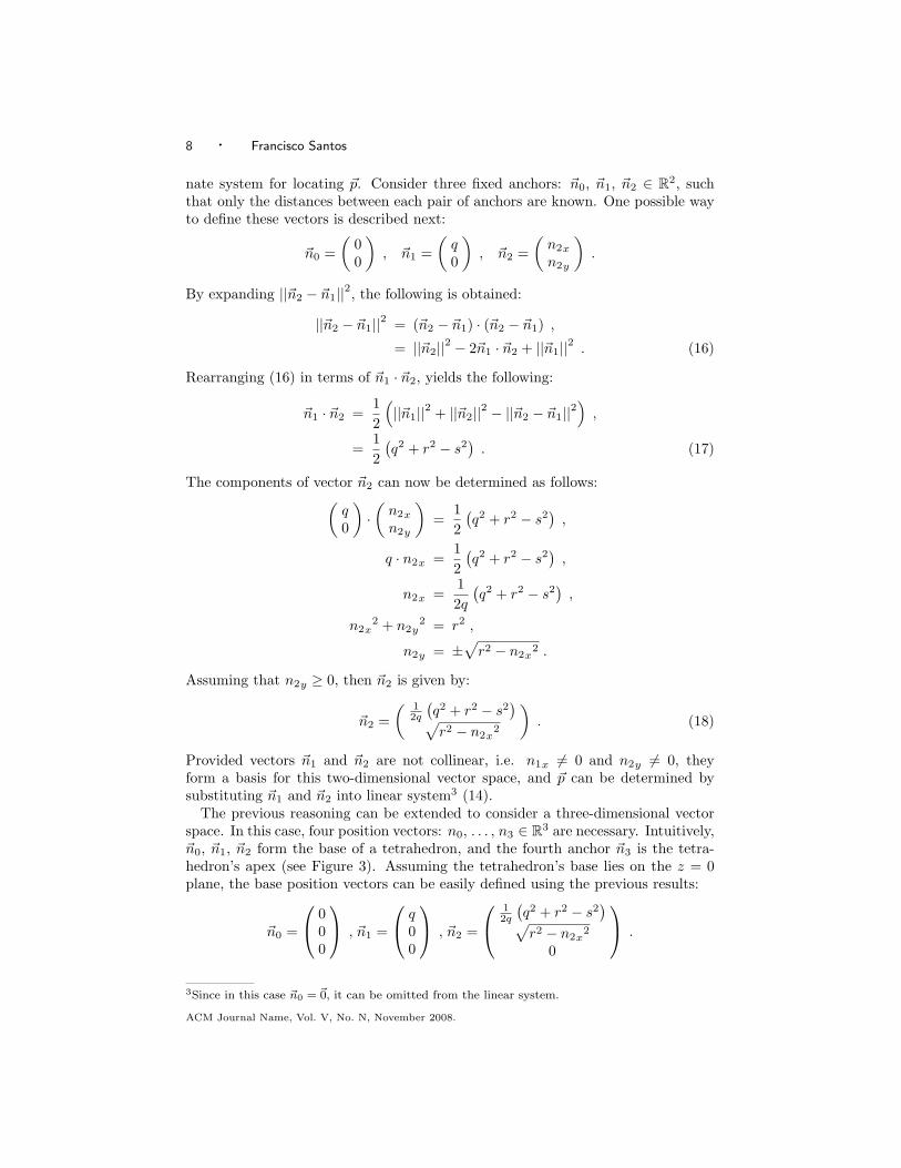
The last two sections described a simple method for computing a node’s positionbased on its distance to the anchor nodes. Triangulation, unlike trilateration,computes the position of a node in space based on the angular distance betweenthree different pairs of anchors, measured from the node. Consider the exampledepicted in Figure 2, where ~p is the node’s position and ~n0, . . . , ~n2 are the anchornodes. If we know the angles between the line segments connecting ~p and the an-chors, but not the segment lengths (i.e. d0, . . . , d2), then the unknown coordinatesmust be found using triangulation instead of trilateration. Fortunately, both tech-niques are very similar and we can adapt the trilateration method to find ~p in thiscase.

Let A0, . . . , A2 denote the angles between the line segments connecting ~p to theanchors, as illustrated in Figure 4. Further, let ~p be the intersection point ofthe three (imaginary) circles centered at ~c0, . . . ,~c2. Knowing the angular distancebetween the anchor nodes, the centers of the circles can be obtained. Consider thecircle centered at ~c0. The major arc (~n1, ~n2) subtends a central angle of 2A0 rad.Hence, the minor arc (~n1, ~n2) subtends a central angle of 2π−2A0 = 2(π−A0) rad.By applying the law of sines to triangle (~n1, ~p, ~n2), the radius of the circumscribedcircle, centered at ~c0, can be found:

rc0 =12||~n1 − ~n2||

sinA0. (30)

The midpoint of line segment (~n1, ~n2) is given by:

~m12 = ~n2 +12

(~n1 − ~n2) . (31)

Position vector ~c0 can be determined by solving the following equation:

(~n1 − ~n2)||~n1 − ~n2||

· R(π/2) =(~c0 − ~m12)||~c0 − ~m12||

forR(π/2) =[

0 1−1 0

](32)

where matrix R(π/2) describes a counterclockwise rotation of π/2 rad. Knowingthat ||~c0 − ~m12|| = rc0 cos(π −A0), (32) can be rewritten with respect to ~c0:

~c0 = ~m12 + rc0 cos(π −A0)(~n1 − ~n2)||~n1 − ~n2||

· R(π/2) (33)



0

21c

Asin

nn

2

1r0

rr−

=

A0

A1

A2

c1

c0

c2

p

n2

n0

n1

A0

m12

Fig. 4. Triangulation.

Similarly, the remaining vectors ~c1 and ~c2 are defined as:

~c1 = ~m02 + rc1 cos(π −A1)(~n0 − ~n2)||~n0 − ~n2||

· R(π/2) , (34)

~c2 = ~m01 + rc2 cos(π −A2)(~n0 − ~n1)||~n0 − ~n1||

· R(π/2) . (35)

Recall that ~p is the intersection point of the circles centered at ~c0, . . . ,~c2. Thisgeometric constraint can be modeled as follows:

||~p− ~ci||2 = r2ci for i = 0, . . . , 2 (36)

Lastly, we can use linear system (14) to find ~p, substituting ~ni with ~ci and di withrci , for i = 0, . . . , 2.

4. LOCALIZATION ALGORITHMS

This Section presents existing algorithms for determining the positions of nodes,based on adaptations of the different distance estimation and localization techniquespresented earlier. The Directionality based Localization Discovery Scheme (DLDS)[Nasipuri and Li 2002] combines signal AoA with triangulation to locate nodes.Wireless stations, equipped with directional antennae, emit continuous RF signalsthat must be within range of all sensor nodes. Nodes then compute the angulardistance between consecutive stations and use triangulation to find their positions.ACM Journal Name, Vol. V, No. N, November 2008.


CONTROLUNIT

Figure 1: An example of a sensor network that in-cludes 4 gateway nodes.

3.1 Network ModelWe assume a sensor network model as depicted in Fig-

ure 1. The network consists of a large number of sensornodes (SN), which are located in random but fixed loca-tions, and a central processing and control unit. The sen-sors take periodic observations to detect the existence of atarget signal in its vicinity (such as temperature, contami-nation level, physical movements, etc.), and transmit a lo-cally processed information to the control unit (CU) whennecessary. Each SN has a processor, memory, and hard-ware that allow limited signal processing, data compression,and wireless networking operations. The SNs have limitedtransmission range. Hence, they rely on store-and-forwardmulti-hop packet transmission for communication. All nodesmaintain multihop routes to one of several gateway nodes inthe network, which have wired links to the CU. The CU isresponsible for taking the final decision on the existence ofa target signal and determining the its location based onthe observations sent by the sensors and other geographicalinformation. To achieve scalability, the sensor network maybe designed such that the SNs cooperate and combine theirobservations locally before sending any message through thenetwork to the CU. It must be noted that the actual func-tioning of the networking operations is not a direct concernin this work. We describe the network model for the readerto visualize the application scenario where the localizationprinciple is applied.

3.2 Beacon signal generationWe assume the presence of at least three fixed wireless

transmission stations or beacon nodes in the network. Thesenodes are equipped with special transmission capabilities forsending wireless beacon signals throughout the sensor net-work. The beacon signals are designed to enable any sensornode to determine its angular bearings with respect to thebeacon nodes. For this purpose, we assume that each beaconsignal consists of a continuous RF carrier signal on a nar-row directional beam that rotates with a constant angularspeed of ω degrees/s. The locations of the beacon nodes canbe arbitrary. For illustration, we assume a rectangular net-work area, with four beacon nodes denoted by BN-1, BN-2,BN-3, and BN-4 placed in the four corners of the networkand co-located with the gateway nodes, as shown in Fig-

BN-3

L

M

(0,0) (L,0)

(Xp,Yp)

(0,M)

BN-1

BN-4

BN-2

α

β

γ

ϕ

3ϕ 2ϕ SN

ω

ω

ω ω

X Y

Z

(L,M)

δ

Figure 2: The model of rotating directional beaconsignals from 4 beacon nodes: BN-1, BN-2, BN-3,and BN-4, located on the corners of the sensor net-work area. The figure shows a test sensor node SNwith its angular bearings with respect to the fourbeacon nodes.

ure 2. The transmissions from different beacon nodes mustbe distinguishable, which may be achieved by using uniqueRF carrier frequencies for each beacon. It may also be im-plemented by using different signature sequences or codeson the same carrier frequency. There is a constant angularseparation of φ degrees between the directional beams fromthe four beacon nodes BN-1, BN-2, BN-3, and BN-4, (seeFigure 2) where φ can be any value. Since all beacons nodesare wired and controlled by the central controller, it is possi-ble to achieve phase synchronization and maintain identicalangular speeds in all of them, which is a requirement for thefunctioning of the proposed localization principle. A rotat-ing directional beam may be implemented by a directionalantenna that is mechanically rotated as done in a radar sys-tem, or it could be generated by an electronically steerablesmart antenna [6]. We assume that the transmission range issufficient for the beacon signals to be received by all sensornodes in the network. Consequently, each sensor node willreceive periodic bursts of the four beacon signals, all withthe same period of 360/ω seconds. However, periodic burstsfrom different beacons will be staggered in time by amountsthat depend on the location of the sensor node.

4. LOCALIZATION PRINCIPLEThe localization principle is based on a sensor node noting

the times when it receives the different beacon signals, andevaluating its angular bearings and location with respectto the beacon nodes by triangulation. Denote the times atwhich an SN receives the beacons signals from BN-1, BN-2,BN-3, and BN-4 by t1, t2, t3, and t4, respectively. Since thesensor nodes have no time synchronization with the beaconnodes, the absolute values of these times bear no useful in-formation. However, the time difference of arrivals can be

107

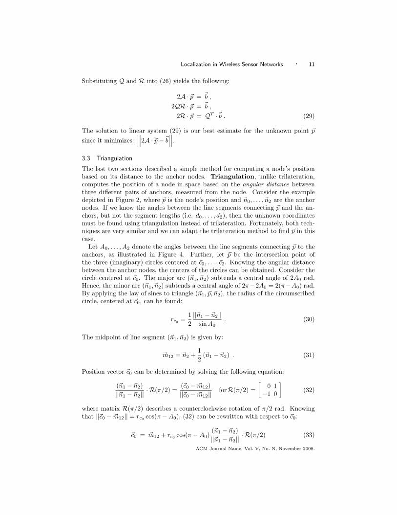
Fig. 5. The model of rotating directional beacon signals from 4 beacon nodes: BN-1, BN-2, BN-3,and BN-4 [Nasipuri and Li 2002].

In TERRAIN and Hop-TERRAIN [Savarese 2002], anchors may be scatteredthroughout the sensor field and do not need to be within range of every sensor node.Both rely on RSS distance estimates and trilateration to locate nodes. According tothe authors [Savarese 2002], TERRAIN allows erroneous distance estimates to prop-agate throughout the network and is too inaccurate to be useful. Hop-TERRAINtakes extra care to ensure that only reliable measurements permeate the network,making it more accurate than TERRAIN. The aforementioned algorithms will beanalyzed in the following subsections.

4.1 Directionality based Location Discovery

The Directionality based Location Discovery Scheme [Nasipuri and Li 2002] isan AoA-based algorithm for performing node localization. This location discov-ery scheme requires at least three fixed wireless transmission stations or beaconnodes, equipped with directional antennae. Sensor nodes use the directional signalsemitted by these stations to determine the angular separation between consecutivebeacon nodes. For this purpose, it is assumed that each beacon signal consists of acontinuous RF carrier signal, detectable by all nodes within the WSN deploymentarea, transmitted in a narrow directional beam, and that rotates with a constant an-gular speed of: ω rad s−1. There is a constant angular separation of φ rad betweenconsecutive beacon nodes: BN-1, BN-2, BN-3, and BN-4 (see Figure 5). Using acentral controller, it is possible to achieve phase synchronization and maintain aconstant angular speed for the beacon signals.

By knowing the arrival time of the different beacon signals, node SN is capableof determining angles: α, β, and δ. Let T1 and T2 be defined as the times at whichSN receives the signals from beacons BN-1 and BN-2, respectively. At time T2, SNhas received BN-2’s signal but BN-1’s signal must still rotate another (T1 − T2)ωrad to reach SN. Rotating BN-1’s signal by φ rad counter-clockwise would make itparallel to that of beacon BN-2. Hence, angle α is given by:

α = (T1 − T2)ω + φ . (37)ACM Journal Name, Vol. V, No. N, November 2008.


By applying a similar reasoning, the remaining angles can be found:

β = (T2 − T3)ω + φ , (38)δ = (T3 − T4)ω + φ , (39)

where T3 and T4 are the arrival times of BN-3 and BN-4’s signals at node SN. Usingtriangulation, the 2D coordinates of node SN can be calculated (see Section 3.3).

Since each node finds its position individually, the performance of this method isunaffected by the WSN’s density. Additionally, since it depends on angle estimates,its performance does not depend on the network’s size. However, there are severalcauses of error for this particular localization scheme. Each signal beacon has anon-zero width, which makes it difficult for nodes to record the precise arrival timeof the signal. According to simulation results, for beam widths of π/12 rad or lessand for a square WSN deployment with a side-length of 75m, the node positionestimates are within ±2m of the real positions [Nasipuri and Li 2002]. Reflectionsfrom surrounding objects are an additional source of error, causing beacon signalsto be received at the sensor nodes even when they are not directed toward them.In this case, simulation results suggest positioning errors greater than ±50m arepossible [Nasipuri and Li 2002], making DLDS an inviable option in the presence ofmultipath interference. Other drawbacks of this algorithm include: the requirementof expensive directional antennae for the beacon nodes, a centralized infra-structureto control beam synchronization, and the limitation on network size imposed bythe finite range of the beacon signals.

4.2 TERRAIN

The Triangulation via Extended Range and Redundant Association of IntermediateNodes (TERRAIN) [Savarese 2002] is an algorithm for performing node localization.The anchors, which have access to precise positioning information, need not bedirectly connected to the other nodes for TERRAIN to operate. For locating anode in three-dimensional space, at least four anchors are required (see Section 3.1),although they may be randomly placed within the network deployment area.

TERRAIN is initiated at the anchor nodes. Each anchor waits for three regularnodes to connect. Knowing the distances between the anchor and each of the regu-lar nodes, and the pairwise distances of the three nodes, it is possible to construct alocal coordinate system, as was explained at the end of Section 3.1. A fourth nodemay determine its position in this coordinate system by performing trilateration,using the relative positions of the three initial nodes. Since the anchor is located atthe origin, the norm of the fourth node’s position vector will equal the distance tothat anchor. Nodes which have determined their positions relative to a particularanchor, broadcast this information to the rest of the network. Through multilat-eration (see Section 3.2), other nodes determine their positions relative to eachof the existing anchor nodes. By calculating the norm of these position vectors,the distance to each anchor is thus found. Knowing the anchors’ global positions,and the distance to each anchor, a node is able to find its global position throughmultilateration.

This algorithm relies on the RSS technique for estimating distances betweennodes. However, RSS-based distance estimates are unreliable. As nodes performACM Journal Name, Vol. V, No. N, November 2008.


1

2

3 4

4' 5

anchor node

regular node

Fig. 6. Example of a 2D hard-topology: node 4 does not have a uniquely determined position

[Savarese 2002].

multilateration based on incorrect position vectors, the errors may accumulate andaffect future calculations. According to the authors [Savarese 2002], the final posi-tion estimates are too far from the true positions to be useful.

4.3 Hop-TERRAIN

Unlike TERRAIN, the Hop-TERRAIN [Savarese 2002] algorithm does not use theRSS values directly to estimate distances to the anchor nodes (see Section 4.2).In this algorithm, nodes determine the minimum hop-count to the anchors andthen multiply this by the average distance per hop measure. This value may bepre-configured, or calculated at runtime by the anchor nodes and then broadcastto the remainder of the network. Hop-TERRAIN operates in two phases: start-upand refinement. A crude initial position estimate is calculated during the start-upphase, which is later improved during refinement.

In the start-up phase, the anchor nodes flood the network with positioning pack-ets, containing their locations and a hop-count field initially set to zero. Uponreceiving a positioning packet, a node records the anchor’s position, incrementsand stores the hop-count value, computes the distance to the anchor node, and,finally, re-broadcasts the packet. To avoid unnecessary broadcasts, a node onlyaccepts a new positioning packet if it refers to a new anchor, or the hop-count to anexisting anchor is lower than the previously recorded value. Knowing the positionsand distances to at least four different anchors, a node is able to find its positionin three-dimensional space using multilateration. After making the initial positionestimate, the node may enter the refinement phase.

Refinement is an iterative algorithm for improving the nodes’ initial position es-timates. At the beginning of each step, a node broadcasts its position and listensfor the positioning packets of its direct neighbors. Using the estimated distances toits one-hop neighbors and their respective locations, the node re-calculates its ownposition using multilateration, and broadcasts the result. Nodes end the refinementphase when their updated positions are sufficiently close to their previous estimates,or when a pre-configured maximum number of iterations is reached. The study ofthe refinement algorithm revealed two main problems [Basagni et al. 2004][Savarese2002]: (i) error propagation through the network due to unreliable position esti-mates, and (ii) failure when applied to hard topologies, where parts of a networkcan be mirrored while preserving inter-node ranges (see Figure 6).

To minimize the effects of an erroneous position estimate on the remaining calcu-ACM Journal Name, Vol. V, No. N, November 2008.


1

2

4 856

7

3

anchor node

regular node

Fig. 7. Example of a 2D hard-topology where the heuristic, defined in [Savarese 2002], fails.

lations, weights reflecting the confidence of each estimate are used [Savarese 2002].Confidence levels range between 0 and 1. Anchors are assigned a value of 1, andnodes that enter the refinement phase are assigned a confidence of 0.1. Each timea node successfully performs multilateration, it updates its confidence level to theaverage confidence levels of its neighbors. If multilateration fails due to insufficientconstraints or because other consistency criteria where not met, confidence is setto 0 to avoid propagating inaccurate data. A node is excluded from refinement ifit persistently fails to provide consistent results. The simulation results note thatalthough the use of confidence levels yields an improvement on the average errorin computed results, it cannot be used as an indicator of the estimated accuracy[Basagni et al. 2004].

A network with a hard-topology can be partially reflected while maintainingthe distances between nodes. For example, node 4 in Figure 6 has two possiblepositions that are consistent with the distance measurements. In such a case, onlythose nodes that have edge-disjoint paths to at least four anchors (or three fortwo dimensional scenarios) are capable of determining their positions [Willig 2006].Such nodes are called sound. The authors propose a heuristic that can filter-outmost non-sound nodes [Savarese 2002]. During the start-up phase, nodes record theID of the next-hop neighbor along the shortest path to a given anchor. When thenumber of unique neighbor IDs recorded reaches four (or three for two dimensionalscenarios), the node declares itself sound, and enters the refinement phase. Theneighbors then record the sound node’s ID, and the process continues around thenetwork.

The hard-topology heuristic described in [Savarese 2002] can sometimes fail. Allnodes in Figure 7 can reach the three anchors, and, hence, proceed to refinement.The information stored in each node at the end of the start-up phase is presentedin Table I (the anchor positions are not shown for brevity). Nodes 6 and 7 arecorrectly marked not-sound by Hop-TERRAIN, since both nodes can have twovalid positions while still obeying inter-node ranges. Node 8 can have only oneposition. Either of the two possible physical locations for 6 and 7 can be used innode 8’s trilateration, together with node 3’s position. Hop-TERRAIN will onlymark node 8 sound if the next-hop neighbor along the path to anchor 1 is differentthan that of anchor 2, which is the only case when the size of the neighbor ID set isequal to three. Node 5 can compute its location by trilaterating node 4’s positionACM Journal Name, Vol. V, No. N, November 2008.


Table I. Hop-TERRAIN start-up tables for the example in Figure 7.

Node 4

Anchor Next-hop Hop-count

1 1 1

2 2 1

3 5 4

Neighbor IDs: {1, 2, 5}

Node 5


1 4 2

2 4 2

3 6 or 7a 4

Neighbor IDs: {4, 6} or {4, 7}

Node 6


1 5 3

2 5 3

3 8 2

Neighbor IDs: {5, 8}

Node 7


1 5 3

2 5 3

3 8 2

Neighbor IDs: {5, 8}

Node 8


1 6 or 7 3

2 6 or 7 3

3 3 1

Neighbor IDs: {3, 6} or {3, 7} or {3, 6, 7}b

(a) – Depends on the route taken by anchor 2’s positioning packet.

(b) – Route taken by a positioning packet can affect the “soundness” of a node.

and the real or reflected positions for node’s 6 and 7. However, Hop-TERRAINmistakenly considers 5 a non-sound node since its neighbor set does not containthree unique IDs. Finally, node 4 is correctly marked sound, as it can find itsposition by trilaterating the positions of nodes 1, 2, and 5.

According to the simulation results, the Hop-TERRAIN algorithm achieves, onaverage, position errors of less than 33% of a node’s radio range in the presence ofa 5% range measurement error, when at least 5% of the nodes are anchors [Basagniet al. 2004].

5. CONCLUSION

Current papers on positioning systems for WSNs typically focus on the isolatedparts of the localization process, concentrating on: methods for estimating inter-node ranges and angles, mathematical techniques for determining the position ofa single node, and algorithms for computing the positions of nodes in an entireWSN. This paper aims to dissect the node localization procedure, explaining itsindividual phases, and to analyze existing positioning systems for sensor networks,describing their major benefits and flaws.

The localization task for WSNs is divided into three main phases. A node startsby finding the ranges or angular separation between nodes with pre-calculated co-ordinates, known as anchors. Knowing the ranges to three distinct anchors, a nodeperforms trilateration to find its 2D position. Alternatively, it can triangulate its2D position using the angular distance between three different pairs of anchors.



Lastly, a node must forward its position so that other nodes can calculate theircoordinates. The more successful localization algorithms take additional steps toachieve positioning accuracy by preventing the propagation of calculation errors.

Depending on the hardware available at each node, different distance and angleestimation strategies can be used. The RSS strategy uses the voltage of the radiotransceiver’s RSSI circuit as an indicator of distance, requiring no dedicated net-work packets to operate. Unfortunately, the RSS ranging technique is error proneand is disfavored when accuracy is a priority. One alternative method computes theinter-node range by measuring the time-of-flight of a signal with a known propaga-tion velocity. This method requires high-precision clocks and tight synchronizationbetween sender and receiver to yield accurate results. As opposed to measuringinter-node distances, nodes may opt to estimate the angular separation betweenpairs of anchors, at the cost of extra hardware.

To illustrate the more theoretical concepts introduced in this article, three ex-isting localization algorithms were analyzed. The Directionality based LocalizationDiscovery Scheme combines signal AoA with triangulation to locate nodes. Sinceeach node performs triangulation independently, the performance of DLDS is un-affected by the WSN’s density. One major drawback of this algorithm is its intol-erance to multipath interference, yielding positioning errors of ±50m for a squareWSN with a side length of 75m. Unlike DLDS, the TERRAIN and Hop-TERRAINalgorithms do not require anchors to be within range of the regular nodes. Bothalgorithms use RSS-based distance estimates and triangulation to find nodal po-sitions. While TERRAIN is too inaccurate to be useful, Hop-TERRAIN takesserious measures to contain calculation errors. According to simulation results,Hop-TERRAIN achieves, on average, position errors of less than 33% of a node’sradio range in the presence of a 5% range measurement error, when at least 5% ofthe nodes are anchors.

ACKNOWLEDGMENTS

The author wishes to thank Prof. Jose Luıs Fachada for his insightful help in pre-senting the mathematical concepts underlying localization and to all contributorswhose suggestions and feedback have improved this work.

REFERENCES

Basagni, S., Conti, M., Giordano, S., and Stojmenovic, I. 2004. Mobile Ad-hoc Networking.

John Wiley & Sons.

Bonnet, P., Gehrke, J., and Seshadri, P. 2001. Towards Sensor Database Systems. In

MDM 2001: Proceedings of the Second International Conference on Mobile Data Management.Springer-Verlag, London, UK, 3–14.

Fang, B. 1986. Trilateration and Extension to Global Positioning System Navigation. Journalof Guidance, Control, and Dynamics 9, 715–717.

Fok, C.-L., Roman, G.-C., and Lu, C. 2005. Mobile agent middleware for sensor networks:

an application case study. In IPSN 2005: Proceedings of the 4th international symposium onInformation processing in sensor networks. IEEE Press, Piscataway, NJ, USA, 382–387.

Heidemann, J., Silva, F., Intanagonwiwat, C., Govindan, R., Estrin, D., and Ganesan,

D. 2001. Building efficient wireless sensor networks with low-level naming. In SOSP 2001:

Proceedings of the eighteenth ACM symposium on Operating systems principles. ACM, NewYork, NY, USA, 146–159.



Karl, H. and Willig, A. 2005. Protocols and Architectures for Wireless Sensor Networks. John

Wiley and Sons, The Atrium, Southern Gate, Chichester, West Sussex PO19 8SQ, England.

Karp, B. and Kung, H. T. 2000. GPSR: Greedy Perimeter Stateless Routing for WirelessNetworks. In MobiCom 2000: Proceedings of the 6th Annual International Conference on

Mobile Computing and Networking. ACM Press, New York, NY, USA, 243–254.

Magalhaes, L. 1989. Algebra Linear como Introducao a Matematica Aplicada. Texto Editora.

McCrady, D., Doyle, L., Forstrom, H., Dempsey, T., and Martorana, M. 2000. Mobile rang-ing using low-accuracy clocks. IEEE Transactions on Microwave Theory and Techniques 48, 6

(June), 951–958.

Nasipuri, A. and Li, K. 2002. A Directionality Based Location Discovery Scheme for Wireless

Sensor Networks. In WSNA 2002: Proceedings of the 1st ACM International Workshop onWireless Sensor Networks and Applications. ACM Press, New York, NY, USA, 105–111.

Ottersten, B., Viberg, M., Stoica, P., and Nehorai, A. 1993. Exact and large sample ML

techniques for parameter estimation and detection in array processing. In Radar Array Pro-cessing – Chapter 4. Springer-Verlag New York, Inc., Secaucus, NJ, USA, 99–151.

Patwari, N., Ash, J., Kyperountas, S., III, A. H., Moses, R., and Correal, N. July 2005.

Locating the nodes: cooperative localization in wireless sensor networks. Signal Processing

Magazine, IEEE 22, 4, 54–69.

Savarese, C. 2002. Robust Positioning Algorithms for Distributed Ad-hoc Wireless Sensor Net-

works. M.S. thesis, Department of Electrical Engineering and Computer Sciences, University

of California.

Steingart, D., Wilson, J., Redfern, A., Wright, P., Romero, R., and Lim, L. 2005. Aug-mented Cognition for Fire Emergency Response: An Iterative User Study. In Proceedings of

the 1st International Conference on Augmented Cognition. Las Vegas, NV.

Stoica, P. and Moses, R. 1997. Introduction to Spectral Analysis, 1st ed. Prentice Hall, Inc.,Upper Saddle River, NJ 07458, USA.

Willig, A. 2006. Wireless Sensor Networks: Concept, Challenges and Approaches. In e & i

Elektrotechnik und Informationstechnik. Vol. 123. Springer Wien, 224–231.

Received Month Year; revised Month Year; accepted Month Year


Documents

Localization in Wireless Sensor Networks - ULisboaweb.ist.utl.pt/ist150077/doc/localization.pdf · Localization in Wireless Sensor Networks ... In wireless sensor networks (WSNs),