TVP-VARs and Factor Models

() TVP-VARs 1 / 49

Introduction

Why TVP-VARs?

Example: U.S. monetary policy

was the high inflation and slow growth of the 1970s were due to badpolicy or bad luck?

Some have argued that the way the Fed reacted to inflation haschanged over time

After 1980, Fed became more aggressive in fighting inflation pressuresthan before

This is the “bad policy” story (change in the monetary policytransmission mechanism)

This story depends on having VAR coeffi cients different in the 1970sthan subsequently.

() TVP-VARs 2 / 49

Others think that variance of the exogenous shocks hitting economyhas changed over time

Perhaps this may explain apparent changes in monetary policy.

This is the “bad luck” story (i.e. 1970s volatility was high, adverseshocks hit economy, whereas later policymakers had the good fortuneof the Great Moderation of the business cycle —at least until 2008)

This motivates need for multivariate stochastic volatility to VARmodels

Cannot check whether volatility has been changing with ahomoskedastic model

() TVP-VARs 3 / 49

Most macroeconomic applications of interest involve several variables(so need multivariate model like VAR)

Also need VAR coeffi cients changing

Also need multivariate stochastic volatility

TVP-VARs are most popular models with such features

But other exist (Markov-switching VARs, Vector Floor and CeilingModel, etc.)

() TVP-VARs 4 / 49

Homoskedastic TVP-VARs

Begin by assuming Σt = ΣRemember VAR notation: yt is M × 1 vector, Zt is M × k matrix(defined so as to allow for a VAR with different lagged dependent andexogenous variables in each equation).

TVP-VAR:yt = Ztβt + εt

βt+1 = βt + ut

εt is i.i.d. N (0,Σ) and ut is i.i.d. N (0,Q).εt and us are independent of one another for all s and t.

() TVP-VARs 5 / 49

Bayesian inference in this model?

Already done: this is just the Normal linear state space model of thelast lecture.

MCMC algorithm of standard form (e.g. Carter and Kohn, 1994).

But let us see how it works in practice in our empirical application

Follow Primiceri (2005)

() TVP-VARs 6 / 49

Illustration of Bayesian TVP-VAR Methods

Same quarterly US data set from 1953Q1 to 2006Q3 as was used toillustrate VAR methods

Three variables: Inflation rate ∆πt , the unemployment rate ut andthe interest rate rtVAR lag length is 2.

Training sample prior: prior hyperparameters are set to OLS quantitiescalculating using an initial part of the data

Our training sample contains 40 observations.

Data through 1962Q4 used to choose prior hyperparameter values,then Bayesian estimation uses data beginning in 1963Q1.

() TVP-VARs 7 / 49

βOLS is OLS estimate of VAR coeffi cients in constant-coeffi cient VARusing training sample

V (βOLS ) is estimated covariance of βOLS .

Prior for β0:β0 ∼ N (βOLS , 4 · V (βOLS ))

Prior for Σ−1 Wishart prior with ν = M + 1, S = I

Prior for Q−1 Wishart prior with νQ = 40,Q = 0.0001 · 40 · V (βOLS )

() TVP-VARs 8 / 49

With TVP-VAR we have different set of VAR coeffi cients in everytime period

So different impulse responses in every time period.

Figure 1 presents impulse responses to a monetary policy shock inthree time periods: 1975Q1, 1981Q3 and 1996Q1.

Impulse responses defined in same way as we did for VAR

Posterior median is solid line and dotted lines are 10th and 90th

percentiles.

() TVP-VARs 9 / 49

Figure 1: Impulse responses at different times() TVP-VARs 10 / 49

Combining other Priors with the TVP Prior

Often Bayesian TVP-VARs work very well in practice.

In some case the basic TVP-VAR does not work as well, due toover-parameterization problems.

Previously, we noted worries about proliferation of parameters inVARs, which led to use of priors such as the Minnesota prior or theSSVS prior.

With many parameters and short macroeconomic time series, it canbe hard to obtain precise estimates of coeffi cients.

Risk of over-fitting

Priors which exhibit shrinkage of various sorts can help mitigate theseproblems.

With TVP-VAR proliferation of parameters problems is even moresevere.

Hierarchical prior of state equation is big help, but may want more insome cases.

() TVP-VARs 11 / 49

Combining TVP Prior with Minnesota Prior

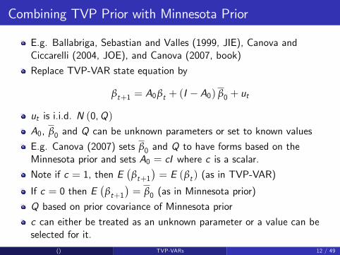
E.g. Ballabriga, Sebastian and Valles (1999, JIE), Canova andCiccarelli (2004, JOE), and Canova (2007, book)

Replace TVP-VAR state equation by

βt+1 = A0βt + (I − A0) β0 + ut

ut is i.i.d. N (0,Q)

A0, β0 and Q can be unknown parameters or set to known values

E.g. Canova (2007) sets β0 and Q to have forms based on theMinnesota prior and sets A0 = cI where c is a scalar.

Note if c = 1, then E(

βt+1)= E (βt ) (as in TVP-VAR)

If c = 0 then E(

βt+1)= β0 (as in Minnesota prior)

Q based on prior covariance of Minnesota prior

c can either be treated as an unknown parameter or a value can beselected for it.

() TVP-VARs 12 / 49

Combining TVP Prior with SSVS Prior

Same setup as preceding slide

Set β0 = 0.

Let a0 = vec (A0)

Use SSVS prior for a0a0j (the j th element of a0) has prior:

a0j |γj ∼(1− γj

)N(0, κ20j

)+ γjN

(0, κ21j

)as before, γj is dummy variable

κ20j is very small (so that a0j is constrained to be virtually zero)

κ21j is large (so that a0j is relatively unconstrained).

Property: with probability γj , a0j is evolving according to a randomwalk in the usual TVP fashion

With probability(1− γj

), a0j ≈ 0

() TVP-VARs 13 / 49

MCMC Algorithm

I will not provide complete details, but note only:

These are Normal linear state space models so standard algorithms(e.g. Carter and Kohn) can draw βT

For TVP+Minnesota prior this is enough (other parameters fixed)

For TVP+SSVS simple to adapt MCMC algorithm for SSVS withVAR

() TVP-VARs 14 / 49

Adding Another Layer to the Prior Hierarchy

Another approach used by Chib and Greenberg (1995, JOE) for SURmodel

Adapted for VARs by, e.g., Ciccarelli and Rebucci (2002)

yt = Ztβt + εt

βt+1 = A0θt+1 + utθt+1 = θt + ηt

all assumptions as for TVP-VAR, plus ηt is i.i.d. N (0,R)

Slightly more general that previous Normal linear state space model,but very similar MCMC (so will not discuss MCMC)

() TVP-VARs 15 / 49

Adding Another Layer to the Prior Hierarchy

Why might this generalization be useful?

A0 can be chosen to reflect some other prior information

E.g. SSVS prior as above

E.g. Ciccarelli and Rebucci (2002) is panel VAR application

G countries and, for each country, kG explanatory variables exist withtime-varying coeffi cients.

They setA0 = ιG ⊗ IkG

Implies time-varying component in each coeffi cient which is commonto all countries

Parsimony: θt is of dimension kG whereas βt is of dimension kG × G .

() TVP-VARs 16 / 49

Imposing Inequality Restrictions on the VAR Coeffi cients

Another way of ensuring shrinkage

E.g. restrict βt to be non-explosive (i.e. roots of the VAR polynomialdefined by βt lie outside the unit circle)

Sometimes (given over-fitting and imprecise estimates) can getposterior weight in explosive region

Even small amount of posterior probability in explosive regions for βtcan lead to impulse responses or forecasts which havecounter-intuitively large posterior means or standard deviations.

Koop and Potter (2009, on my website) discusses how to do this. Iwill not present details, but outline basic idea

() TVP-VARs 17 / 49

With unrestricted TVP-VAR, took draws p(

βT |yT ,Σ,Q)using

MCMC methods for Normal linear state space models

One method to impose inequality restrictions involves:

Draw βT in the unrestricted VAR. If any drawn βt violates theinequality restriction then the entire vector βT is rejected.

Problem: this algorithm can get stuck, rejecting virtually every βT

(all you need is a single drawn βt to violate inequality and entire βT

is rejected)

Note: algorithms like Carter and Kohn are “multi-move algorithms”(draw βT all at same time).

Alternative is “single move algorithm”: drawing βt for t = 1, ..,T oneat a time from p

(βt |yT ,Σ,Q, β−t

)where

β−t =(

β′1, .., βt−1, βt+1, .., β′T

)′

() TVP-VARs 18 / 49

Koop and Potter (2009) suggest using single move algorithm

Reject βt only (not βT ) if it violates inequality restriction

Usually multi-move algorithms are better than single-move algorithmssince latter can be slow to mix.

I.e. they produce highly correlated series of draws which means that,relative to multi-move algorithms, more draws must be taken toachieve a desired level of accuracy.

But if multi-move algorithm gets stuck, single move might be better.

() TVP-VARs 19 / 49

Dynamic Mixture Models

Remember: Normal linear state space model depends on so-calledsystem matrices, Zt , Qt , Tt , Wt and Σt .Suppose some or all of them depend on an s × 1 vector K̃tSuppose K̃t is Markov random variable (i.e.

p(K̃t |K̃t−1, .., K̃1

)= p

(K̃t |K̃t−1

)or independent over t

Particularly simple if K̃t is a discrete random variable.

Result is called a dynamic mixture model

Gerlach, Carter and Kohn (2000, JASA) have an effi cient MCMCalgorithm

() TVP-VARs 20 / 49

Why are dynamic mixture models useful in empirical macroeconomics?

E.g. TVP-VAR:yt = Ztβt + εt

βt+1 = βt + ut

εt is i.i.d. N (0,Σ)

BUT: ut is i.i.d. N(0, K̃tQ

).

Let K̃t ∈ {0, 1} with hierarchical prior:

p(K̃t = 1

)= q.

p(K̃t = 0

)= 1− q

where q is an unknown parameter.

() TVP-VARs 21 / 49

Property:

If K̃t = 1 then usual TVP-VAR:

βt+1 = βt + ut

If K̃t = 0 then VAR coeffi cients do not change at time t:

βt+1 = βt

Parsimony.

This model can have flexibility of TVP-VAR if the data warrant it(i.e. can select K̃t = 1 for t = 1, ..,T ).

But can also select a much more parsimonious representation.

An extreme case: if K̃t = 0 for t = 1, ..,T then back to VAR withouttime-varying parameters.

() TVP-VARs 22 / 49

I will not present details of MCMC algorithm since it is becoming astandard one

See also the Matlab code on my website

Dynamic mixture models used to model structural breaks, outliers,nonlinearities, etc.

E.g. Giordani, Kohn and van Dijk (2007, JoE).

() TVP-VARs 23 / 49

TVP-VARs with Stochastic Volatility

In empirical work, you will usually want to add multivariate stochasticvolatility to the TVP-VAR

But this can be dealt with quickly, since the appropriate algorithmswere described in the lecture on State Space Modelling

Remember, in particular, the approaches of Cogley and Sargent(2005) and Primiceri (2005).

MCMC: need only add another block to our algorithm to draw Σt fort = 1, ..,T .

Homoskedastic TVP-VAR MCMC: p(Q−1|yT , βT

),

p(

βT |yT ,Σ,Q)and p

(Σ−1|yT , βT

)Heteroskedastic TVP-VAR MCMC: p

(Q−1|yT , βT

),

p(

βT |yT ,Σ1, ..,ΣT ,Q)and p

(Σ−11 , ..,Σ

−1T |yT , β

T)

() TVP-VARs 24 / 49

Empirical Illustration of Bayesian Inference in TVP-VARswith Stochastic Volatility

Continue same illustration as before.

All details as for homoskedastic TVP—VAR

Plus allow for multivariate stochastic volatility as in Primiceri (2005).

Priors as in Primiceri

Can present empirical features of interest such as impulse responses

But (for brevity) just present volatility information

Figure 2: time-varying standard deviations of the errors in the threeequations (i.e. the posterior means of the square roots of the diagonalelement of Σt)

() TVP-VARs 25 / 49

Figure 2: Volatilities in the 3 Equations() TVP-VARs 26 / 49

Summary of TVP-VARs

TVP-VARs are useful for the empirical macroeconomists since they:

are multivariate

allow for VAR coeffi cients to change

allow for error variances to change

They are state space models so Bayesian inference can use familiarMCMC algorithms developed for state space models.

They can be over-parameterized so care should be taken with priors.

Recently there has been interest in large TVP-VARs

() TVP-VARs 27 / 49

Factor Methods

In past VARs and TVP-VAR usually have small number of dependentvariables (e.g. 3 or 4 and rarely more than 10)

Increasingly researchers working with large VARs (and even largeTVP-VARs)

But before large VARs, factor methods were dominant answer toquestion:

How to extract information in data sets with many variables but keepmodel parsimonious?

() TVP-VARs 28 / 49

Static Factor Model

yt is M × 1 vector of time series variablesM is very large

yit denote a particular variable.

Simplest static factor model:

yt = λ0 + λft + εt

ft is q × 1 vector of unobserved latent factors (where q << M)Factors contain information extracted from all the M variables.

Same ft occurs in every equation for yit for i = 1, ...,M

But different coeffi cients (λ is an M × q matrix of so-called factorloadings).

() TVP-VARs 29 / 49

Note that restrictions are necessary to identify the model

Common to say εt is i.i.d. N (0,D) where D is diagonal matrix.

Implication: εit is pure random shock specific to variable i ,co-movements in the different variables in yt arise only from thefactors.

Note also that λft = λCC−1ft which shows we need identificationrestriction for factors too.

Different models arise from different treatment of factors.

Simplest is: ft ∼ N (0, I )This can be interpreted as a state equation for “states” ftFactor models are state space models – so our MCMC tools ofLecture 3 can be used.

() TVP-VARs 30 / 49

The Dynamic Factor Model (DFM)

In macroeconomics, usually need to extend static factor model toallow for the dynamic properties which characterize macroeconomicvariables.

A typical DFM:

yit = λ0i + λi ft + εitft = Φ1ft−1 + ..+Φp ft−p + εft

ft is as for static model

λi is 1× q vector of factor loadings.Each equation has its own intercept, λ0i .

εit is i.i.d. N(0, σ2i

)ft is VAR with εft being i.i.d. N

(0,Σf

)Note: usually εit is autocorrelated (easy extension, omitted here forsimplicity)

() TVP-VARs 31 / 49

Replacing Factors by Estimates: Principal Components

Proper Bayesian analysis of the DFM treats ft as vector of unobservedlatent variables.

Before doing this, we note a simple approximation.

The DFM has similar structure to regression model:

yit = λ0i + λ̃0i ft + ..+ λ̃pi ft−p + ε̃it

If ft were known we could use Bayesian methods for the multivariateNormal regression model to estimate or forecast with the DFM.

Principal components methods to can be used to approximate ft .

Precise details of how principal components is done provided manyplaces

() TVP-VARs 32 / 49

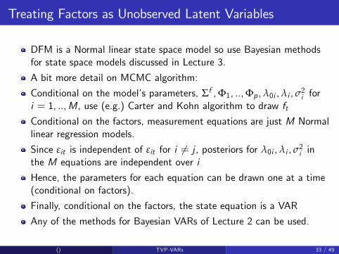
Treating Factors as Unobserved Latent Variables

DFM is a Normal linear state space model so use Bayesian methodsfor state space models discussed in Lecture 3.

A bit more detail on MCMC algorithm:

Conditional on the model’s parameters, Σf ,Φ1, ..,Φp ,λ0i ,λi , σ2i for

i = 1, ..,M, use (e.g.) Carter and Kohn algorithm to draw ftConditional on the factors, measurement equations are just M Normallinear regression models.

Since εit is independent of εit for i 6= j , posteriors for λ0i ,λi , σ2i in

the M equations are independent over i

Hence, the parameters for each equation can be drawn one at a time(conditional on factors).

Finally, conditional on the factors, the state equation is a VAR

Any of the methods for Bayesian VARs of Lecture 2 can be used.

() TVP-VARs 33 / 49

The Factor Augmented VAR (FAVAR)

DFMs are good for forecasting (extract all information in hugenumber of variables)

VARs are good for macroeconomic policy (e.g. impulse responses).

Why not combine DFMs and VARs together to get model which cando both?

FAVAR results

Bernanke, Boivin and Eliasz (2005, QJE) is pioneering paper

() TVP-VARs 34 / 49

Impulse Response Analysis in DFM

With VARs impulse responses based on structural VAR:

C0yt = c0 +p

∑j=1Cjyt−j + ut

ut is i.i.d. N (0, I ) and C0 chosen to give shocks structuralinterpretationIf C (L) = C0 −∑p

j=1 CjLp impulse responses obtained from VMA:

yt = C (L)−1 ut

With the DFM, can obtain VMA representation for yt by substitutingin factor equation:

yt = εt + λΦ (L)−1 εft= B (L) ηt

But ηt combines εt and εft – cannot isolate “shock to interest rateequation”as monetary policy shock and do impulse response analysisin standard way.

() TVP-VARs 35 / 49

FAVAR modifies DFM by adding other explanatory variables:

yit = λ0i + λi ft + γi rt + εit

rt is kr × 1 vector of observed variables of key interest.E.g. Bernanke, Boivin and Eliasz (2005) set rt to be the Fed Fundsrate (a monetary policy instrument)

All other assumptions are same as for the DFM.

Note: by treating rt in this way, we can isolate a “monetary policyshock”and calculate impulse responses

() TVP-VARs 36 / 49

FAVAR state equation extends DFM state equation to include rt :(ftrt

)= Φ̃1

(ft−1rt−1

)+ ..+ Φ̃p

(ft−prt−p

)+ ε̃ft

where all assumptions are same as DFM with extension that ε̃ft is

i.i.d. N(0, Σ̃f

)MCMC is very similar to that for the DFM and will not be describedhere.

Similar ideas:

Normal linear state space algorithms can draw ftMeasurement equation is series of regressions (conditional on factors)

The state equation is a VAR (conditional of factors)

() TVP-VARs 37 / 49

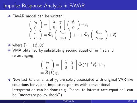
Impulse Response Analysis in FAVAR

FAVAR model can be written:(ytrt

)=

[λ γ0 1

] (ftrt

)+ ε̃t(

ftrt

)= Φ̃1

(ft−1rt−1

)+ ..+ Φ̃p

(ft−prt−p

)+ ε̃ft

where ε̃t = (ε′t , 0)′

VMA obtained by substituting second equation in first andre-arranging (

ytrt

)=

[λ γ0 1

]Φ̃ (L)−1 ε̃ft + ε̃t

= B̃ (L) ηt

Now last kr elements of ηt are solely associated with original VAR-likeequations for rt and impulse responses with conventionalinterpretation can be done (e.g. “shock to interest rate equation”canbe “monetary policy shock”)

() TVP-VARs 38 / 49

The TVP-FAVAR

With VARs: began with constant parameter model

then we said it is good to allow the VAR coeffi cients to vary overtime: homoskedastic TVP-VAR

then we said good to allow for multivariate stochastic volatility:heteroskedastic TVP-VAR

Recent research (e.g. working papers: Del Negro and Otrok (2008,NYFed) and Korobilis (2013, OBES)) is doing the same with FAVARs

Note: just as with TVP-VARs, TVP-FAVARs can beover-parameterized and careful incorporation of prior information orthe imposing of restrictions (e.g. only allowing some parameters tovary over time) can be important in obtaining sensible results.

() TVP-VARs 39 / 49

A TVP-FAVAR is just like a FAVAR but with t subscripts onparameters:

yit = λ0it + λit ft + γit rt + εit ,(ftrt

)= Φ̃1t

(ft−1rt−1

)+ ..+ Φ̃pt

(ft−prt−p

)+ ε̃ft

All each εit to follow univariate stochastic volatility process

var(

ε̃ft

)= Σ̃ft has multivariate stochastic volatility process of the

form used in Primiceri (2005).

Finally, the coeffi cients (for i = 1, ..,M) λ0it ,λit ,γit , Φ̃1t , .., Φ̃pt areallowed to evolve according to random walks (i.e. state equations ofthe same form as in the TVP-VAR complete the model).

All other assumptions are the same as for the FAVAR.

() TVP-VARs 40 / 49

Bayesian Inference in the TVP-FAVAR

I will not provide details of MCMC algorithm

Note only it adds more blocks to the MCMC algorithm for the FAVAR.

These blocks are all of forms discussed in previous lecture.

E.g. error variances in measurement equations drawn using theunivariate stochastic volatility algorithm of Kim, Shephard and Chib(1998).

Multivariate stochastic volatility algorithm of Primiceri (2005) can beused to draw Σ̃ft .The coeffi cients λ0it ,λit ,γit , Φ̃1t , .., Φ̃pt are all drawn using algorithmfor Normal linear state space model

() TVP-VARs 41 / 49

Empirical Illustration of the FAVAR and TVP-FAVAR

115 quarterly US macroeconomic variables spanning 1959Q1 though2006Q3.

Transform all variables to be stationarity.

What variables to put in rt?

Inflation, unemployment and the interest rate.

FAVAR is same as VAR from previous illustrations, but augmentedwith factors, ftWe use 2 factors and 2 lags in state equation

Identify impulse responses as in our VAR empirical illustration plusBernanke, Boivin and Eliasz (2005).

() TVP-VARs 42 / 49

Posterior of impulse responses of main variables to monetarypolicy shock

() TVP-VARs 43 / 49

Posterior of impulse responses of selected variables tomonetary policy shock

() TVP-VARs 44 / 49

Now TVP-FAVAR

Illustrate time varying volatility of equations for rt and factorequations

Impulse responses at three different time periods

() TVP-VARs 45 / 49

Time-varying volatilities of errors in five key equations of theTVP-FAVAR

() TVP-VARs 46 / 49

Posterior of impulse responses of main variables to monetarypolicy shock at different times

() TVP-VARs 47 / 49

Posterior means impulse responses of selected variables tomonetary policy shock at different times() TVP-VARs 48 / 49

Summary of Factor Methods

Factor methods are an attractive way of modelling when the numberof variables is large

DFMs are attractive for forecasting

FAVARs attractive for macroeconomic policy (e.g. to do impulseresponse analysis)

Recently TVP versions of these models have been developed

Bayesian inference in TVP-FAVAR puts together MCMC algorithminvolving blocks from several simple and familiar algorithms.

() TVP-VARs 49 / 49