Turbulent Boundary Layer Flow Over Two-Dimensional Bottom

Turbulent Boundary Layer Flow Over

Two-Dimensional Bottom Roughness Elements

by

Analia In6s Barrantes

Submitted to the Department of Civil and EnvironmentalEngineering

in partial fulfillment of the requirements for the degree of

Doctor of Science in the field of hydrodynamics

at the

MASSACHUSETTS INSTITUTE OF TECHNOLOGYJAN 2 91997

URA ýhr ",E"S

February 1997SMassachusetts Institute of Technology 1997. All rights reserved.

Author.D.e.p.ar-t .e n-t -o C1,v i:Id Environmental Engineering

September 12, 1996

Certified by ........... Low. v Ole S. MadsenProfessor, Civil and Environmental Engineering

Thesis Supervisor0

A ccepted by ............... .............Joseph M. Sussman

Chairman, Departmental Committee on Graduate Studies

Turbulent Boundary Layer Flow Over Two-Dimensional

Bottom Roughness Elements

by

Analia Ines Barrantes

Submitted to the Department of Civil and Environmental Engineeringon September 12, 1996, in partial fulfillment of the

requirements for the degree ofDoctor of Science in the field of hydrodynamics

Abstract

Waves and current do not generally propagate in the same direction in a coastalenvironment. When the near-bottom flow is wave dominated, a two-dimensionalripple bedform develops on the bottom. Accordingly, the ripple axis is perpendicularto the direction of wave propagation and the current is incident at angle to this axis.Field observations have shown that, in this typical situation, the bottom roughnessexperienced by the waves is different from the bottom roughness experienced by thecurrent. Moreover, they have revealed that the bottom roughness experienced by thecurrent depends on the angle between the ripple axis and the direction of the current.

The goal of this thesis is to understand the nature of the near-bottom flow thatis produced when a wave and a current are propagating in different directions over awave-generated ripple bedform.

For this purpose laboratory experiments were performed in the existing wave flumein Parsons Laboratory. The combined wave and current flow in this flume consist ofwaves and a current propagating in the same direction. The ripple bedform wasrepresented by artificial roughness elements that covered the bottom of the flume.They consisted of triangular bars of 1.5 cm height that were placed at 10 cm intervalsat an angle 0 = 00, 300, 450 and 600, where 0 is the angle between the ripple axisand the direction perpendicular to the incident flow. This set-up is not completelyrealistic because the artificial roughness elements, which represent the wave-generatedripples, in principle, should be aligned with the wave crests. It has nonetheless madeit possible to perform critical experiments to characterize the near-bottom flow thatresults from ripples at an angle to the incident current. The physical insights gainedfrom the experimental results have in turn allowed us to develop a simple modelcapable of describing quantitatively field data.

Pure wave energy attenuation experiments were performed to obtain the energyfriction factor which was expressed in terms of a drag force representing the bottomresistance. The angle dependence of the energy friction factor obtained in the ex-periments could be explained by assuming that the drag force scales proportionallyto the square of the component of the velocity in the direction perpendicular to the

ripple axis, and that the drag coefficient is independent of the angle.Measurements of the three components of the velocity were performed for a pure

current, pure waves, and combined wave and current flow. The velocity profiles mea-sured in the pure current experiments were analyzed using the log-profile method toobtain the bottom roughness. The analysis showed that the bottom roughness expe-rienced by the incident flow depends strongly on the angle of incidence, decreasingby more than one order of magnitude when 0 varies from 0" to 600. In contrast, thebottom roughness experienced by the component of the flow in the direction per-pendicular to the ripple axis was found to be constant, corroborating the conclusionobtained in the pure wave attenuation experiments where a drag coefficient indepen-dent of angle was used to represent the drag force. These experiments also revealedthe existence of a component of the velocity in the direction perpendicular to theincident flow that indicates that the velocity is turned towards the ripple axis as thebottom is approached.

The velocity was measured in the pure wave and wave-current experiments whenthe angle was 45'. The first harmonic wave amplitude and phase showed that theprofiles of the component of the velocity in the direction parallel to the ripple axispresent a thiner wave boundary layer thickness than the one present in the profiles ofthe component of the velocity in the direction perpendicular to the ripple axis. Thedifferences in the wave boundary layer thickness is an indication of the difference inthe roughness experienced by the component of the flow in the direction parallel andperpendicular to the ripple axis.

The experimental results obtained in the thesis have provided the basis to developa general model to predict the near-bottom flow and angle dependence of the bottomroughness to be applied to the field. The model is basically a modification of theGrant-Madsen model (1979) and assumes that the wave-current interaction dependson the direction.

The model predictions are tested against laboratory and field experiments of com-bined wave-current flows propagating in different directions. It is concluded that themodel is able to reproduce quantitatively the observed bottom roughness dependenceon the angle between the waves and the current in the limited set of experimentsavailable at present.

Thesis Supervisor: Ole S. MadsenTitle: Professor, Civil and Environmental Engineering

Acknowledgments

The research presented in this thesis was sponsored by the National Science Founda-

tion under the grant No: OCE-9314366.

I first would like to thank my thesis advisor, Professor Ole Madsen, for all his

encouragement, his valuable guidance, and his patient support during these years in

MIT. He has always been enthusiastic and full of good ideas that have been extremely

helpful for my thesis. I feel that I have learned a lot from having been exposed to

his insightful way of approaching complex physical problems. I also thank him for

having been so understanding during this last stretch of my thesis, helping me cross

the finish line.

I would like to thank the other members of my thesis committee, Professor Heidi

Nepf and Dr. John Trowbridge, for their contributions and advise. Thank you Heidi

for your time helping me to solve numerous problems in the lab.

I feel fortunate to have done my thesis in Parsons Lab where I had the opportunity

to learn so much from all its professors. I am grateful to Professor Ken Melville who

supported me and introduced me to the wonderful world of waves during my first year

in MIT. I thank Sheila Frankel for her effort running the lab and her understanding.

Thanks to Pat Dixon for her warm welcome to the lab. I also want to thank Veronica,

Karen and Vicky for their time. I am very grateful to Professor Rub6n Rosales for

having initially advised me to do my thesis in Parsons Lab.

I have met many people who helped me and shared happy moments during the

course of my thesis in Parsons Lab. I will always remember with gratitude and

affection the old generation, Eric, Francis and Mark, who helped me to get started

in the lab. Sammarco, thank you for the coffee breaks! I also would like to thank

the students who shared with me the old office in the first floor, Susan, Becky, Kent,

Ziad and Phil for their camaraderie. Thanks also to the new office-mates, Jennifer

and Paulo who helped me through the stories of Sanjay.

I am specially grateful to Paul Mathisen for his patience in teaching me the basic

tools needed to set-up the experiments. I will always remember the immensely helpful

technical help of Hoang and his advise and support when nothing worked.

Thank you all the Parsonians.

Many other friends outside Parsons Lab have supported me during these years.

Thanks to the group of West Gate, Chitrus, Cari, Adro, Adri and Luis. I also

want to thank, Anthea, Silvina, Marie, Quinto and Igor. I very much appreciate the

encouragement of my former advisors from Argentina, Professor Marta Rosen and

Professor Adriana Calvo. From far away, the support I received from my friends has

been invaluable, thanks Irene, Betty and Silvia.

I am eternally grateful to my parents and sisters who have supported me with

love and enthusiasm since the beginning of my studies. Finally, I thank my husband

Alain, for his constant love and patience during the course of my thesis.

I

Contents

1 Introduction 18

1.1 Introduction ................... ........... . . 18

1.2 M otivation .. .. .. . .. . .. .. ... .. . .. . .. ... . .. . . 20

1.3 Outline of thesis ................... ........... 25

2 Experimental Setup 27

2.1 Experimental Setup ............................ 27

2.2 Summary of the Experiments ................... ... 29

2.2.1 Pure Current Experiments .................... . 29

2.2.2 Wave Experiments ........................ 32

2.3 Velocity Measurements ................... ......... .33

2.3.1 Acoustic Doppler Velocimeter ................... 33

2.3.2 Pure Current Velocity Measurements ............... 35

2.3.3 Wave Velocity Measurements ................... 36

2.4 Alignment Procedures .......................... 37

3 Experiments 42

3.1 Pure Wave Experiments ......................... 43

3.1.1 Velocity Measurements ...... . . ..... . . . ... . . 43

3.1.2 Wave Energy Attenuation Experiments .............. 48

3.2 Pure Current Experiments ............... ....... .. 58

3.2.1 Description of the measurements ................. 58

3.2.2 Analysis of the Pure Current Velocity Profiles .......... 66

3.2.3 Determination of Cd. ................... 69

4 Pure Current Model for Experimental Conditions 73

4.1 Description of the model ......................... 74

4.2 Model Solution and Comparison with the Experiments ........ 80

5 Wave-Current model for Experimental Conditions 91

5.1 Description of the model ................. ........ 91

5.2 Model Solution .............................. 97

5.2.1 Determination of the initial flow uo . .. . . . . . . . . . . . . . 97

5.2.2 Determination of ucll(t) ................... .. 98

5.3 Comparison with the experiments ................... . 99

6 Model for Wave-Current Flows Over Two-dimensional Wave-Generated

Ripples 107

6.1 M odel . . . . . . . . . . . . . . . . . . . . . . . . . . . . . . . . . . . 108

6.1.1 The solution inside the wave boundary layer:z < ,,w ..... 111

6.1.2 The solution outside the wave boundary layer: z > w,~ .... 116

6.2 Application of the model ........................ 119

6.2.1 Iteration on u(z,) ........................ 120

6.2.2 Iteration on r ........................... 121

6.2.3 Implications of the Model's Predictions .............. 122

6.3 Comparison with experiments ..................... . . . 127

6.3.1 Laboratory Experiments Ranasoma and Sleath (1994) ..... 127

6.3.2 Field Data from Duck. ...................... 132

6.3.3 Field Experiments Drake and Cacchione (1992) ......... 136

6.3.4 Field Experiments Trowbridge and Agrawal (1995) ...... 139

7 Conclusions 141

7.1 Summary of Experimental Results ................... . 141

7.1.1 Pure Wave Experiments ..................... 141

7.1.2 Pure Current Experiments ................... . 142

mob

69

7.2 Simple models describing the experiments ................ 143

7.3 Model for waves and currents propagating in different direction . .... 144

A Additional Velocity Maesurements 147

B Details of the Numerical Scheme used in the Pure Current model 163

List of Figures

1-1 a) Flow incident perpendicular to the ripple axis. b) Flow incident at

an angle to the ripple axis ......................... 22

2-1 Experimental Setup ........................... 28

2-2 Definition of the coordinate system (P, Y). 9: angle between the y -

direction and the ripple axis. The flow is incident in the direction X.

The flume width is b = 76 cm. The distance between the ripples is A

= 10 cm, and the separation between two ripples measured along the

- direction is A. ............................ 29

2-3 Side view of the roughness elements when the bottom of the flume is

covered by a monolayer of beads of diameter d = 0.64 cm. The velocity

profiles were measured along the X - axis at a distance xm from the

first crest located at x = 0.......................... 30

2-4 Acoustic sensor from Kraus et.al (1994). .................. 34

2-5 Cross Section Measurements at x = 11 m: U - component of the ve-

locity as a function of y. a) Measurements without the filter. b)

Measurements with the filter ....................... 38

2-6 Definition of the rotation between the probe axis (up, v,, w,) and the

physical axis (u, v, w). .......................... 39

2-7 Vector plot of the (V, W) components of the flow measured at x = 11

m: a) Before angle correction b) After angle correction. ......... 41

3-1 Definition of the Reference System .................... 43

.__ _

3-2 First harmonic of the wave amplitude and phase measured for the case

of 0 = 450 in the experiments without beads. a) U(1) is the amplitude

of the component of the velocity in the i - direction. b) V(1) is the

amplitude of the component of the velocity in the Y - direction. c)

phase of the velocity component in the X - direction. d) phase of the

velocity component in the ^ - direction. .................. 44

3-3 Schematic representation of the near-bottom flow in the pure wave

experiments, where Ub is the maximum near-bottom wave orbital velocity 47

3-4 First harmonic wave amplitude and phase of the component of the

wave velocity in the i direction obtained for 0 = 450 in the experiments

without the beads ............................. 48

3-5 First harmonic amplitude and phase for the case of 9 = 450 in the

experiments without beads. a) U(1)± the amplitude of the component

of the velocity in the 4I - direction. b) U(1)II the amplitude of the

component of the velocity in the jll - direction. c) phase of the velocity

component in the 4i - direction. d) phase of the velocity component

in the ill - direction. ........................... 49

3-6 Fitting of fed VS COS3 8. a) Experiments with no beads b) Experiments

with beads. The fitting parameters are listed in Table 3.2 B) ...... 57

3-7 Vector plot of the (V, W) velocity components measured for 0 = 450

for the NO BEADS experiments ..................... 59

3-8 Detailed Velocity Field between two ripple crests in the NO BEADS

Experiments: a) Vector plot of the (U, W) velocity components mea-

sured for 0 = 450, b) Vector plot of the (U, W) velocity components

measured for 0 = 00, c) Vector plot of the (UL, W) velocity components

measured for 0 = 450.. .............

3-9 Spatial average velocity profiles of the NO BEADS experiments at the

center of the flume, y/b = 1/2, as a function of the angle 0. a) U, b) V,

c) U± and d) UII - component. The symbols correspond to the different

ripple configurations used: ... 0 = 00, * 0 = 300, o 0 = 450, + 0 = 600.

The top of the roughness element is indicated by the horizontal solid

line . . . . . . . . . . . . . . . . . . . . . . . . . . . . . . . . . . . . 63

3-10 Spatial average velocity profiles of experiments as a function of y mea-

sured for 0 = 450 and NO BEADS. a) U, b) V, c) U1 and d) U11 -

component. The symbols correspond to + y/b = 3/8, o y/b = 1/2 and* y/b = 5/8. The top of the roughness element is indicated by the

horizontal solid line. ........................... 65

3-11 Logarithmic region of the spatial average velocity profile in the region

,q < z < 7 cm when 0 = 450 , y = b/2 NO BEADS. o: experimental

points. -:the logarithmic fitting. a) U: the velocity component in the

2 - direction, b) UL the velocity component in the ± - direction . . . 67

3-12 Schematic definition of the direction of the reference velocity U(zr = 77). 70

4-1 Definition of the Reference System The incident flow, uo is in the i - di-

rection. The perpendicular component of the bottom shear stress, Tobi

is balanced with the Drag force. The Driving force is in the direction

parallel to the ripple axis, .II . ....................... 74

4-2 Sketch of initial conditions for model developement. For times t < 0

the flow is in equilibrium and is given by uo. The component of the

flow in the direction perpendicular to the ripple axis is: uo0 , and in

the direction parallel to the ripple axis is uoll. . . . . . . . . . . . . . 75

4-3 Sketch of transformation from time to space At time t = tb/2 a fluid

particle initially located at xll = 0 reaches the center of the flume.

The component of the velocity in the parallel direction to the ripple

axis is Un = Uon + ull(t = th ).....................

~~_ ____._____ _ _____

-- 1 -I' - 1%- - /Z . . . . . . . . . . . .

4-4 Pure current velocity profiles measured at the center of the flume,

y = b/2, for the experiments with beads and 9 = 300 a) U± b) UII c) U

and d)V. ................................. 83


y = b/2, for the experiments with beads and 9 = 450 a) U_ b) U11 c) U

and d) V. . . . . . . . . . . . . . . . . . . . . . . . . . . . . . .. . . 84


y = b/2, for the experiments with beads and 0 = 600 a) U± b) UI1 c) U

and d) V. ................................ 85


y = b/2, for the experiments without beads and 9 = 300 a) U± b) U1I

c) Uandd) V. .............................. 86


y = b/2, for the experiments without beads and 9 = 450 a) UL b) U1l

c) U andd) V.. . ................... ......... 87


y = b/2, for the experiments without beads and 0 = 600 a) U± b) UII

c) U and d) V.. . ................... ......... 88

5-1 Wave amplitude and phase of the first harmonic obtained in the wave

and current experiments with beads. The measurements were per-

formed at the center of the flume, y = b/2, and 0 = 450 . o: Profile

over the trough .: Profile over the crests a) U(1) b) V(1) c) phase

of U(1) (radians) d) phase of V(1) (radians). The phases are plotted

relative to the phase of U(1) measured at z = 50 cm. The horizontal

lines represent the ripple height and the wave boundary layer thickness 100

5-2 Wave amplitude and phase of the first harmonic in the wave and current

experiments without beads. The measurements were performed at the

center of the flume, y = b/2, and 0 = 450 . o: Profile over the trough .:

Profile over the crests a) U(1) b) V(1) c) phase of U(1) (radians) d)

phase of V(1) (radians). The phases are plotted relative to the phase

of U(1) measured at z = 50 cm. The horizontal lines represent the

ripple height and the wave boundary layer thickness .......... 101

5-3 Time average velocity profiles measured at the center of the flume,

y = b/2, in the wave and current experiments with beads for 9 = 450

a) UL b) U11 c) U and d)V. ....................... 104

5-4 Time average velocity profiles measured at the center of the flume,

y = b/2, in the wave and current experiments without beads for 0 = 450

a) U± b) U11 c) U and d) V. ....................... 105

6-1 Schematic definition of the angle between the direction of the wave

propagation and the current...................... .. 108

6-2 Coordinate system definition. .................... ... . . 109

6-3 The current velocity at z = . ................. ... . . 117

6-4 The current velocity and the angle 0, at zr > 6,, ............ 118

6-5 Magnitude of the predicted uc(z,) vs. 0, at z, = 100 m. a) u, (Eq.

(6.46)). b) zo, (Eq. (6.47)) . c) u,(z,) . d) un/uc(z,) .The '*'

corresponds to case A) presented in Table 6.1 .............. 126

6-6 Angle 0, at ...: zr = 10 cm and at - zr = 100 cm vs. 0,. The '*'

corresponds to the case A) presented in Table 6.1. ............. 127

6-7 Model predictions and comparison with the experimental work of Rana-

soma and Sleath (1994).*: reference velocity o:experimental points ....:pre-

dicted velocity given in Eq (6.48) -:present model prediction. ..... 131

6-8 Model prediction and comparison with the field data of Duck. a) Cur-

rent shear velocity b) apparent bottom roughness ........... 135

A-1 Detailed Velocity Field between two ripple crests in the Experiments

WITH BEADS for 0 = 450. Vector plot of the (U, W) velocity compo-

nents (top). Vector plot of the (U±, W) velocity components (bottom).

The dotted line represents the top of the beads (d = 0. 64 cm) . ... 149


WITHOUT BEADS for 9 = 300. a) Vector plot of the (U, W) velocity

components (top). Vector plot of the (UL, W) velocity components

(bottom) .................... ............ 150


WITH BEADS for 0 = 300. a) Vector plot of the (U, W) velocity

components (top). Vector plot of the (U±, W) velocity components

(bottom). The dotted line represents the top of the beads (d = 0. 64

cm) .................................... 151


WITHOUT BEADS for 0 = 600. a) Vector plot of the (U, W) velocity

components (top). Vector plot of the (U±, W) velocity components

(bottom).................... ............. 152


WITH BEADS for 9 = 600. a) Vector plot of the (U, W) velocity

components (Top). Vector plot of the (U±, W) velocity components

(bottom). The dotted line represents the top of the beads (d = 0. 64

cm) .................................... 153

A-6 Spatial average velocity profiles of the experiments WITH BEADS at

the center of the flume, y/b = 1/2, as a function of the angle 9. a) U,

b) V, c) U± and d) U11 - component. The symbols correspond to the

different ripple configurations used: ... 0 = 00, * 9 = 300, o = 450,

+ 9 = 600. The top of the roughness element is indicated by the

horizontal solid line ........................... 154

A-7 Spatial average velocity profiles of experiments WITH BEADS as a

function of y measured for 9 = 450 . a) U, b) V, c) UL and d) U1

- component. The symbols correspond to + y/b = 3/8, o y/b = 1/2

and * y/b = 5/8. The top of the roughness element is indicated by the

horizontal solid line ........................... 155


function of y measured for 8 = 300 . a) U, b) V, c) U± and d) U1I




A-9 Spatial average velocity profiles of experiments WITHOUT BEADS as

a function of y measured for 0 = 300 . a) U, b) V, c) U± and d) U1



horizontal solid line........................... .. 157


function of y measured for 9 = 600 . a) U, b) V, c) UL and d) U11




A-11 Spatial average velocity profiles of experiments WITHOUT BEADS as

a function of y measured for 9 = 600 . a) U, b) V, c) U1 and d) U11




~

A-12 First harmonic of the wave amplitude and phase measured for the case

of 0 = 450 in the experiments WITH BEADS. a) U(1) is the amplitude

of the component of the velocity in the ^ - direction. b) V(1) is the

amplitude of the component of the velocity in the Y - direction. c)

phase of the velocity component in the ^ - direction. d) phase of the

velocity component in the Y - direction. .................. 160

A-13 First harmonic amplitude and phase for the case of 0 = 450 in the

experiments WITH BEADS. a) U(1)± the amplitude of the component

of the velocity in the X- I - direction. b) U(1) 11 the amplitude of the

component of the velocity in the ^11 - direction. c) phase of the velocity

component in the 4i - direction. d) phase of the velocity component

in the ill - direction. ........................... 161

A-14 First harmonic wave amplitude and phase of the component of the

wave velocity in the ^ direction obtained for 0 = 450 in the experiments

W ITH BEADS .................... .......... 162

List of Tables

2.1 Summary of the pure current experiments WITH FILTER. Nma, =

maximum number of profiles measured in an experiment. N = the total

number of profiles measured between two crests. x,m = the distance

from the first crest where the velocity profile was measured. A., =

10/((Nma, - 1) cos 9) cm. Table A) Experiments without beads. Table

B) Experiments with beads ..................... .. 31

2.2 Summary of the experiments performed WITHOUT FILTER. PC:

Pure Current experiments. PW: Pure Wave velocity profile measure-

ments. WC:Wave and Current velocity profile measurements. N =

the total number of profiles measured between two crests. xm = the

distance from the first crest where the velocity profile was measured.

AX = 1 and 1.05 cm for 0 = 00 and 450, respectively. ........... 33

3.1 Pure Wave attenuation experiments. A) Experiments without beads.

B) Experiments with beads........................ 51

3.2 Fitting parameters according to Eq. (3.10). A) fe vs 0 B) fed VS 0

obtained by the second approach described in text. ............ 53

3.3 Energy friction factor due to drag fed vs 0. A) Experiments with no

beads: f' is obtained using the second method explained in the text.

B) Experiments with beads: f, is obtained by using the two methods

explained in the text. (I) indicates the first method, and (II) the second

method. .................................. 56

3.4 Velocity components in the (i, ^) direction measured at z = 0.3 cm

above the bottom at y/b = 1/2 in the pure current measurements . . 64

3.5 Shear Velocities, Hydraulic Roughness and Drag Coefficients for the

Pure Current Experiments: A) Experiments without beads B) Ex-

periments with beads. The correlation coefficient, shear velocity in

(cm/sec) and bottom roughness in (cm) obtained by fitting a logarith-

mic velocity profile to the spatial average velocity measured in the -

- direction (indicated by the subscript x), and in the ^4 - direction

(indicated by the subscript i. The shear velocities u' (cm/sec) and

Ud (cm/sec) are obtained obtained according to Eqs. (3.19) and (3.24)

respectively . . . . . . . . . . . . . . . . . . . . . . . . . . . . . . . . 68

4.1 Input parameters to the model: u,* and zo obtained by fitting a loga-

rithmic velocity profile to the perpendicular component of the velocity

(Tables 3.5) (A) and (B). A)Experiments with beads. B)Experiments

without beads. The measurements were performed at y = b/2 for

0 = 300,450 and 600............................. 82

5.1 Input parameters to the Grant-Madsen model used to obtain the initial

flow : Ub, ue = U*,l/COS9, zoa = Zoal, 6~c 4 cm. Output

parameters: u,,w, u, ,fc and zo . . . . . . . . . . . . . . . . . . . . 103

5.2 Input parameters to the extended model for waves and currents :ub,

u,* and uWC. Output parameters: fW~,'W u, tb/2 . . . . . . . . .103

6.1 Predicted local current shear velocity, u,sr, apparent roughness , zor,

and angle, 0,, vs. the height above the bottom. The velocities are in

(cm/sec), the roughness in (cm) and the angles in (o) .......... 123

6.2 Model predictions and comparison with Ranasoma and Sleath (1994).

u*,. and zoar are the current shear velocity predicted by the model.

uRS is the current shear velocity obtained in the experiments and

Re = 2duRs/v ............................. 130

6.3 Model predictions and comparison with the field data from Duck,Sorenson

(1995) . . . . . . . . . . . . . . . . . . . ........... . . .. . 1336.4 Model predictions and comparison with Drake and Cacchione (1992).

The roughness in the parallel direction is z,, = v/(9u',) ......... 137

6.5 Model predictions and comparison with Drake and Cacchione (1992)

using zo = 4/30 cm scaled with the height of the small set of ripples 138

6.6 Model predictions and comparison with Trowbridge and Agrawal (1995)140

_

Chapter 1

Introduction

1.1 Introduction

Combined waves and current turbulent boundary layer flows have been extensively

studied during the last few decades because of their relevance in engineering and

environmental applications in coastal waters.

Offshore structures are affected by the fluid forces associated with waves and

currents. For this reason, the prediction of wave characteristics is of fundamental im-

portance for engineering purposes. The modification of wave characteristics is related

to the energy dissipation within the boundary layer developed above the sea bot-

tom, which in general is turbulent. The large shear stresses present in this turbulent

boundary layer are also responsible for the resuspension of bottom sediments. The re-

sulting transport of sediments produce shoreline erosion and changes in beach profile.

A knowledge of the near-bottom flow is relevant for the prediction of the transport

of pollutants and chemicals in environmental applications. All these processes are

intimately related to the flow dynamics of the bottom boundary layer. Therefore, the

knowledge of the flow characteristics of the bottom boundary layer developed under

the combined action of waves and currents is required for a complete understanding

of any of these processes.

The waves observed in the shallow coastal region have a typical period of the

order of 10 sec which is short in comparison to the time scale associated with the

wind generated or tidal currents that is of the order of hours. The boundary layer

thickness depends on the time scale associated with the diffusion of vorticity generated

at the bottom. As a result of the difference in the time scales, the boundary layer

associated with the wave motion has a thickness of the order of a few centimeters while

the thickness of the current boundary layer is of the order of meters or comparable

with the water depth.

When waves and currents are both present, the bottom boundary layer can be

characterized by two different length scales. One is the thickness of an oscillatory

boundary layer (of the order of centimeters) corresponding to the wave boundary

layer immediately above the bottom. The other is the thickness of a larger boundary

layer above the wave boundary layer which is associated with the slowly varying flow.

Within the wave boundary layer, the shear stresses and turbulence intensity are due

to the combined effect of the waves and currents, while above the wave boundary

layer they are due only to currents. The flow-sediment interaction takes place in the

wave boundary layer. Depending on the strength of the shear stresses acting on the

bottom, the bed topography can be flat or rippled. In a wave dominated environment

the bottom bedforms have a symmetrical shape and their axes are aligned with the

wave crests. The presence of the ripples induces flow separation producing an increase

of the effective bottom roughness felt by the flow. In the absence of ripples, the

characteristic scale of the bottom roughness is the grain diameter (of the order of 0.1

mm) and, in the presence of ripples, it is the ripple height (of the order of 1 cm). The

appearance of ripples produces an increase in the shear stresses and energy dissipation,

which change the near-bottom flow characteristics. In this way, any coastal process

related to the near-bottom flow characteristics, such as wave attenuation, sediment

transport, etc, is intimately related to the bottom bedform, or equivalently, to the

bottom roughness.

Several theoretical models describing the turbulent boundary layer under com-

bined waves and currents flows have been proposed. The simplest models are those

that solves the turbulence closure problem by relating the Reynolds stresses to the

gradient of the velocity through an eddy viscosity (Prandtl's mixing length theory).

A time-invariant eddy viscosity was used in the wave-current problem by Lundgren

(1972), Smith (1977), Grant and Madsen (1979 and 1986), Tanaka and Shuto (1981)

and Christoffersen and Jonsson (1985). These models solved the linearized turbulent

boundary layer equation where the wave is assumed to be a simple periodic progres-

sive wave. The use of a time-invariant eddy viscosity makes it possible to separate

the equation into an equation for the time -dependent (wave) component of the ve-

locity and an equation for the steady (current) component. The bedform geometry is

treated as an equivalent bottom roughness in the formulation and is used to specify

the non-slip boundary condition of the velocity at the bottom.

The vertical distribution of the eddy viscosity is different in each of these models,

but the bottom roughness used is assumed to be the same for the wave and the

current. The assumption of a single roughness length scale to characterize the bottom

boundary layers for pure currents, pure waves, and combined wave and current flows

has been extensively used but has not been verified until recently, when experiments

of turbulent boundary layer flow under combined co-directional waves and currents

over a rippled bed were performed by Mathisen and Madsen (1996). The results

obtained in these experiments showed that the bottom roughness for pure waves,

pure currents and combined wave and current flows is characterized by the same

length scale provided waves and currents are co-directional and perpendicular to the

ripple crests.

1.2 Motivation

In the coastal environment, waves and current are generally not in the same direc-

tion. In shallow water, waves tend to be perpendicular to the shore due to refraction,

whereas currents tend to be more or less parallel to the shore. Field observations

have shown that in a wave dominated environment, a two-dimensional ripple bed-

form aligned with the wave crests is formed. The ripple axis is perpendicular to the

direction of wave propagation and at an angle to the incident current. Under this

situation it is not clear if the assumption of a single bottom roughness scale for pure

waves, pure currents and wave and current flows is still valid.

The bottom roughness consists of three elements: the skin friction contribution

associated with the sediment grains, the roughness associated with the turbulent

dissipation in the near-bed sediment transport layer and the form drag contribution

associated with flow separation around the individual roughness elements (Grant and

Madsen (1982), Wiberg and Rubin (1989)).

For rough turbulent flow, the roughness associated with skin friction is of the

order of the grain diameter ; 0.1 mm. If the bottom is rippled, or if there is sig-

nificant sediment transport, the skin friction contribution can be neglected. If the

bottom shear stresses are not strong enough to produce a considerable transport of

sediment, the total bottom roughness can be assumed to be given only by the form

drag contribution.

Let us consider an idealized situation where the waves have interacted with the

sediment grains producing ripples on the bottom. The wave is removed and a steady

current is assumed to be flowing in the same direction as the wave, i. e, in the direction

perpendicular to the rippled bed as shown in Figure 1-1 (a). Flow separation occurs

at the crest of the ripples. The difference of pressure between the front and the back

side of the ripples induces a pressure drag force. This resistance force exerted on the

fluid can be translated into an equivalent bottom roughness length scale (Madsen

1991). It is reasonable to assume that the resulting flow resistance acting on the pure

current is similar to that exerted on the pure wave motion. Therefore, the bottom

roughness experienced by the current is expected to be of the same order as that

experienced by the pure wave flow, as was proved experimentally by Mathisen and

Madsen (1996).

When the current is incident at an angle with respect to the ripple axis, as shown

in Figure 1-1 (b), the flow effectively encounters a less steep ripple than in the case

of normal incidence. Flow separation is reduced, producing a smaller resistance force

acting on the fluid. In this case the bottom roughness is expected to be smaller than

the one experienced by the same current when it is incident perpendicular to the

ripple axis.

WOMMININOW

Incident Flow

AX

-----------------

e lppiR axis

49

Uo

Uo

Incident Flow

AX

Ripple axis

Figure 1-1: a) Flow incident perpendicular to the ripple axis. b) Flow incident at anangle to the ripple axis.

------------

":,, ! .. :

This simple argument based on the concept of a drag force suggests that the

bottom roughness experienced by the current will depend on the angle between the

current direction and the ripple axis, i.e., on the angle between the waves and cur-

rents. This conclusion is supported by field experiments performed on the inner shelf

of Northern California by Drake and Cacchione (1992). The horizontal components

of the velocity were measured up to 1 m above the bottom. The bottom topography

was also characterized by symmetrical wave generated ripples. The analysis of the

experiments revealed a correlation between the bottom roughness and the angle be-

tween the waves and the ripple axis. More recently, Trowbridge and Agrawall (1995)

obtained velocity measurements with a laser Doppler velocimeter over the rippled

bed formed in a wave dominated environment in North Carolina. The experimental

results qualitatively indicate a possible dependence between the bottom roughness

and the angle between the waves and the currents. Sorenson (1995) analyzed data

collected during a 7 day storm in North Carolina under non-wave dominated flow

conditions. Based on previous ripple-geometry models of movable bed it was found

that the bottom roughness depends on the angle between the waves and currents.

Another characteristic of the near-bottom flow can be anticipated from the drag

force considerations presented above. It is related to the nature of the drag force

which originates due to the difference of the pressure between the back and the front

of the ripples. Due to its origin the drag force is directed perpendicular to the ripple

axis as indicated in Figure 1-1 (b). If the current is incident at an angle with respect

to the ripple axis, the component of the drag force in the direction of the incident flow,

Fdx, is smaller than Fd. The flow resistance is decreased implying a smaller bottom

roughness than the one experienced by the flow when it is incident perpendicular

to the ripple axis. In addition, the component of the drag force in the direction

perpendicular to the incident current, Fdy O0, will cause the near-bottom flow to be

deflected towards the ripple axis.

When waves and currents are not in the same direction, the argument presented

above implies:

(i) the bottom roughness experienced by the current component of the velocity

will depend on the angle between the waves and the current, and, (ii) the time-

independent component of the velocity will be turned towards the ripple axis as the

bottom is approached from above.

The expected three-dimensional nature of the near-bottom flow makes the problem

difficult to treat theoretically. Laboratory experiments seem to be the better approach

to improve our understanding of this complex problem.

Several laboratory experiments of turbulent boundary layers under waves and

currents have been performed for colinear waves and currents. Experiments in wave

flumes over artificial bottom roughness elements have been performed by Bakker and

Van Doorn (1978), and Mathisen and Madsen (1996). Kemp and Simons (1982,1983)

performed experiments over smooth and rippled beds for waves propagating with and

against the current.

Recently, the limiting case of waves propagating at a right angle to the current

has been considered. Simons et al. (1992) measured the velocity and bottom shear

stress under combined wave-current flow at right angles in a wave basin over fixed

three-dimensional roughness (sand) . Sleath (1991) performed experiments over 3-

dimensional roughness (sand and gravel). The waves were simulated by oscillating the

rough bed across the unidirectional current. The same experimental set-up was used

later by Ranasoma and Sleath (1994) to measure the flow under the combined action

of waves and currents over a rippled bottom. The direction of the steady current was

parallel to the ripple axis and at a right angle to the oscillatory flow.

At present, no laboratory experiments have been reported that considered the

case of wave and currents incident at an angle.

The purpose of this thesis is to investigate experimentally the nature of the near-

bottom flow that is produced when a flow is incident at an angle with respect to the

axis of two-dimensional bottom roughness elements.

1.3 Outline of thesis

The experimental setup and the procedures used to perform the measurements are

described in Chapter 2. An experimental setup capable of representing the problem

under consideration is not easy to design. The experiments were performed in the

wave flume in the R. M. Parsons Laboratory which is equipped with a programmable

piston-type wavemaker and a current generation system. The combined wave and

current flow in this flume consists of a wave and a current propagating in the same

direction. As a reasonable representation of the real problem, the bottom of the

flume was covered with artificial bedforms placed at different angles with respect to

the incident flow. This set-up, however, is unrealistic because the artificial roughness

elements are representing the wave-generated ripples which, in principle, must be

aligned with the wave crests. Therefore, the pure wave and the combined wave and

current experiments do not represent the real situation in the present experimental

setup.

In Chapter 3 the pure wave and the pure current experiments are described. Pure

wave energy attenuation measurements were performed. The energy friction factor

obtained in these experiments is interpreted in terms of a drag force flow resistance.

The main result derived from the analysis is that the drag coefficient is independent

of the angle if the drag force is scaled with the square of the velocity component in

the direction perpendicular to the ripple axis.

The velocity measurements performed in the pure current experiments are de-

scribed and analyzed in this chapter. The three-dimensional structure of the near-

bottom flow predicted by the drag force argument , i. e, a turning of the near-bottom

velocity towards the direction parallel to the ripple axis was observed in the exper-

iments. Similarly, the analysis of the velocity profiles shows the bottom roughness

depends on the angle of incidence.

In Chapter 4 a simple theoretical model is presented to describe the near-bottom

flow observed in the experiments when a pure current is incident at an angle with

respect to the ripple axis. This model takes into account the presence of the walls

in the flume. Because of the finite width of the flume the near-bottom flow induced

by the unbalanced drag force is not fully developed. The predicted velocity profile is

able to describe the experimental observations. This model is extended to the case

of the combined wave and current flow and is compared to the wave and current

experiments in Chapter 5.

For the case of an infinite domain, the near-bottom flow due to the unbalanced

component of the drag force is able to reach a steady state. This component of the

flow is incorporated in the wave and current interaction model proposed by Grant

and Madsen (1986). In Chapter 6 the predicted velocity profiles are compared to

laboratory and field experiments of combined wave and current flows. Conclusions

are presented in Chapter 7.

Chapter 2

Experimental Setup

2.1 Experimental Setup

The experiments were performed in the wave flume in the R. M. Parsons Laboratory.

A side view of the experimental set up is shown in Figure 2-1. The flume is 28 m

long, 0.76 m wide and 0.90 m deep. The sidewalls and the bottom are made of glass.

The waves are generated with a piston-type programmable wavemaker located at one

end of the flume. To minimize wave reflections there is a 1-on-10 sloping beach at a

distance of 19.5 m from the wavemaker. The flume has a current generation system

that consists of a 1200-gpm pump. The inlet is located in front of the wavemaker and

the outlet is behind the beach.

A plastic honeycomb filter, 76 cm wide, 70 cm height, and 35 cm long, was used

to ensure a uniform flow. The filter was placed after the inlet of the current and it

was removed when needed to run wave experiments. The water depth used in the

experiments was h = 60 cm and the corresponding depth-averaged velocity was 16

cm/sec.

The wavemaker was controlled by using a Dash-1600 D/A converter board in-

stalled in a PC. Its motion was programmed to generate Stokes waves of permanent

form according to the the second order wavemaker theory proposed by Madsen (1971).

The waves used had a period of T=2.63 sec and an amplitude of approximately 6 cm.

The roughness elements used in the experiments consisted on triangular bars of

Z

-o- x Perforatedbeachvrv PFill

I I 111

/Outlet

1200 gpmAcoustic pump

Inlet probe

Figure 2-1: Experimental Setup

900 edge and a hight of 1.5 cm. They were placed along the bottom of the flume at

10 cm intervals, crest to crest measured perpendicular to the axes. The height and

spacing of the bars were chosen to represent the bedform characteristics measured

under similar wave conditions in movable bed experiments performed by Rosengaus

(1987) and Mathisen (1989). In the present experiments four configurations were

used depending on the angle 0 between the ripple axis and the Y - direction as shown

in Figure 2-2. In this Figure the coordinate system is defined by the i - axis in the

direction of the incident flow, and the ^ - axis perpendicular to the X - axis. Veloc-

ity measurements were made with a Sontek Acoustic Doppler Velocimeter (ADV).

A three-axis traverse system was used to facilitate the velocity measurements. The

traversing system was placed over the wave flume as indicated in Figure 2-1. Each

of the axis has independent motors connected to a controller-motor amplifier. The

controller is connected through a serial communication interface (RS232) to the sam-

pling computer. The acoustic sensor of the ADV was mounted on the vertical axis

of the traverse system: Z - axis. The horizontal motion is produced by the other two

axis: the X - axis motion is along the lengthwise direction of the flume and the 9 -

axis motion is across the flume width.

117-11

Incidentflow : 5b/8

: b/2

" 3b/8

WallX= 10cm x= /cos e

Figure 2-2: Definition of the coordinate system (P, ). 9: angle between the y -direction and the ripple axis. The flow is incident in the direction X. The flume widthis b = 76 cm. The distance between the ripples is A = 10 cm, and the separationbetween two ripples measured along the I - direction is AX.

2.2 Summary of the Experiments

The experiments performed can be divided in three groups: pure current, pure wave

and wave and current experiments and they are summarized in Tables 2.1 and 2.2.

2.2.1 Pure Current Experiments

Velocity measurements were made at the center of the flume for ripples placed at 0

= 00, 300, 450 and 600. The velocity profiles were used to obtain an estimate of the

bottom roughness. As the distance between ripples was A = 10 cm, Figure 2-2, the

spacing between two ripple crests along the X - axis was given by A. = A/cos .

Therefore, for 0 = 00 the spacing was A. = A = 10 cm, and for 0 = 600 was Ax = 20

cm.

For each angle 0, the first velocity profile was measured over the crest of the ripple

located at x = 0 in Figure 2-3. The acoustic sensor was then moved along the ^ - axis

and velocity profiles were obtained at Ax ; 1 cm intervals from crest to crest. The

maximum number of profiles measured between the two crests depend on the angle 0

~

Wall

Az

Figure 2-3: Side view of the roughness elements when the bottom of the flume iscovered by a monolayer of beads of diameter d = 0.64 cm. The velocity profiles weremeasured along the X^ - axis at a distance Xm from the first crest located at x = 0.

and is given by Nma, = Ax/Ax + 1, where the profiles measured over the two crests

are taken into account. For example, for 0 = 0' the number of profiles measured

was N,,,ax = 11, and for 0 = 60* was N,,,ax = 21. The minimum distance above the

bottom at which the velocity was measured was z = 0.3 cm and the highest elevation

was z = 50 cm.

When the ripples were placed at an angle with respect to the incident current a

strong transverse flow was established. In order to obtain a more complete character-

ization of the flow in these cases and to study the possible variability of the estimate

of the bottom roughness, measurements were repeated at y = 3b/8 and y = 5b/8,

where b = 76 cm is the flume width. Only for 0 = 450 were the measurements carried

out at 1 cm intervals at the three transverse locations, i.e. the number of profiles

measured between the two crests was Nmax. For the other two angles less profiles

were measured at y = 3b/8 and y = 5b/8. The number of profiles measured in

each of the experiments performed is listed in Tables 2.1 and 2.2 and is denoted by

N. The ratio between the distance from the first crest where the velocity profile was

measured, Xm, and Ax is shown in the last column of this table. For example, xm/AS

= 6, indicates that the velocity profile was measured at approximately 6 cm from the

first crest.

These experiments were performed both with and without a monolayer of beads

Table A)No Beads

Table B)Beads

O y/b Ax Nmax N xm/AZ0 1/2 1.00 11 11 0to10

3/8 4 0, 6, 8, 1130 1/2 1.05 12 12 0 to 11

5/8 4 0, 6, 8, 113/8 15 0 to 14

45 1/2 1.01 15 15 0 to 145/8 15 0 to 143/8 5 0, 2, 10, 18, 20

60 1/2 1.00 21 21 0 to 205/8 5 0, 2, 10, 18, 20

O y/b Ax Nmax N Xm/Ax

0 1/2 1.00 11 11 0to103/8 6 0, 3, 5, 6, 8, 11

30 1/2 1.05 12 12 0 to 115/8 6 0, 3, 5, 6, 8, 113/8 15 0 to 14

45 1/2 1.01 15 15 0 to 145/8 15 0 to 143/8 5 0, 6, 10, 12, 16, 20

60 1/2 1.00 21 21 0 to 205/8 5 0, 6, 10, 12, 16, 20

Table 2.1: Summary of the pure current experiments WITH FILTER. Nm,,,ax = maxi-mum number of profiles measured in an experiment. N = the total number of profilesmeasured between two crests. xm = the distance from the first crest where the ve-locity profile was measured. Ax = 10/((Nmax - 1) cos 0) cm. Table A) Experimentswithout beads. Table B) Experiments with beads

of diameter d = 0.64 cm placed between the ripples, as shown in Figure 2-3.

For the wave and wave and current experiments the filter system was removed

from the flume. Pure current experiments without the filter were performed to be

used as a reference for the wave and current experiments. In this case only the profiles

at the center of the flume were measured when the angle 0 = 00 and 450 and they are

summarized in Table 2.2.

The N velocity profiles of a given component of the flow measured in each exper-

iment were used to calculate the spatial average velocity profile of that component as

follows:

0.5 (u0o + uN,•_1) + =1 um (2.1)N

where um is the velocity component measured at a distance xm from the ripple crest

located at x = 0 (Figure 2-3), uo is the component of the velocity measured over the

crest located at x = 0, and, UNm,,,-1 is the component of the velocity measured over

the crest located at x = Ax.

2.2.2 Wave Experiments

The energy dissipation due to bottom friction experienced by pure waves and waves

in presence of a current was estimated in terms of an energy friction factor. For

this purpose, the free surface was measured at 33 locations along the flume at 0.5 m

intervals using a set of conductivity wave gauges. A description of these wave gauges

and the procedure followed for their calibration can be found in Mathisen (1993). The

free surface was sampled at 19 hz for approximately 100 sec. These records were used

to obtain the amplitude and phase of the wave as a function of x, the downstream

distance measured from the wavemaker. From this information the incident and

reflected wave components as well as the energy friction factor were obtained as

in Mathisen and Madsen (1996). Pure wave energy attenuation experiments were

performed for the same ripple configurations as for the pure current experiments: 0

= 00, 300, 450 and 600, without beads and with beads. Velocity profiles were also

PC Beads 9 y/b N xm/Ax

No 0 1/2 11 0to10No 45 1/2 3 0,8,14Yes 45 1/2 3 0, 8,14

PW Beads 9 y/b N zm/Ax

No 45 1/2 8 0,2,4,6,8,10,12,14Yes 45 1/2 8 0,2,4,6,8,10,12,14

WC Beads 9 y/b N zm/AxNo 0 1/2 11 0to 10No 45 1/2 3 0, 8, 14No 45 1/2 3 0, 8, 14

Table 2.2: Summary of the experiments performed WITHOUT FILTER. PC: PureCurrent experiments. PW: Pure Wave velocity profile measurements. WC:Wave andCurrent velocity profile measurements. N = the total number of profiles measuredbetween two crests. xm = the distance from the first crest where the velocity profilewas measured. A, = 1 and 1.05 cm for 0 = 00 and 450, respectively.

measured for pure waves and for waves and current, without beads and with beads

covering the bottom of the flume, but only for case of 0 = 450 at the center of the

flume. These experiments are summarized in Table 2.1.

In the pure wave experiments the spatial average profile of the first harmonic wave

amplitude and phase of the component of the flow in the X and - directions were

obtained using Eq. 2.1.

2.3 Velocity Measurements

2.3.1 Acoustic Doppler Velocimeter

Velocity profiles of the three-components of the flow were obtained using the Acoustic

Doppler Velocimeter from Sontek Inc. In this section a brief description of the ADV

system is presented. The details of this velocimeter and its properties can be found

in Kraus, Lohrman and Cabrera (1994), Anderson and Lohrman (1994).

The ADV system consists of three modules: an acoustic sensor, a signal condi-

tioning module, and a processing board installed in a 486 AT-compatible computer

~~-----~- ~~~~~

5.6cmI 1.Son II

Transmitt

Samp

ive tranaducer

5 cm

Figure 2-4: Acoustic sensor from Kraus et.al (1994).

used for data aquisition. The ADV sensor is shown in Figure 2-4. It consists of four

ultrasonic transducers. The three receiver transducers are positioned in 1200 incre-

ments on a circle around the transmitter transducer. The transducers are located and

oriented such that their acoustic beams all intercept at a common volume located at

about 5 cm in front of the transmitter transducer. This volume is defined as the sam-

pling volume. The sampling volume is approximately a cylinder of 6 mm diameter

and 3.6 mm height and is oriented with its axis parallel to the transmitter axis.

The system operates by transmitting periodic acoustic pulses of 10-MHz. The

pulses propagate through the water and are scattered by the suspended particles in

the flow. The three receivers only detect the scattered signals originating from the

sampling volume. The signal is then amplified in the conditioning module and sent to

the processing board. In this module the signal is digitized and analyzed for frequency.

The frequency is Doppler shifted according to the relative velocity of the flow with

respect to the probe and is translated to a velocity measurement. In order to have a

good measurement of the velocity the scattered signal must be strong enough to be

clearly distinguishable from the random noise. The strength of the scattered signal

is determined by the concentration and the size of the suspended particulates in the

water and is quantified in terms of a Signal to Noise Ratio expressed in dB. To obtain

a good signal it was necessary to seed the water of the flume by adding the seeding

material provided by Sontek Inc. This material consists of spherical particles of about

10 ym diameter that have a density close to that of the water. Another parameter to

take into account is the correlation of the signal. In the present experiments a good

signal was obtained when the Sound to Noise Ratio was ; 15 dB and the correlation

was between 80% and 90%. The ADV also provides the information on the distance

between the center of the sampling volume and the flume bottom. For the purpose

of the roughness determination from the velocity profiles it is important to have a

precise measurement of the location of the sampling volume. A check of the distance

measured by the ADV was performed. It was found that the accuracy of the distance

measured by the ADV was of the order of 0.1 cm, which corresponds to the error

specified by Sontek Inc.

2.3.2 Pure Current Velocity Measurements

The three components of the velocity at a given position were obtained using the

time-average of the time series measured with the ADV. Preliminary experiments

were performed to determine the appropriate averaging length of the time series that

produced an acceptable variability of the velocity measurements. The flow velocity

was sampled for 40 min at a fixed elevation. The total record was then divided in

sub-time series of shorter length and the corresponding time-average velocity was

evaluated and compared with the time-average velocity of the original record of 40

minutes. This process was repeated at three different elevations above the bottom: 1

cm, 6 cm and 36 cm. It was found that a 200 sec record was sufficient to obtain the

velocity measurements for the pure current experiments when the filter was installed.

The corresponding standard deviation obtained from this study for the U - component

of the velocity was 0.5 cm/sec, for the V - component 0.2 cm/sec, and for the W -

component 0.1 cm/sec. The number of samples used in the measurements was 1600,

resulting in a sampling frequency of 8 hz.

For the experiments with no filter the sampling time needed to ensure a stable

I _ I_

average was longer. When the angle 0 = 00 the standard deviation for the U

- component was 0.5 cm/sec for a time series of length of 20 min. The sampling

time for the no filter experiments was reduced when the angle 9 = 450. In this

case the sampling time used was 400 sec in order to have the same standard deviation

obtained in the experiments with filter. To operate the ADV it is neccesary to specify

the Velocity Range. To avoid uncertainties in the velocity it is recommended to set

the velocity range as the minimum value that covers the range of velocities expected

in a given experiment. In the pure current experiments the Velocity Range was set

to be ± 30 cm/sec. When measuring the velocity close to the bottom it was found

in some cases that the velocity was biased towards zero. This problem was evident

when the measuring volume was placed over the slope of the ripples. Between the

ripples the bottom is plane and it was possible to obtain reliable measurements up

to 0.3 cm to 0.4 cm above the bottom.

2.3.3 Wave Velocity Measurements

Velocity profiles for pure waves and for waves and current were measured when the

ripples were placed at 450 with respect to the incident wave. The Fast Fourier Trans-

form algorithm was applied to the time series to obtain the first harmonic amplitude

and phase of the velocity. The average velocity was obtained from the time-average of

the time series. The phase information was obtained using the output voltage signal

of the wavemaker transducer as the reference. The wavemaker signal was connected

to a DAS-50 A/D converter board installed in the sampling computer that was syn-

chronized with the ADV measurements. Preliminary experiments were carried out

to obtain the appropriate sampling length and sampling frequency for these experi-

ments. The sampling frequency used was 19 hz. For the pure wave experiments the

velocity was sampled for 216 sec and the corresponding number of periods was 82.

For the waves and current experiments the sampling time used was 430 sec in order to

obtain a time average-velocity with the same standard deviation as the one present in

the pure current experiments. The total number of periods in this case was 164. The

estimated standard deviation for the first harmonic amplitude of the U - component

of the velocity was 0.2 cm/sec and for the V and W - components of the velocity was

0.1 cm/sec. Analysis of the time series close to the bottom showed that the signal

exhibited drop-outs. To avoid this problem it was necessary to use a velocity range

of ± 100 cm/sec when the measuring volume was placed at distances less than 4 cm

above the bottom. For higher elevations the velocity range used was ± 30 cm/sec.

2.4 Alignment Procedures

Preliminary experiments were performed with ripples placed perpendicular to the

incident current (9 = 00). The purpose of these experiments were two-fold. First,

to verify if the flow was fully developed at the test section, and second, to verify

the uniformity of the flow generated by the current system. These experiments were

performed without the filter installed.

Measurements of the velocity throughout the cross section of the flume were done

at different downstream locations. The results of the experiments showed that the

flow was fully developed at the test section located 11 m from the wavemaker.

In Figure 2-5 a) the time average of the , - component of the velocity averaged

over 20 min records is presented. The measurements were done at the test section

at y = b/4, b/2 and 3b/4. The results show the flow is not uniform. Close to the

bottom, at z = 7 cm, the velocity varies from approximately 15 cm/sec at y = b/4

to 11 cm/sec at y = 3b/4.

This problem was corrected by installing the filter described earlier. Measurements

of the cross sections were repeated at the test section and are shown in Figure 2-5

b). The minimum distance above the bottom at which the velocity was measured

was z = 3 cm. It can be seen in the figure that the presence of the filter corrects the

nonuniformity of the flow. In addition the sampling time was reduced from 20 min to

200 sec. Therefore, all the pure current experiments were performed with the filter

installed.

When the flow is incident at an angle with respect to the ripple axis, a three-

dimensional flow is expected. The purpose of the experiments is to measure the

~

0.1 0.2 0.3 0.4 0.5 0.6 0.7 0.8 0.9y/b

0 0.1 0.2 0.3 0.4 0.5y/b

0.6 0.7 0.8 0.9

Figure 2-5: Cross Section Measurements at x = 11 m: U - component of the velocityas a function of y. a) Measurements without the filter. b) Measurements with thefilter

38

z = 36 cm

z = 25 cm

z = 7 cm

z= 5 cm

z= 3 cm

15

10

20

15

10

ý z = 50 cm

b) cm

z = 1 cm

Z=11cm

z= 6cm

z = 4 cm

z= 3cm

m I I · · ·5

9;

--

I 1 I I I I I

E

E

w

... ..

Vp

U -

Figure 2-6: Definition of the rotation between the probe axis (up, vp, wp) and thephysical axis (u, v, w).

characteristics of this flow. A bad alignment of the axis of the acoustic probe with

respect to the physical axis can yield an incorrect interpretation of the measurements.

Let (up, vp, wp) be the velocity measured by the probe and (u, v, w) the real velocity

of the flow as indicated in Figure 2-6. The real velocity and the measured velocity

are related by a rotation defined by the angles (a, f, -y). As an expample, we consider

the simple case when the probe is rotated an angle a with respect to the physical

z-axis, i.e., 3 = -y = 0. The measured values (up, vp) will be affected by the (u,v)

components of the real flow, in particular: v, = u sin a + v cos a. If the v -

component is negligible with respect to the main flow, a small rotation of the angle

will produce a measurement of vp , u sin a. For a = 30 and up = 18 cm/sec one

obtains vp, 1 cm/sec.

As an illustration, we consider the measurements of the (V, W) - components of

the flow measured at the test section when the current is incident perpendicular to

the ripple axis. This vector plot is shown in Figure 2-7 a). The vertical axis is the

height measured above the bottom divided by the flow depth h = 60 cm. The U -

component of the flow is pointing out from the plane of the Figure. The results show

a secondary flow of the order of 1 cm/sec close to the free surface and directed from

left to right, indicating a net flow going towards the right wall of the flume. This

result is not realistic.

__~_~

But if the measured value of the velocity is rotated an angle (a, 3, y) = (30, 01, 0.20),

the resulting vector plot in Figure 2-7 a) is transformed into the vector plot in Figure

2-7 b). The angles of rotation (a, , ,y) were chosen as those that transformed the

measured velocity at z = 50 cm and y = b/2 to be equal to zero. The transformed

vector plot shows an organized flow pattern of 2 counter rotating cells in the lower

half of the flow. Close to the bottom at z = 3 cm the flow moves from the side walls

towards the center and the maximum magnitude of the velocity at that level is ; 0.8

cm/sec.

The secondary flow in Figure 2-7 b) is not unexpected, and is consistent with

the minimum of the U component of the velocity observed in Figure 2-5 b). This

secondary flow could originate from the unbalanced Reynolds stresses in the region

of the flow close to the boundaries, (Townsend (1956), Einstein and Li (1958), Tracy

(1965)). Another possible cause of the secondary flow could be the difference in

roughness. These types of secondary flow have been studied in their relation to

the formation of sand ribbons in shallow water (McLean, 1981). It is reasonable to

expect the existence of a secondary flow in the present experiments, either from the

unbalanced traverse Reynolds stresses close to the corners of the flume or due to the

difference in roughness between the bottom and the smooth walls or a combination

of both.

From this result it is concluded that a small rotation of the xp probe axis affects the

results while measuring small components of the velocity. The experiments performed

when the ripples were placed at an angle with respect to the incident flow will be

described in the next chapter. It was observed that the resulting V - component of

the flow was of the order of the U - component at elevations close to the bottom.

A poor probe orientation will not have a large effect on these measurements. But

far from the bottom the V - component is small compared to the U - component

so the possibility of a misalignment of the probe must be considered. To take this

problem into account the measured velocity profiles were corrected by angle. The

angles a, 0 and y were selected in such a way that the depth average velocity of the

V - component of the flow measured at y = b/2 after the rotation was equal to zero.

-ccj~

-cc -~

1

0.9

0.8

0.7

0.6-

0.5-

0.4-

0.3-

0.2

0.1

-CC~ -

a)

A//!|

) 0.1 0.2 0.3 0.4 0.5 0.6 0.7 0.8 0.9 1y/b

1 cm/sec b)

N. N.

/I'-

-C-

0.2 0.3 0.4 0.5y/b

0.6 0.7 0.8 0.9

Figure 2-7: Vector plot of the (V, W) components of the flow measured at x = 11 m:a) Before angle correction b) After angle correction.

1 cm/sec

/A/

o

1

0.9

0.8

0.7

0.6

I 0.5

0.4

0.3

0.2

0.1

0.1

cm/seccBo.--

b)

-I

-r -II T

I

I

~---1---

- -- J

I

2

U.J

I

fl I I I I I B E I I I

----- ---- --

--- "~c~--I·

~

~ I

Chapter 3

Experiments

In this chapter the experiments performed when the ripples were placed at an angle

9 = 00 , 300, 450 and 600 with respect to the incident flow are presented . The angle

0 is defined in Figure 3-1 as the angle between the ripple axis and the Y - direction.

The wave experiments are described in section 3.1, and the pure current experiments

are described and analyzed in the section 3.2.

The bottom resistance experienced by the flow is expressed in terms of a drag force

which is the result of the pressure difference at the front and at the back of the ripples

and is directed normal to the ripple axis. The drag force is assumed to be proportional

to the ripple height, a drag coefficient and the square of a reference velocity. When

the flow is incident at an angle to the ripple axis it is not clear if the drag coefficient

is independent of the angle nor it is clear which reference velocity is appropriate to

use in the expression for the drag force. The analysis of the experimental results

presented in this chapter suggests that the drag coefficient is constant if the reference

velocity used to express the drag force is the component of the velocity perpendicular

to the ripple axis.

Another characteristic of the flow is revealed in the measurements presented in

this chapter. Because of its nature the drag force is directed normally to the ripple

axis. As shown in Figure 3-1 the drag force, Fd, has two components. The component

of the drag force in the X - direction represents the resistance force experienced by

the incident flow and can be expressed in terms of a bottom roughness. The bottom

Sy=b Flume wall

V

y=O Flume wall

Figure 3-1: Definition of the Reference System

roughness is observed to be smaller the larger the angle of incidence.

In addition, the component of the drag force in the ^ - direction is unbalanced

and induces the flow near the bottom to be turned towards to the ripple axis.

3.1 Pure Wave Experiments

3.1.1 Velocity Measurements

The description of the velocity measurements performed when second order Stokes

waves were generated are presented in this section. The velocity profiles were obtained

when the ripples were placed at an angle of 450 with respect to the incident wave,

which is in the ^ - direction as shown in Figure 3-1. The generated waves had a

period of T = 2.63 sec and an amplitude of P 6 cm. The water depth used in these

experiments was h= 60 cm.

The measurements of the velocity in the pure wave experiments were made only

when 0 = 450 . These measurements were repeated for the case when the bottom

of the flume was covered with the beads. In this section the experiments without

the beads are described. The experiments with beads are presented in Appendix

A. The velocity profiles were obtained by moving the traverse system along the 1 -

axis, at steps of , 2 cm between two crests. The amplitude of the first harmonic

Incident Flow

Riople

_____ __ ·

h

XII,P y=b Flume wall

,R

I

5 10 15U(1) (cm/sec) V(1) (cm/sec)

0 0.5 1 0 5phase(U(1)) (radians) phase(V(1)) (radians)

Figure 3-2: First harmonic of the wave amplitude and phase measured for the case of9 = 450 in the experiments without beads. a) U(i) is the amplitude of the componentof the velocity in the I - direction. b) V(1) is the amplitude of the component of thevelocity in the ^ - direction. c) phase of the velocity component in the X^ - direction.d) phase of the velocity component in the Y - direction.

102

100

SI1

0

101

100

.1

Iv

| |

obtained from the time series of the velocity measurements are shown in Figure 3-2

(a) and (b). In this figure U(1) and V(1) denote the first harmonic amplitude of the

wave velocity in the (X, ̂ ) - directions. The phase of the first harmonic of the wave

velocity components in the I and ^ directions are shown in Figure 3-2 (c) and (d),

respectively. Both phases are plotted relative to the phase of the measurement of the

x - component of the velocity obtained at the highest elevation, z = 50 cm, above

the bottom of the flume. The 9 profiles measured in the experiments, represented by

the dots in the figure, were used to obtain the spatial average profile (as explained in

Chapter 2) represented by the circles. The small horizontal solid line corresponds to

the top of the roughness elements.

Far from the bottom the wave orbital velocity amplitude U(1) can be described by

potential wave theory. At a hight between 4 to 6 cm there is a large gradient in the

wave velocity indicating the presence of turbulent shear stresses. The profile of the

phase of the wave velocity in the X - direction starts to deviate from potential theory

as well at that elevation. From these results the wave boundary layer thickness is

6,, ; 4 to 6 cm. Inside the wave boundary layer the phase velocity first increases

as z decreases. The wave amplitude reaches a maximum at z P 2 cm and then it

decreases close to the bottom. The general behavior observed in the amplitude and

phase of the wave velocity qualitatively agrees with the predictions of turbulent wave-

boundary layer models (Grant and Madsen, 1986, Davies et. al., 1988). Analogous

profiles of the first harmonic wave amplitude have been obtained in the experiments

performed by Mathisen and Madsen (1996) using similar wave conditions . In their

experiments the artificial bottom roughness elements were the same as those used in

the present experiments but the ripples were placed perpendicularly to the incident

waves.

In the measurements described in Figure 3-2 the ripple axis is oriented at an

angle of 450 with respect to the incident wave. As in the case of the pure current

experiments, a near-bottom flow in the Y - direction is observed. The amplitude

of this wave velocity component is shown in Figure 3-2 (b). It can be seen that

the amplitude of the y component of the velocity is - 5 cm/sec at the lower height

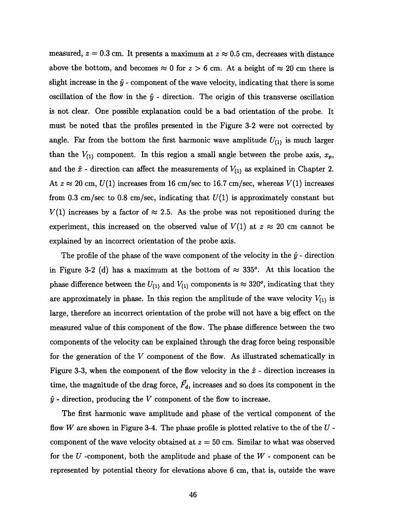
measured, z = 0.3 cm. It presents a maximum at z 0.5 cm, decreases with distance

above the bottom, and becomes ; 0 for z > 6 cm. At a height of ^ 20 cm there is

slight increase in the y - component of the wave velocity, indicating that there is some

oscillation of the flow in the Y - direction. The origin of this transverse oscillation

is not clear. One possible explanation could be a bad orientation of the probe. It

must be noted that the profiles presented in the Figure 3-2 were not corrected by

angle. Far from the bottom the first harmonic wave amplitude U(1) is much larger

than the V(1) component. In this region a small angle between the probe axis, xp,

and the X - direction can affect the measurements of V(1) as explained in Chapter 2.

At z 4 20 cm, U(1) increases from 16 cm/sec to 16.7 cm/sec, whereas V(1) increases

from 0.3 cm/sec to 0.8 cm/sec, indicating that U(1) is approximately constant but

V(1) increases by a factor of e 2.5. As the probe was not repositioned during the

experiment, this increased on the observed value of V(1) at z ~~ 20 cm cannot be

explained by an incorrect orientation of the probe axis.

The profile of the phase of the wave component of the velocity in the Y - direction

in Figure 3-2 (d) has a maximum at the bottom of r 3350. At this location the

phase difference between the U(1) and V(1) components is ; 3200, indicating that they

are approximately in phase. In this region the amplitude of the wave velocity V(1) is

large, therefore an incorrect orientation of the probe will not have a big effect on the

measured value of this component of the flow. The phase difference between the two

components of the velocity can be explained through the drag force being responsible

for the generation of the V component of the flow. As illustrated schematically in

Figure 3-3, when the component of the flow velocity in the 2 - direction increases in

time, the magnitude of the drag force, Fd, increases and so does its component in the

y - direction, producing the V component of the flow to increase.

The first harmonic wave amplitude and phase of the vertical component of the

flow W are shown in Figure 3-4. The phase profile is plotted relative to the of the U -

component of the wave velocity obtained at z = 50 cm. Similar to what was observed

for the U -component, both the amplitude and phase of the W - component can be

represented by potential theory for elevations above 6 cm, that is, outside the wave

i V

tA t 2 UT/2

Ub• i

V •, •. 43t

-' U xx

0/VFRipple axis Ripple axis

Figure 3-3: Schematic representation of the near-bottom flow in the pure wave ex-

periments, where Ub is the maximum near-bottom wave orbital velocity

boundary layer. The wave amplitude decreases with height and the phase remains

constant for z > 6 cm.

Using the measurements of the first harmonic amplitude and phase of the velocity

components in the (X, Y) direction, it is possible to construct the amplitude and the

phase profiles of the wave velocity components in the (, Xll) - directions by using

the transformation:

U_ = U cos9 - V sin9 (3.1)

U11 = U sin8 + V cos0

These profiles are presented in Figure 3-5. The amplitude and the phase of the wave

component in the direction perpendicular to the ripple axis in Figure 3-5 (a) and (c),

respectively, present similar characteristics to those observed in the U - component

of the velocity. For distances above a 4 to 6 cm the profiles can be described by the

potential theory solution. Inside the wave boundary layer the phase decreases with

height and the amplitude of the velocity presents the overshoot at z ; 2 cm, similar

to but stronger than the one observed in the U(1) component profile. In constrast, the

amplitude and phase of the component of the velocity in the direction parallel to the

ripple axis do not present any significant change in their profiles at z r 6 cm. The

Ub

I

1U

101Eo

100

I 1

1U

101

N 0100

IA'

0 2 4 6 -2 0 2 4W(1) (cm/sec) phase(W(1)) (radians)

Figure 3-4: First harmonic wave amplitude and phase of the component of the wavevelocity in the Z direction obtained for 0 = 450 in the experiments without the beads

wave amplitude remains approximately constant throughout the region between z

1.5 to 20 cm with only a very small overshoot in the wave amplitude at a heigh of

z 0 1.5 cm.

There is a remarkable difference in the profiles of the wave amplitude and phase

of the components of the flow in the direction perpendicular and parallel to the ripple

axis. In the direction perpendicular to the ripple axis, a large wave boundary layer

thickness indicates larger turbulence intensities, therefore larger bottom roughness.

On the other hand, the flow in the direction parallel to the ripple axis presents a

thinner wave boundary layer indicating that the bottom roughness experienced by

the flow in this direction is smaller than the one experienced by the component of the

flow in the direction perpendicular to the ripple axis.

3.1.2 Wave Energy Attenuation Experiments

The energy dissipation of the generated waves was measured when the ripples were

placed at 0 = 00, 300, 450 and 600 with respect to the direction of the incident wave.

a)

.8000 as00

b)

· 0 00.00of

4 ̂ 2 4 ̂ 2

5 10 15 20U(1)-perpendicular (cm/sec)

102

101

0 0.5 1 1.5 2phase(U(1)-perpendicular) radians

10

0 1I-0.2-0.2

U(1)-parallel (cml/sec)

0 0.2 0.4phase(U(1)-parallel) radians

Figure 3-5: First harmonic amplitude and phase for the case of 0 = 450 in theexperiments without beads. a) U(1)± the amplitude of the component of the velocityin the X^ - direction. b) U(1)11 the amplitude of the component of the velocity in the!I, - direction. c) phase of the velocity component in the ^i - direction. d) phase ofthe velocity component in the I11 - direction.

102

10

10l

-101IV 00

102

101

10"

10

d)

R.

* *

* S *Q'e *

:~JPe. 0

A

A A

1

The energy dissipation can be expressed in terms of an energy friction factor, fe. The

details of the procedure followed to obtain the energy friction factor can be found in

Mathisen and Madsen (1996). The free surface was measured at 33 locations along the

flume at 0.5 m intervals. The measured first harmonic wave amplitude is expressed

as:

;I¢ M ai(x) + a7 cos(2kx + P) (3.2)

where x is the position along the X - axis measured from the wavemaker, a2 and a,

are the amplitudes of the incident and the reflected waves, respectively, 0 is the phase

difference between the incident and reflected wave , and, k is the wave number. The

amplitude of the incident wave is assumed to decay linearly with respect to x:

ai = A + B x (3.3)

where A corresponds to the amplitude of the incident wave at the wavemaker and B is

the wave attenuation slope. To obtain the energy friction factor, f,, the representative

wave amplitude was assumed to be the amplitude of the incident wave a2 evaluated

at the mid-point between the first and the last location of measurement: xzo 10

m measured from the wave-maker. The results of the experiments are summarized

in Table 3.1. The values of the fe listed in the table were obtained after accounting

for sidewalls dissipation. The listed value ub 17 cm/sec corresponds to the near-

bottom orbital velocity predicted by potential theory based on a2(xo). The main

source of error involved in the estimation of fe, is given by the variability in the wave

attenuation slope: B. The attenuation experiments were repeated at least twice for

each angle and the error estimate based on the variability of the parameter B is

the one listed in the Table 3.1. The relative error of the fe estimates varies from

approximately 10% to 30% when the angle 0 increases from 00 to 600. From the

results shown in Table 3.1 , it is clear that the energy friction factor is a function of

the angle between the wave direction and the ripple axis. To uncover the dependency

of the energy friction factor on the angle of incidence a simple analysis is presented.

Assuming that the skin friction can be neglected, the energy dissipation inside the

TABLE A)NO BEADS

0 A (cm) B.10-4 ai (cm) a, (cm) P (rad) Ub (cm/sec) fe

0 5.14 -3.71 4.71 0.67 -5.77 17.05 0.25±0.0330 5.18 -3.29 4.80 0.79 -5.77 17.34 0.21±0.0345 5.16 -2.25 4.90 0.76 -5.67 17.64 0.13±0.0360 5.20 -1.50 5.03 0.84 -5.70 18.03 0.07±0.02

TABLE B)BEADS

0 A (cm) B.10 ai (cm) ar (cm) (rad) Ub (cm/sec) fe0 5.14 -2.90 4.81 0.71 -5.77 17.34 0.18±0.004

30 5.25 -2.55 4.95 0.82 -5.77 17.84 0.14±0.0145 5.18 -1.85 4.97 0.76 -5.67 17.85 0.09±0.0160 5.24 -1.45 5.07 0.84 -5.70 18.19 0.06±0.01

Table 3.1: Pure Wave attenuation experiments. A) Experiments without beads. B)Experiments with beads.

wave boundary layer is only due to drag. Following the approach of Kajiura (1968),

the energy dissipation Ed per unit area, averaged over a wave period is given by:

Ed = eT. .Ub (3.4)

where the overbar represents the time average, 7• is the bottom shear stress and

Ub = Ub cos wt is the velocity at the edge of the wave boundary layer z = w,.

The energy dissipation can be expressed in terms of the energy friction factor:

Ed = fe U• (3.5)4

As shown in Figure 3-2, the first harmonic amplitude of the wave velocity in the Y- direction has a maximum value at the bottom and decreases with height. At the

elevation of z = b the amplitude of the V(1) - component is negligible. Although

velocity measurements were not performed for other angles than 0 = 450, it is rea-

sonable to expect the effect of the bottom to be negligible at the edge of the wave

boundary layer. Therefore, the V - component of the flow can be neglected. Under

--

this assumption, the near-bottom orbital velocity can be considered to be in the I -

direction: Ub = Ub cos Wt 1 and the scalar product in Eq. (3.4) involves only the

- component of the bottom shear stress: r,,. The bottom resistance experienced by

the flow is represented by •' and can be expressed in terms of the drag force:

FdaT,, = Fd- (3.6)

where A is the distance between two ripple crests, (measured in the i± - direction),

and the subscript x indicates the projection of the drag force in the 2 - direction

given by: Fdx = Fd cos 0. The drag force is assumed to have the following time

dependency:

Fd = - Cd 9 Url JUJ il (3.7)2

where Cd is the drag coefficient, gr is the ripple height, which for the experiments

without beads is 77 = 1.5 cm and for the experiments with beads is q = 1.5 cm -

d = 0.9 cm, and UrI is the reference velocity that depends on time. The reference

velocity in Eq (3.7) is assumed to be given by the perpendicular component of the

flow velocity at the edge of the wave boundary layer:

Ur± = ub cosW t cos 0 (3.8)

Replacing Eqs. (3.8) to (3.5) into (3.4) the result obtained after taking the time

average is:f, U3 4 1 /4 3 Cd iU COS3 0 (3.9)4 3-7r 2 A

Eq. (3.9) suggests that fe is proportional to cos 3 0 if the value of the drag coefficient

Cd is independent of 0, and if the proper choice of the reference velocity is the velocity

component in the direction perpendicular to the ripple axis.

The values of f, in Table 3.1 were fitted by the least square method vs cos3 9

according to:

fe = m cos30 + b (3.10)

A) fe R m b Cd

No Beads 0.9823 0.21±0.03 0.05±0.02 1.65±0.22Beads 0.9945 0.14±0.01 0.05±0.01 1.77±0.13B) fed R m b Cd

No Beads 0.9826 0.22±0.03 0.04±0.02 1.72±0.23Beads 0.9940 0.16±0.01 0.02±0.01 2.09±0.16

Table 3.2: Fitting parameters according to Eq. (3.10). A) fe vs 0 B) fed vs 0 obtainedby the second approach described in text.

The resulting parameters obtained in the fitting, the correlation coefficient, R , the

slope, m, and the intercept, b, are presented in Table 3.2 (A). The drag coefficient

listed in the last column of the table was obtained from Eq (3.9) and (3.10) as a

function of the estimated slope, m, as:

37r ACd = m (3.11)

8 r7

The error of Cd listed in the last column of the table was estimated based on the

standard deviation of the slope m obtained by fitting Eq. (3.10) with the least square

method.

The analysis presented is based on the assumption that the energy dissipation

is due only to drag. This approximation is not necessarily true. In the case of the

experiments with beads the contribution of the energy dissipation due to skin friction

could be important. To take into account the skin friction term in the evaluation of

the total energy dissipation it is assumed, that

Ed = " b + - ' " U, (3.12)

The first term of the equation corresponds to the energy dissipation due to drag and

is expressed as a function of the drag force as done before to obtain Eq. (3.9). The

second term is the energy dissipation due to skin friction, where U is now the flow

velocity at z = 6', the thickness of the wave boundary layer due to skin friction. In

principle, 6•, is unknown, and is assumed to be proportional to J6 0 -i u,,/w, where

u', is the skin shear velocity defined based on the skin friction bottom shear stress

as: u', = r'1 /p. The factor multiplying the skin friction term, A'/A, takes into

account the fact that when there is a layer of beads between the ripples, the effective

distance over which the skin friction bottom shear stress acts is A' = A - 277. The skin

friction bottom shear stress can be expressed in terms of an energy friction factor due

to skin friction, f,, as:

" = f 3 b(3.13)

Using Eqs. (3.13) and (3.12), the total energy friction factor is written as:

f 3 A 13

fe U3 = fed U + fe' ub (3.14)

where, fed, the energy friction factor due to drag is introduced to represent the drag

term contribution to the total energy dissipation. From Eq. (3.14) the energy friction

factor due to drag is expressed as a function of the total energy friction factor obtained

in the wave attenuation experiments and the energy friction factor due to skin friction:

fed = fe - A' (-Ub3 (3.15)Ub

The problem now is to evaluate the skin friction factor, f', and u'. Two ways of

estimating f' are considered.

The first approach is to assume that the flow close to the bottom is described

by the model proposed by Grant and Madsen (1986). This model is applied in the

following way:

i) Using the measured values of fe and the near-bottom orbital velocity Ub as input

parameters to the model, the wave velocity, u,(z), inside the wave boundary layer is

obtained.

ii) Assuming a given value of J, smaller than J, an estimate of u' is obtained by

evaluating the velocity predicted in i) at z = 6•: u•' = uw,(').

iii) The model is applied again using as input the value of u' obtained in ii) and the

bottom roughness given by z" = d/30 under the assumption of rough turbulent flow.

In this way the shear velocity u', = fV , 2 I' is determined, and therefore a new

estimate of 6, = 2 , u,.,/w is obtained.

The process is repeated until the assumed value of 6" in i) agrees with the value

obtained in iii). Following this procedure, the value of the energy friction factor due

to skin friction obtained for the experiments with beads is listed on the third column

of Table 3.3 (B) under the heading f'(I).

The second approach to obtain f, is to assume that u' is given by the wave velocity

obtained in i) at the ripple crest: u' = uw(z = 77). Then, the Grant-Madsen model

is solved by specifying u, and the roughness z" = d/30. The resulting values of

f' obtained by using this approach are listed in the fourth column of Table 3.3 (B)

under the heading f'(II).

This method was also applied to the experiments without the beads. In this

case, the Grant-Madsen model is solved by specifying u' = uw(rq) and the bottom

roughness, which without beads is given by z, = v/(9 u',) assuming the flow is

smooth turbulent. The estimates of f' for the experiments without beads are listed

in the Table 3.3 (A).

Having the values of u' and f' Eq. (3.15) is used to evaluate the energy dissipation

due to drag. The corresponding results of fed for each of the experiments are listed

in the last column of Table 3.3.

The error in the estimates of fed is mainly related to the variability of the to-

tal energy friction factor, fe (listed in the second column of Table 3.3). The results

presented in Table 3.3 show that the two proposed methods of estimating fed give

virtually identical results result. Comparing the listed values of fe and fed, the con-

tribution of the skin friction to the total energy dissipation is negligible, except for

the case of the experiments with beads when 0 = 600.

The listed values of fed obtained by using the second approach were fitted vs

cos3 0. Using Eq. (3.11) the value of the drag coefficient was obtained and are shown

in the last column of Table 3.2 (B). For the case of the experiments without beads

Cd = 1.72 ± 0.23, and for the experiments with beads Cd = 2.09 ± 0.16. The error of

TABLE A)NO BEADS

9 fe f(II() fed(II)0 0.25±0.03 0.013 0.24± 0.03

30 0.21±0.03 0.013 0.20± 0.0245 0.13±0.03 0.011 0.12± 0.0360 0.07±0.02 0.011 0.06± 0.02

TABLE B)BEADS

0 fe fe(I) f'(II) fed(I) fed(II)0 0.18±0.004 0.044 0.055 0.17 +0.004 0.17 ±0.005

30 0.14±0.010 0.043 0.049 0.14 ± 0.01 0.13 ± 0.0145 0.09±0.010 0.043 0.045 0.09 ± 0.02 0.07 ± 0.0260 0.06±0.010 0.043 0.043 0.04 ± 0.01 0.03 ± 0.01

Table 3.3: Energy friction factor due to drag fed vs 9. A) Experiments with no beads:f, is obtained using the second method explained in the text. B) Experiments withbeads: f' is obtained by using the two methods explained in the text. (I) indicatesthe first method, and (II) the second method.

Cd was estimated based on the standard deviation of the slope m obtained by fitting

of Eq. (3.10) with the least square method.

The fitting parameters obtained are listed in Table 3.2 (B) and the resulting curve

is shown in the Figure 3-6. The intercept b corresponds to the limiting case of ripples

parallel to the direction of wave propagation (0 = 900), therefore, it is expected b = 0.

After accounting for skin friction, the values of b (Table 3.2 (B)) are slightly smaller

than the values of b obtained by fitting the total energy friction factor fe vs. cos3 8

(Table 3.2 (A)). The resulting slope obtained based on the fitting of fed is bigger than

the one obtained based on the fitting of fe. This result is reflected in the values of

Cd obtained by using Eq. (3.11). Although the values of the correlation coefficient

is not very heigh, the fitted line in Figure 3-6 lies inside the range of the estimated

error of the measurements.

It is concluded that the energy friction factor due to drag fed oc cos3 0. This result

was obtained by assuming that the drag force is scaled by the square of the reference

velocity in the perpendicular direction, UI.

0.0 0.2 0.4 0.q 0.8 1.0cos 0

0.0 0.2 0.4 0.4 0.8 1.0cos O

Figure 3-6: Fitting of fed vs cos3 . a) Experiments with no beads b) Experimentswith beads. The fitting parameters are listed in Table 3.2 B)

a)

0.40

0.30

• 0.20

0.10

0.00

0.20

0.15

- 0.10

0.05

b)

· ·

_ · · · · ·

_ __

n0 n I . I . I . I . I . I iL.

3.2 Pure Current Experiments

3.2.1 Description of the measurements

In this section the main characteristics of the flow observed in the measurements

performed when the current is incident at an angle with respect to the ripple axis are

described based on the experiments made for the case of 9 = 450 without beads. The

rest of the experiments performed are presented in Appendix A. All the pure current

profiles were corrected by angle using the criterion explained in Chapter 2.

In Figure 3-7 a vector plot of the (V, W) components of the flow measured for the

case when the ripples were placed at an angle 0 = 450 with respect to the incident

current is shown. The horizontal axis in the vector plot is the distance measured

along the Y - direction divided by the flume width: b = 76 cm. The vertical axis

is the distance above the bottom normalized by the water depth h = 60 cm. The

incident current is in the ^ - direction pointing out of the figure.

The figure shows that at the lower height measured: z = 3 cm above the bottom,

the V - component of the velocity is approximately uniform at the center region of

the flume with a magnitude of P 2.2 cm/sec. Close to the free surface, at z = 54 cm,

V = -1.5 cm/sec at the center region.

Because of the physical limitation of the traverse system it was not possible to

measure the flow very close to the walls of the flume. But there is evidence based on

flow visualization of suspended particles in the water that the flow close to the left

wall, y/b = 0, is directed downwards and the flow close to the right wall, y/b = 1, is

directed upwards implying that the flow can be approximately described as one cell

rotating anti-clockwise.

As mentioned in Chapter 2, the velocity profiles were obtained by moving the

traverse system along the ^ - axis at steps of P 1 cm between the two crests. The

vector plot of the (U, W) - components of the flow measured at the center of the

flume, y/b = 1/2, for 0 = 450 is presented in Figure 3-8 (a). Only the velocity vectors

close to the bottom, z < 4 cm, are shown. The horizontal axis is in the X - direction,

i.e., the direction of the incident current. The first profile was measured above the

0.8

0.6

0.4

0.2

S o0.1 0.2 0.3 0.4 0.5 0.6 0.7 0.8 0.9 1y/b

Figure 3-7: Vector plot of the (V, W) velocity components measured for 0 = 450 forthe NO BEADS experiments

crest located at x = 0 cm and the last profile was measured at x = 10/ cos 450

14.14 cm. The effect of the ripples on the flow is represented by the undulations seen

in the flow pattern. There is no evidence of flow separation at the ripple crest located

at x = 0 cm. The profile measured at x 12 cm was included in the vector plot for

completeness. It can be seen that the velocity at this location is approximately 0.

Analysis of the corresponding time series obtained showed that the signal acquired

with the ADV was influenced by reflections coming from the upstream side of the

ripple. Therefore, these points were not considered in the calculation of the spatial

average velocity profile. In Figure 3-8 (b) the velocity measurements close to the

bottom made when the flow was incident perpendicularly to the ripple axis, 0 = 00,

are shown in a vector plot of the (U, W)-components. The horizontal axis is in the ^

- direction, which is the direction of the incident flow. In contrast to Figure 3-8 (a),

the flow presents a well defined recirculation region downstream of the ripple located

at x = 0 cm. The flow separates at the crest and reattaches at a distance x k 5 cm.

The two experiments presented in Figure 3-8 (a) and (b) were performed using the

same flow conditions, i.e, a water depth of h = 60 cm and the same depth-averaged

1 cm/sec

-----i~ ~ i |i !J

4

3.5

3

2.5

2 51.5

1

0-5

-I8 10 12 14 16

x-perpendlcular (cm)

Figure 3-8: Detailed Velocity Field between two ripple crests in the NO BEADSExperiments: a) Vector plot of the (U, W) velocity components measured for 9 = 450,b) Vector plot of the (U, W) velocity components measured for 0 = 00, c) Vector plotof the (U±, W) velocity components measured for 9 = 450.

c2t m/sec a) 45

-* 4 -> -> -Z -4- -4-4- C-3 -3 ~

-. - - - -- 4 - -4 -- 3 -- C-- --. -~ -

"- -,~-

0 2 4 6x (cm)

3.

2.

1.

O

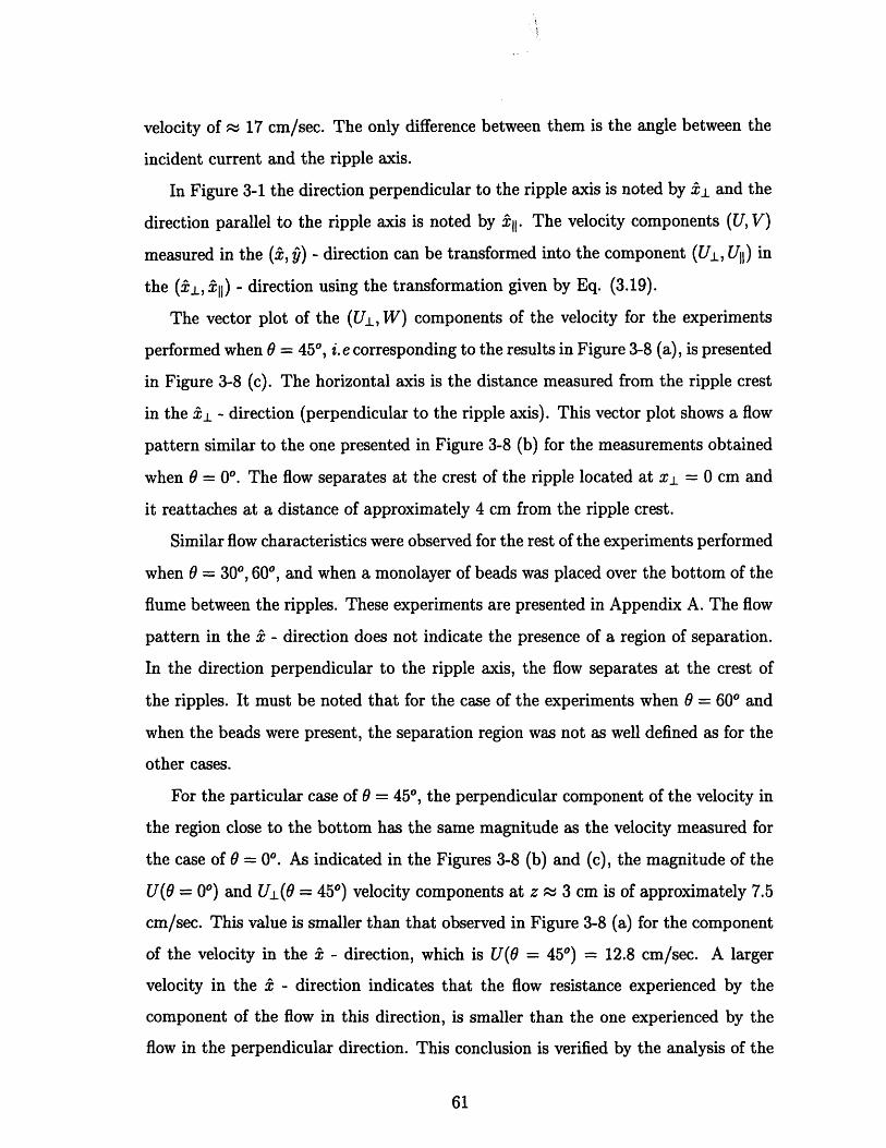
velocity of ;y 17 cm/sec. The only difference between them is the angle between the

incident current and the ripple axis.

In Figure 3-1 the direction perpendicular to the ripple axis is noted by ;i and the

direction parallel to the ripple axis is noted by 5X^. The velocity components (U, V)

measured in the (X;, ^) - direction can be transformed into the component (U±, U1) in

the (1±, 51) - direction using the transformation given by Eq. (3.19).

The vector plot of the (U±, W) components of the velocity for the experiments

performed when 0 = 450, i.e corresponding to the results in Figure 3-8 (a), is presented

in Figure 3-8 (c). The horizontal axis is the distance measured from the ripple crest

in the ;1_ - direction (perpendicular to the ripple axis). This vector plot shows a flow

pattern similar to the one presented in Figure 3-8 (b) for the measurements obtained

when 9 = 00. The flow separates at the crest of the ripple located at x1 = 0 cm and

it reattaches at a distance of approximately 4 cm from the ripple crest.

Similar flow characteristics were observed for the rest of the experiments performed

when 9 = 300, 600, and when a monolayer of beads was placed over the bottom of the

flume between the ripples. These experiments are presented in Appendix A. The flow

pattern in the & - direction does not indicate the presence of a region of separation.

In the direction perpendicular to the ripple axis, the flow separates at the crest of

the ripples. It must be noted that for the case of the experiments when 9 = 600 and

when the beads were present, the separation region was not as well defined as for the

other cases.

For the particular case of 9 = 450, the perpendicular component of the velocity in

the region close to the bottom has the same magnitude as the velocity measured for

the case of 9 = 00. As indicated in the Figures 3-8 (b) and (c), the magnitude of the

U(O = 00) and U(9O = 450) velocity components at z ; 3 cm is of approximately 7.5

cm/sec. This value is smaller than that observed in Figure 3-8 (a) for the component

of the velocity in the X^ - direction, which is U(O = 450) = 12.8 cm/sec. A larger

velocity in the X - direction indicates that the flow resistance experienced by the

component of the flow in this direction, is smaller than the one experienced by the

flow in the perpendicular direction. This conclusion is verified by the analysis of the

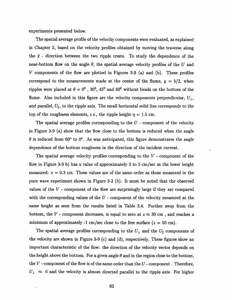
experiments presented below.

The spatial average profile of the velocity components were evaluated, as explained

in Chapter 2, based on the velocity profiles obtained by moving the traverse along

the X - direction between the two ripple crests. To study the dependence of the

near-bottom flow on the angle 0, the spatial average velocity profiles of the U and

V components of the flow are plotted in Figures 3-9 (a) and (b). These profiles

correspond to the measurements made at the center of the flume, y = b/2, when

ripples were placed at 0 = 00 , 300, 450 and 600 without beads on the bottom of the

flume. Also included in this figure are the velocity components perpendicular, U±,

and parallel, U1 , to the ripple axis. The small horizontal solid line corresponds to the

top of the roughness elements, i.e., the ripple height 77 = 1.5 cm.

The spatial average profiles corresponding to the U - component of the velocity

in Figure 3-9 (a) show that the flow close to the bottom is reduced when the angle

0 is reduced from 600 to 00. As was anticipated, this figure demonstrates the angle

dependence of the bottom roughness in the direction of the incident current.

The spatial average velocity profiles corresponding to the V - component of the

flow in Figure 3-9 b) has a value of approximately 3 to 5 cm/sec at the lower height

measured: z = 0.3 cm. These values are of the same order as those measured in the

pure wave experiment shown in Figure 3-2 (b). It must be noted that the observed

values of the V - component of the flow are surprisingly large if they are compared

with the corresponding values of the U - component of the velocity measured at the

same height as seen from the results listed in Table 3.4. Further away from the

bottom, the V - component decreases, is equal to zero at z ; 30 cm , and reaches a

minimum of approximately -1 cm/sec close to the free surface (z = 50 cm).

The spatial average profiles corresponding to the U1 and the UII components of

the velocity are shown in Figure 3-9 (c) and (d), respectively. These figures show an

important characteristic of the flow: the direction of the velocity vector depends on

the height above the bottom. For a given angle 9 and in the region close to the bottom,

the V - component of the flow is of the same order than the U - component . Therefore,

UL M 0 and the velocity is almost directed parallel to the ripple axis. For higher

5 10U (cm/sec)

102

101

15 20

10

i -1IV

-2 0 2V (cm/sec)

102

101

10,

10-1

0 5 10 15U-perpendicular (cm/sec)

4 6

10U-parallel (cm/sec)

Figure 3-9: Spatial average velocity profiles of the NO BEADS experiments at thecenter of the flume, y/b = 1/2, as a function of the angle 0. a) U, b) V, c) U± and d)UII - component. The symbols correspond to the different ripple configurations used:... 0 = 0o, * = 300, o = 450, + 9 = 600. The top of the roughness element isindicated by the horizontal solid line

0

101

10'

100

I fl 1I 0

0

102

10o

10-110

·

I

AI1

I

1%*

I.%

NO BEADS

BEADS

300450600

300450600

U (cm/sec) V (cm/sec)2.79 4.186.24 5.297.70 3.43

U (cm/sec) V (cm/sec)

3.34 2.785.47 3.365.83 2.10

Table 3.4: Velocity components in the (^, Y) direction measured at z = 0.3 cm abovethe bottom at y/b = 1/2 in the pure current measurements

elevations, the UL - component becomes more important, and the velocity vector will

start to rotate from being directed parallel to the ripple axis to being directed parallel

to the incident flow at elevations where the V - component is negligible. It is observed

in the figure, that the magnitude of the parallel and perpendicular components of the

flow depends on the angle 0. By definition, U± cx U cos 0 and U1l oc U sin 9. The

resulting effect is a decrease of UL and an increase of U11 when the angle 0 increases.

In order to study the spatial dependence of the experimental results due to the

finite width of the flume, the velocity measurements performed at the center of the

flume, y/b = 1/2 were repeated at two other locations along the ^ - axis: y/b = 3/8

and y/b = 5/8.

In Figure 3-10 the spatial average profiles of the U, V, UI and U11 components of

the velocity are presented for the case of 0 = 450. The different symbols correspond to

the profiles measured at three different locations along the Y - axis: y = 3b/8, y = b/2

and y = 5b/8. The profiles share the same characteristic: close to the bottom, for

elevations below 4 cm, the velocity is virtually independent of the y - location. The

spatial average velocity profile of U and U± obtained in the experiments without

beads at y = b/2 and 0 = 450 are represented by the circles in Figure 3-11 (a) and

(b), respectively. The figure show a well defined logarithmic region between z = 1.5

cm and z = 6 to 7 cm. The dotted line represents the logarithmic fitting obtained as

explained in the next section.

"

5 10U (cm/sec)

1u

101

100

-1

15 20 -2 0 2V (cm/sec)

102

101

10,

-110

5 10 15U-perpendicular (cm/sec)

10U-parallel (cm/sec)

Figure 3-10: Spatial average velocity profiles of experiments as a function of y mea-sured for 9 = 450 and NO BEADS. a) U, b) V, c) U1 and d) U1l - component. Thesymbols correspond to + y/b = 3/8, o y/b = 1/2 and * y/b = 5/8. The top of theroughness element is indicated by the horizontal solid line.

10

101

10

0

102

101

4 6

d)

loi

6 - 1

IV

0

------------ mr-

---

.12

AA

A A

For higher elevations the velocity profiles present a change in slope and at z =

30 cm they exhibit a maximum and then they start to decrease. In the upper region

of the flume the velocity depends on the y - location. Close to the right wall of the

flume, y = 5b/8, the U-component of the velocity is smaller than the corresponding

profile close to the left wall, y = 3b/8.

Since, the lower region of the flow is the one considered for the purpose of studying

the mechanism of the generation of the lateral flow and for predicting the bottom

resistance experienced by the flow, the behavior of the flow in the upper part of the

water column is of minor importance.

3.2.2 Analysis of the Pure Current Velocity Profiles

Close to the bottom the spatial average velocity profiles present a well defined loga-

rithmic region between 1.5 cm up to approximately 7 cm. Values of the shear velocity

and bottom roughness obtained by fitting a logarithmic velocity profile in the region

close to the bottom are listed in Table 3.5 (A) for the experiments without beads, and,

in Table 3.5 (B) for the experiments with beads. The subscripts x and I correspond

to the ^ and I1 directions, respectively. The number of points used in the fitting was

between 5 to 7. The theoretical level used for the experiments with no beads was the

bottom of the flume and for the experiments with beads it was 0.35d below the top of

the beads (Mathisen 1993, Jackson 1981), where d = 0.64 cm is the bead diameter.

The error of the shear velocity were estimated based on a 95% confidence level.

Depending on the number of points used for the fitting and the value obtained for

the correlation coefficient, R in Table 3.5, the resulting errors were of the order of

10% for u, and for u,±. The corresponding errors obtained for the bottom roughness

were of the order of 30% for zox and 20% for z, 1 . The values of the shear velocity and

bottom roughness obtained from the fitting of the parallel component of the velocity

are not included in Table 3.5. The resulting correlation coefficients obtained for this

component of the velocity were in general low and the error estimated for zol 0.8zoll11.

When the angle is changed from 0 = 00 to 0 = 600 the value of the roughness

corresponding to the x-component of the velocity, zox, varies from 0.36 cm to 0.01 cm

70'

'V

700

OO

~o0

0

0. .o o.9 ..

...o...o

-o-

.. ..

o go

00 0

0 00 0

o00

....

...

... .

.o

-

.o o

-.o

.o

o.....

.70

Table A)NO BEADS

o0

0

303030

454545

606060

Table B)BEADS

0o

0

303030

454545

606060

y/b R U*xu, Zo R1 u, 1 zo1 Ud U', Cd1/2 0.9965 1.37 0.36 0.9965 1.37 0.36 1.33 0.35 0.76

3/8 0.9978 2.04 0.29 0.9991 2.07 0.48 2.02 0.58 1.121/2 0.9984 1.59 0.16 0.9989 1.70 0.34 1.63 0.57 0.715/8 0.9986 1.59 0.17 0.9993 1.63 0.34 1.56 0.57 0.68

3/8 0.9995 1.59 0.12 0.9994 1.62 0.45 1.56 0.64 1.001/2 0.9992 1.31 0.06 0.9998 1.35 0.32 1.26 0.65 0.635/8 0.9990 1.21 0.05 0.9992 1.22 0.27 1.13 0.66 0.52

3/8 0.9991 1.05 0.02 0.9999 1.09 0.43 1.02 0.69 0.901/2 0.9972 1.01 0.02 0.9967 0.96 0.37 0.88 0.67 0.765/8 0.9888 0.92 0.01 0.9967 0.84 0.28 0.74 0.69 0.48

y/bJ Rx U*x Zox RI u,1 Zol U*d U, Cd1/2 0.9977 1.11 0.17 0.9977 1.11 0.17 1.01 0.57 0.64

3/8 0.9974 1.48 0.12 0.9987 1.52 0.22 1.38 0.86 0.881/2 0.9987 1.42 0.12 0.9990 1.38 0.20 1.23 0.84 0.765/8 0.9943 1.28 0.10 0.9958 1.23 0.17 1.08 0.80 0.62

3/8 0.9995 1.31 0.08 0.9991 1.22 0.25 1.08 0.94 0.881/2 0.9981 1.19 0.06 0.9995 1.01 0.15 0.82 0.93 0.495/8 0.9998 1.16 0.05 0.9949 0.98 0.15 0.79 0.93 0.45

3/8 0.9959 1.08 0.03 0.9985 0.87 0.24 0.71 1.01 0.761/2 0.9980 1.03 0.03 0.9988 0.76 0.19 0.57 0.99 0.535/8 0.9985 0.90 0.02 0.9983 0.65 0.13 0.40 0.99 0.23

Table 3.5: Shear Velocities, Hydraulic Roughness and Drag Coefficients for the PureCurrent Experiments: A) Experiments without beads B) Experiments with beads.The correlation coefficient, shear velocity in (cm/sec) and bottom roughness in (cm)obtained by fitting a logarithmic velocity profile to the spatial average velocity mea-sured in the 2 - direction (indicated by the subscript x), and in the j± - direction(indicated by the subscript I. The shear velocities u' (cm/sec) and U,d (cm/sec) areobtained obtained according to Eqs. (3.19) and (3.24) respectively

for the experiments with no beads, and from 0.17 cm to 0.02 cm for the experiments

with beads. In contrast, the values obtained for the roughness corresponding to the

component of the velocity perpendicular to the ripple axis do not present a depen-

dency on the angle. For the experiments with no beads, the resulting value of the

perpendicular roughness obtained as the mean value of all the experiments is zo1 =

(0.36 ± 0.07) cm and for the experiments with beads, zo1 = (0.19 ± 0.04) cm. The

standard deviation represents a relative error of about 20% which is of the order of

the accuracy estimated from the fittings. The smaller value of zo1 obtained in the

experiments with beads can be explained by the fact that the effective ripple height

in these experiments is smaller than the ripple height in the experiments without the

beads. In the experiments without beads 7t = 1.5 cm and the ratio zo,±/i, 0.24. In

the experiments with beads the effective ripple height is q = 1.5 cm - d = 0.9 cm and

the ratio zo±/ 77 0.21.

From the analysis of the spatial average velocity profiles presented above it is

concluded that the bottom roughness experienced by the incident flow, z,, depends on

the angle 0. The roughness in the perpendicular direction: zox can be considered to be

independent of the angle and related to the ripple height with an approximate value of

zol 0.23rl, yielding an equivalent Nikuradse bottom roughness of kb = 30 Zo1 ; 777.

3.2.3 Determination of Cd.

The conclusion obtained from the analysis of the energy friction factor measured in

the wave attenuation experiments was that the appropriate reference velocity to be

used in the scaling of the drag force is the component of the velocity in the direction

perpendicular to the ripple axis. This result is used in this section to estimate the

drag coefficient from the measurements of the pure current velocity profiles.

The bottom resistance experienced by the flow consists of two contributions, the

skin friction and the form drag caused by the ripples, (Smith and McLean, 1977).

The bottom resistance related to the flow over two-dimensional roughness elements

of height q and spacing A is expressed in terms of a drag force Fd that is assumed to

4

Incident Flov

Figure 3-12: Schematic definition of the direction of the reference velocity i(zr = q).

be given by:

Fd = C d r7 U j1 (3.16)2

where p is the fluid density and Cd is the drag coefficient. The reference velocity, Ur,

is assumed to be the flow velocity in the direction perpendicular to the ripple axis at

the reference elevation zr = 77.

In this analysis the skin friction contribution is assumed to be the bed shear stress

produced when the ripples are not present and is expressed in terms of a shear velocity

U.:

7' = pu,2 & (3.17)

where & defines the direction of the flow velocity at the reference elevation zr = 77,

which is at an angle a with respect to the X^ - axis, as shown in Figure 3-12. The

total flow resistance per unit length in the x± - direction is expressed as:

ATbL = Fd + A'Tr (3.18)

where Tbi is the total bottom shear stress in the perpendicular direction and A' is the

effective distance over which the skin friction acts. For the experiments with beads

A' = A - 2 77, and for the experiments without beads A' = A. Expressing the total

bottom shear stress in the perpendicular direction in terms of a shear velocity u,±,

and introducing Eqs. (3.16) and(3.17) into (3.18) :

Au* 1 = C d vU + uA' "COs(O + o) (3.19)

If the skin friction is assumed to be negligible with respect to the drag contribution,

Eq. (3.19) becomes:

A uI = 1Cd 7 UV1 (3.20)

Expressing the reference velocity in the perpendicular direction as:

U1 = uJ ln( 1_) (3.21)

an expression for the drag coefficient is obtained using Eq. (3.21) in Eq. (3.20):

Cd = - (3.22)7 [ln(/zo1)]> 2

indicating that Cd depends on the ripple geometry, (A, r7) and on the roughness in the

perpendicular direction (zo±). The results obtained from the analysis of the spatial

average velocity profiles in the perpendicular direction presented in Table 3.5 show

that the bottom roughness zo01 was independent of the angle. Therefore, a constant

bottom roughness in the perpendicular direction is consistent with the assumption of

a constant drag coefficient.

If the skin friction term is not negligible, Eq. (3.19) must be used to obtain the

drag coefficient. In order to estimate the skin friction term it is assumed that the

flow velocity at the reference elevation is known and that the flow is described by the

law of the wall in the region between zo, the bottom roughness due to skin friction,

and zr = :

U(z,) = In(-) & (3.23)

The value of the bottom roughness due to skin friction is assumed to be given

by z' = v/9u' when the flow is smooth turbulent as expected for the experiments

without beads. For the experiments with beads the flow is assumed to be rough

turbulent, therefore, zo = d/30.

Knowing the magnitude and direction of the flow velocity at r7 measured in the

experiments, the value of u' can be obtained from Eq (3.23). With u,± estimated

from the fittings the resulting values of Cd from Eq. (3.19) are listed in the last

column of Table 3.5. For the experiments without beads Cd = (0.8 ± 0.2) and for the

experiments with beads Cd = (0.6 ± 0.2). Within the uncertainty of the estimates

the drag coefficient obtained in the experiments without beads is the same as the one

obtained in the experiments with beads.

Having determined the value of Cd the drag term in Eq. (3.19) can be evaluated

to obtain the shear velocity associated with the drag contribution to the total bottom

shear stress as:2 1 CCd U

ud- = U2 (3.24)

The values of the shear velocity corresponding to the skin friction shear velocity,

u', and the shear velocity associated with the drag contribution, Ud are also listed

in Table 3.5

The results show that the skin friction contribution becomes more important with

respect to the drag contribution when 0 increases from 00 to 600. After evaluating

the drag term it is obtained for the experiments with no beads that u 2 u,2 for 9

= 00 and uadd ,. 0.8 u,± for 9 = 600. For the experiments with beads ud P 0.8 u,1

for 9 = 00 and Usd , 0.4 u,1 for 0 = 600.

The analysis of the experimental velocity profiles presented in this section indicates

that the flow resistance experienced by a flow incident at an angle with respect to the

ripple axis can be expressed in terms of a drag force. The drag coefficient obtained is

independent of the angle of incidence and the drag force is scaled by the square of the

reference velocity in the direction perpendicular to the ripple axis at the elevation of

the ripple crest.

Chapter 4

Pure Current Model for

Experimental Conditions

In Chapter 3 the experiments performed when the current is incident at an angle

with respect to the ripple axis were described. The measurements showed that near

the bottom the V - component of the velocity is of the same order than the U -

component. In this chapter the concept of a drag force oriented perpendicular to the

ripple axis is introduced in a simple model to described the observed near-bottom

flow.

In Figure 4-1 the incident flow, uo, is assumed to be in the X - direction. The

angle between the ripple axis and the ^ - direction is 0. The bottom shear stress

in the direction perpendicular to the ripple axis is balanced by the drag force. The

component of the shear stress in the parallel direction to the ripple axis is initially

unbalanced and is used to represent a driving force that will induce the fluid to move

along the ripple axis.

Because the flume has a finite width the lateral flow does not have time to become

fully developed. Therefore, the velocity consists on two components. One component

is represented by the steady state, uo, in the X - direction. The other component is

the time-dependent velocity in the direction parallel to the ripple axis caused by the

unbalanced component of the shear stress.

u0

Dragforce

x,,

0) Driving force

r-..-- - - - - -

Figure 4-1: Definition of the Reference System The incident flow, uo is in the i -direction. The perpendicular component of the bottom shear stress, -Tob is balancedwith the Drag force. The Driving force is in the direction parallel to the ripple axis,

4.1 Description of the model

The flow is assumed to be driven by a uniform pressure gradient. The pressure

gradient is in the i - direction and is defined in terms of a shear velocity u,:

dpo U2= p - (4.1)ax h

where h is the water depth.

The flow is assumed to be uniform:

+ = 0 (4.2)ax Oz

where To is the shear stress and is assumed to be:

auoTo = P vot aZ (4.3)

zand,, z(1 -zh) is the eddy viscosity. The flow is initially represented by

and, vot = 's u. z(1 - z/h) is the eddy viscosity. The flow is initially represented by

p,

-_ Z__ 4

p IXII

U0 'l

u olxj_

t<O

Figure 4-2: Sketch of initial conditions for model developement. For times t < 0 theflow is in equilibrium and is given by u,. The component of the flow in the directionperpendicular to the ripple axis is: uo, and in the direction parallel to the rippleaxis is ull-

the usual logarithmic velocity profile:

u, zUo = - In() (4.4)

K Zo

The shear stress at the bottom can be decomposed in a component perpendicular

to the ripple axis, Tobi, and in a component parallel to the ripple axis, Tobll. The

perpendicular component is assumed to be balanced by the drag force. The parallel

component is, in principle, unbalanced and is assumed to represent a driving force in

the direction parallel to the ripple axis.

The time at which the driving force starts to act is defined as t = 0. For times

t < 0 , the flow is in equilibrium and can be written in the (±, I11) axis, Figure 4-2:

Uo = uo0l I + U01ll ll (4.5)

Combining Eqs (4.4) and (4.5):

Uo = - cos 0 In(-) (4.6)re zo

71

wmx

----- I

UO

t=tb/2

x

=0

Figure 4-3: Sketch of transformation from time to space At time t = tb/2 a fluidparticle initially located at xll = 0 reaches the center of the flume. The componentof the velocity in the parallel direction to the ripple axis is U11 = 01oll + ull(t = tb/2)

oll -sin In(zz) (4.7)n Xzo

Let us consider a fluid particle placed at the side wall of the flume, xll = 0. At t = 0

the driving force starts to act over the fluid particle, which is accelerated away from

the wall in the direction parallel to the ripple axis. After a given time, t = tb/2, the

fluid particle originally located at zxl = 0 will be in the center of the flume. The

velocity of the fluid particle at this location is is given by:

U(tb/2) = ol4.8)

Ull(tbl2) = Uoll + Ull(tb/2) (4.9)

where uoll is the time-independent part of U11 given in Eq. (4.7), and U1 1(tb/2) is

the time-dependent part of the velocity component in the parallel direction at t =

tb/2. As the forcing is assumed to be in the direction parallel to the ripple axis, the

perpendicular component of the velocity in Eq. (4.8) remains constant in time and

equal to uo0 given by Eq. (4.6).

In this analysis the velocity of the flow at the center of the flume in Eqs. (4.8)

a

and (4.9) is expressed as a function of the time t = tb/2. This time is defined as the

time needed for the fluid particle that is initially located at xll = 0 to reach the center

of the flume. The distance traveled by the particle between the side wall, xll = 0,

and the center of the flume along the direction parallel to the ripple axis is shown in

Figure 4-3, and is related to the time tb/2 by:

2 cos = b ull(z rl, t) dt (4.10)

where ull(z = rl, t) is the time dependent component of the velocity evaluated at the

top of the ripple z = r7.

The parallel component of the bottom shear stress given by:

Tobll = P u2 sin0 (4.11)

is used to represent the driving force. This driving force is expressed as an effective

pressure gradient acting over the fluid particles in the direction parallel to the ripple

axis:OPdriving U2

p = sin 0 f(z) (4.12)axii h

where f(z) is the spatial distribution of the driving force which is assumed to be:

h for z', < <

f(z) = " (4.13)0 for rl<z<h

where z, is the bottom roughness in the parallel direction and is given by the corre-

sponding bottom roughness due to skin friction.

The driving force starts to act by accelerating the near-bottom flow. At the same

time, the shear stress starts to increase and to compensate the effect of the driving

force by diffusion of vorticity. The equation describing the time dependent parallel

component of the velocity is written as:

U -L* sin0 f(z) + (4.14)at h 1z

where •i1 is the shear stress representing the diffusion term and is expressed in terms

of an eddy viscosity vt:

Bull(t)S1(z,,t) = p t uz (4.15)

In Eq (4.14) the convective terms have been neglecting by assuming that the flume

is wide compare to the water depth. To take into account the presence of the walls,

the origin of time has been defined as t = 0, when the flow is at the side- wall:

xll = 0 in Figure 4-3. For time t < 0 the flow is given by the steady solution u,. By

assuming that the perpendicular component of the velocity u_ is independent of time,

is equivalent to assuming that it does not depend on the y. This assumption can be

considered correct in the region of the flow defined by: z < 7 cm and 3b/8 < y < 5b/8

as is observed in the experiments shown in Figure 3-10 (c).

When time increases the gradient of the time-dependent component of the velocity

increases, therefore the shear stress in Eq. (4.15) changes with time. To solve for

ull(t) it is necessary to specify the eddy viscosity vt. For this purpose it is assumed

that the shear stress, 711, at the bottom is given by:

Tbl (t) = Trj(z',t) = a(t) TobIl (4.16)

where a(t) is in principle unknown and is obtained as part of the solution. Using Eq.

(4.11) in Eq. (4.16) we obtain:

rb11(t) = p u = p (t) u~ sine (4.17)

where u. 1ll is the shear velocity representing rbll, and can be written as:

U = 1u= (t) v/sinu(4.18)

In the region z,, < z < 7 the eddy viscosity, vt, is assumed to be scaled by the

shear velocity u,11, and in the region l < z < h, vt is assumed to be scaled by the

shear velocity that represents the driving pressure gradient of the initial flow, u,, in

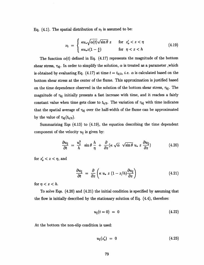
Eq. (4.1). The spatial distribution of vt is assumed to be:

Vt { su.in z for z," < z < 7 (4.19)Icu.z(1 - ) for r7< z < h

The function a(t) defined in Eq. (4.17) represents the magnitude of the bottom

shear stress, Tbll. In order to simplify the solution, a is treated as a parameter ,which

is obtained by evaluating Eq. (4.17) at time t = tb/2, i.e. a is calculated based on the

bottom shear stress at the center of the flume. This approximation is justified based

on the time dependence observed in the solution of the bottom shear stress, 'bll. The

magnitude of 'b11 initially presents a fast increase with time, and it reaches a fairly

constant value when time gets close to tb/2. The variation of rbll with time indicates

that the spatial average of rb1l over the half-width of the flume can be approximated

by the value of TbI (tb/2).

Summarizing Eqs (4.13) to (4.19), the equation describing the time dependent

component of the velocity ull is given by:

U 2 h 4 9ullull u, sin0 h + (± . sn u, z u Z ) (4.20)at h 77 z az

for zx < z < 7r, and

-i-= z u z (1 - z dh) (4.21)

for r7 < z < h.

To solve Eqs. (4.20) and (4.21) the initial condition is specified by assuming that

the flow is initially described by the stationary solution of Eq. (4.4), therefore:

ull(t = 0) = 0 (4.22)

At the bottom the non-slip condition is used:

u11(zo) = 0 (4.23)

At the free surface the shear stress is assumed to be equal to zero:

9 = 0 (4.24)

Continuity of the velocity and shear stresses is required at z = r7:

u11(7-) = ull(71 ) (4.25)

vt [u = t(4.26)

The solution of Eqs (4.20) to (4.26) was obtained at the time t = tb/2 defined in Eq.

(4.10).

Equations (4.20) to (4.26) were solved numerically by using a finite difference

method. The equations were time stepped with a standard explicit Euler scheme.

The details of the numerical solution are presented in Appendix B.

The equations involve the parameter a defined in Eq. (4.16), which is unknown.

The problem was solved by iteration on a. Assuming an initial value of a = 1, Eqs

(4.20) to (4.26) were solved to obtain ull(t = tb/2) and Tbll(t = tb/2). Using

Eq. (4.16) a new value of the parameter a(t = tb/2) was obtained. This new value

of a was used to solve again Eqs (4.20) to (4.26) . In this way a second estimate of

Tbl (t = tb/2) and a was calculated. This process was repeated until convergence of a

was achieved within three significant digits.

4.2 Model Solution and Comparison with the Ex-

periments

To obtain the time-dependent component of the flow by using Eqs. (4.20) to (4.26)it

is necessary to specify the driving force, that is u, and the bottom roughness z", must

be known. For the experiments with beads z, = d/30 and for the experiments without

beads, z" = v/(9u. y/avf•is ), corresponding to smooth turbulent flow.

The perpendicular component of the velocity can be written as:

u±-- In( -) (4.27)/ Zo I

Comparing Eq. (4.27) and (4.6), the value of u, can be obtained as a function of the

shear velocity of the perpendicular component of the flow:

u_. = (4.28)cos 0

zo = Zo1 (4.29)

Having the value of u, the driving force in Eq. (4.13) is known and the ull can be

obtained by solving Eqs. (4.20) to (4.26) iterating on a as explained in the previous

section.

After solving for the ull at time t = tb/2, the component of the velocity in the i

and 9 - directions were obtained:

U(tb/2) = U(tb/2) sin0 + u1 cos0 (4.30)

V(tb/2) = Ul(tb/2) cosO - u1 sin0 (4.31)

where Ull(tb/2) = Uol] + Ull(tb/2) and uo11 and u1 are given by Eqs. (4.6) to (4.7). The

values used of us, and zox were those obtained by fitting a logarithmic profile to the

measured perpendicular component of the velocity. These parameters were presented

in Tables 3.5 (A) and (B) and are are summarized in Table 4.1. The calculated

velocity profiles obtained by using Eqs. (4.30) and (4.31) are compared with the

experiments in Figures 4-4 to 4-6 for the cases with beads, and in Figures 4-7 to

4-9 for the cases without beads. The solid line corresponds to the predicted velocity,

and the circles to the spatial average velocity profiles measured in the experiments.

For the case of the experiments with beads the theoretical bed was chosen at 0.35

times the bead diameter below the top of the beads. For each angle of incidence part

(a) of the figure corresponds to the perpendicular component of the velocity. As the

input parameters uj, and zo, were those obtained by fitting a logarithmic profile to

Table 4.1: Input parameters to the model: u,± and zo obtained by fitting a loga-rithmic velocity profile to the perpendicular component of the velocity (Tables 3.5)(A) and (B). A)Experiments with beads. B)Experiments without beads. The mea-surements were performed at y = b/2 for 0 = 300, 450 and 600.

the perpendicular component of the velocity, the theoretical and experimental points

must be the same by definition. Parts (b), (c) and (d) of the figures correspond to

the Ull, U and V components of the velocity, respectively.

The results presented in the figures show that the model is able to describe the

measured velocity. Although the predicted velocity overestimates the measurements

the behavior of the theoretical profiles is in agreement with the experiments. The

difference in the prediction and the measurements is more marked in the experiments

without the beads. For this case the model was solved assuming that the flow was

smooth turbulent.

The effect of the bottom roughness zo on the predicted profile in the experiments

without the beads was studied. The triangular bars simulating the roughness elements

were attached to the bottom of the flume by duct tape. Between two bars part of

the duct tape was covering the glass bottom of the flume. As the duct tape presents

a corrugation of approximately 1 mm, the model was applied to the experiments

without beads by assuming that flow was rough turbulent and the bottom roughness

was given by zo = 1 mm/30 r 0.003 cm. The resulting velocity profiles do not

present any improvement with respect to those obtained under the assumption of

smooth turbulent flow. The reason for this is that the resulting bottom roughness

obtained by assuming smooth turbulent flow: z" = v/(9u, ý/i/s-iO) 0.001 cm,

A) Beads 0 U*, (cm/sec) U* (cm/aec) zo± (cm) tb/2 (sec) a30 1.38 1.59 0.20 21.84 0.3845 1.01 1.43 0.15 22.35 0.4160 0.76 1.52 0.19 23.55 0.44

B) No Beads 09 Ug (cm/.ec) u, (cm/sec) Zo1 (cm) tb/2 (sec) a30 1.70 1.96 0.34 18.49 0.2145 1.35 1.91 0.32 17.21 0.2260 0.96 1.92 0.37 18.63 0.23

0 5 10 15Uperpendicular (cm/sec) Uparallel (cm/sec)

0 5 10 15 20 -2 0 2 4 6U (cm/sec) V (cm/sec)

Figure 4-4: Pure current velocity profiles measured at the center of the flume, y = b/2,for the experiments with beads and 9 = 300 a) U1 b) U11 c) U and d) V.

10'

10,

10710'

A

.v

.4n2

,0 ft

5 10 15Uperpendicular (cm/sec)

5 10U (cm/sec)

102

101

100

1 -1

15 20 I-2-2

Uparallel (cm/sec)

0 2V (cm/sec)


10

10

10,

IIV 0

10

10'

lou

I 1

IU

0 4 6

Pll

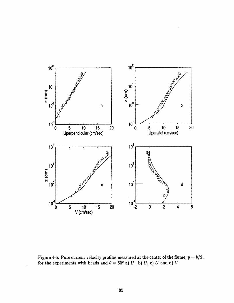
Uperpendicular (cm/sec)

0 5 10V (cm/sec)

102

101

100

-101n15 20 -2 0 2 4 6


102

10

10

i nl

a2

Uparallel (cm/sec)

A

SII f

102

101

100

4 1II I

Uperpendicular (cm/sec)

0 5 10 15 20U (cm/sec)

0 5 10 15 20Uparallel (cm/sec)

-2 0 2 4 6V (cm/sec)

Figure 4-7: Pure current velocity profiles measured at the center of the flume, y = b/2,for the experiments without beads and 0 = 300 a) U1 b) U11 c) U and d) V.

1'

1

1

102

100

,,2

.w

A

=

102

10

100

1 n"

5 10 15Uperpendicular (cm/sec)

5 10U (cm/sec)

0 5 10 15Uparallel (cm/sec)

102

101

10"i

15 20I-2

-2 0 2V (cm/sec)

Figure 4-8: Pure current velocity profiles measured at the center of the flume, y = b/2,for the experiments without beads and 0 = 450 a) Uj_ b) UII c) U and d) V.

102

101

100

0-1

00

102

101

1• 1

0I 4 6

102

10'

100

in-1

Uperpendicular (cml/sec)

0 5 10 15 20U (cm/sec)

I0

102

In1II-2-2

5 10 15Uparallel (cm/sec)

0 2V (cm/sec)

4 6

Figure 4-9: Pure current velocity profiles measured at the center of the flume, y = b/2,for the experiments without beads and 0 = 600 a) U1 b) UII c) U and d) V.

ý I

4 n2

Sn2

which is of the order of 1 mm/30.

The spatial distribution of the driving force defined in Eq. (4.13), implies that

the forcing is concentrated in the region z,, < z < r7. As a consequence of this

assumption,, the predicted V - component approaches zero a distance far from the

bottom, implying that there is a net flow in in the Y - direction. The lateral boundaries

of the flume imposed the constrain that the depth-average of the V - component of

the velocity must be equal to zero. This effect could be considered by introducing

a uniform pressure gradient in the (-Y) - direction that drives a "return" flow: v,.

An estimate of the return flow was obtained using the predicted V component of the

flow:

y= fVdz (4.32)h

The value obtained in this manner was vr 0.3 cm/sec. This value is small compared

with the predicted V component close to the bottom. Therefore, it is expected

that the predicted velocity profiles obtained after the incorporation of this pressure

gradient will not be significantly different from the one presented in the Figures 4-4

to 4-9.

The spatial distribution of the eddy viscosity in Eq. (4.19) was assumed to be

parabolic for z > r. The model was also solved by assuming that the eddy viscosity

for z > 7 was linear, i.e vt = KU.z. It was found that the predicted velocity profiles

obtained by using a linear vt was the same as the one obtained by assuming that vt

is parabolic in the region z > r7. This can be explained because the driving force ,

which is concentrated in the region zo < z < q, acts on the lower fluid during the

travel time tb/2 defined in Eq. (4.10). The fluid far from the bottom will experience

the presence of this force only by diffusion of vorticity from the lower region of the

flow. The travel time tb/2 (, 20 sec ) is small compared to the time it takes vorticity

originating at the bottom to diffuse over the entire depth of the flow. Therefore, for

times t < tb/2, vorticity is confined in the lower region and the flow close to the free

surface will not experience the presence of the bottom. As for z << h, the parabolic

eddy viscosity can be approximated by vt x cu.z, the use of a linear eddy viscosity

___ I

will give the same solution at the short time considered.

It should be emphasized that, despite its approximate nature, the present model

is able to describe quantitatively the results of the pure current experiments. In par-

ticular, it predicts successfully the shape of the spatial average transverse component

of the flow close to the bottom for all three angles studied experimentally.

Chapter 5

Wave-Current model for

Experimental Conditions

The simple model presented in Chapter 4 is extended to describe the near-bottom

flow when waves and currents are superimposed. The combined flow is assumed to be

initially in equilibrium and the Grant-Madsen model (1986) is used to describe the

time average velocity. The perpendicular component of the resulting time average

shear stress at the bottom is assumed to be balanced by the time average drag force.

The component of the time average bottom shear stress in the direction parallel to

the ripple axis is used to represent the driving force.

5.1 Description of the model

The first step is to specify the initial flow consisting on a periodic wave and a current

in the i-direction. The flow is assumed to be known and to be described by the

linearized boundary layer equation:

0Uo 1p + vo a (5.1)at p ax 8z Dz

where u, is the flow velocity, p is the pressure and vot is the turbulent eddy viscosity.

Following the Grant-Madsen model (1979), the eddy viscosity is assumed to be time-

~ _·

invariant an to be given by:

Si Uw Z for z < ,, (5.2)KU*Cez for z>bwe

where 6we = 2 ,u,*W/w is the wave boundary layer thickness, uwc is the shear

velocity that represents the combined wave-current flow, and uc is the current shear

velocity. The velocity and the pressure are written in terms of their mean and time-

dependent components denoted by the subscripts "c" and "w" respectively:

Uo = Uoc + Uw

P = Pc + Pw (5.3)

Combining Eqs. (5.1), (5.2) and (5.3), two independent equations for the wave

and the current are obtained. These equations are solved by requiring the boundary

condition at the bottom:

U0oc uw = 0 at z = zo (5.4)

where zo is the bottom roughness. The other boundary condition for the wave velocity

is uw -* Ub for z -+' 0o', where Ub = Ub cos wt is the near-bottom velocity predicted

by potential theory.

The solution for the wave component of the flow inside the wave boundary layer

is given by:

w =Ub [ k1 er 2V/ + i kei 2-, / e i (5.5)

where ker and kei are the Kelvin functions of order zero, C = zw/(cu,wc), 0o is the

value of ( at z = zo, w is the frequency, and ub is the maximum near-bottom velocity.

For the mean component of the flow the solution:

U2*__ In "- for z < 6,cU*•Lwc Zo

soC = (5.6)* In - for z > J,,

where Zoa is the apparent bottom roughness experienced by the current in the presence

of the waves and is obtained by matching the current solution at z = J•c:

zo = , (Zoa )U *c/*.e (5.7)

The flow solution given by Eqs (5.5) and (5.6), is expressed in terms of u,, that

in principle is unknown. The value of u,,, is determined by the closure assumption

based on the maximum bottom shear stress:

Tb = p*wc Twma + Tc = P U(5.8)

in which ul, = T•rw.,/p is the shear velocity based on the maximum wave bottom

shear stress obtained as:Bu,

Tma, = PVot 8z(5.9)

and, for co-directional waves and current,

Co = 1 + !Io = 1 + (U*C) 2 (5.10)U*w

where uC = V -P is the current shear velocity. The maximum wave bottom shear

stress is expressed in terms of a friction factor fw,:

Tw = m p.,2 = pU, p fweU• (5.11)

An implicit equation for the wave friction factor in the presence of a current is obtained

after combining Eqs. (5.9), (5.10) and (5.11):

= ker' 2v + i kei' 2o (5.12)= ,2 I- ker 2V + i kei 2(5.12)

in which ker' and kei' are the derivatives of the Kelvin function of order zero.

Specifying for the waves the near-bottom velocity Ub and the frequency w and for

the current the shear velocity uc, and the apparent roughness Zoa, the Grant-Madsen

model is used to describe the initial mean flow uoc. As for the pure current case, the

time at which the driving force starts to act is defined as t = 0. For times t < 0 the

mean component of the flow uoc is given by Eqs. (5.6) , and can be written in the

(x±, &x) coordinate system, Figure 4-1:

UocX = Uoc± ± + Uocl+ Xl (5.13)

Combining Eqs. (5.6) and (5.13):

-' .cos 0 In - for z < cweKU*wec Zo

oci = (5.14)" C cos 0 In Z for z > 6 w

K Zoa

__L sin09 In - for z < 6JcKU*we o

Uocl = (5.15)

t*- sin 0 In z for z > 5JKE Zoa

Following the procedure used in the pure current case, the unbalanced component

of the time average bottom shear stress in the parallel direction to the ripple axis,

cllI = pu i2 sin 0, is used to represent the driving force. The driving force will induce

a flow along the ripple axis and the parallel component of the velocity will increase

with time and is written as:

Ucll(t) = Uoill + Uell(t) (5.16)

The equation describing the non-oscillatory time-dependent part of the parallel com-

ponent of the velocity is, as for the pure current case, a diffusion equation with a

forcing term:__ucll uc sin0 f(z) + vt (5.17)at h 1z 0z

where f(z) represents the forcing term and is assumed to be uniformly distributed in

the region below the crest of the ripples:

h for z'<z

f(z) o < (5.18)0 for rl <z<h

in which z', is the bottom roughness in the parallel direction and is assumed to be

due to skin friction. A three-layer eddy viscosity, vt, is used in Eq. (5.17), and is

assumed to be:u',,cz for z' < z < 7

vt = U w z for r < z < w , (5.19)

Sue z for 6we < z < h

where u', = eiTjp is the shear velocity based on the maximum bottom shear

stress due to skin friction.

By assuming that the eddy viscosity in Eq. (5.19) is scaled by the shear velocity

u'twe in the region z' < z < rl is equivalent to assuming the thickness of the wave

boundary layer due to skin friction, 6,c, extends up to z = ?7. In principle, this is

not necessarily true, and is reasonable to expect that 6S, < r7. Therefore, the model

is assuming that in the region 6'c < z < rl the shear stress is still represented by

uI*,c

The shear velocity u'*W is obtained as part of the solution by assuming that, at

the bottom, the shear stress due to skin friction is given by the sum of the current

bottom shear stress, "', and, the maximum wave bottom shear stress , ,':

' = ' + ,' (5.20)

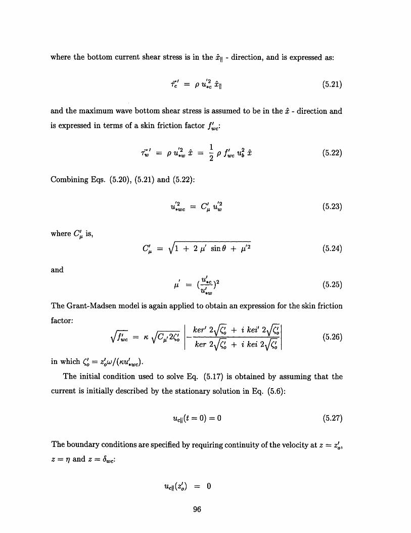
where the bottom current shear stress is in the Xll - direction, and is expressed as:

-#l12 -ilrc =P U*c X11 (5.21)

and the maximum wave bottom shear stress is assumed to be in the i - direction and

is expressed in terms of a skin friction factor fIC:

-# = 1'2 1-.2=^2

(5.22)

Combining Eqs. (5.20), (5.21) and (5.22):

(5.23)S12 /u 2*WC Cý w

where C' is,

Ci=1+ 2 /I' sin + /t'2

I

= ( )2" *W

The Grant-Madsen model is again applied to obtain an expression for the skin friction

factor:

J-C= K cV'2C

in which (C = z,'/(• u',c).

The initial condition used to solve Eq.

ker' 2V + i kei' 2ker 2V' + i kei 2V'

(5.26)

(5.17) is obtained by assuming that the

current is initially described by the stationary solution in Eq. (5.6):

uCl(t = 0) = 0 (5.27)

The boundary conditions are specified by requiring continuity of the velocity at z = z0,

z = 7r and z = 5•:

ll,(z.') = 0

and

(5.24)

(5.25)

UCiH(7-) = olCl(W) (5.28)

UC1l (c5;) = uC1 (b6c)

and continuity of the shear stress at z = and z = 6,,c:

[a u11 [ucIIl- Oz 8z,

(5.29)

S e C9iweAt the free surface the shear stress is assumed must be zero:

8u] = 0 (5.30)

5.2 Model Solution

5.2.1 Determination of the initial flow uoc

It is assumed that the near-bottom orbital velocity Ub and the frequency w are known.

The current can be specified in terms of the current shear velocity u,e and the apparent

roughness zoa. These parameters are obtained by fitting a logarithmic velocity profile

in the region z > 6,, to the time average velocity in the perpendicular direction.

Expressing the perpendicular component of the velocity for z > 5we as:

UCJ = u** In(z- ) (5.31)

comparison between Eqs. (5.14) and (5.31) give:

cos 0

Zoa = Zoal (5.32)

For a complete characterization of the initial flow it is necessary to calculate u,*W to

express the velocity in the region inside 3,w. For this purpose, an initial value of the

friction factor fw, = 0.2 is used to obtain u., = ufwc/2Ub and the Grant-Madsen

model is applied as follows:

i) tio = (uC/uW) 2

ii) C, = 1 + /o

iii) u'Ce = U*W

iv) Sc = 2 u,*wc/

v) Zo = 6JC(f )u.W/u./

vi) fwc(zo) by solving Eq. (5.12)

vii) u*, = fwc/2 Ub

viii) The new estimate of uw obtained in vii) is used to calculate a new value of o-,.

The steps from i) to vii) are repeated until convergence in /o is achieved. The final

values of uw, and zo are used in Eqs (5.14) and (5.15) to express the initial mean

flow in the perpendicular and parallel directions, respectively. The evaluation of the

friction factor fwc in step vi) was done by using an approximate explicit equation

derived from Eq. (5.12) by Madsen (1994).

5.2.2 Determination of ull(t)

The non-oscillatory time-dependent part of the parallel component of the velocity is

described by Eqs. (5.17) to (5.19). As the eddy viscosity in the lower region of the

flow z < r depends on u' w, which is obtained as part of the solution an iterative

procedure similar to the one described above is required. It is assumed initially that

uC, = 0, i.e L' = 0, and zo' is known. For the experiments with beads the value of

z', = d/30 and for the experiments without the beads the bottom roughness due

to skin friction is assumed to be the one corresponding to smooth turbulent flow,

1z = v/(9 u'e,). The solution of ucll(t) is obtained as follows:

i) CO = V1 + 2z'sin0 + p' 2

ii) fwc(z,) by solving Eq. (5.26)

iii) u, = f/2 Ub

iv) 'w = /U~/ '

v) Solve Eqs. (5.17), (5.18), (5.19) subject to the initial and boundary conditions

specified in Eqs. (5.27) to (5.30) at the given time tb/2 defined in Eq (4.10).

vi) Evaluate the current shear stress at the bottom, Tr = p K u~,cz au, 111/z at

z = z' and at t = tb/2.

vii) Obtain u'c = p

viii) Obtain i' = (u,/u',")2 with the estimates of u', and u', calculated in steps iii)

and vii) respectively. The steps i) to viii) are repeated until the value of pL' converges.

The Eqs (5.17), (5.18), (5.19) and (5.27) to (5.30) were solved numerically by using

a finite difference method and time stepped with a standard explicit Euler scheme as

explained in Appendix B. The numerical scheme for waves and currents differs from

the one used for the pure current case by the addition of the intermediate region

between ri < z < 4c. To evaluate the friction factor fwc in step ii) the explicit

equation for (5.26) derived by Madsen (1994) was used.

5.3 Comparison with the experiments

Measurements of the velocity profile were obtained when second order Stokes waves

of T = 2.63 sec and an amplitude of ; 6 cm were superimposed to the current. The

ripples were placed at 450 with respect to the incident flow. The measurements were

done only at the center of the flume, y = b/2, and at three locations along the I - axis:

over the trough between two ripples and over both crests. These measurements were

performed without beads and with beads. The profiles of the first-harmonic wave

amplitude and phase obtained in the wave-current experiments are shown in Figures

5-1 and 5-2. Figure 5-1 corresponds to the experiments with beads and Figure 5-2 to

the experiments without beads. The profile measured over the trough between two

ripples is indicated by 'o', the profiles measured over the crests are indicated by '.'.

The first harmonic wave amplitude of the U(1) - component of the flow is shown in

part (a) of each figure. The profiles present similar characteristics to those measured

102

101

10 15U(1) (cm/sec)

0 0.1phase

0.2of U(1)

10

·I fnIV

1 2V(1) (cm/sec)

101

10 0

in.

0.3Iv

3 4

2 4phase of V(1)

Figure 5-1: Wave amplitude and phase of the first harmonic obtained in the wave andcurrent experiments with beads. The measurements were performed at the center ofthe flume, y = b/2, and 0 = 450 . o: Profile over the trough .: Profile over the crestsa) U(1) b) V(1) c) phase of U(i) (radians) d) phase of V() (radians). The phasesare plotted relative to the phase of U(1) measured at z = 50 cm. The horizontal linesrepresent the ripple height and the wave boundary layer thickness

100

a) O

/0

O

OO0

o. O.( b)

o oo0

o 0OO

102

10,

I4 tA.IU

5

102

loo

C)

.·

O*O *

00

00O *

OO

O

d)

0.0d

- 0 000o

IV-0.1

|

A

L. :)

A S

L_

101

106

i 1

10 15U(1) (cm/sec)

0 0.1 0.2phase of U(1)

Iv0

102

10

0.3 0.4

10"

10

2 4V(1) (cm/sec)

0 2 4phase of V(1)

Figure 5-2: Wave amplitude and phase of the first harmonic in the wave and currentexperiments without beads. The measurements were performed at the center of theflume, y = b/2, and 0 = 450 . o: Profile over the trough .: Profile over the crests a)U(1) b) V1) c) phase of U(1) (radians) d) phase of V(1) (radians). The phasesare plotted relative to the phase of U(1) measured at z = 50 cm. The horizontal linesrepresent the ripple height and the wave boundary layer thickness

101

a) . O .

S.00

O

o* *O* b)

_ O.. O O0 00 0 00%,

102

10

10

1IV 1

IU

101

107

10-10

c)

0 0*00 O

0 0o00

·

----

AAR m

L-

r-

A n

in the pure wave experiments presented in Chapter 3. The effect of the individual

bottom roughness elements is felt up to a height of z z 4 cm. The gradients in the

U(1) - component extends to an elevation of z - 6 cm suggesting that the thickness

of the wave boundary layer is between 4 to 6 cm above the bottom.

Part (b) of each figure shows the first harmonic amplitude of the V(1) - component.

Close to the bottom it presents a value of approximately 3 to 4 cm/sec and it starts to

decrease when z increases. For elevations larger than 4 cm it remains approximately

constant until z x 20 cm where it starts to increase.

The time-average velocity profiles of the perpendicular component of the velocity

obtained in the experiments with beads and without beads are shown in Figures 5-3

(a) and 5-4 (a). A change in the slope of the profile is observed at at a height of 4

cm above the bottom.

These observations suggest that the wave boundary layer is at an elevation of

z e 4 cm measured from the bottom of the flume. The predicted wave boundary

layer thickness 6,, = 2u,,,w/w obtained after applying the Grant-Madsen model

as explained in section 5.2.1 is of the order of 2.5 cm, i.e. considerably smaller than

the value observed in the experiments. To take into account the enhanced boundary

layer, it was decided to follow Mathisen and Madsen (1996) and modify the the Grant-

Madsen model by replacing the predicted wave boundary layer thickness by the one

observed in the experiments. For the experiments with beads the theoretical bed is

defined at 0.35 times the bead diameter (d =0.64 cm) below the top of the beads.

Therefore the wave boundary thickness used in these experiments was Jw. = (4 -

0.65 *.64) cm. For the experiments without beads the wave boundary layer thickness

used was J,, = 4 cm.

Energy attenuation measurements were performed for the combined wave-current

experiments with and without beads when 0 = 450. The amplitude of the incident

wave obtained in the attenuation experiments were used to estimate the near-bottom

orbital velocity. For the experiments with beads Ub = 16.72 cm/sec and for the

experiments without beads ub = 16.64 cm/sec. These estimates of Ub were used as

input to the model.

102

Table 5.1: Input parameters to the Grant-Madsen model used to obtain the initialflow : Ub, Uc -= Lc COS 0, Zoa = Zoal, we ; 4 cm. Output parameters: uW,,uw,fwee and zo

Ub(cm/sec) U*c(cm/sec) U*WC (cm/sec) fwe *wc(cm/ec) U*c(cm/sec) tb/2(sec)

Beads 16.72 2.73 5.83 0.06 2.87 1.59 12.82No Beads 16.64 2.97 7.84 0.03 2.19 1.35 13.70

Table 5.2: Input parameters to the extended model for waves and currents :ub, ucand u*,. Output parameters: f'c, uW, uC;, tb/2

The current specification used as input to the model, uc and zoa, were obtained

from Eq. (5.32) after fitting a logarithmic velocity profile to the measurements of the

perpendicular component of the velocity in the region 4 < z < 9 cm . The input and

output parameters to the model are summarized in Table 5.1. The values obtained for

u,*w and zo were then used in Eq. (5.14) and plotted together with the experiments

in Figures 5-3 (a) and 5-4 (a). The predicted profile inside the wave boundary layer

obtained by applying the Grant-Madsen model with the modified wave boundary

layer agrees fairly well with experiments down to z = i7 and is used to describe the

initial flow.

Having defined the initial flow, Ucll(tb/2) is obtained following the procedure de-

scribed in section 5.2.2. The input prescribed to run the model were Ub, zo, u•e and

uwc. They are summarized in Table 5.2. Knowing ucll(tb/2), the component of the

velocity in the ^ - direction and Y - direction are obtained:

U(tb/2) = Ull(tb/2) sin9 + uo0 cos0 (5.33)

V(tb/2) = U11(tb/2) COS0 - uoc1L sine (5.34)

where Ull(tb/2) = u, 11 + Ull(tb,/2), uocll and uo0, are given in Eqs. (5.14) and (5.15),

103

5 10 15U-perpendicular (cm/sec) U-parallel (cm/sec)

102

1N"

0

0 5 10 15 20U (cm/sec)

I-5-5 0 5V (cm/sec)

Figure 5-3: Time average velocity profiles measured at the center of theb/2, in the wave and current experiments with beads for 0 = 450 a) Uj±and d) V.

flume, y =b) UI c) U

104

101

10,

I fl 1IV U

0

1%

Sn 2

I

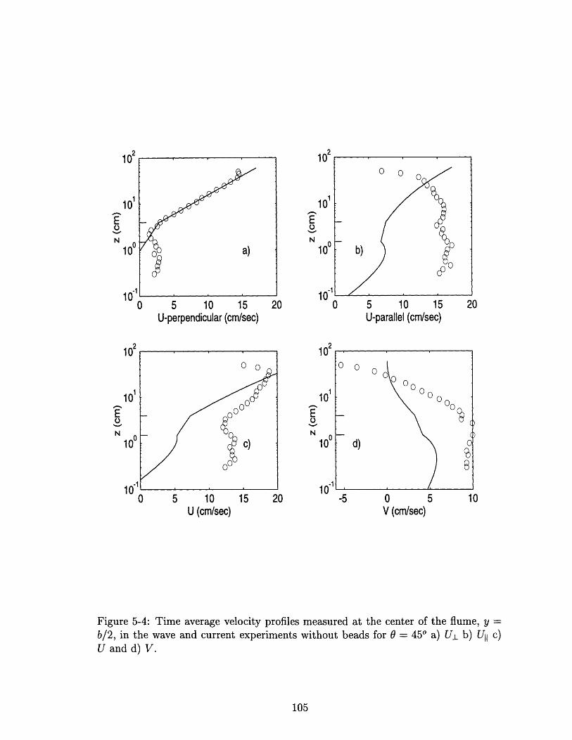
U-perpendicular (cm/sec)

5 10U (cm/sec)

102

101

100

15 20 -5 0 5V (cm/sec)

Figure 5-4: Time average velocity profiles measured at the center of the flume, y =b/2, in the wave and current experiments without beads for 0 = 450 a) UL b) U11 c)U and d) V.

105

102

101

100

-10

.- 2

U-parallel (cm/sec)

respectively. The predicted Ull(tb/2), U(tb/2) and V(tb/2) are plotted together with the

experimental results in Figures 5-3 (b), (c) and (d), respectively, for the experiment

with beads, and in Figures 5-4 (b) ,(c) and (d), for the experiment without beads.

The symbols represent the experiments and the solid line the predictions.

The predictions for the case of the experiments with beads presented in Figure 5-3

underestimate the measured profiles but qualitative agreement between theory and

experiments is observed. The experiments show a change in the slope both at z = rl

and at z = 6e, a feature reproduced by the predicted velocity.

For the experiment without beads the predicted profiles are not in good agreement

with the measurements. The experimental profile presented in Figure 5-4 (d) show a

large value of the V - component of the flow of about 10 cm/sec in the region z < 4

cm. The proposed model is based on a force concentrated close to the bottom which

drives the fluid along the ripple axis. The finite time t < tb/2 is not enough to advect

the flow in the region far from the bottom. The solution of the model is basically

a correction of the initial flow in the region close to the bottom. Comparing the

experimental profiles of the perpendicular and parallel components of the velocity it

is clearly seen that U1I does not present the same characteristics as U1 in the region

z > 6we. Eqs. (5.14) and (5.15) indicate that for the particular case of 0 = 450

the initial flow in the perpendicular and parallel direction are the same. Therefore a

correction close to the bottom will not be able to reproduce the measured UII.

The extended model is able to describe the near-bottom flow observed in the

experiments with beads only qualitatively but it fails in describing the experiments

without the beads. We are not too concerned about the relatively poor performance

of the model for this case, since it (as mentioned before) does not correspond to a

physically realistic flow condition.

106

Chapter 6

Model for Wave-Current Flows

Over Two-dimensional

Wave-Generated Ripples

In this chapter the information provided by the experiments is used to develop a

model able to describe the wave-current interaction problem in the field. The wave

characteristics are assumed to be such that the bottom topography consists of well

defined two-dimensional ripples and sediment transport is neglected. The current is

incident at an angle ~0, with respect to the waves as shown in Figure 6-1 The pure

current experiments described in Chapter 3 have shown two important aspects of the

near-bottom flow that results when the current is incident at an angle to the ripple

crest. First, the flow close to the bottom is turned towards the ripple axis; second ,

the bottom roughness depends on the angle between the ripple axis and the incident

flow. From the analysis of the velocity profiles in the direction perpendicular to the

ripple axis it was concluded that the bottom roughness experienced by the flow in this

direction is dominated by form drag and does not depend on the angle, whereas the

bottom resistance experienced by the flow in the direction parallel to the ripple axis

is associated with skin friction. Based on these conclusions, a wave-current boundary

layer model is proposed and compared to laboratory and field experiments.

107

__

Ripples

Waves I w.4 'CLL"/

;t

Current

Figure 6-1: Schematic definition of the angle between the direction of the wave prop-agation and the current.

6.1 Model

The model is basically the wave-current boundary layer model proposed by Grant and

Madsen (1979 and 1986) modified to incorporate the effects arising from the current

being incident at an angle to the ripple axis. The coordinate system is defined based

on the ripple axis and is shown in Figure 6-2, where £L is the direction perpendicular

to the ripple axis, and ^11 is the direction parallel to the ripple axis. Since it is

assumed that waves are responsible for the generation of the bedforms, the waves

are in the ^± - direction and are specified by their equivalent near-bottom orbital

velocity, Ub, and a period, T = 27r/w, as suggested by Madsen (1994). The current

is driven by a uniform pressure gradient in the ^ - direction defined by the angle 0,measured with respect to the ^I - direction. The magnitude and direction of the

pressure gradient is in principle unknown and is found after solving the problem.

In the Grant-Madsen model, the wave-current interaction takes place inside a thin

layer near the bottom defined as the wave boundary layer of thickness 6,,. Above the

wave boundary layer, the turbulence is only associated with the current. Assuming the

scale of the bottom roughness to be small compared to the boundary layer thickness,

the convective acceleration terms in the governing equation can be neglected and the

108

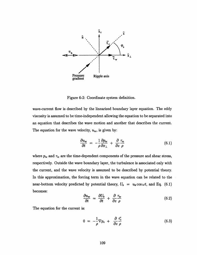
xil

1n .

Ub~---~---------s

s

10

Pressure Ripple axisgradient

Figure 6-2: Coordinate system definition.

wave-current flow is described by the linearized boundary layer equation. The eddy

viscosity is assumed to be time-independent allowing the equation to be separated into

an equation that describes the wave motion and another that describes the current.

The equation for the wave velocity, uu, is given by:

a1= p +1 9 (6.1)at p 8xI 8z p

where Pw and 7, are the time-dependent components of the pressure and shear stress,

respectively. Outside the wave boundary layer, the turbulence is associated only with

the current, and the wave velocity is assumed to be described by potential theory.

In this approximation, the forcing term in the wave equation can be related to the

near-bottom velocity predicted by potential theory, Ub =- UbCOSWt, and Eq. (6.1)

becomes:u, aUb a Twa = - + (6.2)Ot at Oz p

The equation for the current is:

1 8?0 = -VP +p Oz p

109

where pc and 7' are the time-independent components of the pressure and the shear

stress. Assuming that the current near the bottom is within the constant stress layer

Eq. (6.3) becomes:P = 2 , (6.4)

where u,, is the shear velocity based on the current bottom shear stress.

The results of the experiments described in Chapter 3 showed that the flow in

the direction perpendicular to the ripple axis experienced a roughness different from

that experienced by the flow in the parallel direction. Accordingly, the Grant-Madsen

model for the flow within the wave boundary layer is modified by assuming that:

i) The perpendicular component of the current shear stress, T•± = pu ,cos O ,

interacts with the waves accounting for the presence of the bedforms. The roughness

for the waves and the current in this direction are assumed to be given by a drag-form

resistance and will be denoted by z,,.

ii) The parallel component of the current shear stress, rc11 = PU2, sin 0,, interacts

with the waves as if the bottom were plane. The roughness for the waves and for the

current is assumed to be given by skin friction and will be denoted by z'.

As a result of the differences in roughness, the parallel component of the current

velocity near the bottom will be larger than the perpendicular component, producing

the current velocity to be turned towards the ripple axis with respect to the direction

defined by the angle 0,.

Inside the wave boundary layer the problem is solved by expressing the shear

stress in terms of an eddy viscosity. The eddy viscosity is assumed to be scaled by

the shear velocity based on the combined wave-current bottom shear stress. Because

the wave-current bottom shear stress is different in each direction, the eddy viscosity

representing the shear stress in the perpendicular direction will be different from the

one representing the shear stress in the parallel direction. In the direction perpendic-

ular to the ripple axis, the eddy viscosity is denoted by vt-, and the wave and current

shear stresses are given by:

T-- = t± (6.5)p 8z

110

-tl 9U, (6.6)p 8z

In the direction parallel to the ripple axis the eddy viscosity is denoted by vtll and

the current shear stress is expressed as:

ll = VIl (6.7)p az

The wave-current interaction problem is solved independently for the ij and Xll -

directions. The solution for the current velocity obtained inside the wave boundary

layer is then used to specify the boundary condition at 6 e, which is needed to solve

for the current velocity outside the wave boundary layer.

6.1.1 The solution inside the wave boundary layer:z < 6wc

Wave-Current interaction perpendicular to the ripple axis:^1 - direction

The flow in this direction is assumed to be rough turbulent and the bottom roughness

zo1 is assumed to be due to drag- form resistance. The eddy viscosity is assumed to

be given by:

Vt± = U*we z for z0o < z < 6,c (6.8)

where u,,, is the shear velocity based on the maximum bottom shear stress of the

combined wave and current flow. Introducing Eqs. (6.8) and (6.5) into (6.2), the

equation for the wave velocity:

O(U,- Ub) K a (uw - Ub)] (6.9)

at -z uz

and the equation for the current velocity in the perpendicular direction:

K uw,, z z - U,2 cos , (6.10),z

111

NOMMIW

Eqs. (6.9) and (6.10) with the boundary condition at the bottom:

uC±(ZoI) = 0

u,(Zo±) = 0 (6.11)

correspond to the solution of the Grant-Madsen model for the case when the waves

and currents are in the same direction. The thickness of the wave boundary layer is

defined as 6,, = 2tu,wc/w. The wave velocity for z < 6,w is expressed in terms of

the Kelvin functions of order zero:

u• -u•(1 -ker 2/V( + i kei 2 -Z7 e i t (6.12)

U ker 2v' + i kei 2/ )(1where ( = zw/Ku,,c and C(o is the value of ( at z = zo0 . The current velocity is

given by2 COS Z

ucI = *s In- (6.13)SU*wce zol

The solutions in Eqs. (6.12) and (6.13) are expressed in terms of ue,w which is

the shear velocity based on the maximum wave-current bottom shear stress in the

perpendicular direction, Twc±ma,, and is defined as:

Twc,,a, = PUwc = W,,, + T(6.14)

where Twa is the maximum wave shear stress at the bottom:

Twma = p I u~*e (6.15)

Defining u, = ýwma,/p to be the shear velocity based on the maximum wave

shear stress, Eq. (6.14) becomes:

2= , + u2cos, = (6.16)

112

where C, is:

C = 1 + icos5, (6.17)

and= (*8)2 (6.18)

The maximum wave bottom shear stress can be written as a function of a wave-current

friction factor defined as:

2 fWC 2TU)m,• = pu, = p U(6.19)

Combining Eqs (6.15) to (6.19) and using the series expansion of the Kelvin functions

Madsen (1994) obtained explicit equations to approximate the wave friction factor:

For 0.2 < Cub/(30 zo±w) < 102:

0(L0 C 8.820

fw = C, exp 7.02 )3078 - 8.82 (6.20)

and for 102 < CIub/(30 zoLw) < 104:

fW = c, exp 5.61 3 0.109 - 7.30) (6.21)30 z01w

Wave-current interaction parallel to the ripple axis: !I, - direction

In the direction parallel to the ripple axis the bottom roughness experienced by the

combined flow is assumed to be given by skin friction. If the flow is rough turbulent

the bottom roughness in this direction is zo = d/30 where d is the diameter of the

sediment. If the flow is smooth turbulent, the bottom roughness is zo = v/(9u',,),

where u',' is the shear velocity based on the maximum wave-current bottom shear,

ST$az. The criterion used to decide whether the flow is rough or smooth turbulent

is based on the value of the Reynolds number Re' = kbu*WC/v, where kb = d is

the equivalent Nikuradse bottom roughness. If Re' > 3.3 the flow is assumed to be

rough turbulent, otherwise the flow is smooth turbulent. This criterion corresponds

to choosing zo as the maximum value of d/30 and v/(9 u',,w). The maximum wave-

113

current bottom shear stress, Tcma:, is defined as:

'(12(.TwCmax = p U,. C = I Xjmax X-L_ + Tell Xlj (6.22)

where 7'•~ is the maximum wave bottom shear stress due to skin friction . The eddy

viscosity in the parallel direction Vtll is assumed to be given by:

r U'w z forz, < z <

t*ll = W(6.23)U*,wC z for 7 < z < 6we

where u,,w is the shear velocity based on the maximum wave-current bottom shear

stress obtained from the wave-current interaction in the perpendicular direction.

It must be noted that there is, in principle, another length scale to be considered.

It is the wave boundary layer thickness that represents the height to which turbulence

originating from skin friction diffuses away from the bottom. This wave boundary

layer is defined as 6w, = 2u'.wc/w. Scaling the Vjll with u'w up to the level defined

by the ripple height, is equivalent to assuming the thickness of the wave boundary

layer due to skin friction, 6w,, extends up to z = 77. In principle, this is not

necessarily true. For the case when 6'c < 77, it is assumed that the shear stress is

still represented by u'h w in the region between 6~, < z < 'q.

In the region defined by z' < z < 77, the wave velocity is denoted by u',. The

equation that describe the wave velocity in this region of the flow, u',, is the same

as Eq. (6.9) when u,, Ub and u,,, are substituted by u'., U and u,, respectively.

Accordingly, with the definition of vtll in z' < z < 77, Ub is obtained by evaluating the

solution for the wave velocity given in Eq. (6.12) at z = 77:

( ker2Jl + ikei2XJ \ 1UV = ub cos(wt + (,r) = 2v + ikei 2uv R 1 e -t (6.24)ker 2,\/-(Oj + i kei 2f)

where 7n = w/U*W,, u/ and ýo, are the amplitude and the phase of the velocity

at z = r.

114

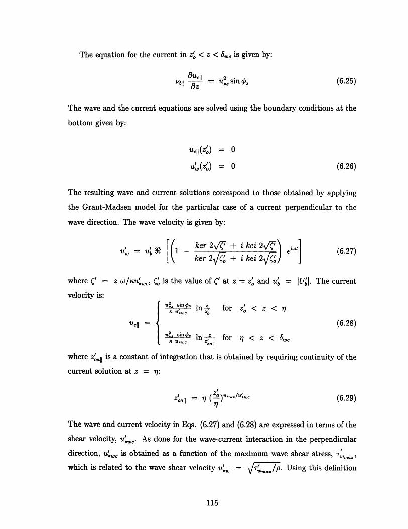
The equation for the current in z, < z < J., is given by:

aucl U sinV •ll 2 s,*sin 8u 8 z_ - ,

(6.25)

The wave and the current equations are solved using the boundary conditions at the

bottom given by:

l0(z') = 0u (z,)= 0 (6.26)

The resulting wave and current solutions correspond to those

the Grant-Madsen model for the particular case of a current

wave direction. The wave velocity is given by:

obtained by applying

perpendicular to the

I = ubjJ t -ker 2V(7 +

ker 2v( +

where (' = z w/snuw, I" is the value of (' at z

velocity is:

= z' and u- = IUll. The current-- bb

S* 'sin" In -L for z' < z < 71

ucll =0 (6.28)u*, sin~, In~- for 7 < z < 6,w

where z',,l is a constant of integration that is obtained by requiring continuity of the

current solution at z = 71:

(6.29)Z'.1= 77 (o0)tL*wc/t4'wc77

The wave and current velocity in Eqs. (6.27) and (6.28) are expressed in terms of the

shear velocity, ,u',. As done for the wave-current interaction in the perpendicular

direction, u',, is obtained as a function of the maximum wave shear stress, •-Wm,'

which is related to the wave shear velocity u',, = •~m•/p. Using this definition

115

i kei 2VJ

i kei 2ý )eiwt] (6.27)

in Eq. (6.22):

'2 '•U + U S, I2 '2u*WC *W+* s in '*8 =C,

where C' is:

0=JVj + Sin

and

S= (U*)2)

u*W

The maximum wave bottom shear stress is given by:

S[i

and can be written as a function of a wave-current friction factor based on skin friction

defined as:

*'2 w '2 (6.34)

where f , is expressed as in Eqs. (6.20) or (6.21) but replacing zox, Ub and C, by z•,

u' and C , respectively.

6.1.2 The solution outside the wave boundary layer: z > S6w

Outside the wave boundary layer the eddy viscosity is assumed to be:

v4t = r U*s Z (6.35)

and the current shear stress:it-

= vtp 9z

(6.36)

The current velocity u', in the (s, i)- coordinate system shown in Figure 6-2:

uc = U,8 + Un i (6.37)

The solution for the current outside the wave boundary layer is obtained by combining

116

(6.30)

(6.31)

(6.32)

(6.33)

( UIF

n

A

xI

Figure 6-3: The current velocity at z = 6we

Eqs. (6.37), (6.36), (6.35) and (6.4), and is given by:

U,*s zs = In

K zos

un = constant (6.38)

The value of the constants zos and un are obtained by requiring the current velocity

to be continuous at z = 6,,. The solution for the current velocity in the region

z < 6, was calculated in the previous section in terms of the perpendicular and

parallel components. Relating u,(65W) and u~ to u±(6,c) and ull(6wc) we obtain with

the aid of Figure 6-3:

U*S 6weus(6wc) = u1 cos ~, + ull sin = u In n

un = -u 1 sin , + u11 cos S (6.39)

with the expression for zos:

Zos = 6wc exp(-u,(6wc) K/u,s) (6.40)

117

c(zr)

AXIXL

Figure 6-4: The current velocity and the angle 0, at zr > 5,,

Finally, the current at a given z = z, > J6. is obtained in terms of (u,(zr), un), as

indicated in Figure 6-4:

uc(z,) = us(z,) cos¢, + u, sin¢q (6.41)

where 0,, the angle between the current at z = z, and the 9-direction, is given by:

tan Cr Un(Us(zr)

(6.42)

As u, is constant, using the expression for us from Eq. (6.38) in Eq.

current velocity at a given height can be written as a 'logarithmic' velocity profile:

uc(zr) = u,*r ln(r )K; Zoar

(6.43)

where u,. r and zoar are the current shear velocity and the apparent roughness, and

are given by:

u*cr = U*8 Cosor (6.44)

118

(6.41), the

I

A

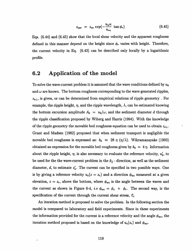
zoar = zos exp(-u tan ,Or) (6.45)u*s

Eqs. (6.44) and (6.45) show that the local shear velocity and the apparent roughness

defined in this manner depend on the height since 0, varies with height. Therefore,

the current velocity in Eq. (6.43) can be described only locally by a logarithmic

profile.

6.2 Application of the model

To solve the wave-current problem it is assumed that the wave conditions defined by Ub

and w are known. The bottom roughness corresponding to the wave generated ripples,

z, 1, is given, or can be determined from empirical relations of ripple geometry . For

example, the ripple height, r, and the ripple wavelength, A, can be estimated knowing

the bottom excursion amplitude Ab = Ub/w, and the sediment diameter d through

the ripple classification proposed by Wiberg and Harris (1994). With the knowledge

of the ripple geometry the movable bed roughness equation can be used to obtain zo-.

Grant and Madsen (1982) proposed that when sediment transport is negligible the

movable bed roughness is expressed as: kb 28 r7 (7/A). Wikramanayake (1993)

obtained an expression for the movable bed roughness given by kb = 4 rq. Information

about the ripple height, 7, is also necessary to evaluate the reference velocity, u', to

be used for the the wave-current problem in the Xll - direction, as well as the sediment

diameter, d, to estimate z'. The current can be specified in two possible ways. One

is by giving a reference velocity u,(z = zr) and a direction ewe measured at a given

elevation, z = zr , above the bottom, where k is the angle between the waves and

the current as shown in Figure 6-4, i.e €• = 4, + ~,. The second way, is the

specification of the current through the current shear stress, iF.

An iteration method is proposed to solve the problem. In the following section the

model is compared to laboratory and field experiments. Since in these experiments

the information provided for the current is a reference velocity and the angle 0"', the

iteration method proposed is based on the knowledge of uc(zr) and 0wc.

119

The number of unknowns in the problem can be reduced to four: 1) us,, 2) u

3) u,, and 4) ,r. The solution of the problem is divided in two parts. In the first

part, which is called "Iteration on u,(z,)", the solution for the waves, i.e, u,,w and

u',/, and the shear velocity u,, are calculated. In the second part, the angle 0, is

obtained. This part is called "Iteration on 0."

It is assumed initially that ,5. = 0, i.e, 0. = -b 1 and u,, is obtained based on the

given value of the reference velocity uc(Zr) as: u,, = uc(zr)h/ ln(zr/zo,), where z,,o

is an estimate of the apparent roughness which is assumed to be z,, = 10 77/30, i.e

larger than zjo = 4 r7/30 .

With these assumptions the problem is solved following the steps enumerated

below:

6.2.1 Iteration on Uc(zr)

In this part 0, is given and remains constant throughout the iteration. The goal is

to obtain uwc and ~u' which are needed to evaluate the parameters to calculate

uc(zr). The value of uc(zr) obtained is compared to the given reference velocity. The

process of iteration starts by assuming = -/ = 0:

Solve the wave-current interaction in 1± - direction:

Knowing ub, w and zo1 obtain uC.

i) C, = 1+ I cos0,

ii) f = f,,wc(Cub/(zo±w)) using Eq. (6.20) or (6.21)

iii) uW = fc/2 Ub

iv) uWC = tlU w

v) bec = 2 iu, /w

vi) u, = Iu,(z = r)l using Eq. (6.12)

Solve the wave-current interaction in the ^11 - direction:

Knowing t4, w and z, obtain u,wc.

vii) C,, = 1 + 1 '2 sin 2

viii) f~ = f,'~(C,, u'/(Z'W)) using Eq. (6.20) or (6.21)

120

ix) , uw = fwc/2 u•x) ,U

Obtain the current velocity at z = J.c:

xi) zoall = 1n (Z/7)u*w.c/u'wc

xii) u 11(5c) = (u2 sin ,)/(Ku,*) ln(5•c/Zoal)

xiii) u±(5~e) = (u, cos 8,)/(Ku.wc) ln(6J,/zo±)

Obtain u, and zo,:

xiv) u, ( w5c) = u ((5Jc)cos , + u ll(6u) sin ¢,

xv) un = -u±(5,c) sin q, + ull(5c) cos O,

xvi) Zo, = b5 exp[-u s (&5,)r/u.,]

Obtain the current velocity at z = z,:

xvii) u8(z7) = *s ln(z,/zos)/l

xviii) uc(Zr) = U~(Zr) + Un

Obtain a new estimate of u,*:

xix) In this part of the solution the comparison between the calculated and given

reference velocity is made. If uc(zr) calculated in step xviii) is different from the given

current velocity Ucgiven(zr), then a new estimate of u*, is obtained from:

U*Snew = gn - nr/ln(zr/zos)

xx) The value of u*,,,. is used to obtain new estimates of pj = (u,,*n./u*W)2 and

S= (u*sn,e/u':) 2 and return to i).

The steps i) to xx) are repeated with the new values of p and p' obtained in xx)

until convergence on uc(zr) is obtained. At this point the problem has been solved

under the assumption that 0, = Owe, i.e, 4, =0.

6.2.2 Iteration on Or

After solving steps i) to xx) the parameters needed to calculate the angle r, are

known, so a new estimate of ', is obtained as:

xxi) Cr,,, = tan-'(un/us(zr))

121

If the value of qr,, is different from the old value of 0, then 0, is recalculated as:

XXii) knew = OWC - Ornw

The updated 0, is used in part 6.2.1 of the solution. The steps i) to xx) are

repeated until uc(zr) converges, and 0, is calculated another time in part 6.2.2. The

process ends when both values of uc(zr), and Or converge.

In part 6.2.1 of the iteration scheme it was considered that the solution has con-

verged if u,(zr) differs from the previous estimate only in the third significant digit.

It must be noted that this criterion of convergence is applied to the examples that

are considered in the following section, where the specified reference velocity are of

the order of 2 to 40 cm/sec.

In part 6.2.2 the criterion of convergence is based on the accuracy of the determi-

nation of the angle Owe ± 5F.

In steps vii) to x) the energy friction factor due to skin friction f', depends

on z'. For the cases of smooth turbulent flow, the explicit equation of f' in Eq.

(6.21) was not applied because Cu'/(30 z/lw) was out of the range of validity of

the approximation. In this case the implicit equation of fic obtained after combining

Eqs. (6.27), (6.33) and (6.34) was solved to obtain u',wc.

6.2.3 Implications of the Model's Predictions

In general, experiments performed in the field consist on measuring the flow velocity

in the region close to the bottom. The waves are specified by a representative near-

bottom orbital velocity and period, ub and T, respectively. The current velocity,

uc(z), and the angle between the waves and the current, ,,wc(z), are measured at

say four elevations above the bottom. The current is assumed to be logarithmic

and the current shear velocity and apparent roughness, u, and z,,, are obtained by

fitting a logarithmic velocity profile to the measurements. If the resulting correlation

coefficient is low, or if there is an angular inconsistency throughout the profile , i.e,

the variability of the angle Ow, measured at the different elevation is too large , the

data is rejected.

The model predictions of the current velocity in Eq. (6.43) and the angle r, in

122

Table 6.1: Predicted local current shear velocity, us,., apparent roughness , zoar,and angle, Or, vs. the height above the bottom. The velocities are in (cm/sec), theroughness in (cm) and the angles in (0)

Eq. (6.42) imply that u, might not be exactly logarithmic and that 0,, might not be

constant. To investigate the implications of the present model for the conventional

analysis of field data on near-bottom currents in the presence of waves we consider

a wave specified by a representative near-bottom orbital velocity Ub = 15.3 cm/sec

and period T=11.2 sec. The bottom topography is characterized by wave-generated

ripples of height r = 1.72 cm and the bottom roughness in the perpendicular direction

is taken as zox = 4r//30.The current is specified by the magnitude and direction of

the pressure gradient, u*,, and 0,, respectively. The model is applied assuming u,.

= 0.5 and 1 cm/sec, and 0, = 300 and 600. The results obtained after solving the

problem under the assumption of smooth turbulent flow are summarized in Table

6.1. The shear velocity and the apparent roughness depend on the height through

the angle Or defined in Eq. (6.42). As an illustration, the shear velocity, u,., the

apparent roughness, zoar, and the angle, Or, are evaluated at two different heights

above the bottom: zr = 10 and 100 cm. These values are listed in the table where

the subscripts 10 and 100 denote the height z, at which these values are calculated.

123

Case A B C DuS 0.5 0.5 1 18 ' 30 60 30 60

un 2.08 2.03 7.52 6.59Zo, 1.10 0.16 0.33 0.02

C00oo 6.05 8.27 16.15 22.45

uCrlO 0.40 0.47 0.75 0.92ucrloo 0.47 0.48 0.89 0.96zoaro 0.31 0.09 0.02 0.006Zoarioo 0.58 0.11 0.07 0.008Oro 36.5 21.6 41.4 22.8qrloo 20.1 14.3 27.7 17.1R 0.9997 1.0000 0.9997 1.000

U*,rf 0.44 0.48 0.83 0.94zoarf 0.45 0.10 0.04 0.008

The current shear velocity, the apparent roughness, and the direction of the current

show a dependence on the height above the bottom. The predicted profile of uc(z)

in each of the four cases considered, was fitted by a logarithmic profile in the region

between 10 cm < z <100 cm. Four points were used in the fitting. The resulting

shear velocity and roughness obtained from the fitting, u,r,f and zoar,,,, are presented

in the last two rows of the table. The corresponding correlation coefficients were R ;

1.0, indicating that the predicted velocity in the region considered can be regarded as

logarithmic. For cases A) and C) the shear velocity calculated at the two elevations

differ about 15%, and the difference of the bottom roughness calculated at the two

elevations is within a factor of approximately 2 and 3, respectively. This difference is

not very important considering that the apparent roughness appears in the expression

of the current velocity as an argument in the logarithmic function.

The difference of the angle 0r evaluated at the two elevations , A.r, is 160, 70,

140 and 60, for cases A) to D), respectively. The angle between the wave and the

current is 0,, = 0, + Or (Figure 6-4). In the example A) a difference Aqr of ; 150

indicates a difference A c of ; 150. This difference is bigger than the error in general

estimated of ±50 in the determination of w,, in field experiments. This result implies

that an angular inconsistency obtained by the instrumentation does not necessarily

mean an error in the measurement .

In order to have a better picture of how the predicted current velocity u' depends

on the magnitude and direction of the driving pressure gradient, u., and 0,, Eqs.

(6.13) and (6.14) are used in Eq. (6.39) to obtain an expression of u, as a function

of the angle 0,:u= , Zol sin 2 (6.46)

u, = e'-- In( , ) (6.46)K Zoall 2

where E = u.,/u.,,, and Zo'll = 77 (z'/r)u*wc/u"'c . Similarly, Eqs. (6.13) and (6.14)

are used in Eq. (6.39) to express zos as:

zos = [we (zfz /(ifL ] (6.47)

124

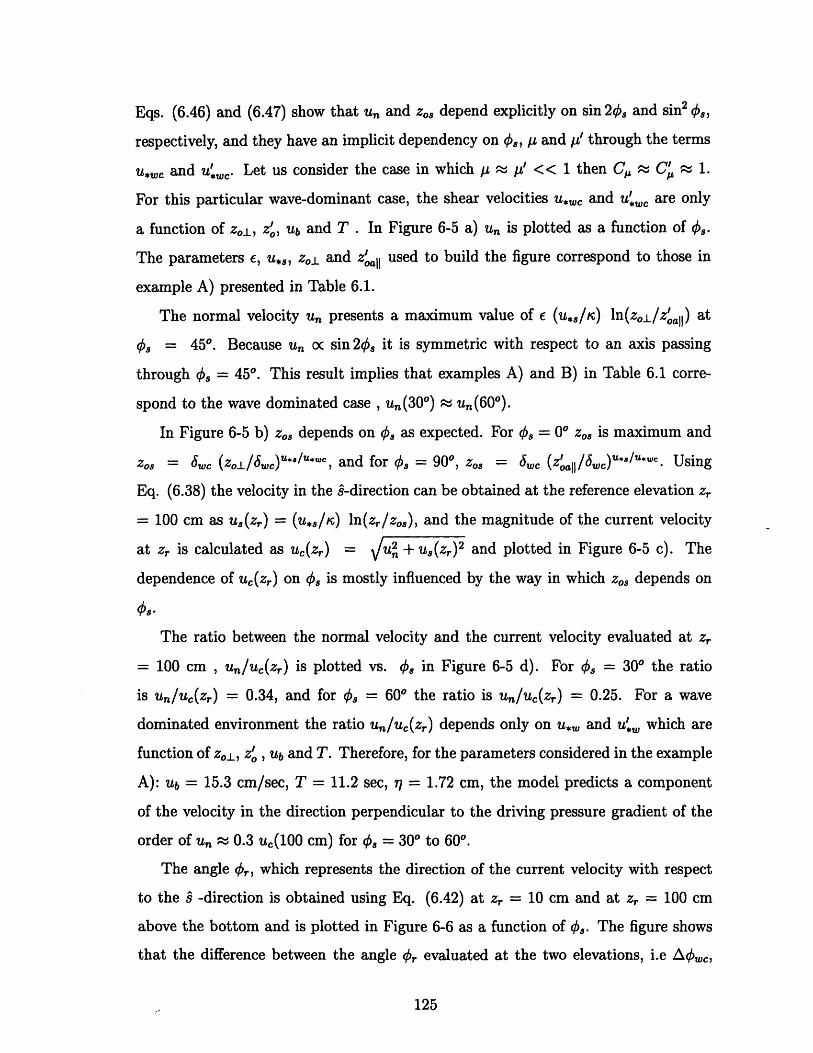
Eqs. (6.46) and (6.47) show that u,, and zo, depend explicitly on sin 20, and sin 2 €.,

respectively, and they have an implicit dependency on ~,, pt and p~' through the terms

uwc and u','. Let us consider the case in which pji I' << 1 then C, 0 C. - 1.

For this particular wave-dominant case, the shear velocities u,,, and u'uw are only

a function of zo, z7, Ub and T . In Figure 6-5 a) u, is plotted as a function of €,.

The parameters E, u, 8, zol and zoall used to build the figure correspond to those in

example A) presented in Table 6.1.

The normal velocity u, presents a maximum value of E (u,,/K) ln(zo±/z'al ) at

,8 = 450. Because u, oc sin 20, it is symmetric with respect to an axis passing

through q, = 450. This result implies that examples A) and B) in Table 6.1 corre-

spond to the wave dominated case , un,(300) • u,(600).

In Figure 6-5 b) zo, depends on 0, as expected. For 0, = 00 z,, is maximum and

zo8 = Jw~ (z0o/6W)" .)*/U*w ' , and for 0, = 900, z., = 6,w (z'all/6wc) *"/u*'W . Using

Eq. (6.38) the velocity in the i-direction can be obtained at the reference elevation z,

= 100 cm as u,(zr) = (u,,/K) ln(zr/zo,), and the magnitude of the current velocity

at zr is calculated as uc(zr) = u2 + uS(zr) 2 and plotted in Figure 6-5 c). The

dependence of uc(zr) on 0, is mostly influenced by the way in which zo, depends on

The ratio between the normal velocity and the current velocity evaluated at zr

= 100 cm , un/uc(z,) is plotted vs. 0, in Figure 6-5 d). For 0, = 300 the ratio

is un/uc(z,) = 0.34, and for 0, = 600 the ratio is un/uc(zr) = 0.25. For a wave

dominated environment the ratio u,/uc(z,) depends only on u,w and u', which are

function of zol, z' , Ub and T. Therefore, for the parameters considered in the example

A): Ub = 15.3 cm/sec, T = 11.2 sec, r7 = 1.72 cm, the model predicts a component

of the velocity in the direction perpendicular to the driving pressure gradient of the

order of u, P 0.3 uc(100 cm) for 0, = 300 to 600.

The angle 0,, which represents the direction of the current velocity with respect

to the ^ -direction is obtained using Eq. (6.42) at zr = 10 cm and at zr = 100 cm

above the bottom and is plotted in Figure 6-6 as a function of 0,. The figure shows

that the difference between the angle ,r evaluated at the two elevations, i.e Afc,

125

0.3

CO.1 5

C.1

o tl

10 20 30 40 .O O 70 BO C0phle

Figure 6-5: Magnitude of the predicted uc(Zr) vs. C, at zr = 100 m. a) u. (Eq.(6.46)). b) zos (Eq. (6.47)) . c) Uc(Zr) . d) u,/uc(Zr) .The '*' corresponds to caseA) presented in Table 6.1

126

G)

) 10 20 30 40 BO ~O 70 SO 9phll"

· ·- -- · · · ·

2.A

2.5

d)

>

0

s2m

is

o "o o o "o -o s-o s70 - o so

Figure 6-6: Angle 0, at ...: z, = 10 cm and at - Zr = 100 cm vs. q,. The '*'corresponds to the case A) presented in Table 6.1.

presents a maximum of A Pw- 0 180 when 0, P 200 . For the given wave conditions

and ripple geometry of example A) the variability of the angle between the waves and

current within 1 m above the bottom is expected to be A¢• x 15' for 0, = 300 and

nA¢ P,- 70 for 4, = 600 .

6.3 Comparison with experiments

The model described in the previous section is applied to the laboratory measurements

performed by Ranasoma and Sleath (1994) and to the field experiments performed

by Drake and Cacchione (1992) , Trowbridge and Agrawal (1995) and the field data

analyzed by Sorenson (1995).

6.3.1 Laboratory Experiments Ranasoma and Sleath (1994)

When the angle between the waves and the current is 0,, = 900, the proposed model

predicts that there is no wave-current interaction in the direction perpendicular to

the ripple axis. The interaction takes place in the direction parallel to the ripple axis

through the maximum wave-current skin friction bottom shear stress, 'r, a in Eq.

(6.22). To test this assumption the model predictions are compared to the laboratory

experiments performed by Ranasoma and Sleath (1994).

The oscillatory flow in these experiments was generated by oscillating a tray in the

127

zr-1~O om

A-ý

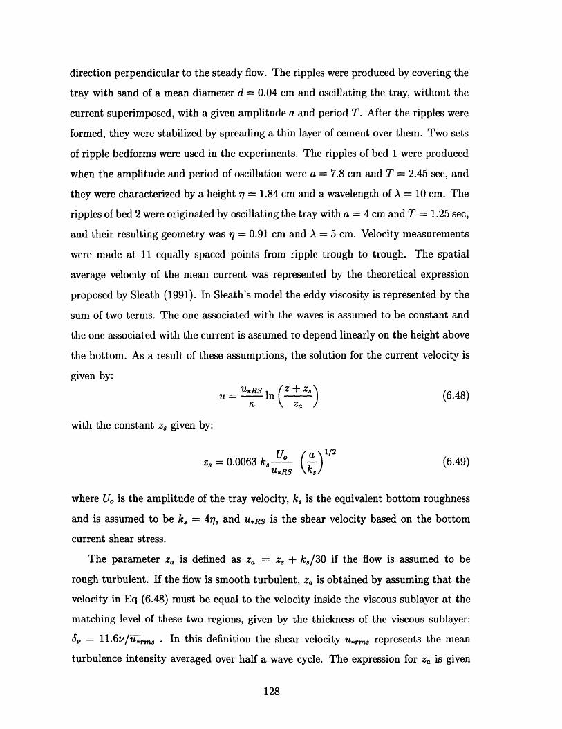
direction perpendicular to the steady flow. The ripples were produced by covering the

tray with sand of a mean diameter d = 0.04 cm and oscillating the tray, without the

current superimposed, with a given amplitude a and period T. After the ripples were

formed, they were stabilized by spreading a thin layer of cement over them. Two sets

of ripple bedforms were used in the experiments. The ripples of bed 1 were produced

when the amplitude and period of oscillation were a = 7.8 cm and T = 2.45 sec, and

they were characterized by a height 7r = 1.84 cm and a wavelength of A = 10 cm. The

ripples of bed 2 were originated by oscillating the tray with a = 4 cm and T = 1.25 sec,

and their resulting geometry was 7 = 0.91 cm and A = 5 cm. Velocity measurements

were made at 11 equally spaced points from ripple trough to trough. The spatial

average velocity of the mean current was represented by the theoretical expression

proposed by Sleath (1991). In Sleath's model the eddy viscosity is represented by the

sum of two terms. The one associated with the waves is assumed to be constant and

the one associated with the current is assumed to depend linearly on the height above

the bottom. As a result of these assumptions, the solution for the current velocity is

given by:

u s In Z +) (6.48)

with the constant z, given by:

U0 a\1/2z, = 0.0063 k, a(6.49)

U*RS \k/

where Uo is the amplitude of the tray velocity, k, is the equivalent bottom roughness

and is assumed to be k, = 47, and U*RS is the shear velocity based on the bottom

current shear stress.

The parameter za is defined as za = z, + k,/30 if the flow is assumed to be

rough turbulent. If the flow is smooth turbulent, za is obtained by assuming that the

velocity in Eq (6.48) must be equal to the velocity inside the viscous sublayer at the

matching level of these two regions, given by the thickness of the viscous sublayer:

J, = 11.6v/•,rm, . In this definition the shear velocity u,rm, represents the mean

turbulence intensity averaged over half a wave cycle. The expression for za is given

128

by:

Za (=z+ 105z08 )exp(-J 4 ) (6.50)

where

z8, = V/(9.05u.RS) (6.51)

and

C 1 + 0.017( -1/4 1/4 (6.52)

Several experiments are reported by Ranasoma and Sleath for both bedform geome-

tries. In Table 2 of their paper the test conditions: T and a, are listed, as well as

the value of U*RS obtained by a least squares fit to the measured velocity. The model

proposed in this chapter is applied to 6 of the experiments presented in the paper.

Except for the case of the test 109, for which the experimental velocity profile is

shown in figure 4 of the paper, the rest of the examples used in the comparison were

randomly chosen.

The period T and the amplitude of the tray velocity Uo = a 2 7r/T are used to

specify the waves. The bottom roughness in the perpendicular direction is estimated

based on the ripple geometry information as z0o = 4 r/30. The roughness used to

solve the wave-current problem in the 11 - direction is zo = d/30, i.e, the flow is

assumed to be rough turbulent in this direction because u'• , d/v > 3.3.

In order to apply the model the current reference velocity is obtained by using

the theoretical expression in Eq (6.48) evaluated at z, = 10 cm. For this purpose,

the parameter za has to be calculated. Two possible expressions are given for za

depending on the flow being smooth or rough turbulent. Based on the information

presented in the paper, it is inferred that the criterion used by the authors to decide

whether the flow is smooth or rough turbulent is based on the Reynolds number scaled

by 2 times the sand diameter, i.e., Re = 2 d *,Rs/v. The range of Re for which

the flow is considered to be smooth turbulent seems to be Re < 7 or a slightly larger

number.

The input parameters to the model are summarized in Table 6.2. In the last

129

Test a T Uo uc(z 7r) 77 U cr zoar U*RS Re(cm) (sec) (cm/sec) (cm/sec) (cm) (cm/sec) (cm) (cm/sec)

109 4.0 1.8 14.2 5.3 0.91 0.46 0.10 0.53 3.8114 4.0 2.5 10.3 13.7 0.91 0.78 0.01 0.88 6.1115 4.0 1.3 20.1 21.6 0.91 1.32 0.01 1.47 11.4

18 7.8 1.8 27.5 4.7 1.84 0.55 0.34 0.69 6.422 7.8 2.4 20.5 16.1 1.84 1.08 0.03 1.32 11.5

+23 7.8 2.4 20.3 13.8 1.84 0.97 0.04 2.05 18.923 32.7 1.74 0.05

Table 6.2: Model predictions and comparison with Ranasoma and Sleath (1994). u*,cand zoar are the current shear velocity predicted by the model. URS is the currentshear velocity obtained in the experiments and Re = 2duRs/IV

column of the table Re = 2 d *,Rs/V is presented. Assuming that the criterion

of flow condition classification used in the Ranasoma and Sleath's paper is Re < 7,

then only Test 109, 18 and 22 correspond to the case of smooth turbulent flow. Tests

number 114 and 22 have a Re 11, i.e., they have d U*RS/V M 6.5 close to the limit

of the smooth turbulent flow classification (Schlichting, 1968). For these tests the

reference velocity was calculated assuming that the flow was smooth turbulent and

Za was obtained by using Eqs. (6.50) to (6.52).

In Figure 6-7 (a) the experimental velocity profile for the test 109 of Ranasoma

and Sleath (1994) is represented by 'o'. The solid line corresponds to the predicted

velocity obtained after applying the present model. The dotted line is the theoretical

expression proposed by Sleath, Eq. (6.48). For this particular test, the present model

is able to predict the measurements.

The other examples listed in Table 6.2 were compared with the predicted velocity

by using the theoretical expression given by Eq. (6.48). The comparison between test

114, 115, 18 and 22 are shown in Figure 6-7 (b) to (e), respectively. The predicted

profiles are in agreement with the velocity obtained using Eq. (6.48).

The last 2 rows of the Table 6.2 correspond to the experiment 23. The value of Re

= 19 in Test 23 is high enough to consider the flow to be out of the smooth turbulent

region. In the row marked with a '+' the reference velocity uc(zr) = 32.7 cm/sec

130

100

10 - 1

u (cm/sec) u (cmrsec)

10'

N 10 0

10- 110(

10'

N 10

) # 22f) # 23

10 20 0 20 40u (crmsec) u (cm/sec) u (cm/sec)

Figure 6-7: Model predictions and comparison with the experimental work of Rana-soma and Sleath (1994).*: reference velocity o:experimental points .... :predictedvelocity given in Eq (6.48) -:present model prediction.

was obtained assuming that the flow was smooth turbulent. Using this reference

velocity in the present model, the predicted shear velocity u.,. is in agreement with

the measured shear velocity, uRs. The agreement is also observed in the profile

plotted in Figure 6-7 (f).

The model was also applied to Test 23 using the reference velocity obtained under

the assumption of rough turbulent flow, uc(zr) = 13.8 cm/sec. In this case the velocity

profile predicted by the present model does not agree with the velocity described by

Eq. (6.48). The corresponding plot is not presented, but the disagreement is reflected

in the predicted shear velocity ucr listed in the last row of the table. The values of

the reference velocity obtained for Test 23 by using Sleath's equations under the

assumption of smooth turbulent flow is uc(z,)=32.7 cm/sec, and the one obtained

under the assumption of rough turbulent flow is u,(zr) = 13.8 cm/sec. The difference

between the predicted references velocities is surprisingly large. The reference velocity

was calculated for other tests presented in the paper for which the Reynolds number

131

I

was close to the inferred transition region. The difference in the predicted reference

velocity under the assumption of smooth turbulent flow was unexpectedly larger than

the one obtained under the assumption of rough turbulent flow.

Due to the uncertainty in the criterion used to define whether the flow is smooth

or rough turbulent, it is concluded that the only truly valid comparison is the one

corresponding to test 109 for which the experimental velocity profile is presented in

the publication of Ranasoma and Sleath. The agreement between the experiment 109

and the prediction supports the assumptions made in the model for the particular

case of a current perpendicular to the wave direction.

6.3.2 Field Data from Duck.

Sorenson (1995), analyzed the data acquired by four electromagnetic current meters

placed on a tetrapod located on a 20 m isobath off Duck, North Carolina. The

shore-normal and shore-parallel velocity components were measured at four eleva-

tions, between 5 cm and 100 cm above the bottom. The measured time series were

analyzed to obtain the current velocity, uc, and direction, 0c, as well as the repre-

sentative near-bottom orbital velocity, Ub, the representative wave frequency, w, and

wave direction, 0,. Using or and .,, the acute angle between the waves and current

Owc was obtained. The bedform geometry was estimated based on the mean sediment

diameter, d = 0.018 cm, and the wave characteristics ub and w by applying the model

of ripple geometry proposed by Wiberg and Harris (1994). The bursts presented in

Sorenson (1995) number 115 to 125, and 127 are used in this section to compare

with the predictions of the model. The inputs to the model are the period T, the

near-bottom orbital velocity ub, the ripple height r7, the bottom roughness in the per-

pendicular direction, z,0o = 4 77/30, the sediment diameter d, the current reference

velocity at zr = 100 cm, ucr, and the angle between the wave and the current ,,c.

These parameters are listed in the first five columns of Table 6.3. The wave-current

interaction problem was solved following the procedure described in the previous sec-

tion. The predicted angle 0,, the current shear velocity based on the current shear

stress u,s, the current shear velocity velocity u,. (Eq. (6.44)) and apparent rough-

132

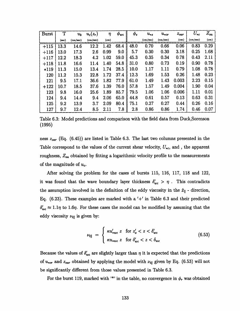
Burst T Ub uc(zr) ) 7 wc U• u, U*cr Zoar U*c Zoa(sec) (cm/sec) (cm/sec) (cm) (cm/sec) (cm/sec) (cm) (cm/sec) (cm)

+115 13.3 14.6 12.2 1.42 68.4 48.0 0.70 0.66 0.06 0.83 0.29+116 13.0 17.3 2.6 0.99 9.0 5.7 0.30 0.30 3.18 0.25 1.68+117 12.2 18.3 4.2 1.02 59.0 45.3 0.35 0.34 0.78 0.43 2.11+118 11.8 16.6 11.4 1.40 54.8 31.0 0.80 0.73 0.19 0.90 0.78*119 11.3 15.0 13.4 1.74 28.5 10.0 1.17 1.11 0.79 1.08 0.78

120 11.2 15.3 22.8 1.72 37.4 12.3 1.69 1.53 0.26 1.48 0.23121 9.5 17.1 36.6 1.82 77.9 61.0 1.49 1.43 0.003 2.23 0.15

+122 10.7 18.5 37.6 1.39 76.0 57.8 1.57 1.49 0.004 1.90 0.04123 9.8 16.0 25.6 1.89 85.7 79.5 1.06 1.06 0.006 1.11 0.01124 9.4 14.4 9.4 2.06 65.0 44.8 0.61 0.57 0.13 0.63 0.31125 9.2 13.9 3.7 2.09 80.4 75.1 0.27 0.27 0.44 0.26 0.16127 9.7 12.4 8.5 2.11 7.8 2.8 0.86 0.86 1.74 0.46 0.07

Table 6.3: Model predictions and comparison with the field data from Duck,Sorenson(1995)

ness Zoar (Eq. (6.45)) are listed in Table 6.3. The last two columns presented in the

Table correspond to the values of the current shear velocity, Uc, and , the apparent

roughness, Zoa obtained by fitting a logarithmic velocity profile to the measurements

of the magnitude of u,.

After solving the problem for the cases of bursts 115, 116, 117, 118 and 122,

it was found that the wave boundary layer thickness 6~ > r . This contradicts

the assumption involved in the definition of the eddy viscosity in the ill - direction,

Eq. (6.23). These examples are marked with a '+' in Table 6.3 and their predicted

6 , 1.17 to 1.677. For these cases the model can be modified by assuming that the

eddy viscosity Vtll is given by:

= { ,wt z for zo < z < 6w' (6.53)

tll * W (6.53)u*we z for 6', < z < w

Because the values of 6•' are slightly larger than ,7 it is expected that the predictions

of u*, and zoar obtained by applying the model with vtl given by Eq. (6.53) will not

be significantly different from those values presented in Table 6.3.

For the burst 119, marked with '*' in the table, no convergence in 0, was obtained

133

by applying the iteration method described in the previous section if ,r = 0 was used

as an initial guess. However a converged solution could be obtained if the value

OWC = 330 was used as an input, instead of the measured value 0,, = 28.50. This

converged solution predicts that r, = 20.70. The problem then was solved another

time using the measured value w,, = 28.50 as an input, but now with the value of

br = 20.70 obtained in the previous calculation as an initial guess. In this case, the

iterative method converged to a solution with the value 0, = 18.500.

This example illustrates that a good initial guess is sometimes required for the

iteration method to converge properly. In this example, it was possible to obtain

a converged solution only by first obtaining a better initial guess by running the

iteration program with a modified input variable. This implies that there are cases

where a solution exists but cannot be found at the first pass through the iteration

method.

As an independent check, solutions were found using a standard multidimensional

Newton-Raphson subroutine (Press et al, 1992) that solves an arbitrary system of N

nonlinear equations with N unknowns. The solution obtained with this subroutine

was found to be in perfect agreement with the one obtained by the proposed iteration

method.

In Figure 6-8 (a), the predicted and experimental shear velocities are compared

graphically. The predicted values of the shear velocity, u,., are indicated by '*'

and the measured, Uc, by 'o'. The dotted lines represent the error interval based

on the standard deviation of U.,. The predicted shear velocities, u,, , show good

agreement with the experimental shear velocity except for the cases of the bursts 121

and 122 where the theoretical shear velocity is smaller by a factor of F 0.7 relative

to the experimental values. The predicted apparent roughness, Zoar, is compared

with the experimental apparent roughness, Zoa, in a semilog-plot in Figure 6-8 (b).

The predicted values are indicated by '*' and the experimental by 'o'. The dotted

lines represent the error interval based on the standard deviation of In Zoa. The

agreement observed in the roughness is not as good as the one observed in the shear

velocities. The predicted apparent roughness is smaller by ; an order of magnitude

134

0O

U)

EO0

inI1lU

100

o -110

N

10-2

013115 120 125

Burst Burst

Figure 6-8: Model prediction and comparison with the field data of Duck. a) Currentshear velocity b) apparent bottom roughness

for the cases of the bursts 115 and 122, and, by two order of magnitude for the

case of burst 121. The predicted roughness for the burst 127 is bigger than the

measured by two orders of magnitude. The disagreement between the predicted and

measured apparent roughness becomes relatively smaller since Zoa is the argument of

the logarithmic function.

Clearly, there is some disagreement between the predicted and the experimental

shear velocity and apparent roughness. However, the proposed model still provides a

qualitative description of the effect of the angle between the wave and the currents

on the near-bottom flow.

Let us consider the cases of burst 120 and 123. These two bursts have similar

characteristics. Their waves are represented by a period of T f 10 to 11 sec and their

near-bottom orbital velocity by ub 15 to 16 cm/sec. The current reference velocity

is uc(z,.) , 23 to 26 cm/sec, and the ripple height q - 1.7 to 1.9 cm. The main

difference between these two cases is the angle between the wave and the current:

,vC = 370 and 800, respectively. The experimental current shear velocity and

apparent roughness listed in Table 6.1 is U.c = 1.5 cm/sec and Z,, = 0.2 cm for burst

135

NoO' b)

I I\

.\..

'.c

120 for which 0,c = 37' . For burst 123, U,c = 1.1 cm/sec and Zo,, = 0.01 cm.

This experiment has a €• = 800. A decrease in the current shear velocity and the

apparent roughness observed in burst 123 with respect to burst 120 can be explained

by the difference in angle between the waves and the current.

The conventional Grant-Madsen model (1986) was applied to bursts 120 and 123,

using the same inputs as the one used in the model described in this chapter: Ub,

T, uc(Zr) and the single-valued bottom roughness obtained as z0o = 4,q/30. The

predicted current shear velocity and apparent roughness obtained for burst 120 were

u,*M = 1.99 cm/sec and zo,,, = 1.02 cm, and for burst 123, the predicted values

were ucGM = 2.15 cm/sec and zoaGM = 0.81 cm. The results obtained by using

the Grant-Madsen model overpredict the experimental shear velocity and apparent

roughness. In addition, the estimated apparent roughness are of the same order in

both experiments and no angle dependence is predicted. These results are expected

because the parameters used in the model to solve the problem for the two examples

are of the same order, and, because the angle dependence in the formulation is given

by a p cos 0,, in the C, term. On the other hand, the predicted roughness obtained

by applying the proposed model are zo,,, = 0.26 cm for Burst 120, and Zo,, = 0.006

cm for Burst 123. The proposed model is able to reproduce the angle dependence

observed in the experiments.

The ability of the proposed model to reproduce the angle dependence of the appar-

ent roughness is based on the addition of a near-bottom velocity component parallel

to the ripple axis.

6.3.3 Field Experiments Drake and Cacchione (1992)

The model was also tested against the field experiments performed by Drake and

Cacchione (1992) on the inner shelf in northern California. Velocity measurements

were obtained with two -axes electromagnetic current sensors at three heights within

1 m above the bottom. During the period of the experiments the bottom topography

consisted of two set of ripples. The larger set of ripples, had an average wavelength

of A = 26 cm, and an average height of 7 = 3.5 cm. The second set of ripples

136

Test T Ub Uc(Zr) rl we Us U*cr Zoar U*c Zoa(sec) (cm/sec) (cm/sec (cm) (cm/sec) (cm/Sec) (cm) (cm/sec) (cm)

2 12.4 13.1 8.2 3.5 85.0 79.6 0.47 0.46 0.09 0.69 0.981 11.9 11.5 7.7 3.5 72.0 55.0 0.47 0.45 0.11 0.71 1.414 12.8 13.8 9.3 3.5 68.0 46.3 0.59 0.55 0.12 0.83 1.17

13 11.9 11.4 7.5 3.5 58.0 34.6 0.54 0.50 0.24 0.66 1.1212 13.2 10.0 8.0 3.5 55.0 29.9 0.58 0.52 0.23 0.71 1.169 11.6 10.7 8.3 3.5 48.0 23.4 0.65 0.59 0.38 0.77 1.50

Table 6.4: Model predictions and comparison with Drake and Cacchione (1992). Theroughness in the parallel direction is zo = v/(9u'.w,)

were developed within the troughs of the larger ripples. They were characterized by a

wavelength of approximately 8 to 12 cm and a height of 1 cm. The sediment diameter

was d= 0.025 cm and suspended sand concentration was found to be negligible.

The model was applied to 6 (randomly chosen) of the 23 experiments reported by

Drake and Cacchione. Assuming that the dissipation due to form drag is associated

with the largest ripples, the roughness in the perpendicular direction was obtained

as zo_ 77 rl (ar/A) 0.43 cm, which is approximately the value obtained by using

zo_ = 477/30 = 0.47 cm. The input used are Ub, T, Zo0 = 0.43 cm, the current

velocity Uc(z,) specified at z, = 1 m, the angle between the waves and the current

Cwc, and the ripple height 7r = 3.5 cm. These parameters are shown in the first

5 columns of Table 6.4. The estimated values of the angle ,S, the shear velocity

based on the current shear stress u,,, the current shear velocity u,r and the apparent

roughness zoa, obtained by applying the model are presented in Table 6.4. The last

two columns of this table correspond to the experimental current shear velocity U,c

and apparent roughness Zo, obtained by fitting a logarithmic profile through the three

measurements. The predicted shear velocity u,; z 0.5 cm/sec is lower than the one

observed experimentally which is of the order of Uc 0.7 cm/sec. The predicted

apparent roughness zo, also underestimates the value of Zo, by approximately an

order of magnitude.

The model is not able to predict these set of experiments quantitatively. Qualita-

tively, the predicted apparent roughness show the angle dependence observed in the

experiments, the smaller roughness corresponds to the larger ec. From the descrip-

137

----

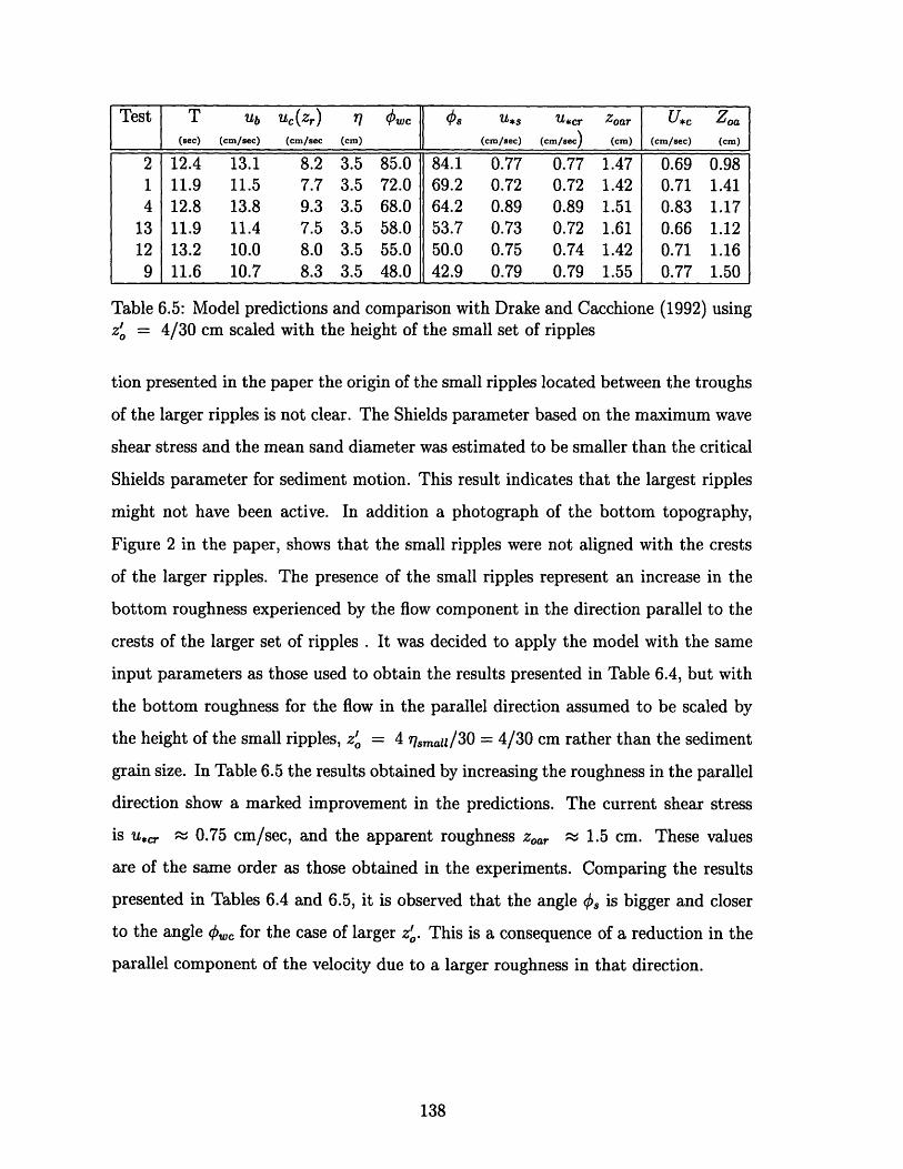
Test T Ub u,(zr) r7 wc ~ U*s u *cr Z oar ,. Zoa(sec) (cm/sec) (cm/sec (cm) (cm/sec) (cm/sec) (cm) (cm/sec) (cm)

2 12.4 13.1 8.2 3.5 85.0 84.1 0.77 0.77 1.47 0.69 0.981 11.9 11.5 7.7 3.5 72.0 69.2 0.72 0.72 1.42 0.71 1.414 12.8 13.8 9.3 3.5 68.0 64.2 0.89 0.89 1.51 0.83 1.17

13 11.9 11.4 7.5 3.5 58.0 53.7 0.73 0.72 1.61 0.66 1.1212 13.2 10.0 8.0 3.5 55.0 50.0 0.75 0.74 1.42 0.71 1.169 11.6 10.7 8.3 3.5 48.0 42.9 0.79 0.79 1.55 0.77 1.50

Table 6.5: Model predictions and comparison with Drake and Cacchione (1992) usingzo = 4/30 cm scaled with the height of the small set of ripples

tion presented in the paper the origin of the small ripples located between the troughs

of the larger ripples is not clear. The Shields parameter based on the maximum wave

shear stress and the mean sand diameter was estimated to be smaller than the critical

Shields parameter for sediment motion. This result indicates that the largest ripples

might not have been active. In addition a photograph of the bottom topography,

Figure 2 in the paper, shows that the small ripples were not aligned with the crests

of the larger ripples. The presence of the small ripples represent an increase in the

bottom roughness experienced by the flow component in the direction parallel to the

crests of the larger set of ripples . It was decided to apply the model with the same

input parameters as those used to obtain the results presented in Table 6.4, but with

the bottom roughness for the flow in the parallel direction assumed to be scaled by

the height of the small ripples, z, = 4 q.sma../30 = 4/30 cm rather than the sediment

grain size. In Table 6.5 the results obtained by increasing the roughness in the parallel

direction show a marked improvement in the predictions. The current shear stress

is u,,r 0.75 cm/sec, and the apparent roughness Zo,,a 1.5 cm. These values

are of the same order as those obtained in the experiments. Comparing the results

presented in Tables 6.4 and 6.5, it is observed that the angle 0, is bigger and closer

to the angle 0,, for the case of larger z',. This is a consequence of a reduction in the

parallel component of the velocity due to a larger roughness in that direction.

138

6.3.4 Field Experiments Trowbridge and Agrawal (1995)

The field experiments performed by Trowbridge and Agrawal (1995) at Duck, North

Carolina were used to test the model. The results of two experiments , called Glimpse

1 and Glimpse 2, are reported in their paper. Problems with the instrumentation did

not allow the measurements of the two components of the velocity during Glimpse 2,

therefore only Glimpse 1 is consider to test the model. The velocity was measured

at 4 elevations within 15 cm above the bottom with a laser Doppler velocimeter.

During the period of the measurements corresponding to Glimpse 1 it was observed

that wave-generated ripples with a wavelength A 10 cm were formed with the crests

placed perpendicular to the direction of wave propagation. The bottom consisted of

sand grains of diameter d = 0.02 cm.

The angle between the waves and the current was ,,w = 700, the waves were

specified by a representative near-bottom orbital velocity Ub = 15.8 cm/sec and period

T = 9.1 sec. The measurements of the wave amplitude and phase profiles were

analyzed based on the Grant-Madsen model (1986) to obtain the the wave-current

shear velocity, u,. = 2.31 cm/sec, and the bottom roughness , zo± = 0.044 cm. From

the analysis of the current velocity outside the wave boundary layer the current shear

velocity was estimated U., = 0.99 cm/sec, and the resulting apparent roughness was

Zoa = 0.56 cm. These values are listed in the last 2 columns of Table 6.6.

To test the present model it was assumed that the bottom roughness was the

one estimated by Trowbridge and Agrawal, zo± = 0.044 c. The ripple height was

calculated using the movable bottom roughness equation proposed by Grant and

Madsen (1982): q = 0.7 cm. The waves were specified by Ub and T and the current

reference velocity was assumed to be the velocity measured at the highest elevation zr

= 14.5 cm, uc(zr) = 7.7 cm/sec. The predicted current shear velocity and apparent

roughness, ucr and Zoar, obtained after applying the model are listed in Table 6.6 .

The predicted current shear velocity ,cr = 0.6 cm/sec is smaller than the measured

value Uc = 0.99 cm/sec. Similarly, the predicted bottom roughness zo., = 0.08

cm underpredicts the experimental value Zo, = 0.5 cm. Although the model is not

139

T Ub uc(z,) ~c U*, s U,, Zoa,. Uc Zoa(sec) (cm/sec) (cm/sec (cm) (cm/sec) (cm/sec) (cm) (cm/sec) (cm)

9.1 15.8 7.7 0.7 70 51.9 0.62 0.59 0.08 0.99 0.5Table 6.6: Model predictions and comparison with Trowbridge and Agrawal (1995)

able to reproduce the observations presented by Trowbridge and Agrawal (1995), the

agreement obtained between the result of the model and the available experimental

set of data is encouraging. Based on the results obtained from the data presented

by Sorenson (1995) good agreement beween the predicted and experimental shear

velocity was obtained in 9 cases out of 12 of the experiments analyzed. The most

remarkable feature of the model is its ability to reproduce the angle dependence of

the bottom roughness observed in the experiments.

140

Chapter 7

Conclusions

The purpose of this thesis has been to understand the nature of the near-bottom

flow produced under the combined effect of waves and current for the most general

situation where the current is incident at an angle to the waves. Because of the

constraints of the experimental setup, this problem was investigated experimentally

in a situation where both waves and currents are incident at the same angle to two-

dimensional artificial bottom roughness elements that simulate the wave-generated

ripples. The wave-current experiments performed deviate from the real situation in

the field where only the current is incident at an angle and the waves are perpendicular

to the ripples. Despite this limitation, the experimental results have yielded major

physical insights into the characteristics of the near-bottom flow that results from the

ripples being oriented with their axis at an angle to the incident flow. These results

provided the basis for the development of a general model capable of predicting this

flow quantitatively in the limited set of field experiments available.

7.1 Summary of Experimental Results

7.1.1 Pure Wave Experiments

Velocity measurements were performed for ripples placed at a 450 angle to the incident

wave. This first series of experiment led to the following conclusions:

141

__ _I

1) The velocity measurements presented in Chapter 3 show that there is a remark-

able difference between the profiles that describe the wave amplitude and the phase

of the components of the flow in the direction perpendicular and parallel to the ripple

axis. In the direction perpendicular to the ripple axis, a large wave boundary layer

thickness was observed in the profiles. This enhanced wave boundary layer indicates

larger turbulence intensities, and therefore a larger bottom roughness. On the other

hand, the flow in the direction parallel to the ripple axis exhibits a much thinner

wave boundary layer indicating that the bottom roughness experienced by the flow

in this direction is smaller than the one experienced by the component of the flow in

the direction perpendicular to the ripple axis.

2) Pure wave energy dissipation measurements were performed when the waves

were propagating over the rippled bed for 0 = 00, 300, 450 and 600. The energy

friction factor fe was estimated from the wave characteristics. The analysis of the

results indicates that fe is proportional to cos3 which suggest the value of the drag

coefficient Cd to be independent of 9 if the drag force is scaled by the square of the

reference velocity in the direction perpendicular to the ripple axis, Un,.

7.1.2 Pure Current Experiments

Velocity measurements were performed when the ripples were placed at 0 = 00, 300, 450

and 600. The main results obtained in the pure current experiments can be summa-

rized as follows:

1) The measurements presented in Chapter 3 indicate the presence of a compo-

nent of the velocity in the transverse (Y) direction. At the bottom, the value of the

transverse (V) component of the flow is of the same order as the longitudinal (U)

component. Further from the bottom, the V - component decreases and the U - com-

ponent increases. This observation show that the flow close to the bottom is turned

towards the direction parallel to the ripple axis.

2) The spatial average profiles show a well-defined logarithmic region within a

distance of approximately 7 cm above the bottom. The logarithmic region of the

flow was analyzed by fitting a logarithmic velocity profile by the least square method.

142

The shear velocity and bottom roughness were estimated. The results show that

the bottom roughness experienced by the component of the flow in the longitudinal

direction, zox, dep ends strongly on the angle of incidence 0, and is reduce

than one order of magnitude when 0 increases from O0 to 600. In contrast, the bottom

roughness obtained from the analysis of the component of the flow in the direction

perpendicular to the ripple axis, zo±, is independent of the angle 9.

3) The flow resistance experienced by the flow incident at an angle to the ripple

axis was expressed in terms of a drag force. The drag coefficient obtained is indepen-

dent of the angle of incidence if the drag force is scaled by the square of the reference

velocity in the direction perpendicular to the ripple axis at the elevation of the ripple

crest.

7.2 Simple models describing the experiments

In Chapter 4 the concept of a drag force oriented perpendicular to the ripple axis

is introduced in the formulation of a simple model to describe the near-bottom flow

observed in the pure current experiments.

In the model the bottom shear stress in the direction perpendicular to the rip-

ple axis is balanced by the drag force. The component of the shear stress in the

parallel direction to the ripple axis is initially unbalanced and is used to represent a

driving force that will induce the fluid to move along the ripple axis. The predicted

velocity profiles for the transverse velocity obtained with the simple model show good

agreement with the observations.

In Chapter 5 the model was extended to incorporate the presence of waves in the

direction of the current corresponding to the experimental conditions. The model

was able to predict only qualitatively the transverse velocity structure in experiments

performed with beads covering the bottom between roughness elements, but it failed

in predicting the wave-current experiments without beads.

143

_ ~I_

7.3 Model for waves and currents propagating in

different direction

In Chapter 6 the Grant-Madsen model (1979 and 1986) was modified to incorporate

the results observed in the experiments described in the thesis.

The proposed model assumes that the wave-current interaction depends on the

direction. The velocity measurements obtained in the experiments have shown that

the bottom roughness experienced by the component of the flow in the direction

perpendicular to the ripple axis is different than the one experienced by the component

of the flow in the direction parallel to the ripple axis.

Based on this observation, the Grant-Madsen model was modified by assuming

that the current component in the direction perpendicular to the ripple axis, i.e, in

the direction of the wave propagation, interacts with the waves accounting for the

presence of a wave-generated bedform. Therefore, the flow resistance is mainly due

to drag form. In the direction parallel to the ripple axis, the current interacts with

the waves as if the bottom were plane and the flow resistance is associated with skin

friction.

Due to the differences in the roughness, the component of the current veloc-

ity parallel to the ripple axis is relatively larger than the perpendicular component,

producing the current velocity to turn towards the ripple axis as the bottom is ap-

proached.

As a result of the model formulation , the current velocity outside the wave bound-

ary layer consists on two components. The component in the direction of the driving

pressure gradient behaves logarithmically. The other component, un, is in the direc-

tion perpendicular to the driving pressure gradient and is independent on the height

above the bottom. By adding the constant component, the current velocity behaves

quasilogarithmically, and the angle between the current and the direction of the wave

propagation ,€w, depends on the height above the bottom. An illustrative example

was presented in section 6.2.3 where the waves were represented by a near orbital

velocity ub = 15.3 cm/sec ,a period T = 11.2 sec and the ripple height was eta= 1.72

144

cm. For these particular conditions and under the assumption of a wave dominated

environment the normal component of the velocity is expected to be u, . 0.3 u,(z,=

1 m) when the angle between the waves and the driving pressure gradient, 0,, is

between 300 to 600.

The direction of the current outside the wave boundary layer depends on the

height. Within 1 m above the bottom the variability of the angle between the waves

and the current, AW C , was estimated for the case of a wave dominated environment.

It was obtained that A,, P-. 150 to 70 when the angle 0, varies from 300 to 600. The

maximum variability was found to be of the order of A0w, 18' when q, a 200. This

variability is bigger than the error in general estimated of ±5" in the determination of

0,we in field experiments. This result implies that an angular inconsistency obtained

by the instrumentation does not necessarily mean an error in the measurement .

Another consequence of the presence of a normal component of the velocity, un, is

that the angle between the waves and the current, 0,,, is different from the angle

between the waves and the direction of the driving pressure gradient , 0,.

The laboratory experiments of Ranasoma and Sleath (1994) were used to test the

model in the limiting case of wave and currents at a right angle. The velocity profile

predicted by the model show an excellent agreement with their Test 109. This result

supports the assumption that for the limiting case of waves and current at a right

angle there is no wave-current interaction in the direction perpendicular to the ripple

axis.

Available experimental field data presented by Sorenson (1995) was used to test

the model. Twelve experiments were analyzed in which the angle between the waves

and the current, e,,, varied between 800 to 100 approximately. It was further shown

that the present model was superior to the conventional application of the Grant-

Madsen model with a single-valued bottom roughness in representing Sorensons's

data. The ability of the present model to reproduce the angle dependence is based

on the addition of the near-bottom velocity component parallel to the ripple axis.

The proposed model was also compared to the field data obtained by Drake and

Cacchione (1992) and Trowbridge and Agrawall (1995). Overall, the predictions ob-

145

tained from the model are encouraging. Laboratory or extensive well designed field

experiments are, however, required to further test the proposed model before it can

be applied with complete confidence for the prediction of near-bottom turbulent flows

of combined waves and currents over a wave-rippled movable bed.

146

Appendix A

Additional Velocity Maesurements

In Chapter 3 the velocity measurements performed in the experiments without beads

when the current was incident at an angle 0 = 450 were presented and compared to

the velocity profile measured at the center of the flume obtained when 0 = 300 and

450. The pure current experiments with beads and no beads that were performed and

not described in Chapter 3 are presented graphically in this appendix.

The pure wave amplitude and phase profiles were described in Chapter 3 for the

experiments without beads. In this appendix the pure wave velocity measurements

are presented graphically.

PURE CURRENT

Detailed Velocity Profiles Between Two Crests:

Figure A-1: Experiments WITH BEADS........... 9 = 45'

Figure A-2: Experiments WITHOUT BEADS.. 0 = 300

Figure A-3: Experiments WITH BEADS.......... 0 = 30'

Figure A-4: Experiments WITHOUT BEADS.. 0 = 600

Figure A-5: Experiments WITH BEADS........... 0 = 600

Spatial Average Profiles

Figure A-6: Experiments WITH BEADS.......... y = b/2 vs. 0

Figure A-7: Experiments WITH BEADS........... 0 = 450 vs. y/b

Figure A-8: Experiments WITH BEADS........... 9 = 300 vs. y/b

147

__

Figure A-9: Experiments WITHOUT BEADS.. 0 = 300 vs. y/b

Figure A-10: Experiments WITH BEADS........... = 600 vs. y/b

Figure A-11: Experiments WITHOUT BEADS.. 0 = 600 vs. y/b

PURE WAVE 9 = 450:

Spatial Average Profiles

Figure A-12: U(1) , V(1) , phase(U(1)) , phase(V( 1))

Figure A-13: U(1)±, U(1)11, phase(U(l)±), phase(U(l) ll)

Figure A-14: W(1) , phase(W(1))

148

3

2

N

1

o

02 2 4 6 8 10 12x-perpendicular (cm)

Figure A-1: Detailed Velocity Field between two ripple crests in the ExperimentsWITH BEADS for 0 = 450. Vector plot of the (U, W) velocity components (top).Vector plot of the (U±, W) velocity components (bottom). The dotted line representsthe top of the beads (d = 0. 64 cm)

149

3

EuN

3.,

2.

N

1.

0.

r-.

x (cm)

Figure A-2: Detailed Velocity Field between two ripple crests in the ExperimentsWITHOUT BEADS for 0 = 300. a) Vector plot of the (U, W) velocity components(top). Vector plot of the (U±, W) velocity components (bottom).

150

t

Er

I-.

x-perpendicular (cm)

Figure A-3: Detailed Velocity Field between two ripple crests in the ExperimentsWITH BEADS for 0 = 300. a) Vector plot of the (U, W) velocity components (top).Vector plot of the (U±, W) velocity components (bottom). The dotted line representsthe top of the beads (d = 0. 64 cm)

151

t

F-A

2x-perpendicular (cm)

Figure A-4: Detailed Velocity Field between two ripple crests in the ExperimentsWITHOUT BEADS for 9 = 600. a) Vector plot of the (U, W) velocity components(top). Vector plot of the (U±, W) velocity components (bottom).

152

F3

x (cm)

I%

2x-perpendicular (cm)

Figure A-5: Detailed Velocity Field between two ripple crests in the ExperimentsWITH BEADS for = 600. a) Vector plot of the (U, W) velocity components (Top).Vector plot of the (U±, W) velocity components (bottom). The dotted line representsthe top of the beads (d = 0. 64 cm)

153

__

.A2 41%

*-- .* 0m* O+

0 30 4,560

1U

101

100

-1

IU

0 5 10 15 20 -2 0 2 4 6U (cm/sec) V (cm/sec)

4,A2 ,,2

Iu I . .d)

101

E

100

ln- 1

IV IV

0 5 10 15 20 0 5 10 15 20U-perependicular (cm/sec) U-parallel (cm/sec)

Figure A-6: Spatial average velocity profiles of the experiments WITH BEADS at thecenter of the flume, y/b = 1/2, as a function of the angle 9. a) U, b) V, c) U1 and d)UI - component. The symbols correspond to the different ripple configurations used:... 0 = 00, * = 300, o = 450, + 0 = 600. The top of the roughness element isindicated by the horizontal solid line

154

1u

10'

N

100

i n-1

+ mo

! !

1U

101

100

i

++

41% · ·

- I 7I

102

101

10o

S -1

5 10 15U (cmlsec)

* *


-2

102

101

10o

0 2V (cm/sec)

5 10 15U-parallel (cm/sec)

Figure A-7: Spatial average velocity profiles of experiments WITH BEADS as afunction of y measured for 0 = 450 . a) U, b) V, c) U± and d) U11I - component. Thesymbols correspond to + y/b = 3/8, o y/b = 1/2 and * y/b = 5/8. The top of theroughness element is indicated by the horizontal solid line.

155

102

101

l010

X 4o

4 6

102

101

N

10

100

I I I

r ·

I ! i

A

Ak I

102

101

1 0U

15 20IU

102

101

100

10-15 10 15

U-perpendicular (cm/sec)

-2 0 2V (cm/sec)

4 6

0 5 10 15U-parallel (cm/sec)

Figure A-8: Spatial average velocity profiles of experiments WITH BEADS as afunction of y measured for 9 = 300 . a) U, b) V, c) U± and d) U11 - component. Thesymbols correspond to + y/b = 3/8, o y/b = 1/2 and * y/b = 5/8. The top of theroughness element is indicated by the horizontal solid line.

156

102

101

100

tn- 1

IV

102

101

10

4n-1

0 5 10U (cm/sec)

0•-

I0

A

A•

IL.11

5 10U (cm/sec)

102

10

100

10-

15 20

102

101

100

160 5 10 15

U-perpendicular (cm/sec)0

0 2 4V (cm/sec)

d) +

5 10 15U-parallel (cm/sec)

Figure A-9: Spatial average velocity profiles of experiments WITHOUT BEADS as afunction of y measured for 0 = 300 . a) U, b) V, c) U1 and d) U1 - component. Thesymbols correspond to + y/b = 3/8, o y/b = 1/2 and * y/b = 5/8. The top of theroughness element is indicated by the horizontal solid line.

157

'p

b)

X O

102

10

SO

10

0

102

10

1010

I

A

102

101

10-1

105 10 15U (cm/sec)

,

100

10-1


2 0 2 4V (cm/sec)


Figure A-10: Spatial average velocity profiles of experiments WITH BEADS as afunction of y measured for 0 = 600 . a) U, b) V, c) U1 and d) U1 - component. Thesymbols correspond to + y/b = 3/8, o y/b = 1/2 and * y/b = 5/8. The top of theroughness element is indicated by the horizontal solid line.

158

104

101

10

10-1

102

101

00m

b)

emo+

10,

0i - 1

d)

-0 Ao -A

· · ·

| * ·

oi |

IU

20

101

10

0 5 10U (cm/sec)

-2 0 2V (cm/sec)

102

101

100

101

0 5 10 15U-perpendicular (cm/sec)


Figure A-11: Spatial average velocity profiles of experiments WITHOUT BEADS asa function of y measured for 0 = 600 . a) U, b) V, c) U± and d) Ull - component.The symbols correspond to + y/b = 3/8, o y/b = 1/2 and * y/b = 5/8. The top ofthe roughness element is indicated by the horizontal solid line.

159

IV

101

10

-1IrnIv

• ^2

1U

101

10

I I n

· ·

2

A

I,

·-

102

101

10

10-1

5 10 15U(1) (cm/sec)

102

101

10

0.5phase(U(1)) (radians)

5V(1) (cm/sec)

5phase(V(1)) (radians)

Figure A-12: First harmonic of the wave amplitude and phase measured for the case of0 = 450 in the experiments WITH BEADS. a) U(1) is the amplitude of the componentof the velocity in the ^ - direction. b) V(1) is the amplitude of the component of thevelocity in the 9 - direction. c) phase of the velocity component in the 2 - direction.d) phase of the velocity component in the 9 - direction.

160

a)

(o

e

S..0@Qe

ee • •

102

101

10

IA- 1

0 10

102

101

10o

d)

G%:.

* *!. '6. * .. -

| i

102

10

10-

0 5 10 15 20U(1)-perpendicular (cm/sec)

102

101

10

0 1 I

-0.5 0 0.5 1 1.5phase(U(1)-perpendicular) (radians)

Iv

-0.2

5U(1)-parallel

10(cm/sec)

0 0.2 0.4phase(U(1)-parallel) (radians)

Figure A-13: First harmonic amplitude and phase for the case of 0 = 450 in theexperiments WITH BEADS. a) U(1)± the amplitude of the component of the velocityin the i- 1 - direction. b) U(1) 11 the amplitude of the component of the velocity inthe Xll - direction. c) phase of the velocity component in the i± - direction. d) phaseof the velocity component in the ^11 - direction.

161

a)

0,

b)

Se. .- .0I e

102

101

lOu

101

10l

0 (1-

A A

--

A A

10

10'

100

4nI

2 4W(1) (cm/sec)

IV,-2 0 2

phase(W(1)) (radians)

Figure A-14: First harmonic wave amplitude and phase of the component of the wavevelocity in the ^ direction obtained for 0 = 450 in the experiments WITH BEADS

162

102

10110 1

10

Iv

a)

...@.. .

:66(o"* ::.%*:

0 . •

6 .*0 S 0

• • eC• •

b)

. 0 * ** * * Q0 ** * Q * *.

* * o * *

.. " ..

1 2

L-L-

A I

Appendix B

Details of the Numerical Scheme

used in the Pure Current model

In order to solve Eqs. (4.20) to (4.26) numerically, the physical variables consisting

of ull, the time t, and the distance above the bottom z in the equations, are non-

dimensionalized by defining the new variables:

U U 11 r

u. sin 0z

Z=Z

T = t ,%U*

The flow depth is divided into two regions: the lower region defined as Z,, Z < 1,

and the upper region defined as 1 < Z < H, where Zo = zo/77 and H = h/77. The

dimensionless parallel component of the velocity in the lower region is denoted by U,

and the one in the upper region by U2. One difficulty in solving the equations is that

the velocity has a logarithmic singularity as z" -+ 0. This difficulty can be avoided

by making the change of variable:

ZZ, = In (B.1)

Zo

163

~I __

Using the change of variables Eqs. (4.20) and (4.21) becomes:

UT = 1 + in 0e-Zl 29U1 (B.2)T Zo 8Z12

for the lower region: 0 < Z,1 1, and

o v [Z(1 -z (B.3)fT OZ H) Z

for the upper region: 1 < Z < H.

Eqs. (B.2) and (B.3) are solved numerically by using a finite difference method.

The spatial derivatives are discritized using second order accurate (i.e. O(AZ 2 ) where

AZ is the grid spacing) centered difference formulae. The equations are time stepped

with a standard explicit Euler scheme (Press et. al. (1992)). Different grid spacings

are used for the upper and lower regions of the flow. For the lower region the grid

spacing used is hi = 1/(N1 - 1) and for the upper region h2 = (H - 1)/(N2 - 1). The

convergence of the solution was studied by increasing the number of points in each

region and decreasing the time step, dT. As a result of this study, it was found that a

good solution was obtained when the number of points used was N1 = 40, N2 = 200,

and dT ; 10- 4 for the experiments with beads and dT a 10- 5 for the experiments

without beads.

The boundary condition in Eq. (4.26), continuity of the shear stress at z = i , is

written in the dimensionless variables as:

av =BOUIz - Z(1 - Z VU2 (B.4)aZI H aZ

To obtain an expression for the first derivative of the velocity at z = i7 in Eq. (B.4),

a second order polynomial was used with its origin at the grid point respresenting

z = 77.

The velocity in the lower region was expressed as U1 = A1Z12 + B 1Z1 + C1, and

the velocity in the upper region as U2 = A2 Z 2 + B2Z + C2. To obtain the coefficients

164

for the lower region (NI corresponds to z = r-):

U1(N1) = C1

U1 (N1 - 1) = Alh - Blhl + C1 (B.5)

Ui(N1 - 2) = A14h - B12hl + C,

and for the upper region (N2 = 1 corresponds to z = 77 ):

U2(1) = C2

U2(2) = A2h2 +B 2 h2 C2 (B.6)

U2(3) = A24h + B2 2h2 + C2

Solving Eq. (B.5) and (B.6) the coefficients B 1 and B2 are obtained:

B U= U1 () _ -4U1 (N1 - 1) + u(N -2) + 3U(N)+ 3U( + O(h) (B.7)aZi 2h,

03U2 (r) 4U2(2) - U2(3) - 3U2(1) + O(h2) (B.8)BZ 2h2

Eqs (B.7) and (B.8) give an expression of the derivative of the lower and upper

flow velocities at z = r with the same accuracy of O(h?) as the one used in the

numerical scheme. The same procedure was used to express the derivative of the

velocity at z = z" to obtain the time dependent component of the shear stress Eq.

(4.16) and evaluate the parameter a.

165

Bibliography

[1] Anderson, S., A. Lohrmann. 1994. Open water test of the SonTek acoustic Doppler

velocimeter, IEEE Fifth Working Conference on Current Measurement.

[2] Bakker, W. T., T. van Doom. 1978. Near-bottom velocities in waves with a cur-

rent. Proc. 16th Int. Conf. Coast. Eng., pp. 1394-1413.

[3] Christoffersen, J. B. , I. G. Jonsson. 1985. Bed friction and dissipation in a com-

bined current and wave motion, Ocean Engng 12 (5):387-423.

[4] Davies, A. G., R. L., Soulsby, H. L., King. 1988. A numerical model of the com-

bined wave and current bottom boundary layer. J. Geophys. Res. 93 (C1):491-508.

[5] Drake, D. E., D. A. Cacchione, W. D. Grant. 1992. Shear stress and bed roughness

estimates for combined wave and current flows over rippled bed. J. Geophys. Res.

97 (C2):2319-2326.

[6] Einstein, H. A., H. Li. 1958. Secondary Currents in Straight Channels. Transaction

American Geophysical Union 39(6):1085-1088.

[7] Grant, W. D., O. S. Madsen. 1979. Combined wave and current interaction with

a rough bottom, J. Geophys. Res. 84 (C4):1797-1808.

[8] Grant, W. D., O. S. Madsen. 1982. Movable bed roughness in unsteady oscillatory

flow, J. Geophys. Res. 87 (Cl): 469-481.

[9] Grant, W. D., O. S. Madsen. 1986. The continental-shelf bottom boundary layer

, Annual Review of J. Fluid Mech 18:265-305.

166

[10] Jackson, P. S. 1981. On the displacement height in the logarithmic velocity pro-

file. J. Fluid Mech. 111: 15-25.

[11] Kajiura, K. 1968. A model of the bottom boundary layer in water waves. Bulletin

of the Earthquake Reasearch Institute 46. pp 75-123.

[12] Kemp, P. H., R. R. Simons. 1982. The interaction of waves and a turbulent

current: waves propagating with the current, J. Fluid. Mech 116:227-250.

[13] Kemp, P. H., R. R. Simons. 1983. The interaction of waves and a turbulent

current: waves propagating against the current, J. Fluid. Mech 130:73-89.

[14] Kraus, N. C., A. Lohrmann, R. Cabrera. 1994. New acoustic meter for measuring

3D laboratory flows, Journal of Hydraulic Engineering, 120 (3):406-412.

[15] Lundgren, H. 1972. Turbulent currents in the presence of waves. Proc. 13 th Int.

Conf. Coastal Eng. Chap. 33, pp 623-634.

[16] Madsen, O. S. 1991. Combined wave-current flows over a rippled bottom: The-

oretical considerations (abstract), . Eos Trans. AGU 72 (44), Fall Meet. suppl.,

299.

[17] Madsen, O. S. 1994. Spectral wave-current bottom boundary layer flows, Proc.

24 th Int. Conf. Coastal Eng. Res. Council/ASCE, Held October 23-28, Kobe,

Japan, pp 384-398.

[18] Mathisen, P. P. 1989. Experimental study on the response of fine sediments to

wave agitation and associated wave attenuation. M.S. thesis, MIT.

[19] Mathisen, P. P., O. S. Madsen. 1996. Waves and currents over a fixed rippled

bed, 1, Bottom roughness experienced by waves in the presence and absence of

currents, J. Geophys. Res. 101 (C7):16,533-16,542.

[20] Mathisen, P. P., O. S. Madsen. 1996. Waves and currents over a fixed rippled

bed, 2, Bottom roughness experienced by currents in the presence of waves, J.

Geophys. Res. 101 (C7):16,543-16,550.

167

[21] McLean, S. R. 1981. The role of non-uniform roughness in the formation of sand

ribbons. Marine Geology 42:49-74.

[22] W.H. Press, W. H., Teukolsky, S. A., Vetterling W. T., and Flannery , B. P.

Numerical Recipes. Cambridge University Press, 1992

[23] Ranasoma, K. I. M., J. F. A. Sleath. 1994. Combined oscillatory and steady flow

over ripples, Journal of Waterway, Port, Coastal, and Ocean Enigineering 120

(4):331-346.

[24] Rosengaus, M. 1987. Experimental study on wave generated bedforms and re-

sulting wave attenuation. Ph.D. thesis, MIT.

[25] Schlichting, H. 1968. Boundary layer Theory, 6th ed., McCraw-Hill

[26] Simons, R. R., T. J. Grass, M. Mansour-Tehrani. 1992. Bottom shear stresses in

the boundary layers under waves and currents crossing at right angles. Proc. 23

rd Conf. on Coastal Eng. ASCE, pp 604-617.

[27] Sleath, J. F. A. 1991. Velocities and shear stresses in wave-current flows. J.

Geophys. Res. 96 (C8):15,237-15,244.

[28] Smith, J. D., S. R. McLean. 1977. Spatially averaged flow over a wavy surface,

J. Geophys. Res. 82 (12):1735-1746.

[29] Smith, J. D. 1977. Modelling of sediment transport on continental shelves. In

The sea, Vol 6, Interscience, N. Y., pp 538-577.

[30] Sorenson, K. S. 1995. Moveable bed roughness and sediment resuspention in the

field. M.S. thesis, MIT.

[31] Tanaka, H., N. Shuto 1981. Friction coefficient for a wave-current coexisting

system. Coastal Engineering in Japan 24:105-128.

[32] Townsend, A. A. 1956. The Structure of Turbulent Shear Flow, Cambridge Uni-

versity Press, Cambridge, England, pp 258.

168

[33] Tracy, H. J. 1965. Turbulent Flow in a Three-Dimensional Channel. Journal of

the Hydraulics Division, ASCE, Vol. 91, No. HY6, Proc. Paper 4530, pp. 9-35.

[34] Trowbridge, J. H., Y. C. Agrawal. 1995. Glimpses of a wave boundary layer. J.

Geophys. Res. 100 (C10):20,729-20,743.

[35] Wiberg, P. L., D. M. Rubin. 1989. Bed roughness produced by saltating sediment,

J. Geophys. Res. 94:5011-5016.

[36] Wiberg, P. L., C. K. Harris. 1994. Ripple geometry in wave-dominated environ-

ments, J. Geophys. Res. 99 (C1):775-789.

[37] Wikramanayake, P. N. 1993. Velocity profiles and Suspended Sediment transport

in wave-current flows. PhD thesis, MIT.

I

169

Documents

Turbulent Boundary Layer Flow Over Two-Dimensional Bottom