Turbulent Boundary Layer Theory and its Application ' to Blade

C.P. No. 868

LIBRARY YAL AIRCRAFT. ESTABLISH.MEhu

BEDFORD.

MINISTRY OF AVIATION

AERONAUTICAL RESEARCH COUNCIL

CURRENT PAPERS

Turbulent Boundary Layer Theory and its Application ’

to Blade Profile Design ” BY

D. J. I. Smith

LONDbN: HER MAJESTY’S STATIONERY OFFICE /

1966

Price 15s. 6d. net

U,D,C. No. 532.526.4:621.438-253,5,001.1

C.P. No.868

March, 1965

Turbulent boundary layer theory and its application to blade profile design

- by -

D. J. L. Smith

SUMMARY

Five methods of predicting the incompressible, two-dimensional

turbulent boundary layer have been applied to flow conditions considered

to occur over the suction surface of turbo machine blades and the measure

of agreement between the separation criteria and boundary layer charac-

teristics assessed. The methods considered were those due to Buri,

Truckenbrodt, Stratford, Maskell and Spence.

All of the criteria could be brought into tolerable agreement pro-

vided that a value of -0.04 was used for Buri's criteria, and that for

Truckenbrodt and Spence's methods the position of separation was determined

by the condition that local skin friction coefficient is zero. It was

additionally necessary in the methods of hiaskell, Truckenbrodt and Spence

for the calculation of the shape parameter to be started with a value of

1.4.

All of the criteria except Spence's were sensitive to Reynolds num-

ber and showed that an increase in Reynolds number delays separation,

Stratford's method was extremely easy to apply, was the simplest of

the five and predicted the lowest pressure rise to separation.

To assist in the design of blade profiles, envelopes of suction

surface velocity distribution have been constructed to give separation at

the trailing edge; these are considered to be conservatively based.

-.1* ".T. a .**, . .>L-..U..- , I--.c* *.. ..,.__" _ -. Y_-I,-.Il--*I-.___I_I-. -.= . . r Y--P__

,Replaces N.G.T.E. M.395 - A.R.C.26 961

1 .o Introduction

2*0 Flow models

No.

I

-2-

CONTENTS

Page

2,l Surface velocity distributions State of boundary layer Reynolds number

3.0 Methods of analysis

Buri Truckenbrodt

3.3 Stratford Maskell Spence

4.0 Results of comparison

4.1 Momentum thickness 4.2 Shape parameter, skin friction coefficient and

position of separation 4.3 Application to turbomachinery design

500 Conclusions 23

References 26

Notation

Detachable abstract cards

Title

The prediction of the characteristics of the turbulent boundary layer

23

6

7 8

11 13 15

17

17

17 22

31

Fig, No,

1

2

3

4

5

6

7

0

9

10

11

12

13

14

15

16

ILLUSTkATIOI'?S

Title

Flow models

Momentum thickness Type A flow model

Boundsry layer characteristics Truckenbrodt method.. Type A flow model Ht = 1.3, I.4 and 1.7

Boundary layer CharacteristicsTruckenbrodt method. Type B flow model Ht = 1.3, I.4 and I07

Boundary layer characteristics Truckenbrodt method. Type C flow model Ht = 1,3, I.4 and 1.7

Boundary layer characteristics Spence method. Type A flow model Ht = 1.3, lo4 and 1.7

Boundary layer characteristics Spence method. Type B flow model Ht = 1*3, I.4 and 1.7

Boundary layer characteristics Spence method.~ . Type C flow model Ht = 1.3, 1.4 and 1.7

l

Boundary layer characteristics Kaskell method. Type A flow model Ht = 1.3, 1.4 and 1.7

Functions f,(H) f',(H) and fs(H,Q) in shape parameter equation

Comparison of Truckenbrodt, Naskell and Spence methods. Type A flow model Ht = lo4

Comparison of 'Zruckenbrodt, bIaskel1 and Spence methods. 'Type B flow model Ht = lo4

Comparison of Truckenbrodt, Maskell and Spence methods. Q-pe C flow model Ht = lo4

t Velocity gradients for separation at trailing edge

Envelopes of type B velocity distribution for separation at trailing edge

Envelopes of type C velocity distribution for separation at trailing edge

-4-

.

I-0

rather

Introduction

The design of a turbine blade profile has conventionally followed a arbitrary pattern whereby certain geometrical parameters such as

trailing edge thicla?ess, maximum thickness/chord ratio and leading edge radius, have been selected in the light of earlier elcperience* The section profile has then been constructed, either by using a number of circular arcs or by laying out an arbitrary thickness distribution along a simple camber line (usually parabolic). The position of adjacent blade sections is chosen to conform to some simple aerodynamic loading criterion such as that of Zweifel', the passage geometry at the outlet being adjusted to satisfy the g 3 outlet requirements by for instance the rules of Ainley and Mathieson 9 o At the jnlet the,blade geometry is chosen to satisfy an incidence requirement O

In the case of compressors it is usual to use standard aerofoil sections on circular or parabolic arc camber lines, the amount of camber being determined by the air deflection and by current incidence and devia- tion rules3. The pitch/chord ratio is chosen to satisfy a loading criterion (e,go, that of Howel13) for the required deflection.

It is clear, however, that these methods are not necessarily ideal aa they possess no means for differentiating between the effects of many possible variations in blade shape* In practice, empirical restriction3 havg been placed on such features as the form of the blade channel shape, and, in the case of turbines, blade back curvature, but design rules of this type cannot command,a very high degree of confidence in their application,

In many instances, it has 'been possible to obtain a good turbine efficiency using such very elementary design rules, due to the predomi- nantly accelerating nature of the flow in a reaction blade design. There are, however, regions, such as rotor blade roots, where considerable areas of diffusing flow occur and where past empirical design practices may not have avoided separation of the boundary layer and thei-efore resulting in less than optimum efficiency.

It Seems possible that a more fundamental approach to blade profile design might enable the aerodynamic loading of compressor blade sections to be increased above conventional values without incurring losses due to separation of the boundary layer, Also it would provide the distribution of heat transfer over the blade surfaces which is particularly important in the case of high temperature turbines,

There is also a requirement to minimise the number of blades in a turbo machine, to reduce blade cooling requirements in a hot turbine, to reduce engine coats and to optimise efficiency,

During recent years, the quest for higher efficiency and for more economical use of blading has encouraged an increasing amount of interest in the problem of blade profile design. This means that a much more precise assessment of permissible aerodynamic blade loading is required and this is only attainable by detailed consideration of the flow conditions over the blade surface, As a first step towards this, various methods

to surface pressure distribution have been and z; ,re,~~~i~~v",;~;~dt!?~~, 7, Honever, the question then arises as to what is the optimum pressure distribution which should be aimed at in design,

-5-

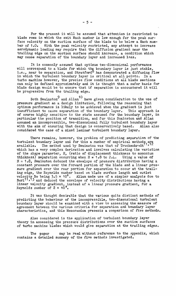
For the present it will be assumed that attention is restrioted to blade rows in which the exit Mach number is low enough for the peak surface velocity on the suction surface of the blade to be below a Mach number of 1.0. With the peak velocity restricted, any attempt to increase aerodynamic loading may require that the diffusion gradient near the trailing edge on the suction surface should increase, a condition which may cause separation of the boundary layer and increased loss.

It is commonly assumed that optimum two-dimensional performance will correspond to a blade for which th boundary layer is just stable, lee., near to separation, 8 and Stratford has demonstrated a diffusing flow in which the turbulent boundary layer is critical at all points, In a turbo machine however, the precise flow conditions at all blade sections can only be defined approximately and it is thought that a safer basis for blade design would be to ensure that if separation is encountered it will be progressive from the trailing edge,

Both Swainstong and Allan 10 have given consideration to the use of pressure gradient as a design limitation, following the reasoning that optimum performance is likely to be achieved when the gradient is just insufficient to cause separation of the boundary layer. This approach is of course highly sensitive to the state assumed for the boundary layer, in particular the position of transition, and for this Swainston and Allan assumed an incompressible, two-dimensional fully turbulent boundary layer with the aim of ensuring that design is conservatively based. Allan also considered the case of a mixed laminar turbulent boundary layer.

There remains, however, the problem of predicting separation of the turbulent boundary layer and for this a number of empirical methodT,aJiS available. The method used by Swainston was that of Truckenbrodt 9 which has a very complex derivation and involves calculating the variation of the shape parameter, H, (ratio of displacement thickness to momentum thickness) separation occurring when H = 1.8 to 2.4. Using a value of H= 1.8, Swainston deduced the envelope of pressure distribution having a constant pressure over the forward portion of the blade and a linear pres- aure gradient over the rear portion for separation to occur at the trailing edge, the Reynolds number based on blade surface length and outlet velocity Be being 3.5 x IO'. Allan made use of a simpler analysis due to Burii1,13 and deduced the envelope of velocity distributions having a linear velocity gradient, instead of a linear pressure gradient, for a Reynolds number of 2 x IO'.

It was thought desirable that the various quite distinct methods of predicting the behaviour of the incompressible, two-dimensional turbulent boundary layer should be examined with a view to assessing the measure of agreement between the various criteria for separation and boundary layer characteristics, and this Memorandum presents a comparison of five methods.

Also considered is the application of turbulent boundary layer theory in assessing the pressure distributions over the auction surfaces of turbo machine blades which would give separation at the trailing edges,

The paper may be read without reference to the Appendix, which contains a detailed summary of the five methods investigated.

-6-

2.70 Flow models

The flow within a turbo machine is complex in nature and at the present time the characteristics of the precise nature of the flow over the surfaces of the blades is a matter for speculation, However, to provide a common basis for analysis three f1ov.r models, whosesurface velocity distributions could be considered to give a simplified representation of distributions associated with the suction surfaces of turbo machine blades, were selected. The models are sho<Jn diagrammatically in Figure 1.

2.1 Surface velocity distributions

To compute th, 0 incompressible boundary layer characteristics and position of separation the velocit,y distribution at the outer edge of the boundary layer is required, Therefore, simple velocity distributions, in the sense that the computations were made easier as vii11 become evident on reading Section 3,0, nere chosen.

The distributions are shown non-dimensiona1l-y in Figure l(a) as velocity ratio V plotted against distance x where V is the ratio of velocity-at outer edge of boundary layer to the velocity at the trailing edge and x is the ratio of surface distance, measured from the leading edge stagnation point, to total surface length. For all three distributions it was assumed that the velocity rose from zero at the leading edge stagnation point to a definite value over an infinitely small distance. The distributions are referred to as type A, B and C,

Tme A - the velocity decreases linearly with surface length from V = V, at the leading edge to V = 1.0 at the trailing edge.

Q-peB- the velocity is constant, v = To, over the first 60 per cent of the blade surface followed by a linear decrease to trailing edge.

TQpe C - the velocity increases_linearly over the first 60 per-cent of blade surface from V = 0.5 at the leading edge to V =

TO at the 60 per cent station, follolfed by a linear decrease to the trailing edge.,

2.2 State of boundary layer

In order to _oredict the behaviour of the turbulent boundary layer the position of transition must be known.

The flow in the boundary layer as it develops from the leading edge stagnation point is initially laminar. The laminar boundary layer is very sensitive to disturbances in the presence of a positive pressure gradient iOeo, pressure increases in the direction of flo;i, and will readily separate or become turbulent,

It is frequently assumed that design will be conservatively based if the boundary layer is taken as being fully turbulent (momentum thickness zero at leading edge). However, J, H. Prestonlb has shown that for a circular pipe and a flat plate the minimum ;ieynolds number, based on momentum thickness 8, for turbulent flow is Ito = 320 and suggests that in the case of flow with a favourable pressure gradient the minimum value will decrease and for flow v:ith an adverse gradient trill increase.

-7-

In view of this it was assumed in the present analysis that the boundary layer was fully turbulent, having a momentum Reynolds number Be of 500 (Figure l(b)) at the leading edge, This approach although not strictly correct should help to ensure that design is conservatively based, since a laminar boundary layer grows at a slower rate than a turbulent layer, Thus, if in practice a length of laminar layer occurs and is followed by transition to iurbulent flow, it is believed that the momentum thickness at the position of,the start of the turbulent layer would be less than if the flow had been fully turbulent.

‘2-o 3 Reynolds number

The present methods of analysis for the turbulent boundary layer are based on data from experiments conducted at Reynolds numbers which were very much higher than is associated with the flow within a turbo machine. In the present study it eras assumed that these methods could be applied to flows where the Reynolds number, Be, is low and representative of turbo machines0 The Revnolds number, based on outlet velocity and blade surface length, range" 2 x IO5 to 1 x 10 , the aim not only on the position of betcfeen the various methods

examined for all three flow models was Re = being to assess the effect of Reynolds number separation but also the measure of agreement of analysis, . I

3.0 Methods of analysis ---_..__- --_

There are in existence several semi-empirical methods of predicting the characteristics of the incowp~ossible, tt-Jolcij.,e,ls.i.onal turbulent boundary and the methods considered TJere thos Truokenbrodt"j12, Stratford'7, Maskell 18

due to B~rill9~3, . and Spencelpj

3.1 Buri

For floby along a flat plate in the a3sence of a pressure gradient the 1/7th po;Jer law for the velocity profile in a turbulent boundary layer may be considered an approximate empirical relation, To specify the velocity profile in the presence of.a pressure gradient Buri chose, in analogy to IL Pohlhausen's approximate method for laminar boundary layers,

a form parameter I? = $ I&j 4 dV dx and assumed that the shearing stress at the

wall a, and the shape parameter H are functions of I' alone.

Thus, =w 7

Q" = .fi(F) .

andH = displacement thickness 6" momentum thickness =-F = f2 03

Experimental data were used to cotiirm the analogy, and the results were moderately satisfactory.

The position of separation involves the calculation of I' over the surface and using the momentum integral equation Buri was able to shorn that

$ (BR&) = A-E .

-8-

where A and B are empirical constants. . .

A unique critical value of I' is then assigned to the point of separation ijhich corresponds to the condition of local skin friction

=w , coefficient Cf = +- = 0.

2pva According to the curve Buri drew through the

experimental points the value of i'critical is -0.06.

The main advantage of this method is that it is fairly straight- forward to compute and does not involve further arbitrary assumptions regarding the value of the shape parameter at transition which can grossly affect the conclusions in some other methods. However, this method involves a knowledge of the velocity gradient, g, which may prove to be difficult to assess from measured pressure distributions.

Both the empirical relationship and rcritical were derived from very limited early experiments of Nikaradse and Burl *II J3, *The experiments of Nikaradse nere for flow in converging and diverging channels having flat walls and of rectangular cross section. Buri's experiments were for flow in converging channels and of circular cross section. In the case with an adverse pressure gradient (divergent channel) the boundary layer was very thick and extended as far as the centre of the channel, the Reynolds number based on momentum thickness Q ranging from 3000 to 9000, For the flow with a constant and favourable pressure gradient (convergent) the range of Be was 500 to 3000,,

Hovrarth'lC has applied Buri's criterion using a value of I'critical = -O,O6, to a measured pressure distribution over a circular cylinder at a Reynolds number based on diameter of 2.12 x IO'. In vien of the assumptions in the calculation (i.e., position of transition, conditions at transition), and the experimental difficulty in locating the separation point the result may be considered satisfactory,

It is north mentioning here that Howell 15 has made use of Buri's parameter in analysing compressor cascade resultso By assuming the velocity distribution in the boundary layer on a cascade blade is linear at separation Hovel1 found fairly good correlation between diffuser and cascade test results.

It was found necessary, in the present analysis, to adopt a more conservative value of rcritiOal for types A and C flow models than had been suggested previously in order to yield results which compare favour- ably with predictions by more recent methods. The validity of such procedure is obviously open to suspicion. On the other hand, the original experiments defining rcritical (with adverse pressure gradient) involved boundary layers extending as far as the centre of the channel, This could have produced secondary flows and thus destroyed the two-dimensionality of the flow assumed in von K.&&n's classical derivation of the momentum equation rihich in conjunction with the measured velocity profiles, Buri used to calculate the tirall shear stress 71;50

302 Truckenbrodt

This method has a very much more complex derivation than that proposed by Buri,

-9-

Location of the position of separation involves the calculation of momentum thickness 8 and shape parameter HO Unlike the other investi-. gators who used the momentum integral equation for 8, Truckenbrodt used the energy integral equation, For calculating H both the momentum and energy integral equations were used0

. The calculation hinges upon semi-empirical relationships between

W energy dissipation in the boundary layer D and Reynolds number based on momentum thickness X0

D 0.56 x 10'~

pv"= -se"

(ii) wall, shear stress l;w, shape parameter H and Rs

TW Cf =

0,246 -= +.M 0.676H 00266

IO %

(iii) a unique relationship between H and a parameter z

if=, 1.269H _ o,g7g ; where H = energy thickness -7 momentum thickness

The momentum thickness is given by

$ (BR;) = A - EX'

where I' eR: dV = - - and the constants Aand B depend on the empirical V dx . .

relationship for the energy dissipation, In arriving at this equa,tion it was assumed that the shape parameter has little effect on the growth of the momentum thickness and was taken as being constant and equal to 1 .I+.

Using the above relationships and the momentum and energy integral equations it can be shown that

- 10 -

Truckenbrodt succeeded in transforming this equation by introducing a shape factor L, which is related to the shape parameter H (see notation), so that it could be integrated and thus obtained an equation for the variation of shape parameter0

The final separation criterion is to ascribe a critical value to He Unfortunately this is not known with any certainty but difficulty can be avoided by calculating the variation of local skin friction coefficient Cf and applying the condition Cf = (Section 3.4).

0 at separation as in Maskell's method

The advantages of this method are firstly that the calculation of shape parameter H is not grossly affected by the value of H at transition and secondly that no derivatives of the velocity distribution with respect to distance along surface are needed, in contrast to the Buri, Maskell and Stratford methods, The calculation, however, is long and laborious when carried out by hand using an electrical desk machine, particularly if com- mencing from a measured pressure distribution,

The equation for the energy dissipation (Rotta) has a very complex derivation; for details see References 12 and 20,

The relationship for the shear stress 7;vf was obtained by Ludweig and Tillmana for flow under the influence of both adverse and favourable pressure gradients by means of a simple instrument developed by Ludweig2Z0 This instrument enables the wall shearing stress to be determined by a heat transfer measurement, The experimental apparatus consisted of a channel of rectangular cross section, one c~all being used as the flat test plate on which the boundary layer measurements were performed, and the other wall adjustable to give the desired pressure distribution. The instrument was calibrated by setting the apparatus for flow with uniform static pressure, the calibration sheering stress being determined by the Schultz-Grunon friction law for plate flow

%f = 334 (log:o;)1.83e

This law, nhich is in close agreement with others for plate flow, was chosen because it was obtained from measurements in the same experimental configuration, Four different test series were carried out, constant pressure, moderate pressure rise, strong pressure rise and pressure drop, the range of Reynolds number RC being IO' to 4 x IO'. The formula was also checked for disturbance in the boundary layer by carrying out two tests at constant pressurez-

(i> with a turbulence grid consisting of metal strips upstream of the measuring section to increase the free stream turbulence

(ii) with a continuous square section strip placed just downstream of the leading edge of the test plate, crosswise to the direction of flow.

The relationship between H and ?i was determined by Weighardt23 from A

the velocity profile law the numerical constants being

- 11 -

adjusted to give agreement with experiment, These experiments were for flow with constant, favourable and adverse pressure rises at high values of Re and the experimental configuration eras similar to that of Lud1iei.g and Tillman, *

There appears to be only one independent experimental pressure distribution to which this method has been applied, this being for the flow over the suction surface of an N.A.C.A. isolated aerofoil'1~12~~ on which separation of the turbulent boundary layer occurred0 The test was carried out in a low turbulence two-dimensional wind tunnel, the pressure . distribution being similar in shape to type A flow model of the present analysis, at a Reynolds number based on the blade chord of 2.64 x ?C? o The agreement between the experimental and calculated boundary layer momentum thickness and shape parameter was very good, separation occurring when H = 2,2,

3.3 Stratford

Stratford's criterion for separation of the turbulent boundary layer results from an approximate solution to the equations of motion and requires a single empirical factor0

The method assumes that the boundary layer in a pressure rise may be divided into two distinct regions, namely the inner and outer regions0

In the inner region, the inertia forces are small so that the velocity profile is distorted by the pressure gradient until the latter is largely balanced by the transverse gradient of' shear stress.

In the outer region the pressure rise just causes a lowering of the dynamic head.profile, and the losses due to the shear stress are almost the same as for the flow along a flat plate*

. A parameter B is incorporated in the first term of a series expan- sion representing the whole inner layer profile obtained by mixing length theory, with the higher terms omitted; B is assumed to represent the effect-on.the.separation criteria of the higher terms, It is also used to represent any effects which the pressure rise might have on the mixing length. -

The final-equation contains a parameter In' which is the flat plate comparison profile at the position of separation, the relevant Reynolds number R, being that based on the peak velocity and the distance to the point of separation. Klebanoff26 8

Stratford found using the data of Schubauer and a d the results of his ovm experiment with'continuously zero

skin friction that n = logiORs but suggests that the criterion is not sensitive to the value of n,

The criterion, which is obtained as a simple formula applying directly to the separation point, was developed for pressure distributions in which a sharp pressure rise starts abruptly after constant pressure for a distance xoo The distance x is measured from a pseudo origin which is the point where the turbulent boundary layer would have zero thickness,

After simplification the criterion, order of 106,

at a Reynolds number of the is given by a simple formula

- 12 -

where

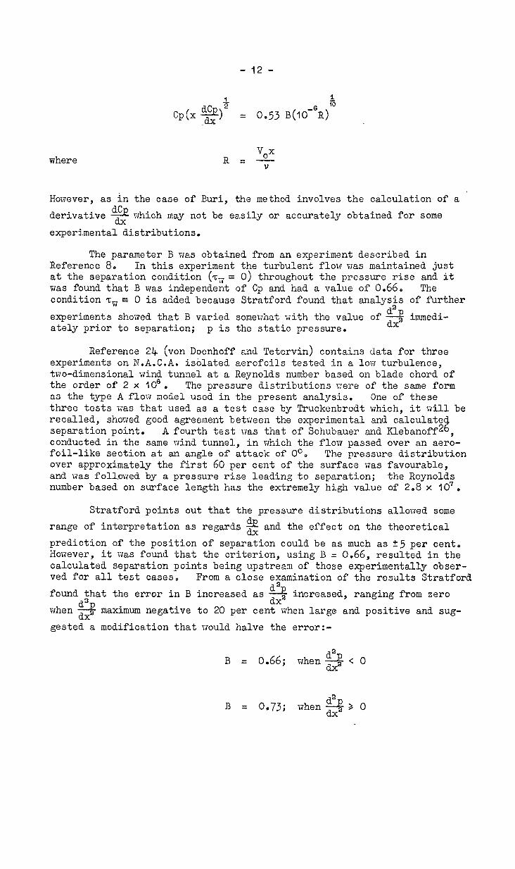
However, as in the case of Buri, the method involves the calculation of a derivative $$ - which may not be easily or accurately obtained for some experimental distributions.

The parameter B was obtained from an experiment described in Reference 8. In this experiment the turbulent flow was maintained just at the separation condition (71J = 0) throughout the pressure rise and it was found that B was independent of Cp and had a value of 0.66, Tie condition r~\~ = 0 is added because Stratford found that analysis of further experiments shoned that B varied somewhat with the value of dap immediately prior to separation; p is the static pressure. dxa

Reference 24 (von Doenhoff and Tetervin) contains data for three experiments on E.A.C.A. isolated aerofoils tested in a low turbulence, two-dimensional wind tunnel at a Reynolds number based on blade chord of the order of 2 x IO6 m The pressure distributions Rere of the same form as the type A flon model used in the present analysis. One of these three tests was that used as a test case by Truckenbrodt which, it will be recalled, showed good agreement between the experimental and calculate separation point. A fourth test was that of Schubauer and Klebanoff2 % , conducted in the same sirind tunnel, in which the flow passed over an aerofoil-like section at an angle of attack of O". The pressure distribution over approximately the first 60 per cent of the surface was favourable, and was followed by a pressure rise leading to separation; the Reynolds number based on surface length has the extremely high value of 2.8 x IO'.

Stratford points out that the pressure distributions allowed some range of interpretation as regards 9

dx and the effect on the theoretical prediction of the position of separation could be as much as 25 per cent, However, it vas found that the criterion, using B = 0.66, resulted in the calculated separation points being upstream of those experimentally observed for all test cases0 From a close examination of the results Stratford found that the error in B increased as dap

d3 dX2 increased, ranging from zero

when -d$ maximum negative to 20 per cent when large and positive and suggested a modification that would halve the error:-

B = 0.66; when $$ < 0

2 B = 0*73; rrhen$-$) 0

- 13 -

The advantage of Stratford's method is that it is extremely simple to apply since it does not involve graphical integration as do the other methods or a step-by-step solution for the shape parameter as does Maskell's method. In fact it was found, using an electrical desk machine that whereas the methods of Maskell, Truckenbrodt and Spence took the author at least half a day to apply and Buri about one hour, Stratford's method took only half an hour. This, of course, does not apply necessarily to all types of flovi since for the models used in the present analysis the boundary layer was assumed to be turbulent over the entire sur-

faoe, Horrever. the method demands the calculation of a derivative which may not be easily obtained for some experimental pressure

distributions. Also if one is interested in other boundary layer characteristics, such as local skin friction coefficient, then an alter- native method would have to be used.

It was found that of the methods considered in this Memorandum Stratford's criterion predicted the lamest pressure rise to separation;

dCp- dx was known exactly in the present analysis, A possible reason for this

is that the factor B was determined from test distributions at Reynolds number Be ranging from 2 x IO6 to 2 x IO7 whereas for the flow models the Reynolds number was very much loner and it may be that B varies somewhat when Be < IO'.

3.4 Maskell

Maskell's method is based upon a large amount of experimental data not only for flat plate and channel flow but also for flow over isolated aerofoils.

The position of separation involves the calculation of the momentum thickness and shape parameter, the equations for which have been made more general than before by making them fit flat plate data very closely and by the use of some limited data for favourable pressure gradients*

The equation for the momentum thickness was derived from the momentum integral equation, in a manner similar to that of Buri, making use of the Ludweig and Tillman relationship for skin friction:-

& (6R;) = A - BI'

eRi dV where I' = - - Vdx

and A, B and n are empirical constants, n being determined to make the solution correct for zero pressure gradient,

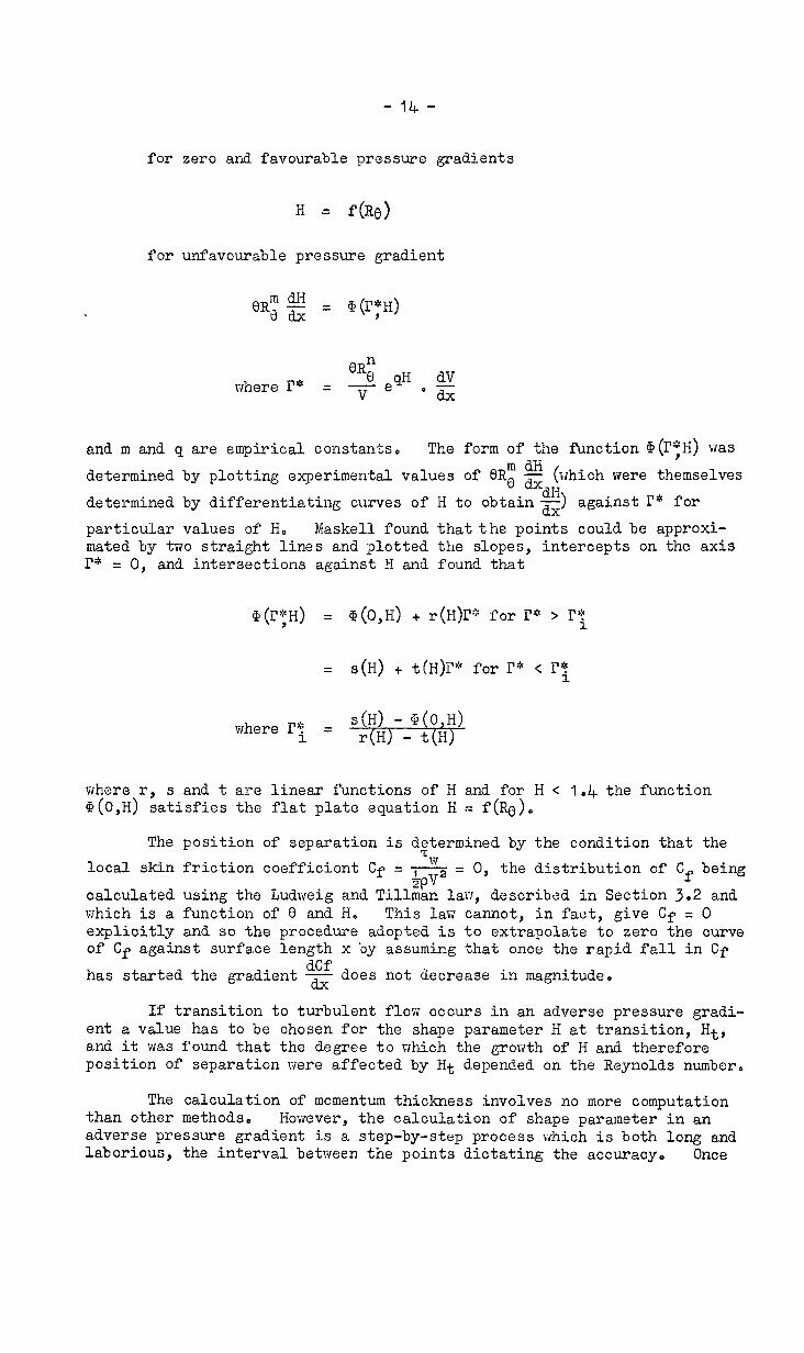
The approach used to find an equation for the shape parameter H was that of selecting the probable parameters affecting the variation of H, and using experimental data to find an equation connecting them, This approach, which has been used by other investigators24, was well suited to the nature of the available data. The form of the equation is:

- 14 -

for zero and favourable pressure gradients

Ht f(%)

for unfavourable pressure gradient

mdH eRa dx = %(I';H)

eR: qH where I'* = - e dV V o- dx

and m and q are empirical constants, The form of the function G(I':H) was determined by plotting experimental values of BBC m g (which dx were themselves

determined by differentiating curves of H to obtain dx against i'" for dK)

particular values of H. Maskell found that the points could be approxi- mated by two straight lines and plotted the slopes, intercepts on the axis I'* = 0, and intersections against H and found that

G.(F;H) = @(O,H) + r(H)l?* for I'* > I';

= s(H) + t(H)I'" for I'* < rf

where r, s and t are linear functions of H and for H < 1.4 the function Q(O,H) satisfies the flat plate equation H = f(RC)O

The position of separation is dttermined by the condition that the local skin friction coefficient Cf = Z

+pTra = 0, the distribution of Cf being

calculated using the Ludweig and Tillman lava, described in Section 3.2 and which is a function of 0 and H, This law cannot, in fact, give Cf = 0 explicitly and so the procedure adopted is to extrapolate to zero the curve of Cf against surface length x by assuming that once the rapid fall in Cf

has started the gradient dCf dx does not decrease in magnitude.

If transition to turbulent flow occurs in an adverse pressure gradient a value has to be chosen for the shape parameter H at transition, Ht, and it was found that the degree to which the growth of H and therefore position of separation were affected by Ht depended on the Reynolds number.

The calculation of momentum thickness involves no more computation than other methods. However, the calculation of shape parameter in an adverse pressure gradient is a step-by-step process which is both long and laborious, the interval between the points dictating the accuracy0 Once

- 15 -

again the method depends on the calculation of a velocity gradient, and when experimentally determined pressure distributions are employed it becomes susceptible to the same sources of error as the methods of Buri and Stratford,

The empirical relationships for momentum thickness and shape parameter were derived from experiments conducted at a Reynolds number of the order 2 x IO'. Four of these experiments were in fact used by Stratford and one by Truckenbrodt as test cases.

Unfortunately all of the available experimental data was used in deriving the empirical relations 30 that no independent comparisons with experiment are presented, However, the comparisons with the data show that the boundary layer characteristics and position of separation can be predicted with reasonable accuracy for practical purposes,

The result of applying this criterion to the flow models of the present analysis was that the pressure rise to separation was much higher than that according to Stratford's criterion. This was surprising in view of the number of common test cases for which these two methods have been demonstrated to be in agreement with experiment. However, it must be remembered that the velocity distributions for all of these cases were similar to those of the type A flow model only, except one which was similar to that of type C, and 'the Reynolds numbers were very much higher than the range considered in the present study.

3.5 Spence

This method involves the calculation of the momentum thickness 0 and shape parameter H,

The equation for momentum thickness was derived from the momentum integral equation aa in the methods of Buri and iViaskel1, the difference in the solution being the assumption of the 1/5th power law for the skin friction coefficient,

In determining an equation for the variation of shape parameter, Spence made use of the momentum and energy equations aa did Truckenbrodt, Using theseequations it can be shown that

ndH eRe dx = Q(H)I' - e(H)

ORi dV .where I' = - - - vdx

In arriving at this expression assumptions were made regarding

(0 distribution of shear stress within the boundary layer

(ii) velocity profile in a variable pressure

(iii) wall skin friction coefficient,

- 16 -

The above equation is of the same form as that used by Truckenbrodt and Maskell, the solution of which varies in the choice made for functions Q(H) and $(H). Spence chose relationships such that the equation could be integrated directly and so avoided the calculation, as did Truckenbrodt,

dV of the velocity gradient duo a To ensure that good results are given for a flat plate with zero

pressure gradient, i,e., I = 0, the function q(H) was determined from the momentum equation assuming

(i> one-fifth power law for the wall skin friction coefficient c f

= 0.0176 1

Re" (ii) Cole's relationship for the shape parameter

uT where E; = - f: v log, RC + constant

C2? C I, are constants/and U, is the friction velocity.

For the function G(H) a quadratic was chosen.

For the case of a thick boundary layer and using a value of Ho = Id+ where V = V,, Spence shows this to be in good agreement with the functions used by Maskell.

The final separation criterion is to ascribe a critical value to H, which as Spence points out, is not known with any certainty. To overcome this the position of separation can be determined by the condition Cf = 0, the distribution of Cf being again calculated using the Ludneig and Tillman law.

There appears to be only one case for which this method has been demonstrated to be in agreement with e over an isolated aerofoil-like section* "s

eriment and that is for the flow

10'. at a Reynolds number of 2.8 x

It is in fact one of the distributions that was used by Stratford and Maskell as a test case0 The pressure distribution was favourable over the first 60 per cent of the surface followed by an adverse pressure' rise leading to separation, transition to turbulent flow occurring near the leading edge. The comparison between the calculated and experimental distributions of momentum thickness and shape parameter was good, separation occurring when H = 2.6. In the calculation of H a value of lo4 was assumed at the position of the peak velocity.

The advantage of this method over those of Maskell and Truckenbrodt, which also involve the calculation of H, is that the distribution of H over the surface is more rapidly calculated. Another advantage over Maskell's method, which is however shared by Truckenbrodt's method, is that the solution does not involve the calculation of the first derivative of velocity

dV with respect to surface distance -0 dx The result of applying this method to the flon models was that the

velocity gradient to separation was grossly affected by the value assumed for H at transition whereas Truckenbrodt's method is not; a change from I,3 to 1.4 grossly affects the conclusionso Also the growth of shape parameter was very little affected by a change in Reynolds number, Re

- 17 -

* . resulting in the pressure rise to separation other methods-showing that en increase in.Re .

4.0 Results of comparison 1 -:.

1 1 '4.1 * A 'Momentum thickness, l

being constant with Re,.the ‘delays separation.

,I *

,: .* -All of the'methods.e&cept Stratford's,involve the calculation.of

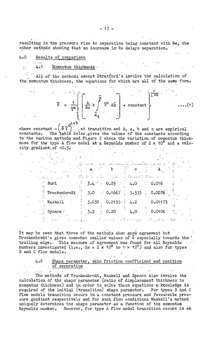
the:Lmomontum thickness, the equations for which 'are all of the same form. . 1 . .I ,: I . . . . . ’ 8:

.* .J” . ,- ._

k +6-- ,a

g = 1

I

Tc d'; Ta: ikb

s

? * . - 1 ‘.

+ constant .,,.(I)

Xt- a) 1

l+b e'v

a where constant =

t j at transition and A, a, b and c are empirical

constantp. The...abl below.gives the values of the constants a&cording. to the various.methods and Figure 2 show the variation-of momentum thickness for the type A flow model at a Reynolds number of 2 x, 105, and a velocity gradient.,of. --Oe5; _ a . - .

; .'I *- - I . . . - ._ 1. 1. . .

. . .. ' . 6 ' :.. ..A ,.. ..I . " ;. . . ,.,.. ,. . . ,' :.. . " : " ,...- "_ : -.. . . ".. -. _ - .;; . I 1 . a : .

.,, ._. b p1 c ; . A*‘. ’ ; .. : .d .

II. ..v 1,* . .: ./ . . : *. -. . . “. .. I... . : : . . . . . . . . . . . ” . . . . . ,

;: -Buri . ii 3a4 a': 0.25 . ’ 4.0’ i 0.016 i, .

'I Truckenbrodt i 3.0 .’ 0.1667' ; 3@333 i 0.0076~ ‘il. :: . ,:* . : .’ .

’ _ " Maskell L 0.2155-i 4.2 - 0.01173 . ’ ’ r . i . ; 3.632:

.i

.'- Spence.! I

. 11 j 3.5 _I 0.20 i Lt.0 ; 0.0106 I;.. . . -

_/ -.’ . . . . ,T.. . .’ . . . . . . ‘; . . . ~. . . . . ..I. ..: ..” :‘..., I . I .

It may be seen that three of the methods show good agreement but Ir ' Truckenbrodt's gives somewhat smaller values of 0' especially towards the ' trailing edge.. This measure .of agreement was found for all Reynolds . . . numbers investigated (i,e,,.Re = 2 x IO' to 1,x lO?).and also for types B and C flow models. ‘

402 . t . .

Shape'parameter,' skin friction coefficient and position . of separation I. , .

. . . , 6. . . . The meihods.of. Truckenbrodt, Maskell and Spence also involve the

calculation of the shape parameter (ratio of displacement thic‘kness to momentum thickness) and in.order to solve these equations,a:knoxledge is required of the initials (transition) shape parameter. .For types B and C f1a-J models transition occurs.in a constant pressure and favourable pressure gradient respectively and for such flow conditions Maskell's method uniquely determines the shape parameter as a function of the momentum Reynolds number. However, for type A flow model transition occurs in an

- 18 -

adverse pressure gradient and so a value for the transition shape parameter, Ht, has to be assumed in this method. To solve the equations of Truckenbrodt and Spence a value for Ht has to be assumed for all flow conditions.

The local coefficient of skin friction is particularly important for two reasons. Firstly it is a measure of the velocity gradient at the surface and therefore, the stability of the boundary layer, and secondly to investigate blade temperature distributions which may be required in the stress analysis of turbine blades the distribution of heat transfer coefficient is required which, using Reynolds analogy, is related to the skin friction coefficient. According to Ludweig and Tillman the skin friction coefficient is given by

z Cf .= ,T--$ = 0.246 e

40581H -o*aaa % . ..*(2)

On examining this equation it may be seen that if the initial value of H affects the distribution of shape parameter it will also influence the local value of Cf and hence the position of separation (given by Cf = 0) and local heat transfer coefficient. In view of this results are presented (Figures 3 to 9) showing the distributions of shape parameter and skin friction coefficient for a range of Ht = 2 x IO' and I x IO'.

I,3 to 1.7 at Reynolds number of It is seen that the velocity gradient is varied as

well as the Reynolds number and the reason for this is that it is considered desirable to assess the effect of Ht on the position of separation, Therefore, the gradients were selected such that separation occurs at the trailing edge for Ht = 1.4 which is the commonly assumed value.

Figures 3, 4 and 5 show the distributions according to Truckenbrodt's method of analysis for types A, B and C flow models respectively. The shape parameter (and therefore the displacement thickness) and skin friction coefficient are not grossly affected by the value of Ht, only in a region close to the transition point are the differences in H and Cf significant, particularly when transition occurs in constant pressure or pressure rise regions at low Reynolds number.

The characteristics H and Cf using Spence's method are shown in Figures 5, 7 and 8. It was found that the calculation of H was very little affected by a change in Reynolds number or in ether words to a change in the distribution of momentum thickness and so the shape parameter is shown for the low Reynolds number only, For types A and B flow models, Figures 6 and 7 respectively, the distribution of H and Cf are grossly affected by the value of Ht in particular the range of 1.3 to 1*4, over the entire surface for both Reynolds number. In applying this method to type C model, Figure 8, it was found that the shape parameter dropped off rapidly to a value of approximately 1.2 at the start of the pressure rise and thereafter remained approximately constant, This resulted in very high values for Cf and thus indicated no separation point. By assuming a value for H of 1.4 at the start of the pressure and continuing the computation of H in the normal way beyond this point the method predicted separation. However, as in the case of A and B flow models the pressure rise to separation is especially sensitive to the initial value of H.

- 19 -

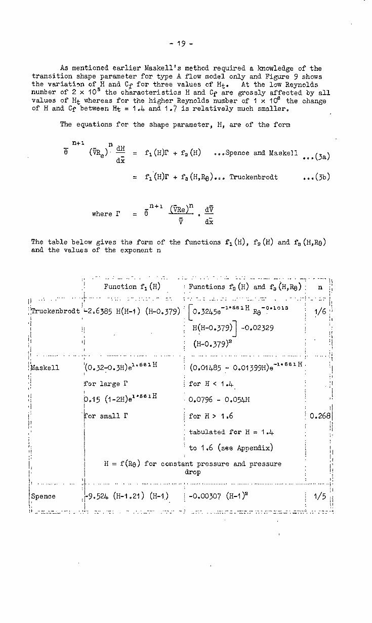
As mentioned earlier Maskell's method required a knowledge of the transition shape parameter for type A flow model only and Figure 9 shows the variation of H and Cf for three values of Ht. At the low Reynolds number of 2 x IO5 the characteristics H and Cf are grossly affected by all values of Ht whereas for the higher Reynolds number of I x IO' the change of H and Cf between Ht = I.4 and I.7 is relatively much smaller,

The equations for the shape parameter, H, are of the form

= fl (H)r + fi (H) . ..Spence and &IaEkell .0.(3a)

= fl‘(H)p + f,(H,Ro).,. Buckenbrodt . ..(3b)

where I' = 8 n+l (TRe)n o a

7 a;;

The table below gives the form of the functions f,(H), f,(H) and fc(H,B) and the values of the exponent n

:, . .I’ .” . .._ ., -. . . ::. ” : _. :I . . ,. I .:. :. -‘: . . . . . I. ..-. .._.. . ._ - _“ ” . . “.“.I

: Function f,(H) : Functions f2(H) and fc (H,Q) : . n :i !, ..: . ;.-' . . , . . . .,, . " ; . . . i . . . :."'.:'.:.", .- ..". Y".' "..E ..I.. .:'.: . ..." ':...'.'L- - . .. L-p :..' Ii

i$ruckenbrodt'L2.6383 H(H-1) (H-0,379)' 0.32.!+5e-10661H Q-o*"" i

; l/G ;i . Ii :I I ! !i ; H(H-0.379) -0.02329 ; !

; (H-O.379)2 1

;/ f;

!: ii

ii . .

il

I, ~;

.I / ii

j. . . . . . . . . . . . . . . ,J. . .

i, ..*.... . . . . . . . . . . . . . . . . , . . . . . . . . . . . . . . . . . . . . . . . . . . . . . , . . . . . . . . . ,. . . . . . ..;

!i$askell 3'

i: :(0.32;0.3H)e1'"81H i (0.01485 .- 0001399H)e-1'661H~ '1

:i jI

:I for large i? i for H < 1.4 2. ; 1 !

11 8. If

p.15 (1-2’H)e1*681H : 0,07Y6 - 00054H ‘1 I

i! 'bar small p i for H > 1.6 ii

i 0.268i I! f I:

I tabulated for H = 1.4 ;j :i :.

' to 1.6 (see Appendix) I !i

i' 1

i ‘ i ! H

= f(Re) for constant pressure and pressure : II jI

drop i: . . . ..,, . . . . . . ;I. . . . .,,. . . . . . .

i . . . . . . . . . . . . . . . . ;. . . . . . . .,...........,. . . . . . . . . . . . . . . . . . . . . . . . . . . . . . . . . . . .i . . . . . . . . . . ..j!

ISpence I1

,19.524 (H-l 21) (H-I.) ; -0eOO307 (H-1)' ; l/5 j; I. i ir

- 20 -

It is worth mentioning here that Truckenbrodt was able to integrate the above equation for H by introducing a shape factor, which is related to the shape passeter (see Appendix), and thus avoided the calculation of

the derivative 2 o Spence also integrated the differential equation for

H,

In the present study the integrated equations were used. Figure 10 shows a plot of the above functions for a range of H = 1.3 to 1.7. The value of Truckenbrodt's function fo(H,Re), is shovdn for Ro = 1509 500 and 6000 these values being found in the present study for the type C model just downstream of transition, at the leading edge for all three flow modals and the maximum value respectively0 It is to be noted that in Uaskell' s method the above equation fcr H only holds for flow with pressure rise. For the other flow conditions, i.e., constant pressure and pressure drop, the shape parameter is a function of the momentum Reynolds number.

Considering Spence's function f,(H) it ma.y be seen that its value is very small and negative and remains approximately constant with H. The reason for this is that Spence made use of the one-fifth power late for skin friction to deduce the form of f,(H) and this law shows that the skin friction is independent of H, Therefore, as a first approximation, Spence's equation shows that for flow with pressure rise and pressure drop H is given by the first term of Equation (ja).

The value of f,(H) changes rapidly with H and as a result the calculation of H was grossly affected by the initial value of shape paremeter (Ht) for the above flow conditions, Also on examining the above approximate equation it may be seen that for a given velocity distribution the calculation of H is not affected by a change in Reynolds number, Re, as was found in the present study.

The value of Naskell's function f,(H) and Truckenbrodt's function f,(H,Re) varies rapidly with H and as a result the distribution of H is sensitive to a change in Reynolds number as will be seen later. Truckenbrodt's function varies from positive when H < 1.4 to negative and large when H = 1.7 resulting in the distribution of H not being grossly affected by a change in the value of Ht' Kaskell's function for large l? is small, negative and approximately constant and equal to the value of Spence's when H < 1 o4 and for H > 1.4 drops off rapidly to large and negative values when H = 1.70 Therefore, it is to be expected that the calculation of H for cases where I? is large will be particularly sensitive to values of Ht in the range 1.3 to 1.4. However, for small r the function varies rapidly for all values of H and so it is not obvious that the growth of H will be independent of the initial value for this case0

As mentioned earlier Spence's method when applied to type C flea model did not predict a rapid rise in the region of pressure rise. For this model the first term of Equation (3a) was large and negative over the first part of the surface due to the velocity, V, being small and a positive velocity gradient in this region, Therefore, H dropped rapidly to a value of approximately 1.2 at the start of the pressure rise (x = 0.6) and

-.21 -

for this value of H the function f,(H) is very small resulting in a constant value for H of approximately 1.2 in the region of pressure rise, However, Truckenbrodt's method also showed a drop in H to 1.2 just downstream of the transition point at the low Reynolds number but downstream of this region the calculation showed a rise in H to 1.4 at the start of pressure rise and in the region of pressure rise H rose rapidly (Figure 5). The reason for this was that in the region where H = 102, the momentum Reynolds number was small (Re = 150) resulting in the second term (Equation 3b) being sufficiently large and positive in comparison to the first term for the calculation to give positive rise in the shape parameter*

2 and, consequently, a

In the case of constant pressure H is given by, according to the methods of Spence and Truckenbrodt

..'.(5b)

It is easily seen from the plot of f,(H) and fc(H,&)'why the former of these methods is very sensitive to the value of Ht for such flow conditions and the latter approximately independent of Ht.

It is not cbvioua from plct of the functions f,(H), fs (H) and fc(H,Q) that the above three methods will be in agreement regarding the calculation of H for any particular value of Ht. The generally accepted value for the transition shape parameter for flow at high Reynolds number is I *4, which is the flat plate or constant pressure value for H, although there is experimental evidence24 that Ht can be as high as 1.8 in SOme

* cases. A comparison of the distributions of H and Cf using the methods of Truckenbrodt, Maskell and Spence, is shown in Figures II, 12 and 13 fcr types A, B and C flow models respectively at a Reynolds number, Re, of 2 x IO' and 106 and a value of 1.4 for HtO The velocity gradient S is -0.5, -0.75 and -I,0 for A, B and C models respectively.

Truckenbrodt's criterion for separation is that the shape parameter H, takes the value of 1.8 to 2.4 and it may be seen that this results in a wide range for the position of separation, Maskell's criterion is that the skin friction coefficient, Cf, is zero at separation and in view of the good measure of agreement Maskell foun?, between experimental and theoretical positions of separation it was decided to adopt this criterion for comparing the above three methods.

Considering type A flow model, Figure II, it may be seen that at Re = 2 x IO' the methods of Truckenbrodt and Spence are in reasonable agreement regarding H but Maskell's deviates greatly from these methods giving very much lower values over the last 40 per cent of the surface, As regards the distribution of Cf significant differences occur over-the last part of the surface and the position of separation varies from x = O,& according to Spence to L = 1.0 according to Maskell. However, at

- 22 -

the Reynolds number of -lethe methods of Maskell and Truckenbrodt are in good agreement but Spence deviates greatly from these methods, predicting the same values for H as at the lower Reynolds number for the reason mentioned earlier.

Turning to type B flow model, Figure 12, at the high Reynolds number all three methods are in tolerable agreement regarding both H and Cf but at the lower Reynolds number whereas Maskell and Spence are in good agreement Truckenbrodt shows very much higher values of H and consequently lower values for Cf in the region of pressure rise,

For type C model, Figure 13, all three methods are in tolerable agreement in the region of

P ressure rise,

pressure drop (2 However, in the region of

= 0 to 0~6 there are significant differences in the distribution of H and Cf at Re = 2 x 105. Truckenbrodt's method shows very low values of H in this region compared to Maskeli's and the reason for this is that the value of Truckenbrodt's function fs(H,Re) is strongly dependent on the momentum Reynolds number, Re, which drops rapidly from 500 at the leading edge to 150 at Z = 0.2.

Various methods for relating blade shape to surface velocity distribution are clprently being examined and the question arises as to what is the optimum velocity gradient which should be aimed at in design. Figure 14 shows, for the flow models considered in this study, the variation of adverse velocity gradient, p with Reynolds number, Re, for separation at the trailing edge (j; = l.Oj using, the criterion Cf = 0 and a value of Ht = I ,4, in the above three methods. Also shown are the gradients using the separation criterion of Buri and Stratford, Buri's cri-

terion for separation is that a parameter I' eR@s dv

= - - = -0.06 at separa- V dx tion but in view of the limited experimental data from which this value was derived the velocity gradients were also calculated for I' = -0-04.

Stratford's criterion predicted the lowest pressure rise to separation for all flow models except type A at high Reynolds number. However, it must be pointed out that the pressure rise to separation according to Stratford is likely to be from 0 to 10 per cent too low since asp is small and negative, dxa

Spence's method showed that the critical velocity gradient was independent of Reynolds number and had the same value for types B and C flow models for the reasons mentioned earlier. However, the other methodc of analysis showed that the effect of increasing Reynolds number is'to delay separation,

4.3 Application to turbomachinery design

The Mach number over the suction surface of a blade may be as high as unity and so the applicatio of incompressible boundary layer theory is questionable. Van Driest11t2g has shown that for flat plate flow i.e., zero pressure gradient, the effect of Mach number on the local coefficient of skin friction is small up to M = 1.0 and can be neglected, the ratio 'fM= 1 - being O,Y3, but there appears to be no evidence available for flow C fM= 0 under the influence of pressure rise.

- 23 -

Without reliable experimental measurements of the boundary layer development and separation relating to flows typical of those within turbo machinery it is not possible to comment confidently on the particular validity of any of the methods considered in this Memorandum in such an appli- cations In a typical turbo machine both Reynolds number and turbulence differ substantially from those appertaining to experimental data on which each of the five methods has been based, and against which each has been tested in varying degree,,

Under these circumstances preference leans naturally to the use, as a guide, of the method which is simplest to compute or which yields the most conservative solution, particularly in the lower range of Reynolds number. Stratford's method would seem to combine both these attributes commendably, so far as provision of a convenient criterion for separation is concerned.

However, if the boundary layer characteristics such as displacement thickness and skin friction coefficient are required then it is suggested that 'Pruckenbrodt's method be used since it does not involve the calculation of local velocity gradients g as does Maskell's and is not so sensitive to the shape parameter at transition as the methods of Maskell and Spence.

From the results shown in Figure 14 it was considered possible to construct two envelopes of velocity distributions for separation at the trailing edge

(a> distributions of type B having a constant velocity over the forward portion of the blade followed by a linear decrease to trailing edge and,

(b) distributions of type C having a favourable velocity gradient over the forward portion followed by a linear decrease to the trailing edge, ~

Figures 15 and 16 show the critical envelopes for types B and C according to Stratford's criterion and it is suggested that until definite eqeri- mental data become available for the flow conditions over the surfaces of turbo machine blades the envelopes for a Reynolds number of 2 x IO" should be used as a limiting criterion in design.

500 Conclusions

Five methods of predicting the behaviour of the incompressible, two-dimensional turbulent boundary layer have been applied to three basic types of velocity distribution, selected to represent the family of distributions associated with turbo machine blades, and the measure of agreement between the separation criteria and boundary layer characteristics assessed, The methods considered were those due to Buri, Truckenbrodt, Stratford, Maskell and Spence,

The velocity distributions that were analysed were type A - linear decrease of velocity from leading t\> trailing edges of the blade, type B - constant velocity over the first 60 per cent of the blade surface followed by a linear decrease to the trailing edge and type C - linear increase of velocity over the first 60 per cent of the surface followed by a linear decrease to trailing edge.

- 24 -

The precise flow conditions over the surfaces of a blade in a turbo machine is a matter for speculation, but for the present study it was assumed that the boundary layer flow was fully turbulent with a momentum Reynolds number of RC = 500 at the leading edge.

The methods of Truckenbrodt, Maskell and Spence provide the growth of the shape parameter and to solve these equations an assumption has to be made with regard to the transition (i,eo, initial) value Hte Spence's method was extremely sensitive to the value of HtO Sven a small change from I,3 to 1.4 grossly affects the distribution of H and, therefore, the position of separation, Truckenbrodt's method was very little affected by Hte Maskell's method only reqtiires the initial value of H when transition occurs in an adverse pressure gradient and it was found that the extent to which the growth of H and pressure rise to separation were affected by Ht depended on the Reynolds number.

The equations for the momentum thickness were of the same form and all of the methods were in good agreement except Truckenbrodt which showed smaller values.

Spenoe's method showed that the pressure rise to separation was independent of Reynolds number whereas the other methods showed that the effect of increasing Reynolds number is to delay separation.

All the methods could be brought into tolerable agreement regarding the position of separation provided that

(0 (ii)

(iii)

(iv>

Buri's criterion was taken as I'critical = -0.04.

In applying Spence's metho,d the calculaticn of shape parameter started at the position of maximum velocity, if transition occurred upstream of this point.

For the methods of Truckenbrodt and Spence the Ludweig and Tillman law was used to calculate the variation of local skin friction coefficient Cf and the position of separation was given by the condition Cf = 0 and not by a predetermined value of shape parameter H. Since this law cannot yield explicitly Cf = 0, the point of separation was obtained by linear extrapolation from the steepest negative gradient of the Cf curve0

For the methods of Truckenbrodt, Maskell and Spence the variation of shape parameter was calculated using an initial value of H = 1.4e

On reviewing the methods, al.1 of nhich derive from experimental conditions somewhat removed from the environment within a turbo machine, Stratford's was simplest to apply, predicted the lowest pressure rise to separation, and is therefore preferred as a conservative design criterion.,

On this basis envelopes of critical suction surface velocity distributions (i,e., distributions which yield trailing edge) were constructed which,

separation conditions at the it is believed, are conservatively

based and might be used as a limiting criterion for turbo machine blade design,

- 25 -

If the boundary layer characteristics such as displacement thickness and skin friction coefficient are required then it is suggested that the method of Truckenbrodt be used as it does not involve the calculation of local velocity gradients 2 and is not grossly affected by the value of the Shape parameter at transition.

No, Author(s)

1 0. Zweifel

2 D. G. Ainley G, C. B. Mathieson

3 A, R, Howell

4 J, D. Stanitz

5 J. D. Stanitz L, J, Sheldrake

6 Chung-Hua Wu

7 E. Martensen

8 B, S. Stratford

9 M. J. C. Swainston

IO W. K. Allan

- 26 -

REFERENCES

Title, eto,

The spacing of turbo machine blading especially with large angular deflection, The Brown Boveri Review Vol, 32, No. 12 1945

A method of performance estimation for axial-flow turbines. R, & M. 2974, December, 1951

Fluid dynamics of axial compressors, Design of axial compressorse The Institution of Mechanical Engineers, Proceedings Vol. 153, 1945 pp. 441-462

Design of two-dimensional channels with prescribed velocity distributions along the channel walls* N.A.C.A. Report 1115, 1953

Application of a channel design method to high-solidity cascades and tests of an impulse cascade with 90' of turning. N.A.C.A, Report 1116, 1953

A general theory of three-dimensional flow in subsonic and supersonic turbo machines of axial - radial and mixed - flow types, N.A.C,A. TN.2604, January, 1952

Berechnung der Druckverteilung an gitterprofilen in ebener potentialstro- mung mit einer Fredholmschen Integral- gleichung, Archive for rational mechanics and analysis. Vol. 3, No. 3, 1959

An experimental flow with zero skin friction throughout its region of pressure rise. Journal of Fluid Mechanics Vol, 5, Part I, PP.1 7-35, 1959

The boundary layer characteristics of some hypothetical turbo machine blade pressure distributions, Ae9.C. 23,568, February, 1962

Theoretical analysis of the performance of cascade blades, A.R.C. 23,061 July, 1961

- 27 -

l3FERENCES (cont'd) --

J&*

11

Author(d

H. Schlichting ,

12 E. Truckenbrodt

Title, etc.

Boundary layer theory. McGraw-Hill Book Co. Inc., New York, 555-590, 1960

Ein Quadraturver fshren zur Berechnung der laminaren und turbulenten Reibung- sschicht bei ebener und Rotationssymmet- nischer Stromung. Ingenieur - Archiv 20, 211-228 .I952

13 A.Buri _ A method of calculation for the turbulent (translated from the boundary leyer with accelerated and

'German by M. Flint) retarded basic flow. R.T.P. Trans. No. 2073. Issued by the Ministry of Aircraft Production

14 L. Howarth

15 A. R. Howell

16 J. H. Preston

17 B. S. Stratford

18 E. C. Maskell

19

20

21

B. Thwaites

J. Rotta

H. Ludweig I?. Tillman

Note on the flow past a cirouler cylinder, Proceedings of the Cambridge Philosophical Society Vol. 5, Port 4, 1935

The present basis of axial flow compressor design. Part I - Cascade theory and performance. R. 6'. Ma 2095, June, 1942

The minimum Reynolds number for a turbulent boundary layer end the selection of a transition device. Journal of Fluid Mechanics, Vol. 3, part4, 1958 PP~ 373384

The prediction of separation of the turbulent boundary layer. Journal of Fluid Mech,anics, Vol. 5, Part I, 1959 PP.I-16

Approximate calculation of the turbulent boundary layer in two-dimensional incompressible flow. A.R,C.l4 654, November, 1951

Incompressible Aerodynamics. Oxford at the Clarendon Press, 1960

Schubspannungsverteilung und Energie- dissipation bei turblenten Grenzchichten. Ingenieur-Archiv 20, 195-207, I952

Investigation of the wall shearing stresses in turbulent boundary layers. N.A.C.A. T.M. 1285, May, 1950

- 28 -

Author(sl Title, etc.

22 H. Ludweig An instrument for measuring the skin . (translated by friction coefficient of turbulent boundary

Sylvia We Skan the Aerodynamics Division, N,P.L.)

layers. B.R,C.12 991,

23 IC. Wieghardt VI. Tillmen

On turbulence pressure, N.A.C.iL T.M.

24 E. A. von Doenhoff Determination N. Tetervin the behaviour

layers. --

March, 1950

friction layer for rising

1314, October, 1951

of general relations for of turbulent boundary

I"r.R.C. 6845, F.M. 597 and N.A.C.A. R772, ~qx-il , 1943

25 G. B. Schubauer P. S. Klebanoff

26 ~ E. R, Van Driest

Investigation of separation of the turbulent boundary layer. N e A. C.A. TN,21 33, August, 1950

Turbulent boundary layer in compressible fluids. Journal Aero. Sci., Vol. 18, No. 3, March, 1951 pp.l45-I 60

- 29 -

NOTATION

D

H

ii

L

M

Re

Re

R

U

energy which is converted into heat in the laminar boundary layer

boundary layer shape parameter displacement thickness = momentum thickness

parameter = energy thickness momentum thickness which is related to H

parameter which is related to H by

L = s &r where gp I* 1.73

Mach number

Reynolds number based on velocity at outer edge of boundary layer and momentum thickness

V0 =- v

Reynolds number based on velocity at trailing edge and blade surface length

v2e =-

V

Reynolds number based on maximum surface velocity and surface distanoe

velocity within the boundary layer

I

z UT . friction velocity = JZ

\ p

V velocity at outer edge of boundaxy layer

ii ratio of velocity at outer edge of boundary layer to velocity at . trailing edge

ji. an equivalent distance defined by Equation (21)

K ratio of distance measured along blade surface (from leading edge stagnation point) to'total blade surface length

CP incompressible pressure coefficient = 1 -($ k 1 -g-j

T Cf local coefficient of skin friction = 2X-

&pv2

e

P

t ,

X

Y

P

6

8

e'

s*

tP*

P

V

%W

I?

r*

ri

blade surface length

- 30 -

static pressure

energy of the turbu+ent motion per unit time for a turbulent boundary layer

distance measured along surface of blade from leading edge stagnation point

distance normal to surface of blade

velocity gradient = -

boundary layer thickness

momentum thickness of boundary layer

ratio of momentum thicla?ess to blade surface length

displacement thickness .of boundary layer

energy thickness of boundary layer

density

kinematic viscosity

shearing stresses at the blade surface

parameter = V 8 dx S kn dV

parameter = ii e 0 mH kn dV 8 z

parameter defined by Equation (36~) in Appendix

Subscripts

t conditions at the transition point

0 maximum conditions and position of maximum conditions

a conditions at the trailing edge of the blade

- 31 -

APPENDIX1

The prediction of the characteristics of the turbulent boundary layer

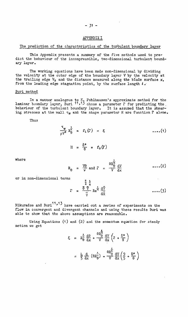
This Appendix presents a summary of the five methods used to predict the behaviour of the incompressible, two-dimensional turbulent boundary layer.

The working equations have been made non-dimensional by dividing the velocity at the outer edge of the boundary layer V by the velocity at the trailing edge V a and the distance measured along the blade surface x, from the leading edge stagnation point, by the surface length e.-

Buri method

In a manner analogous to K, Pohlhausen's approximate method for the laminar boundary layer, Buri i1913 chose a parameter I' for predicting the. behaviour of the turbulent boundary layer. It is assumed that the shearing stresses at the wall 7;w and the shape parameter H are function p alone.

Thus

where

or in non-dimensional

1

RO = %i dV F and I' = -- Vdx

.0..(l)

. ...(2)

terms 5 1 5; - -

r = r d? Bv Be4 d;; v

Nikuradse and Buri II,13 have carried out a series of experiments on the flow in convergent and divergent channels and using these results Buri was able to show that the above assumptions are reasonable.

Using Equations (I) and (2) and the momentum equation for steady motion we get

- 32 -

hence

-& (eR$ = o...(4)

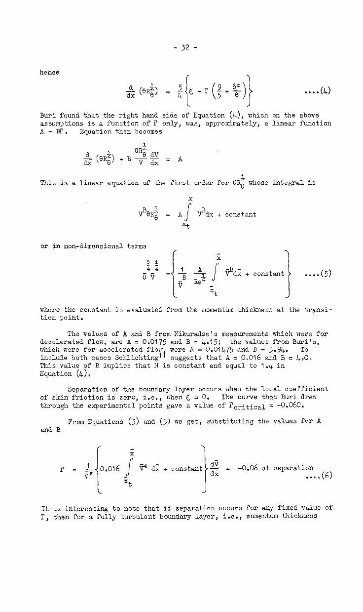
Buri found that the right hand side of Equation (4), which on the above assum:3tions is a function of T only, was, approximately, a linear function A - BI'. Equation then becomes

$ ('3Ri) + B eR; dv -- = A V dx

This is a linear equation of the first order for BR: whose integral is

V'%R~ = A[ VBdx + constant

Xt

or in non-dimensional terms

s 1 zs

ev I 1 = --ii ii A

Rez 2 t

. ..0(5>

where the constant is evaluated from the momentum thickness at the transition point,

The values of A and B from Nikuradse's measurements which were for decelerated flow, are A = 0,0175 and B = 4.15; the values from Buri's, which were for accelerated flop: were A = Oe01475 and B = 3.940 TO include both cases Schlichting 11 suggests that A = 0.016 and B = 4.0. This value of B implies that H is constant and equal to lo4 in Equation (4).

Separation of the boundary layer occurs when the local coefficient of skin friction is zero, ioeo, when S = 0. The curve that Buri drew through the experimental points gave a value of I'critical = -0.060,

From Equations (3) and (5) we get, substituting the values for A and B

r = dv z

= -0006 at

It is interesting to note that if separation occurs for any fixed value of 1 -', then for a fully turbulent boundary layer, i.e,, momentum thickness

- 33 -

8 =OatG = 0, the condition of separation is independent of Reynolds number Rez if the velocity distribution does not vary with Ree o

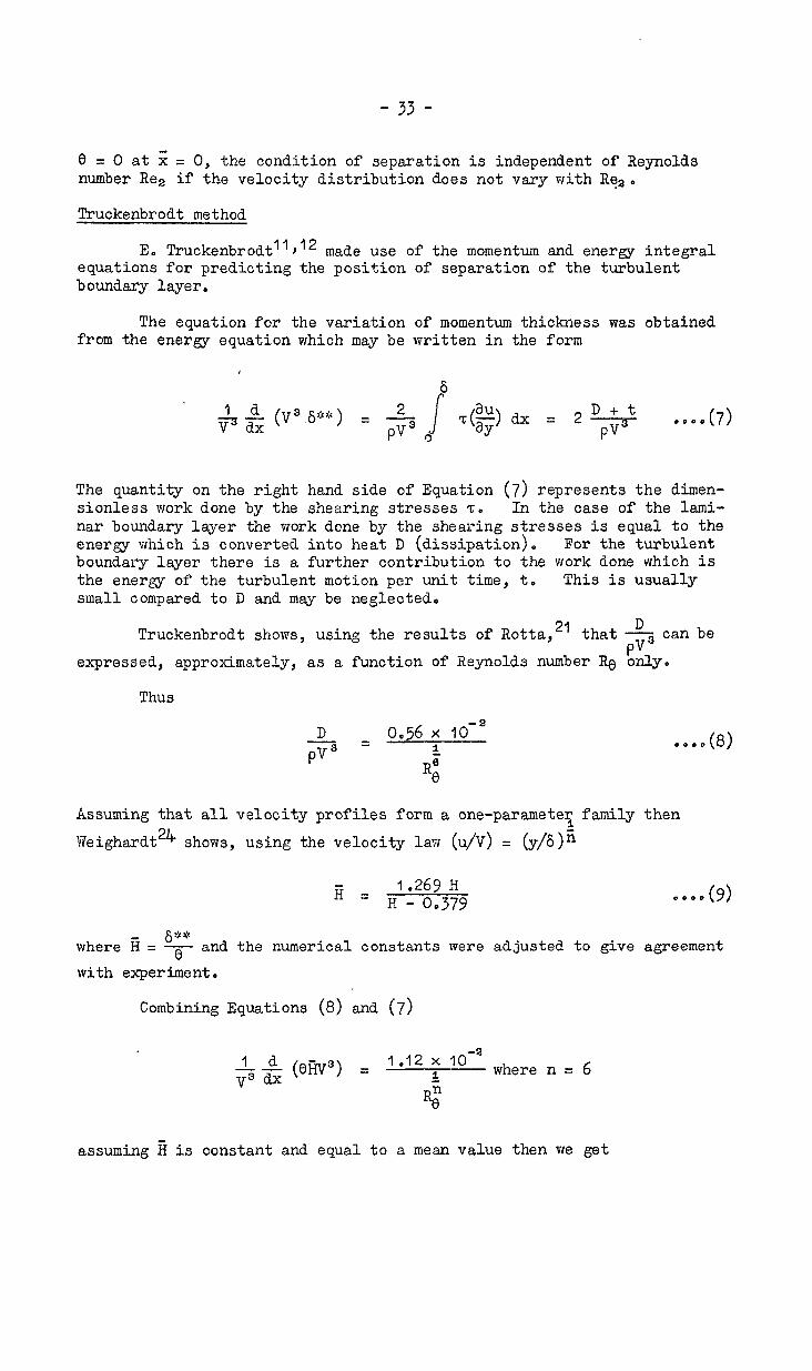
Truckenbrodt method

E. Truckenbrodt11T12 made use of the momentum and energy integral equations for predicting the position of separation of the turbulent boundary layer,

The equation for the variation of momentum thickness was obtained from the energy equation which may be written in the form

Id 72.2

6

I=-$ i T'$dx = 2D+t --r

*o..(7) d

The quantity on the right hand side of Equation (7) represents the dimen- sionless work done by the shearing stresses 'G. In the caze of the laminar boundary layer the work done by the shearing stresses is equal to the energy which is converted into heat D (dissipation). For the turbulent boundary layer there is a further contribution to the work done which is the energy of the turbulent motion per unit time, t. This is usually small compared to D and may be neglected.

Truckenbrodt shows, using the results of Rotta, 21 that D - can be

expressed, approximately, PV3

as a function of Reynolds number R.c only,

Thus

D 0.56 x 10-a pv3= 1 o...(8)

Ri

Assuming that all velocity profiles form a one-parametex family then Weighardt24 shows, using the velocity law (u/V) = (~/6)~

a = H 1,269 H - 0.379 odY>

where g = !$? and the numerical constants were adjusted to give agreement

with experiment,

Combining Equations (8) and (7)

where n = 6

assuming E is constant and equal to a mean value then we get

- 34 -

or

3. i

ii de eRi dV Rez+3 v dx =

1.12 x lO-a -- ii

1 & $ (*$) + 3 !$ g =

( ). le.12 x 10-a * _

H

or 1.

& (en!) + (3 + %, v-F& = ORi dV 1.12 x 10-a n+l

ii o- n

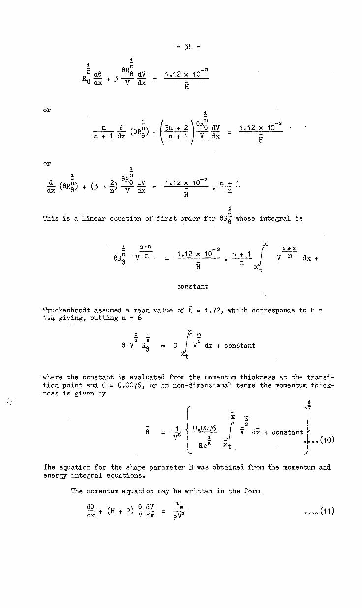
This is a linear equation of first order for 6i$ whose integral is

2 3+3 X

3 ,+ a

OR; .vT. = 1.12 x iO-a n+l o- s

VT dx+ Ti n

Xt

constant

Truckenbrodt assumed a mean value of g = 1.72, which corresponds to H 2 l,L+ giving, putting n = 6

10 i X

6 V3 R; = C ‘2

V3 dx + constant

where the constant is evaluated from the momentum thickness at the transition point and C = 0.0076, or in non-dimensional terms the momentum thickness is given by

6

v dL + I:onstant

The equation for the shape parameter H was obtained from the momentum and energy integral equations.

The momentum equation may be written in the form 7;

g+(H+2)$g = 4 PV

. . . ..(I?)

- 35 -

Replacing 6** in the energy Equation (7) by fi0 and from this equation subtracting Equation (II) multiplied by B we obtain, multiplying through

1 by R;

i - .eRfJ dH

8Z = r#)r + f,(E) .oe.(12)

where

fl(@ = (H - I)& f,(g)

i

eRi dV and I' = vz

The shearing stresses at the wall zw, using the results of Ludweig and Tillman22, can be expressed as a function of Re and H.

Thus z

W

pva=

o.,23 ,0-0.d78H Re-O.=e a-(13)

Truckenbrodt transformed Equation (12) into such a form that it could be integrated, by introducing a shape factor L. This factor is related to the shape parameter H thus

L(B) = s

aFi f,= L(H)

E&l

where the lower limit of integration was chosen to make L = 0 correspond to the case of zero pressure gradient, ioer, flow over a flat plate, giving Hp = 1.73 and H = 1.4.

Introducing this relationship into Equation (12) we get

1: ORe dL edx = r - K(L)

where i<(L) = f2 03 -- =

flm K(g)

The function K(L) can be represented with a satisfactory degree of accuracy by the linear relation

. . ..(14)

K(L) = a(L - b) .,..(15)

- 36 -

The numerical values are

a = 0.0304 and b = 0,07 log,,Ro - 0.23

Combining Equations (14) and (15) we obtain a linear differential equation for L which Truckenbrodt integrated giving

where 000076

b = 0.07 loglo (Re 7 e') - O,23

and

It is to be noted that the new variable S occurs in the equation for momentum thichess (10).

According to work of Ludweig and Tillman the shear stress at the wall IYW decreases as the shape parameter increases but never vanishes com- pletely. Truckenbrodt assumes that separation occurs Flhen H = 1.8 to 2.4 which corresponds to L = -0,13 to -O,l8,

Stratford method

The separation criterion due to Stratford'7 results from an approximate solution to the equations of motion, The method assumes that the turbulent boundary layer in a pressure rise may be divided into two distinct regions, namely the inner and outer regions.

In the inner region, the inertia forces are small so that the velocity profile is distorted by the pressure gradient until the latter is largely balanced by the transverse gradient of shear stress.

In the outer region the pressure rise just causes a lowering of the dynamic head profile, and the losses due to the shear stresses are almost the same as for the flow along a flat plate.

The criterion is developed initially for pressure distributions in vJhich a sharp pressure rise starts abruptly at the position x = x0 after constant pressure for a distance xoo

- 37 -

A parameter B is incorporated in the first term of a series expan- sion representing the lyhole inner layer profile, obtained by mixing length theory, and the higher terms omitted; the factor B was assumed to represent the effect on the separation criterion of the higher terms, It is also used to represent any effects which the pressure rise might have on the mixing length, The velocity profile has therefore been over idealized as regards to shape and good agreement with experimental profiles would not be expected,

The oriterion for separation is, applying directly to the separation point

cpJh- a) ( X dCp Yi dx ) =

I 3' x 0.41 B (n - 2 )&(n-a) R6 7 1

(n + l)z(n+L) (n + 2)1 . . ..(17)

n+2 For Cp < n

where the Reynolds number X is bas'ed on the local value of distance x and the peak velocity V,. n+2 The limitation Cp Q n+l results from the join of the inner layer with the outer layer reaching the edge of the boundary layer when using the idealized velocity profiles.

Stratford simplifies Equation (17) by replacing the quantity

cn + , j&+1) ln + 2+

cn _ ,)tb-a >

l(n-a) by 10.7 x (2.0)4 when 6 Q n s 8.

which is within 1 per cent of the former quantity

This results in.

1

= le06 B (10-6R)10 . . ..(18)

The quantity 'II' is the flat plate (zero pressure gradient) comparison profile at the point x = xs where suffix a denotes separation

xa ' the relevant Reynolds number being R, = --$ D Stratford found from

experimental data that a good approximation is

- 38 -

The parameter B was found from an experiment by Stratford, In this experiment the flow was maintained just at the separation condition throughout the pressure rise and it was found that B was independent of Cp and has the value

B = 0.66

However, in this experiment the value of dap dxa

immediately prior to separa-

tion had its greatest possible negative value and B will vary somewhat with

d2p dxa '

To determine the effect of $$ Stratford applied the criterion to four experiments in which separation of the turbulent boundary layer was observed and found that, using a value of B = 0.66, the separation was always too low, A clcse examination of that the discrepancy in B increased with an increase in

0 per cent when da 3 was maximum negative to 20 per cent

large and positive.

pressure rise to the results showed d2p _ varying from dx2 2 when dp was dxa

In view of the insufficient data Stratford suggests that a crude modification that would halve the error would be to take

B = 0.66 when 2 < 0

da B = 0.73 when ---$a 0 1. _

.o..(lY)

Combining Equations (18) and (IY), using a value for n of 6, the criterion for separation is, at Reynolds numbers of the order of IO6

r ?; dCp cp x dx

.( P = 0,3s (IO-* do

or in non-dimensional terms

I 0.39 (10m6 Re ~o~>'o ..0.(20)

when $$ 3 0 and Cp C Lc l

7' the coefficient 0.39 is replaced by 0,35 when

dap (0. dx"

The pressure coefficient for incompressible flow is given by

- 39 -

It will be recalled that this criterion was developed for pressure distributions having an initial region of' constant pressure folloxed by a sharp pressure rise, the distance x being measured from a point where the turbulent boundary layer would have zero momentum thickness.

If transition occurs in the re value of x to be used in Equation

ion of constant pressure then the (20 has to be

2 = (X-q+q 0 0 0 0 (21)

where the distances 2 and j; are the distances from the point of zero momentum thickness (pseudo origin) and the actual leading edge respectively. The value of ?t is determined by the condition that the boundary layer thickness for a fully turbulent boundary layer at &-, is equal to that at Zt for the laminar boundary layer.

where

This results in

Rt =

8, = ,,,.(22)

For pressure distributions having an initial region of favourable pressure gradient the distribution has to be converted to an equivalent one having an initial region of constant pressure with a mainstream velocity equal to the value at the transition point or the point of maximum velocity nhich- ever is later.

The gronth of a turbulent boundary layer is given by, in non- dimensional terms I .-

c St 1 1+b

J 7' dz + constant I

zt

> ..&3)

The parameters a, b etc, according to various workers vary a little but representative values are a = a, I7 b =-r;, c = 4, A = 0.016, The constant

is evaluated from the momentum thickness of the laminar boundary at transition and is given, in non-dimensional terms, by

where

l+b constant C = Pt vtal A % 2

0.470 et = - r r s ii6 Rc o v5 &

w&4)

c-(25)

- 40 -

From Equations (2.2)) (23)) (24) and (25) we get .

. . ..(26)

where suffix-o now refers to conditions at the position of peak velocity or at transition whichever is later and from (21)

x = (ii - X0) + I, . . ..(27)

Equation (26) can be re-arranged to give

This equation differs from Stratford's slightly in which the exponents 4 and -6 are 3 and $ respectively. The reason for this is that.the parameters m, n etc. in Equation (23) have been chosen as the mean values according to various workers, which Stratford agrees is a better approximation.

Maskell method

Maskell' 8 made use of the Lud\;eig-Tillman skin friction law for predicting the position of separation of the turbulent boundary layer. This involves calculating the distribution of the shape parameter H and the momentum thickness 0, the equations for which have been made more general than before by making them fit flat plate data very closely and'by the use cf some limited data for favourable gradients.

The equation for the variation of momentum thickness \?as derived from the momentum equation, in a manner similar to Buri, and making use rf the Ludweig-Tillman law.

The momentum equation may be written

0 0 0 ‘ (29)

- J+l -

The Ludweig-Tillman law gives

Cf = G(H)Rin . . ..(30)

where G(H) = aemmH

Combining Equations (29) and (30) we get

eR: dV Rtf. g + (H + 2) 7 z = G(H).

Re-arranging ae get

where eRe” dV r = -yf-Y&

Xaskcll found that using experimental data the right hand side of Equation (31) may be represented by a linear function of I', reducing the equation to the form

& @Ii;;) = A - El’ o-(32)

It can be seen that Equations (31) and (32) can only agree exactly for r = 0 ioeo, constant pressure, if 11 is constant in plate flow. Ludweig and Tillman found that the shape parameter H nas a function of Q and so Equation (32) is necessarily in error for constant pressure.

To overcome this Maskell makes the substitution

OR: dV I’ = -I

V dx

into the momentum Equation (29). This results in .

Maskell determined the value of q such that when I' = 0, g = constant and using experimental data found that the right hand side of Equation (33) could be represented by

d@R; > dx = e - fI' where e = 0.01173, f = 4.2

Or 6R: dV -I$ (OR:) + f v z = e v,here q = 0.2155

The value of f Equation (33).

= 4*2 implies that H is constant and equal to 1.635 in

whose integral is This is a linear equation of the first order for eg

fJRz Vf = e Vf dx + constant

In non-dimensional terms, the momentum thickness is given by

r 7 1 -I_ ii I. 2155

e’ = 1 ,45-

I

’ fj402~ + constant 0.01173 0.2155

V Re / zt _

i

. . ..(j4-)

where the constant is evaluated from the momentum thickness of the laminar boundary layer at transition,

The approach used in finding an equation for the shape parameter H was that of selecting the probable parameters affecting the variation of H. Experimental results \iere then used to confirm that this choice of parameters was reasonable and to find an equation connecting them, The main reason for adoptin, v this approach was because the available data was best suited to it.

For constant pressure and favourable pressure gradient, the variation of the shape parameter is given by

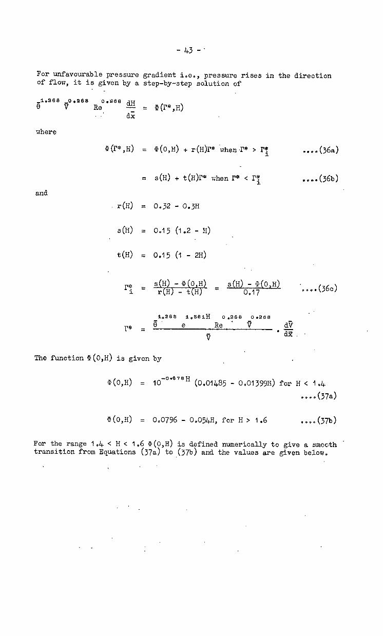
- 4.3 --

For unfavourable pressure gradient iaeo, pressure rises in the direction of flow, it is given by a step-by-step solution of

,ieacia ,ooaes 8 V

0.268 &y Re - . dx:

where

@(r”,H) = O(O,H) + r(H)l?* 'nhen.I'* > P i

and

- r(H) = 0.32 - 0.3H

s(H) = 0915 (1.2 - H)

t(H)

r4 1

= @(l?*,H)

= s(H) + t(H)I'* when I?* c I? 1

= 0.15 (1 - 2H)

...a(36a)

.oc.(36b)

sH - 9(O,H) = s(H) - @(O,H) 8 = r(H) - t(H) 0.17 . . ..(36c)

The function Q(O,H) is given by

Q(O,H) = 10-0'678H (0.01485 - 0,01399H) for H < I.4

..ob(37a)

O(O,H) = 0.0796 - O,O54H, for H > 1.6 ..0*(37b)

For the range 1,4 < H < 1.6 Q(O,H) is defined numerically to give a smooth ' transition from Equations (37a) to (37b) and the values are given below.

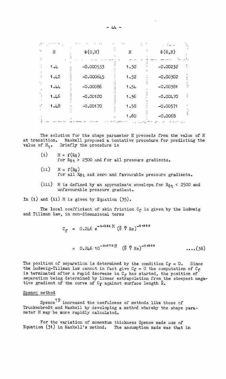
-4-G-

1.4

I 042

~44

1.46

I .l+3

@,H) ’

-0,000533 ;

-0,000645 i

-0.00086 ;

-0.00120 i

-0,00170

H -.

1.50

1.52

1.54

lo56

1.58

1.60 . . .

-0.00232 i

-0~00302 1

-0.00381 ::

-0.00470 j

-0.00571 ’

-0eOO68 i :: ,. ,“. - .,’ .- .-:.- -.

The solution for the shape parameter H proceeds from the value of H at transition, Maskell proposed a tentative procedure for predicting the value of Ht' Briefly the procedure is

(i> H = f(RC) for Ret > 2500 and for all pressure gradients.

(ii) H = f(Q) for all Qt and zero and favourable pressure gradients.

(iii) H is defined by an approximate envelope.for Qt < 2500 and unfavourable pressure gradient.

In (i) and (ii) H is given by Equation (35).

The local coefficient of skin friction Cf is given by the Ludweig and Tillman law, in non-dimensional terms

cf = 0,246 e-105S1H (5 v Re)-ooas8

= 0,246 jO-0’676H (8 v Re)-00a68 ,...(38)

The position of separation is determined by the condition Cf = 0. Since the Ludweig-Tillman law cannot in fact give Cf = 0 the computation of Cf is terminated after a rapid decrease in Cf has started, the position of separation being determined by linear extrapolation from the steepest negative gradient of the curve of Cf against surface length 2.

Spencc method

Spence 19 increased the usefulness of methods like those of Truckenbrodt and Maskell by developing a method whereby the shape parameter H may be more rapidly calculated.

For the variation of momentum thickness Spence made use of Equation (31) in Maskell's method. The assumption made was that in

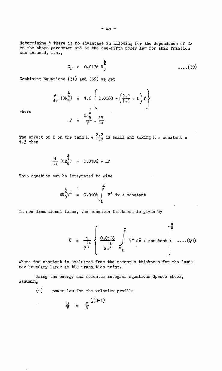
- 45 -

determining 0 there on the shape parame

is no advantage in allowing for the dependence of Cf ter and so the one-fifth power law for skin friction

was assumed, iOeo,

1

Cf = 0.0176 R; .eo.(39>

Combining Equations (31) and (39) we- get

where

2.2 The effect of H on the term H + - , 2 is small and taking H = constant = 1.5 then D

& (OR!) = oeo106 + .!+I'

This equation can be integrated to give

X 1 .

0R;V" = 0.0106 V4 dx + constant

In non-dimensional terms, the momentum thickness is given by

s 2 6

6 = & + constant

I

*...(40> fF-

where the constant is evaluated from the momentum thickness for the laminar boundary layer at the transition point,

Using the energy and momentum integral equations Spence shows, assuming

(i) power law for the velocity profile

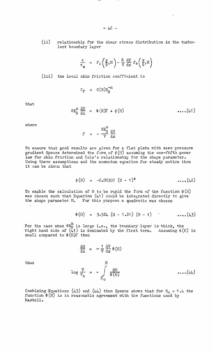
- 46 -

(ii) relationship for the shear stress distribution in the turbulent boundary layer

(iii) the local skin friction coefficient is

Cf = G(H)Rin

that

where 0Ri dV r = ---

V dx

To ensure that good results are given for a gradient Spence determined the form-of $(H)

flat plate with zero pressure assuming the one-fifth power

law for skin friction and Cole's relationship for the shape parameter. Using these assumptions and the momentum equation for steady motion then it can be shown that

t’(H) = -0.00307 (H - I)" . . ..(42)

To enable the calculation of H to be rapid the form of the functipn Q(H) was chosen such that Equation (4.1) could be integrated directly to give the shape parameter H, For this purpose a quadratic was chosen

@CH) = 9.524 (H - 1.21) (H - 1) .' .-(43)

For the case when 0$ is large iaeo, right hand side of (41)

the boundary layer is thick, the is dominated by the first term.

small compared to @(H)I' then Assuming $(H) is

dH dx= -fg@(H)

thus

Combining Equations (43) and (44) then Spence shows that for Ho = ? .4 the function @e(H) is in reasonable agreement with the functions used by Maskell.

- 47 -

Substituting Equations (L&Z) and (43) into Equation (41) and inte- grating we get

X \ Va 4.762 - & constant - 0.00307 q s

i) BR06

where the constant is evaluated from the shape parameter for the turbulent boundary layer at transition,

In non-dimensional terms the shape parameter is given by

Hz I + 40762 - 1 va

.00307

E -6 v -

6 1

-s 0 Re'

where

Spence points out that the value of H at separation seems always to be between 2 and 3 and suggests that the range 2.4 to 2.6 be taken.

D 76913/l/125875 K3 IO/66 R

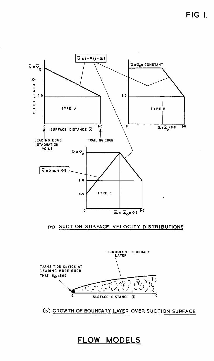
FIG. I.

TYPE A

SURFACE DISTANCE z

t ,iNG EDGE TRAILING EDGE

STAGNATION \

TYPE 0

POINT

(CL) SUCTION SURFACE VELOCITY DISTRIBUTIONS

TURBULENT BOUNDARY LAYER

TRANSITION DEVICE AT LEADING EDGE SUCH \ THAT Ret500

eq

0 SURFACE DISTANCE 5 1-o

(b) GROWTH OF BOUNDARY LAYER OVER SUCTION SURFACE

FLOW MODELS

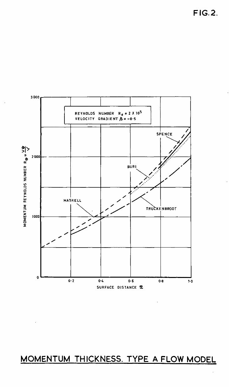
FIG.2.

3000

0

REYNOLDS NUMBER R, = 2 X 10’ VELOCITY GRADIENT p= -0.5

1 /

I 0 MASKELL /

r/ 0 0

/ -( /

/ 0

/ 0 /

o-2 04

SURFACE

00 6 04 100

DISTANCE %

MOMENTUM THICKNESS. TYPE A FLOW MODEL

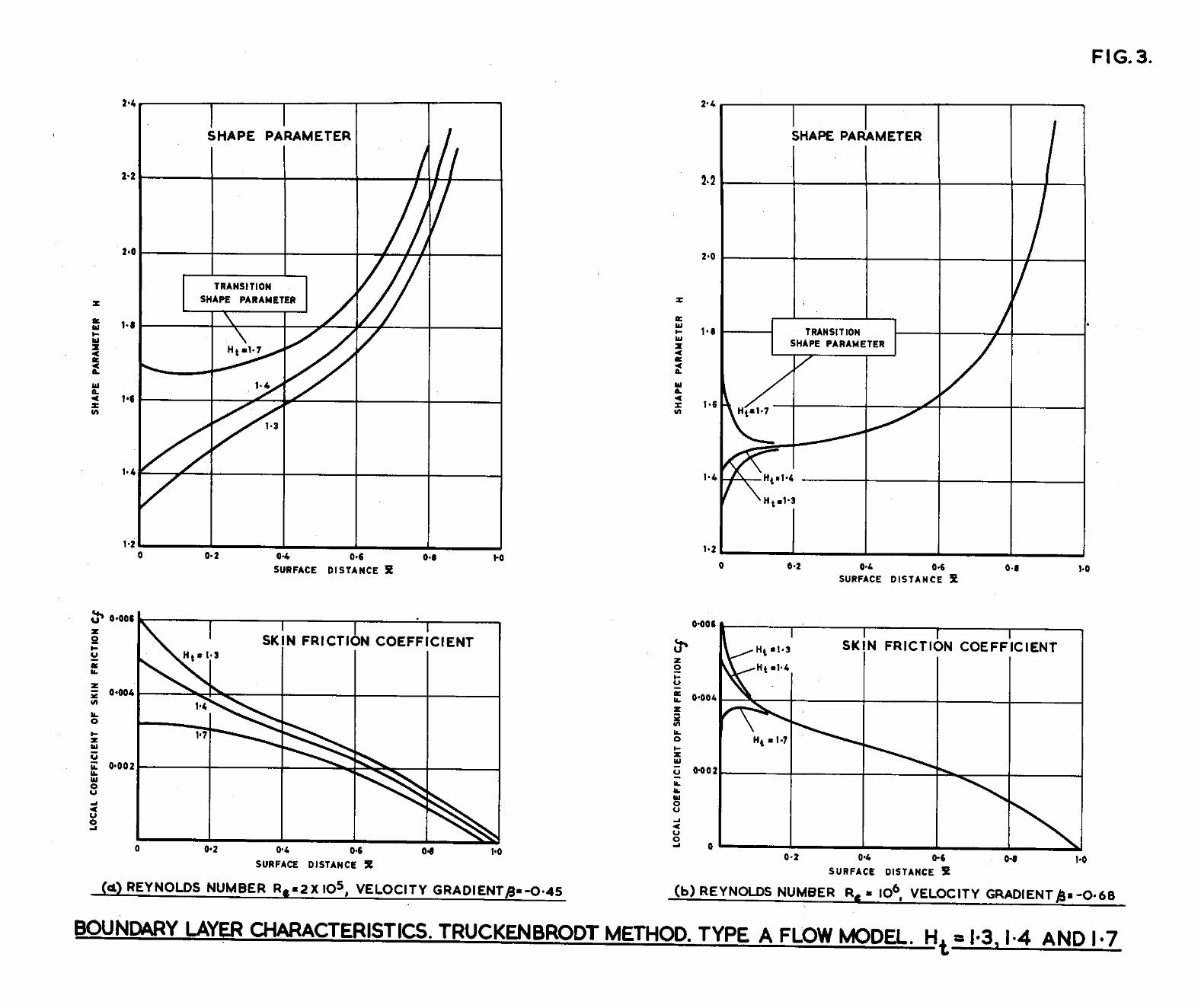
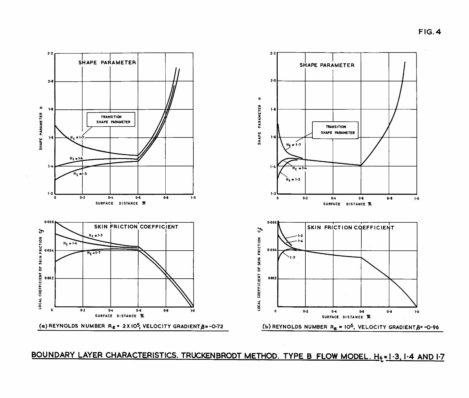
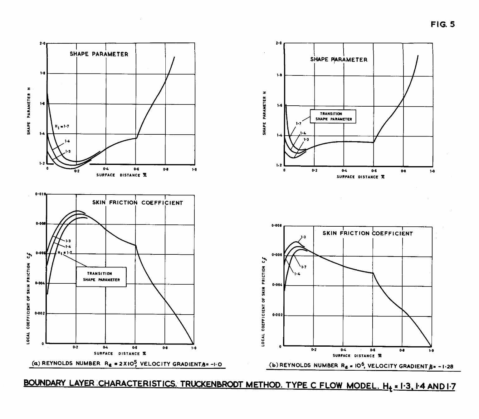
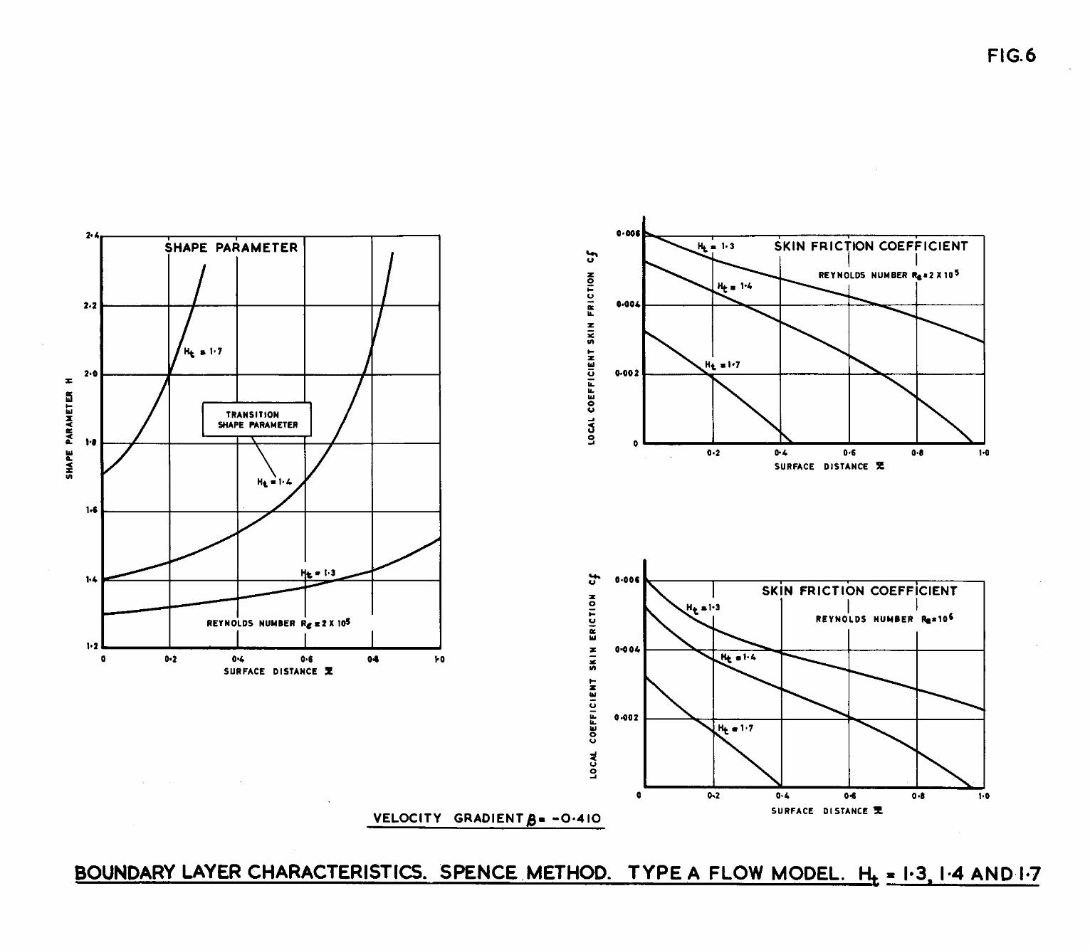
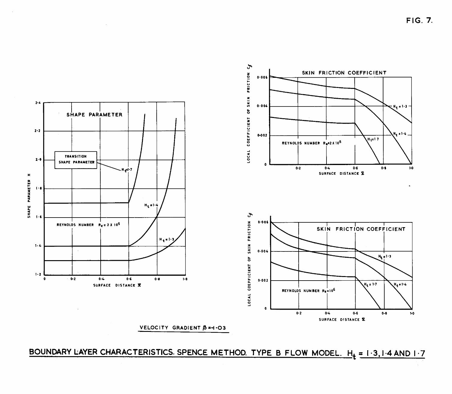
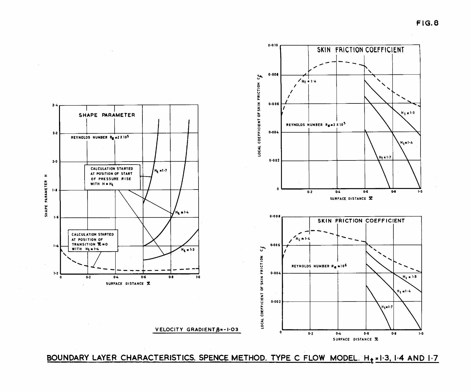
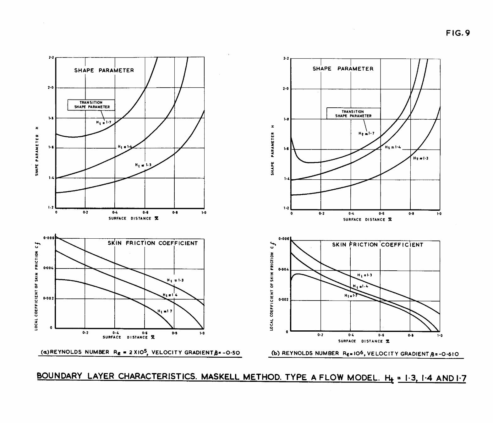
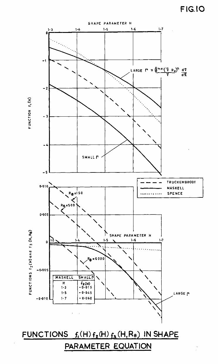
FIG.10

SHAPE PARAMETER H

-1

-1

O’OO!

0

t

LL

-O*Ol(

t. \

\ \

t,

- - - I TRUCKENBRODT

MASKELL I.,-. . . . . . . . SPENCE

LARGE 7

FUNCTIONS f,(W) f,0=0 f&-I,Re) IN %WE

PARAMETER EQUATION

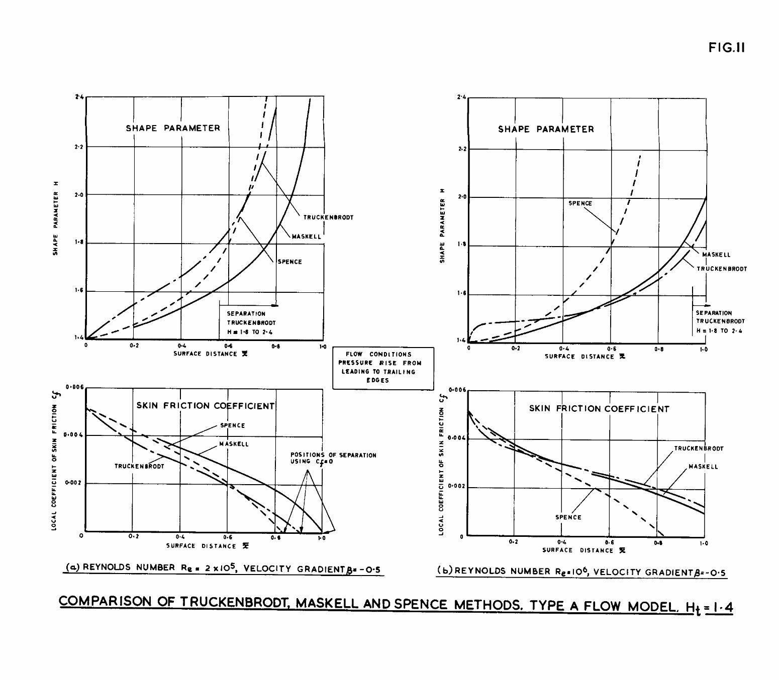
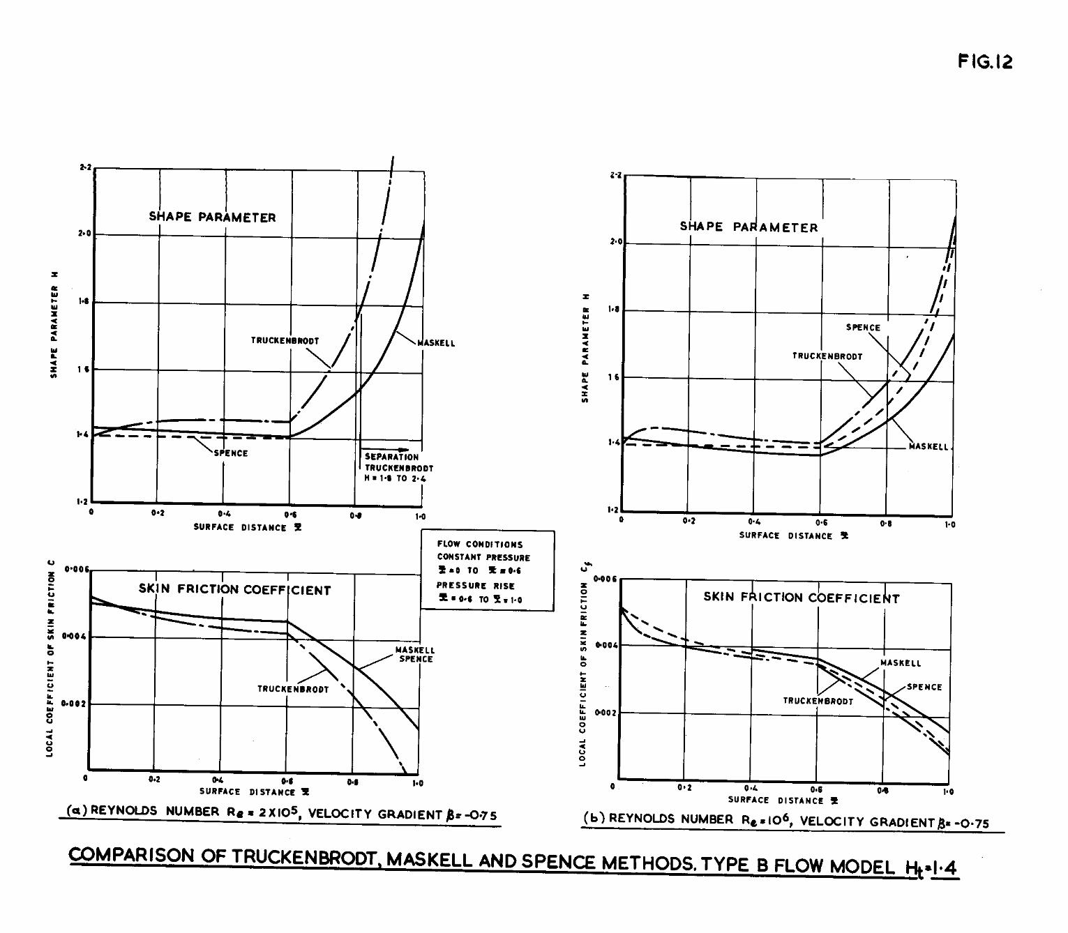
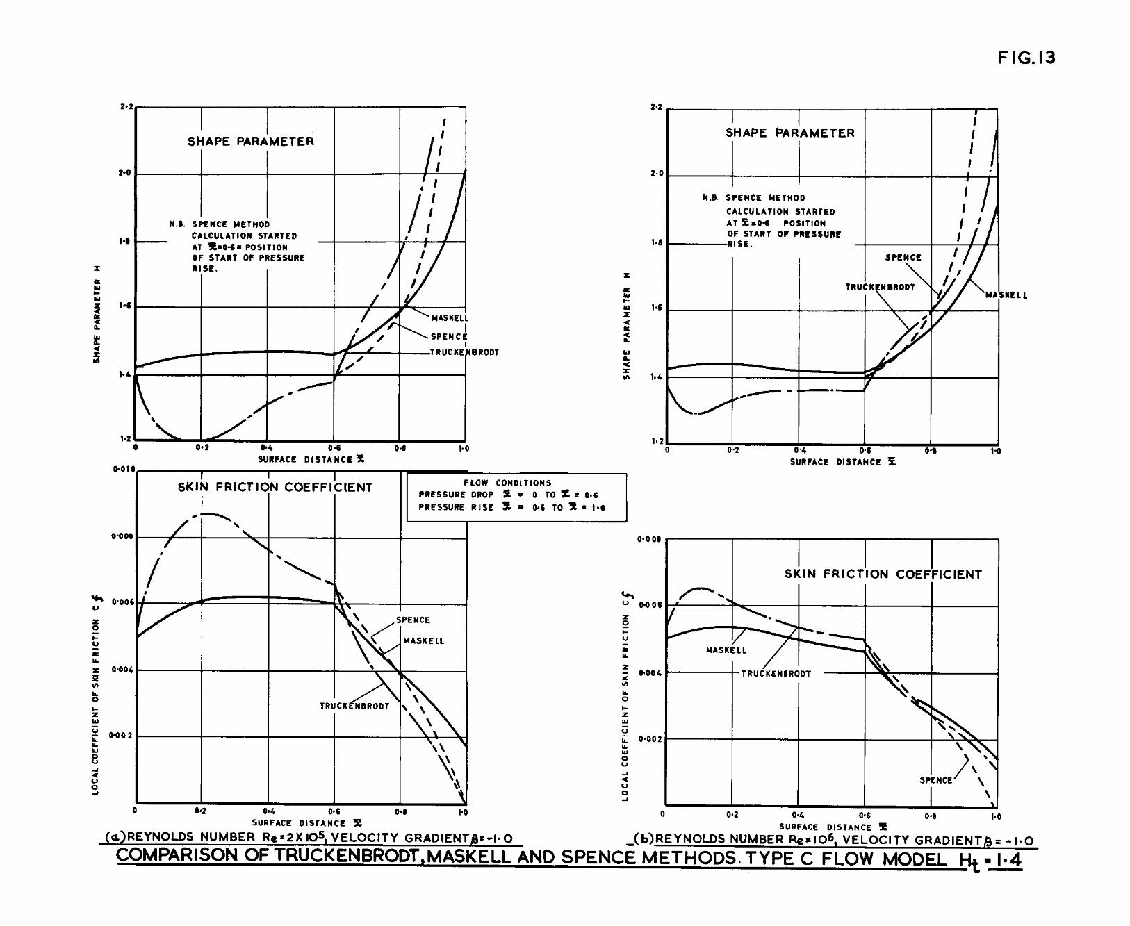
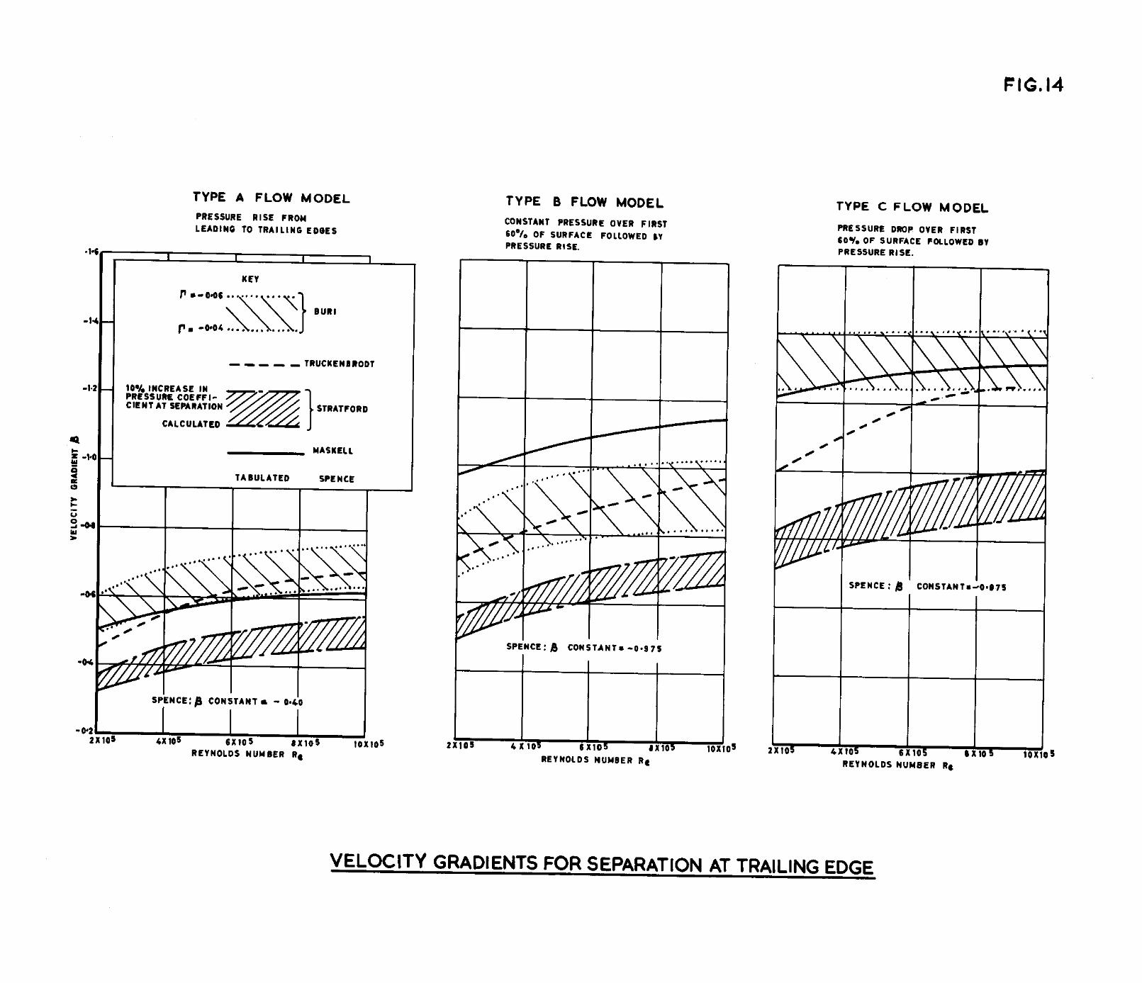
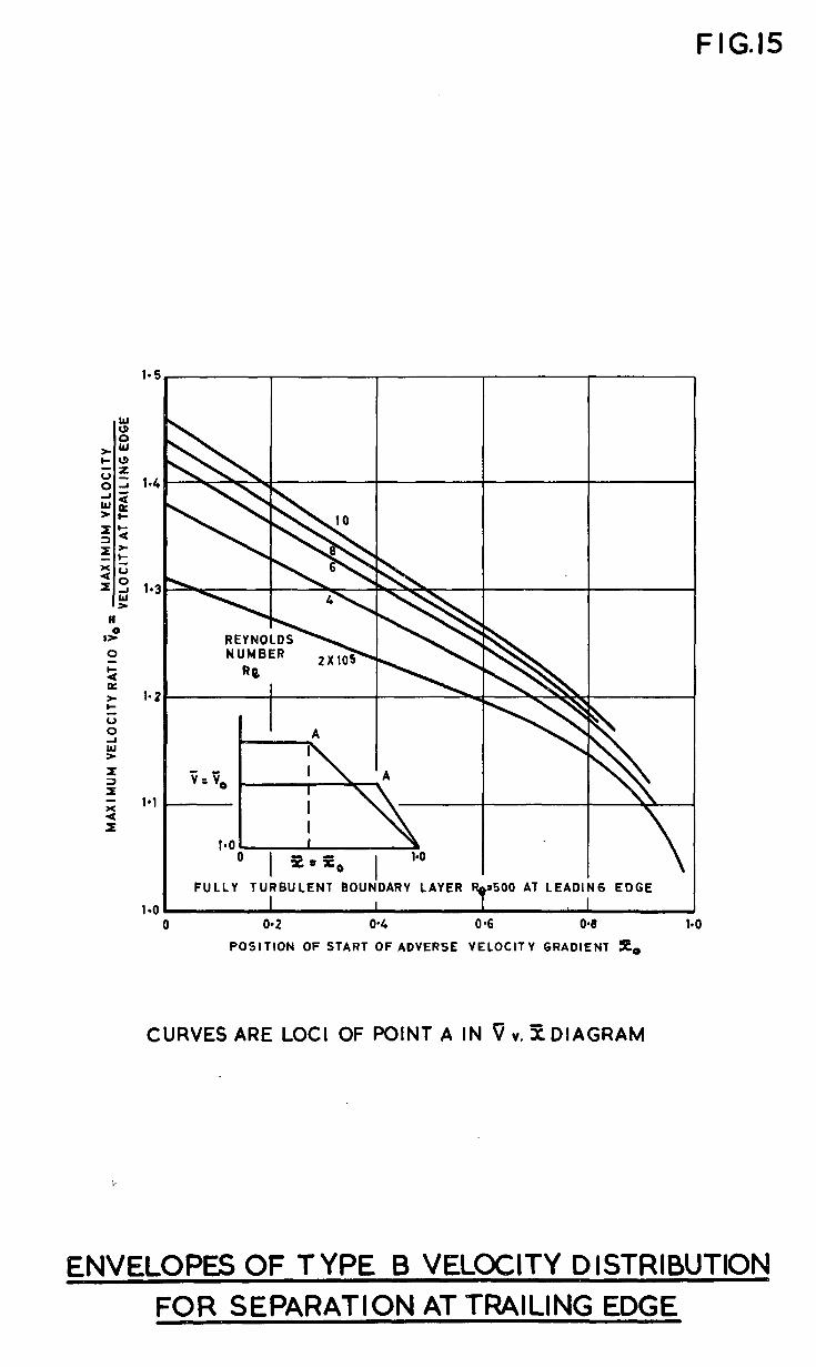
FIG.15

5,

\

\ \

4-

\

4 3-

2-

l-

O-

FULLY TURBULENT BOUNDARY LAYER 500 AT LEADIN EDGE

- - - . - - -- 0 cl*2 0’4 0’6 O*B

POSITION OF START OF ADVERSE VELOCITY GRADIENT x0

CURVES ARE LOCI OF POINT A IN ii v. ZDIAGRAM

ENVELOPES OF TYPE 6 VELOCITY DISTRIBUTION FOR SEPARATION AT TRAILING EDGE

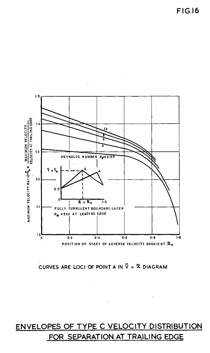
FIG.16

1.2

1-l FULLY TURBULENT BOUNDARY LAYER \ Re ~500 AT LEADING EDGE

0’4 0-b U’U 1.3

POSITION OF START OF ADVERSE VELOCITY GRADIENT f,

CURVES ARE LOCI 0~ POINT A IN V V. Z DIAGRA~v~

ENVELOPES OF TYPE C VELOCITY DISTRIBUTION FOR SEPARATION AT TRAILING EDGE

A.R.C. C.P. No. 868 A.&C. C.P. No. 068 namlb1965 -, 19% Smith, ‘). J. l.. Smith, D. J. L.

- BOUNDARY LAYER TIECIRY AND ITS APPLICATION To BLADE PrOFILE DESIGN

TUABULENP FWNDARY LAYER THWRY AliD ITS APF’LICATION To BLUE PfDFfLE. DESIGN

Five methods oi predict lng the Incompressible, Lwo-dimenslonal turbulerlt bomdary layer have been applled Lo floe conditions consir:ered Lo occur over the suction surface of turbo machine blades and the measure of agteement between the separation criteria and boundary layer charac- ter1stiw assessed. The methods considered were those due Lo hurl, TmckeubrodL, Stratford, tleskell and Spence.

Five methods of predlctlng the lncompresslble, Lwo-dlmenslonal turbulent boundary lE&yer have been applied to Ilow conditions considered LO occur over the suction surface of turbo machlne blades and the measure of agreement between the separation criteria and bouudary layer charac- Leristirs assessed. The methods conslciered were those due to Purl, Truckenbrodt, Stratford, Maskell end Spence.

All of the criteria could be brought lnto tolerable agreement prwldefl that a value or -G 04 was used tor EUri’S criteria and that ror Quckenbrodt snd Spencets methods the posiLi3n ol separatlm was detwlned by the condltlm that local skin Ir ctlon coelf.lcienL is zero. It waq addltlonally necessary in the methods of tfsskell, Truckenbrcdt

rwFRI

All of the crlterla could be brcught lnto tolerable agreement pmvlded that a value or -0.01. was used for Burlis criteria, end that for Truckenbrodt and Spence’s methods the positlan or separation was determined by the condition that local skin rrictlon coefllclent is zero. IL was additionally necessary in the methods oi Maskell, Tmckenbrodt

- .--- --.- -- -- _- .-es-- .-

A.R.C. C.P. No. 868 twch, 1965 Gmlth, D. J. L.

.-!?E@--

WRBJIENT BCUNDARY LAY!ZR THEDRY AND ITS APPLICATION To BL+ADE PRJFILS DESIGN

Five methods ol predicting the lncompresslble, Lwo-dimensloaal turbulent boundary layer have been applled Lo flow conditions considered LO occur over the suet ion surrace Or LUI%O machine blades aud the measure of agreement between the separation criteria and bouudary layer CharaC- Leristics assessed. ‘lhe methods considered were those due to Purl, Ttuckehbrodt, Stratlord, llaskell and SpeKe.

All or the crlLeCta could be brought into tolerable agreement provided Lhat a value or -O-0:1) was used for BurlQ crlterla, and that ror Tnxkenbrodt and Spence~s methods the posit ion or separation WA88 determined by the condltlon that local skln ir!CtlOn COerfiCimt is SerOm It was addltlonally necessary In the methods of tlaskell, Txuckenbx’odt

OVER/ ~- -

and Spence for the calculation of the shape parameter to be started wlth a value or l*I..

All of the crlterla except Spencecs were sensltlve to Reynolds number and showed that an Increase In Reynolds number delays separation.

Stratfordts method ViBs extremely e-sy to apply, was the simplest of the floe and predicted the lovlest pressure rlse to SeparatlOn.

To ass 1st In the design ot blade prof lles, envelopes of suction surface Velocity dlstrlbutlon have been constructed to give . separation at the tralllng edge; these are considered to be conservatively based.

and Spence ior the calculation of the shape parameter to be started with a value of l-4.

All of the crlterla except Spencefs were sensitive to Reynolds number and showed that an Increase In Reynolds number delays aeperatlon.

Stratiordfs method yas extremely easy to apply, was the slmplest or the rive and predicted the lowest pressure rise to separation.

and Spence ror the calculation of the shape parameter to be started with a value 0r 1’4.

All of the crlterla except Spencefs were senslt lve to Reynolds number and showed that an Increase in Reynolds number delays separation.

Stratrord~s method was extremely easy to apply, was the slmplest or the rive and predicted the lowest pressure rise to separation.

To asslst In the design of blade prorlles, envelopes of suction surface velocity dlstrlbutlon have been constructed to give .

separation at the trailing edge; these are considered to be consmat lvely based.

To ssslst in the design of blade proriles, envelopes of suction surface velocity dlstrlbutfon have been COI’IStNCted to give separation at the tralllng edge; these are cons ldered to be conservatively based.

C.P. No. 868

0 Crown copyright 1966

Printed and published by HER MAJESTY’S STATIONERY OFFICE

To be purchased from 49 High Holborn, London w.c.1 423 Oxford Street, London w.1 13~ Castle Street, Edinburgh 2

109 St. Mary Street, Cardiff Brazennose Street, Manchester 2

50 Fairfax Street, Bristol 1 35 Smallbrook, Ringway, Birmingham 5

80 Chichester Street, Belfast 1 or through any bookseller

Printed in England

C.P. No. 86f S.O. Code No. 23-9016-6

Documents

Turbulent Boundary Layer Theory and its Application ' to Blade