Turbulent Boundary-Layer Simulations - FFI · Turbulent Boundary-Layer Simulations ... such as the wake behind buildings and vehicles, ... however they are less eﬃcient for boundary

Turbulent Boundary-Layer Simulations comparison with experiments

-Espen Åkervik

17/16257FFI-RAPPORT

FFI-RAPPORT 17/16257 1

Turbulent Boundary-Layer Simulations

comparison with experiments

Espen Åkervik

Norwegian Defence Research Establishment (FFI) 5 October 2017

2 FFI-RAPPORT 17/16257

Keywords Simulering

Turbulent strømning Fluidmekanikk

FFI-rapport FFI-RAPPORT 17/16257

Project number 1311,394801

ISBN P: 978-82-464-2966-3 E: 978-82-464-2967-0

Approved by Anders Helgeland, Research Manager Janet M. Blatny, Director

Summary

The turbulent flow of gases and liquids plays an important role in a vast range of applications.Examples of this include atmospheric boundary layer flows, vehicles aerodynamics and internalcombustion systems. From a societal security point of view, the dispersion of harmful substancesin the form of aerosols and gases cannot be fully understood without taking turbulent transport intoaccount. In the maritime sector, it is necessary to describe turbulent motion faithfully in order tobe able to predict the hydrodynamic drag and to understand the noise generating mechanisms ofvessels. Similarly, the prediction of aerodynamic drag, which is important to develop drag reduc-ing designs on aircraft and vehicles, would be virtually impossible without detailed knowledge ofturbulent flows.

In many cases it is possible to perform either full scale or model scale measurements to establishknowledge about the turbulent flows. Clearly, measurements have the advantage that there is noneed to model the flow, and real-time data is possible to extract. On the other hand, the data isoften collected in a noisy environment, and generally it is not possible to collect full space data.

The fast development of software and computer power has rendered computer simulation mod-els based on solution of the Navier-Stokes equations an attractive tool to study turbulent flow phe-nomena. Recently, high fidelity techniques such as Large Eddy Simulation (LES) have becomefeasible for ever more complex problems. However, since LES methods require large computa-tional resources, one needs to reduce the computational domain as much as possible. Due to thislimitation, artificial boundary conditions at the upstream boundary of the computational domain areneeded in order to describe the effect of the incoming flow.

This report presents LES results using a synthetic turbulence generator to supply artificial inflowconditions for two high Reynolds number turbulent boundary layer flows. In both cases, measure-ments are available for comparison. The motivation of this report is hence twofold. First, we aimto validate the performance of the Large Eddy Simulation model as a tool to study boundary layerflows. Second, we aim to quantify the performance of the synthetic turbulence generator.

The synthetic turbulence generator performs well for both flows. Although we find that highspatial resolution is needed to obtain a good measure of the skin friction, the large scale structuresare captured even at relatively coarse resolution. This is important since the large scale structuresare essential both in transport of aerosols and in flow noise generation.


Samandrag

Turbulent strømning av gassar og væsker spelar ei viktig rolle innanfor mange ulike bruksområde.Døme på dette er atmosfæriske grensesjikt, aero- og hydrodynamikken til fartøy og miksing i forbren-ningsprosessar. I eit samfunnstryggleiksperspektiv er det til dømes vanskeleg å predikere spreiingav farlige emne i form av gassar og partiklar utan å ta omsyn til turbulent transport. I maritim sektor erdet naudsynt å kunne skildre turbulente rørsler med stor grad av nøyaktigheit for å kunne bereknestrømningsmotstand og strømningsindusert støy både på overflatefartøy, undervassbåtar og tauaantennesystem. På same måte er designoptimering av fly og bilar for å redusere luftmotstand heiltavhengig av god kunnskap om turbulente strømningar.

I mange tilfelle er det mogleg å utføre enten fullskala eller modellskala målekampanjar for å fåkunnskap om turbulens. Ein fordel med målingar er at ein ikkje treng å modellere strømninga, sam-tidig som det er mogleg å ekstrahere sanntidsdata. På den andre sida vert målingar ofte pregaav støy, noko som gjer det vanskeleg å ekstrahere gode data. På grunn av avgrensingar vedmåleteknikk er det generelt heller ikkje mogleg å samle inn alle data ein ønsker.

Den raske utviklinga i programvare og datakapasitet har medført at simuleringsmodellar basertpå løysing av Navier-Stokes-likningar blir stadig meir eigna som verktøy for å studere turbulentestrømningar. Nyleg har det vorte mogleg å bruke nøyaktige metodar, slik som Large Eddy-simulering(LES), på stadig meir komplekse problemstillingar. Sidan LES-metodar krev stor reknekraft, trengein å avgrense berekningsområdet så mykje som mogleg. Ei slik avgrensing gjer at ein vert nøyddtil å anta at den innkomande turbulente strømninga oppfører seg på ein spesiell måte. Ein set altsåkunstige randkrav.

I denne rapporten har LES blitt brukt til å studere to turbulente grensesjikt med høge Reynolds-tal. I begge tilfella har resultat frå vindtunnel vore tilgjengeleg for samanlikning, og i begge tilfella harein syntetisk turbulensgenerator blitt brukt for å skape randvilkår for den innkomande strømninga.

Resultata viser at den syntetiske turbulensgeneratoren fungerer godt for begge strømningane.Sjølv om høg romleg oppløysing er naudsynt for å oppnå gode estimat på veggfriksjonen, vert deistore skalaene i turbulensen godt skildra, til og med for relativt låg oppløysing. Dette er viktig sidandesse strukturane er essensielle både i transport av aerosolar og i støygenerering.


Contents

1 Introduction 7

2 Flow configurations 102.1 The WALLTURB high Reynolds number experiments 112.2 The EnFlo urban dispersion experiments 12

3 Theoretical considerations 143.1 Governing equations 143.2 Numerical modelling 143.3 Statistical measures 153.4 Synthetic inflow boundary conditions 15

4 Results 174.1 Recreating the flow in the WALLTURB LML tunnel 174.2 Recreating the flow in the EnFlo tunnel 22

5 Conclusions 26



1 Introduction

Turbulent flows are encountered in numerous industrial applications, atmospheric sciences andin everyday life. Turbulence is characterised by irregular chaotic motion, where large eddies,or whirls, create smaller eddies, which in turn create even smaller eddies. This process rendersturbulence an efficient mixer of quantities such as heat, moisture, and aerosols. On one handthis leads to increased friction drag on vehicles, and therefore reduced performance, but on theother hand it enables efficient combustion processes. To be able to simulate turbulent motionis therefore essential both to understand and to create design improvements in a vast range ofindustrial applications.

In a turbulent flow, the size of the eddies range from the largest scale in the flow (i.e. thatgiven by the geometry of the problem) down to a size of some millimetres or even micrometers.Generally, in order to simulate turbulent flows numerically, it is necessary to describe the full rangeof scales. This approach is known as Direct Numerical Simulation (DNS). The use of this methodon most practical problems is almost impossible due to the high computational cost. Instead, theindustry standard method builds on the so called Reynolds Averaging procedure, first formulatedby Reynolds (1895), where only the mean flow is resolved, and the effect of the turbulent eddieson the mean flow is modelled. This class of methods is referred to as Reynolds Averaged NavierStokes (RANS) methods. RANS methods has had significant success, especially in boundary layerdominated flows, such as the flow around air planes. However, the success has been limited indescribing separated flows with vortex shedding, such as the wake behind buildings and vehicles,or buoyancy dominated flows, such as dense gas release. Large Eddy Simulation (LES) methodsprovide a means to accurately predict such flows. In LES, only the large eddies of the flow isresolved, whereas the action of the smaller eddies is modelled, thus rendering the method lesscostly than DNS in terms of computational resources. LES methods has proven very well suitedto describe separated flows, however they are less efficient for boundary layer flows. This problemstems from the fact that close to walls, the large eddies are not that large. In fact their size is limitedby the distance to the wall.

In the present work, LES of two boundary layer flows is performed, and the results are comparedto experiments. It may seem contradictory to simulate boundary layer flows with a tool that is notprimarily designed for such a task. However, even in flows dominated by vortex shedding, suchas flow in urban environments or the wake behind vehicles, there will be interactions between theshed vortices and the incoming turbulent boundary layer flow. Therefore, it is essential to validatethe performance of LES as a tool to study boundary layer flows. LES methods for boundary layerflows are in general computationally costly. Therefore, it is beneficial to reduce the size of thecomputational domain as much as possible. Boundary layers develop due to the presence of wallsof objects that are placed in the flow. An example is the flat plate boundary layer flow, where auniform flow impinges on a horizontal flat plate. Close to the leading edge the boundary layer isthin and supports only laminar flow states. Further downstream the boundary layer thickens andthere is a transition to turbulence, followed by a region of fully developed turbulent flow regime.Most practical applications are in the fully developed turbulent regime and therefore it is mainly thisregime that is of interest to simulate. However, if one is to limit the region of interest one arrivesat the following question: What should the time dependent flow at the upstream boundary of thecomputational domain be? It is evident that knowing the mean flow is not sufficient, and neither is


the superposition of the mean flow and random perturbations, since turbulence is correlated bothin time and space. So a follow up question may be: How much do we need to know about theturbulence that we have omitted to simulate?

For spatially homogeneous flows one has the possibility of imposing periodicity in the stream-wise direction, thereby avoiding the problem of inflow conditions altogether. For spatially devel-oping flows, which in industrial applications is the most common case, the simplest choice is toprescribe a laminar flow and introduce disturbances so that the flow naturally undergoes transitionto turbulence. Disturbances may be introduced by tripping from obstacles or by volume forcesmimicking the behaviour of these. This however, will in most cases yield a large computational do-main, resulting in increased computational cost. In addition, it is not clear how well LES methodshandle transition from laminar to turbulent flow regimes.

To introduce boundary conditions that mimic the behaviour of turbulent flows, there are ac-cording to Keating et al. (2004) three groups of methods: Recycling methods, precursor databasesand synthetic turbulence. In addition, there is a class of methods built on systematic manipulationof experimental data.

Recycling methods, originally introduced by Spalart & Leonard (1985); Spalart (1986, 1988),simplified by Lund et al. (1998) and made more robust by Ferrante & Elghobashi (2004), usea modification of the periodic boundary conditions which takes into account the streamwisedevelopment of the flow. For the flat plate boundary layer flow Lund et al. (1998) extractedvelocity data at a given downstream position. The data were rescaled both in inner coordinates (tomatch a desired friction velocity) and outer coordinates (to match a desired thickness and wakelaw). Although shown to give excellent results for the plate boundary layer flow, Keating et al.

(2004) argues that there are drawbacks to the method; the most important being that the inlet mustbe placed in an equilibrium region (lack of generality), the fairly long fetch of the recycling regionand the introduction of spurious periodicity (c.f. Spille-Kohoff & Kaltenbach, 2001).

Precursor databases are built by running separate simulations or experiments to build up thenecessary information to be used as inflow. The precursor simulation is typically performed in aperiodic domain, and a full transverse plane is stored at every time step. The velocity fields arethen rescaled and used as input for the next simulation. The major drawback is that the precursorsimulation may be as costly (in terms of computer power) as the simulation itself. In addition theremay be considerable storage requirements when saving two-dimensional planes at every time stepof a simulation. This method has been used with success in for instance Li et al. (2000), but littleis known about the effects of significant rescaling when the target flow is far from the precursorflow.

The third class is that of synthetic turbulence. It is motivated by lack of generality in thetwo former classes of methods. In essence, the method is built on manipulation of randomnoise added to a mean velocity profile such that statistical moments and spectra resembles thatof a turbulent flow. Several authors have pointed to the fact that the simplest choice, namely toadd uncorrelated (in time and space) noise to mimic turbulent fluctuations, is a particularly badchoice that leads to immediate decay of turbulence (Druault et al., 2004; Keating et al., 2004).One method to obtain some spatial information is to create time series of velocity fluctuations byinverse Fourier transforms of known spectral densities, as was done in Le et al. (1997), where theamplitude of the Fourier modes were drawn randomly. The authors found that the missing phase


information led to a rapid decay of turbulence levels. In later works (Klein et al., 2003; Batten et al.,2004; di Mare et al., 2006; Jarrin et al., 2006), it was recognised that somehow the correlation intime and space should be considered. To further improve the results of the synthetic methods,Spille-Kohoff & Kaltenbach (2001) introduced forcing on successive downstream locations topenalise deviations from a prescribed Reynolds stress profile. In the review of Keating et al.

(2004), the authors use a precursor periodic channel flow to generate a full data set in time andin the cross-flow plane to be used as inflow conditions for a spatially developing channel flow.They filter the full data and find that length scales larger than the integral length scale are theimportant ones to retain. In addition, the authors review the methods of Batten et al. (2004) andSpille-Kohoff & Kaltenbach (2001) and find that while typical synthetic methods require fairlylong adaption region until a reasonable turbulent solution is obtained, the forcing method ofSpille-Kohoff & Kaltenbach (2001) appears to be effective at reducing the adaption length.

In cases where sufficient experimental data is available, one may attempt to rebuild two-dimensional velocity fields with high temporal resolution directly from measurements. Particleimage velocimetry (PIV) may provide two-dimensional snapshots of the flow with limited timeresolution. On the other hand, good time resolution may be achieved by hot-wire probes, but atthe cost of limited spatial resolution. In Perret et al. (2008), data from a rake of hot-wire probesis used to extract coherent structures from the flow by use of a proper orthogonal decomposition(POD). The authors build a reduced system of the flow using a Galerkin projection onto thebasis of POD modes. The performance was limited by the need to retain only a few modes tokeep the reduced system stable. In Druault et al. (2004), the authors devise a technique based onlinear stochastic estimation. Their method relies on the knowledge of two-point correlations (PODmodes) and high-fidelity time series at three points in space. The former can be obtained by ahot-wire rake or by PIV, whereas the latter may be obtained from hot-wire probes. A version ofthe method developed by Bonnet et al. (1994); Druault et al. (2004) has been successfully usedat FFI to reproduce experimental results for a high Reynolds number turbulent boundary layerflow (see Wingstedt et al., 2013). In that work, the coherent structures were extracted from PIVmeasurements and the time signals needed for the linear stochastic estimation were taken from ahot-wire rake.

In this report, a synthetic turbulence generator, similar to the method of Klein et al. (2003), isused to generate artificial inflow conditions based on limited experimental data for two differenthigh Reynolds number boundary layer flows. The structure of the report is as follows. In Chapter2, both the experimental and the numerical set up of the two flow cases are presented. In Chapter3, the theoretical considerations are presented. The results are reported in Chapter 4. Concludingremarks are given in Chapter 5.


0 1 2 3 4 5 6 7 8 9 10

210

0

0.5

1

1.5

2

x/δ (downstream )

flow direction

z/δ (transverse)

y/δ

(wal

l nor

mal

)

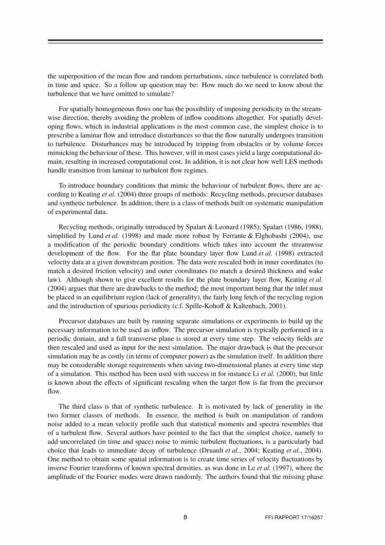
Figure 2.1 Illustration of the computational box for boundary layer flows. All lengths in the illustration

are normalised by the boundary layer height δ.

2 Flow configurations

In this report, two different turbulent boundary layer flow configurations are considered. Figure2.1 shows the basic setup. At the inflow a time varying synthetic velocity field is prescribed,defining a unidirectional freestream flow U∞ flowing over a wall. Towards the wall, the flow isdecelerated due to viscous shear forces, thereby defining a boundary layer of thickness δ. Since theimposed inflow boundary conditions are not true solutions to the Navier–Stokes equations, therewill be an adaptation region some distance downstream of the inflow, where some disturbancesare dampened, while others are amplified. Results from the simulations are compared to resultsobtained from wind tunnel experiments. Table 2.1 describes the relevant parameters defining thedifferent cases. Case A was computed as a baseline flat plate boundary-layer flow to comparewith turbulent flow over linear surface waves in the project FFI project “Maritime BoundaryLayers”. The simulation parameters are set to match experimental data from the WALLTURBproject (Delville et al., 2009). Case B is a boundary layer flow to be used as inflow data (precursorsimulation) for dispersion modelling in the European Defence Agency (EDA) funded “MODITIC”project. Here, the numerical setup matches the setup of the EnFlo wind tunnel in Surrey. Thecomputational grid used in each of the flows are given in Table 2.2 and the next sections describethe two experiments in more detail.

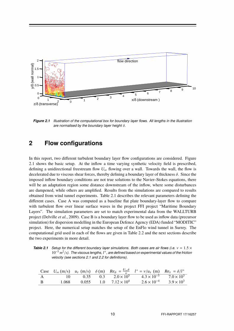
Table 2.1 Setup for the different boundary layer simulations. Both cases are air flows (i.e. ν = 1.5 ×10−5 m2/s). The viscous lengths, l+, are defined based on experimental values of the friction

velocity (see sections 2.1 and 2.2 for definitions).

Case U∞ (m/s) uτ (m/s) δ (m) Reδ =U∞δ

νl+ = ν/uτ (m) Reτ = δ/l+

A 10 0.35 0.3 2.0 × 105 4.3 × 10−5 7.0 × 103

B 1.068 0.055 1.0 7.12 × 104 2.6 × 10−4 3.9 × 103


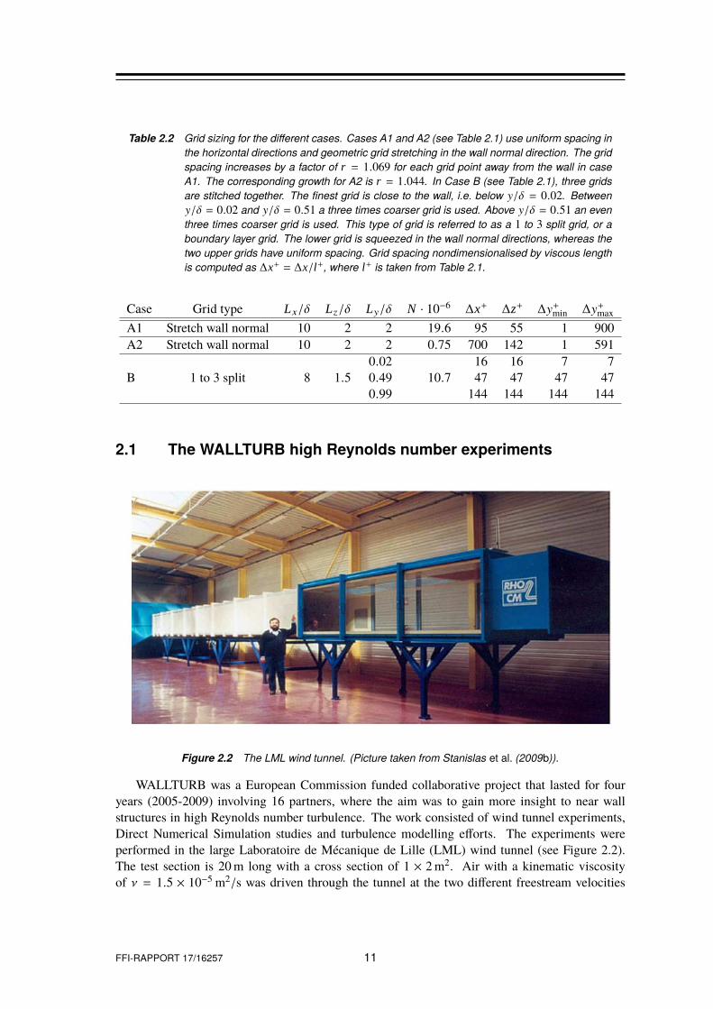
Table 2.2 Grid sizing for the different cases. Cases A1 and A2 (see Table 2.1) use uniform spacing in

the horizontal directions and geometric grid stretching in the wall normal direction. The grid

spacing increases by a factor of r = 1.069 for each grid point away from the wall in case

A1. The corresponding growth for A2 is r = 1.044. In Case B (see Table 2.1), three grids

are stitched together. The finest grid is close to the wall, i.e. below y/δ = 0.02. Between

y/δ = 0.02 and y/δ = 0.51 a three times coarser grid is used. Above y/δ = 0.51 an even

three times coarser grid is used. This type of grid is referred to as a 1 to 3 split grid, or a

boundary layer grid. The lower grid is squeezed in the wall normal directions, whereas the

two upper grids have uniform spacing. Grid spacing nondimensionalised by viscous length

is computed as ∆x+ = ∆x/l+, where l+ is taken from Table 2.1.

Case Grid type Lx/δ Lz/δ Ly/δ N · 10−6∆x+ ∆z+ ∆y

+

min ∆y+

max

A1 Stretch wall normal 10 2 2 19.6 95 55 1 900A2 Stretch wall normal 10 2 2 0.75 700 142 1 591

B 1 to 3 split 8 1.50.02

10.716 16 7 7

0.49 47 47 47 470.99 144 144 144 144

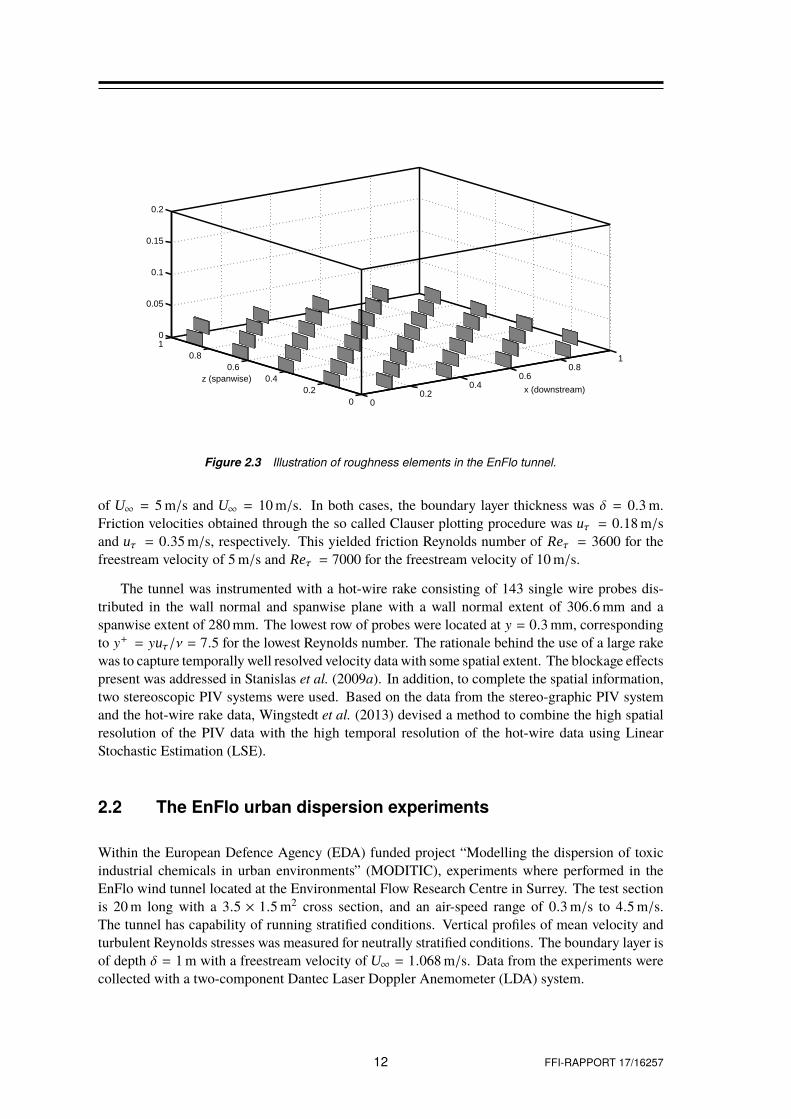
2.1 The WALLTURB high Reynolds number experiments

Figure 2.2 The LML wind tunnel. (Picture taken from Stanislas et al. (2009b)).

WALLTURB was a European Commission funded collaborative project that lasted for fouryears (2005-2009) involving 16 partners, where the aim was to gain more insight to near wallstructures in high Reynolds number turbulence. The work consisted of wind tunnel experiments,Direct Numerical Simulation studies and turbulence modelling efforts. The experiments wereperformed in the large Laboratoire de Mécanique de Lille (LML) wind tunnel (see Figure 2.2).The test section is 20 m long with a cross section of 1 × 2 m2. Air with a kinematic viscosityof ν = 1.5 × 10−5 m2/s was driven through the tunnel at the two different freestream velocities


00.2

0.40.6

0.81

00.2

0.40.6

0.810

0.05

0.1

0.15

0.2

x (downstream)z (spanwise)

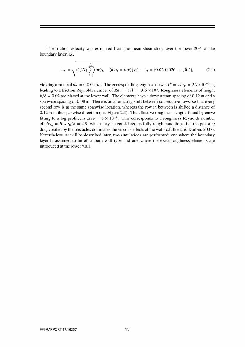
Figure 2.3 Illustration of roughness elements in the EnFlo tunnel.

of U∞ = 5 m/s and U∞ = 10 m/s. In both cases, the boundary layer thickness was δ = 0.3 m.Friction velocities obtained through the so called Clauser plotting procedure was uτ = 0.18 m/sand uτ = 0.35 m/s, respectively. This yielded friction Reynolds number of Reτ = 3600 for thefreestream velocity of 5 m/s and Reτ = 7000 for the freestream velocity of 10 m/s.

The tunnel was instrumented with a hot-wire rake consisting of 143 single wire probes dis-tributed in the wall normal and spanwise plane with a wall normal extent of 306.6 mm and aspanwise extent of 280 mm. The lowest row of probes were located at y = 0.3 mm, correspondingto y

+= yuτ/ν = 7.5 for the lowest Reynolds number. The rationale behind the use of a large rake

was to capture temporally well resolved velocity data with some spatial extent. The blockage effectspresent was addressed in Stanislas et al. (2009a). In addition, to complete the spatial information,two stereoscopic PIV systems were used. Based on the data from the stereo-graphic PIV systemand the hot-wire rake data, Wingstedt et al. (2013) devised a method to combine the high spatialresolution of the PIV data with the high temporal resolution of the hot-wire data using LinearStochastic Estimation (LSE).

2.2 The EnFlo urban dispersion experiments

Within the European Defence Agency (EDA) funded project “Modelling the dispersion of toxicindustrial chemicals in urban environments” (MODITIC), experiments where performed in theEnFlo wind tunnel located at the Environmental Flow Research Centre in Surrey. The test sectionis 20 m long with a 3.5 × 1.5 m2 cross section, and an air-speed range of 0.3 m/s to 4.5 m/s.The tunnel has capability of running stratified conditions. Vertical profiles of mean velocity andturbulent Reynolds stresses was measured for neutrally stratified conditions. The boundary layer isof depth δ = 1 m with a freestream velocity of U∞ = 1.068 m/s. Data from the experiments werecollected with a two-component Dantec Laser Doppler Anemometer (LDA) system.


The friction velocity was estimated from the mean shear stress over the lower 20% of theboundary layer, i.e.

uτ =

√√

√

(1/N )N∑

i=1

〈uv〉i, 〈uv〉i = 〈uv〉(yi), yi = {0.02, 0.026, . . . , 0.2}, (2.1)

yielding a value of uτ = 0.055 m/s. The corresponding length scale was l+ = ν/uτ = 2.7×10−5 m,leading to a friction Reynolds number of Reτ = δ/l+ = 3.6 × 103. Roughness elements of heighth/δ = 0.02 are placed at the lower wall. The elements have a downstream spacing of 0.12 m and aspanwise spacing of 0.08 m. There is an alternating shift between consecutive rows, so that everysecond row is at the same spanwise location, whereas the row in between is shifted a distance of0.12 m in the spanwise direction (see Figure 2.3). The effective roughness length, found by curvefitting to a log profile, is z0/δ = 8 × 10−4. This corresponds to a roughness Reynolds numberof Rez0 = Reτ z0/δ = 2.9, which may be considered as fully rough conditions, i.e. the pressuredrag created by the obstacles dominates the viscous effects at the wall (c.f. Ikeda & Durbin, 2007).Nevertheless, as will be described later, two simulations are performed; one where the boundarylayer is assumed to be of smooth wall type and one where the exact roughness elements areintroduced at the lower wall.


3 Theoretical considerations

3.1 Governing equations

Generally, the motion of fluids can be described by a set of conservation equations along with anumber of constitutive relations describing the material properties of the fluid. We here considerincompressible Newtonian fluids for which the motion is governed by conservation of mass andmomentum (Kundu et al., 2012)

∇ · u = 0,

ρ (∂tu + u · ∇u) = ∇ · σ,(3.1)

where u = u(x, y, z, t) is the velocity vector in all three spatial directions, ρ is the density and σthe stress tensor. For Newtonian fluids, the constitutive relation, linking the flow gradients to thestresses, is expressed as

σ = −pI + 2µs. (3.2)

Here, p is the pressure acting normal to any surface, µ is the dynamic viscosity and s is the strainrate tensor

s =12

(

∇u + (∇u)T)

. (3.3)

The set of equations (3.1) are referred to as the Navier–Stokes equations for incompressibleNewtonian flow. The equations need suitable initial and boundary conditions to be solved. Later,the subject of inflow boundary conditions will be discussed in more detail.

3.2 Numerical modelling

The Navier–Stokes equations need to be solved numerically, since exact solutions only exist forvery simplified problems. The presence of turbulence renders the direct numerical solution (DNS)difficult due to the large range of both spatial and temporal scales that need to be described. Onepossible method is to use a Large Eddy Simulation (LES) technique, where formally the equationsare filtered to keep only the low frequency part of the spectrum, i.e. discarding the smallest scalesin the problem (Sagaut, 2006). The filtering operation leads to extra unclosed advection terms.The resulting terms can be written as a tensor adding to the stress tensor in eq. (3.1)

σ = −pI + 2µs + σSGS, (3.4)

which describes the effect of the neglected small scale fluctuations on the resolved flow field. Thetask is now to model the tensor σSGS in terms of resolved variables. In the dynamic Smagorinskysub-grid scale viscosity model, where the effect of the unresolved small scales are modelled as“viscous” effects, one writes

σSGS = −2νSGSs, with νSGS = νSGS(x, t). (3.5)


The sub-grid viscosity in the dynamic Smagorinsky model is computed from the resolved strainrate s and the grid size of the problem. Further details on LES theory and methodology, as wellas the computational route to finding the eddy-viscosity, can be found in e.g. Pope (2000); Sagaut(2006).

In this report, we use a Finite Volume Method based LES solver developed at Cascade Tech-nologies (Mahesh et al., 2002; Ham & Iaccarino, 2004; Mahesh et al., 2004; Ham et al., 2006). Itis second-order accurate in space and up to second order accurate in time, and a fractional step pres-sure correction method is applied to enforce divergence free solutions. Applications to turbulentproblems at FFI using Large Eddy Simulation are found in Wingstedt et al. (2013); Rashid et al.

(2011); Vik et al. (2015); Vartdal (2016); Wingstedt et al. (2016) and in the PhD thesis of Fossum(2015) and the papers therein.

3.3 Statistical measures

The resolved flow fields can be decomposed into mean and fluctuating parts, i.e. u = U + u′,p = P+ p′. Here, upper-case symbols (U and P) denote averaged fields, whereas lower-case primesymbols represent fluctuations around the mean. All averages reported in this work are averagedin time and spanwise (z) direction. For instance, for the velocity field we write

U(x, y) = 〈u(x, t)〉 = L−1z T−1

av

∫ Tav

0

∫ Lz

0u(x, t)dzdt, (3.6)

in which 〈·〉 denotes the averaging operator. The Reynolds stresses are defined as

R(x, y) = 〈u′(x, t)u′(x, t)〉 =

〈u′1u′1〉〈u′1u′2〉〈u

′1u′3〉

〈u′2u′1〉〈u′2u′2〉〈u

′2u′3〉

〈u′3u′1〉〈u′3u′2〉〈u

′3u′3〉

, (3.7)

which is a symmetric, i.e. R = RT , covariance matrix. The Reynolds stresses represent one-pointone-time correlations, which provide local information on the statistics. To obtain informationon the spatial structure of the flow the simplest statistical measure is the two-point one-time autocovariance (Pope, 2000)

R(r, x, y) = 〈u′(x, t)u′(x + r, t)〉, (3.8)

which for r = 0 reduces to the standard one-point one-time correlations. The streamwise integrallength scale may then be defined as

L11(x, y) =1

R11(0, x, y)

∫ ∞

0R11(rx, x, y)drx, (3.9)

and the other directions are defined similarly. Two-time one-point statistics can be defined byintroducing a time lag instead of a distance in Equation (3.8), i.e. R(τ, x, y) = 〈u′(x, t)u′(x, t + τ)〉.

3.4 Synthetic inflow boundary conditions

Consider a rectangular box of size Lx × Ly × Lz (see Figure 2.1). The mean flow is in the x−direction, with inflow at x = 0 and outflow at x = Lx . The wall is located at y = 0, and at y = Ly


the presence of the wall should not be felt. The z direction is a transverse homogeneous direction(with respect to the wall and the direction of the freestream) and can be treated as periodic. Arequirement is that the length Lz should be sufficiently large to capture the relevant structures ofthe flow. For the flat plate boundary layer flow this corresponds to a few transverse integral lengthscales. At the lower wall, where y = 0, no-slip conditions are enforced. At the outflow boundary,x = Lx , an advective scheme is imposed, ensuring that structures propagate out of the domainwith minimal reflections. Note that a couple of boundary layer thicknesses upstream of the outflowboundary, the results are usually affected by the boundary condition, and this region should bediscarded from analyses. At the top of the computational domain (y = Ly) the task is to truncatethe “infinite” domain in the wall normal direction. To accommodate a growing boundary layerin an incompressible flow, entrainment of fluid from above is needed. In the present work, we aapply a slip condition at the top. This effectively means that there is no entrainment of fluid. Theboundary layer thickness can hence not be expected to develop correctly downstream. Instead, onecan view the resulting flow field as a frozen downstream position with sufficient spatial extent forlarge scale turbulent structures to exist. Care has to be taken that the domain is sufficiently high tominimise the acceleration of the fluid.

The inflow boundary conditions at x = 0 is by far the most challenging to determine, sincethis requires knowledge about the incoming turbulent flow. When simulating a boundary layerflow using the Reynolds Averaged Navier-Stokes (RANS) equations only mean flow conditions,Ui (y, z), are necessary to impose. However, when using Direct Numerical Simulation (DNS) orLarge Eddy Simulation (LES), one needs to introduce also the time varying fluctuations u′

i(y, z, t).

These fluctuations u′i(y, z, t) should be prescribed in such a way that the flow downstream develops

as fast as possible into a reasonable turbulent field without actually having to solve the full problem,i.e. without simulating the incoming turbulent flow. In the code from Cascade Technologies, asynthetic turbulence generator based on filtering of white noise in Fourier space is used. Thismethod is similar to the method of Klein et al. (2003); di Mare et al. (2006). Recently, also asynthetic turbulence generator based on differential filtering of randomly generated signals inphysical space was added to the code. However, in this report we only consider the former method.


4 Results

4.1 Recreating the flow in the WALLTURB LML tunnel

In the WALLTURB project, turbulent boundary layer flows were studied for a range of freestreamvelocities. We seek here to reproduce the flow with a freestream velocity of U∞ = 10 m/s. Forthis case, the authors of Delville et al. (2009) report a boundary layer thickness of δ = 0.3 m and afriction velocity of uτ = 0.35 m/s, leading to a friction Reynolds number of Reτ = Uτδ/ν = 7000.Note that the exact determination of the friction velocity is in general challenging when analysingexperimental results. However, in the present experiment, the three methods of Clauser plot, PIVand oil-film interferometry yielded very similar results. Hence, one can conclude that the obtainedestimate of the friction velocity is rather good. The viscous length scale computed based on thefriction velocity is l+ = ν/uτ = 4.3 × 10−5 m.

To generate suitable inflow boundary conditions, the mean and the Reynolds stress profilesare used in conjunction with the digital filter synthetic turbulence generator. There are two freeparameters to be set; namely an estimate of the transverse integral length scale and an estimate ofthe streamwise integral time scale. In the PhD thesis of Tutkun (2008), the author gives estimatesof these quantities for this specific flow, and finds that the transverse integral length scale growsmonotonically from approximately Li

z/δ = 0.02 close to the wall to approximately Liz/δ = 0.15 at

the top of the boundary layer. The streamwise integral time scale increases from T ixU∞/δ = 0.15

close to wall to T ixU∞/δ = 0.5 at y/δ = 0.13. Thereafter, it decreases to T i

xU∞/δ = 0.3 at the top ofthe boundary layer. Following Keating et al. (2004), who recommended to retain the largest lengthscales, we choose a slightly higher value of the transverse integral length scale of Li

z/δ = 0.2.The integral time scale is set to T i

xU∞/δ = 0.2, which is in the lower part of the range reported inTutkun (2008). The influence of the choice of integral length and time scales will be discussedlater.

Two computational grids are considered. The details of the computational grids are given inTable 2.2 as case A1 for the fine grid and A2 for the coarse grid. For case A1, the computationalgrid has dimensions Lx × Ly × Lz = 10δ × 2δ × 2δ, whereas for case A2 the dimensions areLx × Ly × Lz = 10δ × 2δ × δ The horizontal grid resolution for case A1 (A2) is ∆x+ = 95 (700),∆z+ = 55 (142) in the streamwise and spanwise direction, respectively. In the wall normaldirection, both case A1 and A2 use grid stretching with geometric growth from the wall to thetop of the domain. In both cases the first grid point is located at y

+= 1 (corresponding to

y/δ = 1.42 × 10−4). The geometric growth factor is r = 1.069 for case A1, and r = 1.044 for caseA2. For case A1 this yields a grid spacing of 439 l+ at the top of the boundary layer (y/δ = 1)and 900 l+ in the dynamically less import freestream at y/δ = 2. It has been verified using thehorizontal resolution as in case A2, by varying the wall normal resolution, that the relatively largevertical grid spacing used in case A1 in the wall normal direction at the top of the domain has nosignificant effect on the statistics. Simulations are performed in two stages. Initially a period ofTU∞/δ = 50 inertial times is simulated to achieve a statistically steady state of the flow variables,starting from an interpolated coarse grid result. Subsequently, a second simulation is performedfor a period of TU∞/δ = 220 inertial time units to gather statistics. For case A1, the skin frictionstatistics varied by a factor of 0.05% for the last 100 time units, which is an indication of wellconverged statistics.


0 2 4 6 8 100

0.1

0.2

0.3

0.4

0.5

0.6

0.7

0.8

0.9

1

x/δ

uτ/uex

pτ

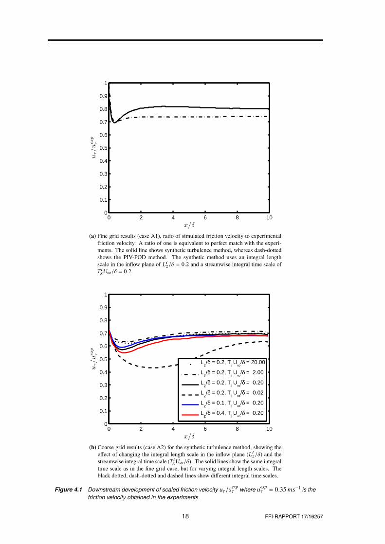
(a) Fine grid results (case A1), ratio of simulated friction velocity to experimentalfriction velocity. A ratio of one is equivalent to perfect match with the experi-ments. The solid line shows synthetic turbulence method, whereas dash-dottedshows the PIV-POD method. The synthetic method uses an integral lengthscale in the inflow plane of Li

z/δ = 0.2 and a streamwise integral time scale ofT ixU∞/δ = 0.2.

0 2 4 6 8 100

0.1

0.2

0.3

0.4

0.5

0.6

0.7

0.8

0.9

1

x/δ

uτ/uex

pτ

Lz/δ = 0.2, T

i U∞/δ = 20.00

Lz/δ = 0.2, T

i U∞/δ = 2.00

Lz/δ = 0.2, T

i U∞/δ = 0.20

Lz/δ = 0.2, T

i U∞/δ = 0.02

Lz/δ = 0.1, T

i U∞/δ = 0.20

Lz/δ = 0.4, T

i U∞/δ = 0.20

(b) Coarse grid results (case A2) for the synthetic turbulence method, showing theeffect of changing the integral length scale in the inflow plane (Li

z/δ) and thestreamwise integral time scale (T i

xU∞/δ). The solid lines show the same integraltime scale as in the fine grid case, but for varying integral length scales. Theblack dotted, dash-dotted and dashed lines show different integral time scales.

Figure 4.1 Downstream development of scaled friction velocity uτ/uexpτ where uexp

τ = 0.35 ms−1 is the

friction velocity obtained in the experiments.


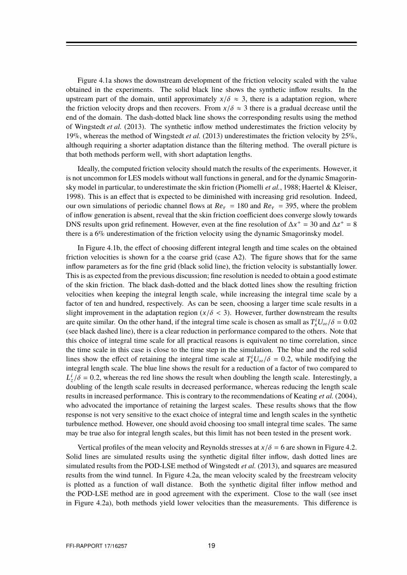
Figure 4.1a shows the downstream development of the friction velocity scaled with the valueobtained in the experiments. The solid black line shows the synthetic inflow results. In theupstream part of the domain, until approximately x/δ ≈ 3, there is a adaptation region, wherethe friction velocity drops and then recovers. From x/δ ≈ 3 there is a gradual decrease until theend of the domain. The dash-dotted black line shows the corresponding results using the methodof Wingstedt et al. (2013). The synthetic inflow method underestimates the friction velocity by19%, whereas the method of Wingstedt et al. (2013) underestimates the friction velocity by 25%,although requiring a shorter adaptation distance than the filtering method. The overall picture isthat both methods perform well, with short adaptation lengths.

Ideally, the computed friction velocity should match the results of the experiments. However, itis not uncommon for LES models without wall functions in general, and for the dynamic Smagorin-sky model in particular, to underestimate the skin friction (Piomelli et al., 1988; Haertel & Kleiser,1998). This is an effect that is expected to be diminished with increasing grid resolution. Indeed,our own simulations of periodic channel flows at Reτ = 180 and Reτ = 395, where the problemof inflow generation is absent, reveal that the skin friction coefficient does converge slowly towardsDNS results upon grid refinement. However, even at the fine resolution of ∆x+ = 30 and ∆z+ = 8there is a 6% underestimation of the friction velocity using the dynamic Smagorinsky model.

In Figure 4.1b, the effect of choosing different integral length and time scales on the obtainedfriction velocities is shown for a the coarse grid (case A2). The figure shows that for the sameinflow parameters as for the fine grid (black solid line), the friction velocity is substantially lower.This is as expected from the previous discussion; fine resolution is needed to obtain a good estimateof the skin friction. The black dash-dotted and the black dotted lines show the resulting frictionvelocities when keeping the integral length scale, while increasing the integral time scale by afactor of ten and hundred, respectively. As can be seen, choosing a larger time scale results in aslight improvement in the adaptation region (x/δ < 3). However, further downstream the resultsare quite similar. On the other hand, if the integral time scale is chosen as small as T i

xU∞/δ = 0.02(see black dashed line), there is a clear reduction in performance compared to the others. Note thatthis choice of integral time scale for all practical reasons is equivalent no time correlation, sincethe time scale in this case is close to the time step in the simulation. The blue and the red solidlines show the effect of retaining the integral time scale at T i

xU∞/δ = 0.2, while modifying theintegral length scale. The blue line shows the result for a reduction of a factor of two compared toLiz/δ = 0.2, whereas the red line shows the result when doubling the length scale. Interestingly, a

doubling of the length scale results in decreased performance, whereas reducing the length scaleresults in increased performance. This is contrary to the recommendations of Keating et al. (2004),who advocated the importance of retaining the largest scales. These results shows that the flowresponse is not very sensitive to the exact choice of integral time and length scales in the syntheticturbulence method. However, one should avoid choosing too small integral time scales. The samemay be true also for integral length scales, but this limit has not been tested in the present work.

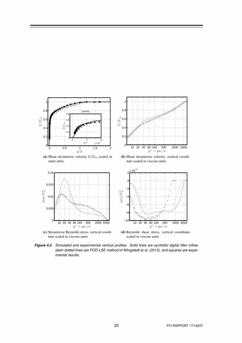
Vertical profiles of the mean velocity and Reynolds stresses at x/δ = 6 are shown in Figure 4.2.Solid lines are simulated results using the synthetic digital filter inflow, dash dotted lines aresimulated results from the POD-LSE method of Wingstedt et al. (2013), and squares are measuredresults from the wind tunnel. In Figure 4.2a, the mean velocity scaled by the freestream velocityis plotted as a function of wall distance. Both the synthetic digital filter inflow method andthe POD-LSE method are in good agreement with the experiment. Close to the wall (see insetin Figure 4.2a), both methods yield lower velocities than the measurements. This difference is


0 0.5 1 1.5 20

0.2

0.4

0.6

0.8

1

y/δ

U/U∞

0 5 10

x 10−3

0

0.2

0.4

0.6

0.8

y/δ

U/U∞

(zoom)

(a) Mean streamwise velocity U/U∞ scaled inouter units.

10 20 40 80 160 500 2000 60000

0.2

0.4

0.6

0.8

1

y+ = yuτ/ν

U/U∞

(b) Mean streamwise velocity, vertical coordi-nate scaled in viscous units.

10 20 40 80 160 500 2000 60000

0.005

0.01

0.015

0.02

y+ = yuτ/ν

〈uu〉/U

2 ∞

(c) Streamwise Reynolds stress, vertical coordi-nate scaled in viscous units

10 20 40 80 160 500 2000 6000−10

−8

−6

−4

−2

0

2x 10

−4

y+ = yuτ/ν

〈uv〉/U

2 ∞

(d) Reynolds shear stress, vertical coordinatescaled in viscous units

Figure 4.2 Simulated and experimental vertical profiles. Solid lines are synthetic digital filter inflow,

dash-dotted lines are POD-LSE method of Wingstedt et al. (2013), and squares are exper-

imental results.


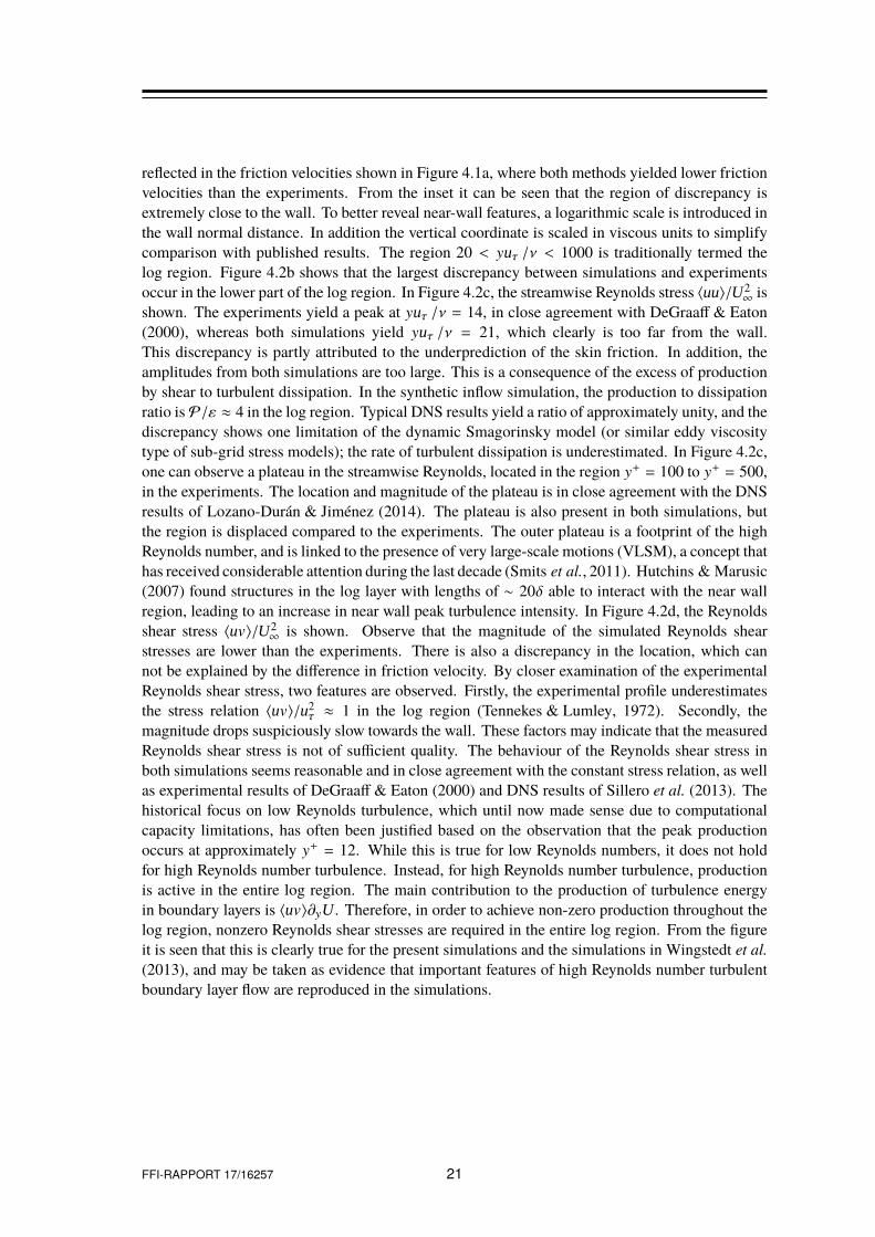
reflected in the friction velocities shown in Figure 4.1a, where both methods yielded lower frictionvelocities than the experiments. From the inset it can be seen that the region of discrepancy isextremely close to the wall. To better reveal near-wall features, a logarithmic scale is introduced inthe wall normal distance. In addition the vertical coordinate is scaled in viscous units to simplifycomparison with published results. The region 20 < yuτ /ν < 1000 is traditionally termed thelog region. Figure 4.2b shows that the largest discrepancy between simulations and experimentsoccur in the lower part of the log region. In Figure 4.2c, the streamwise Reynolds stress 〈uu〉/U2

∞ isshown. The experiments yield a peak at yuτ /ν = 14, in close agreement with DeGraaff & Eaton(2000), whereas both simulations yield yuτ /ν = 21, which clearly is too far from the wall.This discrepancy is partly attributed to the underprediction of the skin friction. In addition, theamplitudes from both simulations are too large. This is a consequence of the excess of productionby shear to turbulent dissipation. In the synthetic inflow simulation, the production to dissipationratio is P/ε ≈ 4 in the log region. Typical DNS results yield a ratio of approximately unity, and thediscrepancy shows one limitation of the dynamic Smagorinsky model (or similar eddy viscositytype of sub-grid stress models); the rate of turbulent dissipation is underestimated. In Figure 4.2c,one can observe a plateau in the streamwise Reynolds, located in the region y

+= 100 to y

+= 500,

in the experiments. The location and magnitude of the plateau is in close agreement with the DNSresults of Lozano-Durán & Jiménez (2014). The plateau is also present in both simulations, butthe region is displaced compared to the experiments. The outer plateau is a footprint of the highReynolds number, and is linked to the presence of very large-scale motions (VLSM), a concept thathas received considerable attention during the last decade (Smits et al., 2011). Hutchins & Marusic(2007) found structures in the log layer with lengths of ∼ 20δ able to interact with the near wallregion, leading to an increase in near wall peak turbulence intensity. In Figure 4.2d, the Reynoldsshear stress 〈uv〉/U2

∞ is shown. Observe that the magnitude of the simulated Reynolds shearstresses are lower than the experiments. There is also a discrepancy in the location, which cannot be explained by the difference in friction velocity. By closer examination of the experimentalReynolds shear stress, two features are observed. Firstly, the experimental profile underestimatesthe stress relation 〈uv〉/u2

τ≈ 1 in the log region (Tennekes & Lumley, 1972). Secondly, the

magnitude drops suspiciously slow towards the wall. These factors may indicate that the measuredReynolds shear stress is not of sufficient quality. The behaviour of the Reynolds shear stress inboth simulations seems reasonable and in close agreement with the constant stress relation, as wellas experimental results of DeGraaff & Eaton (2000) and DNS results of Sillero et al. (2013). Thehistorical focus on low Reynolds turbulence, which until now made sense due to computationalcapacity limitations, has often been justified based on the observation that the peak productionoccurs at approximately y

+= 12. While this is true for low Reynolds numbers, it does not hold

for high Reynolds number turbulence. Instead, for high Reynolds number turbulence, productionis active in the entire log region. The main contribution to the production of turbulence energyin boundary layers is 〈uv〉∂yU. Therefore, in order to achieve non-zero production throughout thelog region, nonzero Reynolds shear stresses are required in the entire log region. From the figureit is seen that this is clearly true for the present simulations and the simulations in Wingstedt et al.

(2013), and may be taken as evidence that important features of high Reynolds number turbulentboundary layer flow are reproduced in the simulations.


4.2 Recreating the flow in the EnFlo tunnel

To reproduce the boundary layer flow from the EnFlo tunnel described in Section 2.2, two caseshave been simulated. In the wind tunnel, the flow is subject to the combined effects of the turbulentair produced by the fan, the vortex generators, and the obstacles on the floor. To isolate the effectof the roughness obstacles, both a smooth wall boundary and a rough wall boundary layer flowhave been simulated, and in both cases, synthetic inflow conditions were used at the upstreamboundary. In the synthetic method, the two main input parameters (apart from mean velocityprofiles and Reynolds stresses) are the integral length scales in the inflow plane and the integraltime scale in the streamwise direction. The integral length scales were set so as to define a series ofpiecewise constant profiles with parameters derived from the experiments (see Table 4.1). Buildingon the hypothesis of Keating et al. (2004), that the large scales are the most important to retain,a simulation with uniform integral length and time scale of Li

z = 0.6 and T ix = 0.6 was also

performed. For the present case, although the statistics far downstream agree well between the twocases, the adaptation region was shorter when using varying length and time scales.

Table 4.1 Setup of integral length and time scales for the EnFlo simulations. The integral length scale

is set to piecewise constant in intervals ranging from y0/δ to y1/δ.

y0/δ y1/δ Liz/δ T i

xU∞/δ

0 0.05 0.15 0.30.05 0.1 0.25 0.420.1 0.4 0.45 0.560.4 0.9 0.3 0.330.9 1.5 0.2 0.2

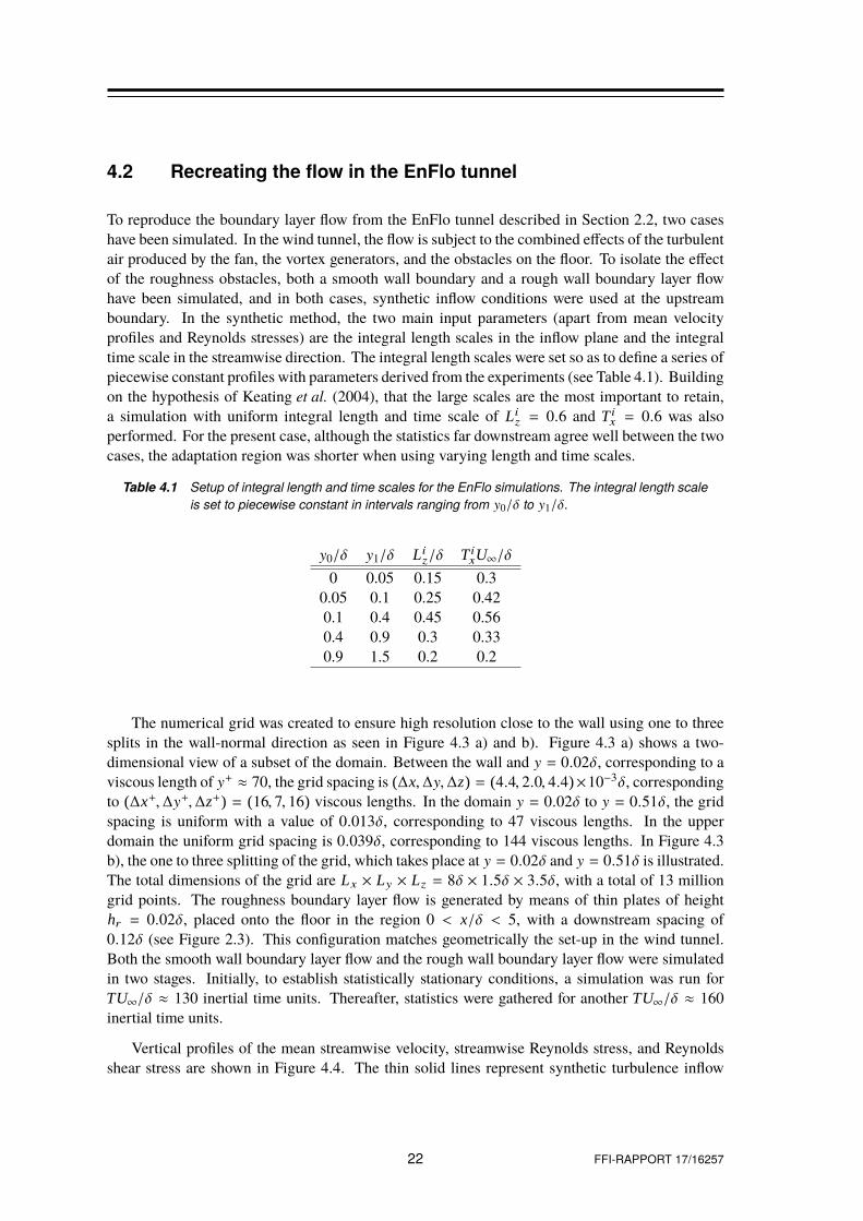
The numerical grid was created to ensure high resolution close to the wall using one to threesplits in the wall-normal direction as seen in Figure 4.3 a) and b). Figure 4.3 a) shows a two-dimensional view of a subset of the domain. Between the wall and y = 0.02δ, corresponding to aviscous length of y+ ≈ 70, the grid spacing is (∆x,∆y,∆z) = (4.4, 2.0, 4.4)×10−3δ, correspondingto (∆x+,∆y+,∆z+) = (16, 7, 16) viscous lengths. In the domain y = 0.02δ to y = 0.51δ, the gridspacing is uniform with a value of 0.013δ, corresponding to 47 viscous lengths. In the upperdomain the uniform grid spacing is 0.039δ, corresponding to 144 viscous lengths. In Figure 4.3b), the one to three splitting of the grid, which takes place at y = 0.02δ and y = 0.51δ is illustrated.The total dimensions of the grid are Lx × Ly × Lz = 8δ × 1.5δ × 3.5δ, with a total of 13 milliongrid points. The roughness boundary layer flow is generated by means of thin plates of heighthr = 0.02δ, placed onto the floor in the region 0 < x/δ < 5, with a downstream spacing of0.12δ (see Figure 2.3). This configuration matches geometrically the set-up in the wind tunnel.Both the smooth wall boundary layer flow and the rough wall boundary layer flow were simulatedin two stages. Initially, to establish statistically stationary conditions, a simulation was run forTU∞/δ ≈ 130 inertial time units. Thereafter, statistics were gathered for another TU∞/δ ≈ 160inertial time units.

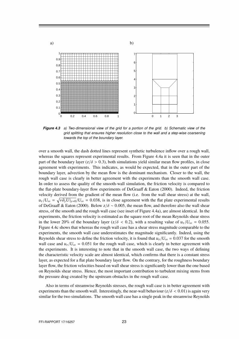
Vertical profiles of the mean streamwise velocity, streamwise Reynolds stress, and Reynoldsshear stress are shown in Figure 4.4. The thin solid lines represent synthetic turbulence inflow


a) b)

0 0.2 0.4 0.6 0.8 10

0.1

0.2

0.3

0.4

0.5

0.6

0.7

0.8

0.9

1

0 1 2 30

1

2

3

4

5

6

7

Figure 4.3 a) Two-dimensional view of the grid for a portion of the grid. b) Schematic view of the

grid splitting that ensures higher resolution close to the wall and a step-wise coarsening

towards the top of the boundary layer.

over a smooth wall, the dash dotted lines represent synthetic turbulence inflow over a rough wall,whereas the squares represent experimental results. From Figure 4.4a it is seen that in the outerpart of the boundary layer (z/δ > 0.3), both simulations yield similar mean flow profiles, in closeagreement with experiments. This indicates, as would be expected, that in the outer part of theboundary layer, advection by the mean flow is the dominant mechanism. Closer to the wall, therough wall case is clearly in better agreement with the experiments than the smooth wall case.In order to assess the quality of the smooth-wall simulation, the friction velocity is compared tothe flat-plate boundary-layer flow experiments of DeGraaff & Eaton (2000). Indeed, the frictionvelocity derived from the gradient of the mean flow (i.e. from the wall shear stress) at the wall,uτ/U∞ =

√

ν∂yU |y=0/U∞ = 0.038, is in close agreement with the flat plate experimental resultsof DeGraaff & Eaton (2000). Below z/δ ∼ 0.005, the mean flow, and therefore also the wall shearstress, of the smooth and the rough wall case (see inset of Figure 4.4a), are almost identical. In theexperiments, the friction velocity is estimated as the square root of the mean Reynolds shear stressin the lower 20% of the boundary layer (z/δ < 0.2), with a resulting value of uτ/U∞ = 0.055.Figure 4.4c shows that whereas the rough wall case has a shear stress magnitude comparable to theexperiments, the smooth wall case underestimates the magnitude significantly. Indeed, using theReynolds shear stress to define the friction velocity, it is found that uτ/U∞ = 0.037 for the smoothwall case and uτ/U∞ = 0.051 for the rough wall case, which is clearly in better agreement withthe experiments. It is interesting to note that in the smooth wall case, the two ways of definingthe characteristic velocity scale are almost identical, which confirms that there is a constant stresslayer, as expected for a flat plate boundary layer flow. On the contrary, for the roughness boundarylayer flow, the friction velocities based on wall shear stress is significantly lower than the one basedon Reynolds shear stress. Hence, the most important contribution to turbulent mixing stems fromthe pressure drag created by the upstream obstacles in the rough wall case.

Also in terms of streamwise Reynolds stresses, the rough wall case is in better agreement withexperiments than the smooth wall. Interestingly, the near-wall behaviour (z/δ < 0.01) is again verysimilar for the two simulations. The smooth wall case has a single peak in the streamwise Reynolds


0 0.2 0.4 0.6 0.8 10

0.10.20.30.40.50.60.70.80.9

11.1

y/δ

U/U

∞

0 0.02 0.04−0.2

0

0.2

0.4

0.6

0.8

y/δ

U/U∞

(zoom)

(a) Mean streamwise velocity U/U∞

0 0.2 0.4 0.60

0.005

0.01

0.015

0.02

y/δ

〈uu〉/U

2 ∞

(b) Streamwise Reynolds stress 〈uu〉/U2∞

0 0.2 0.4 0.6−5

−4

−3

−2

−1

0x 10

−3

y/δ

〈uv〉/U

2 ∞

(c) Reynolds shear stress 〈uv〉/U2∞

Figure 4.4 Simulated and experimental vertical profiles. Solid lines are smooth wall synthetic inflow,

dash-dotted lines are rough wall synthetic inflow, and squares are experimental results.


stress, located slightly below z/δ = 0.015 (about 20 wall units). The rough wall case on the otherhand, has a double peak behaviour, with the first peak being almost identical to the smooth wallcase, both in location and magnitude, and the second peak located at z/δ = 0.1. The inner peakis related to viscous mechanisms, whereas the outer peak is related to turbulence produced by theaerodynamic drag of the obstacles.

To conclude, even at the relatively small roughness Reynolds number in the present case, itis necessary to include the geometric effects of the roughness elements in the wind tunnel inorder to reproduce the flow numerically. Although the smooth wall simulation fails to provide agood representation of the wind tunnel results, it is seen to be in good agreement with flat plateexperiments. This may be taken as evidence of the satisfactory performance of the syntheticturbulence generator and the Large Eddy Simulation code.


5 Conclusions

In this report, Large Eddy Simulation of two high Reynolds number turbulent boundary layerflows, where measurements are available for comparison, has been performed. The motivationfor the study is twofold. First, to check the performance of our Large Eddy Simulation code as atool to study wall bounded flows. Second, to assess the quality of the synthetic inflow generatorwhich is implemented in the code. Indeed, one key issue to address when performing high fidelitytechniques such as Direct Numerical or Large Eddy Simulation for turbulent boundary layers, isthe need to introduce artificial time dependent boundary conditions at the upstream edge of thecomputational domain. Since one is limited by available computational resources, it is of interestto reduce the size of the domain considered as much as possible. To achieve this one needs toprescribe the behaviour of the flow at the inlet. In this report, we have considered the use of a digitalfilter based synthetic turbulence generator, where the mean velocity and Reynolds stress profiles areprescribed at the inflow. Based on this information together with estimates of length and time scalesin the flow, a time varying “synthetic” turbulence field is generated by manipulation of randomnoise. Naturally, these type of methods produce unphysical results some distance downstream ofthe inlet, and one main interest is to evaluate the length of the adaptation region. Another issueis related to how well the simulated turbulent flows perform in terms of comparison with realisticflows.

The first flow studied is a high Reynolds turbulent boundary layer flow with a slight favourablepressure gradient. We find that there is a downstream adaptation region of approximately threeboundary layer thicknesses. Previously, adaptation lengths of approximately 20 boundary layerthicknesses have been reported (Klein et al., 2003; di Mare et al., 2006; Keating et al., 2004),but those results have typically been for lower Reynolds numbers, where the intrinsic instabilitymechanisms are weaker. It is interesting to note that the method of Wingstedt et al. (2013) hasan adjustment region of only two boundary layer thicknesses, which is impressive. However, inthat method the friction velocity stabilises at a lower level than in the synthetic turbulence method.In terms of Reynolds stresses the two methods perform similarly. Given the similar behaviour ofthe two methods and that the synthetic turbulence method requires less input data, the syntheticturbulence would be the method of choice for general flow situations where limited knowledge isavailable.

The second flow studied is a boundary layer flow over a rough wall. In the experiment,the incoming turbulent flow is produced by the combined effect of a fan and large scale vortexgenerators. As the flow enters the test section, it interacts with small obstacles at the floor, tocreate a boundary layer flow that is reminiscent of that in the atmospheric boundary layer. Toisolate the effect of the wall obstacles, two simulations are performed, both of which use syntheticinflow turbulence imposed at the upstream boundary. In the first simulation, a smooth lower wallis used, whereas in the second simulation a rough lower wall, matching geometrically the set up inthe experiment, is used. The rough wall simulation is in excellent agreement with the experiment,clearly outperforming the smooth wall simulation. This shows that the dynamical relevance ofthe obstacles at the lower wall is significant. Although the smooth wall simulation provide flowprofiles that are in poor agreement with the experimental results, the flow adapts fairly quickly(within four boundary layer thicknesses) to a well behaved smooth wall turbulent boundary layerflow, in close agreement with published smooth wall results. The digital filter synthetic inflow


generator is therefore seen to perform well as a tool to introduce artificial turbulent flow fields atthe upstream boundary.

Large Eddy Simulation of turbulent boundary layer flows is a challenging task due to strictresolution requirements close to the wall, where the flow is dominated by viscous mechanisms.Therefore, in order to obtain a good measure of the skin friction, high resolution is needed. Onthe other hand, the large scale structures, present only in high Reynolds number flows, are wellreproduced in the simulations, even at relatively coarse resolution.

Acknowledgements

This work was funded by the Norwegian Research Council (NFR) RENERGI programme, grantnumber KPN-216465, “Fluid Structure Interactions for Wind Turbines” (FSI-WT) and by theEuropean Defence Agency (EDA) project B-1097-ESM4-GP “Modelling the dispersion of toxicindustrial chemicals in urban environments” (MODITIC). Some simulations were performed onthe computational resources at NTNU provided by NOTUR, www.sigma2.no. The rough wallsimulation was performed by Daniel Eriksson.


Bibliography

Batten, P., Goldberg, U. & Chakravarthy, S. 2004 Interfacing Statistical Turbulence ClosuresWith Large-Eddy Simulation. AIAA journal 42 (3), 485–492.

Bonnet, J.P., Cole, D.R., Delville, J., Glauser, M.N. & Ukeiley, L.S. 1994 Stochastic Es-timation and Proper Orthogonal Decomposition: Complementary Techniques for IdentifyingStructure. Exp. Fluids 17 (5), 307–314.

DeGraaff, D. B. & Eaton, J. K. 2000 Reynolds Number Scaling of The Flat-Plate TurbulentBoundary Layer. J. Fluid Mech. 422, 319–346.

Delville, J., Braud, P., Coudert, S., Foucaut, J.-M., Fourment, C., George, W. K., Johansson,P. B. V., Kostas, J., Mehdi, F., Royer, A., Stanislas, M. & Tutkun, M. 2009 The WALL-TURB Joined Experiment To Assess The Large Scale Structures In A High Reynolds NumberTurbulent Boundary Layer. In Progress In Wall Turbulence: Understanding and Modelling (ed.M. Stanislas, J. Jimenez & I. Marusic).

Druault, P., Lardeau, S., Bonnet, J.-P., Coiffet, F., Delville, J., Lamballais, E., Largeau,J.-F. & Perret, L. 2004 Generation of Three-Dimensional Turbulent Inlet Conditions for Large-Eddy Simulation. AIAA J. 42 (3), 447–456.

Ferrante, A. & Elghobashi, S. E. 2004 A Robust Method for Generating Inflow Conditionsfor Direct Numerical Simulations of Spatially-Developing Turbulent Boundary Layers. J. Comp

Phys. 198, 372–287.

Fossum, H. 2015 Computational Modeling of Stably Stratified, Turbulent Shear Flows. PhD thesis,Department of Mathematics, University of Oslo.

Haertel, C. & Kleiser, L. 1998 Analysis and Modelling of Subgrid-Scale Motions in Near-WallTurbulence. J. Fluid Mech. 356, 327–352.

Ham, F. & Iaccarino, G. 2004 Energy Conservation In Collocated Discretization Schemes onUnstructured Meshes. Annual Research Briefs 2004, 3–14.

Ham, F., Mattsson, K. & Iaccarino, G. 2006 Accurate and Stable Finite Volume Operators ForUnstructured Flow Solvers. Tech. Rep.. Center For Turbulence Research (CTR).

Hutchins, N. & Marusic, I. 2007 Evidence of Very Long Meandering Features in the LogarithmicRegion of Turbulent Boundary Layers. J. Fluid Mech. 579, 1–28.

Ikeda, T. & Durbin, P. A. 2007 Direct Simulations of Rough-Wall Channel Flow. J. Fluid Mech.

571, 235–263.

Jarrin, N., Benhamadouche, S., Laurence, D. & Prosser, R. 2006 A Synthetic-Eddy-MethodFor Generating Inflow Conditions For Large-Eddy Simulations. Int. J. Heat Fluid 27 (4), 585–593.

Keating, A., Piomelli, U., Balaras, E. & Kaltenbach, H.-J. 2004 A Priori and A PosterioriTests of Inflow Conditions For Large-Eddy Simulation. Phys. Fluids 16, 4696.


Klein, M., Sadiki, A. & Janicka, J. 2003 A Digital Filter Based Generation of Inflow DataFor Spatially Developing Direct Numerical or Large Eddy Simulations. J. Comp Phys. 186 (2),652–665.

Kundu, P. K., Cohen, I. M. & Dowling, D. R. 2012 Fluid Mechanics, 5th edn. Elsevier AcademicPress.

Le, H., Moin, P. & Kim, J. 1997 Direct Numerical Simulation of Turbulent Flow Over A Backward-Facing Step. J. Fluid Mech. 330, 349–374.

Li, N., Balaras, E. & Piomelli, U. 2000 Inflow Conditions For Large-Eddy Simulations ofMixing Layers. Phys. Fluids 12, 935.

Lozano-Durán, Adrián & Jiménez, Javier 2014 Effect of the computational domain on directsimulations of turbulent channels up to re τ= 4200. Phys. Fluids 26, 011702.

Lund, T. S, Wu, X. & Squires, K. D. 1998 Generation of Turbulent Inflow Data For Spatially-Developing Boundary Layer Simulations. J. Comp Phys. 140 (2), 233–258.

Mahesh, K., Constantinescu, G., Apte, S., Iaccarino, G., Ham, F. & Moin, P. 2002 ProgressToward Large-Eddy Simulation of Turbulent Reacting and Non-Reacting Flows In ComplexGeometries. Annual Research Briefs pp. 115–142.

Mahesh, K., Constantinescu, G. & Moin, P. 2004 A Numerical Method For Large-Eddy Simu-lation In Complex Geometries. J. Comp Phys. 197, 215–240.

di Mare, L, Klein, M, Jones, WP & Janicka, J 2006 Synthetic Turbulence Inflow Conditions forLarge-Eddy Simulation. Phys. Fluids 18, 025107.

Perret, L., Delville, J., Manceau, R. & Bonnet, J.-P. 2008 Turbulent Inflow Conditions ForLarge-Eddy Simulation Based On Low-Order Empirical Model. Phys. Fluids 20, 075107.

Piomelli, U., Ferziger, J. & Moin, P. 1988 Model Consistency in Large Eddy Simulation ofTurbulent Channel Flows. Phys. Fluids 31, 1884.

Pope, S. B. 2000 Turbulent Flows. Cambridge, United Kingdom: Cambridge University Press.

Rashid, F., Vartdal, M. & Grue, J. 2011 Oscillating Cylinder In Viscous Fluid: Calculation ofFlow Patterns and Forces. J. Eng. Math. 70 (1-3), 281–295.

Reynolds, O. 1895 On the Dynamical Theory of Incompressible Viscous Fluids and the Deter-mination of the Criterion. Phil. Trans. R. Soc. A. 168, 123–164.

Sagaut, P. 2006 Large Eddy Simulation For Incompressible Flows: An Introduction, 3rd edn.Springer.

Sillero, Juan A, Jiménez, Javier & Moser, Robert D 2013 One-point statistics for turbulentwall-bounded flows at reynolds numbers up to δ+ ≈ 2000. Phys. Fluids 25, 105102.

Smits, A. J., McKeon, B. J. & Marusic, I. 2011 High-Reynolds Number Wall Turbulence. Annu.

Rev. Fluid Mech. 43, 353–375.

Spalart, P. R. 1986 Numerical Study of Sink-Flow Boundary Layers. J. Fluid Mech. 172, 307–328.


Spalart, P. R. 1988 Direct Simulation of A Turbulent Boundary Layer Up To Reθ= 1410. J. Fluid

Mech. 187, 61–98.

Spalart, P. R. & Leonard, A. 1985 Direct Numerical Simulation of Equilibrium TurbulentBoundary Layers. In 5th Symposium on Turbulent Shear Flows, , vol. 1, p. 9.

Spille-Kohoff, A. & Kaltenbach, H.-J. 2001 Generation of Turbulent Inflow Data With APrescribed Shear-Stress Profile. Tech. Rep.. DTIC Document.

Stanislas, M., Foucaut, J.-M., Coudert, S., Tutkun, M., George, W. K. & Delville, J. 2009a

Calibration of The WALLTURB Experiment Hot Wire Rake With Help of PIV. In Progress In

Wall Turbulence: Understanding and Modelling (ed. M. Stanislas, J. Jimenez & I. Marusic).

Stanislas, M., Jimenez, J. & Marusic, I., ed. 2009b Progress In Wall Turbulence: Understanding

and Modelling. Springer.

Tennekes, H. & Lumley, J. L. 1972 A First Course in Turbulence. MIT Press.

Tutkun, M. 2008 Structure of Zero Pressure Gradient High Reynolds Number Turbulent Bound-ary Layers. PhD thesis, Division of Fluid Mech., Dept. App. Mech., Chalmers University ofTechnology.

Vartdal, M. 2016 Computing Turbulence Structure Tensors in Plane Channel Flow. Computers

& Fluids 136, 207–211.

Vik, T., Tørnes, J. A. & Reif, B. A. P. 2015 Simulations of the Release and Dispersion of Chlorineand Comparison with the Jack Rabbit Field Trials. Tech. Rep. 01474. FFI, Norwegian DefenceResearch Establishment.

Wingstedt, E. M. M., Osnes, A. N., Åkervik, E., Eriksson, D. & Reif, B. A. P. 2016 Large-EddySimulation of Dense Gas Dispersion Over A Simplified Urban Area. Atm Env 251, 605–616.

Wingstedt, E. M. M., Vartdal, M., Osnes, A. N. & Tutkun, M. 2013 Development of LESInflow Conditions For Turbulent Boundary Layers. Tech. Rep. 02420. FFI, Norwegian DefenceResearch Establishment.


About FFIThe Norwegian Defence Research Establishment (FFI) was founded 11th of April 1946. It is organised as an administrative agency subordinate to the Ministry of Defence.

FFI’s mIssIonFFI is the prime institution responsible for defence related research in Norway. Its principal mission is to carry out research and development to meet the require-ments of the Armed Forces. FFI has the role of chief adviser to the political and military leadership. In particular, the institute shall focus on aspects of the development in science and technology that can influence our security policy or defence planning.

FFI’s vIsIonFFI turns knowledge and ideas into an efficient defence.

FFI’s chArActerIstIcsCreative, daring, broad-minded and responsible.

om FFIForsvarets forskningsinstitutt ble etablert 11. april 1946. Instituttet er organisert som et forvaltnings organ med særskilte fullmakter underlagt Forsvarsdepartementet.

FFIs FormålForsvarets forskningsinstitutt er Forsvarets sentrale forskningsinstitusjon og har som formål å drive forskning og utvikling for Forsvarets behov. Videre er FFI rådgiver overfor Forsvarets strategiske ledelse. Spesielt skal instituttet følge opp trekk ved vitenskapelig og militærteknisk utvikling som kan påvirke forutsetningene for sikkerhetspolitikken eller forsvarsplanleggingen.

FFIs vIsjonFFI gjør kunnskap og ideer til et effektivt forsvar.

FFIs verdIerSkapende, drivende, vidsynt og ansvarlig.

FFI’s organisation

Forsvarets forskningsinstituttPostboks 25 2027 Kjeller

Besøksadresse:Instituttveien 202007 Kjeller

Telefon: 63 80 70 00Telefaks: 63 80 71 15Epost: [email protected]

Norwegian Defence Research Establishment (FFI)P.O. Box 25NO-2027 Kjeller

Office address:Instituttveien 20 N-2007 Kjeller

Telephone: +47 63 80 70 00 Telefax: +47 63 80 71 15 Email: [email protected]

Documents

Turbulent Boundary-Layer Simulations - FFI · Turbulent Boundary-Layer Simulations ... such as the wake behind buildings and vehicles, ... however they are less eﬃcient for boundary