PTT työpapereita 191 PTT Working Papers 191

Assessment of the EC cyclical adjustment methodology for Finland – impact on budget

balances Janne Huovari, Signe Jauhiainen ja Antti Kekäläinen

Helsinki 2017

2

PTT työpapereita 191

PTT Working Papers 191

ISBN 978-952-224-202-0 (pdf)

ISSN 1796-4784 (pdf)

Pellervon taloustutkimus PTT

Pellervo Economic Research PTT

Helsinki 2017

3

Janne Huovari, Signe Jauhiainen ja Antti Kekäläinen. 2017. Euroopan komission suhdan-

nekorjausmenetelmän arviointi Suomelle – vaikutus rakenteelliseen jäämään. PTT työ-

papereita 191.

Tiivistelmä: Tässä työpaperissa arvioimme, millaiselta Euroopan komission talouden ja rahoituksen pääosaston tekemä julkisen talouden rakenteellisen jäämän estimointi näyt-tää Suomen tapauksessa. Rakenteellinen jäämä saadaan nimellisestä jäämästä vähentä-mällä siitä suhdannekomponentti ja kertaluonteiset erät. Komission suhdannekorjaus-menetelmässä suhdannekomponentti muodostuu rahoitusaseman puolijoustosta ja tuo-tantokuilusta. Raportissa tarkastellaan komission menetelmää, jotta voidaan paremmin ymmärtää siihen liittyvien oletusten vaikutuksia Suomelle. Arviot Suomen tuotantokui-lusta vaihtelevat suuresti eri oletuksista riippuen – erityisesti työttömyyden trendin ja osallistumisasteen erilaisilla oletuksilla on merkitystä. Tämä vaihtelu näkyy myös suhdan-nekorjatussa jäämässä. Joustoarviotkin ovat herkkiä erisuuruisille tuotantokuilun esti-maateille, mutta joustojen vaikutus rahoitusasemaan vaihtelevien tuotantokuiluarvioiden kautta on suhteellisen pieni. Julkisen talouden ohjausta ja arviointia koskeva säännöstö edellyttää selkeää menetelmää suhdannekorjatun jäämän arvioimiseksi. Komission me-netelmä ei täytä näitä kriteerejä, joten olisi parempi pitää sitä neuvoa-antavana välineenä kuin sitovana sääntönä.

Asiasanat: suhdannekorjattu jäämä, tuotantokuilu, julkisen talouden ohjaus

Janne Huovari, Signe Jauhiainen ja Antti Kekäläinen. 2017. Assessment of the EC cyclical

adjustment methodology for Finland – impact on budget balances. PTT Working Papers

191.

Abstract: In this paper, we assess how the cyclical adjustment of budget balances em-ployed by the European Commission (EC) DG ECFIN performs in the case of Finland. The CAB can be obtained from the actual budget balance-to-GDP ratio by subtracting an estimated cyclical component from it. In the EC cyclical adjustment methodology, the cyclical component is composed of the budgetary semi-elasticity and the output gap esti-mate. The aim of the study is to scrutinise the EC methodology to be able to better under-stand the implications of assumptions made about its different components within the context of Finland. The findings show that the Finnish output gap estimates vary greatly with varying assumptions, especially with the different assumptions made on the trend unemployment and the participation rate. The variation is also reflected in the CAB. The elasticity estimates are sensitive to different estimates of the output gap, but the effect of the elasticity on the CAB through varying output gaps is still relatively small. The rules regarding fiscal surveillance and governance impose a need for a robust methodology when evaluating the CAB. The EC methodology does not meet that criteria, and it would be better to ascribe it a consultative role rather than a role as a binding rule.

Keywords: cyclical adjustment of budget balance, output gap, fiscal surveillance.

4

The research was financed by the National Audit Office of Finland. We would like to

thank Jenni Jaakkola, Arto Kokkinen, Tero Kuusi, Matti Okko and Seppo Orjasniemi for

their valuable comments as well as the participants of the Workshop on Structural Bal-

ance – Uncertainty of Potential Output and Policy Implications organised in Helsinki in

March 2017.

5

Contents

1 Introduction ....................................................................................................................... 6

2 Methodology ....................................................................................................................... 8

2.1 Description of the methodology ............................................................................... 8

2.2 Budgetary semi-elasticity ......................................................................................... 10

2.3 Previous literature on the evaluation of the methodology .................................. 11

3 Testing the components of the potential GDP ............................................................. 12

3.1 Production function parameters ............................................................................. 13

3.2 Working age population, participation rate and average hours worked ........... 14

3.3 Unemployment rate ................................................................................................. 20

3.3.1 Overview of potential unemployment rate estimation ................................ 21

3.3.2 NAWRU model specification: Phillips curve ................................................ 23

3.3.3 NAWRU model specification: cycle and trend state equations and their

estimation.......................................................................................................................... 25

3.3.4 Forecast with anchoring................................................................................... 30

3.3.5 Mean-adjustment of NAWRU ........................................................................ 31

3.4 TFP ............................................................................................................................. 32

3.4.1 TFP trend assumptions .................................................................................... 33

3.4.2 TFP cycle assumption in transition equation ............................................... 35

3.4.3 TFP second measurement equation – a capacity utilisation indicator ...... 36

3.4.4 Tests for TFP ..................................................................................................... 37

4 Semi-elasticity of the budget balance ............................................................................ 38

4.1 Individual base-to-output gap elasticities .............................................................. 38

4.2 From individual elasticities to the semi-elasticity ................................................ 41

5 Computing the cyclically-adjusted budget balance ..................................................... 43

5.1 Output gap ................................................................................................................. 43

5.2 Budget balance .......................................................................................................... 45

6 Conclusions and recommendations .............................................................................. 49

7 References ......................................................................................................................... 51

6

1 Introduction

In this paper, we assess how the cyclical adjustment of budget balances employed by the European Commission (EC) Directorate-General for Economic and Financial Affairs (DG ECFIN) performs in the case of Finland. The cyclically adjusted budget balance (CAB)1 refers to the General Government budgetary deficit- or surplus-to-GDP ratio in a situation when the economy has achieved its full potential. The CAB can be obtained from the actual budget balance-to-GDP ratio by subtracting an estimated cyclical com-ponent from it. In the EC cyclical adjustment methodology, the cyclical component is composed of a cyclical adjustment parameter, or the budgetary semi-elasticity, and the output gap estimate (Mourre et al. 2014).

To compute the output gap (OG) estimate, an estimate of potential output is needed. The EC uses a production function methodology to estimate the potential output. The output gap is expressed as a difference between the estimated potential output and actual output relative to the potential output. Potential output is an important variable for macroeco-nomic modelling, policy analysis and policymaking. It can be defined as the maximum non-inflationary amount of production that an economy can produce when it operates at full capacity.

Within the methodology used by the EC, we consider different assumptions and model-ling choices to assess how sensitive the estimated output gap and the adjusted budget bal-ance are to the assumptions made. First and foremost, different components that affect the potential output estimates are evaluated in detail to understand how changes in these are reflected in the OG and the CAB. In addition, we study the sensitivity of the budgetary semi-elasticity to the underlying OG estimates. The aim of the study is to scrutinise the EC methodology to be able to better understand the implications of assumptions made on its different components. No alternative methodology is developed in the study, and the emphasis is on the Finnish context.

The findings show that the Finnish output gap estimates vary greatly with varying as-sumptions, especially with the different assumptions made on the trend unemployment and the participation rate. Since the output gap is a key variable in defining the cyclical component, this variation is also reflected in the variation of the CAB. The elasticity esti-mates are sensitive to different estimates of the output gap, but the effect of the elasticity on the CAB through varying output gaps is still relatively small. The reliance of the EC methodology on many debateable assumptions suggests that the role of the CAB should be ascribed a consultative role, rather than a role as a binding rule, in the EU financial policy surveillance. Furthermore, previous studies on the Finnish output gap and CAB have found high degree of uncertainty (Billmeier 2006; Kuusi 2015, 2017).

1 Budget balance refers here to the net lending of the sector S13 General Government in the ESA 2010 Regulation (EU)

No 549/2013 and in the regulations concerning excessive deficit procedure statistics (EU) No 220/2014, (EU) No 679/2010 and EC No 479/2009.

7

The output gap concept helps us understand fluctuations in actual output and to formu-late policy. Consequently, output gap estimates are used in decision-making processes concerning both monetary and fiscal policy.

What comes to the fiscal surveillance, The Stability and Growth Pact (SGP) has laid down the rules of fiscal governance in the EU since the creation of the EMU. The fiscal govern-ance consists of preventive and corrective parts. The corrective part includes rules on both budget deficit and public sector debt. The budget deficit is excessive when it exceeds 3 % of GDP. The public sector debt is considered excessive under the SGP if it exceeds 60 % of GDP without diminishing at an adequate rate. In the SGP, budget balance refers to the net lending/borrowing of public sector from national accounts.

In the preventive part of the SGP, a budgetary target is set for each country to commit their governments towards sound fiscal policies and coordination. This is known as a Me-dium-Term Budgetary Objective (MTO). All member states are expected to reach their MTOs or to be heading towards them by adjusting their structural budgetary positions at a rate of 0.5 % of GDP per year as a benchmark. MTOs are defined in structural terms. This means that they take into consideration business cycle swings (i.e. cyclical adjust-ment) and filter out the effects of one-off and other temporary measures in addition.

The CAB is important from the point of view of EU fiscal surveillance and is used in its preventive and corrective parts. Therefore, significant effort has been put into developing a methodology that enables evaluation of the CABs of all the member countries and, con-sequently, dictates the fiscal surveillance. However, the EC methodology is only one among many others and has been widely discussed in regards to the assumptions behind it and its suitability when compared to other methods (see e.g., Darvas and Simon 2015; Marcellino and Musso 2010; Murray 2014). The adjustment of general government reve-nues and expenditures, for example, may lag cyclical events and, therefore, observing changes in the CAB may not give an up-to-date picture of the fiscal policy (Jaakkola 2016).

Regardless, the rules on fiscal surveillance and governance impose a need for a robust methodology when evaluating the cyclical position of the budget. This methodology, however, could be fine-tuned to better reflect the different realities of various countries.

The rest of this paper is organised in five sections. In the second section the methodology is introduced and evaluated based on previous literature. In the third section, a descrip-tion of the computation of potential output is presented and the results are analysed. The fourth section introduces the computation of individual elasticities and budgetary semi-elasticity. In the fifth section, the results obtained in the previous sections are combined to analyse and discuss the effects on the CAB. Discussion and conclusions are presented in the sixth section.

8

2 Methodology

2.1 Description of the methodology

Computing the CAB according to the EC methodology requires estimates for the output gap and the elasticities of nominal general government revenue and expenditure to output gap:

𝐶𝐴𝐵 = 𝐵𝐵 − 𝜀×𝑂𝐺 .

The components of the CAB at time t are the actual budget balance (BBt) and the cyclical component of the budget balance (ε×OG ), represented as a product of the budgetary semi-elasticity (ε) and the output gap (OGt). Furthermore, the output gap at time t is

𝑂𝐺 = (𝑌 − 𝑌 )/𝑌 ,

where Yt and Ypt depict the actual and potential output, respectively.

The Economic and Financial Affairs Council (ECOFIN) decided to introduce the pro-duction function methodology to estimate potential output in 2002. The potential GDP is estimated with a production function using potential values for labour (L), capital (K) and total factor productivity (TFP). For capital, the potential is the actual capital stock as it presents the maximum capital available for production. For labour input and TFP, po-tential values are estimated.

A production function is assumed to be a Cobb-Douglas production function with con-stant returns to scale:

𝑌 = 𝐿 𝐾 𝑇𝐹𝑃.

Previously the Hodrick-Prescott (HP) filter method was used to calculate the output gaps. The production function method was applied because it provides a more comprehensive framework and suffers less from the end-point bias. Additionally, it can be argued that the production function approach links potential output more closely to economic theory through NAWRU and makes it possible to take into consideration future evolution of demographic, institutional and technological trends. (Havik et al. 2014; Mc Morrow et al. 2015.)

Since the production function methodology was introduced in 2002, several methodolog-ical changes have been made. Total hours worked as a measure of labour input has been added to the model. There has been a change from the HP filter to the Kalman filter in calculating trend total factor productivity (TFP). Recent changes concern technicalities of NAWRU estimation, as well as its new specification, including the introduction of New Keynesian Phillips Curve (NKP) for several member states. A number of other modifica-tions have been made too. (Havik et al. 2014; Mc Morrow et al. 2015.)

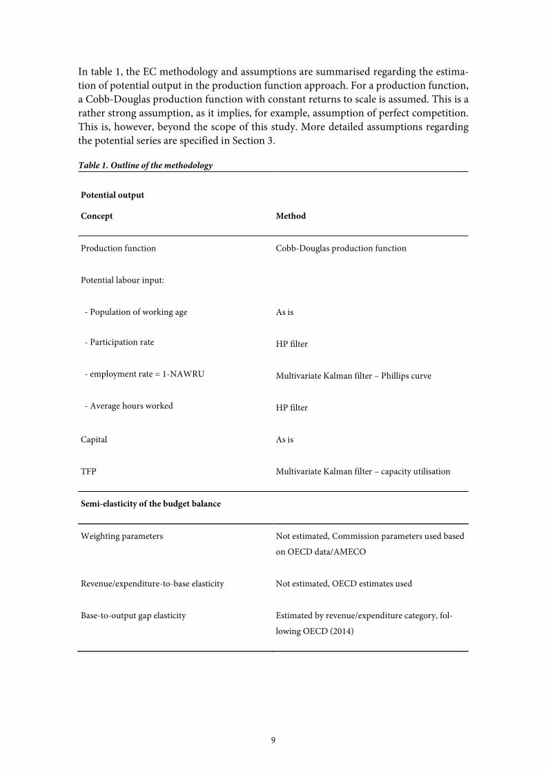
9

In table 1, the EC methodology and assumptions are summarised regarding the estima-tion of potential output in the production function approach. For a production function, a Cobb-Douglas production function with constant returns to scale is assumed. This is a rather strong assumption, as it implies, for example, assumption of perfect competition. This is, however, beyond the scope of this study. More detailed assumptions regarding the potential series are specified in Section 3.

Table 1. Outline of the methodology

Potential output

Concept Method

Production function Cobb-Douglas production function

Potential labour input:

- Population of working age As is

- Participation rate HP filter

- employment rate = 1-NAWRU Multivariate Kalman filter – Phillips curve

- Average hours worked HP filter

Capital As is

TFP Multivariate Kalman filter – capacity utilisation

Semi-elasticity of the budget balance

Weighting parameters Not estimated, Commission parameters used based

on OECD data/AMECO

Revenue/expenditure-to-base elasticity Not estimated, OECD estimates used

Base-to-output gap elasticity Estimated by revenue/expenditure category, fol-

lowing OECD (2014)

10

2.2 Budgetary semi-elasticity

In addition to considering the nominal general government revenue and expenditure to GDP and constructing an estimate for the output gap, the estimation of the cyclically ad-justed budget balance requires an estimate for the cyclical adjustment parameter, also called the budgetary semi-elasticity. It acts as a link between the cyclical position and the budget and corrects the budget balance for cyclical effects. In table 1, the principal com-ponents of the semi-elasticity are listed, as well as whether they are estimated in this paper or not.

More specifically, the semi-elasticity captures the absolute variation of the budget balance as a percentage of GDP to the relative variation of output gap. The budgetary semi-elas-ticity is multiplied by the output gap to determine the cyclical component of the budget, which is then subtracted from the actual balance-to-GDP ratio to yield the CAB. By using the semi-elasticity, the CAB is equal to the budget balance in a situation when production is at its potential level. (Mourre et al. 2013; Mourre et al. 2014.)

The calculation of budgetary semi-elasticity is characterised by a multi-step process in which the first step comprehends an estimation of the elasticity of various categories of government revenues or expenditures to the corresponding revenue or expenditure base. The second step is an estimation of the revenue or expenditure base to the output gap (details of this are presented in Section 3.5). To obtain the elasticity of overall budgetary revenue/expenditure to output gap, the individual elasticities obtained in the two steps are multiplied with each other within each revenue/expenditure category; these terms are then added together by using weighting parameters that take into consideration the share of each individual revenue/expenditure category to total general government revenue/ex-penditure. Finally, the budgetary semi-elasticity is obtained by adjusting the elasticity of revenue/expenditure-to-GDP ratio to the output gap with total revenues/expenditures-to-GDP ratio. (Girouard and André 2006; Mourre et al. 2014; Price et al. 2014.)

The Commission CAB methodology draws the data for the individual elasticities of ex-penditures and revenues to output gap from OECD calculations. These are used as a basis when calculating budgetary semi-elasticities. The budgetary semi-elasticity estimates are assumed time-invariant when computing the CAB, and the latest elasticity updates were completed in 2014.2 Similarly, the weighting parameters (the shares of the different reve-nue and expenditure categories of total revenues/expenditures and the ratio of expendi-tures/revenues-to-GDP) used in the computation of CAB were updated in 2013. These will be updated every six years, in line with every second update of Medium Term Objec-tives (MTO). (Mourre et al. 2014.)

The five individual revenue categories that are used in the estimation of the revenue elas-ticity of the budget are the personal income taxes, corporate income taxes, indirect taxes, social security contributions and non-tax revenue (see table 4 in Section 3.2 for details).

2 OECD further completed estimates for its own use in 2015 (Price et al. 2015).

11

For one cyclically sensitive spending category, namely unemployment-related expendi-ture, an elasticity estimate is obtained. For other expenditure categories, elasticities with respect to the output gap are assumed zero. (Mourre et al. 2014.)

2.3 Previous literature on the evaluation of the methodology

In general, estimation of the output gap is characterised by a high level of uncertainty, regardless of the estimation method. Uncertainty originates from several sources. First, data uncertainty affects estimates. This problem occurs for several reasons, such as the lack of the most recent data, revisions of published data and revisions in the projections. End-point uncertainty also arises, since the future path is unknown. The future cyclical development may also contain information about the current situation. Parameter esti-mation uncertainty is generated by the unobservable parameters estimated in each method. (Marcellino and Musso 2010; Murray 2014.)

The main criticism for the EU’s production function methodology has focused on its fail-ure in an upswing phase of cycles, like any mainstream output gap estimation method. However, the production function methodology outperforms the previous HP filter method and the IMF and OECD methods (Mc Morrow et al. 2015). Other weaknesses are related to the incorporation of the labour, capital and total factor productivity and the disregard for the open economy implications on output gaps (Darvas and Simon 2015).

The performance of the production function methodology has been evaluated and com-pared with the HP filter method. In the comparison, a revisions record was used as a per-formance measure and several criteria were considered. Short-term stability of the esti-mates was measured as a revision from one forecast to the next. When measuring the real-time reliability of the method, the real time and ex-post estimates were compared. The performance of the method during the financial crisis and the economic plausibility of the estimates was also evaluated. (Mc Morrow et al. 2015.)

According to this evaluation, the short-term stability of both methods was relatively good. The production function method has better real-time reliability than the HP filter method and it performs better in cyclical turning points. In addition, the production function method has improved since early years. The inclusion of hours worked and TFP has im-proved the method. However, the absolute performance of the EU methodology was poor during the pre-crisis period, 2006–2008. The revisions were five times greater before the financial crisis than after it. (Mc Morrow et al. 2015.)

Marcellino and Musso (2010) evaluated the reliability and forecasting performance of several output gap estimation methods. In contrast to previous evaluations, they con-cluded that no method was systematically superior to another method. However, this study was conducted in 2010 and the EU methodology has been modified since then. Murray (2014) also noticed that some methods are more likely to be revised than others and concluded that no estimation method is reliable at all times.

The production function methodology has received criticism for its deficient perfor-mance during economic booms. The use of financial information has been proposed as

12

one solution to determine whether output is at a sustainable level. Inflation is a signal of whether the output is above or below the potential level. However, the financial crisis showed that inflation might remain low and stable during a financial boom. Financial booms can coincide with positive supply shocks, which reduce inflation but increase asset prices. Economic expansion may increase labour supply by affecting both participation rate and immigration. Financial booms are also related to currency appreciation, which applies downward pressure on inflation. (Borio et al. 2013.)

Borio, Disyatat and Juselius (2013) propose an HP filter-based method to estimate fi-nance-neutral output gaps. Economic variables are added into the HP filter observation equation for output, and Kalman filter is used to calculate estimates for potential output. Credit and property prices are taken as proxies for the financial cycle. The relationship between the financial cycle proxies and output is assumed non-linear, since booms and busts are asymmetric. The estimated results show that the finance-neutral output gaps are robust compared to the standard HP filter approach and the OECD production function method. The performance is evaluated by comparing real-time and ex-post estimates. The finance neutral estimates are accurate for the United States, but for the United Kingdom and Spain they understate the boom.

Darvas and Simon (2015) propose an estimation method that integrates open economy characteristics by separating tradable and non-tradable sectors. According to the revi-sions of estimates, the proposed method performs better around the crisis years than the methods of the three institutions and the HP filter approach. In “normal” years, the an-nual revision of estimates is similar to the revisions of other estimates.

Bouis et al. (2012) have discussed the uncertainty of output gap estimates during the eco-nomic crisis. The recent crisis has decreased the level of potential output. Structural changes, such as high unemployment rate and low labour force participation, have shifted the potential output to lower level. Crises may also affect the equilibrium stock of capital and efficiency of its use. During the recent crisis, the actual output decreased significantly. In most countries, the widening output gap is due to the TFP gap.

Fioramanti et al. (2005) analyse sensitivity of output gap in relation to data revision, as-sumptions on the model and initial parameters of the estimation of NAWRU. Revisions to the output have been significant, and they are mostly due to potential labour and par-ticularly to the NAWRU.

3 Testing the components of the potential GDP

In the EC production function methodology, the estimation of potential output consists of several steps described in Section 3. In Section 3.1, the production function is intro-duced at a general level and some of its parameters are tested. The following section (3.2) deals with working age population, participation rate and average hours worked, which

13

are required in the estimation of potential labour. Section 3.3 concentrates on the estima-tion of NAWRU, also needed in the estimation of potential labour. In Section 3.4, as-sumptions behind the total factor productivity (TFP) are described and tested.

All data and baseline assumptions for the potential output calculations come from the EC autumn 2016 forecast. Data is available from the EC DG ECFIN CIRCABC Output Gaps library.3 Kalman filter estimations were done with the GAP program and its interfaces available from the library.

3.1 Production function parameters

The potential output is calculated using a production function and values for potential labour (L), capital (K) and total factor productivity (TFP). A production function is as-sumed to be a Cobb-Douglas production function with constant returns to scale:4

Y = LαK1-αTFP.

Output elasticities of labour (α) and capital (1-α) are not estimated. Instead, conventional mean values 0.65 and 0.35 are used. These correspond closely to the values derived from the mean wage share of the EU-15 countries. Same elasticities are used for all countries (Havik et al. 2014, 10).

The assumption of fixed elasticities for all countries can be criticised. However, the choice of elasticities does not appear to have much influence on output gap estimates. Produc-tion function parameters were tested by calculating output gap estimates with alternative parameters. We tested output elasticities of labour from 0.55 to 0.75 (and hence of capital from 0.45 to 0.25).

This wide range of production function parameters does not seem to have a significant impact on the estimated output gap (Table 2). The maximum of absolute difference from the EC output gap (α = 0.65) with α = 0.55 or 0.75 is 0.30 percentage points, while the mean of absolute values of the EC output gap is 2.18 percentage points. When “true” val-ues of parameters are likely to be quite close to those used by the EC, production function parameters do not seem to be a source of significant uncertainty based on the Finnish experience. For the sake of simplicity, the assumption of fixed parameters seems to be reasonable.

3 https://circabc.europa.eu/w/browse/671d465b-0752-4a2e-906c-a3effd2340ba

4 This is a rather strong assumption, as it implies, for example, an assumption of perfect competition. See also criticism of production function for the Finnish economy in Kuusi (2017).

14

Table 2. Summary statistics of output gap differences for tested production function pa-

rameters, percentage points.

elasticities of la-bour (α)

mean of dif-ference

mean of absolute difference

max of absolute difference

mean of absolute output gap

0.55 0.08 0.13 0.30 2.16

0.60 0.04 0.06 0.15 2.17

0.65 0.00 0.00 0.00 2.18

0.70 -0.04 0.06 0.15 2.19

0.75 -0.08 0.13 0.30 2.21

3.2 Working age population, participation rate and average hours worked

In the calculation of potential production, an estimate of potential labour input is a key variable. Labour input is measured as hours worked, and the potential hours worked is calculated from working age population, estimated potential participation rate, estimated potential unemployment rate (=NAWRU) and estimated potential average hours worked:

L = working age population x participation rate x (1-NAWRU) x average hours

worked.

The most critical component of the potential labour input, the estimate of NAWRU, non-accelerating wage rate of unemployment, and its impact are discussed in Section 3.3. This section deals with the working age population, the potential participation rate and the potential average hours worked. For the working age population, the actual working age population is used, as it has no cyclical component. For the other two, the potential is their trend obtained using HP-filter.

However, even if the working age population is not trended, the selection of the working-age population variable may influence the potential participation rate through its time series forecast. The trending of participation rate and average hours worked is done for variables extended with their forecasts up to t+8 years. A forecast up to t+2 is from the ECFIN forecast and after that a time series AR forecast is used.5

While uncertainty resulting from forecasts is not within the scope of this study, it is worth noting the possible implications from working-age population variable selection. The working-age population variable in the EC method is population aged 15–74, but unem-ployment rate is that of those aged 15–64. Thus, the participation rate used is not the

5 The forecast time series model specification is country specific. For Finland the participation rate model is AR(3) with

a constant and the average hours worked model is an AR(2) with a constant.

15

actual participation rate but one obtained using those population and unemployment rate variables.

That might have implications on the forecast of participation rate and thus on the poten-tial participation rate, as in Finland the number of people in age groups 15–74 and 15–64 have changed very differently in recent years. The number of 15–64 year olds has de-creased, while the number of 15–74 year olds is increasing. Thus, the actual participation rate for 15–74 and calculated participation rate used in the EC method have evolved dif-ferently (Figure 1) as well.

Figure 1. Participation rate in Finland: official for aged 15–74, rate used by the EC and

estimated potential participation rate by the EC. Source: EC DG ECFIN.

The potential participation rate and the potential average hours worked are their trends, obtained using the Hodrick–Prescott (HP) filter. The HP filter is a mathematical method that aims to remove the cyclical component of the time series so that the trend of the time series remains. Its first notable use was to find the trend of USA quarterly GDP data (Ho-drick and Prescott 1997). Since then, it has been widely used, especially in the real business cycle theory.

Using the HP-filter to estimate the trend presents problems. Firstly, the estimated trend does not necessarily correspond to the “right” trend, as it could introduce dynamics that are not present in the original series (Cogley and Nason 1995; Hamilton 2016). Secondly, the selection of the smoothing parameter, lambda, is not very well-grounded.

16

The lambda value used in HP filtering determines how much of the variability is ac-counted to a cyclical and to a trend component. However, the standardly used values are selected ad hoc. The lambda value used by Hodrick and Prescott (1997) was based on a reasoning of cycle and trend variances in the US GDP using quarterly data. They thought that assumptions of 5 % and 1/8 % for the variances of cycle and trend component, re-spectively, were appropriate. That gives a lambda of 1600, which has been commonly used for quarterly data thereafter. Even if the assumptions that Hodrick and Prescott made are appropriate for the US quarterly business cycles, there are, however, no reasons that those assumptions are appropriate for other applications (Harvey and Trimbur 2008).

As 1600 is usually used for quarterly data, there is more variability for annual data. It is shown that 6.25 for annual data equals that of 1600 for quarterly data (de Jong and Sa-karya 2016; Ravn and Uhlig 2002). However, probably the most commonly used lambda for annual data is 100, as suggested by Backus and Kehoe (1992). Also, 400 is used (Cooley and Ohanian 1991).

Nonetheless, HP filter is usually used to smooth volatile business cycle variables. A par-ticipation rate and an average hours worked series are smoother to begin with. Therefore, small lambda values give trends that are quite closely following the actual series. That is also the case with the EC’s potential participation rate and the average hours worked se-ries, as they are using the HP filter with a lambda value of 10 (Figure 2).

At least for Finland, the participation rate fluctuates with cycles, but the HP-filtered trend with lambda 10 tracks quite closely with the actual rate and fluctuates similarly. The fluc-tuation is mostly due to movement of groups like students in and out of labour market based on the labour market situation. Thus, it should not influence the potential partici-pation rate.

The proper potential participation rate should probably take into account demographics and social status of different groups in labour market. At least, it should not fluctuate as much as the original series. To more easily obtain a smoother trend than the EC’s trend, we ran the test using higher lambda values in order to smooth the participation rate and the average hours worked.

In addition to lambda = 10 used by the EC, we tested lambda = 100 and an even higher lambda = 1000. The 100 is quite commonly used in literature for annual data. The 1000 is a lot higher than that normally used for annual data. It was based on our judgment about how the trend of participation rate would probably look if cyclical component would be mostly removed. In our view, it produces a more convincing potential partici-pation rate than the EC’s potential participation rate (lambda = 10) or the rate with lambda = 100 (Figure 2). It is good to remember that more widely used lambda values do not have any theoretical foundation either.

We have calculated alternative participation rates for Finland and for comparison also for Germany, Spain and Sweden. Germany, and to a degree Sweden, differ from Finland and Spain, as they do not seem to have long cycles in the participation rate. Thus, the lambda choice does not have as considerable an influence as in Finland and Spain. Using a smoother trend of the participation rate as a potential participation rate has a substantial

17

influence on the output gap. In the case of Finland, the difference from the EC’s output gap can be up to two percentage points using the smoother trend (Figure 3).

Figure 2. Potential participation rate, actual and trend with lambda = 10, 100 and 1000,

%. Source: EC DG ECFIN and authors’ calculations.

18

Figure 3. Output gap difference from ECFIN estimation using potential participation

rate estimated with lambda = 100 and 1000. Source: EC DG ECFIN and authors’ calcu-

lations.

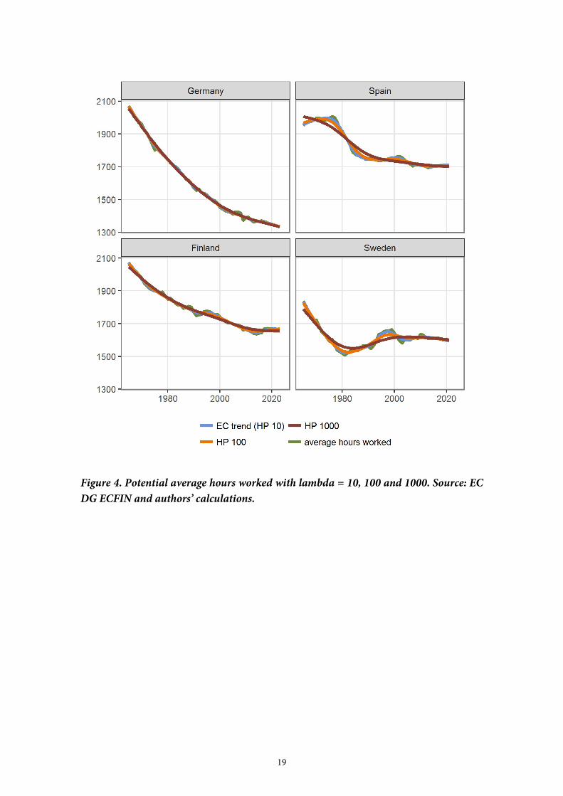
For average hours worked, the impact of lambda is much more moderate in Finland and Germany. This follows from the fact that the actual series fluctuates much less than the participation rate (Figure 4). In Finland, the fluctuation of average hours is almost as moderate as in a much larger country like Germany. Spain and Sweden have a much greater fluctuation.

Thus, the impact of lambda choice on the output gap is quite small in Finland and Ger-many (Figure 5). Maximum deviation of the output gap with lambda = 1000 for average hours from the EC output gap is approximately 0.7 percentage points and usually the deviation is less than 0.3 percentage points.

19

Figure 4. Potential average hours worked with lambda = 10, 100 and 1000. Source: EC

DG ECFIN and authors’ calculations.

20

Figure 5. Output gap difference from ECFIN estimation using average working hours

estimated with lambda = 100 and 1000. Source: EC DG ECFIN and authors’ calculati-

ons.

3.3 Unemployment rate

The most important variable when estimating the potential labour input is the estimation of the potential unemployment rate. In the EC method, the potential unemployment is the trend unemployment estimated using the multivariate Kalman filter. The Kalman fil-ter tries to incorporate information from time series models and the theory of Phillips-curve in form of NAWRU, the non-wage inflation accelerating rate of unemployment.

That is by no means the only way to estimate potential unemployment. Structural meth-ods such as DSGE models could also be used, but their implementation is more compli-cated and therefore are not very practical for the output gap estimation. Therefore, a “di-rect” method, which the EC method is considered, is a more natural choice.

A direct method can be univariate or multivariate. The univariate only uses information from the series itself. HP filter is an example of a univariate method. The EC method is a multivariate method as it combines information from the movement of the time series itself and its co-movement with another variable: for example, unemployment with real unit labour cost.

Within univariate and multivariate methods, actual models must be specified. In both univariate and multivariate methods, time series models to formulate movements of com-

21

ponents of time series is needed. In this case, time series models for trend and cycle com-ponents is included. In addition, in a multivariate method, one also has to model the co-movement of additional explanatory variables with the variable of interest.

In the EC method, only one additional explanatory variable is used, but there are two choices: real unit labour cost (in new Keynesian Phillips curve [NKP] model) and nominal unit labour cost (in traditional Keynesian Phillips curve [TKP] model). However, there could also be many others, such as various inflation measures, oil price, productivity and long term unemployment (see Logeay and Tober 2006). Furthermore, one has to decide about the actual model specification.

Estimation is also influenced by the estimation method and choices made in the estima-tion. For unemployment, the EC uses maximum likelihood (ML) estimation. For TFP, which is dealt with in Section 3.4, Bayesian estimation is used. Within ML estimation, choice of bounds for estimated parameters does have a considerable influence.

In addition, forecast issues have an impact on the estimation of potential unemployment (for sensitivity to forecast period, see Fioramanti 2016).

In this section, we evaluate the role of choice between a univariate and a multivariate model, the role of bounds for estimated parameters and the role of new anchoring technic. But first we introduce the NAWRU estimation in more detail (based on Havik et al. 2014; Planas and Rossi 2015).

3.3.1 Overview of potential unemployment rate estimation

The potential unemployment rate is the trend of unemployment rate. In the EC method, it is estimated using bivariate Kalman filter.

For the estimation of the trend unemployment rate, the unemployment rate is broken to a trend and a cycle component:

ut = u*t + (u-u*)t (=trend + cycle) (1)

Furthermore, the EC uses the Phillips curve relation between wage inflation and the cycle component of unemployment to estimate the cycle component. The idea is that the trend corresponds to NAWRU, the unemployment rate that describes the level of unemploy-ment that is consistent with steady wage inflation. Unemployment under that rate would lead real wages to rise faster than productivity.

22

So, in the NKP6 formulation used for Finland, the cycle component of unemployment rate is related to a change in the growth rate of real unit labour costs (RULC). The speci-fication is:

Δrulct = µπ + αΔrulct-1 – β0(u – u*)t +β1(u – u*)t-1 + art, (2)

where, µπ is the intercept, Δrulct is the change in the real unit labour costs and u – u* depicts the unemployment gap and art is an error term.7

In addition, the univariate part defines the time series models for trend and cycle compo-nents. Shocks to the trend unemployment are assumed to have a permanent effect and they reflect supply side shocks. Thus, the trend component is assumed to follow a second order random walk:

u*t = u*

t-1 + µt-1 + apt, where µt = µt-1 + aµt. (3)

Shocks to cyclical unemployment are assumed to have a temporary effect and they reflect demand side shocks. Thus, the cycle component is assumed to follow an AR(2) process:

(u-u*)t = φ1 (u-u*)t-1 + φ2 (u-u*)t-2 +act. (4)

The model specification and restrictions in estimation dictate how much of the variability of unemployment rate is allocated to cycle component and how much to the trend com-ponent. The more variability is allocated to the trend component, the more closely the trend unemployment rate follows the actual unemployment rate. In estimations of the EC the trend follows quite closely the actual unemployment rate. That is particularly a prob-lem for countries with large changes in unemployment, like those experienced in Finland or Spain, in contrast to countries like Germany and Sweden (Figure 6).

6 Currently, two specifications are used to estimate the cyclically adjusted unemployment rate: a traditional Keynesian

Phillips curve (TKP) and a new Keynesian Phillips curve (NKP). The NKP is preferred and used for Finland. NKP should be less pro-cyclical than TKP, especially when nominal wages react stronger than prices (Havik et al. 2014, 18). For Finland, a method change did not seem to have an effect, at least for the years 2013–2015 (Havik et al. 2014).

7 Also, the forward-looking restriction 𝛽 = 𝛽 𝜙 𝛿, 𝛿 = 0.97 is imposed; see Galí (2011).

23

Figure 6. Unemployment rate, actual, forecast and cyclically adjusted. Source: EC DG

ECFIN.

3.3.2 NAWRU model specification: Phillips curve

Inclusion of the Phillips curve to the model should improve estimation of the trend and make it less sensitive to cyclical fluctuations. The idea is that if the employment situation worsens, unemployment rises and wage growth slows down at the same time. Thus, the cyclical component of unemployment rate rises, not the trend component.

However, there is a lot of criticism against the Phillips curve concept in general. The NAIRU concept does not seem to hold empirically (Farmer 2013). Or, at least, the relation is looser than before (R. Arnold 2008). Not everyone, however, agrees with the criticism (Gordon 2013). Still, even if the Phillips curve is still alive, as inflation expectations have become anchored the unemployment is more related to the level of inflation than the rate of change (Blanchard 2016). Also, the coefficient between inflation and unemployment is small, and the fit of the relation is relatively poor (Blanchard et al. 2015). Troubling for

24

Finland, the Phillips curve is a more relevant concept in a large closed economy than in small open economies (Fabiani and Mestre 2000).

As the Phillips curve seems to be at least empirically on weak ground, we assessed esti-mating NAWRU for Finland without the Phillips curve. Otherwise, the model and the parameter restrictions were the same. In practice, and in line with the criticism, the Phil-lips curve does not seem to have that significant a role in estimating the trend unemploy-ment, at least in Finland. Removal of the Phillips curve from the estimation does not sig-nificantly change the trend unemployment (Figure 7).

This is in line with results from Gechert et al. (2014) that the EC’s estimate of NAWRU is largely driven by actual unemployment rather than the RULC via the Phillips curve. In effect, that means that EC’s method is largely that of a univariate, rather than a multivar-iate. It could be, however, that the Phillips curve has predictive power in the cycle turning points, and its inclusion is justified on that ground.

Figure 7. Unemployment rate and trend unemployment rate with and without Phillips

curve, %. Source: EC DG ECFIN and authors’ calculations.

To improve the Phillips relation one might consider to model it as a level Phillips curve (Blanchard et al. 2015), use the long term unemployment rate (Rusticelli 2014) or include the age structure of the labour force (Dixon et al. 2016).

25

3.3.3 NAWRU model specification: cycle and trend state equations and their estimation

As the Phillips curve has limited influence on potential employment rate, state equations for cycle and trend components of the unemployment rate largely determine how and how much the potential unemployment is evolving in time.

Assumptions made regarding the state equations include a specification of state equations for cycle and trend components as they are presented in equations 3 and 4. In the estima-tion, assumptions are also made regarding bounds to estimated parameters and to esti-mated innovation variances.

Not all restrictions regarding bounds are equally important. In practice, bounds for inno-vation variances (error variances) of trend and cycle equations are most important. Esti-mated trend and cycle components of unemployment depend significantly on restrictions imposed on the trend, slope and cycle innovation variance. Error variances of state equa-tions determine how much variance of the variable is allocated to a trend and how much to a cycle component. Trend and slope innovation variances determine together how much variance is allocated to the trend.

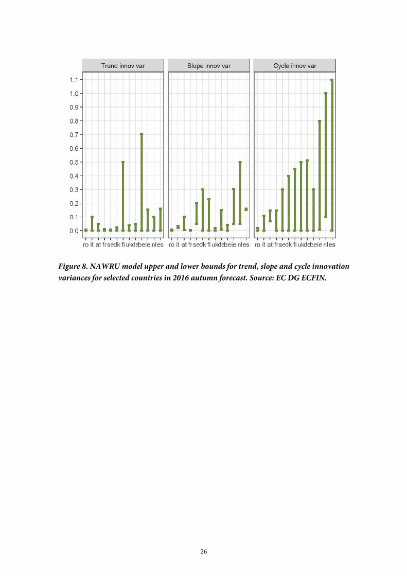
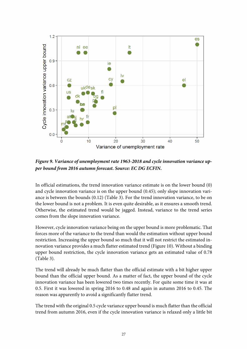
For Finland, the trend innovation variance is restricted to a range 0–0.50, slope variance to a range 0–0.23, and the cycle innovation variances is restricted to a range 0–0.45 by the EC. The cycle variance bounds for Finland are close to the average among the EU coun-tries (Figure 8). There is, however, a wide range of cycle upper bounds, from 0.02 for Romania to 1.1 for Spain. Cycle upper bounds are correlated with the variance of unem-ployment. The trend and the slope variance upper bounds for Finland are among the highest in the EU.

In theory, it would be reasonable to assume that the variance of cycle component is larger than the trend component. Upper bounds set for Finland do not imply this. However, in practice, bounds do not necessarily restrict estimated parameters. Indeed, with the cur-rent cycle upper bound the trend and slope variance upper bound do not have an effect in practice, as the estimated trend variance is on the lower bound and the slope variance between bounds.

26

Figure 8. NAWRU model upper and lower bounds for trend, slope and cycle innovation

variances for selected countries in 2016 autumn forecast. Source: EC DG ECFIN.

27

Figure 9. Variance of unemployment rate 1963-2018 and cycle innovation variance up-

per bound from 2016 autumn forecast. Source: EC DG ECFIN.

In official estimations, the trend innovation variance estimate is on the lower bound (0) and cycle innovation variance is on the upper bound (0.45); only slope innovation vari-ance is between the bounds (0.12) (Table 3). For the trend innovation variance, to be on the lower bound is not a problem. It is even quite desirable, as it ensures a smooth trend. Otherwise, the estimated trend would be jagged. Instead, variance to the trend series comes from the slope innovation variance.

However, cycle innovation variance being on the upper bound is more problematic. That forces more of the variance to the trend than would the estimation without upper bound restriction. Increasing the upper bound so much that it will not restrict the estimated in-novation variance provides a much flatter estimated trend (Figure 10). Without a binding upper bound restriction, the cycle innovation variance gets an estimated value of 0.78 (Table 3).

The trend will already be much flatter than the official estimate with a bit higher upper bound than the official upper bound. As a matter of fact, the upper bound of the cycle innovation variance has been lowered two times recently. For quite some time it was at 0.5. First it was lowered in spring 2016 to 0.48 and again in autumn 2016 to 0.45. The reason was apparently to avoid a significantly flatter trend.

The trend with the original 0.5 cycle variance upper bound is much flatter than the official trend from autumn 2016, even if the cycle innovation variance is relaxed only a little bit

28

(Figure 10). Thus, unemployment rate trend estimation is very sensitive to the cycle in-novation upper bound. That has also been reported previously, at least by Fioramanti (2016) for Italy and Kuusi (2017) for Finland.

Figure 10. Unemployment rate, an official EC trend unemployment rate, and alterna-

tive trends with no upper bound and with 0.5 upper bound restriction for cycle innova-

tion, %. Source: EC DG ECFIN and authors’ calculations.

This is problematic, as those bound values do not have any clear justification. The EC have responded to the bound criticism, arguing that estimation without restrictions may lead to a constant or a deterministic trend for the NAWRU and a non-stationary cycle (Hristov and Roeger 2017). That is a reasonable argument, and we agree that the trend estimated without an upper bound on the cycle innovation variance is probably too flat. Without an upper bound on the cycle, the slope innovation variance is in fact only 0.002, while the trend innovation variance is zero on the lower bound.

That is not, however, justification for the current bound values. There are other bound combinations that produce NAWRU series, which differs from the EC series but meets the criteria set in (Hristov and Roeger 2017). It could, for example, be more compelling to limit the slope innovation variance from below than the cycle from above. That is al-ready done for some EU countries (see Figure 8). We have also tested that alternative with various lower bounds.

29

To test the influence of NAWRU estimation modifications, we have tested several alter-natives. We have varied the cycle innovation upper bound and the slope innovation lower bound and tested the model without the Phillips curve. The properties of estimated mod-els and estimates for innovation variances are reported in Virhe. Kirjanmerkille ei ole annettu nimeä.. Alternatives produce mostly flatter trend series than the official (Figure 11).

Table 3. Estimated NAWRU alternatives.

Bounds Estimated

Phillips-curve trend slope cycle trend slope cycle

official x LB 0 - UB 0.45 0 0.120 0.45

no_upper x LB 0 - - 0 0.002 0.781

slope_lb0_1 x LB 0 LB 0.1 - 0 0.1 0.633

slope_lb0_2 x LB 0 LB 0.2 - 0 0.2 0.536

slope_lb0_005 x LB 0 LB 0.005 - 0 0.005 0.767

slope_lb0_05 x LB 0 LB 0.05 - 0 0.05 0.691

slope_lb0_01 x LB 0 LB 0.01 - 0 0.01 0.752

cycle_ub0_4 x LB 0 - UB 0.40 0 0.189 0.4

cycle_ub0_5 x - - UB 0.50 0.046 0.006 0.5

nophillips - LB 0 - UB 0.45 0 0.182 0.45

nophillips_no_upper - LB 0 - - 0 0.005 0.770

30

Figure 11. Unemployment rate and alternative trend unemployment rates, %. Source:

EC DG ECFIN and authors’ calculations.

3.3.4 Forecast with anchoring

NAWRU estimation is done using unemployment rate data up to year t+2 with a forecast from the EC. In addition, since the 2016 autumn forecast the new method to “anchor” unemployment is used (European Commission 2016, 68). The anchoring uses the struc-tural unemployment rate from the EC’s T+10 calculation.8 That means that the NAWRU is estimated so that it will equal structural unemployment rate at year t+10.9

For Finland, the anchor rate is 7.564159, with an eight-year horizon (8 + 2 for EC forecast = 10). The anchoring does influence the NAWRU for the last ten years (Figure 12).

8 For structural unemployment rate, see (Orlandi 2012).

9 We haven’t found the description of the methodology.

31

Figure 12. Difference from NAWRU without anchoring. Source: EC DG ECFIN and au-

thors’ calculations.

Even if the NAWRU estimation with anchoring gives the series up to t+10, the series is used for the output gap calculation only up to year t+2. Years up to t+5, required for the output gap, are filled with the constant technical forecast: the last value plus half of the last change.10

3.3.5 Mean-adjustment of NAWRU

The estimated NAWRU is “mean-adjusted” for countries for which NKP is used in the estimation. The rationale for mean-adjustment is to make results from NKP and TKP comparable. In practice, if a mean of NAWRU from NKP is higher than that from TKP, the NKP NAWRU is adjusted downward. (Havik et al. 2014, 23.)

The mean-adjustment is, however, quite dubious. There are no theoretical arguments for the practice. The adjustment is not symmetric. It is done only if the mean of NKP-NA-WRU is higher. The adjustment is not done based on an actual difference but on a fixed

10 NAWRU(t+[3-5]) = NAWRU(t+2) + 0.5*( NAWRU(t+2) - NAWRU(t+1)).

-1,0

-0,8

-0,6

-0,4

-0,2

0,0

0,2

0,4

1995 2000 2005 2010 2015

Anchored Anchored, horizon = 4

Anchored, trend anchor = 5 Anchored, trend anchor = 5, horizon = 4

32

difference from the spring 2014 forecast. There are no reasons the differences should re-main constant.

The adjustment factor for Finland is one of the highest, -0.72. Only Sweden (-0.94) and Greece (-0.92) have higher factors. Factor means that the trend unemployment rate used in the output gap calculations is 0.72 percentage points lower than the actual estimated trend unemployment. This translates to about a 0.5 % higher potential GDP and a 0.3 percentage point higher cyclically-adjusted budget balance.

3.4 TFP

In addition to potential labour input, the potential total factor productivity (TFP) is the second component that determines the potential production, as the potential capital input is the capital as it is. The potential TFP is the trend of the TFP estimated using a multi-variate Kalman filter, as is the trend unemployment rate. Discussion in the beginning of Section 3.3 also applies mainly to the TFP estimation. However, the potential TFP is esti-mated using Bayesian estimation, whereas the unemployment rate is estimated with max-imum likelihood. So, instead of parameter restrictions, setting of parameters for prior dis-tributions is one of the choices in modelling that influences the estimation of the potential TFP.

Another variable used for the detrending of TFP is capacity utilisation, because it is thought that it co-moves with the unobservable cyclical component of TFP. The variable for capacity utilisation is a composite constructed by the EC (see Havik et al. 2014, 65).

In the Kalman filter model in log form, the TFP is broken down into trend and cycle components:11

𝑡𝑓𝑝 = 𝑝 + 𝑐 , (=trend + cycle), (5)

and the change of capacity utilisation is related to a cycle component of the TFP:

𝑢 = 𝜇 + 𝛽𝑐 + 𝑒 , (6)

where μ is constant, β is a coefficient of link between TFP-cycle and capacity utilisation. Its theoretical value is determined by a correlation between labour and capital capacity utilisation and the labour share of income and should be greater than one (see Planas et al. 2010). The eUt is an error term. For most countries, the error is assumed to be a white noise random shock. For Finland, France and Slovenia, it is an AR(1) random shock:

𝑒 = 𝛿 𝑒 + 𝑎 , (7)

where AR-coefficient have an absolute value less than 1 and 𝑎 is a white noise random shock.

11 A description of the model is based on (Havik et al. 2014; Planas et al. 2010; Planas and Rossi 2015).

33

Dynamics of variables in the transition equations are modelled with time series models. The trend is assumed to follow a damped trend model:

𝑝 = 𝑝 + 𝜇 and

𝜇 = 𝜔(1 − 𝜌) + 𝜌𝜇 + 𝑎 , (8)

where ω represents an average growth rate of the TFP and 𝜌 is the persistence of the slope of the trend and 𝑎 is an error term.

The TFP cycle is assumed to follow an AR(2) process with complex roots:

𝑐 = 2𝐴𝑐𝑜𝑠 𝑐 − 𝐴 𝑐 + 𝑎 , (9)

where A is an amplitude, τ a periodicity of the cycle and act is an error term. This cycle formulation is assumed because it allows inserting prior information about the business cycle (Planas and Rossi 2015, 19).

For Finland, the model is estimated from 1980. For the years before that, apparently, the HP filter is used. Use of Bayesian estimation means that all parameters are assigned a probability distribution before estimation. Priors can be set based on prior knowledge or from prior estimation. In the EC’s GAP-programme, estimated priors can also be set us-ing parameters from ML estimation.

In the following section, assumptions in estimation we have found to be central are tested. We considered assumptions regarding TFP trend and cycle models and their prior distri-butions. Also, the assumption of bivariate model in form of inclusion of capacity utilisa-tion indicator is considered.

3.4.1 TFP trend assumptions

The trend of TFP is assumed to follow a damped trend model that includes an estimated mean growth rate and a persistence of the slope. Modelling assumptions here are the model formula and priors for mean growth, persistence and error variance. Error vari-ances of trend and cycle determine how much variance of TFP is allocated to the trend and the cycle. The lower the proportion of the trend of the error variance, the smoother the potential TFP series will be.

A prior for mean TFP growth rate (ω) is 1.5 %, and a prior for the persistence of the slope of the trend (ρ) has a mean of 0.8, meaning 80 % of slope parameter comes from the lagged slope value and 20 % from the mean growth rate. (Table 4.)

The set prior for mean growth is between observed mean from 1965, 1.9 %, and the one from 1980 (estimation period), 1.3 %. It is somewhat higher than the mean growth of posterior distribution (1.3 %) and the one for ML estimation (0.8 %). However, tweaking the prior mean of mean growth by setting it from 1 % to 2 % does not have a noticeable effect.

34

Table 4. Priors for trend set by the EC (and priors from maximum likelihood).

mean variance range

ω 0.015 (0.0084) 0.01003 (0.0088) 0 – 0.03

ρ 0.8008 (0.9887) 0.2375 (0.0128) 0 – 0.99

Vµ 4.7e-6 (2e-6) 4.7e-6 (2e-6)

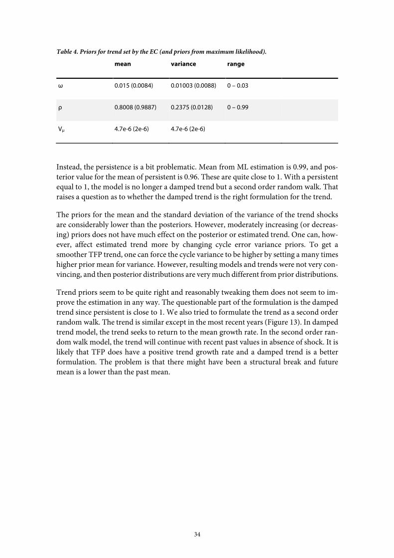
Instead, the persistence is a bit problematic. Mean from ML estimation is 0.99, and pos-terior value for the mean of persistent is 0.96. These are quite close to 1. With a persistent equal to 1, the model is no longer a damped trend but a second order random walk. That raises a question as to whether the damped trend is the right formulation for the trend.

The priors for the mean and the standard deviation of the variance of the trend shocks are considerably lower than the posteriors. However, moderately increasing (or decreas-ing) priors does not have much effect on the posterior or estimated trend. One can, how-ever, affect estimated trend more by changing cycle error variance priors. To get a smoother TFP trend, one can force the cycle variance to be higher by setting a many times higher prior mean for variance. However, resulting models and trends were not very con-vincing, and then posterior distributions are very much different from prior distributions.

Trend priors seem to be quite right and reasonably tweaking them does not seem to im-prove the estimation in any way. The questionable part of the formulation is the damped trend since persistent is close to 1. We also tried to formulate the trend as a second order random walk. The trend is similar except in the most recent years (Figure 13). In damped trend model, the trend seeks to return to the mean growth rate. In the second order ran-dom walk model, the trend will continue with recent past values in absence of shock. It is likely that TFP does have a positive trend growth rate and a damped trend is a better formulation. The problem is that there might have been a structural break and future mean is a lower than the past mean.

35

Figure 13. TFP growth, trend with damped trend and second order random walk.

Source: EC DG ECFIN and authors’ calculations.

3.4.2 TFP cycle assumption in transition equation

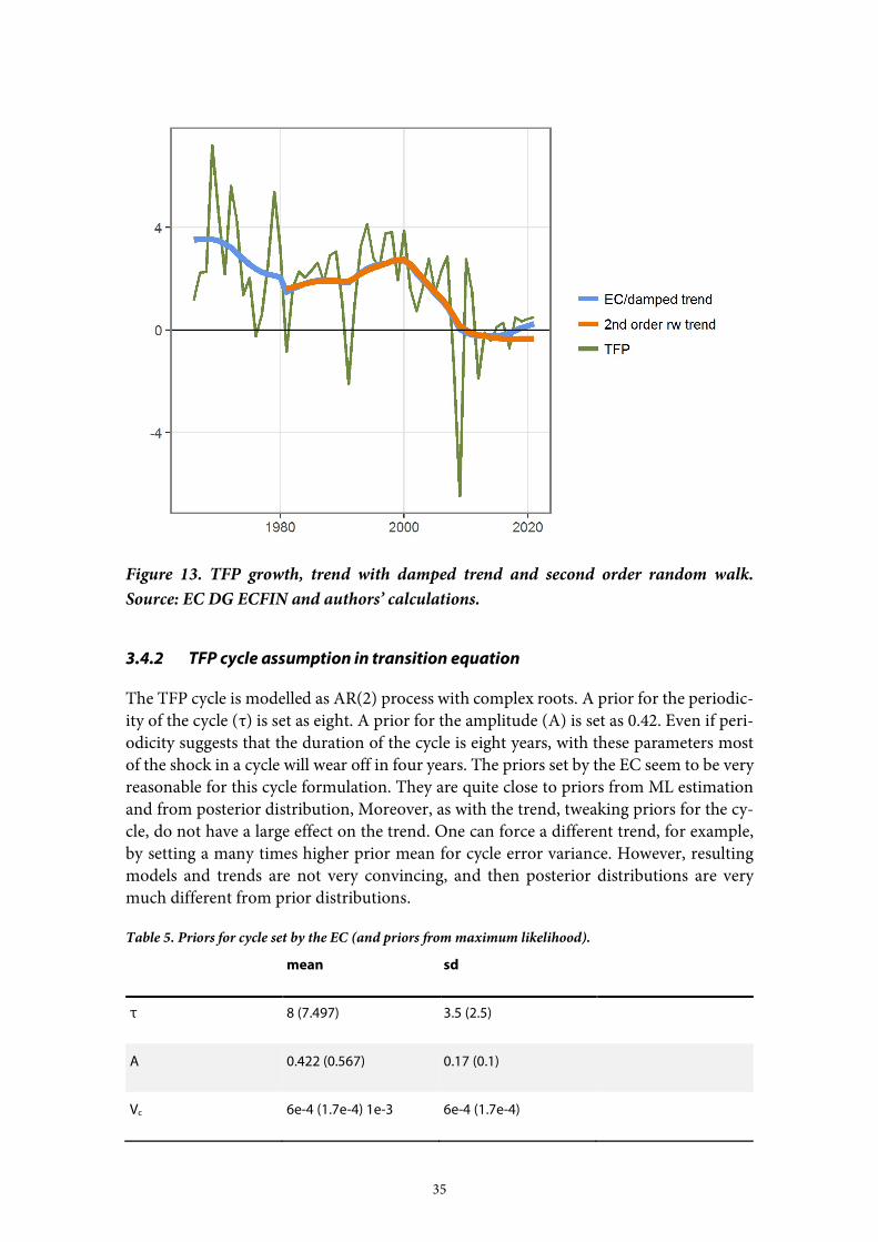
The TFP cycle is modelled as AR(2) process with complex roots. A prior for the periodic-ity of the cycle (τ) is set as eight. A prior for the amplitude (A) is set as 0.42. Even if peri-odicity suggests that the duration of the cycle is eight years, with these parameters most of the shock in a cycle will wear off in four years. The priors set by the EC seem to be very reasonable for this cycle formulation. They are quite close to priors from ML estimation and from posterior distribution, Moreover, as with the trend, tweaking priors for the cy-cle, do not have a large effect on the trend. One can force a different trend, for example, by setting a many times higher prior mean for cycle error variance. However, resulting models and trends are not very convincing, and then posterior distributions are very much different from prior distributions.

Table 5. Priors for cycle set by the EC (and priors from maximum likelihood).

mean sd

τ 8 (7.497) 3.5 (2.5)

A 0.422 (0.567) 0.17 (0.1)

Vc 6e-4 (1.7e-4) 1e-3 6e-4 (1.7e-4)

36

3.4.3 TFP second measurement equation – a capacity utilisation indicator

For the estimation of TFP, capacity utilisation is measured using combined capacity uti-lisation indicator based on:

– capacity utilisation in industry

– economic sentiment indicator for the services sector and

– economic sentiment indicator for the construction sector

Individual capacity utilisation indicators are rescaled so that the variance of the indicator corresponds to the variance of the estimated value added cycle of the sector in question. The combined indicator is a weighted average of individual indicators. Weights are shares of corresponding sectors in the total economy. Shares are based on HP filtered value added trends. (Havik et al. 2014, 65).

For Finland, the combined capacity utilisation indicator starts from 1996, as the economic sentiment indicator for the services sector starts from that year. Planas et al. (2010) have tested the capacity utilisation for manufacturing and the EC Business Survey indicator.

Omitting a capacity utilisation indicator and thus the second measurement equation from the model altogether does not significantly change results for Finland except in the cycle turning points (Figure 14). So, in the case of TFP, as in the case of NAWRU, the trend is primarily a result of the univariate time series smoothing, and the variable from the sec-ond equation does not have a significant effect.

Table 6. Priors for capacity utilisation equation set by the EC (and priors from maximum likelihood).

mean sd

μU 0.0004 (-0.008) 0.032 (0.014)

β 1.4 (2.842) 0.705 (0.184)

δU 0.008 (0.454) 0.399 (0.121)

Vπ 2.5e-3 (1.5e-4) 2.5e-3 (1.5e-4)

37

Figure 14. Trend TFP with and without a capacity utilisation indicator, growth rate, %.

Source: EC DG ECFIN and authors’ calculations.

3.4.4 Tests for TFP

Overall, priors set for potential TFP estimation seem to be reasonable and tweaking priors does not seem to have a large effect on the estimated trend TFP. The largest effects come, as in the case of NAWRU, from the trend and cycle variances. We assessed several alter-native priors for trend and cycle parameters and also tested the trend modelled as AR(2). Alternative trend series do not deviate greatly from the EC baseline trend, except in the most recent years (Figure 15).

Selected for testing are:

– Priors from maximum likelihood estimation

– Trend modelled as second order random walk, official priors

– Priors from posterior distribution

– Significantly higher priors set for cycle variance and lower for trend compared to the

official

38

Figure 15. TFP, EC baseline trend and alternative trend growth rates. Source: EC DG

ECFIN and authors’ calculations.

4 Semi-elasticity of the budget balance

The EC calculations of the CAB require an estimate for the budgetary semi-elasticity in addition to the output gap estimates (see sections 2.1 and 2.2 for the description of the methodology and definitions). In Section 4.1, the estimation of individual elasticities of revenue and expenditure bases to output gap is described. How to construct the budgetary semi-elasticity from its building blocks is discussed in Section 4.2.

4.1 Individual base-to-output gap elasticities

The budgetary semi-elasticities are considered constant in the Commission estimates of the CAB (Mourre et al. 2014). However, it is important to grasp the idea of how semi-elasticities are affected by different output gap estimates, and how changes in the OG are linked to the CAB. These results are presented in Section 5.

In table 4 below, the five individual revenue categories that are used in the estimation of the budget’s revenue elasticity are listed, as well as one cyclically sensitive spending cate-gory, namely the unemployment-related spending. Also listed are the assumptions made about the elasticities and whether they are actually estimated or not for each country by the OECD (Price et al. 2014).

39

To obtain the budgetary semi-elasticity, estimates for the budget’s overall revenue and expenditure elasticities (ηR and ηG respectively in formula (11) below) are required. These are composed of revenue and expenditure elasticities to output gap of individual revenue and expenditure categories (ηRi,i and ηGU), weighted by the share of revenues and expend-itures of total revenues and expenditures, respectively (Ri/R and Gu/G). It is worth noting that each individual elasticity represented in formula (11), ηRi,i and ηGU, is a product of two elasticities, one representing revenue/expenditure-to-base, the other base-to-output gap, as seen in the middle and right-hand-side columns of Table 4. (Mourre et al. 2014.)

𝜀 = 𝜀 − 𝜀 = (𝜂 − 1)𝑅

𝑌− (𝜂 − 1)

𝐺

𝑌

= (∑ 𝜂 , − 1) − (𝜂 − 1) (10)

In this paper, we estimate only base-to-output gap elasticities to understand the impact of different output gap estimates on the budgetary semi-elasticity and finally on the CAB. The revenue/expenditure-to-base elasticities are assumed to follow the OECD (2014) es-timates. The revenue/expenditure-to-base elasticities are not estimated, since the OG es-timates computed in this paper do not affect them directly. Also, the revenue and ex-penditure shares are assumed unchanged from the Commission methodology, first tier of revisions (Mourre et al. 2013).

Table 4: Elasticity components used in the computation of the budgetary semi-elasticity (Mourre et al.

2014).

Revenue/expendi-

ture category Revenue/expenditure-to-base Base-to-output gap

Personal income

tax

Estimated: separately for different reve-

nue classes

Estimated, base: wages and salaries,

self-employment income and capital

income

Corporate income

tax Estimated

Estimated, base: gross operating sur-

plus

Indirect tax

1.0 by assumption (also estimated, but

no significant difference from unitary

elasticity)

1.0 by assumption

Social security con-

tribution

Estimated: separately for employer and

employee contributions Estimated, base: wages and salaries

Unemployment re-

lated expenditure 1.0 by assumption Estimated, base: unemployment

In the OECD estimates for the Commission, the base-to-output gap elasticities are calcu-lated using data that spans the period 1990–2013 (Mourre et al. 2014). The unemploy-ment related expenditure-to-base estimate contains data only until 2010, and the tax code 2010–2011 was used in the revenue-to-base estimates (Mourre et al. 2014). Computing

40

the expenditure/revenue-to-base requires complex simulations using detailed tax codes and micro-level income data for personal income tax and social security contributions, but estimating base-to-output gap is simpler (Price et al. 2014).12

When estimating the base-to-output gap elasticities in this paper, the same period of data (1990–2013) is analysed, but if available the latest revisions of data are used to evaluate the sensitivity of elasticity estimates to data revisions. The data sources are listed in Table A.1 in the appendix of this paper.

The base-to-output gap elasticity estimation for each base is specified in the first differ-ence form by using the following general construction (10), where coefficient α1 is inter-preted as a short-run elasticity, β as a long-run elasticity and λ depicts the error correction term (Price et al. 2014):

∆𝑙𝑛(𝑏𝑎𝑠𝑒 /𝑌 ) = 𝛼 + 𝛼 ∆𝑙𝑛(𝑌 /𝑌 ) + 𝜆(𝑙𝑛 − 𝛽𝑙𝑛 ) + 𝑢 (11)

OECD tests the model, where base refers to some tax base and Y and Yp to output and potential output, respectively, with three different specifications that are: 1) GLS cor-rected for AR(1) autocorrelation in residuals, 2) error-correction model and 3) a combi-nation of both (Price et al. 2014).13 The tax-base-to-output gap models are specified in first difference form in order to remedy the non-stationarity problems associated with the series. As it can be observed in (10), the revenue bases are normalised with the potential output. The unemployment rate is normalised using the NAWRU.

For each individual base-to-output gap elasticity estimate, used in the computation of each country’s budgetary semi-elasticity, the best specification is chosen in the OECD methodology (Price et al. 2014). In other words, the statistical significance of the error correction term (λ) dictates whether a specification including error-correction is chosen. R2 and the standard error are also defining factors when selecting the specification.

The results of the OECD estimation of individual elasticities, as well as our own estimates of them for different values of output gaps are shown in the appendix, Tables A.2 and A.3. In tables A.2 and A.3, the individual elasticities are calculated for the own estimates of the output gap (numbered 1–5) using only the specification that the European Commission uses in their own calculations, namely either the ECM or the ECM corrected for AR(1), depending on the revenue or expenditure class.14 The first own estimate, using the Com-mission estimate of the output gap and the latest revisions of data, is run using all the

12 In the Commission estimates, OECD data for the years 1990–2013 is retrieved from the OECD Economic Outlook

No. 93, No. 95, OECD Analytical Database and AMECO. ESA1995 data was used, but only marginal changes to the elasticity of base-to-output gap estimates would result from the use of ESA2010 data (Mourre et al. 2014).

13 In the specifications with no error correction term, the model takes the form: ∆ln(base /Y ) = α +α ∆ln(Y /Y ) + 𝑢

14 ECM i.e., specification [2] for gross operating surplus and capital income, ECM + AR(1) i.e., [3] for wages and salaries and unemployment.

41

three specifications in order to test the model and see if the specification selected by the Commission is the best when also using the most recent data revisions.

4.2 From individual elasticities to the semi-elasticity

All in all, when the output gap is estimated with changed parameter values, the base-to-output gap elasticities are likely to change. This affects the value of budgetary semi-elas-ticity as well; other components of the budgetary semi-elasticity remaining constant. The constancy of the other components is justified by the Commission methodology in which the weights of the budgetary items are updated only every six years. On the other hand, the revenue/expenditure-to-base elasticities utilise the 2010-2011 tax code data and could be updated to include the most recent data. However, as we aim at evaluating the effects of changes in the output gap on the CAB, the determination of these is not necessary for this end.

In the latest revision for the weighting parameters, an average over the 2002–2011 period was chosen. The weighting parameters are updated only every six years and, conse-quently, the same weighting parameters are used in this study. Therefore, the changes in the budgetary semi elasticity parameters come from changes in the individual elasticities calculated and, more specifically, the base-to-output gap elasticity.

Finally, the budgetary semi-elasticity can be obtained following the formula (11) in Sec-tion 4.1 (Mourre et al. 2014). There the elasticities of each individual revenue or expendi-ture base in relation to output gap (ηRi,i and ηGu) are weighted using the respective expendi-ture and revenue shares of the budget. Then individual elasticities (minus one) are mul-tiplied by corresponding expenditure and revenue shares of total GDP. Additionally, the weighted elasticities for gross operating surplus, wages and salaries and self-employment income are set to sum-up to 1; hence, the above-mentioned components are weighted by their corresponding income shares. (Price et al. 2014)

The semi-elasticities are presented in table 6 below and in table A.4.15 The semi-elasticities for revenue (εR), expenditure (εG) and budget balance (ε) are listed. In the estimates labelled EC OUTPUT GAP and 1–5, the data comes mainly from the OECD Economic Outlook 100/AMECO Autumn 2016. The impact of varying budgetary semi-elasticities on cyclically adjusted budget balance is discussed in Section 5.

The individual elasticity for wages and salaries is the main component explaining the de-viations of the estimates of budgetary semi-elasticity from the benchmark OECD estimate (see appendix table A.2). Our own estimate for this is significantly smaller (0.4–0.53) than the OECD estimate of 0.77. This result would suggest that the personal income tax reve-nues and social security contributions do not decrease in economic downturns as greatly as the OECD estimates would predict. Therefore, our own estimates of revenue elasticities and total budgetary semi-elasticities are consistently smaller than in the OECD estimate (0.49–0.52 vs. 0.57). This result might be due to use of a different data revision. However, the overall revenue elasticities are still close to zero (Table 6). The expenditure-to-base

15 Details of the assumptions made can be found in the appendix (Table A.4).

42

semi-elasticity, namely the elasticity of unemployment to output gap, is only slightly less negative in our own estimates than in the OECD benchmark (-0.58–-0.60 vs -0.6). This would imply that the unemployment expenditure is slightly less cyclical than the OECD estimates suggest.

In the estimate labelled EC OUTPUT GAP, the European Commission estimate of po-tential output and output gap (Autumn 2016) is used, and the output gap is the same as in the OECD benchmark case. This exhibits greatest variance among the potential outputs considered, in (5) the variance of potential output is the smallest. The variance of potential output in the remaining four series (1–4) falls between these two. Additionally, the vari-ance of NAWRU affects the semi-elasticity of expenditure-to-output gap through NA-WRU normalised unemployment rate.

Table 7. The semi-elasticities of revenue, expenditure and total budget balance for different output gaps.

SEMI ELASTICITY FOR:

Revenue (εR) Expenditure (εG) Budget balance (ε)

BENCHMARK, OECD

(2014) -0.031 -0.604 0.57304

EC OUTPUT GAP -0.077 -0.583 0.50599

(1) -0.078 -0.586 0.50869

(2) -0.089 -0.593 0.50395

(3) -0.083 -0.582 0.49881

(4) -0.083 -0.599 0.51585

(5) -0.099 -0.589 0.49045

When calculating base-to-output gap elasticities, there are some data issues that need to be considered. The availability of data, as well as the sensitivity of the estimation process to the time frame and reforms, could affect the elasticity estimates. The latter issue is es-pecially related to the revenue-to-base elasticity (Havik et al. 2014). On the other hand, in addition to modelling of AR(1) and error correction processes, further alternatives could be considered.

The effect of variation in the budgetary semi-elasticity estimates on the CAB is discussed in Section 5.2.

43

5 Computing the cyclically-adjusted budget balance

The cyclically-adjusted budget balance (CAB) is calculated as the difference between the nominal budget balance and the cyclical component. The cyclical component is calculated as a product of the OG and the budgetary semi-elasticity. To assess the impact of the out-put gap estimation on the CAB, we have estimated alternative output gap series based on alternative assumptions within the EC production function methodology. Alternative se-ries of components for the production function were described in Section 3. We have computed output gaps for all combinations of the alternative series. There were, including the EC baseline series, three alternatives for both the potential participation rate and po-tential average hours worked, eleven for potential unemployment rate and five for poten-tial TFP. Altogether there were 495 unique combinations.

5.1 Output gap

The variation in the trend estimates of the different components of the potential output is reflected in the outcomes when computing the output gap. The variation in the output gap estimates depending on the different trend estimates of TFP, NAWRU, participation rate and average hours worked can be seen especially during the troughs and peaks or after the direction of the cycle changes (Figure 17).

The largest variation from the EC baseline estimate can be detected at the beginning of the 1980s and mid-1990s. At the beginning of the 1980s, most alternatives estimated the potential lower when compared to the baseline. The opposite was true in the 1990s. This is due to the alternative trend estimates being, in most cases, flatter than the EC baseline estimate. In recent years, the EC baseline estimate is closer to the mean of alternative trend estimates.

44

Figure 16. Output gap for Finnish economy, EC estimate and alternative trend esti-

mates. Source: EC DG ECFIN and authors’ calculations.

Impact of different components can be examined individually as well. The biggest impact comes from different assumptions about NAWRU (Figure 18). Additionally, the impact of the participation rate on the output gap is sizeable, particularly for the period at the beginning of the 1980s. Alternative average hours worked do not have much of an impact.

The same is also mostly true for the TFP estimates. They do not vary greatly over time. The most recent years are an exception, where alternative series with an AR(2) assump-tion or estimated high persistency provide a much lower potential GDP estimates and, thus, positive output gaps in forecast years. Next alternative output gap estimates are used to estimate alternative CAB values.

45

Figure 17. Output gap for the Finnish economy with alternative trend estimates over one

variable at time. Source: EC DG ECFIN and authors’ calculations.

5.2 Budget balance

The methodology that has been used to obtain the budgetary semi-elasticity was explained in detail in Section 4 to clarify how the output gap estimates could affect its value. From the estimates presented in table 6, the last column of the table can be used to calculate the cyclical component of the budget balance (ε*OG) and, consequently, the cyclically ad-justed budget balance (12).

𝐶𝐴𝐵 = − 𝜀×𝑂𝐺 (12)

The estimated budgetary semi-elasticity estimates are consistently smaller than the Com-mission estimates. Hence, the cyclical component using our own estimates compared to the EC estimate would fluctuate less with cycles if the output gap was kept constant. The

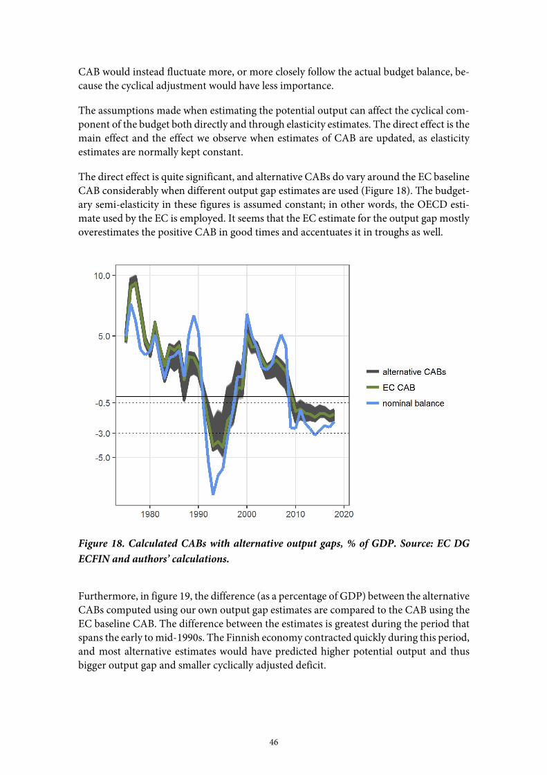
46

CAB would instead fluctuate more, or more closely follow the actual budget balance, be-cause the cyclical adjustment would have less importance.

The assumptions made when estimating the potential output can affect the cyclical com-ponent of the budget both directly and through elasticity estimates. The direct effect is the main effect and the effect we observe when estimates of CAB are updated, as elasticity estimates are normally kept constant.

The direct effect is quite significant, and alternative CABs do vary around the EC baseline CAB considerably when different output gap estimates are used (Figure 18). The budget-ary semi-elasticity in these figures is assumed constant; in other words, the OECD esti-mate used by the EC is employed. It seems that the EC estimate for the output gap mostly overestimates the positive CAB in good times and accentuates it in troughs as well.

Figure 18. Calculated CABs with alternative output gaps, % of GDP. Source: EC DG

ECFIN and authors’ calculations.

Furthermore, in figure 19, the difference (as a percentage of GDP) between the alternative CABs computed using our own output gap estimates are compared to the CAB using the EC baseline CAB. The difference between the estimates is greatest during the period that spans the early to mid-1990s. The Finnish economy contracted quickly during this period, and most alternative estimates would have predicted higher potential output and thus bigger output gap and smaller cyclically adjusted deficit.

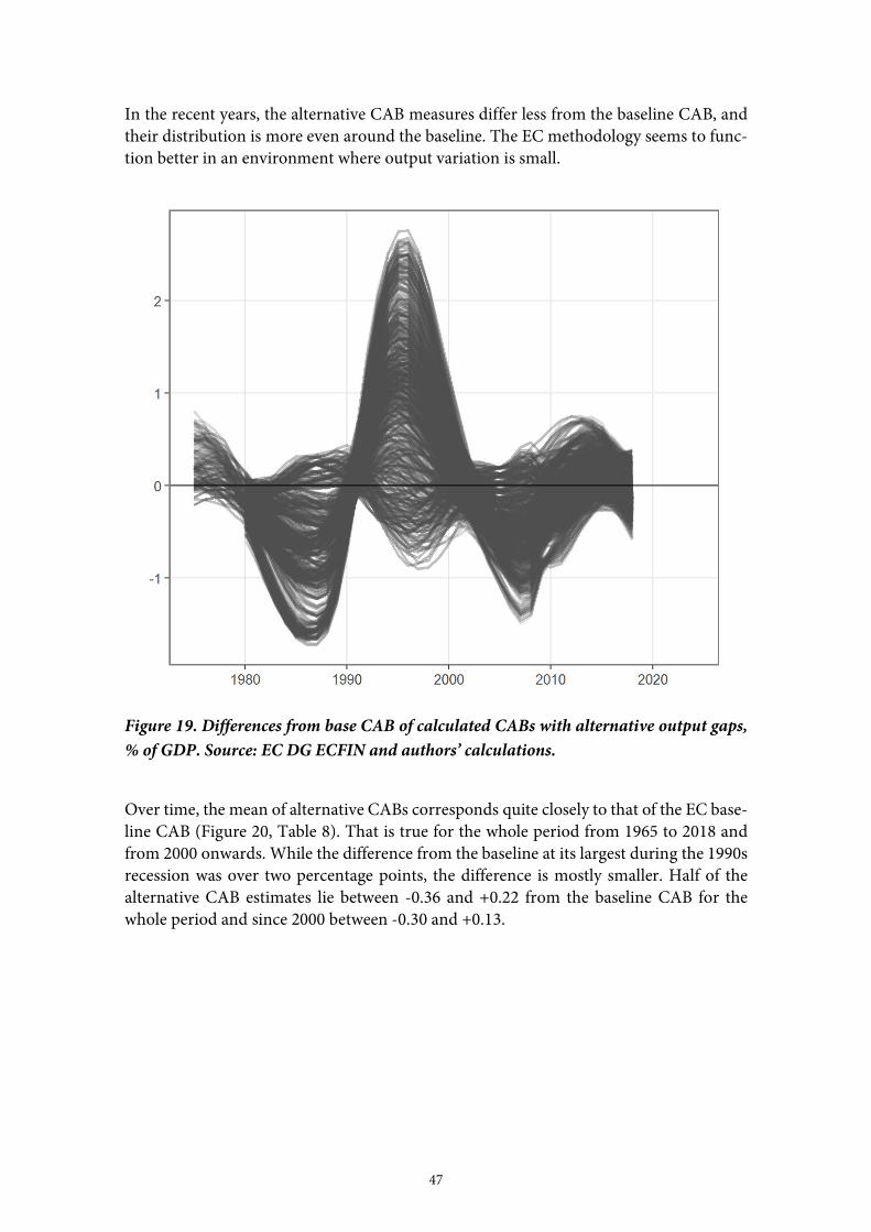
47

In the recent years, the alternative CAB measures differ less from the baseline CAB, and their distribution is more even around the baseline. The EC methodology seems to func-tion better in an environment where output variation is small.

Figure 19. Differences from base CAB of calculated CABs with alternative output gaps,

% of GDP. Source: EC DG ECFIN and authors’ calculations.

Over time, the mean of alternative CABs corresponds quite closely to that of the EC base-line CAB (Figure 20, Table 8). That is true for the whole period from 1965 to 2018 and from 2000 onwards. While the difference from the baseline at its largest during the 1990s recession was over two percentage points, the difference is mostly smaller. Half of the alternative CAB estimates lie between -0.36 and +0.22 from the baseline CAB for the whole period and since 2000 between -0.30 and +0.13.

48

Figure 20. Kernel density of differences from base CAB of calculated CABs with alterna-

tive output gaps. Source: EC DG ECFIN and authors’ calculations.

Table 8. Summary of differences of alternative CABs from base CAB.

min 25 % mean 75 % max

1965–2018 -1.72 -0.36 -0.06 0.22 2.76

2000–2018 -1.48 -0.30 -0.06 0.13 1.21

The indirect effect of output gap on CAB through elasticity estimates is relatively small. Alternative semi-elasticity estimates (ε) fall between 0.49 and 0.51. Anyhow, when using the own estimates of the semi-elasticity, the smaller individual elasticity for wages and salaries implies that the cyclical component will appear smaller in comparison to the EC estimate. Still, the effect of different elasticity estimates on the CAB are not comparable to the changes caused by the different output gaps.

If the CABs are calculated using own estimates of elasticities and the EC output gap esti-mate and are compared to the CAB calculated using the same EC output gap estimate and the semi-elasticity based on the Commission output gap (computed by the authors using

49

the revised data, 0.5116), it can be observed that the differences in the CABs due to the elasticity estimates are relatively small. When the output gap is at its largest, the larger the elasticity difference from the baseline, and the larger the effect on the CAB. In other words, the different elasticity estimates will accentuate the deviations in the CAB caused by different output gap estimates, but the effect on the CAB is relatively small.

6 Conclusions and recommendations

Estimates of the output gap and the cyclically-adjusted budget balance can vary consider-ably, depending on assumptions made in the trend estimation of the unemployment rate, participation rate, average hours worked and TFP. The most critical components are trend unemployment and participation rates.

Even if the trend unemployment rate and the TFP are estimated using the multivariate Kalman filter, it is the univariate time series estimation issues that affect the estimation the most. This is because the unit labour costs through Phillips-curve in the unemploy-ment trend estimation and the capacity utility indicator in the TFP trend estimation have a relatively small impact.

For unemployment rate, the estimation bounds to cycle and trend variances have the big-gest impact on the output gap and the CAB. Minor changes in the bounds to variance have a large effect on the trend unemployment. The bounds are even more problematic as they are hardly theoretically justified, and changes to the bounds seem to stem mainly from a desire to limit the variance from the previous EC forecast rounds.

Also, the participation rate has a relatively influential role when determining the output gap. With current estimation assumptions, the trend of participation rate very closely fol-lows the actual participation rate and in our view does not reflect the potential participa-tion rate. The actual potential participation rate is probably much flatter than the esti-mated one.

It would probably be appropriate to consider adding demographic aspects to the partici-pation rate estimation. Also, the NAWRU estimation could benefit from that. In the USA, the potential unemployment rate does take into account different behaviours of different groups in the labour market (Arnold, 2009; CBO, 2001).

However, the tested alternatives were mostly in accordance with the EC output gap esti-mation in a period with a rather stable unemployment rate. The differences grow when there are substantial changes in the unemployment rate. Mostly due to the flatter trend unemployment rate, alternative output gap series were also flatter than the EC baseline output gap.

16 The difference to the reported estimate (0.57) is mainly due to a different individual elasticity of wages and salaries.

50

The changes to the CAB caused by the changes in the budgetary semi-elasticities, induced by different output gaps, are small. However, the elasticity estimates themselves are sen-sitive to the changes in the output gap and, to a lesser extent, in the trend unemployment rate. Data revisions also play an important role in the estimation of the elasticities.

As the EC has moved toward making the trend estimation based more on economic the-ory by applying multivariate method for unemployment rate and TFP trend estimation, the estimation method has become more complicated and harder to replicate. Unfortu-nately, added complexity in estimation does not seem to add much value. Criticisms against univariate methods also apply largely to the EC method, as the Phillips curve re-lation for unemployment and the capacity relation for TFP are weak and univariate com-ponents largely determine their trend.

Output gap and cyclically adjusted budget balance are useful concepts when assessing the financial policy stance of the EU counties. Uncertainty from technical assumptions is sig-nificant, but the overall message from our alternative CAB estimates is in line with the EC estimate. In this regard, the uncertainty in real time estimation that we did not assess is more troubling (see, for example, Kuusi 2017).

However, the uncertainty and reliance on many debateable assumptions makes the role of the methodology in the EU financial policy surveillance problematic. Thus, it would be better to ascribe it a consultative role rather than a role as a binding rule.

Additionally, sparse documentation and complexity of process makes the EC method hard to replicate, and transparency is less that satisfactory. The problems are most severe in the estimation of the elasticities,17 but output gap estimation would also truly benefit from a replicable, open source process.

Moreover, in the estimation of the elasticities, the specification selection might not fully reflect the suitability of the model, since at most two of the three specifications estimations seem to fit considerably well in the data. Both error-correction specifications seem to per-form better than the AR(1), hinting at a correctly identified need to use an error-correc-tion model.

Additionally, the elasticities might require more frequent revision, since both data revi-sions and revised output gap estimates influence the estimates to some extent. The as-sumptions about the constant revenue and expenditure share to GDP as well as about the different revenue and expenditure categories’ constant shares of total revenue and ex-penditure should be reconsidered.

17 Information available on the data sources used has turned out to be insufficient. Some details of the issues encoun-

tered are listed in Table A.5 of the appendix. The model replicability could be achieved, for example, by improving documentation of the process.

51

7 References

Arnold, R. (2008), Reestimating the Phillips Curve and the NAIRU, Congressional Budget

Office Working Paper Series 2008–06.

Arnold, R. W. (2009), The challenges of estimating potential output in real time, Review

91.

Backus, D. K. and Kehoe, P. J. (1992), International evidence on the historical properties

of business cycles, The American Economic Review: 864–888.

Billmeier, A. (2006), Measuring a roller coaster: evidence on the Finnish output gap, Finn-

ish Economic Papers 19(2): 69–83.

Blanchard, O. J. (2016), The Phillips Curve: Back to the ’60s?, American Economic Review

106(5): 31–34.

Blanchard, O. J., Cerutti, E. and Summers, L. H. (2015), Inflation and activity – Two ex-

plorations and their monetary policy implications, IMF Working Paper 15/230.

Borio, C., Disyatat, F. P. and Juselius, M. (2013), Rethinking potential output: Embedding

information about the financial cycle, Bank for International Settlements Work-

ing Papers 404.

Bouis, R., Cournède, B. and Christensen, A. (2012), Implications of Output Gap Uncer-

tainty in Times of Crisis, OECD Economics Department Working Papers 977.

CBO (2001), CBO’s Method for Estimating Potential Output: An Update, Congressional

Budget Office, A CBO Paper.

Cogley, T. and Nason, J. M. (1995), Effects of the Hodrick-Prescott filter on trend and

difference stationary time series: implications for business cycle research, Journal

of Economic Dynamics and Control 19(1–2): 253–278.

Cooley, T. F. and Ohanian, L. E. (1991), The cyclical behavior of prices, Journal of Mon-

etary Economics 28(1): 25–60.

Darvas, Z. and Simon, A. (2015), Filling the gap: Open economy considerations for more

reliable potential output estimates, Bruegel Working Paper 2015/11.

Dixon, R., Lim, G. C. and Ours, J. van (2016), Revisiting Okun’s Relationship, CEPR Dis-

cussion Paper 11184.

European Commission (2016), European economic forecast: Autumn 2016, European

Economy Insitutional Paper 038.

Fabiani, S. and Mestre, R. (2000), Alternative measures of the NAIRU in the euro area:

estimates and assessment.

Farmer, R. E. (2013), The Natural Rate Hypothesis: an idea past its sell-by date, Bank of

England. Quarterly Bulletin 53(3): 244.

Fioramanti, M. (2016), Potential Output, Output Gap and Fiscal Stance: is the EC estima-

tion of the NAWRU too sensitive to be reliable?

Fioramanti, M., Padrini, F. and Pollastri, C. (2005), La stima del PIL potenziale e dell’out-

put gap: analisi di alcune criticità, Ufficio parlamentare di bilancio Nota di lavoro

1/2015.

Galí, J. (2011), The return of the wage Phillips curve, Journal of the European Economic

Association 9(3): 436–461.

52

Gechert, S., Rietzler, K. and Tober, S. (2014), The European Commission’s New NAIRU:

Does it Deliver?, Institut für Makroökonomie und Konjunkturforschung - Mac-

roeconomic Policy Institute Working Paper 142.

Girouard, N. and André, C. (2006), Measuring cyclically-adjusted budget balances for

OECD countries, available at SSRN 2005002.

Gordon, R. J. (2013), The Phillips curve is alive and well: Inflation and the NAIRU during

the slow recovery, National Bureau of Economic Research.

Hamilton, J. D. (2016), Why You Should Never Use the Hodrick-Prescott Filter, Working

Paper.

Harvey, A. and Trimbur, T. (2008), Trend estimation and the Hodrick-Prescott filter,

Journal of the Japan Statistical Society 38(1): 41–49.

Havik, K., Mc Morrow, K., Orlandi, F., Planas, C., Raciborski, R., Roeger, W., … Vander-

meulen, V. (2014), The Production Function Methodology for Calculating Poten-

tial Growth Rates & Output Gaps, European Commission Economic Papers 535.

Hodrick, R. J. and Prescott, E. C. (1997), Postwar US business cycles: an empirical inves-

tigation, Journal of Money, Credit, and Banking: 1–16.

Hristov, A. and Roeger, W. (2017), On Econometrics with a Human Face and Business

Cycles: A Reply to Fioramanti and Waldmann’s Criticism on the EU’s NAWRU

Methodology, European Economy Economic Brief 22.

Jaakkola, J. (2016), Julkisyhteisöjen rahoitustasapainon suhdanneriippuvaisten tekijöiden

ja finanssipolitiikan päätösperäisyyden arviointia, Kansantaloudellinen Aikakaus-

kirja 112(3): 297–313.

Jong, R. M. de and Sakarya, N. (2016), The Econometrics of the Hodrick-Prescott Filter,

Review of Economics and Statistics 98(2): 310–317.

Kuusi, T. (2015), Rakenteellisen rahoitusaseman mittaamisen vaihtoehtoja, Valtioneu-

voston selvitys- ja tutkimustoiminnan julkaisusarja 5/2015.

Kuusi, T. (2017), Does the Structural Budget Balance Guide Fiscal Policy Pro-Cyclically?

Evidence from the Finnish Great Depression of the 1990s, National Institute Eco-

nomic Review 239(1): R14–R31.

Logeay, C. and Tober, S. (2006), Hysteresis and the NAIRU in the Euro Area, Scottish

Journal of Political Economy 53(4): 409–429.

Marcellino, M. G. and Musso, A. (2010), Real time estimates of the euro area output gap:

Reliability and forecasting performance, European Cental Bank Working Paper

Series NO 1157.

Mc Morrow, K., Roeger, W., Vandermeulen, V. and Havik, K. (2015), An assessment of

the relative quality of the Output Gap estimates produced by the EU’s Production

Function Methodology, European Commission, Directorate-General for Eco-

nomic and Financial Affairs European Economy Discussion Paper 020.

Mourre, G., Astarita, C. and Princen, S. (2014), Adjusting the budget balance for the busi-

ness cycle: the EU methodology, Directorate General Economic and Financial Af-

fairs (DG ECFIN), European Commission European Economy – Economic Pa-

pers 536.

53

Mourre, G., Isbasoiu, G.-M., Paternoster, D. and Salto, M. (2013), The cyclically-adjusted

budget balance used in the EU fiscal framework: an update, European Commis-

sion, Directorate-General for Economic and Financial Affairs European Economy

– Economic Papers 478, Brussels.

Murray, J. (2014), Output gap measurement: judgement and uncertainty, Office for

Budget Responsibility Working paper No. 5.

Orlandi, F. (2012), Structural unemployment and its determinants in the EU countries,

European Economy Economic Papers 455.

Planas, C., Roeger, W. and Rossi, A. (2010), Does capacity utilisation help estimating the

TFP cycle?, DG ECFIN, European Commission Economic Papers 410.

Planas, C. and Rossi, A. (2015), Program GAP - Technical Description and User-manual

– Version 4.4, European Commission, Joint Research Centre Scientific and Tech-

nical Reports.

Price, R. W., Dang, T.-T., Botev, J. and others (2015), Adjusting fiscal balances for the

business cycle: New tax and expenditure elasticity estimates for OECD countries,

OECD Publishing.

Price, R. W., Dang, T.-T. and Guillemette, Y. (2014), New Tax and Expenditure Elasticity

Estimates for EU Budget Surveillance, OECD Economics Department Working

Papers 1174.

Ravn, M. O. and Uhlig, H. (2002), On adjusting the Hodrick-Prescott filter for the fre-

quency of observations, Review of Economics and Statistics 84(2): 371–376.

Rusticelli, E. (2014), Rescuing the Phillips curve: Making use of long-term unemployment

in the measurement of the NAIRU, OECD Journal: Economics Studies 2014.

54

Table A.1. List of variables and data sources used in the estimation of the expenditure

or revenue base to output gap elasticities.

Variable name Variable description Data source Link

Self-employment income Self-employment income re-

ceived by households, YSE

OECD Economic Outlook

100/AMECO

https://stats.oecd.org/In-

dex.aspx?DataSet-

Code=EO100_INTERNET#

Wages and salaries Compensation of employees,

economy total, WSSS

OECD Economic Outlook

100/AMECO

https://stats.oecd.org/In-

dex.aspx?DataSet-

Code=EO100_INTERNET#

Capital income Property income received by

households, NFD4R

OECD National Accounts

Statistics (SNA93), data for

1990-2012

http://stats.oecd.org/#

Gross operating surplus GDP-TIND+TSUB-WSSS

Taxes on production and im-

ports, value (TIND)

Subsidies, value (TSUB)

Compensation of employees

(WSSS)

GDP:

OECD Economic Outlook

100/AMECO

TIND:

OECD Economic Outlook

100/AMECO

TSUB:

AMECO(/OECD National

Accounts)

https://stats.oecd.org/In-

dex.aspx?DataSet-

Code=EO100_INTERNET#,

http://stats.oecd.org/#,

http://ec.europa.eu/econ-

omy_finance/db_indica-

tors/ameco/archive_en.htm

Unemployment Unemployment rate, UNR OECD Economic Outlook

100

https://stats.oecd.org/In-

dex.aspx?DataSet-

Code=EO100_INTERNET#

Output Gross domestic product,

value, market prices, GDP

OECD Economic Outlook

100/AMECO

https://stats.oecd.org/In-

dex.aspx?DataSet-

Code=EO100_INTERNET#

Potential output Potential output at constant

prices

AMECO http://ec.europa.eu/econ-

omy_finance/db_indica-

tors/ameco/archive_en.htm

NAIRU/NAWRU Equilibrium Unemployment

rate, NAIRU (OECD)

OECD Economic Outlook

100/AMECO

https://stats.oecd.org/In-

dex.aspx?DataSet-

Code=EO100_INTERNET#

The data comprises a period of 1990–2013 unless otherwise stated and is available from OECD Economic Outlook 100,

AMECO (Autumn 2016) and OECD National Accounts Statistics (SNA93). The data sources are the same as quoted in

the Commission calculations (see Mourre et al. 2014), but the latest revision is used for all variables if available.

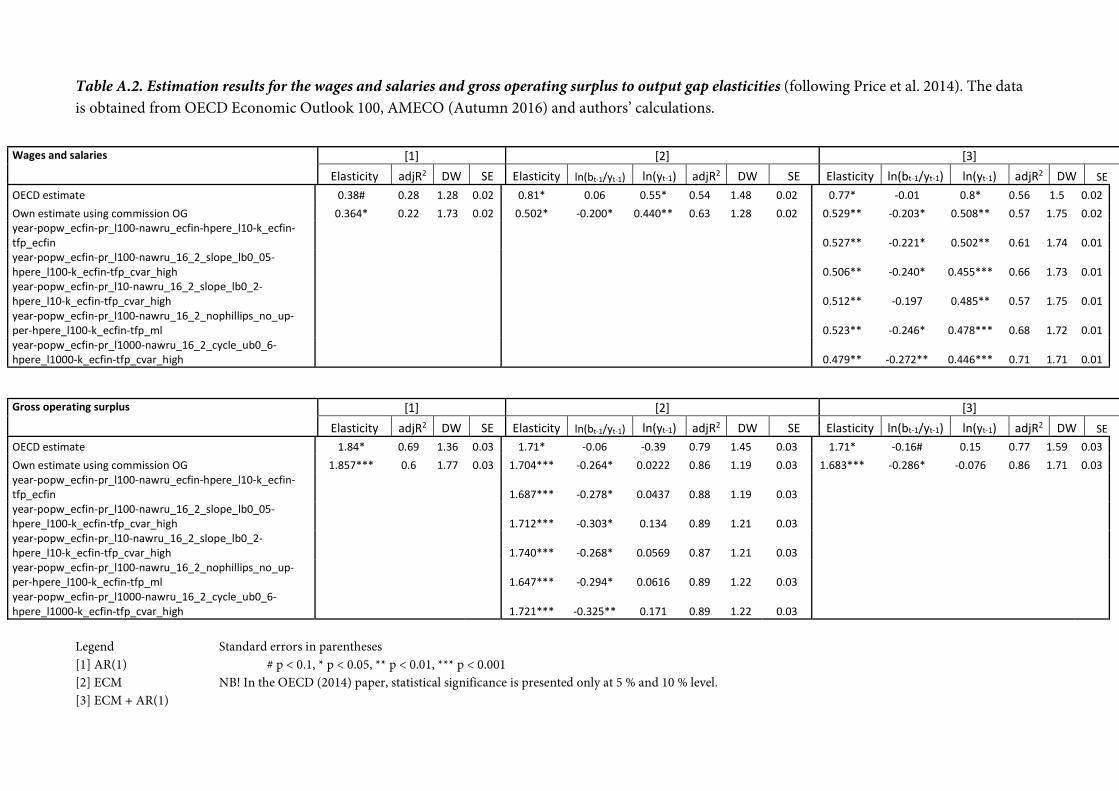
Table A.2. Estimation results for the wages and salaries and gross operating surplus to output gap elasticities (following Price et al. 2014). The data

is obtained from OECD Economic Outlook 100, AMECO (Autumn 2016) and authors’ calculations.

Legend Standard errors in parentheses

[1] AR(1) # p < 0.1, * p < 0.05, ** p < 0.01, *** p < 0.001

[2] ECM NB! In the OECD (2014) paper, statistical significance is presented only at 5 % and 10 % level.

[3] ECM + AR(1)

Wages and salaries [1] [2] [3]

Elasticity adjR2 DW SE Elasticity ln(bt-1/yt-1) ln(yt-1) adjR2 DW SE Elasticity ln(bt-1/yt-1) ln(yt-1) adjR2 DW SE OECD estimate 0.38# 0.28 1.28 0.02 0.81* 0.06 0.55* 0.54 1.48 0.02 0.77* -0.01 0.8* 0.56 1.5 0.02

Own estimate using commission OG 0.364* 0.22 1.73 0.02 0.502* -0.200* 0.440** 0.63 1.28 0.02 0.529** -0.203* 0.508** 0.57 1.75 0.02 year-popw_ecfin-pr_l100-nawru_ecfin-hpere_l10-k_ecfin-tfp_ecfin 0.527** -0.221* 0.502** 0.61 1.74 0.01 year-popw_ecfin-pr_l100-nawru_16_2_slope_lb0_05-hpere_l100-k_ecfin-tfp_cvar_high 0.506** -0.240* 0.455*** 0.66 1.73 0.01 year-popw_ecfin-pr_l10-nawru_16_2_slope_lb0_2-hpere_l10-k_ecfin-tfp_cvar_high 0.512** -0.197 0.485** 0.57 1.75 0.01 year-popw_ecfin-pr_l100-nawru_16_2_nophillips_no_up-per-hpere_l100-k_ecfin-tfp_ml 0.523** -0.246* 0.478*** 0.68 1.72 0.01 year-popw_ecfin-pr_l1000-nawru_16_2_cycle_ub0_6-hpere_l1000-k_ecfin-tfp_cvar_high 0.479** -0.272** 0.446*** 0.71 1.71 0.01

Gross operating surplus [1] [2] [3]

Elasticity adjR2 DW SE Elasticity ln(bt-1/yt-1) ln(yt-1) adjR2 DW SE Elasticity ln(bt-1/yt-1) ln(yt-1) adjR2 DW SE OECD estimate 1.84* 0.69 1.36 0.03 1.71* -0.06 -0.39 0.79 1.45 0.03 1.71* -0.16# 0.15 0.77 1.59 0.03

Own estimate using commission OG 1.857*** 0.6 1.77 0.03 1.704*** -0.264* 0.0222 0.86 1.19 0.03 1.683*** -0.286* -0.076 0.86 1.71 0.03 year-popw_ecfin-pr_l100-nawru_ecfin-hpere_l10-k_ecfin-tfp_ecfin 1.687*** -0.278* 0.0437 0.88 1.19 0.03 year-popw_ecfin-pr_l100-nawru_16_2_slope_lb0_05-hpere_l100-k_ecfin-tfp_cvar_high 1.712*** -0.303* 0.134 0.89 1.21 0.03 year-popw_ecfin-pr_l10-nawru_16_2_slope_lb0_2-hpere_l10-k_ecfin-tfp_cvar_high 1.740*** -0.268* 0.0569 0.87 1.21 0.03 year-popw_ecfin-pr_l100-nawru_16_2_nophillips_no_up-per-hpere_l100-k_ecfin-tfp_ml 1.647*** -0.294* 0.0616 0.89 1.22 0.03 year-popw_ecfin-pr_l1000-nawru_16_2_cycle_ub0_6-hpere_l1000-k_ecfin-tfp_cvar_high 1.721*** -0.325** 0.171 0.89 1.22 0.03

56

Table A.3. Estimation results for the capital income and unemployment to output gap elasticities (following Price et al. 2014). The data is obtained

from OECD Economic Outlook 100, AMECO (Autumn 2016), authors’ calculations and for capital income from OECD Annual National Accounts,

SNA93.

Legend Standard errors in parentheses

[1] AR(1) # p < 0.1, * p < 0.05, ** p < 0.01, *** p < 0.001

[2] ECM NB! In the OECD (2014) paper, statistical significance is presented only at 5 % and 10 % level.

[3] ECM + AR(1)

Capital income [1] [2] [3] Elasticity adjR2 DW SE Elasticity ln(bt-1/yt-1) ln(yt-1) adjR2 DW SE Elasticity ln(bt-1/yt-1) ln(yt-1) adjR2 DW SE

OECD estimate 3.06# 0.26 1.96 0.12 3.34* -0.13 2.96* 0.51 1.97 0.1 3.75* -0.13 2.84* 0.51 2.01 0.1 Own estimate using commission OG 2.276* 0.24 1.737 0.12 4.099** 0.107 2.993** 0.48 2.03 0.09 4.080** 0.112 2.999** 0.49 2.00 0.09 year-popw_ecfin-pr_l100-nawru_ecfin-hpere_l10-k_ecfin-tfp_ecfin 4.064** 0.12 2.738** 0.47 2.05 0.09 year-popw_ecfin-pr_l100-nawru_16_2_slope_lb0_05-hpere_l100-k_ecfin-tfp_cvar_high 3.541** 0.102 2.104** 0.46 1.93 0.10 year-popw_ecfin-pr_l10-nawru_16_2_slope_lb0_2-hpere_l10-k_ecfin-tfp_cvar_high 3.903** 0.1 2.785** 0.46 1.97 0.10 year-popw_ecfin-pr_l100-nawru_16_2_nophillips_no_upper-hpere_l100-k_ecfin-tfp_ml 3.647** 0.124 2.103** 0.45 1.92 0.10 year-popw_ecfin-pr_l1000-nawru_16_2_cycle_ub0_6-hpere_l1000-k_ecfin-tfp_cvar_high 3.229* 0.0811 1.677** 0.42 1.82 0.10 Unemployment [1] [2] [3]

Elasticity adjR2 DW SE Elasticity ln(bt-1/yt-1) ln(yt-1) adjR2 DW SE Elasticity ln(bt-1/yt-1) ln(yt-1) adjR2 DW SE OECD estimate -2.3* 0.73 2.09 0.06 -3.66* -0.63* -4.09* 0.86 0.7 0.05 -3.01* -0.56* -3.48* 0.9 2.44 0.04 Own estimate using commission OG -2.822*** 0.6 1.672 0.07 -3.517*** -0.571*** -3.476*** 0.86 0.96 0.05 -2.835*** -0.686*** -3.391*** 0.88 2.08 0.04 year-popw_ecfin-pr_l100-nawru_ecfin-hpere_l10-k_ecfin-tfp_ecfin -2.973*** -0.720*** -3.697*** 0.88 2.01 0.04 year-popw_ecfin-pr_l100-nawru_16_2_slope_lb0_05-hpere_l100-k_ecfin-tfp_cvar_high -3.228*** -0.675*** -3.842*** 0.89 2.24 0.04 year-popw_ecfin-pr_l10-nawru_16_2_slope_lb0_2-hpere_l10-k_ecfin-tfp_cvar_high -2.805*** -0.675*** -3.466*** 0.87 2.10 0.04 year-popw_ecfin-pr_l100-nawru_16_2_nophillips_no_upper-hpere_l100-k_ecfin-tfp_ml -3.481*** -0.642*** -4.072*** 0.89 2.31 0.04 year-popw_ecfin-pr_l1000-nawru_16_2_cycle_ub0_6-hpere_l1000-k_ecfin-tfp_cvar_high -3.090*** -0.668*** -3.746*** 0.89 2.05 0.04

57

Table A.4. The budgetary semi-elasticities calculated using the Commission output gap estimates and various own estimates of the output gap (1-

5).

1) year-popw_ecfin-pr_l100-nawru_ecfin-hpere_l10-k_ecfin-tfp_ecfin

2) year-popw_ecfin-pr_l100-nawru_16_2_slope_lb0_05-hpere_l100-k_ecfin-tfp_cvar_high

3) year-popw_ecfin-pr_l10-nawru_16_2_slope_lb0_2-hpere_l10-k_ecfin-tfp_cvar_high

4) year-popw_ecfin-pr_l100-nawru_16_2_nophillips_no_upper-hpere_l100-k_ecfin-tfp_ml

5) year-popw_ecfin-pr_l1000-nawru_16_2_cycle_ub0_6-hpere_l1000-k_ecfin-tfp_cvar_high

Elasticity of: Weights (% of GDP) Semi elasticity for:

Revenue level Expenditure level Revenue-to-GDP

ratio Expenditure-to-GDP ra-

tio: Total revenue Total expen-

diture Revenue Expenditure Budget balance

Benchmark 0.942 -0.182 -0.058 -1.182 53.13 % 51.08 % -0.031 -0.604 0.57304 EC OG 0.855 -0.141 -0.145 -1.141 53.13 % 51.08 % -0.077 -0.583 0.50599 1 0.854 -0.148 -0.146 -1.148 53.13 % 51.08 % -0.078 -0.586 0.50869 2 0.833 -0.161 -0.167 -1.161 53.13 % 51.08 % -0.089 -0.593 0.50395 3 0.843 -0.140 -0.157 -1.140 53.13 % 51.08 % -0.083 -0.582 0.49881 4 0.843 -0.173 -0.157 -1.173 53.13 % 51.08 % -0.083 -0.599 0.51585 5 0.814 -0.154 -0.186 -1.154 53.13 % 51.08 % -0.099 -0.589 0.49045

Table A.5. Technical problems encountered with the data and the estimation relating

to the elasticities.

Problem Implication Solution

The OECD will not supply

the original data used in the

estimation.

The replication of compu-

tations of the elasticities is

difficult.

Use publicly available data

and the most recent revi-

sions from OECD Eco-

nomic Outlook, AMECO.

In the publicly available

data sources, the most re-

cent revisions do not fully

correspond to the series re-

ported by the OECD.

No clear indication for the

type of data to be used; rep-

lication and application

troubled.

Tests using diverse types of

data, e.g. when it comes to

sectors (household vs.

whole economy).

Accurate description of es-

timation models is not

available from the OECD.

Resort to general under-

standing of the models

based on the vague descrip-

tions in the working pa-

pers.

Various alternative models

tested and different as-

sumptions within the mod-

els considered.