TRUE COLOR BVR IMAGING by Heidi Dumais … · Heidi Dumais This thesis has been reviewed by the research committee, senior thesis coordinator, and department chair and has been found

TRUE COLOR BVR IMAGING

FROM ASTRONOMICAL EXPOSURES

by

Heidi Dumais

A senior thesis submitted to the faculty of

Brigham Young University – Idaho

in partial fulfillment of the requirements for the degree of

Bachelor of Science

Department of Physics

Brigham Young University - Idaho

December 2008

Copyright © 2008 Heidi Dumais

All Rights Reserved

BRIGHAM YOUNG UNIVERSITY – IDAHO

DEPARTMENT APPROVAL

of a senior thesis submitted by

Heidi Dumais

This thesis has been reviewed by the research committee, senior thesis coordinator, and department chair and has been found to be satisfactory.

Date Stephen McNeil, Advisor Date David Oliphant, Senior Thesis Coordinator Date Brian Tonks, Committee Member Date Stephen Turcotte, Chair

ABSTRACT

TRUE COLOR BVR IMAGING FROM ASTRONOMICAL EXPOSURES

Heidi Dumais

Department of Physics

Bachelor of Science This paper explores various astronomical BVR image color balance techniques in an attempt to find an acceptable version of “true color.” The definition of true color images remains an elusive concept. Color depends on filter transmission, detector quantum efficiency, and the geometry of the telescope in addition to the variable response of the human eye to color and light levels. Abandoning any hope of addressing the last issue in the time allotted, the total system efficiency can be determined based upon the first three functions. This provides a dimensionless value which can be used to the find relative color balance coefficients. However, a simpler method involves modeling the filter passbands as Gaussian curves and finding the average value of the quantum efficiency for each color filter. The resulting color coefficients, including error estimations, work as well as the total system efficiency, but with greater ease.

ACKNOWLEDGMENTS

Partial funding for this research was provided by the National Science Foundation through the Research Experience for Undergraduates program at Brigham Young University, grant PHY-0552795.

Partial funding was also provided by Dr. J. Ward Moody of the Brigham Young University Physics and Astronomy Department.

Some of the data presented in this paper was obtained from the Multimission Archive at the Space Telescope Science Institute (MAST). STScI is operated by the Association of Universities for Research in Astronomy, Inc., under NASA contract NAS5-26555. Support for MAST for non-HST data is provided by the NASA Office of Space Science via grant NAG5-7584 and by other grants and contracts.

xi

Contents

Contents ...................................................................................................................................... xi

List of Figures ..............................................................................................................................xiii

1 Introduction ............................................................................................................................... 1

2 Color Imaging ............................................................................................................................. 3

2.1 Digital Color Photography .................................................................................................. 3

2.2 Filter Passbands .................................................................................................................. 4

2.3 Quantum Efficiency ............................................................................................................ 6

2.4 Telescope Geometry ........................................................................................................... 7

2.5 Atmospheric Scattering ...................................................................................................... 8

3 Color Balance Methods ........................................................................................................... 11

3.1 Commercial Software ....................................................................................................... 12

3.2 Total System Throughput ................................................................................................. 15

3.3 Gaussian Model ................................................................................................................ 16

3.4 Approximate System Throughput .................................................................................... 18

4 Ground Based Example............................................................................................................ 21

5 Conclusions .............................................................................................................................. 23

Bibliography ................................................................................................................................ 25

Appendix A: Coefficient Calculation for Gaussian Model ........................................................... 27

Appendix B: Summation Method Coefficient Calculation .......................................................... 31

xiii

List of Figures

Figure 1. 1: Orion Nebula calculated color balance..................................................................................... 2

Figure 2. 1: Passband plots for standard Johnson photometric filters. ......................................................... 5

Figure 2. 2: Quantum efficiency plot for an SBIG ST-10XME detector. .................................................... 7

Figure 2. 3: System throughput plot for the WFPC2 detectors. ................................................................... 8

Figure 2. 4: Difference in quantum efficiency between the WF and PC detectors. ..................................... 8

Figure 3. 1: Cosmic rays removed before color balance. ........................................................................... 14

Figure 3. 2: Cosmic rays removed after color balance. ............................................................................. 14

Figure 3. 3: Passband plots for WFPC2 F814W, F606W, and F450W respectively. ................................ 17

Figure 4. 1: AstroArt auto-balance. ........................................................................................................... 22

Figure 4. 2: Calculated color balance. ....................................................................................................... 22

1

Chapter 1

Introduction

Viewers of astronomical images often wonder if the majestic nebulae really appear

so detailed and colorful. Looking through a telescope at the same objects leaves

doubt that they were displayed accurately in the color images. In terrestrial digital

photography, the images can be qualitatively compared to the actual scenes to

determine how well the camera’s chip represents nature. However, a trip to

another galaxy to determine the validity of someone’s photographic rendition of

said galaxy would seem unlikely. And so the question arises, how do astronomers

know what color to assign the galaxy? And what does the phrase “true color”

actually mean?

Another question might be why it matters if the colors are “real.” A well

balanced tri-color image can reveal a lot about the composition and temperature

of an astronomical object in one simple image. For example, an intense region of

red in an image could indicate a large amount of electron transitions from the n=3

to n=2 states in formerly ionized Hydrogen. As another example, Figure 1.1 shows

green regions in the Orion Nebula surrounding a group of four stars called the

Trapezium. These stars heat the region around them causing a greener color than

the surrounding red areas (which have a lower temperature). The color balance

technique used to produce this image will be discussed in detail in section 3.3.

2 Chapter 1 Introduction

Interestingly, a lot images of this object which are not color balanced according to

any precise definition of true color appear much redder and miss the green

regions surrounding the Trapezium.

Figure 1. 1: Orion Nebula calculated color balance.

This research explores various astronomical image color balance

techniques in an attempt to determine a few definitions of “true color” as it applies

to astronomy and how the validity these color balance methods compare. These

methods include using commercial software, a total system throughput, an

approximated system throughput, and modeling filter passbands as Gaussian

curves with an average value for the quantum efficiency.

3

Chapter 2

Color Imaging

2.1 Digital Color Photography

A large gap exists between how the human eye views the universe and how

Charge Coupled Devices (CCD cameras) record it. For the eye, color sensitivity

depends on the overall light levels. During twilight, “photochemical changes in the

eyes, pupil dilation from 2.5 to nearly 7mm, and the shift to scotopic

[monochromatic vision due to low light levels] rod-cell vision make the transition

so smooth, we'd never guess that ambient illumination during early astronomical

twilight has grown 500,000 times dimmer than when the Sun was shining.” [7] In

addition to losing color sensitivity at low light levels, at higher light levels red and

yellow become predominate. Also, staring at the same object for prolonged

periods does not appear to increase the brightness of the object. The human eye’s

variable refresh rate, affected by both light levels and color, changes the

perception of objects and their color. However, with CCD images the color

sensitivity remains a constant function of the wavelength, and increasing the

exposure time predictably increases the image brightness. A great deal of research

4 Chapter 2 Color Imaging

funded mostly by the digital camera industry delves into attempts to replicate the

human eye response to color in a CCD chip.

In general, a CCD chip contains a large number of silicon based

photosensors called pixels. As photons strike the pixel electrons jump up energy

levels and become trapped in a potential well. At the end of the exposure, a

computer counts the number of trapped electrons in each pixel and assigns it that

value. This process gives the image a great deal of dynamic range: both bright and

dim objects can be recorded in the same field. In color CCD chips, the same process

applies with various modifications. One method involves coating individual pixels

with a substance sensitive to a specific color. An array of pixels, each sensitive to

red, blue or green, counts the electrons for each pixel and an algorithm assigns

each group a color value based on how many counts each color pixel recorded.

Sony developed a four color CCD chip which instead of just green, included pixels

sensitive to the color “emerald” [3] in an attempt to more closely match the human

eye’s color sensitivity. Other methods include beam splitters and multiple filtered

CCD chips, or CCDs which record the color based upon penetration depth of the

photons. The attempt to develop better color for digital cameras which display

images in “true color” continues.

2.2 Filter Passbands

A description of light transmission of a filter verses the wavelength of light is

called a passband. Figure 2.1 shows the passband curves for the standard Johnson

filter set. These plots will be utilized later for color balance calculations discussed

in chapter 5.

5

Figure 2. 1: Passband plots for standard Johnson photometric filters [adapted from 8].

Different filter types carry different transmission curves associated with

their passband plots. For use in astronomical exposures, different passband types

will provide different types of images. For example, if an astronomer were

researching the distribution of particular elements, narrow band filters can be

used. Narrow band filters allow a very small range of wavelengths to reach the

detector, thereby recording only the information of interest, such as the emission

lines of a particular element. In contrast, a broadband filter allows a larger range

of wavelengths to reach the detector.

Exposures taken with broadband filters for three different peak

wavelengths provide the data for tricolor images. In general, an ideal tricolor filter

set would have uniform transmission over a specific domain of wavelengths, and

essentially no transmission everywhere else. Also, a set of tricolor filters should

not have overlap between transmission curves. This would lead to a redundancy

of information at the overlapping wavelengths. Similarly, gaps between filter

passbands leave out color information. A perfect combination of color filter

passbands would have a flat line across the visible wavelengths and drop off


sharply at the edges. Obviously the passbands shown in Figure 2.1 don’t match

that description.

The filter passbands shown in Figure 2.1 corresponding to the B, V, and R

filters do not represent a perfectly ideal set of color filters. However, they do

provide a good one. The curves do not drop off at a perfect vertical line but they

do have a steep slope. While there is still overlap between two adjacent filter

passbands, the steeper slope lowers that amount of overlap. Also, a high value for

the slope on the outer edges of the B and R filters means the curves do not extend

very far into the ultraviolet or infrared ranges. Overall, the BVR Johnson

photometric filters have relatively low redundancy, cover the entire visual range

of wavelengths, and do not include very much UV or IR information.

2.3 Quantum Efficiency

The sensitivity of a CCD detector to incident light depends on the energy (and

therefore wavelength) of that light. The fraction of light detected by the

photosensor array, called the quantum efficiency of the CCD, is often displayed as

a plot against the wavelength of incident light. Typical shapes for quantum

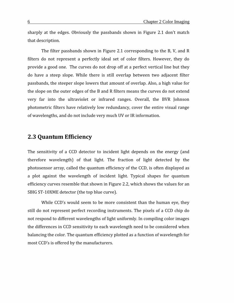
efficiency curves resemble that shown in Figure 2.2, which shows the values for an

SBIG ST-10XME detector (the top blue curve).

While CCD’s would seem to be more consistent than the human eye, they

still do not represent perfect recording instruments. The pixels of a CCD chip do

not respond to different wavelengths of light uniformly. In compiling color images

the differences in CCD sensitivity to each wavelength need to be considered when

balancing the color. The quantum efficiency plotted as a function of wavelength for

most CCD’s is offered by the manufacturers.

7

Figure 2. 2: Quantum efficiency plot for an SBIG ST-10XME detector [adapted from 9].

2.4 Telescope Geometry

Another related and perhaps more useful plot describes how a specific telescope

and CCD register incident light. This value, referred to as a system throughput,

includes the effects of telescope geometry including mirrors and lenses. Figure 2.3

shows a plot of the system throughput for the Hubble Space Telescope Wide Field

and Planetary Camera 2 (WFPC2) detectors. (As an interesting side note, this

system throughput represents the quantum efficiency for three of the four

detectors in the WFPC2 array. The quantum efficiency of the “PC corner” shown in

Figure 2.4 is not well represented by this plot, which becomes evident after

applying color to a WFPC 2 image and that section of the object appears to have

different colors than the rest of the object.)


Figure 2. 3: System throughput plot for the WFPC2 detectors [adapted from 4].

Figure 2. 4: Difference in quantum efficiency between the WF and PC detectors.

2.5 Atmospheric Scattering

For ground based data the atmosphere has a non-negligible effect on the CCD

counts at different wavelengths. Shorter wavelengths will scatter more,

specifically, the relative scattering of different wavelengths varies as

9

4

1

P (2.1)

where is the wavelength in meters [2]. Using Equation (2.1), blue light (= 450

nm) scatters 5.9 times as much as red light ( = 700 nm). However, the angle of

the detector with respect to the horizon changes the magnitude of the color

alteration. For example, directly above the horizon light must travel through 13

times more air than when it is directly overhead (the zenith). [7] At these low

altitudes the shorter wavelengths scatter, leaving more red colors. At the zenith,

the scattering of each wavelength is essentially the same. For the purposes of

astronomical images, shooting near the horizon causes so much distortion that the

FWHM values for stars render the data unreliable. Generally, keeping the shooting

angle near the zenith would make any differences in atmospheric scattering

negligible for most purposes.


11

Chapter 3

Color Balance Methods

Due to a requirement for large amounts of tri-color images from the same

telescope, detector and filters, this research utilized data from the WFPC2 array on

the Hubble Space Telescope. A survey of star forming galaxies provided a set of

images with both uniform exposure time and the three color images required for

this research. A selection of 15 galactic image sets provided the data for the color

balance techniques explored during the course of the space telescope portion of

this project. The research included exposures from the F450W, F606W and

F814W filters. The number in the filter names indicates the peak wavelength of

light transmission for the filter in nanometers. Calibration techniques do not

directly relate to this research, so pre-calibrated data was used. (For Hubble

Legacy Archive calibration procedures please consult the Space Telescope Science

Institute [10]).

For this research the software programs IRAF, AstroArt, Excel, Maple 11

and Photoshop CS3 provided the means of data processing. The WFPC 2 data was

initially converted into compatible files and registered (lined up) into a mosaic

using IRAF. Some of the data also had cosmic rays removed using IRAF. Excel and

12 Chapter 3 Color Balance Methods

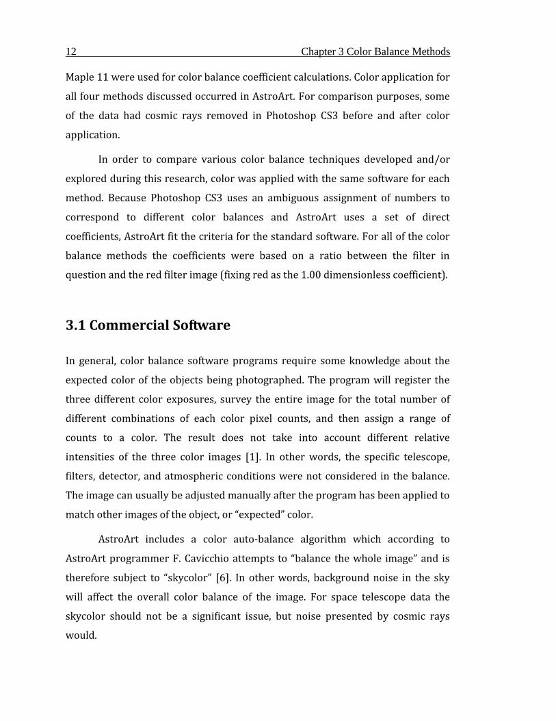
Maple 11 were used for color balance coefficient calculations. Color application for

all four methods discussed occurred in AstroArt. For comparison purposes, some

of the data had cosmic rays removed in Photoshop CS3 before and after color

application.

In order to compare various color balance techniques developed and/or

explored during this research, color was applied with the same software for each

method. Because Photoshop CS3 uses an ambiguous assignment of numbers to

correspond to different color balances and AstroArt uses a set of direct

coefficients, AstroArt fit the criteria for the standard software. For all of the color

balance methods the coefficients were based on a ratio between the filter in

question and the red filter image (fixing red as the 1.00 dimensionless coefficient).

3.1 Commercial Software

In general, color balance software programs require some knowledge about the

expected color of the objects being photographed. The program will register the

three different color exposures, survey the entire image for the total number of

different combinations of each color pixel counts, and then assign a range of

counts to a color. The result does not take into account different relative

intensities of the three color images [1]. In other words, the specific telescope,

filters, detector, and atmospheric conditions were not considered in the balance.

The image can usually be adjusted manually after the program has been applied to

match other images of the object, or “expected” color.

AstroArt includes a color auto-balance algorithm which according to

AstroArt programmer F. Cavicchio attempts to “balance the whole image” and is

therefore subject to “skycolor” [6]. In other words, background noise in the sky

will affect the overall color balance of the image. For space telescope data the

skycolor should not be a significant issue, but noise presented by cosmic rays

would.

13

Attempting to balance the entire image with no information about the

filters or detector would become a problem for images with noise. Cosmic rays

have a large impact on the color balance coefficients employed by AstroArt, as

shown in Table 3.1. With the coefficient for red set at a standard (1.00) for all of

the objects, the coefficients in the columns labeled “nf” correspond to images not

filtered for hotspots or cosmic rays before color balance, while the coefficients not

labeled “nf” represent the values obtained for filtered exposures. Ideally, the

coefficients should be entirely independent of noise (especially for the same

exposures).

Table 3.1: AstroArt color balance coefficients for filtered and unfiltered Hubble images.

OBJECT GREEN GREEN(nf) BLUE BLUE(nf)

NGC1073 0.61 0.70 2.46 2.09

NGC2283 0.76 0.84 2.66 2.47

NGC1084 0.52 0.77 2.79 2.75

NGC2442 0.80 1.00 2.86 2.43

IC396 0.69 0.82 3.44 3.22

IC239 0.69 0.56 2.41 2.32

NGC4123 0.66 0.66 3.15 1.56

NGC5300 0.67 0.75 2.47 1.37

NGC5112 0.59 0.69 1.89 1.97

NGC4790 0.60 0.87 2.13 1.69

NGC4416 0.63 0.63 2.34 1.92

UGC6983 0.63 1.18 2.24 2.34

NGC4393 0.61 0.66 1.79 0.88

UGC9215 0.59 0.63 1.92 1.49

NGC4525 0.73 0.95 2.54 2.43

Mean 0.65 0.78 2.47 2.06

0.1 0.2 0.5 0.6

The mean and standard deviation for the green and blue color coefficients

are shown for both the filtered and unfiltered datasets, and match within 16.5%

and 19.9% respectively. That type of inconsistency does not build confidence in

that particular color balance technique as being “true color,” in that the same

objects have different colors depending upon how many cosmic rays happened to


strike the CCD during the exposure. This would be equivalent to assigning the

same tree different colors based upon how many fireflies passed the camera

during the exposure. Figures 3.1 and 3.2 illustrate this ambiguity in AstroArt color

balance. The cosmic rays in each filter image for Figure 3.1 were removed before

applying the color using AstroArt. The same data was used to compile Figure 3.2 in

AstroArt, leaving the cosmic rays to be removed after color application. The values

obtained for the color coefficients between the two identical images varied by

26%.

Figure 3. 1: Cosmic rays removed before color balance.

Figure 3. 2: Cosmic rays removed after color balance.

15

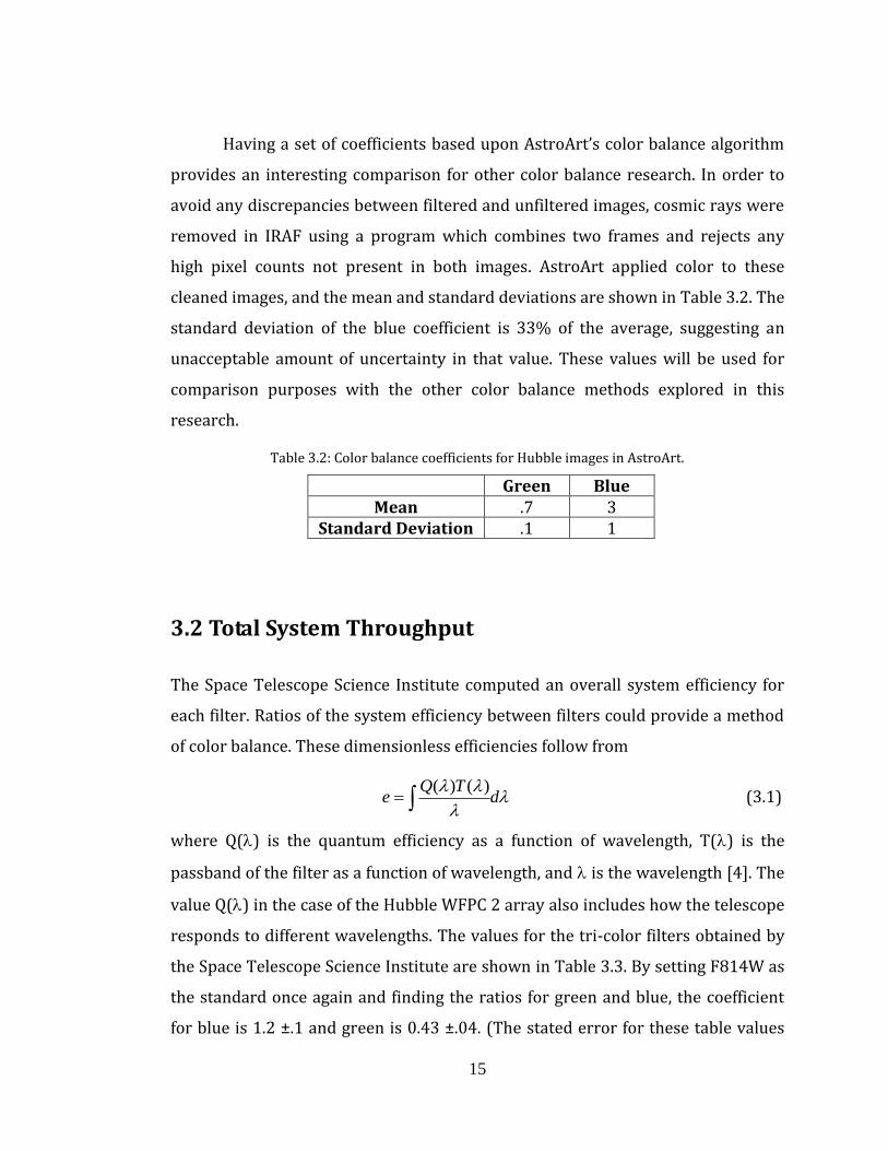
Having a set of coefficients based upon AstroArt’s color balance algorithm

provides an interesting comparison for other color balance research. In order to

avoid any discrepancies between filtered and unfiltered images, cosmic rays were

removed in IRAF using a program which combines two frames and rejects any

high pixel counts not present in both images. AstroArt applied color to these

cleaned images, and the mean and standard deviations are shown in Table 3.2. The

standard deviation of the blue coefficient is 33% of the average, suggesting an

unacceptable amount of uncertainty in that value. These values will be used for

comparison purposes with the other color balance methods explored in this

research.

Table 3.2: Color balance coefficients for Hubble images in AstroArt.

Green Blue Mean .7 3

Standard Deviation .1 1

3.2 Total System Throughput

The Space Telescope Science Institute computed an overall system efficiency for

each filter. Ratios of the system efficiency between filters could provide a method

of color balance. These dimensionless efficiencies follow from

d

TQe

)()( (3.1)

where Q() is the quantum efficiency as a function of wavelength, T() is the

passband of the filter as a function of wavelength, and is the wavelength [4]. The

value Q() in the case of the Hubble WFPC 2 array also includes how the telescope

responds to different wavelengths. The values for the tri-color filters obtained by

the Space Telescope Science Institute are shown in Table 3.3. By setting F814W as

the standard once again and finding the ratios for green and blue, the coefficient

for blue is 1.2 ±.1 and green is 0.43 ±.04. (The stated error for these table values


was 10% [4].) Section 3.3 will discuss how these values agree with those found by

modeling the passband as a Gaussian, which cuts down on time and does not

require as much detailed knowledge of the filter passbands or the detector.

Table 3.3: System Efficiencies and Zeropoints [4].

Filter QT d

/ QTmax d/d

p < > max

me/sec twfsky

F450W 0.01678 4483.6 950.8 0.0901 0.08671 36.36 4555.4 4573.0 5069 24.06 2.0E+03

F606W 0.04513 5860.1 1502.4 0.1089 0.14220 69.46 5996.8 6030.8 6185 25.13 4.2E+02

F814W 0.01949 7904.8 1539.4 0.0827 0.10343 54.06 8012.2 8040.3 7255 24.22 6.5E+02

3.3 Gaussian Model

It would seem that in order to avoid ambiguity in color balance, the coefficients

would need to be calculated based upon specific filter, telescope and detector

information (like the total system throughput). The passband graphs for the three

filters for the Hubble WFPC 2 visual tricolor data are shown in Figure 3.3. These

filters present a very good set of tri-color filters. The curves are essentially vertical

at the passband edges, with nearly constant transmission between. There is some

overlap between the filters, but no gaps.

For the purposes of color balance the useful information from the graphs in

Figure 3.3 would be the ratio of total light transmission between each filter. This

information can be obtained by modeling these passbands as Gaussian curves and

integrating the functions to obtain a quantity related to the total light transmission

of the filter. Obviously the graphs in Figure 3.3 do not resemble Gaussian curves,

however by preserving the width and peak, the ratios of their areas would be

within reasonable error. The command under the Synphot package in IRAF used

the Marquardt method to fit the passband information to a Gaussian curve [12].

Appendix A includes the complete calculation in Maple syntax which will be

outlined in this section.

17

Figure 3. 3: Passband plots for WFPC2 F814W, F606W, and F450W respectively [adapted from 5].

Having determined the Gaussian parameters in IRAF, Maple calculated the

area under the curves around the mean with a radius of five times the standard

deviation. The resulting value can be considered the total transmission of the

filter,

dxeT

x

5

5

2

)(2

2

. (3.2)

The limits of integration avoided including unrealistic contributions of the

Gaussian model at x values far from the average, , by staying within 5 standard

deviations, , of the mean. Setting red as the standard coefficient equal to one, the

red integral divided by the green and blue integrals provided their respective

transmission coefficients.

In order to find the complete color coefficients the quantum efficiency of

the detector at each wavelength had to be considered as well. The system

efficiency plot in Figure 2.3 shows how the Hubble space telescope and the WFPC2

detectors respond to different wavelengths. The quantum efficiency coefficients

were determined using the average value for the system efficiency over the width

of each filter passband, again setting red as the standard. The final color coefficient

equaled the product of the transmission and quantum efficiency coefficients. The

final values for these calculations put green at 0.47 and blue at 1.5, which would

seem to conflict with AstroArt’s coefficients. However, the validity and usefulness

of these calculated values can only be determined after obtaining their

uncertainty.


The error for this color balance technique presented a straightforward

calculation. Since the specific error in the mean and standard deviation for the

Gaussian could not be known definitively, an error for the integral of 10% was

assumed. The quantum efficiency information provided by Hubble had a 10%

error as well [4]. Using this assumed error for the overall integral and error values

for the average quantum efficiency, the overall error can be propagated through a

simple uncertainty formula (assuming no correlation between variables B and C

[adapted from 11]),

...

2

2

2

2

C

A

B

ACBA (3.3)

Using this formula, Maple calculated the error for the color balance coefficients

leaving the values more correctly expressed as green at 0.47 ± .05 and blue at 1.5

±.2. This shows that these calculated values do not overlap with AstroArt’s

coefficients within both error estimations. The uncertainty in the color coefficients

is lower for the Gaussian model, suggesting those values represent a more reliable

and consistent color balance for astronomical images without the ambiguity

present in the automated software.

3.4 Approximate System Throughput

A similar calculation to the total system throughput can be performed for any

filter data without fitting the passband or quantum efficiency to a curve and

integrating according to Equation (3.1). A spreadsheet with a set wavelength step,

, could be set up with Q() values for each wavelength, and T() values at each

wavelength for each filter. Equation (3.1) can then be adapted to a summation

rather than a full integral and the system efficiencies for each filter can be

summed. Dividing these values to get ratios of efficiencies would also provide

color balance coefficients (see Appendix B).

19

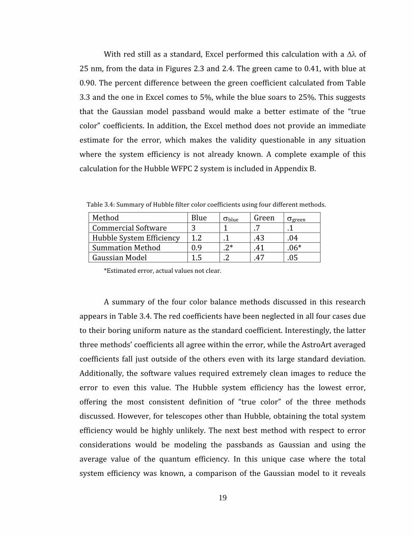
With red still as a standard, Excel performed this calculation with a of

25 nm, from the data in Figures 2.3 and 2.4. The green came to 0.41, with blue at

0.90. The percent difference between the green coefficient calculated from Table

3.3 and the one in Excel comes to 5%, while the blue soars to 25%. This suggests

that the Gaussian model passband would make a better estimate of the “true

color” coefficients. In addition, the Excel method does not provide an immediate

estimate for the error, which makes the validity questionable in any situation

where the system efficiency is not already known. A complete example of this

calculation for the Hubble WFPC 2 system is included in Appendix B.

Table 3.4: Summary of Hubble filter color coefficients using four different methods.

Method Blue blue Green green Commercial Software 3 1 .7 .1 Hubble System Efficiency 1.2 .1 .43 .04 Summation Method 0.9 .2* .41 .06* Gaussian Model 1.5 .2 .47 .05

*Estimated error, actual values not clear.

A summary of the four color balance methods discussed in this research

appears in Table 3.4. The red coefficients have been neglected in all four cases due

to their boring uniform nature as the standard coefficient. Interestingly, the latter

three methods’ coefficients all agree within the error, while the AstroArt averaged

coefficients fall just outside of the others even with its large standard deviation.

Additionally, the software values required extremely clean images to reduce the

error to even this value. The Hubble system efficiency has the lowest error,

offering the most consistent definition of “true color” of the three methods

discussed. However, for telescopes other than Hubble, obtaining the total system

efficiency would be highly unlikely. The next best method with respect to error

considerations would be modeling the passbands as Gaussian and using the

average value of the quantum efficiency. In this unique case where the total

system efficiency was known, a comparison of the Gaussian model to it reveals


that it agrees with the system efficiency with less than a 3% increase in the error.

This model could be applied to ground based telescopes anywhere in an attempt

to keep a consistent definition of “true color” in the astronomical image outputs.

21

Chapter 4

Ground Based Example

So far the color considerations in this project have been applied to space telescope

data which obviously did not include atmospheric considerations. By imposing a

restriction on shooting angles for ground based CCD images, the atmospheric

effects can be kept below 10%, rendering them negligible for the current

discussion. I will therefore ignore the atmosphere in the calculation of color

coefficients for ground based data with the understanding that the images will be

obtained reasonably close to the zenith.

As a ground based telescope example, the Orson Pratt Observatory on the

Brigham Young University campus has an SBIG ST-10XME detector, and standard

BVR Johnson filters. Using the filter passbands (Figure 2.1) and detector quantum

efficiency (Figure 2.2) obtained from the manufacturers, and setting red as the

standard 1.0 coefficient, blue becomes 1.8 ±.2 and green is 1.5 ± .2. (that

calculation was performed according to the method outlined in Appendix A). The

interesting advantage to following this procedure for a ground based setup is that

terrestrial objects can be photographed. A qualitative comparison of the final color

22 Chapter 4 Ground Based Example

balanced image can then be performed with the actual object, an impossibility

with astronomical objects.

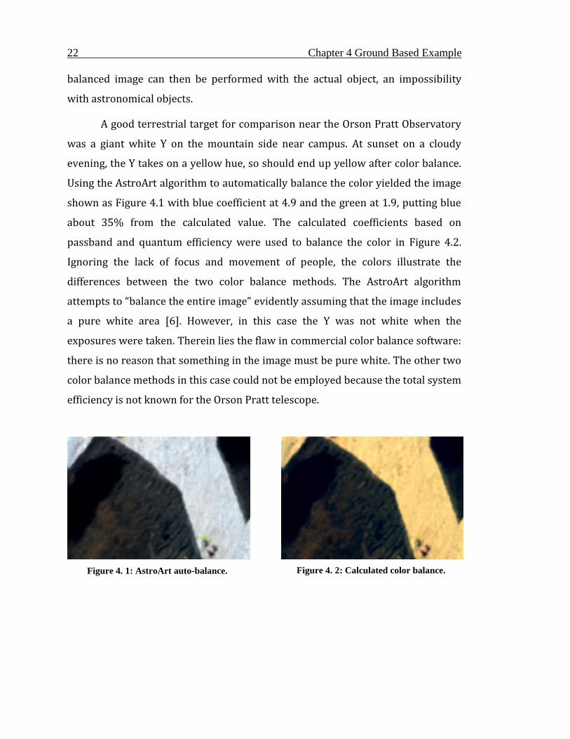
A good terrestrial target for comparison near the Orson Pratt Observatory

was a giant white Y on the mountain side near campus. At sunset on a cloudy

evening, the Y takes on a yellow hue, so should end up yellow after color balance.

Using the AstroArt algorithm to automatically balance the color yielded the image

shown as Figure 4.1 with blue coefficient at 4.9 and the green at 1.9, putting blue

about 35% from the calculated value. The calculated coefficients based on

passband and quantum efficiency were used to balance the color in Figure 4.2.

Ignoring the lack of focus and movement of people, the colors illustrate the

differences between the two color balance methods. The AstroArt algorithm

attempts to “balance the entire image” evidently assuming that the image includes

a pure white area [6]. However, in this case the Y was not white when the

exposures were taken. Therein lies the flaw in commercial color balance software:

there is no reason that something in the image must be pure white. The other two

color balance methods in this case could not be employed because the total system

efficiency is not known for the Orson Pratt telescope.

Figure 4. 1: AstroArt auto-balance.

Figure 4. 2: Calculated color balance.

23

Chapter 5

Conclusions

There are many possible methods for finding color balance coefficients for

astronomical images. While knowing the total system efficiency for each filter with

a given telescope provides the best ratio between colors, that information is not

available in enough detail to make that calculation useful for most telescopes and

detectors. Ignoring telescope geometry and atmospheric effects can still provide a

good estimation of relative light transmission between filters. This can lead to a

definition of “true color” by using these values to find dimensionless color balance

coefficients for each color exposure.

Modeling the filter passbands as Gaussian curves and finding the average

value of the quantum efficiency for each filter provides color coefficients with

error estimations comparable to the total system efficiency. Thus with less

required information comparable results can be obtained. This straight forward

calculation (see Appendix A) provides a consistent and useful definition of true

color for any ground based astronomical images. The resulting images can then be

used as qualitative composition or temperature maps with greater confidence in

the relevance of color assignments.

24 Chapter 5 Conclusions

An interesting extension of this research might attempt methods for

determining total system efficiency for ground based telescopes. This would

provide a method for comparison of images of the same objects from different

telescopes color balanced for each respective system, a good test for the

consistency of that definition of true color. The same process could be applied to

each color balance method, to find which method remained most consistent.

25

Bibliography

[1] S. Morel and E. Davoust, Software for producing trichromatic images in

astronomy, Experimental Astronomy, June 1995.

[2] S. K. Patra, M. Shekher, S. S. Solanki, R. Ramachandran, and R. Krishnan, A

technique for generating natural colour images from false color composite

images, International Journal of Remote Sensing, Vol. 27, No. 14, 20 July 2006,

2977-2989.

[3] P. Askey, Digital Photography Review, January 2004.

[4] B. Heyer et al., 2004, WFPC2 Instrument Handbook, Version 9.0 (Baltimore:

STScI).

[5] Space Telescope Science Institute. Retrieved July 22, 2008, from

ftp://ftp.stsci.edu/cdbs/comp/wfpc.

[6] F. Cavicchio, (private communication, July 2008).

[7] B. Berman, Astronomy, “The Real Twilight Zone,” Oct2007, Vol. 35 Issue 10,

p10-10, 1p, 1 color

[8] Santa Barbara Institute Group, Inc., November 2008. Retrieved November 4,

2008, from http://www.sbig.com/pdffiles/cat_filterwheels.pdf

[9] Santa Barbara Institute Group, Inc., November 2008. Retrieved November 4,

2008, from http://www.sbig.com/sbwhtmls/online.htm

26 Bibliography

[10] Space Telescope Science Institute. Retrieved July 2008, from

http://www.stsci.edu/hst/

[11] P. Bevington, Data Reduction and Error Analysis For the Physical Sciences, 1st

ed.; McGraw-Hill Inc.: New York, 1969; p 59.

[12] Laidler et al, 2005, "Synphot User's Guide," Version 5.0 (Baltimore, STScI).

27

Appendix A

Coefficient Calculation for Gaussian Model

The following calculation was performed for the Hubble WFPC2 detector with the

F450W, F606W, and F814W filters in Maple 11.

28 Chapter A Gaussian Model

29

(1)

(2)

(3)

(4)

(5)

(6)

30 Chapter A Gaussian Model

31

Appendix B

Summation Method Coefficient Calculation The estimate of total system throughput color balance method discussed in section 3.4 was performed in Excel for the Hubble WFPC2 detector and F450W, F606W, and F814W color filters. Table B.1 shows the values obtained, and Table B.2 shows the formula inputs.

32 Chapter B Summation Method

Table B.1: Coefficient calculation in Excel for Hubble WFPC2 filters.

Q()

B

T()

G

T() R T()

B

T()Q()d/

G

T()Q()d/

R

T()Q()d/

2000 0.01 0.00 0.00 0.00 0.0E+00 0.0E+00 0.0E+00 2000

2250 0.02 0.00 0.00 0.00 0.0E+00 0.0E+00 0.0E+00 2250

2500 0.02 0.00 0.00 0.00 0.0E+00 0.0E+00 0.0E+00 2500

2750 0.04 0.00 0.00 0.00 0.0E+00 0.0E+00 0.0E+00 2750

3000 0.04 0.00 0.00 0.00 0.0E+00 0.0E+00 0.0E+00 3000

3250 0.04 0.00 0.00 0.00 0.0E+00 0.0E+00 0.0E+00 3250

3500 0.05 0.01 0.00 0.00 3.2E-05 0.0E+00 0.0E+00 3500

3750 0.06 0.40 0.00 0.00 1.5E-03 0.0E+00 0.0E+00 3750

4000 0.06 0.80 0.00 0.00 3.0E-03 0.0E+00 0.0E+00 4000

4250 0.06 0.80 0.00 0.00 2.8E-03 0.0E+00 0.0E+00 4250

4500 0.06 0.90 0.00 0.00 3.1E-03 0.0E+00 0.0E+00 4500

4750 0.08 0.80 0.15 0.00 3.4E-03 6.3E-04 0.0E+00 4750

5000 0.10 0.90 0.80 0.00 4.3E-03 3.8E-03 0.0E+00 5000

5250 0.11 0.50 0.90 0.00 2.6E-03 4.7E-03 0.0E+00 5250

5500 0.14 0.02 0.90 0.00 1.3E-04 5.7E-03 0.0E+00 5500

5750 0.14 0.00 0.90 0.00 0.0E+00 5.5E-03 0.0E+00 5750

6000 0.15 0.00 0.90 0.00 0.0E+00 5.5E-03 0.0E+00 6000

6250 0.15 0.00 0.90 0.00 0.0E+00 5.3E-03 0.0E+00 6250

6500 0.15 0.00 0.90 0.00 0.0E+00 5.1E-03 0.0E+00 6500

6750 0.14 0.00 0.90 0.00 0.0E+00 4.7E-03 0.0E+00 6750

7000 0.12 0.00 0.50 0.40 0.0E+00 2.1E-03 1.7E-03 7000

7250 0.10 0.00 0.90 0.92 0.0E+00 3.1E-03 3.2E-03 7250

7500 0.10 0.00 0.01 0.89 0.0E+00 3.2E-05 2.8E-03 7500

7750 0.08 0.00 0.00 0.92 0.0E+00 0.0E+00 2.4E-03 7750

8000 0.07 0.00 0.00 0.90 0.0E+00 0.0E+00 2.0E-03 8000

8250 0.06 0.00 0.00 0.91 0.0E+00 0.0E+00 1.7E-03 8250

8500 0.06 0.00 0.00 0.92 0.0E+00 0.0E+00 1.6E-03 8500

8750 0.05 0.00 0.00 0.90 0.0E+00 0.0E+00 1.3E-03 8750

9000 0.04 0.00 0.00 0.85 0.0E+00 0.0E+00 9.4E-04 9000

9250 0.03 0.00 0.00 0.91 0.0E+00 0.0E+00 6.4E-04 9250

9500 0.02 0.00 0.00 0.92 0.0E+00 0.0E+00 4.8E-04 9500

9750 0.01 0.00 0.00 0.50 0.0E+00 0.0E+00 1.3E-04 9750

10000 0.01 0.00 0.00 0.02 0.0E+00 0.0E+00 4.5E-06 10000

10250 0.01 0.00 0.00 0.00 0.0E+00 0.0E+00 0.0E+00 10250

10500 0.00 0.00 0.00 0.00 0.0E+00 0.0E+00 0.0E+00 10500

Totals 0.02081 0.04623 0.01876

d 250 BLUE: GREEN: RED: d

0.90 0.41 1.00

33

Table B.2: Formulas for the summation method in Excel (values in Table B.1).

Q()

B

T()

G

T() R T() B T()Q()d/ G T()Q()d/ R T()Q()d/

2000 0.01 0 0 0 =B2*$B$38*C2/A2 =B2*$B$38*D2/A2 =B2*$B$38*E2/A2

=A2+$B$38 0.015 0 0 0 =B3*$B$38*C3/A3 =B3*$B$38*D3/A3 =B3*$B$38*E3/A3

=A3+$B$38 0.02 0 0 0 =B4*$B$38*C4/A4 =B4*$B$38*D4/A4 =B4*$B$38*E4/A4

=A4+$B$38 0.035 0 0 0 =B5*$B$38*C5/A5 =B5*$B$38*D5/A5 =B5*$B$38*E5/A5

=A5+$B$38 0.035 0 0 0 =B6*$B$38*C6/A6 =B6*$B$38*D6/A6 =B6*$B$38*E6/A6

=A6+$B$38 0.04 0 0 0 =B7*$B$38*C7/A7 =B7*$B$38*D7/A7 =B7*$B$38*E7/A7

=A7+$B$38 0.045 0.01 0 0 =B8*$B$38*C8/A8 =B8*$B$38*D8/A8 =B8*$B$38*E8/A8

=A8+$B$38 0.055 0.4 0 0 =B9*$B$38*C9/A9 =B9*$B$38*D9/A9 =B9*$B$38*E9/A9

=A9+$B$38 0.06 0.8 0 0 =B10*$B$38*C10/A10 =B10*$B$38*D10/A10 =B10*$B$38*E10/A10

=A10+$B$38 0.06 0.8 0 0 =B11*$B$38*C11/A11 =B11*$B$38*D11/A11 =B11*$B$38*E11/A11

=A11+$B$38 0.062 0.9 0 0 =B12*$B$38*C12/A12 =B12*$B$38*D12/A12 =B12*$B$38*E12/A12

=A12+$B$38 0.08 0.8 0.15 0 =B13*$B$38*C13/A13 =B13*$B$38*D13/A13 =B13*$B$38*E13/A13

=A13+$B$38 0.095 0.9 0.8 0 =B14*$B$38*C14/A14 =B14*$B$38*D14/A14 =B14*$B$38*E14/A14

=A14+$B$38 0.11 0.5 0.9 0 =B15*$B$38*C15/A15 =B15*$B$38*D15/A15 =B15*$B$38*E15/A15

=A15+$B$38 0.14 0.02 0.9 0 =B16*$B$38*C16/A16 =B16*$B$38*D16/A16 =B16*$B$38*E16/A16

=A16+$B$38 0.141 0 0.9 0 =B17*$B$38*C17/A17 =B17*$B$38*D17/A17 =B17*$B$38*E17/A17

=A17+$B$38 0.147 0 0.9 0 =B18*$B$38*C18/A18 =B18*$B$38*D18/A18 =B18*$B$38*E18/A18

=A18+$B$38 0.147 0 0.9 0 =B19*$B$38*C19/A19 =B19*$B$38*D19/A19 =B19*$B$38*E19/A19

=A19+$B$38 0.147 0 0.9 0 =B20*$B$38*C20/A20 =B20*$B$38*D20/A20 =B20*$B$38*E20/A20

=A20+$B$38 0.14 0 0.9 0 =B21*$B$38*C21/A21 =B21*$B$38*D21/A21 =B21*$B$38*E21/A21

=A21+$B$38 0.12 0 0.5 0.4 =B22*$B$38*C22/A22 =B22*$B$38*D22/A22 =B22*$B$38*E22/A22

=A22+$B$38 0.1 0 0.9 0.92 =B23*$B$38*C23/A23 =B23*$B$38*D23/A23 =B23*$B$38*E23/A23

=A23+$B$38 0.095 0 0.01 0.89 =B24*$B$38*C24/A24 =B24*$B$38*D24/A24 =B24*$B$38*E24/A24

=A24+$B$38 0.08 0 0 0.92 =B25*$B$38*C25/A25 =B25*$B$38*D25/A25 =B25*$B$38*E25/A25

=A25+$B$38 0.07 0 0 0.9 =B26*$B$38*C26/A26 =B26*$B$38*D26/A26 =B26*$B$38*E26/A26

=A26+$B$38 0.06 0 0 0.91 =B27*$B$38*C27/A27 =B27*$B$38*D27/A27 =B27*$B$38*E27/A27

=A27+$B$38 0.058 0 0 0.92 =B28*$B$38*C28/A28 =B28*$B$38*D28/A28 =B28*$B$38*E28/A28

=A28+$B$38 0.05 0 0 0.9 =B29*$B$38*C29/A29 =B29*$B$38*D29/A29 =B29*$B$38*E29/A29

=A29+$B$38 0.04 0 0 0.85 =B30*$B$38*C30/A30 =B30*$B$38*D30/A30 =B30*$B$38*E30/A30

=A30+$B$38 0.026 0 0 0.91 =B31*$B$38*C31/A31 =B31*$B$38*D31/A31 =B31*$B$38*E31/A31

=A31+$B$38 0.02 0 0 0.92 =B32*$B$38*C32/A32 =B32*$B$38*D32/A32 =B32*$B$38*E32/A32

=A32+$B$38 0.01 0 0 0.5 =B33*$B$38*C33/A33 =B33*$B$38*D33/A33 =B33*$B$38*E33/A33

=A33+$B$38 0.009 0 0 0.02 =B34*$B$38*C34/A34 =B34*$B$38*D34/A34 =B34*$B$38*E34/A34

=A34+$B$38 0.005 0 0 0 =B35*$B$38*C35/A35 =B35*$B$38*D35/A35 =B35*$B$38*E35/A35

=A35+$B$38 0.001 0 0 0 =B36*$B$38*C36/A36 =B36*$B$38*D36/A36 =B36*$B$38*E36/A36

Totals =SUM(F2:F36) =SUM(G2:G36) =SUM(H2:H36)

d 250 BLUE: GREEN: RED:

=H37/F37 =H37/G37 =H37/H37

Documents

TRUE COLOR BVR IMAGING by Heidi Dumais … · Heidi Dumais This thesis has been reviewed by the research committee, senior thesis coordinator, and department chair and has been found